Nonlinear Analysis 75 (2012) 3543–3551

Contents lists available at SciVerse ScienceDirect

Nonlinear Analysis

journal homepage: www.elsevier.com/locate/na

Hopf-type formula defines viscosity solution for Hamilton–Jacobiequations with t-dependence Hamiltonian

Nguyen Hoang ∗

Department of Mathematics, College of Education, Hue University, 3 LeLoi, Hue, Viet Nam

a r t i c l e i n f o

Article history:Received 9 November 2011Accepted 12 January 2012Communicated by S. Carl

In the memory of Prof. T.D. Van

Keywords:Hamilton–Jacobi equationHopf-type formulaViscosity solutionSemiconvexity

a b s t r a c t

Weprove that under some assumptions, the Hopf-type formula u(t, x) = maxq∈Rn ⟨x, q⟩−σ ∗(q) −

t0 H(τ , q)dτ defines a viscosity solution of the Cauchy problem for Hamil-

ton–Jacobi equation (H, σ ) where the initial condition σ is convex but the HamiltonianH = H(t, p) is not necessarily convex in p.

© 2012 Elsevier Ltd. All rights reserved.

1. Introduction

Consider the Cauchy problem for Hamilton–Jacobi equations of the form

∂u∂t

+ H(t, x,Dxu) = 0, (t, x) ∈ Ω = (0, T )× Rn, (1.1)

u(0, x) = σ(x), x ∈ Rn. (1.2)

The Hopf–Lax–Oleinik formula for solutions of the problem (1.1) and (1.2) is given by

u(t, x) = miny∈Rn

σ( y)+ tH∗

x − yt

, (1.3)

where the Hamiltonian H(t, x, p) = H(p) is convex and superlinear and σ is Lipschitz on Rn.If H(t, x, p) = H(p) is a continuous function and σ(x) is a convex Lipschitz function on Rn, then the Hopf formula is

u(t, x) = maxq∈Rn

⟨x, q⟩ − σ ∗(q)− tH(q). (1.4)

Here H∗ (resp., σ ∗) denotes the Fenchel conjugate of the convex function H (resp., σ ).Under suitable assumptions, these formulas give the viscosity solutions to the above Cauchy problem [1]. IfH = H(t, x, p)

is a convex function with respect to the last variable, then the general representation of the Hopf–Lax–Oleinik type formula(1.3) is established and studied thoroughly, using the calculus of variations; see [2] and references therein. If H(t, x, ·) is

This work is supported in part by NAFOSTED, Viet Nam.∗ Tel.: +84 54 3821700; fax: +84 54 3825902.

E-mail addresses: nguyenhoanghue@gmail.com, hoangboi2000@yahoo.com, nguyenhoang@hueuni.edu.vn.

0362-546X/$ – see front matter© 2012 Elsevier Ltd. All rights reserved.doi:10.1016/j.na.2012.01.013

3544 N. Hoang / Nonlinear Analysis 75 (2012) 3543–3551

nonconvex, the Hamiltonians H = H(p) can be expanded to the forms H = H(u, p) or H = H(t, p) to get generalizedsolutions such as Lipschitz or viscosity solutions. Nevertheless, many questions remain open for the case of nonconvexHamiltonians.

Naturally, it is expected that the formula

u(t, x) = maxq∈Rn

⟨x, q⟩ − σ ∗(q)−

t

0H(τ , q)dτ

(1.5)

defines a viscosity solution as a generalization of formula (1.4) under the assumptions that H = H(t, p) is continuous andσ is convex.

Unfortunately, as in [3], Lions and Rochet showed that it is not a viscosity solution in general, although it is a Lipschitzsolution under some compatible conditions between H(t, p) and σ(x); see [4]. The weakness of the notion of Lipschitzsolution is that the uniqueness of the solution is not guaranteed.

Under different hypotheses, some results on the representation of the viscosity solution of the problem are established.For example, in [5] Silin constructed the notion of conjugate integral to deal the context whereH(t, p) satisfies the followingcondition

|H(t1, p)− H(t2, p)| ≤ ω(|t1 − t2|),

for all t1, t2 ∈ [0, T ] and p ∈ Rn. Here ω(·) is a modulus.This paper is devoted to proving that formula (1.5) defines a viscosity solution of the problem (1.1)–(1.2) for a class of

Hamiltonians H = H(t, p). In Section 2, we first recall some definitions and properties of semiconvex functions as well assub- and superdifferential of a function. Then we prove that u(t, x) defined by (1.5) is a semiconvex function. In Section 3,we check a ‘‘consecutiveness property’’ of H = H(t, p) and σ(x): it is the ‘‘semigroup property’’ in case H = H(p) and σ(x);see [3]. Furthermore, based on a property of the subdifferential of semiconvex functions, analogous to convex functions, weadapt the proof of Lions and Rochet in [3] to verify that u(t, x) is actually a viscosity solution. Next, we use the relationshipbetween subdifferential D−u(t, x) and the set of all reachable gradients D∗u(t, x) to prove that u(t, x) is also a viscositysolution in case Hamiltonian H(t, p) is concave in p.

The results obtained here are new for a large class of nonconvex Hamiltonians H(t, p). However, they may not exhaustall possible cases for u(t, x) to be a viscosity solution.

We use the following notations. Let T be a positive number,Ω = (0, T ) × Rn; | . | and ⟨., .⟩ be the Euclidean norm and

the scalar product in Rn, respectively, and let B′(x0, r) be the closed ball centered at x0 with radius r.

2. Preliminaries and semiconvexity of the Hopf-type formula

2.1. Assumptions

We now consider the Cauchy problem for the Hamilton–Jacobi equation:

∂u∂t

+ H(t,Dxu) = 0, (t, x) ∈ Ω = (0, T )× Rn, (2.1)

u(0, x) = σ(x), x ∈ Rn, (2.2)

where the Hamiltonian H(t, p) is of class C([0, T ] × Rn) and σ(x) ∈ C(Rn) is a convex function.Let σ ∗ be the Fenchel conjugate of σ . We denote by

D = dom σ ∗= y ∈ Rn

| σ ∗( y) < +∞

the effective domain of the convex function σ ∗.Throughout the paper, we use the following assumptions:

(A1): For every (t0, x0) ∈ [0, T )× Rn, there exist positive constants r and N such that

⟨x, p⟩ − σ ∗(p)−

t

0H(τ , p)dτ < max

|q|≤N

⟨x, q⟩ − σ ∗(q)−

t

0H(τ , q)dτ

,

whenever (t, x) ∈ [0, T )× Rn, |t − t0| + |x − x0| < r and |p| > N.(A2): H(t, p) is admitted as one of two following forms:(a) H(t, ·) is a convex function for all t ∈ (0, T ).(b) H(t, p) = g(t)h(p)+ k(t) for some functions g, h, kwhere g(t) does not change its sign for all t ∈ (0, T ).

Remark 2.1. (a) The assumption (A1) can be considered as a compatible condition for the Hamiltonian H(t, p) and initialdata σ(x), primarily used in [6].

(b) If σ(x) is Lipschitz continuous on Rn, then D = domσ ∗ is bounded. Consequently, the condition (A1) is automaticallysatisfied.

(c) If H(t, p) = H(p), then the condition (A2), (b) is obviously satisfied.

N. Hoang / Nonlinear Analysis 75 (2012) 3543–3551 3545

Denote

u(t, x) = maxq∈Rn

⟨x, q⟩ − σ ∗(q)−

t

0H(τ , q)dτ

. (2.3)

For each (t, x) ∈ Ω , let ℓ(t, x) be the set of all p ∈ Rn at which the maximum of the function q → ⟨x, q⟩ − σ ∗(q) − t0 H(τ , q)dτ is attained. In virtue of (A1), ℓ(t, x) = ∅.

Definition 2.2. The function u(t, x) defined by (2.3) is called the Hopf-type formula for the Cauchy problem (2.1)–(2.2).

Now we assume condition (A1). Then u(t, x) is a locally Lipschitz continuous function onΩ that satisfies Eq. (2.1) at thepoints that u(t, x) is differentiable and u(0, x) = σ(x), x ∈ Rn, i.e., it is a Lipschitz solution of the problem; see [4,7].

2.2. Sub- and superdifferential of a function.

Let v : Ω → R be a function and let y = (t, x) ∈ Ω .Wedenote byD+v( y) (resp.,D−v( y)) the set of allp = (p, q) ∈ Rn+1

such that:

D+v( y) =

p ∈ Rn+1

| lim suph→0

v( y + h)− v( y)− ⟨p, h⟩|h|

≤ 0

(resp.

D−v( y) =

p ∈ Rn+1

| lim infh→0

v( y + h)− v( y)− ⟨p, h⟩|h|

≥ 0.)

We call D+v( y) (resp., D−v( y)) superdifferential (resp. subdifferential) of the function v( y) at y = (t, x) ∈ Ω.

We suppose that v( y) is a locally Lipschitz function onΩ . Then the upper and lower Dini directional derivatives of v( y)at y in the direction e ∈ Rn+1, denoted by ∂+

e v( y) and ∂−e v( y), are defined as follows:

∂+

e v( y) = lim sups↓0

v( y + se)− v( y)s

and

∂−

e v( y) = lim infs↓0

v( y + se)− v( y)s

.

We recall a relationship between D+v( y) and ∂+e v( y) (resp. D

−v( y) and ∂−e v( y)) as follows:

D+v( y) = p ∈ Rn+1| ∂+

e v( y) ≤ ⟨p, e⟩, ∀e ∈ Rn+1

(resp.

D−v( y) = p ∈ Rn+1| ∂−

e v( y) ≥ ⟨p, e⟩, ∀e ∈ Rn+1.)

2.3. Semiconvexity of the Hopf-type formula

Definition 2.3. A function v : Ω → R is called a semiconvex functionwith linear modulus if there is a constant C > 0 suchthat

v(λy1 + (1 − λ)y2)− λv( y1)− (1 − λ)v( y2) ≤ λ(1 − λ)C2

|y1 − y2|2

for any pair y1 = (t1, x1), y2 = (t2, x2) inΩ and for any λ ∈ [0, 1].

Note that, the theory of semiconcave functions was developed in last decades of previous century for more generalmodulus, and recently it is presented systematically in [2].

The function v is semiconvex if and only if −v is semiconcave. In this paper we therefore use some properties ofsemiconvex functions transferred from the ones of semiconcave functions.

An important property of the function u(t, x) defined by the Hopf-type formula is given by the following theorem.

Theorem 2.4. Suppose that H(t, p) ∈ C1([0, T ] × Rn) and σ(x) is convex and Lipschitz on Rn. Then the Hopf-type formulau(t, x) defined by (2.3) is a semiconvex function onΩ.

3546 N. Hoang / Nonlinear Analysis 75 (2012) 3543–3551

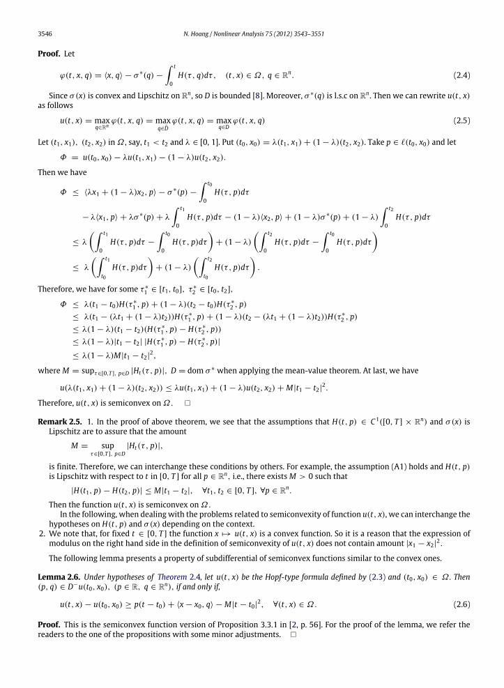
Proof. Let

ϕ(t, x, q) = ⟨x, q⟩ − σ ∗(q)−

t

0H(τ , q)dτ , (t, x) ∈ Ω, q ∈ Rn. (2.4)

Since σ(x) is convex and Lipschitz on Rn, so D is bounded [8]. Moreover, σ ∗(q) is l.s.c on Rn. Then we can rewrite u(t, x)as follows

u(t, x) = maxq∈Rn

ϕ(t, x, q) = maxq∈D

ϕ(t, x, q) = maxq∈D

ϕ(t, x, q) (2.5)

Let (t1, x1), (t2, x2) inΩ , say, t1 < t2 and λ ∈ [0, 1]. Put (t0, x0) = λ(t1, x1)+ (1 − λ)(t2, x2). Take p ∈ ℓ(t0, x0) and let

Φ = u(t0, x0)− λu(t1, x1)− (1 − λ)u(t2, x2).

Then we have

Φ ≤ ⟨λx1 + (1 − λ)x2, p⟩ − σ ∗(p)−

t0

0H(τ , p)dτ

− λ⟨x1, p⟩ + λσ ∗(p)+ λ

t1

0H(τ , p)dτ − (1 − λ)⟨x2, p⟩ + (1 − λ)σ ∗(p)+ (1 − λ)

t2

0H(τ , p)dτ

≤ λ

t1

0H(τ , p)dτ −

t0

0H(τ , p)dτ

+ (1 − λ)

t2

0H(τ , p)dτ −

t0

0H(τ , p)dτ

≤ λ

t1

t0H(τ , p)dτ

+ (1 − λ)

t2

t0H(τ , p)dτ

.

Therefore, we have for some τ ∗

1 ∈ [t1, t0], τ ∗

2 ∈ [t0, t2],

Φ ≤ λ(t1 − t0)H(τ ∗

1 , p)+ (1 − λ)(t2 − t0)H(τ ∗

2 , p)≤ λ(t1 − (λt1 + (1 − λ)t2))H(τ ∗

1 , p)+ (1 − λ)(t2 − (λt1 + (1 − λ)t2))H(τ ∗

2 , p)≤ λ(1 − λ)(t1 − t2)(H(τ ∗

1 , p)− H(τ ∗

2 , p))≤ λ(1 − λ)|t1 − t2| |H(τ ∗

1 , p)− H(τ ∗

2 , p)|

≤ λ(1 − λ)M|t1 − t2|2,

where M = supτ∈[0,T ], p∈D |Ht(τ , p)|, D = dom σ ∗ when applying the mean-value theorem. At last, we have

u(λ(t1, x1)+ (1 − λ)(t2, x2)) ≤ λu(t1, x1)+ (1 − λ)u(t2, x2)+ M|t1 − t2|2.

Therefore, u(t, x) is semiconvex onΩ.

Remark 2.5. 1. In the proof of above theorem, we see that the assumptions that H(t, p) ∈ C1([0, T ] × Rn) and σ(x) isLipschitz are to assure that the amount

M = supτ∈[0,T ], p∈D

|Ht(τ , p)|,

is finite. Therefore, we can interchange these conditions by others. For example, the assumption (A1) holds and H(t, p)is Lipschitz with respect to t in [0, T ] for all p ∈ Rn, i.e., there existsM > 0 such that

|H(t1, p)− H(t2, p)| ≤ M|t1 − t2|, ∀t1, t2 ∈ [0, T ], ∀p ∈ Rn.

Then the function u(t, x) is semiconvex onΩ.In the following, when dealing with the problems related to semiconvexity of function u(t, x), we can interchange the

hypotheses on H(t, p) and σ(x) depending on the context.2. We note that, for fixed t ∈ [0, T ] the function x → u(t, x) is a convex function. So it is a reason that the expression of

modulus on the right hand side in the definition of semiconvexity of u(t, x) does not contain amount |x1 − x2|2.

The following lemma presents a property of subdifferential of semiconvex functions similar to the convex ones.

Lemma 2.6. Under hypotheses of Theorem 2.4, let u(t, x) be the Hopf-type formula defined by (2.3) and (t0, x0) ∈ Ω . Then(p, q) ∈ D−u(t0, x0), (p ∈ R, q ∈ Rn), if and only if,

u(t, x)− u(t0, x0) ≥ p(t − t0)+ ⟨x − x0, q⟩ − M|t − t0|2, ∀(t, x) ∈ Ω. (2.6)

Proof. This is the semiconvex function version of Proposition 3.3.1 in [2, p. 56]. For the proof of the lemma, we refer thereaders to the one of the propositions with some minor adjustments.

N. Hoang / Nonlinear Analysis 75 (2012) 3543–3551 3547

3. A viscosity solution

3.1. ‘‘Consecutiveness property’’

For a given function v(x) on Rn, let the Fenchel conjugate of v be

v∗(x) = supy∈Rn

⟨x, y⟩ − v( y)

and v∗∗= (v∗)∗ the second Fenchel conjugate of v(x). We know that v∗∗ is the greatest convex function bounded above by

v. If v : Rn→ R is convex, then v = v∗∗.

The following proposition is necessary to prove the next theorem.

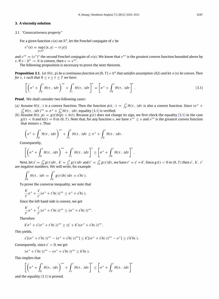
Proposition 3.1. Let H(t, p) be a continuous function on [0, T ]×Rn that satisfies assumption (A2) and let σ(x) be convex. Thenfor s, t such that 0 ≤ s ≤ t ≤ T we have:

σ ∗+

s

0H(τ , ·)dτ

∗∗

+

t

sH(τ , ·)dτ

∗

=

σ ∗

+

t

0H(τ , ·)dτ

∗

. (3.1)

Proof. We shall consider two following cases:

(a) Assume H(t, ·) is a convex function. Then the function φ(t, ·) = t0 H(τ , ·)dτ is also a convex function. Since (σ ∗

+ s0 H(τ , ·)dτ)∗∗

= σ ∗+ s0 H(τ , ·)dτ , equality (3.1) is verified.

(b) Assume H(t, p) = g(t)h(p) + k(t). Because g(t) does not change its sign, we first check the equality (3.1) in the caseg(t) < 0 and k(t) = 0 in (0, T ). Note that, for any function v, we have v∗∗

≤ v and v∗∗ is the greatest convex functionthat minors v. Thus

σ ∗+

s

0H(τ , ·)dτ

∗∗

+

t

sH(τ , ·)dτ ≤ σ ∗

+

t

0H(τ , ·)dτ .

Consequently,σ ∗

+

s

0H(τ , ·)dτ

∗∗

+

t

sH(τ , ·)dτ

∗

≥

σ ∗

+

t

0H(τ , ·)dτ

∗

.

Next, let s′ = s0 g(τ )dτ , k′

= ts g(τ )dτ and t ′ =

t0 g(τ )dτ , we have t ′ = s′ + k′. Since g(t) < 0 in (0, T ) then s′, k′, t ′

are negative numbers. We will write, for example s

0H(τ , ·)dτ =

s

0g(τ )h(·)dτ = s′h(·).

To prove the converse inequality, we note that

k′

t ′σ ∗

+s′

t ′(σ ∗

+ t ′h(·))∗∗≤ σ ∗

+ s′h(·).

Since the left hand side is convex, we get

k′

t ′σ ∗

+s′

t ′(σ ∗

+ t ′h(·))∗∗≤ (σ ∗

+ s′h(·))∗∗.

Therefore

k′σ ∗+ s′(σ ∗

+ t ′h(·))∗∗≥ (s′ + k′)(σ ∗

+ s′h(·))∗∗.

This yields,

s′[(σ ∗+ t ′h(·))∗∗

− (σ ∗+ s′h(·))∗∗

] ≥ k′[(σ ∗

+ s′h(·))∗∗− σ ∗

] ≥ s′k′h(·).

Consequently, since s′ < 0, we get

(σ ∗+ t ′h(·))∗∗

− (σ ∗+ s′h(·))∗∗

≤ k′h(·).

This implies thatσ ∗

+

s

0H(τ , ·)dτ

∗∗

+

t

sH(τ , ·)dτ

∗

≤

σ ∗

+

t

0H(τ , ·)dτ

∗

and the equality (3.1) is proved.

3548 N. Hoang / Nonlinear Analysis 75 (2012) 3543–3551

Similarly, we easily check the equality in the case g(t) > 0 in (0, T ). Finally, note that, for arbitrary function v andconstant α, by definition we have

(v + α)∗ = v∗− α.

Then

(v + α)∗∗= (v∗

− α)∗ = v∗∗+ α.

Hence,σ ∗

+

s

0H(τ , ·)dτ + α1

∗∗

+

t

sH(τ , ·)dτ + α2

∗

=

σ ∗

+

t

0H(τ , ·)dτ + α

∗

,

where α1 = s0 k(τ )dτ , α2 =

ts k(τ )dτ , α =

t0 k(τ )dτ and α = α1 + α2.

The proof is then complete.

Remark 3.2. Denote

(Cts )(σ ) =

σ ∗

+

t

sH(τ , ·)dτ

∗

, 0 ≤ s ≤ t ≤ T .

Then the equality (3.1) can be rewritten as

(Cts )(C

s0(σ )) = (Ct

0)(σ ).

In other words,

Cts Cs

0 = Ct0.

We call this equality the ‘‘consecutiveness property’’ or ‘‘C-property’’ of H and σ . If H is independent of t , i.e., H = H(p),then the above property turns out to be ‘‘semigroup property’’, see [9,3]

S(t) S(s) = S(t + s),

where S(t)(σ ) = (σ ∗+ tH)∗.

3.2. A viscosity solution defined by the Hopf-type formula

Theorem 3.3. Assume (A1), (A2). Moreover, let H(t, p) ∈ C1([0, T ]×Rn). Then the Hopf-type formula u(t, x) defined by (2.3) isa viscosity solution of the Cauchy problem (2.1)–(2.2)

Proof. We divide the proof into two steps as follows.Step 1. We temporarily use an additional assumption that, σ(x) is Lipschitz continuous on Rn.

Wewill prove that u(t, x) is a viscosity supersolution. To this end, by definition, let (t0, x0) ∈ Ω and (p, q) ∈ D−u(t0, x0),we have to verify the inequality:

p + H(t0, q) ≥ 0.

By Theorem 2.4, u(t, x) is a semiconvex function onΩ. Using a property of subdifferential of u(t, x) given by Lemma 2.6,then for all (t, x) ∈ Ω,we have

u(t, x) ≥ u(t0, x0)+ ⟨q, x − x0⟩ + p(t − t0)− M|t − t0|2.

Put

ψ(t, x) = u(t0, x0)+ ⟨q, x − x0⟩ + p(t − t0)− M|t − t0|2.

Then we have u(t, x) ≥ ψ(t, x), ∀x ∈ Rn, t ∈ [0, T ].

Using the equality (3.1), we see that

u(t0, x0) =

σ ∗

+

t0

0H(τ , ·)dτ

∗

(x0)

=

σ ∗

+

t0−s

0H(τ , ·)dτ

∗∗

+

t0

t0−sH(τ , ·)dτ

∗

(x0). (3.2)

N. Hoang / Nonlinear Analysis 75 (2012) 3543–3551 3549

Note that, if v1 ≤ v2 then v∗∗

1 ≤ v∗∗

2 , and applying equality (3.2) we get

u(t0, x0) =

u∗(t0 − s, ·)+

t0

t0−sH(τ , ·)dτ

∗

(x0)

≥

ψ∗(t0 − s, ·)+

t0

t0−sH(τ , ·)dτ

∗

(x0). (3.3)

We have

ψ∗(t0 − s, z) = supx∈Rn

⟨z, x⟩ − u(t0, x0)− ⟨q, x − x0⟩ + ps + Ms2

= supx∈Rn

⟨z − q, x⟩ − u(t0, x0)+ ⟨q, x0⟩ + ps + Ms2

Thereforeψ∗(t0 − s, z) = −u(t0, x0)+ ⟨q, x0⟩ + ps + Ms2, if z = q+∞, if z = q.

Inequality (3.3) gives us:

u(t0, x0) ≥ supz∈Rn

⟨x0, z⟩ − ψ∗(t0 − s, z)−

t0

t0−sH(τ , z)dτ

≥ ⟨x0, q⟩ + u(t0, x0)− ⟨x0, q⟩ − ps − Ms2 −

t0

t0−sH(τ , q)dτ .

As a result, t0

t0−sH(τ , q)dτ + ps + Ms2 ≥ 0,

or,

sH(τ ∗, q)+ ps + Ms2 ≥ 0,

where τ ∗∈ [t0 − s, t0]. Dividing both sides by s then letting s → 0 we have

p + H(t0, q) ≥ 0.

Next, we check that u(t, x) is a viscosity subsolution. Since u(t, x) is semiconvex, then D−u(t, x) = ∅ for all (t, x) ∈ Ω.Let (t0, x0) ∈ Ω and (p, q) ∈ D+u(t0, x0). If D+u(t0, x0) = ∅, then the inequality p + H(t0, q) ≤ 0 is automatically

satisfied. If D+u(t0, x0) = ∅ then u(t, x) is differentiable and satisfies Eq. (2.1) at (t0, x0); see [4]. Therefore, ℓ(t0, x0) = qis a singleton and we have p = ut(t0, x0) = −H(t0, q), ux(t0, x0) = q. Thus, p + H(t0, q) = 0.

By definition, we conclude that u(t, x) is a viscosity solution of the problem.Step 2. We prove that u(t, x) is a viscosity solution in general case that σ(x) need not be Lipschitz continuous on Rn.

For everym ∈ N, let

vm(p) =

σ ∗(p), if |p| ≤ m+∞, if |p| > m.

Then vm is a lower semicontinuous convex function on Rn with dom vm ⊂ B′(0,m).Let

σm(x) = v∗

m(x) = supp∈Rn

⟨x, p⟩ − vm(p) = sup|p|≤m

⟨x, p⟩ − vm(p).

Then

σ ∗

m(x) = v∗∗

m (x) = vm(x).

Note that, σm(x) is a convex, Lipschitz continuous function on Rn.Applying the result of Step 1, we see that the function

um(t, x) = maxq∈Rn

⟨x, q⟩ − σ ∗

m(q)−

t

0H(τ , q)dτ

(3.4)

is a viscosity solution of the problem (H, σm).

3550 N. Hoang / Nonlinear Analysis 75 (2012) 3543–3551

By definition, the sequence (σm(x))m (resp. (um(t, x))m) is increasing and converges to the continuous function σ(x) onRn (resp. u(t, x) onΩ). Applying Dini’s theorem, we see that (σm(x))m (resp. (um(t, x))m) is locally uniformly convergent toσ(x) (resp. u(t, x)) on compact sets of Rn (resp.Ω).

Using the stability property of the viscosity solution [9], we conclude that, u(t, x) is indeed a viscosity solution of theproblem and the theorem is then proved.

We have seen that ‘‘C-property’’ is used as a sufficient condition to prove that the Hopf-type formula (2.3) is a viscositysolution. Therefore any class of Hamiltonians H(t, p) satisfying ‘‘C-property’’ will be the case.

Remark 3.4. The condition that g(t) does not change its sign on (0, T ) seems a technical requirement to prove the equality(3.1). Nevertheless, if this condition is violated, then the function u(t, x) defined by the Hopf-type formula is not a viscositysolution as in the following example.

Example. Consider the following Cauchy problem:ut + (2t − 1)u2

x = 0, (t, x) ∈ (0, 2)× R,u(0, x) = |x|, x ∈ R.

Then the Hopf-type formula of the problem is

u(t, x) = maxp∈[−1,1]

xp − (t2 − t)p2.

Let (t0, x0) = (1, 0). Then u(1, 0) = 0 and ℓ(1, 0) = [−1, 1]. Now we define the set D−u(1, 0). Using the relationbetween D−u(t, x) and ∂eu(t, x)where e = (α1, α2) and formula

∂eu(t, x) = maxq∈ℓ(t,x)

−α1H(t, q)+ α2q

see [4], we get that

∂eu(1, 0) = maxz∈[−1,1]

−α1z2 + α2z

and, therefore

(p, q) ∈ D−u(1, 0) if and only if, ∂eu(1, 0) ≥ α1p + α2q, ∀e = (α1, α2) ∈ R2.

It is easy to see that (−1, 0) ∈ D−u(1, 0) since

∂eu(1, 0) = maxz∈[−1,1]

−α1z2 + α2z ≥ −α1 + α2.0 = −α1, ∀e = (α1, α2) ∈ R2.

On the other hand, at (1, 0)we have p+H(1, q) = −1+1.0 = −1 < 0. Therefore u(t, x) is not a viscosity supersolution.The reason is that, the Hamiltonian H(t, p) = (2t − 1)p2, where g(t) = 2t − 1 changes its sign on [0, 2].

3.3. A viscosity solution for the concave Hamiltonian

Now we prove the Hopf-type formula is a viscosity solution under a different assumption for the Hamiltonian.Let u(t, x) be the Hopf-type formula (2.3). We use some notions and results from [2] as follows.Denote by D∗u(t, x) ⊂ R × Rn the set of all reachable gradients of u(t, x) at (t, x), that is,(p, q) ∈ D∗u(t, x) if and only if there exists a sequence (tk, xk)k ⊂ Ω \ (t, x) such that u(t, x) is differentiable at (tk, xk)

and,

(tk, xk) → (t, x), (ut(tk, xk), ux(tk, xk)) → (p, q) as k → ∞.

Since u(t, x) is locally Lipschitz, then D∗u(t, x) = ∅ and it is a compact set. Moreover, if u(t, x) is semiconvex, then wehave: D−u(t, x) = coD∗u(t, x), the convex hull of D∗u(t, x).

The difference between the proof of the following theorem and the one of Theorem 3.3 is that we interchange the ‘‘C-property’’ by a relation between D−u(t, x) and D∗u(t, x).

Theorem 3.5. Assume (A1). Let H(t, p) ∈ C1([0, T ] × Rn) be a concave function in variable p for all t ∈ (0, T ). Then theHopf-type formula (2.3) is a viscosity solution of the problem (2.1)–(2.2).

Proof. First, we prove the theoremwith an extra assumption that σ(x) is Lipschitz onRn. Then theHopf-type formula u(t, x)is a semiconvex function.

We check that u(t, x) is a viscosity supersolution. Let (p, q) ∈ D∗u(t0, x0) and sequence (tk, xk)k ⊂ Ω \ (t0, x0) suchthat u(t, x) is differentiable at (tk, xk) and (tk, xk) → (t0, x0), (ut(tk, xk), ux(tk, xk)) → (p, q) as k → ∞. Since

ut(tk, xk)+ H(tk, ux(tk, xk)) = 0

for all k, then passing k → ∞ we have p + H(t0, q) = 0.

N. Hoang / Nonlinear Analysis 75 (2012) 3543–3551 3551

Now, take (p, q) ∈ D−u(t0, x0). Then there exist αi ≥ 0,k

i=1 αi = 1 and (pi, qi) ∈ D∗u(t, x), i = 1, . . . , k such that

(p, q) =

ki=1

αi(pi, qi) =

k

i=1

αipi,k

i=1

αiqi

.

Then

p + H(t0, q) =

ki=1

αipi + H

t0,

ki=1

αiqi

≥

ki=1

αi(pi + H(t0, qi)) = 0.

Therefore, u(t, x) is a viscosity supersolution. To prove u(t, x) is a subsolution of the problemwe argue as in the proof ofTheorem 3.3.

Finally, we also use the limit process as in Step 2 of the proof of Theorem 3.3 to deal the case σ(x) is not Lipschitz. Thetheorem is then proved.

Remark 3.6. We will refer to some results on the uniqueness of the viscosity solution of the Cauchy problem (2.1)–(2.2),for example [9,10], . . . . Then the ‘‘C-property’’ (3.1) for the concave Hamiltonian H(t, p) and convex initial data σ(x) can beobtained while it seems that a direct proof will be more difficult.

Nowwe can use the equality D−u(t, x) = coD∗u(t, x) of the semiconvex function to verify a differentiability property ofthe viscosity solution u(t, x) as follows.

Proposition 3.7. Let H(t, p) ∈ C1([0, T ] × Rn) be a strictly convex function in variable p and σ(x) is a convex and Lipschitzfunction on Rn. Then the viscosity solution u(t, x) of the problem (2.1)–(2.2) is of class C1(Ω).

Proof. By assumption, the viscosity solution u(t, x) of the problem defined by the Hopf-type formula is a semiconvexfunction. To prove u(t, x) is of class C1(Ω), we check that, for any (t, x) ∈ Ω , the set D−u(t, x) is a singleton; see [2].Indeed, if it is converse, there exists (t0, x0) such that D−u(t0, x0) contains more than one element, so does D∗u(t0, x0) sinceD−u(t0, x0) = coD∗u(t0, x0). Let (pi, qi) ∈ D∗u(t0, x0), i = 1, 2, then we have

p1 + p22

+ Ht0,

q1 + q22

<

12[p1 + H(t0, q1)+ p2 + H(t0, q2)] = 0

because pi + H(t0, qi) = 0, i = 1, 2 as in the proof of Theorem 3.5. This is a contradiction sincep1 + p2

2,q1 + q2

2

∈ D−u(t0, x0)

and u(t, x) is a viscosity supersolution.

Remark 3.8. 1. This regularity result can also be deduced from the investigation of maximum of function ϕ(t, x, p) =

⟨x, p⟩ − σ ∗(p) − t0 H(τ , p)dτ . Actually, in this situation, the function p → ϕ(t, x, p) is strictly concave, therefore it

attains maximum at unique point q ∈ Rn. Alternatively, we also obtain the same result if p → H(t, p) is assumed convexand σ(x) is strictly convex. Consequently, ℓ(t, x) is a singleton for all (t, x) ∈ Ω , and u(t, x) ∈ C1(Ω) [4,7].

2. We present in another paper [11] more details of regularity of the viscosity solution of the Cauchy problem (2.1)–(2.2)defined by the Hopf-type formula regarding characteristics.

References

[1] M. Bardi, L.C. Evans, OnHopf’s formulas for solutions of Hamilton–Jacobi equations, Nonlinear Anal. Theory,Meth. & Appl., N. 11 (8) (1984) 1373–1831.[2] P. Cannarsa, C. Sinestrari, Semiconcave Functions, Hamilton–Jacobi Equations and Optimal Control, Birkhauser, Boston, 2004.[3] J.P. Lions, Rochet, Hopf formula and multitime Hamilton–Jacobi equation, Proc. AMS. 96 (1) (1986).[4] Tran Duc Van, Nguyen Hoang, Tsuji M., On Hopf’s formula for Lipschitz solutions of the Cauchy problem for Hamilton–Jacobi equations, Nonlinear

Anal. 29 (10) (1997) 1145–1159.[5] D.B. Silin, Generalizing Hopf and Oleinik formulae via conjugate integral, Mh. Math. 124 (1997) 343–364.[6] Tran Duc Van, Nguyen Hoang, Nguyen Duy Thai Son, On the explicit representation of global solutions of the Cauchy problem for Hamilton–Jacobi

equations, Acta Math. Viet. 19 (2) (1994) 111–120.[7] Tran Duc Van, Mikio Tsuji, Nguyen Duy Thai Son, The Characteristic Method and its Generalizations for First Order Nonlinear PDEs, Chapman &

Hall/CRC, 2000.[8] T. Rockafellar, Convex Analysis, Princeton Univ. Press, 1970.[9] M.G. Crandall, L.C. Evans, P.L. Lions, Some properties of viscosity solutions of Hamilton–Jacobi equations, Trans. Amer. Math. Soc. 282 (1984) 487–502.

[10] H. Ishii, Uniqueness of unbounded viscosity solution of Hamilton–Jacobi equations, Indiana Univ. Math. J. 33 (1984) 721–748.[11] Nguyen Hoang, Regularity of viscosity solutions defined by Hopf-type formula for Hamilton–Jacobi equations (submitted for publication).