Homology of Group Von Neumann Algebras

Wade Mattox

Dissertation submitted to the Faculty of the

Virginia Polytechnic Institute and State University

in partial fulfillment of the requirements for the degree of

Doctor of Philosophy

in

Mathematics

Peter Linnell, Chair

Bill Floyd

Peter Haskell

Jim Thomson

July 17, 2012

Blacksburg, Virginia

Keywords: Homology, Von Neumann Algebra, Group Theory

Copyright 2012, Wade Mattox

Homology of Group Von Neumann Algebras

Wade Mattox

(ABSTRACT)

In this paper the following conjecture is studied: the group von Neumann algebra N (G) is a

flat CG-module if and only if the group G is locally virtually cyclic. This paper proves that

if G is locally virtually cyclic, then N (G) is flat as a CG-module. The converse is proved

for the class of all elementary amenable groups without infinite locally finite subgroups.

Foundational cases for which the conjecture is shown to be true are the groups G = Z,

G = Z ⊕ Z, G = Z ∗ Z, Baumslag-Solitar groups, and some infinitely-presented variations

of Baumslag-Solitar groups. Modules other than N (G), such as `p-spaces and group C∗-

algebras, are considered as well. The primary tool that is used to achieve many of these

results is group homology.

Contents

1 Preliminary Material 1

1.1 Introduction and Main Results . . . . . . . . . . . . . . . . . . . . . . . . . . 1

1.2 Group Theory Terminology . . . . . . . . . . . . . . . . . . . . . . . . . . . 3

1.3 Motivation for Group Von Neumann Algebras . . . . . . . . . . . . . . . . . 4

1.4 Group Von Neumann Algebras . . . . . . . . . . . . . . . . . . . . . . . . . . 7

1.5 Von Neumann Dimension . . . . . . . . . . . . . . . . . . . . . . . . . . . . 9

1.6 Algebras of Affiliated Operators . . . . . . . . . . . . . . . . . . . . . . . . . 11

1.7 Left Modules vs. Right Modules . . . . . . . . . . . . . . . . . . . . . . . . . 14

2 First Calculations 16

2.1 Introduction . . . . . . . . . . . . . . . . . . . . . . . . . . . . . . . . . . . . 16

2.2 Group Homology . . . . . . . . . . . . . . . . . . . . . . . . . . . . . . . . . 17

2.3 Fox Derivatives . . . . . . . . . . . . . . . . . . . . . . . . . . . . . . . . . . 20

2.4 Fourier Transforms . . . . . . . . . . . . . . . . . . . . . . . . . . . . . . . . 22

2.5 The Case G = Z . . . . . . . . . . . . . . . . . . . . . . . . . . . . . . . . . 25

2.6 The Case G = Z⊕ Z . . . . . . . . . . . . . . . . . . . . . . . . . . . . . . . 26

iii

2.7 Group C∗-algebras . . . . . . . . . . . . . . . . . . . . . . . . . . . . . . . . 31

2.8 Connections: N (G), U(G), and `2(G) . . . . . . . . . . . . . . . . . . . . . . 34

2.9 The Case G = Z ∗ Z . . . . . . . . . . . . . . . . . . . . . . . . . . . . . . . 40

3 Proving Half of Conjecture B 43

3.1 Introduction . . . . . . . . . . . . . . . . . . . . . . . . . . . . . . . . . . . . 43

3.2 Locally Finite Groups . . . . . . . . . . . . . . . . . . . . . . . . . . . . . . 44

3.3 Locally Virtually Cyclic Groups . . . . . . . . . . . . . . . . . . . . . . . . . 45

4 Baumslag-Solitar Groups 48

4.1 Introduction . . . . . . . . . . . . . . . . . . . . . . . . . . . . . . . . . . . . 48

4.2 Cayley Graphs for B(1, n) . . . . . . . . . . . . . . . . . . . . . . . . . . . . 49

4.3 The Case G = B(1, n) . . . . . . . . . . . . . . . . . . . . . . . . . . . . . . 50

4.4 Cayley Graphs for Gm,n . . . . . . . . . . . . . . . . . . . . . . . . . . . . . 55

4.5 The Case G = Gm,n . . . . . . . . . . . . . . . . . . . . . . . . . . . . . . . . 56

5 Elementary Amenable Groups 60

5.1 Introduction . . . . . . . . . . . . . . . . . . . . . . . . . . . . . . . . . . . . 60

5.2 Elementary Amenable Groups . . . . . . . . . . . . . . . . . . . . . . . . . . 61

5.3 Hirsch Length . . . . . . . . . . . . . . . . . . . . . . . . . . . . . . . . . . . 62

5.4 Torsion-Free Elementary Amenable Groups . . . . . . . . . . . . . . . . . . . 64

5.5 Elementary Amenable Groups With Torsion . . . . . . . . . . . . . . . . . . 66

6 Special Cases and Future Steps 68

6.1 Introduction . . . . . . . . . . . . . . . . . . . . . . . . . . . . . . . . . . . . 68

iv

6.2 The Lamplighter Group . . . . . . . . . . . . . . . . . . . . . . . . . . . . . 68

6.3 Other Groups . . . . . . . . . . . . . . . . . . . . . . . . . . . . . . . . . . . 72

6.4 Future Steps . . . . . . . . . . . . . . . . . . . . . . . . . . . . . . . . . . . . 74

7 Appendix 76

7.1 Locally Virtually Cyclic Groups . . . . . . . . . . . . . . . . . . . . . . . . . 76

7.2 Left Modules vs. Right Modules . . . . . . . . . . . . . . . . . . . . . . . . . 79

Bibliography 82

v

Chapter 1

Preliminary Material

1.1 Introduction and Main Results

This paper is mainly concerned with the connections between discrete groups G and their

associated “group von Neumann algebras” N (G). Since group von Neumann algebras can

be explored in either analytic contexts (since they are von Neumann algebras) or algebraic

contexts (since they are rings, among other things), there are many possible avenues for

studying N (G). In this paper, we will explore the algebraic side of N (G) and how it relates

to certain group properties. In particular, we will primarily think of N (G) as a module over

the complex group ring CG. My original motivation was a conjectured connection between

N (G) and the amenability of a group, posed by Wolfgang Luck (see [31], page 262):

Conjecture (A). A group G is amenable if and only if the group von Neumann algebra

N (G) is dimension-flat as a CG-module.

The “dimension” being referred to is the von Neumann dimension function, which will be

described below. And to say that N (G) is “dimension-flat” means that for every CG-module

M , dimN (G) TorCG1 (N (G),M) = 0. Luck has proved the “only if” direction of this conjecture

(see [31], Theorem 6.37). However, the other half of Conjecture A is still open.

1

2

Much of my work has been on another conjecture which is closely related to Conjecture

A. The following conjecture was also introduced by Luck in [31]:

Conjecture (B). A group G is locally virtually cyclic if and only if the group von Neumann

algebra N (G) is flat as a CG-module.

Since both halves of this conjecture will be featured extensively in this paper, it will be

helpful for the purpose of self-reference to split it into two smaller conjectures:

Conjecture 1.1.1. Let G be a group.

(A) If G is locally virtually cyclic, then N (G) is flat as a CG-module.

(B) If N (G) is flat as a CG-module, then G is locally virtually cyclic.

The most standard definition of a flat module is as follows:

Definition 1.1.2. Let R be a ring, and let M be a right R-module. Then M is flat if the

tensor functor M ⊗R − is exact. Similarly, if M is a left R-module, then M is called flat if

−⊗RM is exact.

However, there is an equivalent definition which is more useful in the present context (see [40],

Theorem 8.9):

Definition 1.1.3. Let R be a ring, and let M be a right R-module. Then M is flat if for

every left R-module N , TorR1 (M,N) = 0. Similarly, if M is a left R-module, then M is flat

if for every right R-module N it is true that TorR1 (N,M) = 0.

Note that, as a consequence of Definition 1.1.3, the dimension-flatness of N (G) is a weaker

condition than flatness of N (G) over the ring CG. And, naturally, the property of a group

being amenable is a weaker condition than requiring it to be locally virtually cyclic. One

of the results of this paper is a proof of Conjecture 1.1.1A (see Chapter 3). However, just

as with Luck’s first conjecture, the half in Conjecture 1.1.1B is the more difficult piece. It

is still open in its most general form, but the main results of this paper prove it for certain

3

classes of groups (see Chapter 5). In particular, it will be shown that Conjecture 1.1.1B is

true for groups G such that G is an elementary amenable group with no infinite locally finite

subgroups.

The foundational cases for this result are the rank-two free abelian group Z ⊕ Z, certain

Baumslag-Solitar groups B(1, n), and other groups we are denoting Gm,n, which are related

to Baumslag-Solitar groups. The first of these three cases is studied in Chapter 2. The latter

two cases are studied in Chapter 4.

Other special cases which fall outside the purview of those theorems have also been consid-

ered. In particular, certain groups with infinite locally finite subgroups (such as the Lamp-

lighter group) have been shown to also be consistent with Conjecture 1.1.1B (see Chapter

6).

This work was partially funded by the NSA through grant 091019.

1.2 Group Theory Terminology

The term “group” will always refer to a discrete group unless more structure is explicitly

mentioned. In Conjecture A, the idea is that one can use certain “L2-invariants” to determine

if a group is amenable. There are many equivalent ways of defining amenability, but the

most classical definition is as follows.

Definition 1.2.1. A group G is amenable if there is a measure µ on G such that

1. The measure is a probability measure, meaning µ(G) = 1.

2. The measure is finitely additive, meaning µ

(n⋃i=1

Xi

)=

n∑i=1

µ(Xi) if Xi are disjoint

subsets of G.

3. The measure is left-invariant, meaning µ(gA) = µ(A) for all A ⊂ G and g ∈ G.

4

One of the more commonly used of the equivalent definitions of amenability, and the one

which Luck uses in his proof of the known half of Conjecture A, is the following: a group is

amenable if and only if it satisfies the “Følner Condition” (see Theorem F.6.8 in [4]).

Definition 1.2.2. Let G be a group. Then G satisfies the Følner Condition if for any finite

set S ⊂ G such that s ∈ S implies s−1 ∈ S, and for any ε > 0, there exists a finite nonempty

subset A ⊂ G such that for its S-boundary ∂SA = a ∈ A | there is s ∈ S with as /∈ A we

have |∂SA| ≤ ε · |A|.

Of particular interest in this paper is a subclass of the class of amenable groups called

“elementary amenable groups,” and this subclass will be defined and extensively featured in

Chapter 5.

With regard to Conjecture 1.1.1, it is critical to understand what it means for a group to

be locally virtually cyclic. First, it is necessary to define what it means for a group to be

virtually cyclic.

Definition 1.2.3. A group G is called virtually cyclic if either:

1. G is finite, or

2. G has an infinite cyclic subgroup H of finite index.

Thinking in the context of Geometric Group Theory, a group is finite if and only if it has

zero ends, and it is known that a group is infinite virtually cyclic if and only if it has exactly

two ends [43]. Now these groups can be used to define locally virtually cyclic groups.

Definition 1.2.4. A group is called locally virtually cyclic if every finitely generated sub-

group is virtually cyclic.

1.3 Motivation for Group Von Neumann Algebras

Most prototypical examples of von Neumann algebras can be described as follows: a subset

X of B(H) for some complex Hilbert space H, which is closed under all of the algebraic

5

operations on B(H) (addition, multiplication, scalar multiplication), is closed with respect

to the weak operator topology, and is closed under the adjoint operation. For example, the

ring of essentially bounded functions on the real line L∞(R) is a von Neumann algebra for the

Hilbert space of square-integrable functions L2(R). More generally, von Neumann algebras

are defined as follows.

Definition 1.3.1. An involution on a complex Banach algebra A is a map ∗ : A → A

such that (aS + bT )∗ = aS∗ + bT ∗, (ST )∗ = T ∗S∗, and (T ∗)∗ = T for all S, T ∈ A and

a, b ∈ C. A von Neumann algebra is a complex Banach algebra (with a unit element I) with

an involution that is closed under the weak operator topology.

The concept of von Neumann algebras was first introduced in 1929 by John von Neu-

mann [45]. He and Francis Murray developed the basic theory of von Neumann algebras in

the 1930s and 1940s, primarily by classifying the types of factors they can have [46]. Von

Neumann was well-known for being extremely influential in a multitude of topics in and

around Mathematics, and he found von Neumann algebras to be relevant in several differ-

ent contexts including Operator Theory, Ergodic Theory, quantum mechanics, and group

representations [23].

Indeed, while group representations for finite groups can be completely classified using

Character Theory ( [11], Chapter 18), von Neumann algebras arise naturally when studying

representations for infinite groups. The following is a classical description of the von Neu-

mann algebras in Representation Theory of groups (see chapter 1 of [33]). Define a group

representation of a group G to be a homomorphism G→ GL(V ), where GL(V ) is the gen-

eral linear group on a vector space V . In particular, consider group representations in which

V is a complex separable Hilbert space, and denote the Hilbert space of a representation

R by H(R). Let L and M be representations of a group G, and let T : H(L) → H(M)

be a bounded linear operator. Then T is called an intertwining operator for L and M if

TLx = MxT for all x ∈ G; let R(L, M) denote the vector space of all such intertwining

operators. These spaces can be useful in studying the representations of an infinite group.

For example, R(L, M) = 0 if and only if no subrepresentation of L is equivalent to a sub-

6

representation of M . If L = M , then R(L, L) is a von Neumann algebra. In particular, let

L be the left regular representation, where H(L) = `2(G) and Lx(α) = x · α for all x ∈ Gand α ∈ `2(G). Then R(L, L) is the group von Neumann algebra N (G).

Group von Neumann algebras have played a role in both Group Theory and the analytical

study of von Neumann algebras. They are vital to the study of general von Neumann algebra

theory, since they provide an abundance of interesting examples of von Neumann algebras.

For example, group von Neumann algebras were used to create the first example of a von

Neumann algebra with uncountably many different separable type II1 factors [34]. As noted

above, von Neumann algebras are relevant to Group Theory by way of group representations.

In contrast to the algebraic nature of the featured conjectures of this paper, there is also

much active research in which groups are studied by investigating von Neumann algebras

in an analytic context. For instance, for certain classes of groups, N (G) ∼= N (Γ) as von

Neumann algebras if and only if G ∼= Γ as groups [22]. And sometimes an algebraic property

of a group can be recognized from an analytic property of N (G); e.g., a group is exact if and

only if its group von Neumann algebra is “weakly exact” [36]. Von Neumann algebras other

than N (G) can also be used to study G. For example, every measure-preserving group action

on a probability space yields a von Neumann algebra, and information about the orbits of

the action can be gleaned from the isomorphism class of this von Neumann algebra [38].

Group von Neumann algebras are also the foundation of so-called “L2-invariants,” which

the Tor-groups and dimensions of the main conjectures are examples of. One way that L2-

invariants have been important is by providing new methods for solving seemingly unrelated

problems. A few of these are listed in the preface of [31]. An example of such a result

is the existence of finitely generated groups which are quasi-isometric but not measurably

equivalent. L2-invariants have also led to several high-profile open conjectures which have

inspired much study. Perhaps the most famous one is the Atiyah Conjecture. Consider a

ring A with Z ⊆ A ⊆ C. The Atiyah Conjecture for A and G says that for each finitely

7

presented AG-module M we have:

dimN (G) (N (G)⊗AGM) ∈ 1

FIN (G)Z.

For an overview of groups for which the Atiyah Conjecture is known to be true, see section

10.1 of [31], [28], and [42]. The Atiyah Conjecture is related to another well-known conjecture:

the “Zero Divisor Conjecture.” One version of the ZDC guesses that if G is torion-free and

0 6= α, β ∈ CG, then αβ 6= 0. This question has also been studied with β ∈ `2(G), β ∈ N (G),

or β ∈ `p(G) for other p-values. Some of the results in this paper will depend on known

cases of the ZDC. For an overview of results related to this conjecture see [28], [39], and [29].

All the examples above show that group von Neumann algebras have proven to be relevant

and useful in a vast variety of contexts. The particular context of N (G) featured in this

paper, which has not been studied as extensively as many of the contexts above, is N (G) as

a CG-module and a ring.

1.4 Group Von Neumann Algebras

In this section, group von Neumann algebras will be defined explicitly and placed into the

context of Conjecture 1.1.1. Let G be a group. First, `p-spaces can be defined on G as

follows:

Definition 1.4.1. Let G be a group and p ∈ R+. The `p-space of G, denoted `p(G), is the

vector space of p-summable formal sums of complex numbers over G. In other words:

`p(G) = ∑g∈G

ag · g | ag ∈ C and∑g∈G

|ag|p <∞.

For all p ∈ N, `p(G) is a normed space. In the special case of p = 2, `p(G) is a Hilbert

space. In particular, `2(G) is the Hilbert space will Hilbert basis G, and the inner product

is defined as: ⟨∑g∈G

ag · g,∑g∈G

bg · g⟩

=∑g∈G

agbg.

8

Note that for all p, the complex group ring CG is contained within `p(G). Furthermore,

there is a natural action of CG on `p(G), so that `p(G) can viewed as a CG-module. This

places the `p-spaces into an algebraic context. Since CG ⊆ `2(G), one might wonder if the

multiplication which makes CG a ring can be extended to make `2(G) a ring. In fact, the

multiplication on the group ring can be extended in a natural way to `2(G), but the operation

is usually not closed, and thus `2(G) is not a ring. Specifically, this multiplication is defined

as follows:

`2(G)× `2(G)→ `∞(G) = ∑g∈G

agg | supg∈G|ag| <∞,

∑g∈G

agg∑g∈G

bgg =∑h,g∈G

ahbghg =∑g∈G

(∑x∈G

agx−1bx)g.

At this point, the most concise way to define the group von Neumann algebra is that N (G)

is the largest subspace of `2(G) which is a ring under this operation of multiplication. More

precisely:

Definition 1.4.2. Let G be a group. The group von Neumann algebra of G is defined as:

N (G) = α ∈ `2(G) | αβ ∈ `2(G) for all β ∈ `2(G).

For all groups G, N (G) is an algebra, and CG ⊆ N (G) ⊆ `2(G). In the most natural way,

we will consider N (G) to be a CG-module. And since N (G) is a ring, it is also natural to

consider `2(G) as a N (G)-module, which will occasionally be quite useful. As a ring, N (G)

is noncommutative if G is nonabelian. It typically has many zero divisors, as will become

evident in the examples of G = Z and G = Z ⊕ Z in Chapter 2. As a ring, the group von

Neumann algebra also has the property of being semihereditary, which means any finitely

generated submodule of a projective N (G)-module is itself projective (see [31], Theorem 6.5

and Theorem 6.7).

The definition above of N (G) is an algebraic definition. One useful aspect of group von

Neumann algebras is that there is also an equivalent analytic way of definingN (G). Consider

9

all bounded linear operators from the Hilbert space `2(G) to itself, denoted B(`2(G)). In

particular, so-called G-equivariant operators will be of interest.

Definition 1.4.3. Let F be a map from `2(G) to `2(G). Then F is called G-equivariant if

F (x · g) = F (x) · g for all g ∈ G and x ∈ `2(G), with respect to the natural right G-action

on `2(G).

The set of all such bounded linear operators constitutes N (G), putting it into an analytic

context.

Definition 1.4.4. Let G be a group. The group von Neumann algebra N (G) is defined as

the algebra of G-equivariant bounded linear operators from `2(G) to `2(G). Symbolically,

N (G) = B(`2(G))G.

The equivalence of Definition 1.4.2 and Definition 1.4.4 can be achieved with the following

correspondence: for every α ∈ N (G) (in the algebraic sense), define an operator Fα : `2(G)→`2(G) by Fα(x) = α · x for all x ∈ `2(G). Many of the facts about N (G) which are critical

for the main results of this paper are proved using this analytic perspective, as will be noted

when such facts are referenced.

1.5 Von Neumann Dimension

In this section and the next, two concepts related to group von Neumann algebras will be

discussed: the existence of a trace on N (G) and an Ore localization of N (G). The trace will

be the foundation for the so-called von Neumann dimension function, which is a centerpiece

of Conjecture A. The Ore localization will be critical for showing N (G) is not flat over CG

for certain groups.

For every group G, there is a complex-valued “trace” which can be defined on N (G).

Within the context of the algebraic definition of N (G) (i.e., Definition 1.4.2), it is defined

as follows:

10

Definition 1.5.1. Let G be a group, and let α =∑g∈G

ag · g ∈ N (G). Then define trN (G) :

N (G) → C, the von Neumann trace of N (G), to be trN (G)(α) = ae, where e ∈ G is the

identity element.

There is also an equivalent definition with respect to the analytic version of group von

Neumann algebras (Definition 1.4.4):

Definition 1.5.2. Let G be a group, and consider an operator α : `2(G)→ `2(G) in N (G).

Then define trN (G) : N (G) → C, the von Neumann trace of N (G), to be trN (G)(α) =

〈α(e), e〉.

This trace can be extended in a natural way to be defined on square matrices with entries in

N (G); if n is a natural number andA = (aij) ∈Mn(N (G)), then define trN (G)(A) =n∑i=1

trN (G)(aii).

Now let M be the category of right N (G)-modules. We would like to use the above defini-

tion of trace to define a dimension function dimN (G) :M→ [0,∞]. Note that the definition

outlined below has a straightforward analogue for the category of left N (G)-modules. First,

let P be a finitely generated projective N (G)-module. Since P is finitely generated, there

is a finitely generated free module N (G)n which maps onto P . And since P is projective,

P is isomorphic to the image of a N (G)-homomorphism N (G)n → N (G)n. There exists

A ∈ Mn(N (G)) with A2 = A such that the map above can realized as left-multiplication

by A. Now define the von Neumann dimension of P as dimN (G)(P ) = trN (G)(A). It is not

obvious that this definition of the dimension function on finitely-generated projective mod-

ules is well-defined, but there is an explanation in Section 6.1 of [31] of why it is indeed

well-defined. This dimension function may now be extended to be defined on all of M:

Definition 1.5.3. For a group G and M ∈M, define the von Neumann dimension function

dimN (G) :M→ [0, ∞] by:

dimN (G)(M) = supdimN (G)(P ) | P ⊆M finitely generated projective submodule.

This is the dimension function featured in Conjecture A. It comes equipped with several

useful properties (see [31], Theorem 6.7), such as the following two:

11

Theorem 1.5.4. Let G be a group.

1. Additivity: If 0 → A → B → C → 0 is an exact sequence of N (G)-modules, then

dimN (G)(B) = dimN (G)(A) + dimN (G)(C).

2. Cofinality: Let Mi | i ∈ I be a cofinal system of submodules of an N (G)-module

M . In other words, M =⋃i∈I

Mi, and for all i, j ∈ I, there exists k ∈ I such that Mi,

Mj ⊂Mk. Then dimN (G)(M) = supdimN (G)(Mi) | i ∈ I.

The von Neumann dimension function leads to many “L2-invariants,” such as the dimensions

of the Tor groups mentioned earlier, which can be useful in studying groups. The most

commonly studied of these invariants are the L2-Betti numbers.

Definition 1.5.5. Let G be a group. Then the n-th L2-Betti number, denoted b(2)n (G), is

the von Neumann dimension of the n-th group homology with coefficients in N (G):

b(2)n (G) = dimN (G)(Hn(G, N (G)).

1.6 Algebras of Affiliated Operators

There is another algebra, U(G), which contains the group von Neumann algebra of a group.

Specifically, it is the Ore localization of N (G). In order for an Ore localization to exist for

a ring, a certain condition must be satisfied:

Definition 1.6.1. Let R be a ring, and let S be a multiplicatively closed subset of R. The

pair (R, S) satisfies the (right) Ore condition if

1. for all (r, s) ∈ R× S, there is (r′, s′) ∈ R× S such that rs′ = sr′, and

2. for all r ∈ R and s ∈ S with sr = 0, there is t ∈ S with rt = 0.

The first condition guarantees that any “left fraction” s−1r in the desired localization can be

converted into a “right fraction” r′(s′)−1. Note that the second condition is automatically

12

met if S has no zero divisors. If a pair (R, S) satisfies the Ore condition, consider the

following equivalence relation on R × S: (r, s) ∼ (r′, s′) if there exist u, u′ ∈ R such that

ru = r′u′, su = s′u′, and su ∈ S. Now the Ore localization may be defined.

Definition 1.6.2. If (R, S) satisfies the Ore condition, define the (right) Ore localization

to be the following ring RS−1. Elements of RS−1 are elements of (R × S)/ ∼, with the

following operations:

1. Addition: (r, s) + (r′, s′) = (rc+ r′d, t), where t = sc = s′d ∈ S.

2. Multiplication: (r, s) · (r′, s′) = (rc, s′t), where sc = r′t for t ∈ S.

In this paper, elements of RS−1 will usually be written with inverse notation rs−1 rather

than ordered-pair notation (r, s). There are two facts about Ore localizations in particular

that will be useful (see page 51 of [44]).

Theorem 1.6.3. Suppose (R, S) satisfies the Ore condition. Then:

1. The map f : R → RS−1 defined by f(r) = (r, 1) is a ring homomorphism, and if S

has no zero divisors then f is injective.

2. The functor −⊗R RS−1 is exact.

A key fact about group von Neumann algebras, which is proved using the analytic version

of N (G), is in the next theorem (Theorem 8.22(1) in [31]):

Theorem 1.6.4. Let G be a group, and let S be the set of non-zero-divisors of N (G). Then

the pair (N (G), S) satisfies the Ore condition.

This leads to the definition of U(G).

Definition 1.6.5. Let G be a group. Define the algebra of affiliated operators, denoted as

U(G), as the Ore localization N (G)S−1, where S is the set of non-zero-divisors in N (G).

13

The definition above puts U(G) into an algebraic context. However, just as N (G) had, the

algebra of affiliated operators has an equivalent definition which is more in the realm of

analysis.

Definition 1.6.6. Let G be a group.

1. An unbounded linear operator f : `2(G) → `2(G) is called affiliated (to N (G)) if f is

densely defined, closed, and G-equivariant.

2. The algebra of affiliated operators U(G) is the algebra of operators f : `2(G)→ `2(G)

affiliated to N (G).

The equivalence of these two definitions for U(G) is proved in Theorem 8.22 in [31].

Just as the category of N (G)-modules has a dimension function, the category of U(G)-

modules has one as well. The foundation for this dimension function is the following con-

nection between N (G)-modules and U(G)-modules (Theorem 8.22(7) in [31]):

Theorem 1.6.7. Given a finitely generated projective U(G)-module Q, there is a finitely

generated projective N (G)-module P such that Q ∼= U(G) ⊗N (G) P as U(G)-modules. If

P0 and P1 are two finitely generated projective N (G)-modules, then P0∼= P1 if and only if

U(G)⊗N (G) P0∼= U(G)⊗N (G) P1 as U(G)-modules.

The fact that every finitely generated projective U(G)-module can be realized as an induced

module from an N (G)-module facilitates the extension of the von Neumann dimension func-

tion.

Definition 1.6.8. LetQ be a finitely generated projective U(G)-module. Define dimU(G)(Q) :=

dimN (G)(P ), where P is as described in Theorem 1.6.7. Now let M be a U(G)-module. Define

dimU(G)(M) := supdimU(G)(Q) | Q ⊆M finitely generated projective submodule.

In particular, this dimension function provides a new way to define L2-Betti numbers for

groups. For a group G, define the p-th L2-Betti number as b(2)p (G) = dimU(G)(H1(G, U(G))).

This definition of b(2)p (G) coincides the first one because of Theorem 1.6.3(2).

14

1.7 Left Modules vs. Right Modules

It may be mentioned at this point that the flatness of N (G) as a left CG-module is equivalent

to the flatness of N (G) as a right CG-module. In Luck’s original statement of the conjecture,

N (G) is considered as a right module. In some of the calculations of this paper, N (G) is

considered as a left module. Since N (G) is a von Neumann algebra, it is closed under taking

adjoints. Indeed, if α =∑g∈G

ag · g ∈ N (G), then the adjoint of α is α∗ =∑g∈G

ag · g−1, which

is also in N (G). Adjoints can be used to convert left-actions into right-actions, and vice

versa, since (αβ)∗ = β∗α∗ for all α, β ∈ N (G). To show the equivalence of left-flatness

and right-flatness of N (G), it will be convenient to use the following equivalent definition of

flatness (Theorem 3.53 in [40]).

Theorem 1.7.1. Let R be a ring. If B is a right R-module such that 0→ B⊗R I → B⊗RRis exact for every finitely generated left ideal I of R, then B is flat.

For a finitely-generated left ideal I of CG generated by b1, . . . , bn, define a finitely-generated

right ideal I∗ to be generated by b∗1, . . . , b∗n. And if I is a finitely-generated right ideal,

similarly define a finitely-generated left ideal I∗. Consider the following property of these

ideals.

Lemma 1.7.2. Let I be a finitely generated right ideal of R = CG, and let α =∑xi⊗ ai ∈

I ⊗R N (G). Then α = 0 if and only if α∗ =∑a∗i ⊗ x∗i = 0 in N (G)⊗R I∗.

Proof. Define abelian group homomorphisms ϕ : I ⊗R N (G)→ N (G)⊗R I∗ by ϕ(x⊗ a) =

a∗⊗x∗ and ψ : N (G)⊗R I∗ → I ⊗RN (G) by ψ(a⊗x) = x∗⊗ a∗. The map ϕ is well-defined

since:

ϕ(xr ⊗ a) = a∗ ⊗ (xr)∗ = a∗ ⊗ r∗x∗ = a∗r∗ ⊗ x∗ = (ra)∗ ⊗ x∗ = ϕ(x⊗ ra).

Similarly, the map ψ is well-defined. Now clearly ϕψ = id and ψϕ = id, and so α = 0 if and

only if ϕ(α) = 0.

With this in mind, it is now routine to show the equivalence of left-flatness and right-flatness

for N (G).

15

Theorem 1.7.3. The group von Neumann algebra N (G) is a flat left CG-module if and

only if N (G) is a flat right CG-module.

Proof. Let R = CG and A = N (G). Suppose A is a flat right R-module. Let I be a finitely

generated right ideal of R, and consider the sequence 0→ I ⊗A→ R⊗A; we would like to

show this sequence is exact. Suppose∑xi⊗ ai ∈ I ⊗A is such that

∑xi⊗ ai = 0 in R⊗A.

Then∑xiai = 0, and hence

∑a∗ix

∗i = (

∑xiai)

∗ = 0. This means∑a∗i ⊗ x∗i = 0 in A⊗R.

Since A is a flat right R-module, it follows that∑a∗i ⊗ r∗i = 0 in A ⊗ I∗. By the lemma,∑

xi ⊗ ai = 0 in I ⊗R N (G). Therefore the sequence is exact and A is a flat left R-module.

Similarly, if A is a flat left R-module, then A is a flat right R-module.

Similarly, the right module `p(G) is flat over CG if and only if the left module `p(G) is flat

over CG for any 1 ≤ p ∈ R.

Chapter 2

First Calculations

2.1 Introduction

Recall Conjecture 1.1.1, which is the primary topic we are considering:

Conjecture. A group G is locally virtually cyclic if and only if the group von Neumann

algebra N (G) is flat as a CG-module.

To prove the (A) direction of this conjecture, the strategy will be to show that certain Tor-

groups vanish when G is locally virtually cyclic. When dealing with the other half of the

conjecture, it will usually be most convenient to consider its contrapositive: if G is not locally

virtually cyclic, then N (G) is not flat over CG. So we will consider groups which are not

locally virtually cyclic and aim to show the non-vanishing of at least one relevant Tor-group.

One critical case for proving the (A) direction will be the case of the infinite cyclic group,

G = Z. The most straightforward examples of groups which are not locally virtually cyclic

are the free abelian group of rank two, G = Z × Z, and the free group on two generators,

G = Z ∗ Z; these groups will be important for our consideration of the (B) direction of

the conjecture. This chapter includes several calculations on these groups, which will serve

as cornerstones for the main results in subsequent chapters. Many of the Tor calculations

16

17

in this paper are, more specifically, “group homology” calculations. Thus, this chapter

also reviews the relevant facts for computing group homology. And another section of this

chapter outlines various relationships between N (G), `2(G), and U(G). These relationships

will be critical, because some calculations which are impenetrable for the module N (G) are

manageable when the module is `2(G) or U(G).

2.2 Group Homology

The flatness of an R-module N can be tested by calculating various associated Tor groups

to see if they vanish. The Tor groups are calculated as follows. Let R be a ring, let M be a

right R-module, and let N be a left R-module. First, take a free (or projective) resolution

of M ; i.e., construct a long exact sequence

· · · → F2 → F1 → F0 →M → 0,

in which each Fi is a free R-module. Next, create a deleted complex (not necessarily exact)

by applying the functor −⊗R N :

· · · → F2 ⊗R N → F1 ⊗R N → F0 ⊗R N → 0.

If fi is the map from Fi to Fi−1 in the free resolution and f ′i is the corresponding induced

map of the deleted complex, then the n-th Tor group is defined as:

TorRn (M, N) = ker (f ′i)/Im(f ′i+1).

Equivalently, TorRn (M, N) may be defined by taking a free (or projective) resolution of N ,

applying M⊗R− to create a deleted complex, and then taking the homology of this complex

( [40], Theorem 7.9). The 0-th Tor group TorR0 (M, N) is always isomorphic to M ⊗R N ,

but this group does not provide information about the flatness of N . Rather, N is flat

if and only if TorRn (M, N) = 0 for all n ≥ 1 and all choices of M ( [40], Theorem 8.4).

Furthermore, by a dimension-shifting argument, it can be seen that N is flat if and only if

TorR1 (M, N) = 0 for all choices of M . This is the characterization of flatness that will be

used throughout this paper. Hence, to show N is not flat, it suffices to find one choice of

18

M for which TorR1 (M, N) 6= 0. For R = CG, the most convenient choice of M will often be

M = C with trivial G-action.

Definition 2.2.1. Let N be a left CG-module. Then the n-th group homology of N is

Hn(G, N) = TorCGn (C, N). Similarly, if M is a right CG-module, then the n-th group

homology of M is Hn(G, M) = TorCGn (M, C).

It should be mentioned at this point that group homology is usually defined in the context

of ZG-modules and calculated using resolutions of Z. However, if M is a CG-module, then

it is also a ZG-module and the two notions of Hn(G, M) are isomorphic (see p. 4 of [5]).

By the previous definition, to calculate H1(G, N) one can find a free CG-resolution of C,

apply the functor − ⊗CG N , and then take the homology of the resulting deleted complex.

To calculate H1, the resolution only needs to be taken out a few steps:

CGα2 → CGα1 → CGα0 ε−→ C→ 0.

For any presentation of G, α1 may be chosen to correspond to the number of generators in

the presentation, and α2 can be the number of relations. This fact will be expanded upon in a

later section. And we can always choose α0 = 1 with ε being the “augmentation map” defined

by ε(∑ag · g) =

∑ag. The kernel of ε is called the augmentation ideal, denoted ∆(G), and

it is the C-module generated by elements g − 1 for all g ∈ G ( [7], p. 12). For a right

CG-module M , the group of co-invariants of M , denoted MG, is defined as MG = M ⊗CGC.

If M is a left module, then MG = C ⊗CG M . Roughly speaking, MG is obtained from M

by “dividing out” the G-action. For our purposes, the most useful definition of MG will be

M∆(G)M

if M is a left module and MM∆(G)

if M is a right module.

Since Tor and group homology calculations will be one of the primary tools we use, there

are a few critical facts about these groups that will be used extensively. First, as a conse-

quence of the Hochschild-Serre spectral sequence ( [7], Section 7.7), there is a useful rela-

tionship of group homology for group extensions.

Theorem 2.2.2. For any group extension 1 → H → G → Q → 1 and any CG-module M ,

19

there is an exact sequence on homology:

H2(G, M)→ H2(Q, MH)→ H1(H, M)Q → H1(G, M)→ H1(Q, MH)→ 0.

Another important fact is the relationship between group homology and direct limits of

groups ( [7], p. 121).

Theorem 2.2.3. Let Gα be a direct system of groups, and suppose G = lim−→Gα. Then for

any CG-module M and any n ∈ N, there is an isomorphism H1(G, M) ∼= lim−→H1(Gα, M).

Since we will occasionally need to show all Tor groups vanish for a certain choice of G

and M , and since the tricks above are in terms of group homology, it will be helpful to

sometimes convert Tor calculations to group homology calculations. The following theorem

( [7], Proposition 2.2) makes this possible.

Theorem 2.2.4. Let M and N be CG-modules. If M is Z-torsion-free, then for all n ∈ N

TorCGn (M, N) ∼= Hn(G, M ⊗N),

where G acts diagonally on M ⊗N .

Since flatness is the main module-theoretic property being studied in this paper, most

calculations will be group homology or other Tor calculations. However, for the groups Z

and Z⊕Z, some comments about group cohomology will also be made. To understand how

to define group cohomology, one must first understand how to define Ext-groups, which is

quite analogous to the way Tor-groups are defined. Let R be a ring, and let M and N be

left R-modules. Construct a resolution of M comprising of projective R-modules; call this

resolution F . Then obtain a deleted complex by applying the functor HomR(−, N) to F .

Then the n-th Ext-group is the n-th cohomology group of this complex:

ExtRn (M, N) = Hn (HomR(F, N)) .

This leads to the following definition of group cohomology, where the CG-module C has

trivial G-action.

20

Definition 2.2.5. LetG be a group and letN be a left CG-module. Then the n-th group cohomology

group of N is:

Hn(G, N) = ExtCGn (C, N).

2.3 Fox Derivatives

For finitely-presented groups, one tool for calculating H1(G, M) is the so-called Fox deriva-

tive. In particular, these derivatives can be used to partially build a free CG-resolution of

C. The theory of Fox derivatives was developed by Ralph Fox in a series of five papers,

beginning with [12] in 1953 and culminating with [13] in 1960. They are defined as follows.

Definition 2.3.1. If F is a free group with identity e and generators gi, then the Fox derivative

with respect to gi is a function G→ ZG, denoted ∂∂gi

, which obeys the following axioms:

1. ∂∂gi

(gj) = δij,

2. ∂∂gi

(e) = 0, and

3. ∂∂gi

(uv) = ∂∂gi

(u) + u ∂∂gi

(v) for all u, v ∈ G.

Note the similarities between the axioms above and the properties of partial derivatives in

Multivariable Calculus; this is why they are called Fox “derivatives.” A consequence of

the three axioms above is a fourth property, which is of practical importance for explicitly

calculating Fox derivatives:

4. ∂∂gi

(u−1) = −u−1 ∂∂gi

(u) for all u ∈ G.

Here is the connection between Fox derivatives and group homology. Let G be a finitely-

presented group with generators g1, . . . , gn and defining relations r1, . . . rm. Let ε : CG→ C

be the augmentation map. Let d1 : CGn → CG be the map that sends (x1, . . . , xn) to

x1(g1 − 1) + · · · + xn(gn − 1). And let d2 : CGm → CGn be represented by multiplication

21

on the right by the matrix(∂ri∂xj

). Then the following sequence is the start of a free left

CG-resolution of C (see [32], p. 100):

CGm d2−→ CGn d1−→ CG ε−→ C→ 0.

In general, this resolution may need to continue infinitely to the left with non-trivial terms.

However, even if that is the case, the resolution segment above is enough to calculate the

first homology group. And, in the special case of a one-relator group, the resolution may be

extended trivially (see [32], p. 101):

0→ CG d2−→ CGn d1−→ CG ε−→ C→ 0.

There are three groups relevant to this chapter: Z, Z⊕Z, and Z∗Z. The infinite cyclic group

G = Z = 〈g1〉 is a one-generator, zero-relation group. Hence, C has a free CG-resolution:

0→ CG d1−→ CG ε−→ C→ 0,

where d1(x) = x(g1−1). The free group G = Z∗Z = 〈g1, g2〉 is a two-generator, zero-relation

group. Hence, the corresponding resolution is:

0→ CG2 d1−→ CG ε−→ C→ 0,

where d1(x, y) = x(g1 − 1) + y(g2 − 1). The free abelian group of rank 2, G = Z ⊕ Z =

〈g1, g2 | g1g2g−11 g−1

2 〉, is a two-generator, one-relation group, and the resolution is:

0→ CG d2−→ CGn d1−→ CG ε−→ C→ 0,

where d1 is the same as it was for Z ∗ Z, and d2(x) = (x(1− g2), x(g1 − 1)). The first

component of the map d2 was calculated using the following Fox derivative calculation:

∂

∂g1

(g1g2g−11 g−1

2 ) = 1 + g1∂

∂g1

(g2g−11 g−1

2 ) = 1 + g1g2∂

∂g1

(g−11 g−1

2 )

= 1− g1g2g−11 g−1

2

∂

∂g1

(g2g1) = 1− ∂

∂g1

(g2g1) = 1− g2∂

∂g1

(g1) = 1− g2.

A similar calculation shows that ∂∂g2

(g1g2g−11 g−1

2 ) = g1 − 1. Fox derivative calculations will

also be used in Chapter 4 to calculate group homology for particular two-generator, one-

relation groups called Baumslag-Solitar groups.

22

2.4 Fourier Transforms

When working with the algebraic definition of N (G), one problem that arises is the difficulty

of producing concrete elements of N (G). It is not difficult to create elements of `2(G); if

α =∑g∈G

ag · g, then α ∈ `2(G) if and only if ||α||2 < ∞. Verifying the finiteness of this

norm for an element α is often relatively easy. However, demonstrating the property that

αβ ∈ `2(G) for all β ∈ `2(G) is generally much harder. Therefore, whenever it is possible,

it will be helpful to change the perspective on N (G) to one in which elements are easier to

identify and work with. In particular, when G is abelian, Fourier analysis can be used to

make useful identifications.

On every LCA (locally compact abelian) group, there exists a non-negative regular measure

m called the Haar measure of G (see [18]). It is nonzero, and it is translation invariant:

m(E + x) = m(E), for all x ∈ G and all Borel sets E ⊆ G. Haar measure is unique up

to positive constant multiple. If G is compact, it is customary to make m(G) = 1. And

if G is discrete, it is customary to make m(g) = 1 for all g ∈ G. When we speak of

L2(G), we mean with respect to this measure. A complex function γ on a LCA group G is

a character of G if |γ(x)| = 1 ∀x ∈ G and if γ(x + y) = γ(x)γ(y) ∀x, y ∈ G. The set of all

continuous characters of G forms a group Γ, the dual group of G, where addition is defined

by (γ1 + γ2)(x) = γ1(x)γ2(x). Now we can define Fourier transforms:

Definition 2.4.1. If f ∈ L1(G), then f defined on Γ by

f(γ) =

∫G

f(x)γ(−x)dx , γ ∈ Γ,

is the Fourier transform of f . Let A(Γ) denote the set of all Fourier transforms.

Now we can give Γ the weak topology induced by A(Γ). With this topology, if G is discrete,

then Γ is compact. Conversely, if G is compact, then Γ is discrete. Here we reach the

important consequence of Fourier transforms for our purposes ( [41], p. 26):

Theorem 2.4.2. The Fourier transform, restricted to (L1 ∩ L2)(G), is an isometry (with

23

respect to L2-norms) onto a dense linear subspace of L2(Γ). Hence it may be extended, in a

unique manner, to an isometry of L2(G) onto L2(Γ).

For instance, if G = Z we can convert our calculations into a more workable context by using

its dual group instead:

Theorem 2.4.3. If G = Z, then Γ = S1.

Proof. If G = Z and γ ∈ Γ, then γ(1) = eiα for some α ∈ R. Because γ is a character, this

implies γ(n) = einα. The correspondence γ 7→ eiα is an isomorphism Γ→ S1.

This means we can convert from the context of square-summable sequences of complex

numbers to the context of square-integrable functions on the circle.

Theorem 2.4.4. If G = Z, then the isometry `2(G)→ L2(S1) is given by

(an)n∈Z 7→∑n∈Z

ane−inx

where S1 is identified with the quotient space of the interval [−π, π].

Proof. Let f = (an)n∈Z ∈ `2(G) and γ = eiα ∈ S1. Recall the formula for Fourier transform:

f(γ) =

∫G

f(x)γ(−x)dx.

In our setting, that translates to:

f(γ) =∑x∈Z

f(x)γ(−x) =∑x∈Z

axe−inx.

Notice that under this identification, CG corresponds to finite sums∑finite

ane−inx. And

N (G) ∼= f ∈ L2(S1) | fg ∈ L2(S1), ∀g ∈ L2(S1) = L∞(S1). These identifications will be

useful later for precisely the reasons stated above; it is often easier to demonstrate bounded

functions on the circle than to demonstrate elements in the algebraic definition of N (G).

24

As described above, identifying N (Z) with L∞(S1) will be useful for doing calculations

for the group G = Z. And while much of the results for G = Z can be managed without this

help, these kinds of identifications will be crucial for the group G = Z⊕ Z. For G = Z⊕ Z,

the results are analogous to the results above.

Theorem 2.4.5. For G = Z⊕ Z, Γ = T 2 the two-dimensional torus.

Proof. Let γ ∈ Γ. Then γ(1, 0) = eiα and γ(0, 1) = eiβ for some α, β ∈ R. Since γ is a

character, γ(n,m) = γ((n, 0) + (0.m)) = γ(n, 0)γ(0,m) = einαeimβ. The map γ 7→ (eiα, eiβ)

is an isomorphism Γ→ T 2.

Since the dual group is the torus, this means the context of sequences of complex numbers

indexed by Z⊕ Z can be traded for the context of functions defined on the torus.

Theorem 2.4.6. If G = Z× Z, then the isometry `2(G)→ L2(T 2) is given by

(an,m)(n,m)∈Z×Z 7→∑

(n,m)∈Z×Z

an,me−inαe−imβ

where T 2 is identified with the quotient space of [−π, π]× [−π, π].

Proof. Let f = (an,m)(n,m)∈Z×Z ∈ `2(G) and (eiα, eiβ) ∈ T 2. Recall the formula for Fourier

transform above. In this setting, that translates to:

f(γ) =∑

(n,m)∈Z×Z

f(n,m)γ(−n,−m) =∑

(n,m)∈Z×Z

an,me−inαe−imβ.

Under these identifications, CG corresponds to∑finite

an,me−inαe−imβ and N (G) ∼= L∞(T 2).

In a later section, the calculation of H1(G,N (G)) 6= 0 for G = Z ⊕ Z will rely on using

bounded functions on the torus to construct elements of N (G).

Notice the abundance of zero divisors in the rings N (Z) and N (Z ⊕ Z). For instance, if

f ∈ L∞(S1) and A = x ∈ S1 | f(x) = 0, then f is a zero divisor if and only if m(A) > 0.

In the following sections it will often be necessary to demonstrate that certain elements of

N (G) are not zero divisors.

25

2.5 The Case G = Z

Let G be the infinite cyclic group Z. The goal of this section is to show that H1(G, M) and

H1(G, M) are trivial for M = N (G) and M = `p(G) for all 1 ≤ p ∈ R. First consider when

the module is the group von Neumann algebra.

Theorem 2.5.1. If G = Z and M = N (G), then H1(G, M) = 0.

Proof. Take the standard free CG-resolution of C:

0→ CG f−→ CG ε−→ C→ 0,

where G = 〈t〉, ε is the augmentation map, and f is multiplication by t − 1 on the right.

Now apply −⊗CG N (G) to create the complex:

0→ N (G)f∗−→ N (G)→ 0,

where f∗ is still multiplication by t−1. To show H1(G, M) = 0 it suffices to show the kernel

of f∗ is trivial. One way to see this is to use Fourier transforms to convert the sequence into

the context of functions on the circle S1, seen as a quotient space of [−π, π]:

0→ L∞(S1)f∗−→ L∞(S1)→ 0,

where f∗ is multiplication on the left by the function e−ix−1. Since e−ix−1 vanishes only on

a set of measure 0, if it is multiplied against any other function with support of full measure,

the result will also be a function that vanishes only on a set of measure 0. In other words,

the kernel of f∗ is trivial.

The key fact of the previous proof is that t − 1 is not a zero-divisor in N (G), and this

was realized by using the Fourier transform N (G) ∼= L∞(S1). However, this result could

also be realized without the aid of Fourier transforms by considering that the Zero Divisor

Conjecture is known to be true for G = Z. In fact, it is known that if G is a torsion-free

elementary amenable group, 0 6= α ∈ CG, and 0 6= β ∈ `2(G), then αβ 6= 0 ( [27], Theorem

2). Using this fact, and the same method of proof as above, we can see that H1(G, M) = 0

if M = `2(G). Furthermore, it is known that if G = Z, 0 6= α ∈ CG, and 0 6= β ∈ `p(G) for

1 ≤ p ∈ R, then αβ 6= 0 [39]. Hence, we get the following theorem:

26

Theorem 2.5.2. If G = Z and M = N (G) or M = `p(G) for any 1 ≤ p ∈ R, then

H1(G, M) = 0.

We can also get a similar result for group cohomology.

Theorem 2.5.3. If G = Z and M = N (G) or M = `p(G) for any 1 ≤ p ∈ R, then

H1(G, M) = 0.

Proof. Once again, take the standard free CG-resolution of C:

0→ CG f−→ CG ε−→ C→ 0,

where G = 〈t〉, ε is the augmentation map, and f is multiplication by t − 1 on the right.

Now apply the functor HomCG(−, M) to obtain the complex:

0→Mf∗−→M → 0,

where f ∗ is multiplication by t − 1. Then H1(G, M) = ker (f ∗) = 0 by the Zero Divisor

Conjecture.

2.6 The Case G = Z⊕ Z

The main goal of this section is to prove N (G) is not a flat CG-module for G = Z⊕Z. This

will be accomplished by showing H1(G, N (G)) 6= 0, and the group homology calculation will

be greatly aided by using Fourier transforms to identify N (G) with L∞(T 2).

Theorem 2.6.1. If G = Z⊕ Z, then H1(G, N (G)) 6= 0.

Proof. Identify T 2 with the square [−π, π] × [−π, π] with opposite sides glued together.

Recall that by using Fourier transforms we can identify N (G) with L∞(T 2). And under this

identification, CG is identified with functions of the form∑finite

an,me−inxe−imy. Recall that

to calculate H1(G,N (G)), we first need a free CG-resolution of C, such as the following:

0→ CG γ−→ CG2 β−→ CG ε−→ C→ 0,

27

where γ : x =∑an,m · tnsm 7→ (−(s− 1)x, (t− 1)x),

and β : (x, y) 7→ (t− 1)x+ (s− 1)y, for G = 〈t, s | ts = st〉.Next we need to apply the functor N (G)⊗− to obtain a deleted complex:

0→ L∞(T 2)⊗CG CG γ′−→ L∞(T 2)⊗CG CG2 β′−→ L∞(T 2)⊗CG CG→ 0.

This can be simplified to

0→ L∞(T 2)γ′−→ L∞(T 2)2 β′−→ L∞(T 2)→ 0,

where γ′ : f 7→ (f · (1− e−iy), f · (e−ix − 1)),

and β′ : (g, h) 7→ g · (e−ix − 1) + h · (e−iy − 1).

Now we are ready to calculate the first group homology: H1(G, N (G)) ∼= ker (β′)/Im(γ′).

Suppose (g, h) ∈ ker (β′). Then g · (e−ix − 1) + h · (e−iy − 1) = 0. Define

f =g

1− e−iy=

h

e−ix − 1.

The group homology vanishes if every such f must be in L∞(T 2). We can show that the

group homology is nontrivial if there exists (g, h) ∈ ker (β′) such that f /∈ L∞(T 2). In other

words, we need to create the following situation:

h ∈ L∞(T 2), f =h

e−ix − 1/∈ L∞(T 2), g =

h · (1− e−iy)e−ix − 1

∈ L∞(T 2).

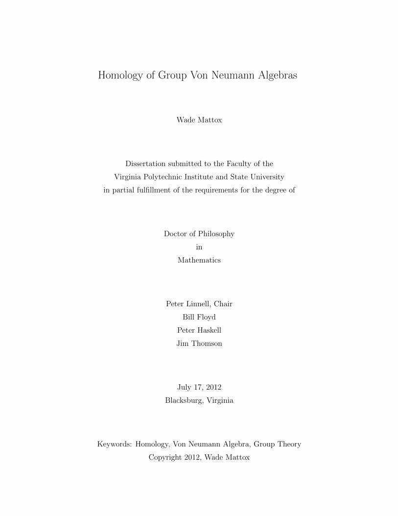
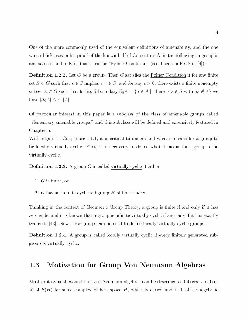
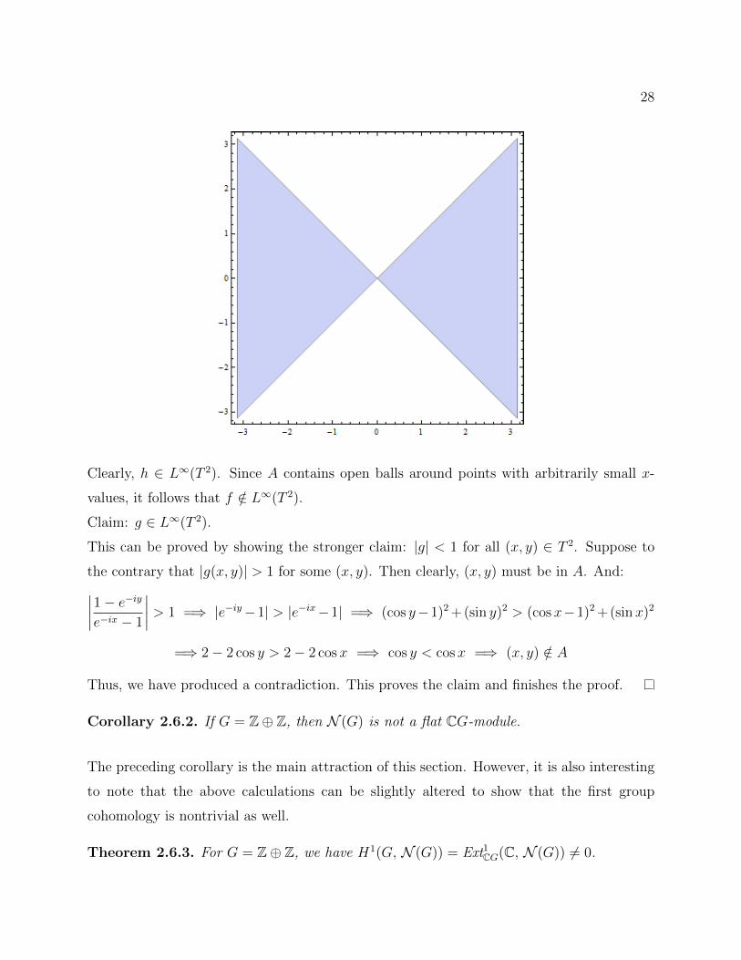
Define A = (x, y) ∈ T 2 : cos y > cosx, and let h = χA. The region A is pictured below:

28

Clearly, h ∈ L∞(T 2). Since A contains open balls around points with arbitrarily small x-

values, it follows that f /∈ L∞(T 2).

Claim: g ∈ L∞(T 2).

This can be proved by showing the stronger claim: |g| < 1 for all (x, y) ∈ T 2. Suppose to

the contrary that |g(x, y)| > 1 for some (x, y). Then clearly, (x, y) must be in A. And:∣∣∣∣1− e−iye−ix − 1

∣∣∣∣ > 1 =⇒ |e−iy−1| > |e−ix−1| =⇒ (cos y−1)2 +(sin y)2 > (cosx−1)2 +(sinx)2

=⇒ 2− 2 cos y > 2− 2 cosx =⇒ cos y < cosx =⇒ (x, y) /∈ A

Thus, we have produced a contradiction. This proves the claim and finishes the proof.

Corollary 2.6.2. If G = Z⊕ Z, then N (G) is not a flat CG-module.

The preceding corollary is the main attraction of this section. However, it is also interesting

to note that the above calculations can be slightly altered to show that the first group

cohomology is nontrivial as well.

Theorem 2.6.3. For G = Z⊕ Z, we have H1(G, N (G)) = Ext1CG(C, N (G)) 6= 0.

29

Proof. We want to calculate H1(G,N (G)) = Ext1CG(C,N (G)). We can reuse some of the

work from the last proof. Take the same resolution of C as above (since G is abelian we

don’t have to worry about the difference between left-actions and right-actions). Now apply

the functor HomCG(−,N (G)). This yields the complex:

0→ HomCG(CG,L∞(T 2))β∗−→ HomCG(CG2, L∞(T 2))

γ∗−→ HomCG(CG,L∞(T 2))→ 0,

which becomes:

0→ L∞(T 2)β∗−→ L∞(T 2)2 γ∗−→ L∞(T 2)→ 0,

where β∗ : f 7→ ((e−ix − 1)f, (e−iy − 1)f), and γ∗ : (g, h) 7→ (1 − e−iy)g + (e−ix − 1)h. We

would like to find an element of ker (γ∗) which is not in Im(β∗). Suppose (G,H) ∈ ker (γ∗).

Then (1 − e−iy)G + (e−ix − 1)H = 0. And suppose (G,H) ∈ Im(β∗). Then there exists

F ∈ L∞(T 2) such that G = (e−ix− 1)F and H = (e−iy − 1)F . So it suffices to construct the

following scenario:

G ∈ L∞(T 2), F =G

e−ix − 1/∈ L∞(T 2), H =

(1− e−iy)G−(e−ix − 1)

∈ L∞(T 2).

Using the f, g, h as defined in the previous proof, it is clear that if G = h ∈ L∞(T 2), then

F = f /∈ L∞(T 2) and H = −g ∈ L∞(T 2).

It may be an interesting question to consider for which groups H1(G,N (G)) vanishes. We

have already seen that this cohomology group is trivial for G = Z, and it is nontrivial for

G = Z⊕ Z.

Finally, we would like to show that the modules `p(G) are also not flat over CG. In this

case, we do not have Fourier transforms at our disposal. However, since elements of `p(G)

are easier to identify than elements of N (G), the transforms are not needed for this proof.

Theorem 2.6.4. Let G = Z⊕ Z and 1 ≤ p ∈ R. Then H1(G, `p(G)) 6= 0.

Proof. We can use the same free CG-resolution as before:

0→ CG f−→ CG2 k−→ CG ε−→ C→ 0,

30

where f : x =∑an,m · tnsm 7→ (−(s− 1)x, (t− 1)x),

and k : (x, y) 7→ (t − 1)x + (s − 1)y, for G = 〈t, s | ts = st〉. Now apply the functor

`p(G)⊗CG − to obtain the following deleted complex:

0→ `p(G)f∗−→ `p(G)2 k∗−→ `p(G)→ 0,

where f∗ : x 7→ (−(s − 1)x, (t − 1)x) and k∗ : (x, y) 7→ (t − 1)x + (s − 1)y. It suffices to

find (α, β) ∈ ker (k∗) such that (α, β) /∈ Im(f∗). So it suffices to find α, β ∈ `p(G) such that

(t − 1)α = (s − 1)β but there does not exist γ ∈ `p(G) such that α = (s − 1)γ. Use the

following notation:

α =∑g∈G

ag · g, β =∑g∈G

bg · g, γ =∑g∈G

cg · g.

Assume α(t− 1) = β(s− 1). Then (∑ag · g) (t− 1) = (

∑bg · g) (s− 1), which implies:(∑

ag · gt)−(∑

ag · g)

=(∑

bg · gs)−(∑

bg · g),∑

(agt−1 − ag) · g =∑

(bgs−1 − bg) · g.

Hence, for all g ∈ G, agt−1−ag = bgs−1−bg. Solve this equation for bg: bg = (ag−agt−1)+bgs−1 .

Substituting this equation into itself repeatedly yields the following relationship between the

β coefficients and the α coefficients:

bg =∞∑k=0

(ags−k − ags−kt−1

). (2.1)

Now assume that α = γ(s− 1). Then:∑ag · g =

(∑cg · g

)(s− 1) =

(∑cg · gs

)−(∑

cg · g)

=∑

(cgs−1 − cg) · g.

Therefore, ag = cgs−1 − cg for all g ∈ G, and cg = −ag + cgs−1 . As before, this leads to a

relationship between the γ coefficients and the α coefficients:

cg = −∞∑k=0

ags−k . (2.2)

Let r ∈ R be such that (m + n)−r ∈ `p(N × N) and (m + n)−r+1 /∈ `p(N × N). For

g = smtn, denote ag with am,n. First define a0,n = 0 for all n ∈ Z. Next define the “first

31

quadrant” of α coefficients. For m > 0 and n ≥ 0, define am,n = (m + n)−r. Next define

the “fourth quadrant” of α coefficients. For m ≥ 0 and n < 0, define am,n = am,−n. Finally,

define the second and third quadrants of α coefficients. For m < 0 and n ∈ Z, define

am,n = −a−m,n. By the choice of r, it follows that α ∈ `p(G). For m < 0 and n > 0:

cm,n = −−∞∑k=m

ak,n =∞∑

k=−m

ak,n =∞∑

k=−m

1

(k + n)r= Θ((−m+ n)−r+1).

By the choice of r, it follows that γ /∈ `p(G). Now consider β. Note that for m,n ≥ 1,

(m + n)−r − (m + n − 1)−r = Θ((m + n)−r−1), with respect to the variable n. Hence, for

m < 0 and n > 0:

bm,n =−∞∑k=m

(ak,n − ak,n−1) = −∞∑

k=−m

(ak,n − ak,n−1)

= −∞∑

k=−m

(k + n)−r − (k + n− 1)−r = −∞∑

k=−m

Θ((k + n)−r−1) = Θ((−m+ n)−r).

For the other three quadrants, the bounds of bg are similar. Hence, by the choice of r, it

follows that β ∈ `p(G).

2.7 Group C∗-algebras

Another class of operator algebras, similar to von Neumann algebras, is the class of C∗-

algebras. An example of a prototypical C∗-algebra is a subset X of B(H) for some complex

Hilbert space H, which is closed under all of the algebraic operations on B(H) (addition,

multiplication, scalar multiplication), is closed with respect to the norm topology, and is

closed under the adjoint operation. More generally, a C∗-algebra is defined as follows.

Definition 2.7.1. A C∗-algebra is a complex Banach algebra (with a unit element I) with

an involution that is closed under the norm topology.

Since the norm topology is stronger than the weak topology, it follows that any von Neumann

algebra is also a C∗-algebra. For a group G there are a couple of relevant C∗-algebras (which

are in general not von Neumann algebras) associated to G, and the questions being asked

about N (G) in this paper can also be asked about these other algebras.

32

First, let’s define what is called a “reduced group C∗-algebra,” denoted C∗r (G), for a

group G. Consider the left regular representation λ : G → B(`2(G)), where for any x ∈ G,

λ(x) : `2(G)→ `2(G) maps∑g∈G

ag · g to∑g∈G

ax−1g · g. This induces a representation of `1(G),

λ : `1(G) → B(`2(G)) ( [9], p. 183). For any A =∑g∈G

ag · g ∈ `1(G), define λ(A) to be

the map

(∑g∈G

ag · λ(g)

): `2(G)→ `2(G). Then the reduced group C∗-algebra is the norm-

closure of all such operators on `2(G); C∗r (G) = λ(`1(G)). Another algebra associated to G is

one called the “group C∗-algebra,” denoted C∗(G). Define it to be the enveloping C∗-algebra

of `1(G). Much like N (G), these group C∗-algebras were originally studied in the context

of Representation Theory of infinite groups (see [24], section 10.3). In general, C∗r (G) is a

quotient of C∗(G). However, if G is amenable, then C∗(G) ∼= C∗r (G) ( [9], Theorem VII.2.5).

Just as with N (G), it can be easier to work with C∗r (G) when G is abelian. This is because

one may work within the context of the dual group, as the next theorem describes ( [9],

Proposition VII.1.1).

Theorem 2.7.2. If G is an abelian group, then C∗(G) ∼= C∗r (G) ∼= C0(Γ), where Γ is the

dual group of G and C0(Γ) is the space of all continuous functions on Γ vanishing at infinity.

This fact allows us to mimic the group homology and cohomology calculations done earlier

for G = Z and G = Z⊕ Z. For G = Z, we can use the dual group, and the proof works out

analogously to how it did in section 2.4.

Theorem 2.7.3. If G = Z and M = C∗(G) = C∗r (G), then H1(G, M) = 0 and H1(G, M) =

0.

Proof. Let G = 〈t〉 ∼= Z. Take the standard free CG-resolution of C:

0→ CG f−→ CG ε−→ C→ 0,

where ε is the augmentation map and f is multiplication by t − 1 on the right. Now apply

−⊗CGM to create the complex:

0→Mf∗−→M → 0,

33

where f∗ is still multiplication by t−1. To show H1(G, M) = 0 it suffices to show the kernel

of f∗ is trivial. Convert everything into the context of the dual group Γ ∼= S1:

0→ C0(S1)f∗−→ C0(S1)→ 0,

where f∗ is multiplication on the left by the function e−ix−1. Since e−ix−1 vanishes only on

a set of measure 0, if it is multiplied against any other function with support of full measure,

the result will also be a function that vanishes only on a set of measure 0. In other words,

the kernel of f∗ is trivial. Hence, H1(G, M) = 0. Similarly, H1(G, M) = 0.

For G = Z⊕Z, we can again use the dual group, except we must use a continuous analogue

of the characteristic function which was used in section 2.5.

Theorem 2.7.4. If G = Z ⊕ Z and M = C∗(G) = C∗r (G), then H1(G, M) 6= 0 and

H1(G, M) 6= 0.

Proof. Let G = 〈s, t | ts = st〉 ∼= Z⊕ Z. Build a free CG-resolution of C:

0→ CG γ−→ CG2 β−→ CG ε−→ C→ 0,

where γ : x =∑an,m · tnsm 7→ (−(s− 1)x, (t− 1)x),

and β : (x, y) 7→ (t− 1)x+ (s− 1)y, for G = 〈t, s | ts = st〉.Next apply the functor N (G)⊗− to obtain a deleted complex:

0→ C0(T 2)γ′−→ C0(T 2)2 β′−→ C0(T 2)→ 0,

where γ′ : f 7→ (f · (1− e−iy), f · (e−ix − 1)),

and β′ : (g, h) 7→ g · (e−ix − 1) + h · (e−iy − 1).

Now we are ready to calculate the first group homology: H1(G, M) ∼= ker (β′)/Im(γ′).

Suppose (g, h) ∈ ker (β′). Then g · (e−ix − 1) + h · (e−iy − 1) = 0. Define

f =g

1− e−iy=

h

e−ix − 1.

The group homology vanishes if every such f must be in C0(T 2). We can show that the

group homology is nontrivial if there exists (g, h) ∈ ker (β′) such that f /∈ C0(T 2). In other

34

words, we need to create the following situation:

h ∈ C0(T 2), f =h

e−ix − 1/∈ C0(T 2), g =

h · (1− e−iy)e−ix − 1

∈ C0(T 2).

Just as in section 2.5, define A = (x, y) ∈ T 2 : cos y > cosx. This time let h(x, y) be

a continuous function with support contained in A such that h(x, 0) =√|x|. I claim that

g ∈ C0(T 2). First, we want to show that |g| < d for all (x, y) ∈ T 2, where d = ||h||∞.

Suppose to the contrary that |g(x, y)| > d for some (x, y). Then clearly, (x, y) must be in A.

And:∣∣∣∣1− e−iye−ix − 1

∣∣∣∣ > 1 =⇒ |e−iy−1| > |e−ix−1| =⇒ (cos y−1)2 +(sin y)2 > (cosx−1)2 +(sinx)2

=⇒ 2− 2 cos y > 2− 2 cosx =⇒ cos y < cosx =⇒ (x, y) /∈ A.

Thus, we have produced a contradiction. Hence g is bounded. Since g is a bounded quotient

of continuous functions, g must be measurably equivalent to a continuous function. To show

the group homology is nontrivial, it now suffices to show f /∈ C0(T 2). This is true since:

limx→0+

|f(x, 0)| = limx→0+

∣∣∣∣ h(x, 0)

e−ix − 1

∣∣∣∣ = limx→0+

∣∣∣∣ √xe−ix − 1

∣∣∣∣ = limx→0+

∣∣∣∣ 1

2√xe−ix

∣∣∣∣ =∞.

Hence, f cannot be extended to be a continuous function, and H1(G, M) 6= 0.

Similarly, H1(G, M) 6= 0.

It may be an interesting question to consider for which groups G the CG-module C∗(G) is

flat.

2.8 Connections: N (G), U(G), and `2(G)

The results of this section will be critical for taking the calculations for special cases such

as Z and Z ⊕ Z and drawing conclusions about wider classes of groups. Perhaps the most

important such result is the following connection between groups and subgroups ( [31],

Theorem 6.29(1)).

Theorem 2.8.1. If H ≤ G and N (G) is flat over CG, then N (H) is flat over CH.

35

The contrapositive of the previous theorem will be utilized extensively in this paper:

Corollary 2.8.2. If H ≤ G and N (H) is not flat over CH, then N (G) is not flat over CG.

For example, if we combine this fact with (2.6.2), then we get the next result.

Corollary 2.8.3. If G contains a subgroup isomorphic to Z⊕Z, then N (G) is not flat over

CG.

There is an analogous relationship between groups and subgroups with respect to the CG-

module `p(G).

Theorem 2.8.4. Let 1 ≤ p ∈ R. If H ≤ G and `p(G) is flat over CG, then `p(H) is flat

over CH.

Proof. The first relevant fact is that `p(H) is a summand of `p(G) as CH-modules. Indeed, let

X be a transversal for H in G, and assume 1 ∈ X. Then `p(G) = `p(H)⊕

( ∐16=x∈X

x`p(H)

).

Rewrite this as `p(G) = `p(H) ⊕ Y . Now let E be an exact sequence of CH-modules

0 → A → B → C → 0. Since CG is flat over CH, E ⊗CH CG is an exact sequence of CG-

modules. Since `p(G) is flat over CG, E ⊗CH `p(G) is an exact sequence of `p(G)-modules.

But E⊗CH `p(G) ∼= (E⊗CH `

p(H))⊕ (E⊗CH Y ) is exact implies that E⊗CH `p(H) is exact.

Therefore `p(H) is flat over CH.

Hence, we have the following corollary, which is a useful tool for classifying for which groups

G `2(G) is not flat over CG.

Corollary 2.8.5. Let 1 ≤ p ∈ R. If H ≤ G and `p(H) is not flat over CH, then `p(G) is

not flat over CG.

So, loosely speaking, non-flatness with respect to a subgroup implies non-flatness with respect

to the group. In general, the converse is not true (e.g., G = Z ⊕ Z and H = Z). However,

the converse is true if H is a subgroup of finite index. This fact is based on the following

identity.

36

Lemma 2.8.6. Suppose H ≤ G and M(G) = N (G) or M(G) = `p(G) for some 1 ≤ p ∈ R.

If [G : H] <∞, then M(G) ∼= M(H)⊗CH CG as right CG-modules.

Proof. Let [g1, g2, . . . , gn] be a transversal of G with respect to H. For any g ∈ G, let hg ∈ Hbe such that g = hggi for some i ∈ [1, 2, . . . , n]. Define Xi to be the set of all g ∈ G which

are in the orbit of gi. Define a CG-map ϕ : M(G)→M(H)⊗CH CG as follows:

∑g∈G

ag · g 7→n∑i=1

((∑g∈Xi

ag · hg

)⊗ gi

).

And define another CG-map ψ : M(H)⊗CH CG→M(G) by α⊗ β 7→ αβ. Then ψϕ = id:

∑g∈G

ag · gϕ7→

n∑i=1

((∑g∈Xi

ag · hg

)⊗ gi

)ψ7→

n∑i=1

(∑g∈Xi

ag · hggi

)=∑g∈G

ag · g.

Now let α =∑h∈H

ag · h ∈M(H) and g ∈ G. Suppose g = hggi. By linearity, to show ϕψ = id

it suffices to show ϕψ(α⊗ g) = α⊗ g. This is true because of the following calculation:

ψ(α⊗g) = αg =∑h∈H

ah·hg =∑h∈H

ah·hhggiϕ7→

(∑h∈H

ah · hhg

)⊗gi =

(∑h∈H

ah · h

)⊗hggi = α⊗g.

Hence, ϕ is an isomorphism, and the result follows.

Using the previous lemma, we can prove a relationship between groups and subgroups of

finite index.

Proposition 2.8.7. Suppose H ≤ G and M(G) = N (G) or M(G) = `p(G) for some

1 ≤ p ∈ R. If [G : H] < ∞, and M(H) is a flat CH-module, then M(G) is a flat CG-

module.

Proof. Because of (2.8.6), the functor M(G) ⊗CG − is the composition of the functors

M(H)⊗CH − and CG⊗CG −, which are both exact by hypothesis.

37

In general, there aren’t any analogous results for groups with respect to quotient groups.

However, if the quotient group is obtained by factoring out a finite normal subgroup, then

there are some nice results.

Theorem 2.8.8. Let H be a finite normal subgroup of G, and let Q = G/H. Let M(G) =

`p(G) for some 1 ≤ p ∈ R or M(G) = N (G). If M(G) is flat over CG, then M(Q) is flat

over CQ.

Proof. The first relevant claim is that M(Q) is a summand of M(G) as CG-modules. Con-

sider the following central idempotent element of M(G): e =1

|H|∑h∈H

h. Since e is a central

idempotent, it follows that M(G) ∼= M(G)e ⊕M(G)(1 − e). So to prove the first claim, it

suffices to show M(Q) ∼= M(G)e. Let X = xi be a transversal in G with respect to H.

And define ϕ : M(Q) → M(G)e by∑ai · xi 7→

∑ai · xie. It is clear that ϕ is an injective

homomorphism. It remains to show ϕ is surjective. Pick an arbitrary element α ∈ M(G)e.

Then α can be written as∑cij · hixje, where H = hiNi=1. Note that hixje = hkxje = xje

for all i, k ∈ 1, 2, . . . , N. Hence α =∑j

(N∑i=1

cij

)xje and we see that a pre-image for α is

∑j

(N∑i=1

cij

)xj. This proves that M(Q) is a summand of M(G). Write M(G) ∼= M(Q)⊕P .

Now let E : 0 → A → B → C → 0 be an exact sequence of CQ-modules. By assumption,

the sequence E ⊗CG M(G) must be exact. But since M(G) ∼= M(Q) ⊕ P , we can rewrite

this short exact sequence as (E⊗CGM(Q))⊕ (E⊗CG P ). It follows that E⊗CGM(Q) must

be exact. And since the action of H is trivial on all modules in this sequence, it follows that

E⊗CQM(Q) is exact.

There is also a relationship between homology groups, which requires a lemma.

Lemma 2.8.9. Let H be a finite normal subgroup of G, and let Q = G/H. Then there is a

CQ-module isomorphism `p(G)H ∼= `p(Q).

Proof. Since H is finite, there is a natural surjective CG-homomorphism ϕ : `p(G)→ `p(Q).

And ∆(H)`p(G) ⊆ kerϕ, and so this induces a map ϕ : `p(G)∆(H)`p(G)

→ `p(Q). Claim: ϕ is

38

injective. Let R = gi be a set of coset representatives in G with respect to H. Suppose

x =∑a(g) · g ∈ `p(G) and [x] 7→ 0. Then

∑a(g) · g = 0 and hence

∑h∈H

a(hgi) = 0 for every

gi ∈ R. Now we can use this fact to show that [x] = 0:

[x] =

[∑H

∑R

a(hgi) · hgi

]=∑H

[h∑R

a(hgi)gi

]=∑H

[∑R

a(hgi)gi

]=

[∑R

(∑H

a(hgi)

)gi

]= 0.

Therefore ϕ is a CG-isomorphism. Since the H-action is trivial on both the domain and

codomain of ϕ, it follows that ϕ is a CQ-isomorphism.

Using the previous lemma, we get the following relationship between group homology over

G and group homology over Q.

Theorem 2.8.10. Let H be a finite normal subgroup of G, and let Q = G/H. Then

H1(G, `p(G)) ∼= H1(Q, `p(Q)).

Proof. The short exact sequence of groups 1 → H → G → Q → 1 induces the following

exact sequence on homology:

H2(G, `p(G))→ H2(Q, `p(G)H)→ H1(H, `p(G))Q → H1(G, `p(G))→ H1(Q, `p(G)H)→ 0.

Since H is finite, it follows that H1(H, `p(G)) = 0, and hence H1(G, `p(G)) ∼= H1(Q, `p(G)H).

The result now follows from the previous lemma.

Next, we would like to show that there is a relationship between whether N (G) is flat over

CG and whether `2(G) is flat over CG. The first necessary lemma for this states, in effect,

that N (G) is always a semi-hereditary ring ( [31], Theorem 6.7(1)).

Lemma 2.8.11. Any finitely generated submodule of a projective N (G)-module is projective.

And since N (G) is semi-hereditary, submodules of free modules must be flat.

Lemma 2.8.12. Any submodule of a free N (G)-module is flat.

39

Proof. Let M be a submodule of a free N (G)-module. Then M can be expressed as a direct

limit of its finitely generated submodules, which each must be projective by the previous

lemma. Since M is a direct limit of projective modules, it must be a flat module.

The final lemma necessary to show the relationship between `2(G) and N (G) is:

Lemma 2.8.13. The N (G)-module U(G) can be written as a direct limit (and a union) of

free modules Fα for which every Fα ∼= N (G).

Proof. Let X = α ∈ N (G) | α is a non-zero-divisor. For α ∈ X, define Fα = α−1N (G),

which is a submodule of U(G) and a free N (G)-module. Then U(G) =⋃α∈X

Fα. To show

this union is also a direct limit, it suffices to show that Fα is a direct system. In other

words, for every pair of non-zero-divisors α, β, we want to show there is a cofinal Fγ such

that Fα ⊆ Fγ and Fβ ⊆ Fγ. Since N (G) satisfies the Ore condition, there exists δ, y ∈ N (G)

such that δ is a non-zero-divisor and δβ = yα. Hence, for any α−1x ∈ α−1N (G) we have:

α−1x = β−1βα−1x = (β−1δ−1)yx ∈ (δβ)−1N (G)

And for any β−1x ∈ β−1N (G) we have:

β−1x = β−1δ−1δx ∈ (δβ)−1N (G)

Therefore, defining γ = δβ provides the cofinal Fγ that we required.

Now we are ready to prove the important fact about `2(G) as a module over N (G).

Theorem 2.8.14. Let G be a group. Then `2(G) is a flat N (G)-module.

Proof. By the preceding lemma, express U(G) as⋃Fα, which is a direct limit of free modules

of rank one. Since `2(G) can be imbedded in U(G), it can be thought of as a submodule.

Hence:

`2(G) = U(G) ∩ `2(G) =(⋃

Fi

)∩ `2(G) =

⋃(Fi ∩ `2(G)

)Note that Fα∩`2(G) is a flat module by (2.8.12). Hence `2(G) is a direct limit of flat modules

and the result follows.

40

In particular, this leads to the next corollary, which will be relied upon heavily in Chapter

4.

Corollary 2.8.15. If N (G) is flat over CG, then `2(G) is flat over CG.

The previous Corollary stated that to show N (G) is not flat over CG, it suffices to show

`2(G) is not flat over CG. As it turns out, N (G) has the same relationship with U(G), on

account of U(G) being the Ore localization of N (G) ( [44], Proposition II.1.4).

Theorem 2.8.16. The algebra of affiliated operators U(G) is flat over N (G).

Corollary 2.8.17. If U(G) is not flat over CG, then N (G) is not flat over CG.

2.9 The Case G = Z ∗ Z

Next we want to consider the free group on two generators G = Z ∗ Z. Before calculating

the group homology for this group, we will need the following lemma ( [31], Lemma 6.36).

Lemma 2.9.1. Let G be a group, and let H be a subgroup of G. Then N (G)⊗CG C[G/H]

is trivial if and only if H is non-amenable.

With this lemma in mind, it is relatively straightforward to show the first group homology is

nontrivial. In fact, one can show the von Neumann dimension of the homology group (i.e.,

the first L2-Betti number) is nontrivial.

Theorem 2.9.2. If G = Z ∗ Z and M = N (G), then dimN (G) (H1(G, M)) 6= 0.

Proof. Recall the free CG resolution of C: 0 → CG2 → CG → C → 0. Now apply the

functor N (G) ⊗CG −, which is always right exact: N (G)2 → N (G) → N (G) ⊗CG C → 0.

By 2.9.1, N (G) ⊗CG C = 0 since Z ∗ Z is not amenable. Thus we have the exact sequence:

N (G)2 → N (G)→ 0. Now H1(G, M) is just the kernel of this map, which has von Neumann

dimension one by additivity (see 1.5.4).

41

This implies that for G = Z∗Z, the group von Neumann algebra is neither flat nor dimension-

flat over CG. By 2.8.2, for any group G with Z∗Z as a subgroup, N (G) is not flat over CG.

We would like to go one step further and say that for such groups N (G) is not dimension-flat.

Before that can be proved, we need two lemmas.

Lemma 2.9.3. For any subgroup H ≤ G and any CH-module M we have:

N (G)⊗N (H) TorCH1 (N (H), M) ∼= TorCG1 (N (G), CG⊗CH M).

Proof. Since N (G) is flat over N (H),

N (G)⊗N (H) TorCH1 (N (H), M) ∼= TorCH1 (N (G), M).

This last Tor-group can be calculated by taking a projective CH-resolution P of M , applying

the functor N (G) ⊗CH −, and taking homology. But since N (G) ∼= N (G) ⊗CG CG, it is

equivalent to apply the functor N (G)⊗CGCG⊗CH− to P. And this is equivalent to applying

the functor N (G)⊗CG − to CG⊗CH P, which is a projective CG-resolution of CG⊗CH M

since CG is a free CH-module (see [7], exercise I.3.1). Hence, the homology of the resulting

complex is isomorphic to TorCG1 (N (G), CG⊗CH M).

The next lemma, which can be found in [31] (Theorem 6.29(2)), provides a strong relationship

between the dimensions of a module and its induced module.

Lemma 2.9.4. Let H be a subgroup of G, and let M be any N (H)-module. Then dimN (G)(N (G)⊗N (H)

M) = dimN (H)(M).

Now we can prove the lack of dimension-flatness for any group containing a non-abelian free

subgroup.

Proposition 2.9.5. Let G be a group with a subgroup isomorphic to Z ∗ Z. Then N (G) is

not dimension-flat over CG.

Proof. Let H ∼= Z ∗ Z ≤ G. Then, by 2.9.2, dimN (H)

(TorCH1 (N (H),C)

)= 1. By 2.9.3,

N (G)⊗N (H) TorCH1 (N (H),C) ∼= TorCG1 (N (G),CG⊗CH C). By 2.9.4, it follows that:

dimN (G)

(TorCG1 (N (G),CG⊗CH C)

)= dimN (G)

(N (G)⊗N (H) TorCH1 (N (H),C)

)

42

= dimN (H)

(TorCH1 (N (H),C)

)= 1.

This result, due to Luck, proves that Conjecture A is true for any group which contains

Z ∗ Z as a subgroup, since all such groups are non-amenable ( [37], Example 0.6). However,

Conjecture A is still open in general, since there exist non-amenable groups which do not

have any nonabelian free subgroups [35].

Chapter 3

Proving Half of Conjecture B

3.1 Introduction

In this chapter, the first half of Conjecture 1.1.1 will be proved. In other words, we will

prove that if a group G is locally virtually cyclic, then N (G) is a flat CG-module. First,

special cases of locally virtually cyclic groups will be considered: finite groups and infinite

locally finite groups. Then the focus will be shifted to locally virtually cyclic groups with

elements of infinite order. The most foundational case, of course, will be the infinite cyclic

group G = Z. This case will serve as a stepping stone to the case when G is virtually

cyclic. Finally, the jump can be made from virtually cyclic groups to locally virtually cyclic

groups, thereby proving half of Conjecture 1.1.1. The final step to proving the result for

locally virtually cyclic groups will require demonstrating that certain Tor-groups vanish,

and this will be accomplished by first converting the Tor calculations into group homology

calculations. Then the proof can be completed by using previous results and a few important

facts about group homology with respect to subgroups and direct limits.

43

44

3.2 Locally Finite Groups

In this section, we will show that Conjecture 1.1.1 is consistent for the class of finite groups

and infinite locally finite groups. First, suppose that G is a finite group. Then CG =

N (G) = `2(G). This implies that N (G) is a free CG-module, and hence it is flat. When G is

locally finite, then N (G) may not be a free module. However, we can show that it must be a

flat module just by looking at the ring CG. In particular, it is known that every CG-module

is flat. This can be realized as the corollary of some classical results in Ring Theory. First,

recall what a semisimple module is.

Definition 3.2.1. An R-module M is simple if it has no nontrivial, proper submodules. We

call M semisimple if it is a direct sum of simple modules. A ring R is called semisimple if it

is semisimple as a module over itself.

The following theorem, called Maschke’s Theorem ( [1], p. 157), describes a sufficient con-

dition for a group ring to be semisimple.

Theorem 3.2.2. Let G be a finite group, and let k be a field whose characteristic does not

divide the order of G. Then the group ring kG is a semisimple ring.

And a version of the Artin-Wedderburn Theorem ( [1], p. 152) gives us a powerful fact about

semisimple rings.

Theorem 3.2.3. A ring R is semisimple if and only if every R-module is projective.

We will use the previous two theorems to show that CG is a so-called von Neumann regular

ring.

Definition 3.2.4. A ring R is von Neumann regular if for every a ∈ R, there exists x ∈ Rsuch that a = axa.

The definition above is the most classical way to define von Neumann regular rings. However,

it is the following characterization that will be most relevant for our purpose (see Theorem

4.2.9 in [47]).

45

Theorem 3.2.5. A ring R is von Neumann regular if and only if every R-module is flat.

These results provide the foundation for showing that every CG-module (and in particular,

N (G)) is flat for locally finite groups.

Theorem 3.2.6. If G is a locally finite group, then CG is a von Neumann regular ring.

Proof. To show CG is von Neumann regular, it suffices to show that for all x ∈ CG there

exists a ∈ CG such that axa = a. Let a = a1g1 + · · · + angn be an arbitrary element of

CG. Let H be the finite subgroup generated by g1, . . . , gn. Then a ∈ CH so it suffices

to show CH is von Neumann regular. And this follows from Maschke’s Theorem and the

Artin-Wedderburn Theorem, since projective modules are always flat modules.

This result is nothing new. However, it is interesting to note that I originally set out to prove

that N (G) is flat if and only if G is virtually cyclic. Infinite locally finite groups provided

the first example of groups for which N (G) is flat but G is not virtually cyclic, and so the

conjecture had to be revised to include all locally virtually cyclic groups.

3.3 Locally Virtually Cyclic Groups

Now let us reconsider the case G = Z. It was previously shown in 2.5.1 that H1(G, N (G)) =

0. Now we would like to go one step further and prove that N (G) is flat over CG. First, a

basic fact about modules over Principal Ideal Domains is relevant.

Lemma 3.3.1. Let R be a PID, and let M be an R-module. If M is R-torsion-free, then

M is a flat R-module.

Proof. Consider M as the direct limit of its finitely generated submodules, M ∼= lim−→Mi.

Since M is R-torsion-free, it must be the case that every Mi is R-torsion-free. By the

standard structure theorem for finitely generated modules over a PID ( [11], Theorem 12.1.5),

it follows that each Mi is a free R-module. Since M is a direct limit of free modules, it must

be a flat module.

46

Theorem 3.3.2. Let G = Z, and let M = N (G) or M = `p(G) for any 1 ≤ p ∈ R. Then

M is a flat CG-module.

Proof. For G = Z, the ring CG is a PID (see Corollary 6.4 in [21]). By the previous lemma, it

suffices to show M is R-torsion-free. But this is true by the Zero Divisor Conjecture [39].

As a result of 2.8.7, we have the following corollary.

Corollary 3.3.3. Suppose G is virtually cyclic, and let M = N (G) or M = `p(G) for any

1 ≤ p ∈ R. Then M is a flat CG-module.

The final necessary fact before proving half of Conjecture B is the following version of the

Zero Divisor Conjecture.

Lemma 3.3.4. Suppose G has a subgroup H such that H ∼= Z, and let 1 ≤ p ∈ R. Then

0 6= α ∈ CH and 0 6= β ∈ `p(G) implies that αβ 6= 0.

Proof. Let 0 6= α ∈ CH and 0 6= β ∈ `p(G). Let T be a transversal for H in G. Then

β =∑t∈T

αtt for some αt ∈ `p(H). Suppose, to the contrary, that αβ = 0. Then αβ =

α∑

t∈T αtt =∑

t∈T (ααt) t = 0 if and only if ααt = 0 for all t ∈ T if and only if αt = 0 for

all t ∈ T (by the Zero Divisor Conjecture being true for Z; see [39]) if and only if β = 0; a

contradiction. Therefore, αβ 6= 0.

Now we are ready to prove half of Conjecture B.

Theorem 3.3.5. Suppose G is locally virtually cyclic, and let M = N (G) or M = `p(G) for

any 1 ≤ p ∈ R. Then M is a flat CG-module.

Proof. Let B be any CG-module. It suffices to show TorCG1 (M, B) = 0. Since G is locally

virtually cyclic, we can express G as a direct limit of virtually cyclic groups: G = lim−→Gi.

Now utilize 2.2.4 and 2.2.3:

TorCG1 (M, B) ∼= H1(G, M ⊗B) ∼= lim−→H1(Gi, M ⊗B).

47

So it suffices to show H1(Gi, M ⊗ B) = 0. If Gi is finite, then this is true because of

3.2.6. Suppose each Gi is infinite. Since Gi is infinite virtually cyclic, there must be a

normal infinite cyclic subgroup of finite index (see 7.1.6). In other words, we can write

1 → Ki → Gi → Qi → 1, where Ki∼= Z and Qi is finite. If N = M ⊗ B, then there is the

following exact sequence (2.2.2):

H2(Qi, NKi)→ H1(Ki, N)Qi

→ H1(Gi, N)→ H1(Qi, NKi).

Since Qi is finite we know that H2(Qi, NKi) ∼= H1(Qi, NKi

) ∼= 0, hence H1(Gi, N) ∼=H1(Ki, N)Qi

. Therefore it suffices to show thatH1(Ki, N) = 0. Rewrite this as TorCKi1 (M, B).

This must be trivial since CKi is a PID and since M does not have any CKi-torsion. This

completes the proof.

This proves Conjecture 1.1.1(A). The rest of this paper will be concerned with Conjecture

1.1.1(B).

Chapter 4

Baumslag-Solitar Groups

4.1 Introduction

One critical case for Conjecture 1.1.1(B), G = Z⊕Z, was considered in Chapter 2. Two more

critical cases will be considered in this chapter. The first case consists of a class of groups

called “Baumslag-Solitar groups.” These groups were introduced by Gilbert Baumslag and

Donald Solitar in 1962 to provide finitely-presented examples of Hopfian groups [3]; i.e.,

some of these groups have epimorphisms onto themselves which are not isomorphisms. These

groups are defined with the following presentation. For natural numbers m and n, define

B(m,n) = 〈a, b | abma−1 = bn〉. Since these groups are one-relator groups, we will use Fox

derivatives to do group homology calculations on them. If m 6= 1 and n 6= 1, then it can

be shown that B(m,n) has a copy of Z ∗ Z as a subgroup [8]. We shall look only at the

amenable Baumslag-Solitar groups, B(1, n). These groups are of cohomological dimension 2

( [5], Theorem 7). In fact, they are the only finitely-generated elementary amenable groups

with this property ( [25], Theorem 3). Another way of expressing B(1, n) is as a semi-direct

product.

Definition 4.1.1. Let G be a group with a normal subgroup H and a subgroup K. If

the natural embedding K → G composed with the natural projection G → G/H yields an

isomorphism K → G/H, then G = H oK is the semidirect product of H and K.

48

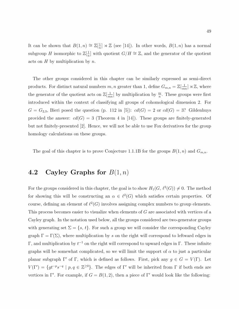
49

It can be shown that B(1, n) ∼= Z[ 1n] o Z (see [14]). In other words, B(1, n) has a normal

subgroup H isomorphic to Z[ 1n] with quotient G/H ∼= Z, and the generator of the quotient

acts on H by multiplication by n.

The other groups considered in this chapter can be similarly expressed as semi-direct

products. For distinct natural numbers m,n greater than 1, define Gm,n = Z[ 1mn

]oZ, where

the generator of the quotient acts on Z[ 1mn

] by multiplication by mn

. These groups were first

introduced within the context of classifying all groups of cohomological dimension 2. For

G = G2,3, Bieri posed the question (p. 112 in [5]): cd(G) = 2 or cd(G) = 3? Gildenhuys

provided the answer: cd(G) = 3 (Theorem 4 in [14]). These groups are finitely-generated

but not finitely-presented [2]. Hence, we will not be able to use Fox derivatives for the group

homology calculations on these groups.

The goal of this chapter is to prove Conjecture 1.1.1B for the groups B(1, n) and Gm,n.

4.2 Cayley Graphs for B(1, n)

For the groups considered in this chapter, the goal is to show H1(G, `2(G)) 6= 0. The method

for showing this will be constructing an α ∈ `2(G) which satisfies certain properties. Of

course, defining an element of `2(G) involves assigning complex numbers to group elements.

This process becomes easier to visualize when elements of G are associated with vertices of a

Cayley graph. In the notation used below, all the groups considered are two-generator groups

with generating set Σ = s, t. For such a group we will consider the corresponding Cayley

graph Γ = Γ(Σ), where multiplication by s on the right will correspond to leftward edges in

Γ, and multiplication by t−1 on the right will correspond to upward edges in Γ. These infinite

graphs will be somewhat complicated, so we will limit the support of α to just a particular

planar subgraph Γ′ of Γ, which is defined as follows. First, pick any g ∈ G = V (Γ). Let

V (Γ′) = gt−ps−q | p, q ∈ Z≥0. The edges of Γ′ will be inherited from Γ if both ends are

vertices in Γ′. For example, if G = B(1, 2), then a piece of Γ′ would look like the following:

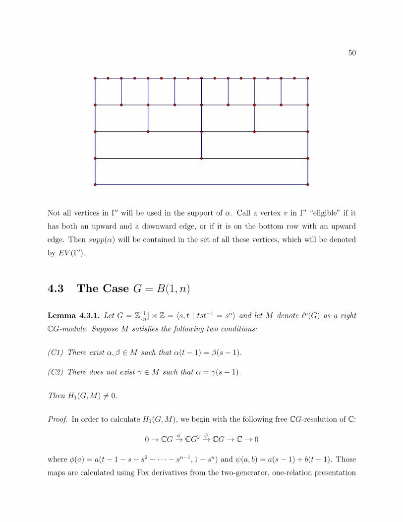
50

Not all vertices in Γ′ will be used in the support of α. Call a vertex v in Γ′ “eligible” if it

has both an upward and a downward edge, or if it is on the bottom row with an upward

edge. Then supp(α) will be contained in the set of all these vertices, which will be denoted

by EV (Γ′).

4.3 The Case G = B(1, n)

Lemma 4.3.1. Let G = Z[ 1n] o Z = 〈s, t | tst−1 = sn〉 and let M denote `p(G) as a right

CG-module. Suppose M satisfies the following two conditions:

(C1) There exist α, β ∈M such that α(t− 1) = β(s− 1).

(C2) There does not exist γ ∈M such that α = γ(s− 1).

Then H1(G,M) 6= 0.

Proof. In order to calculate H1(G,M), we begin with the following free CG-resolution of C:

0→ CG φ−→ CG2 ψ−→ CG→ C→ 0

where φ(a) = a(t− 1− s− s2 − · · · − sn−1, 1− sn) and ψ(a, b) = a(s− 1) + b(t− 1). Those

maps are calculated using Fox derivatives from the two-generator, one-relation presentation

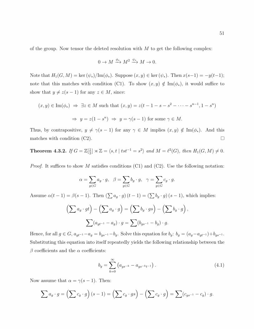
51

of the group. Now tensor the deleted resolution with M to get the following complex:

0→Mφ∗−→M2 ψ∗−→M → 0.

Note thatH1(G,M) = ker (ψ∗)/Im(φ∗). Suppose (x, y) ∈ ker (ψ∗). Then x(s−1) = −y(t−1);

note that this matches with condition (C1). To show (x, y) /∈ Im(φ∗), it would suffice to

show that y 6= z(s− 1) for any z ∈M , since:

(x, y) ∈ Im(φ∗) ⇒ ∃z ∈M such that (x, y) = z(t− 1− s− s2 − · · · − sn−1, 1− sn)

⇒ y = z(1− sn) ⇒ y = γ(s− 1) for some γ ∈M.

Thus, by contrapositive, y 6= γ(s − 1) for any γ ∈ M implies (x, y) /∈ Im(φ∗). And this

matches with condition (C2).

Theorem 4.3.2. If G = Z[12] o Z = 〈s, t | tst−1 = s2〉 and M = `2(G), then H1(G,M) 6= 0.

Proof. It suffices to show M satisfies conditions (C1) and (C2). Use the following notation:

α =∑g∈G

ag · g, β =∑g∈G

bg · g, γ =∑g∈G

cg · g.

Assume α(t− 1) = β(s− 1). Then (∑ag · g) (t− 1) = (

∑bg · g) (s− 1), which implies:(∑

ag · gt)−(∑

ag · g)

=(∑

bg · gs)−(∑

bg · g),∑

(agt−1 − ag) · g =∑

(bgs−1 − bg) · g.

Hence, for all g ∈ G, agt−1−ag = bgs−1−bg. Solve this equation for bg: bg = (ag−agt−1)+bgs−1 .

Substituting this equation into itself repeatedly yields the following relationship between the

β coefficients and the α coefficients:

bg =∞∑k=0

(ags−k − ags−kt−1

). (4.1)

Now assume that α = γ(s− 1). Then:∑ag · g =

(∑cg · g

)(s− 1) =

(∑cg · gs

)−(∑

cg · g)

=∑

(cgs−1 − cg) · g.

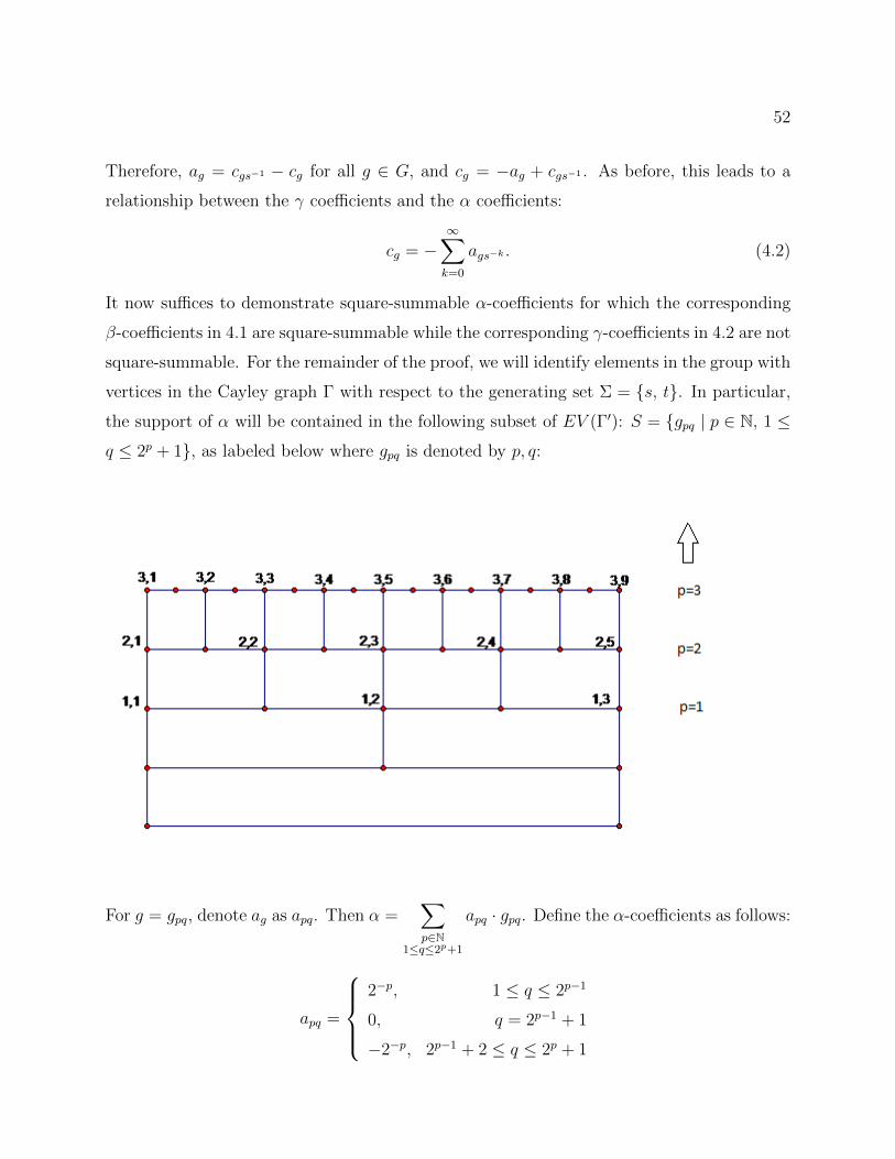
52

Therefore, ag = cgs−1 − cg for all g ∈ G, and cg = −ag + cgs−1 . As before, this leads to a

relationship between the γ coefficients and the α coefficients:

cg = −∞∑k=0

ags−k . (4.2)

It now suffices to demonstrate square-summable α-coefficients for which the corresponding

β-coefficients in 4.1 are square-summable while the corresponding γ-coefficients in 4.2 are not

square-summable. For the remainder of the proof, we will identify elements in the group with

vertices in the Cayley graph Γ with respect to the generating set Σ = s, t. In particular,

the support of α will be contained in the following subset of EV (Γ′): S = gpq | p ∈ N, 1 ≤q ≤ 2p + 1, as labeled below where gpq is denoted by p, q:

For g = gpq, denote ag as apq. Then α =∑p∈N

1≤q≤2p+1

apq · gpq. Define the α-coefficients as follows:

apq =

2−p, 1 ≤ q ≤ 2p−1

0, q = 2p−1 + 1

−2−p, 2p−1 + 2 ≤ q ≤ 2p + 1

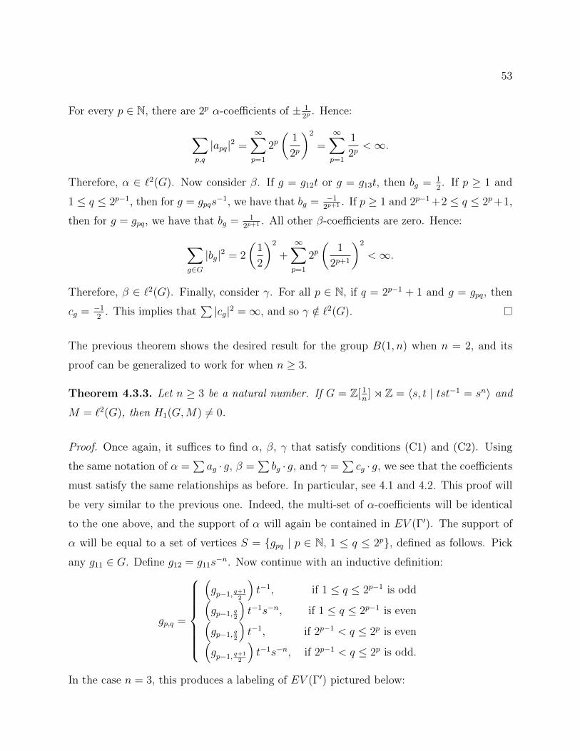
53

For every p ∈ N, there are 2p α-coefficients of ± 12p

. Hence:

∑p,q

|apq|2 =∞∑p=1

2p(

1

2p

)2

=∞∑p=1

1

2p<∞.

Therefore, α ∈ `2(G). Now consider β. If g = g12t or g = g13t, then bg = 12. If p ≥ 1 and

1 ≤ q ≤ 2p−1, then for g = gpqs−1, we have that bg = −1

2p+1 . If p ≥ 1 and 2p−1 +2 ≤ q ≤ 2p+1,

then for g = gpq, we have that bg = 12p+1 . All other β-coefficients are zero. Hence:

∑g∈G

|bg|2 = 2

(1

2

)2

+∞∑p=1

2p(

1

2p+1

)2

<∞.

Therefore, β ∈ `2(G). Finally, consider γ. For all p ∈ N, if q = 2p−1 + 1 and g = gpq, then

cg = −12

. This implies that∑|cg|2 =∞, and so γ /∈ `2(G).

The previous theorem shows the desired result for the group B(1, n) when n = 2, and its

proof can be generalized to work for when n ≥ 3.

Theorem 4.3.3. Let n ≥ 3 be a natural number. If G = Z[ 1n] o Z = 〈s, t | tst−1 = sn〉 and

M = `2(G), then H1(G,M) 6= 0.

Proof. Once again, it suffices to find α, β, γ that satisfy conditions (C1) and (C2). Using

the same notation of α =∑ag · g, β =

∑bg · g, and γ =

∑cg · g, we see that the coefficients

must satisfy the same relationships as before. In particular, see 4.1 and 4.2. This proof will

be very similar to the previous one. Indeed, the multi-set of α-coefficients will be identical

to the one above, and the support of α will again be contained in EV (Γ′). The support of

α will be equal to a set of vertices S = gpq | p ∈ N, 1 ≤ q ≤ 2p, defined as follows. Pick

any g11 ∈ G. Define g12 = g11s−n. Now continue with an inductive definition:

gp,q =

(gp−1, q+1

2

)t−1, if 1 ≤ q ≤ 2p−1 is odd(

gp−1, q2

)t−1s−n, if 1 ≤ q ≤ 2p−1 is even(

gp−1, q2

)t−1, if 2p−1 < q ≤ 2p is even(

gp−1, q+12

)t−1s−n, if 2p−1 < q ≤ 2p is odd.

In the case n = 3, this produces a labeling of EV (Γ′) pictured below:

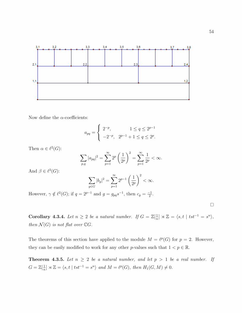
54

Now define the α-coefficients:

apq =

2−p, 1 ≤ q ≤ 2p−1

−2−p, 2p−1 + 1 ≤ q ≤ 2p.

Then α ∈ `2(G): ∑p,q

|apq|2 =∞∑p=1

2p(

1

2p

)2

=∞∑p=1

1

2p<∞.

And β ∈ `2(G): ∑g∈G

|bg|2 =∞∑p=1

2p−1

(1

2p

)2

<∞.

However, γ /∈ `2(G); if q = 2p−1 and g = gpqs−1, then cg = −1

2.

Corollary 4.3.4. Let n ≥ 2 be a natural number. If G = Z[ 1n] o Z = 〈s, t | tst−1 = sn〉,

then N (G) is not flat over CG.

The theorems of this section have applied to the module M = `p(G) for p = 2. However,

they can be easily modified to work for any other p-values such that 1 < p ∈ R.

Theorem 4.3.5. Let n ≥ 2 be a natural number, and let p > 1 be a real number. If

G = Z[ 1n] o Z = 〈s, t | tst−1 = sn〉 and M = `p(G), then H1(G,M) 6= 0.

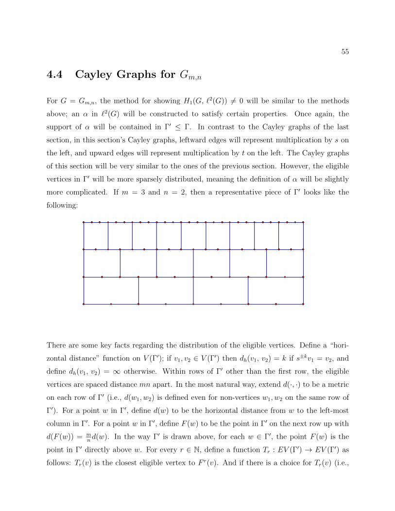
55

4.4 Cayley Graphs for Gm,n

For G = Gm,n, the method for showing H1(G, `2(G)) 6= 0 will be similar to the methods

above; an α in `2(G) will be constructed to satisfy certain properties. Once again, the

support of α will be contained in Γ′ ≤ Γ. In contrast to the Cayley graphs of the last

section, in this section’s Cayley graphs, leftward edges will represent multiplication by s on

the left, and upward edges will represent multiplication by t on the left. The Cayley graphs

of this section will be very similar to the ones of the previous section. However, the eligible

vertices in Γ′ will be more sparsely distributed, meaning the definition of α will be slightly

more complicated. If m = 3 and n = 2, then a representative piece of Γ′ looks like the

following:

There are some key facts regarding the distribution of the eligible vertices. Define a “hori-

zontal distance” function on V (Γ′); if v1, v2 ∈ V (Γ′) then dh(v1, v2) = k if s±kv1 = v2, and

define dh(v1, v2) = ∞ otherwise. Within rows of Γ′ other than the first row, the eligible

vertices are spaced distance mn apart. In the most natural way, extend d(·, ·) to be a metric

on each row of Γ′ (i.e., d(w1, w2) is defined even for non-vertices w1, w2 on the same row of

Γ′). For a point w in Γ′, define d(w) to be the horizontal distance from w to the left-most

column in Γ′. For a point w in Γ′, define F (w) to be the point in Γ′ on the next row up with

d(F (w)) = mnd(w). In the way Γ′ is drawn above, for each w ∈ Γ′, the point F (w) is the

point in Γ′ directly above w. For every r ∈ N, define a function Tr : EV (Γ′) → EV (Γ′) as

follows: Tr(v) is the closest eligible vertex to F r(v). And if there is a choice for Tr(v) (i.e.,

56

F r(v) is midway between two eligible vertices), choose the closest eligible vertex on the right

rather than left. For any w ∈ Γ′, denote the closest eligible vertex on the right by R(w).

In order to bound norms of elements in `2(G) later on, it will be helpful to consider

some bounds on distances in Γ′ presently. Note that for all w,w′ on the same row of Γ′,

d(F (w), F (w′)) = mnd(w,w′). And for all v ∈ EV (Γ′) and k ∈ N, d(F k(v), Tk(v)) ≤ mn.

It follows that d(Tk(v), tTk−1(v)) ≤ mn

(mn) + mn. Suppose that mn> 1, and let p be the

smallest natural number such that(mn

)p> 2. If v, v′ ∈ EV (Γ′) are such that d(v, v′) = mn

and v is to the left of v′, then d(Tp(v), Tp(v′)) > mn, which means there is another eligible

vertex between Tp(v) and Tp(v′). In this case, by the Triangle Inequality, the maximum

distance between any two of Tp(v), tTp−1(v), and R(Tp(v)) is mn

(mn) + 2mn. This constant

will be a useful bound, so give it a name; b = b(m,n) = mn

(mn) + 2mn. The notation of Tr,

R, p, and b as defined here will be utilized below.

4.5 The Case G = Gm,n

For some natural numbers m,n ≥ 2, let G = Gm,n = Z[ 1mn

] o Z, where the action on Z[ 1mn

]

is multiplication by mn

. Let M = `2(G), considered as a left CG-module. We would like to

show that H1(G, M) 6= 0. For notation, let H = Z[ 1mn

], which is a normal subgroup of G.

And let Q = G/H ∼= Z = 〈t〉. Let hi =(

1mn

)i, and define Hi = 〈hi〉 ≤ H. Then Hi

∼= Z and

H =⋃Hi.

Lemma 4.5.1. To prove that H1(G, M) 6= 0, it suffices to show H1(Q, MH) 6= 0.

Proof. There is the short exact sequence of groups 1 → H → G → Q → 1, which implies

there is an exact sequence on group homology:

H1(H, M)Q → H1(G, M)→ H1(Q, MH)→ 0.

And by (2.2.3):

H1(H, M) = H1

(lim−→Hi, M

) ∼= lim−→H1(Hi, M) = 0,

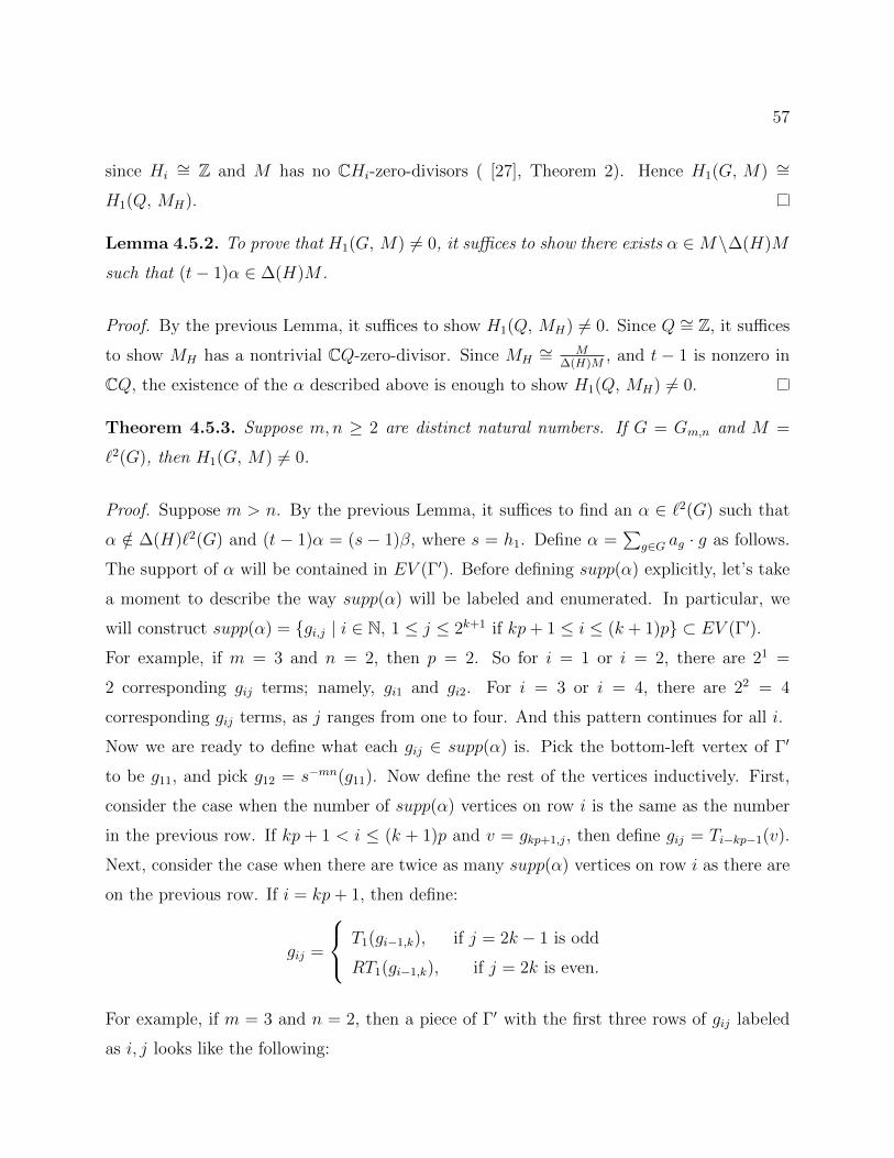
57

since Hi∼= Z and M has no CHi-zero-divisors ( [27], Theorem 2). Hence H1(G, M) ∼=

H1(Q, MH).

Lemma 4.5.2. To prove that H1(G, M) 6= 0, it suffices to show there exists α ∈M \∆(H)M

such that (t− 1)α ∈ ∆(H)M .

Proof. By the previous Lemma, it suffices to show H1(Q, MH) 6= 0. Since Q ∼= Z, it suffices

to show MH has a nontrivial CQ-zero-divisor. Since MH∼= M

∆(H)M, and t − 1 is nonzero in

CQ, the existence of the α described above is enough to show H1(Q, MH) 6= 0.

Theorem 4.5.3. Suppose m,n ≥ 2 are distinct natural numbers. If G = Gm,n and M =

`2(G), then H1(G, M) 6= 0.

Proof. Suppose m > n. By the previous Lemma, it suffices to find an α ∈ `2(G) such that

α /∈ ∆(H)`2(G) and (t − 1)α = (s − 1)β, where s = h1. Define α =∑

g∈G ag · g as follows.

The support of α will be contained in EV (Γ′). Before defining supp(α) explicitly, let’s take

a moment to describe the way supp(α) will be labeled and enumerated. In particular, we

will construct supp(α) = gi,j | i ∈ N, 1 ≤ j ≤ 2k+1 if kp+ 1 ≤ i ≤ (k + 1)p ⊂ EV (Γ′).

For example, if m = 3 and n = 2, then p = 2. So for i = 1 or i = 2, there are 21 =

2 corresponding gij terms; namely, gi1 and gi2. For i = 3 or i = 4, there are 22 = 4

corresponding gij terms, as j ranges from one to four. And this pattern continues for all i.

Now we are ready to define what each gij ∈ supp(α) is. Pick the bottom-left vertex of Γ′

to be g11, and pick g12 = s−mn(g11). Now define the rest of the vertices inductively. First,

consider the case when the number of supp(α) vertices on row i is the same as the number

in the previous row. If kp + 1 < i ≤ (k + 1)p and v = gkp+1,j, then define gij = Ti−kp−1(v).

Next, consider the case when there are twice as many supp(α) vertices on row i as there are

on the previous row. If i = kp+ 1, then define:

gij =

T1(gi−1,k), if j = 2k − 1 is odd

RT1(gi−1,k), if j = 2k is even.

For example, if m = 3 and n = 2, then a piece of Γ′ with the first three rows of gij labeled

as i, j looks like the following:

58

Now each group element g = gij in supp(α) needs to be assigned a nonzero complex number

ag = aij. If row i has 2k vertices in supp(α), then define:

aij =

2−k, 1 ≤ j ≤ 2k−1

−2−k, 2k−1 + 1 ≤ j ≤ 2k.

It follows that α is in `2(G):

∑i,j

|aij|2 =∞∑i=1

p · 2i ·(

1

2i

)2

<∞.

Now suppose that (t−1)α = (s−1)β. For precisely the same reasoning as in the G = B(1, n)

case, if β =∑g∈G

bg · g, then:

bg =∞∑k=0

(as−kg − at−1s−kg

).

Using the definition of α, we would like to show that β is in `2(G). First, consider the

β-coefficients from the rows of Γ′ for which the number of vertices in supp(α) is the same as

the row beneath it; let X be the set of all such vertices. Let row i be such a row. For all

relevant j-values, consider all vertices between gij and tgi−1,j, including the right endpoint

but not the left endpoint; there are at most b of them. And for each of these vertices v, the

largest that |bv| can be is 2−(k−1), for k such that kp+ 1 < i ≤ (k+ 1)p. All other bg on this

row are zero. Therefore: ∑g∈X

|bg|2 ≤ p∞∑k=1

b · 2k ·(

1

2k−1

)2

<∞.

59

Next, consider the β-coefficients for rows of Γ′ for which there are twice as many α-terms

as the row beneath it; let Y be the set of all such vertices. Suppose row i is such a row.

For all relevant odd j-values, consider all vertices between gij, gi,j+1 and tgi−1, j+12

, including

the right endpoint but not the left endpoint; there are at most b of them. For each of these

vertices v, the largest that |bv| can be is 2−(i−1). All other bg on this row are zero. Hence:∑g∈Y

|bg|2 ≤∞∑k=1

b · 2k ·(

1

2k−1

)2

<∞.

All other β-coefficients are zero.

It now only remains to show that α /∈ ∆(H)`2(G). Suppose α ∈ ∆(H)`2(G). Then there

exists q ∈ N such that α ∈ ∆(Hq)`2(G). This implies that there exists γ ∈ `2(G) such that

α = (hq − 1)γ. Define σ = hq. If γ =∑g∈G

cg · g, then:

cg = −∞∑k=0

aσ−kg.

If g = gij, then define cij = cg. Since there exists N ∈ N such that σN = s, it follows that

cij = −∞∑k=0

as−kg. Therefore, if i = kp + 1 and j = 2k−1 + 1 for any natural number k, then

cij = 12. Hence, γ is not in `2(G); a contradiction. Thus α /∈ ∆(H)`2(G).

If m < n, then build the subgraph Γ′ downward in the Cayley graph instead of upward. More

precisely, replace every “t” with “t−1” in the definition of Γ′. This will lead to analogous

definitions of T and p. After these alterations, the rest of the argument is the same as in the

case m > n.

Corollary 4.5.4. Suppose m,n ≥ 2 are distinct natural numbers. If G = Gm,n, then N (G)

is not flat over CG.

The theorem above applies to the module M = `p(G) with p = 2. However, the proof can

be easily modified to work for any p-values such that 1 < p ∈ R.

Theorem 4.5.5. Suppose m,n ≥ 2 are distinct natural numbers. If G = Gm,n and p > 1,

then `2(G) is not flat over CG.

Chapter 5

Elementary Amenable Groups

5.1 Introduction

Conjecture 1.1.1(A) was proved in Chapter 3. Conjecture 1.1.1(B) is still open in its most

general form, but this chapter will prove it for certain classes of groups. In particular, we

will show that the conjecture is true for the class of torsion-free elementary amenable groups.

Once that result has been proved, we can then show the conjecture to be true for the class of

elementary amenable groups which do not have infinite locally finite subgroups. The reason

this conjecture is more approachable for elementary amenable groups than it is in general

is the existence of an inductive definition of the class of elementary amenable groups. So

the main theorems of this chapter will be proved by induction. The results in this chapter

rely heavily upon three special cases which have already been considered: G = Z ⊕ Z,

G = B(1, n), and G = Gm,n. The fact that Conjecture 1.1.1(B) is true for these special cases

is foundational to the proofs for the larger classes of groups.

60

61

5.2 Elementary Amenable Groups

All of the groups in this chapter are elementary amenable groups. This class of groups is

defined as follows.

Definition 5.2.1. The class of elementary amenable groups EA is the smallest subclass of

the class of all groups which satisfies the following conditions:

1. EA contains all finite groups and all abelian groups,

2. if G ∈ EA and H ∼= G, then H ∈ EA,

3. EA is closed under the operations of taking subgroups, forming quotients, and forming

extensions, and

4. EA is closed under directed unions.

The class EA is contained in the class of all amenable groups ( [37], Propositions 0.15 and

0.16). However, these classes are not the same. For instance, Grigorchuk has constructed a

finitely presented group which is amenable but not elementary amenable [15].

The most important description of the class EA for our purposes is the inductive definition

given in Section 3 of [26]. First, we need to establish some notation. For two classes of groups

X and Y , say that a group G ∈ (LX )Y if G has a normal subgroup H such that H is locally

in X and G/H ∈ Y . Let B denote the class of all finitely generated abelian-by-finite groups.

For each ordinal α, define Xα inductively as follows:

X0 = 1,X1 = B,

Xα = (LXα−1)B if α is a successor ordinal, and

Xα =⋃β<α

Xβ, if α is a limit ordinal.

With this notation, the class of elementary amenable groups can be built by combining each

of these classes; EA =⋃α≥0

Xα.

62

The next theorem about the structure of elementary amenable groups should give an

indication about why the groups B(1, n) and Gm,n in particular are so important ( [14],

Theorem 5).

Theorem 5.2.2. Let G be an elementary amenable group of cohomological dimension ≤ 2.

1. Suppose that G is finitely generated. Then G possesses a presentation of the form

〈x, y | yxy−1 = xn〉.

2. Suppose that G is countable but not finitely generated. Then G is a non-cyclic subgroup

of the additive group Q.

5.3 Hirsch Length

Every elementary amenable group has a “Hirsch length” associated to it. This concept was

originally developed for polycyclic groups, which are a particular kind of solvable group.

Definition 5.3.1. A group G is said to be polycyclic if it has a subnormal series

1 = G0 / G1 / · · · / Gn−1 / Gn = G,

such that Gi+1/Gi is cyclic for each i = 0, 1, . . . , n − 1. A subnormal series of this form is

called a polycyclic series. The Hirsch length of a polycyclic group G, denoted h(G), is the

number of infinite factors in a polycyclic series of G.

The class of all polycyclic groups is a subclass of the class of all solvable groups, which in

turn is a subclass of EA. Using the inductive definition of EA above, the notion of Hirsch

length may be extended to make sense for all elementary amenable groups. If G ∈ X1, then

there exists an normal abelian subgroup A such that [G : A] < ∞. Let h(G) = rank(A).

Now suppose h(G) is defined for all groups in Xα. If G ∈ LXα, then define:

h(G) = sup h(G) | F ≤ G and F ∈ Xα.

If G ∈ Xα+1, then there exists a normal subgroup K / G with K ∈ LXα and G/K ∈ X1.

Define h(G) = h(K) + h(G/K).

63

There are a few facts about Hirsch length that will be utilized, such as the properties in

the next theorem ( [19], Theorem 1):

Theorem 5.3.2. Let G be an elementary amenable group. Then:

1. Hirsch length h(G) is well-defined.

2. If H ≤ G, then h(H) ≤ h(G).

3. Furthermore, h(G) = lubh(F ) | F is a finitely generated subgroup of G.

4. If H is a normal subgroup of G, then h(G) = h(H) + h(G/H).

The only elementary amenable groups that are torsion are the locally finite ones, and these

are the only groups in EA with trivial Hirsch length. More generally ( [19], p. 164):

Theorem 5.3.3. If G is an elementary amenable group and H is a locally finite normal

subgroup, then h(G/H) = h(G).

As a result of Lemma 2 in [19], there is the following bound on h(G).

Theorem 5.3.4. Hirsch length is bounded above by the rational cohomological dimension.

Groups of small Hirsch length have the following classification ( [19], Theorem 2):

Theorem 5.3.5. Let G be elementary amenable and let T be its maximal locally finite normal

subgroup. Then:

1. If h(G) <∞, then G ∈ LXh(G)+1.

2. If h(G) < 3, then G/T is solvable of derived length at most 5.

3. If h(G) = 1 or 2 and G is finitely generated, then G/T is virtually torsion-free.

64

5.4 Torsion-Free Elementary Amenable Groups

In this section we use the inductive definition of EA to prove Conjecture 1.1.1 for all torsion-

free elementary amenable groups.

Lemma 5.4.1. Let G be an additive subgroup of Q, and let ϕ ∈ Aut(G). Then ϕ(x) = rx

for some r ∈ Q.

Proof. Let Xn = k ∈ Z≥0 | kn∈ G, and let pn = min(Xn). Then Xn = kpn | k ∈ Z≥0.

Suppose ϕ(pnn

) = rn(pnn

). Then since ϕ is additive, ϕ(x) = rnx for all x ∈ G such that

x = kpnn

. Now note that every nonempty Xn intersects nontrivially with X1. Hence rn = r1

for all n, and so we may choose r = r1.

Lemma 5.4.2. Let G be a group with a normal subgroup H such that H is an additive

subgroup of the rational numbers, and G/H ∼= Z. Then G has a subgroup isomorphic to

Gp,q = Z[ 1pq

] o Z.

Proof. Let x ∈ G \H, and define f ∈ Aut(H) by f(h) = xhx−1. Since H is isomorphic to a

subgroup of Q that includes 1, we can assume that 1 ∈ H. By the Lemma above, f(y) = ry

for some r ∈ Q. Suppose r can be written as the reduced fraction pq. Then f i(1) = pi

qi∈ H

for all i ∈ Z. Hence api

qi+ b q

i

pi= ap2i+bq2i

piqi∈ H, for all a, b, i ∈ Z. Since gcd(p, q) = 1, we can

choose a, b such that 1piqi∈ H for all i ∈ Z. This implies that Z[ 1

pq] ≤ H; call this subgroup

K. Consider the following subgroup of G: A = 〈K, x〉. Then K is normal in A with quotient

isomorphic to Z, and the conjugation of x on K is equivalent to the homomorphism f above.

That is, A ∼= Gp,q.

The next theorem is the main theorem of this section. For any group G, let M(G) denote

either N (G) or `p(G) for any 1 < p ∈ R.

Theorem 5.4.3. Suppose G is a torsion-free elementary amenable group. If M(G) is flat

over CG, then G is locally cyclic.

65

Proof. First note that since every virtually cyclic group is either finite, finite-by-(infinite

cyclic), or finite-by-(infinite dihedral) and since we are only considering torsion-free groups,

we can use the terms “virtually cyclic” and “cyclic” interchangeably (see 7.1.7).

Recall the inductive definition of the class of elementary amenable groups. Let X0 = 1and let X1 be the class of finitely generated virtually abelian groups. If Xα has been defined

for some ordinal α let Xα+1 = (LXα)X1. If Xα has been defined for all ordinals α less than

some limit ordinal β let Xβ =⋃Xα. Then EA =

⋃Xα. The result will be proved by

induction on α.

Base Case: Consider G ∈ X1; suppose G is finitely generated virtually abelian. Then there

exists H ≤ G such that H is abelian and [G : H] <∞. Note that H cannot contain Z×Z as

a subgroup by the assumption thatM(G) is flat over CG. Hence H ∼= Z (note: a subgroup

of finite index of a finitely generated group is necessarily finitely generated). Hence G is

virtually cyclic.

Induction Hypothesis: Suppose the result is true for all groups in Xα.

Induction Step: We wish to show the result is true for all groups in Xα+1. If G ∈ Xα+1, then

there exists a normal subgroup H ∈ LXα such that G/H ∈ X1. SinceM(G) is flat over CG,

it must be the case that M(H) is flat over CH (see 2.8.1). By the induction hypothesis, H

is locally cyclic.

Case 1: Suppose G/H is finite. Since H is locally virtually cyclic, it follows that G is locally

virtually cyclic (see 7.1.3).

Case 2: Suppose Z ≤ G/H. Suppose x ∈ G is such that x generates the copy of Z in G/H,

and consider the subgroup G = 〈H, x〉. Then H is normal in G and G/H ∼= Z. It follows

that the Hirsch length is h(G) = h(H) + h(G/H) = 2 (see 5.3.2). By a theorem of Hillman,

it follows that G is solvable (see 5.3.5). The lowest nontrivial member of the derived series

for G is a torsion-free abelian normal subgroup K of G. Since M(G) is flat over CG, this

K cannot have Z × Z as a subgroup. Hence, K ∼= Z or K is a subgroup of Q which is not

finitely generated. Suppose K ∼= Z. Now pick g ∈ G \K and consider G′ = 〈K, g〉. This is a

finitely generated elementary amenable group of cohomological dimension 2. By a theorem

of Kropholler, Linnell, and Luck, it follows that G′ ∼= Z[ 1n] o Z for some n ∈ N (see 5.2.2).

Now suppose K is isomorphic to an additive subgroup of the rational numbers Q. In this

66

case still, K is normal in G′ and G′/K ∼= Z. And by the previous lemma, G′ ∼= Gm,n for

some natural numbers m and n. The result now follows.

5.5 Elementary Amenable Groups With Torsion

While the conjecture is still open for the full class of EA, we can do a little better than the

previous section. Again, for any group G, let M(G) denote either N (G) or `p(G) for any

1 < p ∈ R.

Theorem 5.5.1. Let G be an elementary amenable group with no infinite locally finite

normal subgroups. If M(G) is flat over CG, then G is locally virtually cyclic.

Proof. Just as in the torsion-free case, this will be a proof by induction.

Base Case: Consider G ∈ X1; suppose G is finitely generated virtually abelian. Then there

exists H ≤ G such that H is abelian and [G : H] <∞. Note that H cannot contain Z× Z

as a subgroup by the assumption that M(G) is flat over CG. Hence H is virtually Z or

finite (note: a subgroup of finite index of a finitely generated group is necessarily finitely

generated). Therefore, G is virtually cyclic.

Induction Hypothesis: Suppose the result is true for all groups in Xα.

Induction Step: We wish to show the result is true for all groups in Xα+1. If G ∈ Xα+1, then

there exists normal subgroup H ∈ LXα such that G/H ∈ X1. Since M(G) is flat over CG,

it must be the case that M(H) is flat over CH. By the induction hypothesis, H is locally

virtually cyclic.

Case 1: Suppose G/H is finite. Since H is locally virtually cyclic, it follows from a theorem

in the appendix (7.1.3) that G is locally virtually cyclic.

Case 2: Suppose Zn ≤ G/H for the largest possible n ∈ N. Suppose x1, x2, . . . , xn ∈ G

are such that x1, x2, . . . , xn generates the copy of Zn in G/H, and consider the subgroup

G1 = 〈H, x1〉. Then H is normal in G1 and G1/H ∼= Z. Since H is locally virtually cyclic,

it follows that h(H) = 1 and h(G1) = h(H) + h(G1/H) = 2. Let B1 be an arbitrary finitely

generated subgroup of G1. Then h(B1) ≤ h(G1) = 2. By a theorem of Hillman (5.3.5), there

is a locally finite normal subgroup T1 of B1 such that B1/T1 is virtually torsion-free. By

67

assumption, T1 must be finite. Let K1 be atorsion-free subgroup of B1/T1 of finite index.

Since M(G) is flat over CG, it follows that M(B1) is flat over CB1 (see 2.8.1), and hence

M(B1/T1) is flat over C[B1/T1] (see 2.8.8), and so M(K1) is flat over CK1 (see 2.8.1). By

the torsion-free case, K1 must be locally virtually cyclic. Then both B1/T1 and B1 are

locally virtually cyclic (see 7.1.3 and 7.1.9). Since B1 is finitely generated, it follows that B1

is virtually cyclic. Since B1 was an arbitrary finitely generated subgroup of G1, it follows

that G1 is locally virtually cyclic. Consider G2 = 〈G1, x2〉. Then G1 is normal in G2 and

G2/G1∼= Z. By repeating the steps above, for any finitely generated subgroup B2 of G2,

there is a finite normal subgroup T2 of B2 and a torsion-free subgroup K2 of B2/T2 of finite

index. And, for the same reasoning as above, it must be the case that G2 is locally virtually

cyclic. Then consider G3 = 〈G2, x3〉. We can continue this process until we have used up

all of x1, x2, . . . , xn. Since Gn is locally virtually cyclic, it must be the case that G is locally

virtually cyclic.

Chapter 6

Special Cases and Future Steps

6.1 Introduction

Not all elementary amenable groups were covered in Chapter 5. In particular, groups with

infinite locally finite subgroups were not allowed. Conjecture 1.1.1 is still open for most of

these groups. However, a few special cases will be covered in this chapter. Consider a group

G with infinite locally finite normal subgroup H and quotient Q = G/H. First, we will

consider the case when Q = Z, such as the Lamplighter Group. In general, the proof used

for such groups cannot be extended to the case when the quotient is more complicated, such

as Q = Z ⊕ Z. However, if H is assumed to be abelian, then we can show the result to be

true for more complicated quotients.

6.2 The Lamplighter Group

Linnell, Schick, and Luck proved that Conjecture 1.1.1 is true for the “Lamplighter Group”

[30]. That argument will be discussed in this section, and it will be generalized for a larger

class of groups. First, let’s define what the Lamplighter Group is. It is defined using a

wreath product, which is a semidirect product.

68

69

Definition 6.2.1. Let A,H be groups, and let Ω be a set such thatH acts on Ω. LetK be the

direct sum⊕ω∈ΩAω. ThenH acts onK: h·(aω) = (ah−1ω). Then the restricted wreath product,

denoted A oH, is the semidirect product K oH. The wreath product is regular if Ω = H.

The Lamplighter Group is the regular restricted wreath product Z2 o Z. So it has a normal

subgroup N ∼= ⊕ZZ2 such that G/N ∼= Z. We will consider all finitely generated groups

(including the Lamplighter Group) with an infinite locally finite normal subgroup H such

that H is countably generated and G/H ∼= Z.

The proof for this class of groups will require some basic knowledge about a group’s

cohomological and homological dimensions.

Definition 6.2.2. The R-module C has flat dimension n if there exists a flat resolution of

length n: 0 → Qn → Qn−1 → · · · → Q0 → C → 0. And C has projective dimension n if

there exists a projective resolution of length n: 0→ Pn → Pn−1 → · · · → P0 → C → 0. The

cohomological dimension of G over R is defined to be the projective dimension of R as an

RG-module, denoted cdRG. The homological dimension of the group G over the ring R is

defined to be the flat dimension of R as an RG-module

In particular, the following facts about cdRG will be necessary (see p. 70, p. 53, Proposition

4.12 and Theorem 4.7 in [5]).

Lemma 6.2.3. Let G be a group.

1. cdRG = 0 if and only if G is a finite group with no R-torsion (i.e., |G| is a unit in R).

2. If G = lim−→Gα for a direct system of groups Gα | α ∈ I such that I is countable, then

cdRG ≤ sup cdRGα+ 1.

3. If H is a normal subgroup, then cdRG ≤ cdRH + cdR(G/H).

4. Suppose Pn−1 → Pn−2 → · · · → P0 → C → 0 is part of a projective resolution of C.

Then cdCG = n if and only if K = ker (Pn−1 → Pn−2) is projective.

70

And the following analogous facts about hdRG will also be used (see p. 70, p. 52, Proposition

4.12 and Theorem 4.7 in [5]).

Lemma 6.2.4. Let G be a group.

1. hdRG = 0 if and only if G is a locally finite group with no R-torsion.

2. If G = lim−→Gα for a direct system of groups Gα | α ∈ I, then hdRG ≤ sup hdRGα.

3. If H is a normal subgroup, then hdRG ≤ hdRH + hdR(G/H).

4. hdCG = n if and only if TorCGn+1(B, C) = 0 for all CG-modules B.

The structure of “almost finitely presented groups” and HNN-extensions will also play a role.

Definition 6.2.5. Let k be a commutative ring with unit. A group G is called almost finitely

presented over k if there is a presentation G = F/R, such that F is a finitely generated free

group and the tensor product R/[R,R]⊗Z k is finitely generated as a kG-module.

Definition 6.2.6. Let G be a group with presentation G = 〈S|R〉, let H,K ≤ G, and

suppose α : H → K is an isomorphism. Let t denote a new symbol. Then the HNN-extension

is defined to be G∗α = 〈S, t | R, tht−1 = α(h),∀h ∈ H〉, and t is called the stable letter.

The following two facts regarding HNN-extensions will be necessary (see Britton’s Lemma

on p. 181 of [32], and p. 259 in [6]).

Lemma 6.2.7. 1. In the notation above for HNN-extensions, if H 6= G and K 6= G, then

the HNN-extension G∗α contains a subgroup isomorphic to Z ∗ Z.

2. Let G be a group containing a normal subgroup N with infinite cyclic quotient G/N ,

and let t ∈ G be an element with gp(t, N) = G. If G is almost finitely presented over

some ring k, then G is an HNN-group with stable letter t such that both base group and

associated subgroups are finitely generated and contained in N .

71

An interesting feature of this section, in contrast to the previous sections, is that a result

for N (G) will be reached by way of a result for U(G). In cases such as this, it can be useful

to have an abundance of invertible elements around. For a group G, let D(G) denote the

division closure of CG in U(G). If k is a field and g ∈ G has infinite order, then 1 − g is a

non-zero-divisor in kG, and in the case k = C we also have that 1− g is invertible in D(G)

(see [30], p. 2). In particular, the resulting lemma will be utilized.

Lemma 6.2.8. If G contains an element of infinite order, then U(G)⊗CG C = 0.

Proof. If g ∈ G has infinite order, then we know that 1−g is invertible in U(G). This means

for an element of the form x ⊗ y of the tensor product, 1 − g can be factored out of x and

brought across the tensor, at which point it acts on y, making it 0.

The final necessary lemma can be found on p. 3 of [30].

Lemma 6.2.9. Let R be a subring of the ring S and let P be a projective R-module. If

P ⊗R S is finitely generated as an S-module, then P is finitely generated.

Now we are ready to prove the main result of this section.

Theorem 6.2.10. Suppose G is a finitely generated group with an infinite locally finite

normal subgroup H such that H is countably generated and G/H ∼= Z. Then N (G) is not

flat over CG.

Proof. First note that since G contains an element of infinite order that U(G) ⊗CG C = 0

(see 6.2.8). Since G is finitely generated, we have the following two exact sequences of

CG-modules:

0→ I → CG→ C→ 0

0→ P → CGd → I → 0

where I represents the augmentation ideal, and d is the minimum number of group elements

needed to generate G. Now suppose that TorCG1 (U(G),C) = 0 (this assumption will lead

72

to a contradiction). In this case, applying the functor U(G) ⊗CG − to the first piece of the

resolution yields the exact sequence:

0→ U(G)⊗CG I → U(G)⊗CG CG→ U(G)⊗CG C = 0.

It follows that U(G)⊗CG I ∼= U(G)⊗CGCG ∼= U(G). Note that hdCH = 0 by 6.2.4(1). Since

hdC(Z) = 1, it follows that hdC(G) = 1 (see 6.2.4(3)). By 6.2.4(4), 0 = TorCG2 (U(G),C) =

TorCG1 (U(G), I), and thus we can apply U(G)⊗CG− to the second piece of the resolution to

obtain the exact sequence:

0→ U(G)⊗CG P → U(G)⊗CG CGd → U(G)⊗CG I → 0

which can be rewritten as:

0→ U(G)⊗CG P → U(G)d → U(G)→ 0.

This implies that U(G) ⊗CG P is a finitely generated projective U(G)-module. But since

cdCH ≤ 1 (see 6.2.3(1) and 6.2.3(2)), we know that cdC(G) ≤ 2 (see 6.2.3(3)). Thus P must

be a projective CG-module (see 6.2.3(4)). Thus P must be a finitely generated projective

CG-module (see 6.2.9). However, if G ∼= F/R where F is a free group on d generators, then

we know that P ∼= R/[R,R] ⊗ C [20]. By definition, G is almost finitely presented over C.

Thus G is an HNN-extension (see 6.2.7(1)) and must therefore have a subgroup isomorphic

to Z ∗ Z (see 6.2.7(2)). This is a contradiction. Hence TorCG1 (U(G),C) 6= 0, and so U(G) is

not flat over CG. It now follows that N (G) is not flat over CG (see 2.8.17).

6.3 Other Groups

Say that a group G has property (P1) if it is finitely generated and there exists an infinite

locally finite normal subgroup H, which is countably generated, such that G/H ∼= Z. And

say that a group G has property (P2) if there exists a finite normal subgroup H such that

G/H ∼= Z× Z. Say that a group has property (P3) if there exists a finite normal subgroup

H such that G/H ∼= Z[ 1n] o Z.

73

Theorem 6.3.1. Let G be a group, and let H be an abelian infinite locally finite normal

subgroup, which is countably generated, such that G/H ∼= Z × Z. Then G either has a

subgroup with property (P1) or has a subgroup with property (P2). Hence, Conjecture 1.1.1

holds for G.

Proof. Let x, y ∈ G be such that G/H = 〈x, y〉. Let a = [x, y]. Since a = 1 in G/H it

follows that a ∈ H. Let X = axiyj | i, j ∈ Z, B = 〈X〉, and C = 〈B, x, y〉. Assume that G

does not have a subgroup with property (P1). Then it suffices to prove the following three

claims:

1. B is finite,

2. B is normal in C, and

3. C/B ∼= Z× Z.

Claim 1: Define X1 = axi | i ∈ Z. If we define K = 〈a, x〉 and assume X1 is infinite then

H ∩ K will be infinite. And hence H ∩ K is infinite locally finite and normal in K such

that K/(H ∩ K) ∼= 〈x〉 ∼= Z. In other words, K satisfies property (P1). Therefore X1 is

finite. For every b ∈ X1, define X2(b) = byi | i ∈ Z. Similar to the previous argument, if

any X2(b) is infinite then 〈b, y〉 will have property (P1). Therefore X2(b) is finite for every

b ∈ X1. It follows that X =⋃b∈X1

X2(b) is finite. Since H is locally finite, B must be finite.

Claim 2: Note that if h ∈ H and b ∈ B then bh = b, since H is abelian. Hence for all i, j ∈ Z

there exists h ∈ H such that(ax

iyj)x

= ahxi+1yj = ax

i+1yj ∈ B. It follows that B is normal

in C.

Claim 3: This follows from the fact that a ∈ B (and nothing else is in B that can’t be built

with conjugates of a).

Theorem 6.3.2. Let G be a group, and let H be an abelian infinite locally finite normal

subgroup, which is countably generated, such that G/H ∼= Z[ 1n] o Z. Then G either has a

subgroup with property (P1) or has a subgroup with property (P3). Hence, Conjecture 1.1.1

holds for G.

74

Proof. Let x, y ∈ G generate G/H such that yxy−1x−n = 1 in G/H. Define a = yxy−1x−n ∈H, and let A = 〈a〉. Let X = ayixjyk | i, j, k ∈ Z. Define B = 〈X〉 and C = 〈B, x, y〉.Assume G has no subgroups with property (P1). Then it suffices to prove the following three

claims:

1. B is finite,

2. B is normal in C, and

3. C/B ∼= Z[ 1n] o Z.

Claim 1: Let X1 = ayi | i ∈ Z. If X1 is infinite, then the subgroup 〈a, y〉 has property

(P1). Hence X1 must be finite. For each b ∈ X1, define X2(b) = bxi | i ∈ Z. If any X2(b)

is infinite then 〈b, x〉 has property (P1). Hence X2(b) must be finite for every b ∈ X1. If

c ∈ X2(b) for some b ∈ X1, then define X3(c) = cyi | i ∈ Z. Then each such X3(c) must

also be finite. It follows that X =⋃b∈X1

⋃c∈X2(b)

X3(c)

is finite. Since H is locally finite, B

must be finite.

Claim 2: The key fact here is that each element of G/H can be represented by an element

of the form yixjyk [8]. Note also that bh = b for every b ∈ B and h ∈ H, since H is

abelian. In particular, for every i, j, k ∈ Z there exist p, q, r ∈ Z and h ∈ H such that(ay

ixjyj)x

= ahypxqyr = ay

pxqyr ∈ B. Therefore B is normal in C.

Claim 3: This follows from the fact that a ∈ B (and nothing else is in B that can’t be built

with conjugates of a).

6.4 Future Steps

So far, Conjecture (B) has been proved for the class of elementary amenable groups without

infinite locally finite subgroups. It is not yet clear how to extend this result to the class of

all elementary amenable groups. In order to make that generalization, it will probably be

75

necessary to prove a version of 2.8.8 in which H is allowed to be infinite locally finite. It is

even less clear how to prove this result for the class of amenable groups (including groups

which are not elementary amenable), however that may be an interesting question for future

study. As for the class of non-amenable groups, the result is known for groups that have

nonabelian free subgroups, but the general case is still open. Since such groups are far from

being in the conjectured class of acceptable groups (locally virtually cyclic groups), proving

the conjecture for the class of non-amenable groups could very well be doable.

Other variations of Conjecture (B) could also be studied. For instance, in this paper, many

of the results for the moduleN (G) were also shown to be true for the modules `p(G). Perhaps

the CG-module C∗(G), the group C∗-algebra of G, could be similarly explored. Some basic

results were obtained in section 2.7 concerning the groups G = Z and G = Z⊕Z, but much

of the work in this paper has not yet been shown to hold for this module. Another variation

of the work in this paper would be to study group cohomology rather than group homology.

Once again, there are some elementary results in sections 2.5 and 2.6, but perhaps much

more could be said. One could also consider module-theoretic properties of N (G) other than

flatness. Is N (G) a free module only when G is finite? Is N (G) a projective module only

when G is finite? For which groups, if any, is N (G) an injective module? What about U(G)?

Conjecture (A) is still open as well. Proving it in its full generality would be a big

accomplishment, but perhaps there are weaker versions of it that could be proved more

easily. Or it might be worthwhile to attempt to calculate some L2-invariants for groups

which are non-amenable to see if they vanish or not. However, since this conjecture is known

for groups with nonabelian free subgroups, that limits the choices of groups that would be

interesting in this context. This conjecture could also be studied with regard to Thompson’s

group. Since it is unknown whether Thompson’s group is amenable or not, calculating any of

the dimensions in Conjecture (A) would be of interest. It is already known that the L2-Betti

numbers of Thompson’s group vanish (Corollary 6.8 in [10]).

Chapter 7

Appendix

7.1 Locally Virtually Cyclic Groups

There are several facts about virtually cyclic groups that are utilized in the proofs by induc-

tion in Sections 5.4 and 5.5. Here are those facts, with lemmas interspersed as necessary.

Lemma 7.1.1. If G is a finitely generated group and H is a subgroup of finite index, then

H is finitely generated.

Proof. This is a consequence of “Schreier’s formula.” See Proposition 12.1 in [32].

Lemma 7.1.2. If H and K are subgroups of a group G, then [H : H ∩K] ≤ [G : K].

Proof. See Proposition 4.8 in [21].

Theorem 7.1.3. Suppose H is a locally virtually cyclic subgroup of G of finite index. Then

G is locally virtually cyclic.

Proof. Let G1 ≤ G be a finitely generated subgroup. We wish to show that G1 is virtually

cyclic. Let H1 = H ∩ G1 ≤ G1. Then H1 ≤ H implies H1 is locally virtually cyclic. And

[G1 : H1] = [G1 : H ∩G1] ≤ [G : H] <∞. Since G1 is finitely generated and [G1 : H1] <∞,

76

77

it follows that H1 is finitely generated. Therefore H1 is virtually cyclic. Since H1 is virtually

cyclic and [G1 : H1] <∞, it follows that G1 is virtually cyclic.

Theorem 7.1.4. If a group is finite-by-cyclic, then it is virtually cyclic.

Proof. The finite-by-finite case is obvious, so suppose the quotient is infinite cyclic. Let

H = 〈h1, h2, . . . , hn〉 be a finite normal subgroup such that Q = G/H ∼= Z. Suppose x ∈ Gis such that x generates Q. Consider K = 〈x〉. Since K is cyclic, it suffices to show that

[G : K] <∞. Note that G has the following left cosets with respect to H:

H, xH, x2H, x3H . . .

Take one element from each of these cosets as follows:

h1, xh1, x2h1, x

3h1, . . .

Note that these elements form the right cosetKh1. Similarly, form the right cosetsKh2, Kh3, . . . , Khn.

Since the left cosets above with respect to H exhaust G, so must the right cosets with respect

to K. Clearly these right cosets are disjoint since the H cosets are disjoint and since:

xihj = xihm ⇒ hj = hm ⇒ j = m

Lemma 7.1.5. If H is a subgroup of G, then the “normal core” of H satisfies the following

inequality: [G : Core(H)] ≤ [G : H]!.

Proof. See Exercise 20 on page 48 in [17].

Theorem 7.1.6. If a group G is infinite virtually cyclic, then there exists a normal infinite

cyclic subgroup of finite index.

Proof. Since G is infinite virtually cyclic, there exists an infinite cyclic subgroup H of finite

index. Let K = Core(H). Since G is infinite and [G : K] ≤ [G : H]! < ∞, it follows that

K must be nontrivial. Since H is infinite cyclic and K ≤ H, K must also be infinite cyclic.

The result now follows.

78

The following theorem can be found in Lemma 11.4 of [16].

Theorem 7.1.7. Groups of the following three types are virtually cyclic. Moreover, every

virtually cyclic group is exactly one of these types:

1. finite

2. finite-by-(infinite cyclic)

3. finite-by-(infinite dihedral)

Theorem 7.1.8. Suppose H is a finite normal subgroup of G such that G/H is virtually

cyclic. Then G is virtually cyclic.

Proof. If G/H is finite, then G is finite and hence virtually cyclic. Suppose Q = G/H is

infinite. By Theorem 7.1.7, there exists a finite normal subgroup A of Q such that Q/A

is either infinite cyclic or infinite dihedral. By the Correspondence Theorem, there exists

a normal subgroup K of G, which contains H, such that A ∼= K/H. Since A and H are

finite, we know that K is finite also. By the Third Isomorphism Theorem, G/K ∼= Q/A,

which implies G/K is either infinite cyclic or infinite dihedral. Therefore, G is either finite-

by-(infinite cyclic) or finite-by-(infinite dihedral). By 7.1.7, G must be virtually cyclic.

Corollary 7.1.9. Suppose H is a finite normal subgroup of G such that G/H is locally

virtually cyclic. Then G is locally virtually cyclic.

Proof. Let K be an arbitrary finitely generated subgroup of G; it suffices to show K is

virtually cyclic. Consider K = 〈K,H〉, which is still finitely generated and H / K. Thus

K/H is a finitely generated subgroup of G/H, which implies K/H is virtually cyclic. By

the previous theorem, it follows that K is virtually cyclic, which implies that K is virtually

cyclic.

79

7.2 Left Modules vs. Right Modules

This paper has primarily sought out connections between the structure of groups and the

module-theoretic structure of N (G). In particular, the module-theoretic property that has

been featured is flatness. There are other module properties one could also explore, such as

freeness, projectivity, or injectivity. No conjectures have been made yet connecting properties

of G to these potential properties of N (G) (although, a reasonable guess is that N (G) is

free only if G is finite). However, if one wanted to study such questions, one practical matter

is this: is it possible for N (G) to have one of those properties as a left-module while not

having it as a right-module? This section provides that question with an answer of “no.”

First, consider the question of when N (G) is a free module. Recall that an R-module M

is called free if M is isomorphic to a direct sum of copies of R.

Theorem 7.2.1. If G is a group, then N (G) is free as a left CG-module if and only if N (G)

is free as a right CG-module.

Proof. Suppose N (G) is free as a left CG-module. Then there exists an isomorphism f :

CGα → N (G). Construct a map of right CG-modules f ′ : CGα → N (G) by f ′(x) = f(x∗)∗.

Then for any x ∈ CGα and any r ∈ CG we have:

f ′(x) · r = f(x∗)∗r = (r∗f(x∗))∗ = (f(r∗x∗))∗ = f ′(xr).

And for any x, y ∈ CG∗:

f ′(x+ y) = f(x∗ + y∗)∗ = f(x∗)∗ + f(y∗)∗ = f ′(x) + f ′(y).

Hence, f ′ is a right CG-homomorphism. Suppose f ′(x) = 0. Then f(x∗)∗ = 0, which implies

f(x∗) = 0. Since f is injective, this means x∗ = 0, and hence x = 0. Therefore f ′ is injective.

And since f is surjective, it clearly follows that f ′ is surjective too. Therefore, N (G) is free

as a right CG-module. Similarly, the converse is also true.

80

Now consider the property of projectivity. An R-module M is called projective if and only

if M is a summand of a free module. Another equivalent way to define projective modules

is with the existence of a “projective basis,” as described in the next lemma ( [40], Theorem

3.15).

Lemma 7.2.2. A left module A is projective if and only if there exist elements ak | k ∈K ⊂ A and R-maps fk : A→ R | k ∈ K such that

1. if x ∈ A, then almost all fk(x) = 0, and

2. if x ∈ A, then x =∑k∈K

fk(x)ak.

There is an analogous characterization of projective right modules.

Theorem 7.2.3. If G is a group, then N (G) is projective as a left CG-module if and only

if N (G) is projective as a right CG-module.

Proof. Suppose N (G) is projective as a left CG-module. Then there exists a projective basis

as described in the previous lemma. For all k ∈ K define f ′k(x) = fk(x∗)∗. These are right

CG-homomorphisms. We’d like to show, for any x, that f ′k(x) = 0 for almost all k. If

f ′k(x) = 0, then fk(x∗)∗ = 0, which means fk(x

∗) = 0. By property (1) in the lemma, this

must be true for almost all k ∈ K. Finally:

x∗ =(∑

fk(x)ak

)∗=∑

a∗k (fkx)∗ =∑

a∗kf′k(x∗).

Hence, property (2) of the lemma is satisfied for N (G) as a right module with respect to

the maps f ′k and the elements a∗k. Therefore N (G) is projective as a right CG-module.

Similarly, the converse is also true.

Finally, we will consider the property of injectivity. The most useful characterization of

injective modules will be the “Baer Criterion,” which can be found in Theorem 3.20 in [40]

and is listed below.

81

Lemma 7.2.4. A left R-module E is injective if and only if every map f : I → E, where I

is a left ideal of R, can be extended to R. There is an analogous definition for right modules.

Theorem 7.2.5. If G is a group, then N (G) is injective as a left CG-module if and only if

N (G) is injective as a right CG-module.

Proof. SupposeN (G) is injective as a left CG-module. Let I be a right ideal of CG generated

by ai, and let f : I → N (G) be a right CG-map. We wish to show that f can be

extended to all of CG. Consider the right ideal I ′ generated by a∗i and the left CG-map

f ′ : I ′ → N (G) defined by f ′(x) = f(x∗)∗. By the previous lemma, f ′ has an extension

f ′e : CG→ N (G). Now define a right CG-map fe : CG→ N (G) by fe(x) = f ′e(x∗)∗. Then I

claim that fe is an extension of f . Let a1r1 + · · ·+ anrn be an arbitrary element of I. Then:

fe(a1r1 + · · ·+ anrn) = f ′e(r∗1a∗1 + · · ·+ r∗na

∗n)∗ = f ′(r∗1a

∗1 + · · ·+ r∗na

∗n)∗ = f(a1r1 + · · ·+ anrn).

Therefore, N (G) is injective as a right CG-module. Similarly, the converse is also true.

Bibliography

[1] Frank W. Anderson and Kent R. Fuller. Rings and Categories of Modules. Springer-

Verlag, 1974.

[2] G. Baumslag and R. Strebel. Some finitely generated, infiinitely related metabelian

groups with trivial multiplicator. J. Algebra, 40:46–62, 1976.

[3] Gilbert Baumslag and Donald Solitar. Some two-generator one-relator non-Hopfian

groups. Bulletin of the American Mathematical Society, 68:199–201, 1962.

[4] R. Benedetti and C. Petronio. Lectures on Hyperbolic Geometry. Springer-Verlag, 1992.

[5] Robert Bieri. Homological Dimension of Discrete Groups. Mathematics Dept., Queen

Mary College, University of London, 2nd edition, 1981.

[6] Robert Bieri and Ralph Strebel. Almost finitely presented soluble groups. Commentarii

Mathematici Helvetici, 53:258–278, 1978.

[7] Kenneth S. Brown. Cohomology of Groups. Springer-Verlag, 1982.

[8] D.J. Collins. Baumslag-Solitar group. In Encyclopedia of Mathematics. Springer, 2001.

[9] Kenneth R. Davidson. C∗-algebras by Example. American Mathematical Society, 1996.

[10] Warren Dicks and Peter Linnell. L2-Betti numbers of one-relator groups. Math. Ann.,

337:855–874, 2007.

[11] David S. Dummit and Richard M. Foote. Abstract Algebra. John Wiley and Sons, Inc.,

2004.

82

83

[12] Ralph Fox. Free Differential Calculus I: Derivation in the Free Group Ring. Annals of

Mathematics, 57(3):547–560, 1953.

[13] Ralph Fox. Free Differential Calculus V: The Alexander Matrices Re-Examined. Annals

of Mathematics, 71(3):408–422, 1960.

[14] Dion Gildenhuys. Classification of soluble groups of cohomological dimension two. Math-

ematische Zeitschrift, 166:21–25, 1979.

[15] R.I. Grigorchuk. An example of a finitely presented amenable group that does not

belong to the class EG. Mat. Sb., 189(1):79–100, 1998.

[16] John Hempel. 3-Manifolds. American Mathematical Society, 2004.

[17] I.N. Herstein. Topics in Algebra. Blaisdell Pub. Co., 1964.

[18] E. Hewitt and K.A. Ross. Abstract Harmonic Analysis. Springer-Verlag, 1979.

[19] Jonathan Hillman. Elementary amenable groups and 4-manifolds of Euler characteristic

0. J. Austral. Math. Soc. Ser. A, 50(1):160–170, 1991.

[20] H. Hopf. Fundamentalgruppe und zweite bettische gruppe. Comment. Math. Helv.,

14(1):257–309, 1942.

[21] Thomas W. Hungerford. Algebra. Springer-Verlag, 1974.

[22] Adrian Ioana, Sorin Popa, and Stefaan Vaes. A class of superrigid group von Neumann

algebras. arXiv: 1007.1412v2, 2011.

[23] R. V. Kadison. Operator algebras - an overview. In The Legacy of John von Neumann,

pages 61–89. American Mathematical Society, 1990.

[24] A. A. Kirillov. Elements of the Theory of Representations. Springer-Verlag, 1972.

[25] Peter Kropholler, Peter Linnell, and Wolfgang Luck. Groups of small homological

dimension and the Atiyah conjecture. In Geometric and cohomological methods in group

theory, pages 272–277. Cambridge Univ. Press, 2009.

84

[26] P.H. Kropholler, P.A. Linnell, and J.A. Moody. Applications of a new K-theoretic

theorem to soluble group rings. Proc. Amer. Math. Soc., 104:675–684, 1998.

[27] Peter Linnell. Zero divisors and group von Neumann algebras. Pacific Journal of

Mathematics, 149(2), 1991.

[28] Peter Linnell. Division rings and group von Neumann algebras. Forum Mathematicum,

5:561–576, 1993.

[29] Peter Linnell. Analytic versions of the zero divisor conjecture. In Geometry and coho-

mology in group theory, pages 209–248. Cambridge University Press, 1998.

[30] Peter Linnell, Wolfgang Luck, and Thomas Schick. The Ore condition, affiliated opera-

tors, and the Lamplighter group. In High-dimensional manifold topology, pages 315–321.

World Sci. Publ., 2003.

[31] Wolfgang Luck. L2-Invariants: Theory and Applications to Geometry and K-Theory.

Springer-Verlag, 2002.

[32] Roger C. Lyndon and Paul E. Schupp. Combinatorial Group Theory. Springer-Verlag,

2001.

[33] George W. Mackey. The Theory of Unitary Group Representations. The University of

Chicago Press, 1976.

[34] Dusa McDuff. Uncountably many II1 factors. Annals of Mathematics, 90(2):372–377,

1969.

[35] A.Y. Ol’Shanskii and M.V. Sapir. Non-amenable finitely presented torion-by-cyclic

groups. Electron. Res. Announc. Amer. Math. Soc., 7:63–71, 2001. electronic.

[36] Narutaka Ozawa. Weakly exact von Neumann algebras. J. Math. Soc. Japan, 59(4):985–

991, 2007.

[37] A.L.T. Paterson. Amenability. American Mathematical Society, Providence, RI, 1988.

85

[38] Sorin Popa. Deformation and rigidity for group actions and von Neumann algebras. In

Proceedings of the International Congress of Mathematicians, pages 445–477, 2007.

[39] Michael Puls. Zero divisors and Lp(G). Proc. Amer. Math. Soc., 126(3):721–728, 1998.

[40] Joseph J. Rotman. An Introduction to Homological Algebra. Academic Press, 1979.

[41] Walter Rudin. Fourier Analysis on Groups. Interscience Publishers, 1962.

[42] Thomas Schick. Integrality of L2-Betti numbers. Mathematische Annalen, 317:727–750,

2000.

[43] John Stallings. Group theory and three-dimensional manifolds. In Yale Mathematical

Monographs. Yale University Press, 1971.

[44] B. Strenstrom. Rings of Quotients. Springer-Verlag, 1975.

[45] John von Neumann. Zur algebra der funktionaloperationen und theorie der normalen

operatoren. Math. Ann., 102(1):370–427, 1929.

[46] John von Neumann. On rings of operators. Annals of Mathematics, 37(1):116–129,

1936.

[47] Charles A. Weibel. Introduction to Homological Algebra. Cambridge University Press,

1994.