1

COMPARISONS INVOLVING TWO SAMPLE MEANS Testing Hypotheses Two types of hypotheses:

1. Ho: Null Hypothesis - hypothesis of no difference. § 21 µµ = or 021 =−µµ

2. HA: Alternate Hypothesis – hypothesis of difference.

§ 21 µµ ≠ or 021 ≠−µµ Two-tail vs. One-tail Tests

§ Two-tail tests have these types of hypotheses: Ho: 21 µµ = HA: 21 µµ ≠

§ Note the presence of the equal signs. § If you reject Ho: 21 µµ = , you don’t care which mean is greater. § 1µ can be either greater than or less than 2µ .

§ One-tail tests my have one of the following types of hypotheses:

Ho: 21 µµ ≥ Ho: 21 µµ ≤ HA: 21 µµ < HA: 21 µµ >

§ Note the presence of greater than or less than signs. § If you reject Ho:, you are being specific that 1µ can only be on one side

of 2µ .

t-Distribution 2/α 2/α α

Two-tail test One-tail test Size of the rejection region = 2/α Size of the rejection region =α

2

Types of Errors 1. Type I Error: To reject the null hypothesis when it is actually true. § The probability of committing a Type I Error is α . § The probability of committing a Type I Error can be reduced by the investigator

choosing a smaller α . § typical sizes of α are 0.05 and 0.01. § The probability of committing a Type I Error also can be expressed as a

percentage (i.e. α *100 %) § If α =0.05, The probability of committing a Type I Error is 5%. § If α =0.05, we are testing the hypothesis at the 95% level of confidence. 2. Type II Error: The failure to reject the null hypothesis when it is false.

§ The probability of committing a Type II Error is β . § β can be decreased by:

a. Increasing n (i.e. the number of observations per treatment). b. Decreasing s2.

§ Increase n § Choose a more appropriate experimental design § Improve experimental technique.

Power of the Test

§ Power of the test is equal to: 1- β . § Defined as the probability of accepting the alternate hypothesis when it is true. § We want the Power of the Test to be as large as possible.

Summary of Type I and Type II Errors True Situation

Decision Null hypothesis is true Null hypothesis if false

Reject the null hypothesis Type I Error No error

Fail to reject the null hypothesis No error Type II Error

3

Graphical Representation of σ and β Assume you have the hypothesis

Ho:µ=µ0 HA:µ=µ1

and we have two normal distributions, with mean equal to µ0 and µ1, respectively, and a variance for both of σ2. The following distributions can be drawn,

• Let the decision to reject H0 (i.e., accept HA) or fail to reject H0 be based on one

random observation.

• If the random observation is > C then we reject H0. • Paying attention only to the distribution assuming H0 is true, we can see that a

Type I Error was committed because the rejection region is “truly” part of the distribution.

• Thus, the probability of committing a Type I Error = α, which is shown

graphically, is solely dependent on the null hypothesis. • If the random observation is < C, then we fail to reject H0.

• Paying attention to the distribution assuming HA is true, we can see that a Type II

Error was committed because we wrongly failed to reject H0 when we should have.

• Thus, the probability of committing a Type II Error = β, which is shown

graphically, is dependent on the null and alternate hypotheses.

4

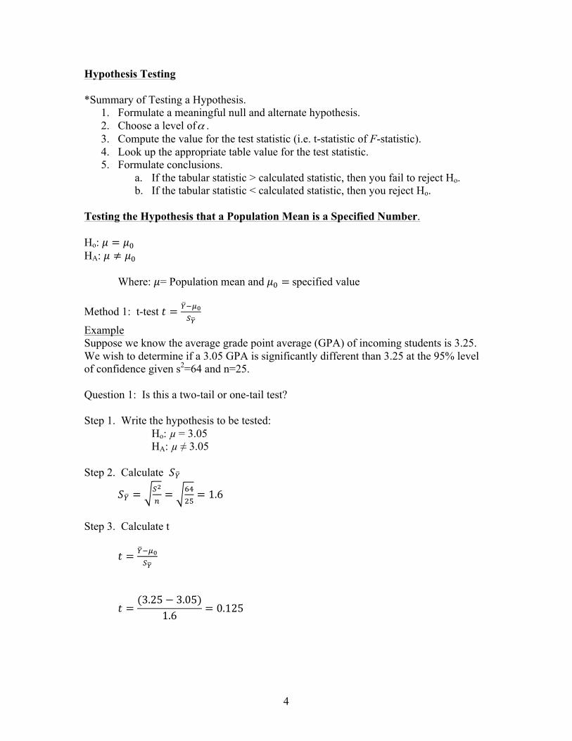
Hypothesis Testing *Summary of Testing a Hypothesis.

1. Formulate a meaningful null and alternate hypothesis. 2. Choose a level ofα . 3. Compute the value for the test statistic (i.e. t-statistic of F-statistic). 4. Look up the appropriate table value for the test statistic. 5. Formulate conclusions.

a. If the tabular statistic > calculated statistic, then you fail to reject Ho. b. If the tabular statistic < calculated statistic, then you reject Ho.

Testing the Hypothesis that a Population Mean is a Specified Number. Ho: 𝜇 = 𝜇! HA: 𝜇 ≠ 𝜇! Where: 𝜇= Population mean and 𝜇! =  specified value Method 1: t-test 𝑡 = !!!!

!!

Example Suppose we know the average grade point average (GPA) of incoming students is 3.25. We wish to determine if a 3.05 GPA is significantly different than 3.25 at the 95% level of confidence given s2=64 and n=25. Question 1: Is this a two-tail or one-tail test? Step 1. Write the hypothesis to be tested: Ho: µ = 3.05

HA: µ ≠ 3.05

Step 2. Calculate 𝑆!

𝑆! =!!

!= !"

!"= 1.6

Step 3. Calculate t 𝑡 = !!!!

!!

𝑡 =(3.25− 3.05)

1.6 = 0.125

5

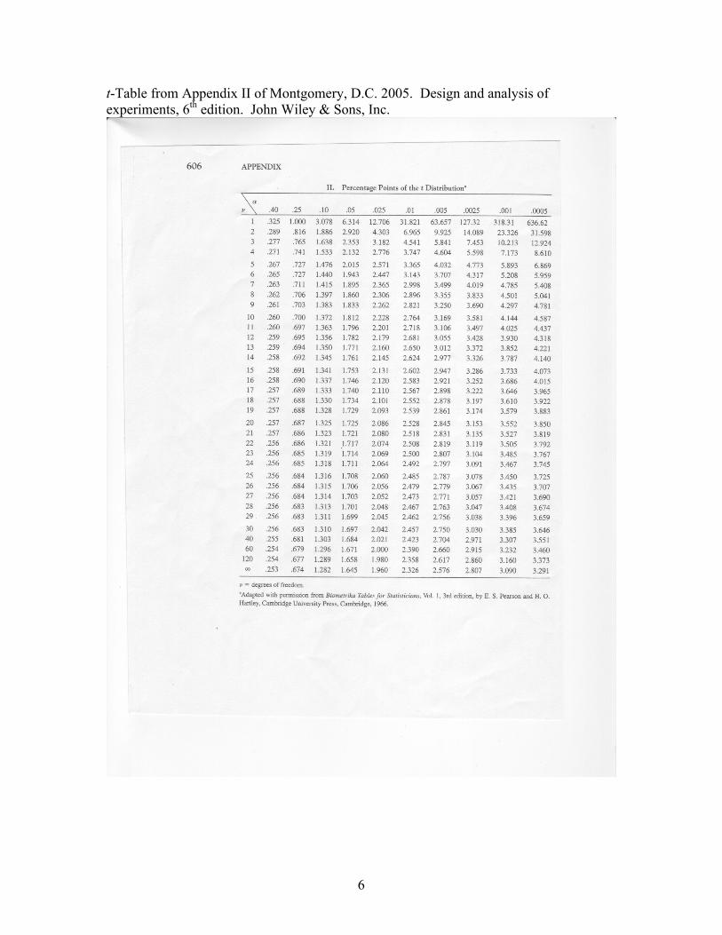
Step 4. Look up the Table t-value

§ Df = (n-1) = 25-1 = 24 § 2/α =0.05 (Note the two as the divisor of α is indicating that this is a two-tail

test. Thus, using the Appendix Table II of your text (Page 606), you need to use the column for α=0.025.

§ Table t-value=2.064.

Step 5. Make conclusions. -2.064 0.125 2.064 How would this problem have been different if this was a one-tail test? Step 1. Write the hypothesis to be tested: Ho: 05.3≤µ

HA: 05.3>µ

Step 2. Calculate Ys

6.125642

===nssY

Step 3. Calculate t 𝑡 = !!!!

!!

𝑡 =(3.25− 3.05)

1.6 = 0.125

Since t-calc (0.125) is < t-table (2.064) we fail to reject Ho: at the 95% level of confidence. Thus we can conclude that a GPA of 3.05 is not significantly different from 3.25 at the 95% level of confidence.

6

t-Table from Appendix II of Montgomery, D.C. 2005. Design and analysis of experiments, 6th edition. John Wiley & Sons, Inc.

7

Step 4. Look up the Table t-value

§ df = (n-1) = 25-1 = 24 § α =0.05 (Note there is no two as the divisor of α is indicating that this is a one-

tail test; thus, you should use the column in Appendix Table II for α=0.05.

§ Table t-value=1.711. Step 5. Make conclusions. 0.125 1.711 Confidence Intervals

§ An alternative method to test the hypothesis Ho: 0µµ = is to use a confidence interval (CI).

§ The hypotheses Ho: 0µµ = and HA: 0µµ ≠ can be rewritten as: Ho: 00 =−µµ and HA: 00 ≠−µµ .

§ Therefore, if the interval includes the value 0, we fail to reject the null hypothesis. § The formula for the CI to test Ho: 0µµ = is:

𝐶𝐼 = (𝜇 − 𝜇!)± 𝑡! !𝑆!

Example Using the numbers from the previous example:

302.320.0)6.1(064.2)05.325.3(

±=

±−=CI

Therefore: the lower limit l1 = -3.102 the upper limit l2 = 3.502 Since the interval includes the value 0, we fail to reject Ho: 00 =−µµ at the 95% level of confidence.

Since t-calc (0.125) is < t-table (1.711) we fail to reject Ho: at the 95% level of confidence. Thus we can conclude that a GPA of 3.05 is not less than 3.25 at the 95% level of confidence.

8

Comparison of Two Sample Means (t-test) Suppose we have two population means of 𝜇!  𝑎𝑛𝑑  𝜇! and we want to test the hypothesis: Ho: 21 µµ = HA: 21 µµ ≠

This can be done using a t-test where: 21

21

YYsYYt

−

−=

Where: 1Y = mean of treatment 1 2Y = mean of treatment 2

21 YYs −= standard deviation of the difference between two means.

§ Calculation of

21 YYs −depends on three things.

1. Do the populations have a common variance (i.e. 22

21 σσ = )?

2. Are the two samples of equal size (i.e. n1 = n2)? 3. Are the observations meaningfully paired?

*Comparisons of Two Sample Means (n1 = n2) and 2

221 σσ =

Given the following data:

iY∑ 2iY∑

Treatment 1 7 9 10 6 9 7 48 396 Treatment 2 2 5 3 1 5 2 18 68 Determine if the treatments means are significantly different at the 95% level of confidence. Step 1. Write the hypothesis to be tested: Ho: 21 µµ =

HA: 21 µµ ≠

9

Step 2. Calculate 22

21 & ss

s12 =396− 48

2

66−1

= 2.4

8.21661868

2

22 =

−

−=s

Step 2.1 Test to see if the two variances are homogeneous (i.e. Ho: 2

221 σσ = ).

• The method of calculating

21 YYs −will depend on whether you reject or fail to reject

Ho: 22

21 σσ = .

• If you fail to reject Ho: 22

21 σσ = , the formula for

21 YYs −is:

ns

s pYY

2221=−

where: 2

ps = the pooled variance and n = the number of observations in a treatment total.

• If you reject Ho: 22

21 σσ = , the formula for

21 YYs −is:

2

22

1

21

21 ns

nss YY +=−

where: 2

1s = variance of Treatment 1 2

2s = variance of Treatment 2 1n = number of observations for treatment 1 2n = number of observations for treatment 2

§ Test Ho: 2

221 σσ = using an F-test where:

2

2argσσ

SmallererLF =

10

§ If there are large differences between 2

221 & ss , F will become large and result in

the rejection of Ho: 22

21 σσ = .

§ We will be testing the hypothesis Ho: 2

221 σσ = at the 95% level of confidence.

§ This F-test is a two-tail test because we are not specifying which variance is

expected to be larger.

§ Thus, if you are testing 2/α = 0.05, then you need to use the F-table for α = 0.025 (Appendix Table IV, page 611).

§ This situation (i.e. testing Ho: 2

221 σσ = ) will be the only one used this semester in

which the F-test is a two-tail test.

§ When we use an F-test to test Ho: 21 µµ = , this will be a one-tail F-test because the numerator of the test, the variance based on means ( 22

Trσσ + ), is expected to

be larger than the denominator, the variance based on individual observations ( 2σ). This one-tail F-test requires use of Appendix Table IV on page 610.

• For this problem 167.14.28.2==F

Step 2.2 Look up table F-value in Appendix Table IV (pages 611).

§ F )1(),1(,2/ 21 −− nnα = F alpha value/2; numerator df, denominator df

§ The table in our text is set up for one-tail tests. Thus, to use the table for a two-

tail test and you want to test α at the 0.01 level, you need to look up the value of 0.005 in the table. The area under each of the two-tails is 0.005.

§ For this problem the table F for F0.05/2;5,5=7.15.

11

Part of F-Table from Appendix IV of Montgomery, D.C. 2005. Design and analysis of experiments, 6th edition. John Wiley & Sons

Step 2.3 Make conclusions: • Since the calculated value of F (1.167) is less than the Table-F value (7.15), we fail to

reject Ho: 22

21 σσ = at the 95% level of confidence.

• Therefore, we can calculate 21 YYs − using the formula:

ns

s pYY

2221=−

Step 3. Calculate 2

ps § The following formula will work in 21 nn = or 21 nn ≠

)1()1()1()1(

21

222

2112

−+−

−+−=

nnsnsnsp

where: 21s = variance of Treatment 1

22s = variance of Treatment 2

1n = number of observations for treatment 1 2n = number of observations for treatment 2

§ If 21 nn = , you can calculate 2ps using the formula

2

22

212 sssp+

=

§ For this problem 6.22

)8.24.2(2 =+

=ps

Step 4. Calculate 21 YYs −

§ The following formula will work in 21 nn = or 21 nn ≠

)11(21

221 nn

ss pYY +=−

§ If 21 nn = , you can calculate

21 YYs − using the formula:

ns

s pYY

2221=−

Where n = the number of observations in a treatment total.

§ For this problem 9309.06)6.2(2

21==−YYs

Step 5. Calculate t-statistic

21

21

YYsYYt

−

−=

371.5

9309.0/5

9309.0618

648

=

=

−=t

Step 6. Look up table t-value.

§ df= )1()1( 21 −+− nn =(6-1)+(6-1)=10

t.05/2;10df = 2.228 Step 6. Make conclusions. -2228 2.228 5.371

Since t-calc (5.371) is > t-table (2.228) we reject Ho: at the 95% level of confidence. Thus we can conclude that the mean of treatment 1 is significantly different than that of the mean of treatment 2at the 95% level of confidence.

Comparison of Two Sample Means (Confidence Interval)

§ The formula for a confidence interval to test the hypothesis: Ho: 21 µµ = is:

21221 )( YYstYY

−±− α

§ Using the data from the previous example:

21221 )( YYstYY

−±− α

07.793.207.25

)931.0(228.2)38(

2

1

=

=

±=

±−=

ll

Comparison of Two Sample Means (F-test)

§ In conducting tests of significance for: 21

21

::

µµ

µµ

≠

=

A

o

HH

we actually are conducting an F-

test of variances (i.e. the ratio of two variances.

F= estimate of σ2 based on means estimate of σ2 based on individuals

= 2

22

σσσ Tr+

§ When the null hypothesis is rejected, the numerator of the F-test becomes large as

compared to the denominator. This causes the calculated vale for F to become large. § So far in class we have seen two different ways to estimate 2σ :

1. nY /22 σσ =

§ We can estimate 2σ by n* 2Yσ (i.e. variance based on means).

2. We can estimate 2σ by calculating 2σ directly from individuals (variance based on

individuals).

Since the interval does not include the value 0, we must reject Ho:

at the 95% level of confidence.

§ The estimate of 2Yσ approaches 2σ only when you fail to reject Ho: because the treatment

effect 2Trσ in the expected mean square for the treatment source of variation ( 22

Trσσ + ) approaches zero.

§ When Ho: 21 µµ = is rejected and the treatment variances are homogenous (i.e. 22

21 σσ = ),

the estimate of 2σ based on means will over estimate 2σ . § This occurs because the estimate of 2σ based on means is affected by differences

between treatment means as well as differences due to random chance.

§ The estimate of 2σ based on individuals is not affected by differences between treatment means.

§ Note in the models below that the model for observations based on individuals does not

have a component for treatment.

§ This can be seen by looking at the linear models.

1. Linear model for observations based on individuals.

iiY εµ += Where: Yi = the ith observation of variable Y.

=µ population mean. iε = random error

2. Linear model for samples from two or more treatments.

ijiijY ετµ ++=

Where: Yij = the jth observation of the ith treatment. =µ population mean. iτ = the ith treatment

ijε = random error

§ We can estimate 2σ based on means by calculating a value called the Treatment Mean Square (TRT MS).

§ We can estimate 2σ based on individuals by calculating a value called the Error

Mean Square.

§ Given the linear model ijiijY ετµ ++= , we can rewrite the components as:

µ can be rewritten as ..Y

iτ can be rewritten as ... YY i −

ijε can be rewritten as .iij YY −

SOV Df SS MS F Among trt (Trt) t-1 2

... )( YYr i −∑ Trt SS/Trt df Trt MS/Error MS Within trt (Error) t(r-1) 2

. )( iij YY −∑ Error SS/Error df

Total tr-1 2.. )( YYij −∑

r = number of replicates t = number of treatments

Example § Using the data from the previous t-test and CI problem .iY 2

iY∑ Treatment 1 7 9 10 6 9 7 48 396 Treatment 2 2 5 3 1 5 2 18 68 Y..=66 Step 1. Calculate the Total SS

Total SS=( )rtY

YYY ijij ij

222

.. )(∑

−∑=−∑ Correction factor

Definition formula Working formula =(72 + 92 + 102 + . . . + 22) - 662/(6*2) = 464 – 363 = 101

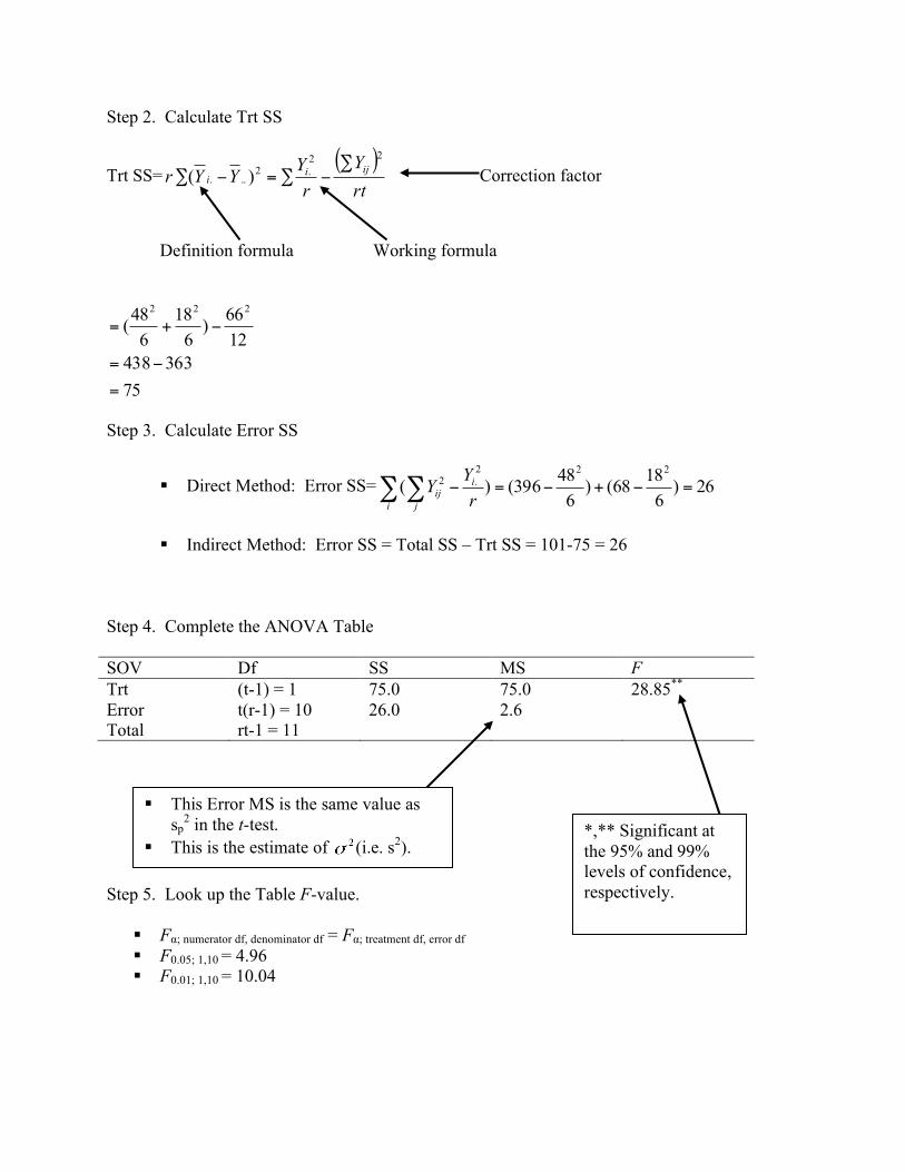
Step 2. Calculate Trt SS

Trt SS=( )rtY

rYYYr iji

i

22.2

... )(∑

−∑=−∑ Correction factor

Definition formula Working formula

75363438

1266)

618

648(

222

=

−=

−+=

Step 3. Calculate Error SS

§ Direct Method: Error SS= 26)61868()

648396()(

222.2 =−+−=−∑ ∑

i

i

jij rYY

§ Indirect Method: Error SS = Total SS – Trt SS = 101-75 = 26

Step 4. Complete the ANOVA Table SOV Df SS MS F Trt (t-1) = 1 75.0 75.0 28.85** Error t(r-1) = 10 26.0 2.6 Total rt-1 = 11 Step 5. Look up the Table F-value.

§ Fα; numerator df, denominator df = Fα; treatment df, error df § F0.05; 1,10 = 4.96 § F0.01; 1,10 = 10.04

§ This Error MS is the same value as sp

2 in the t-test. § This is the estimate of (i.e. s2).

*,** Significant at the 95% and 99% levels of confidence, respectively.

Step 6. Make conclusions. 0 4.96 10.04 28.85 Relationship Between the t-statistic and the F-statistic

§ When 22

21 σσ = , t2 = F.

Comparisons of Two Sample Means ( 21 nn ≠ ) and 2

221 σσ =

Given the following data:

iY∑ 2iY∑

Treatment 1 3 9 6 10 28 226 Treatment 2 11 15 9 12 12 13 72 884 Determine if the treatments means are significantly different at the 95% level of confidence. Step 1. Write the hypothesis to be tested: Ho: 21 µµ =

HA: 21 µµ ≠ Step 2. Calculate 2

221 & ss

1014428226

2

21 =

−

−=s

416672884

2

22 =

−

−=s

§ Since F-calc (28.85) > 4.96 we reject Ho: at the 95% level of confidence.

§ Since F-calc (28.85) > 10.04 we reject Ho: at the 99% level of confidence.

Step 2.1 Test to see if the two variances are homogeneous (i.e. Ho: 22

21 σσ = ).

2

2argσσ

SmallererLF =

• For this problem 5.2410

==F

Step 2.2 Look up table F-value in Appendix Table IV (page 611).

§ F )1(),1(,2/ 21 −− nnα = F alpha value/2; numerator df, denominator df

§ For this problem the table F for F0.05/2;3,5= 7.76.

Step 2.3 Make conclusions:

• Since the calculated value of F (2.5) is less than the Table-F value (7.76), we fail to reject Ho: 2

221 σσ = at the 95% level of confidence.

• Therefore, we can calculate 21 YYs − using the formula:

)11(21

221 nn

ss pYY +=−

Step 3. Calculate 2

ps

sp2 =(n1 −1)s1

2 + (n2 −1)s22

(n1 −1)+ (n2 −1)

where: 21s = variance of Treatment 1

22s = variance of Treatment 2

1n = number of observations for treatment 1 2n = number of observations for treatment 2

25.6)16()14(4)16(10)14(2 =

−+−−+−

=ps

Step 4. Calculate 21 YYs −

614.161

4125.6)11(

21

221

=⎟⎠

⎞⎜⎝

⎛ +=+=− nn

ss pYY

Step 5. Calculate t-statistic t = Y1 −Y2

sY1−Y2

098.3

614.1127

−=

−=t

§ Many people don’t line working with negative t-values. § If you are conducting a two-tail test, you can work with the absolute value of t since the

rejection regions are symmetrical about the axis of 0.

§ Therefore, 098.3098.3 =− Step 6. Look up table t-value.

§ Df= )1()1( 21 −+− nn =(4-1)+(6-1)=8

t.05/2;8df = 2.306 Step 6. Make conclusions. -2306 2.306 3.098

§ Since t-calc (3.098) is > t-table (2.306) we reject Ho: at the 95% level of confidence.

§ Thus we can conclude that the mean of treatment 1 is significantly different than that of the mean of treatment 2 at the 95% level of confidence.

Comparisons of Two Sample Means (n1 = n2 or 21 nn ≠ ) and 22

21 σσ ≠

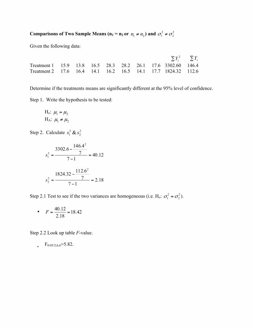
Given the following data: 2

iY∑ iY∑ Treatment 1 15.9 13.8 16.5 28.3 28.2 26.1 17.6 3302.60 146.4 Treatment 2 17.6 16.4 14.1 16.2 16.5 14.1 17.7 1824.32 112.6 Determine if the treatments means are significantly different at the 95% level of confidence. Step 1. Write the hypothesis to be tested: Ho: 21 µµ =

HA: 21 µµ ≠ Step 2. Calculate 2

221 & ss

12.401774.1466.33022

21 =

−

−=s

18.21776.11232.18242

22 =

−

−=s

Step 2.1 Test to see if the two variances are homogeneous (i.e. Ho: 2

221 σσ = ).

• 42.1818.212.40

==F

Step 2.2 Look up table F-value.

§ F0.05/2;6,6=5.82.

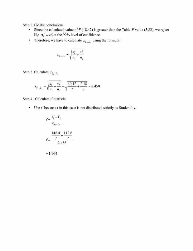
Step 2.3 Make conclusions: • Since the calculated value of F (18.42) is greater than the Table-F value (5.82), we reject

Ho: 22

21 σσ = at the 99% level of confidence.

• Therefore, we have to calculate 21 YYs − using the formula:

2

22

1

21

21 ns

nss YY +=

−

Step 3. Calculate

21 YYs −

458.2718.2

712.40

2

22

1

21

21=+=+=

− ns

nss YY

Step 4. Calculate t’-statistic

§ Use t’ because t in this case is not distributed strictly as Student’s t.

21

21'YYsYYt

−

−=

964.1

458.276.112

74.146

'

=

−=t

Step 5. Calculate effective degrees of freedom.

§ Calculation of the effective df allows us to use the t-table to look up values to test t’.

Effective df =

s12

n1+s22

n2

!

"#

$

%&

2

s12

n1

!

"#

$

%&

2

n1 −1( )

(

)

*****

+

,

-----

+

s22

n2

!

"#

$

%&

2

n2 −1( )

(

)

*****

+

,

-----

=

40.127

+2.187

!

"#

$

%&2

40.127

!

"#

$

%&2

7−1( )

(

)

****

+

,

----

+

2.187

!

"#

$

%&2

7−1( )

(

)

****

+

,

----

=36.516

(5.475+ 0.016)= 6.65

§ We can round the effective degrees of freedom of 6.65 to 7.0. § We then look up the t-value with 7 df.

§ t.05/2; 7df = 2.365

Step 6. Make conclusions. -2.365 1.964 2.365 Paired Comparisons • Earlier it was stated that calculation of

21 YYs − depends on three things:

4. Do the populations have a common variance (i.e. 22

21 σσ = )?

5. Are the two samples of equal size (i.e. n1 = n2)? 6. Are the observations meaningfully paired?

• We will now discuss the consequences of using paired comparisons. • Pairing of observations is done before the experiment is conducted.

§ Since t’-calc (1.964) is < t-table (2.365) we fail to reject Ho: at the 95% level of confidence.

§ Thus we can conclude that the mean of treatment 1 is not significantly different than that of the mean of treatment 2at the 95% level of confidence.

• Pairing is done to make the tests of significance more powerful. • If members of a pair tend to be large or small together, it may be possible to detect smaller

differences between treatments than would be possible without pairing. • The purpose of pairing is to eliminate an outside source of variation, that existing from pair

to pair. • Calculating the variance of differences rather than the variance of individuals controls the

variation. • Examples where pairing may be useful:

§ Drug or feed studies on the same animal. § Measurements done on the same individual at different times (before and after type

treatments).

• DD sD

sYYt =

−=

.2.1

• where nD

D ∑=

• ( )∑ ∑ −= jj YYD 21

• n = the number of pairs.

§ ns

nss DD

D ==2

• ( ) ( )[ ] ( )

11

22

2212

21

−

−=

−

−−−

=∑ ∑∑ ∑

nnD

D

nnYY

YYs

jjjj

D

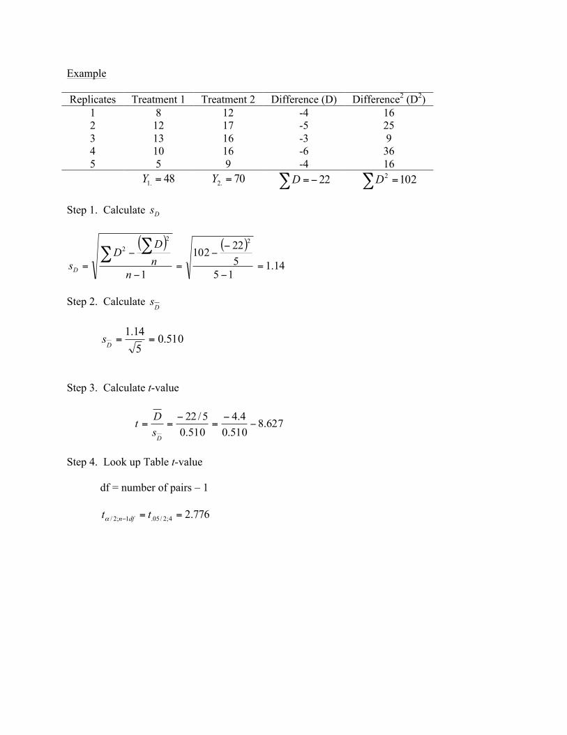
Example Replicates Treatment 1 Treatment 2 Difference (D) Difference2 (D2)

1 8 12 -4 16 2 12 17 -5 25 3 13 16 -3 9 4 10 16 -6 36 5 5 9 -4 16 48.1 =Y 70.2 =Y 22−=∑D ∑ =1022D

Step 1. Calculate Ds

( ) ( )14.1

15522102

1

222

=−

−−

=−

−=∑ ∑

nnD

DsD

Step 2. Calculate

Ds

510.0514.1

==Ds

Step 3. Calculate t-value

627.8510.04.4

510.05/22

−−

=−

==DsDt

Step 4. Look up Table t-value df = number of pairs – 1 776.24;2/05.1;2/ ==− tt dfnα

Step 5. Make conclusions -8.627 -2.776 2.776 REVIEW

• You might be thinking there are many formulas to remember; however, there are some simple ways to remember them.

• We have talked about four types of variances:

§ s2 = variance based on individuals § 2

Ys = variance based on means

§ 221 YYs − = variance of the difference between two means

§ 2Ds = variance of paired observations

• However, there is a relationship between all four variances that can help you in

remembering the formulas:

1/n s2 2

Ys

2 2/n 2 2Ds 2

21 YYs −

1/n

§ Since t-calc (-8.627) is < t-table (-2.776) we reject Ho: at the 95% level of confidence.

§ Thus we can conclude that the mean of treatment 1 is significantly different than that of the mean of treatment 2at the 95% level of confidence.

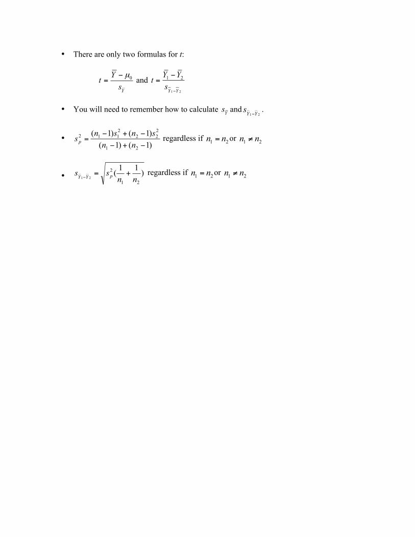
• There are only two formulas for t:

YsYt 0µ−= and

21

21

YYsYYt

−

−=

• You will need to remember how to calculate Ys and

21 YYs −.

• )1()1()1()1(

21

222

2112

−+−

−+−=

nnsnsnsp regardless if 21 nn = or 21 nn ≠

• )11(21

221 nn

ss pYY +=−

regardless if 21 nn = or 21 nn ≠

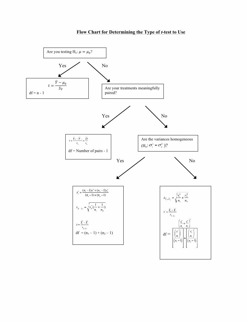
Flow Chart for Determining the Type of t-test to Use

Yes No

Yes No Yes No

df = Number of pairs - 1

Are the variances homogeneous (Ho: )?

df = (n1 – 1) + (n2 – 1)

𝑡 =𝑌! − 𝜇!𝑆!!

df = n - 1 Are your treatments meaningfully paired?

Are you testing Ho: 𝜇 = 𝜇!?

df =

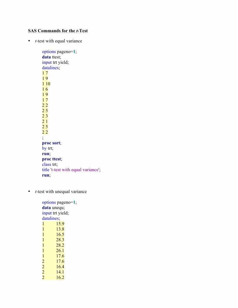
SAS Commands for the t-Test

• t-test with equal variance

options pageno=1; data ttest; input trt yield; datalines; 1 7 1 9 1 10 1 6 1 9 1 7 2 2 2 5 2 3 2 1 2 5 2 2 ; proc sort; by trt; run; proc ttest; class trt; title 't-test with equal variance'; run;

• t-test with unequal variance

options pageno=1; data unequ; input trt yield; datalines; 1 15.9 1 13.8 1 16.5 1 28.3 1 28.2 1 26.1 1 17.6 2 17.6 2 16.4 2 14.1 2 16.2

2 16.5 2 14.1 2 17.7 ;; proc sort; by trt; run; proc ttest; class trt; title 't-test with unequal variance'; run;

• Paired t-test

options pageno=1; data paired; input a b; datalines; 8 12 12 17 13 16 10 16 5 9 ;; proc ttest; paired a*b; title 'paired t-test'; run;

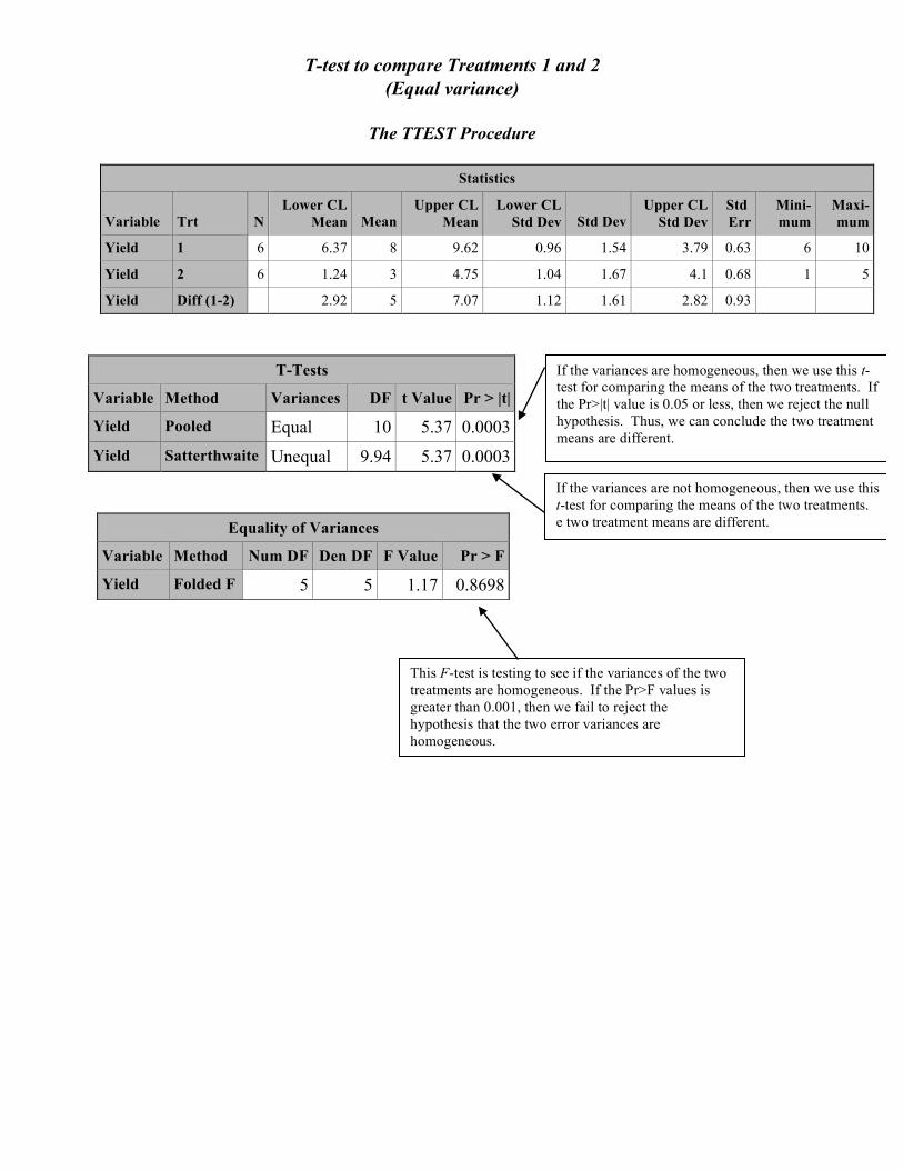
T-test to compare Treatments 1 and 2 (Equal variance)

The TTEST Procedure

Statistics

Variable Trt N Lower CL

Mean Mean Upper CL

Mean Lower CL

Std Dev Std Dev Upper CL

Std Dev Std Err

Mini-mum

Maxi-mum

Yield 1 6 6.37 8 9.62 0.96 1.54 3.79 0.63 6 10

Yield 2 6 1.24 3 4.75 1.04 1.67 4.1 0.68 1 5

Yield Diff (1-2) 2.92 5 7.07 1.12 1.61 2.82 0.93

T-Tests

Variable Method Variances DF t Value Pr > |t|

Yield Pooled Equal 10 5.37 0.0003 Yield Satterthwaite Unequal 9.94 5.37 0.0003

Equality of Variances

Variable Method Num DF Den DF F Value Pr > F

Yield Folded F 5 5 1.17 0.8698

If the variances are homogeneous, then we use this t-test for comparing the means of the two treatments. If the Pr>|t| value is 0.05 or less, then we reject the null hypothesis. Thus, we can conclude the two treatment means are different.

If the variances are not homogeneous, then we use this t-test for comparing the means of the two treatments. e two treatment means are different.

This F-test is testing to see if the variances of the two treatments are homogeneous. If the Pr>F values is greater than 0.001, then we fail to reject the hypothesis that the two error variances are homogeneous.

T-test to compare Treatments 1 and 2 (Unequal variance)

The TTEST Procedure

trt N Mean Std Dev Std Err Minimum Maximum

1 7 20.9143 6.3344 2.3942 13.8000 28.3000 2 7 16.0857 1.4758 0.5578 14.1000 17.7000 Diff (1-2) 4.8286 4.5991 2.4583

trt Method Mean 95% CL Mean Std Dev 95% CL Std Dev

1 20.9143 15.0559 26.7726 6.3344 4.0819 13.9488 2 16.0857 14.7208 17.4506 1.4758 0.9510 3.2499 Diff (1-2) Pooled 4.8286 -0.5276 10.1848 4.5991 3.2979 7.5918 Diff (1-2) Satterthwaite 4.8286 -1.0471 10.7042

Method Variances DF t Value Pr > |t|

Pooled Equal 12 1.96 0.0731 Satterthwaite Unequal 6.6495 1.96 0.0924

Equality of Variances

Method Num DF Den DF F Value Pr > F

Folded F 6 6 18.42 0.0025

T-test to compare Treatments 1 and 2 (Unequal variance)

The TTEST Procedure

N Mean Std Dev Std Err Minimum Maximum

5 -4.4000 1.1402 0.5099 -6.0000 -3.0000

Mean 95% CL Mean Std Dev 95% CL Std Dev

-4.4000 -5.8157 -2.9843 1.1402 0.6831 3.2764

DF t Value Pr > |t|

4 -8.63 0.0010

11

Part of F-Table from Appendix IV of Montgomery, D.C. 2005. Design and analysis of experiments, 6th edition. John Wiley & Sons