1

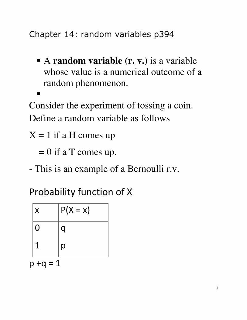
Chapter 14: random variables p394

� A random variable (r. v.) is a variable

whose value is a numerical outcome of a

random phenomenon.

� Consider the experiment of tossing a coin.

Define a random variable as follows

X = 1 if a H comes up

= 0 if a T comes up.

- This is an example of a Bernoulli r.v.

Probability function of X

x P(X = x)

0

1

q

p

p +q = 1

2

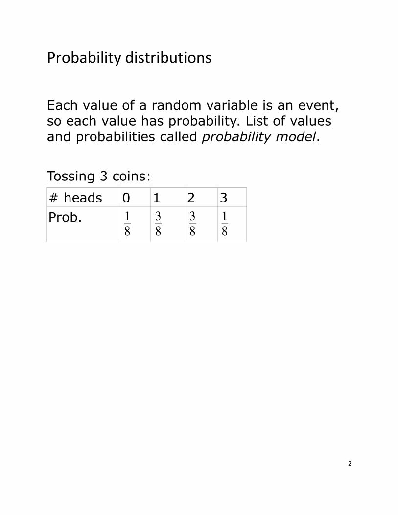
Probability distributions

Each value of a random variable is an event,

so each value has probability. List of values and probabilities called probability model.

Tossing 3 coins:

# heads 0 1 2 3

Prob. 1

8 3

8 3

8 1

8

3

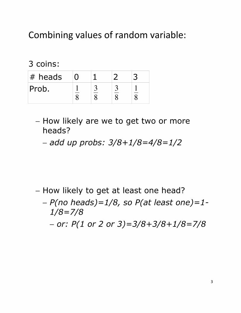
Combining values of random variable:

3 coins:

# heads 0 1 2 3

Prob. 1

8 3

8 3

8 1

8

− How likely are we to get two or more

heads?

− add up probs: 3/8+1/8=4/8=1/2

− How likely to get at least one head?

− P(no heads)=1/8, so P(at least one)=1-1/8=7/8

− or: P(1 or 2 or 3)=3/8+3/8+1/8=7/8

4

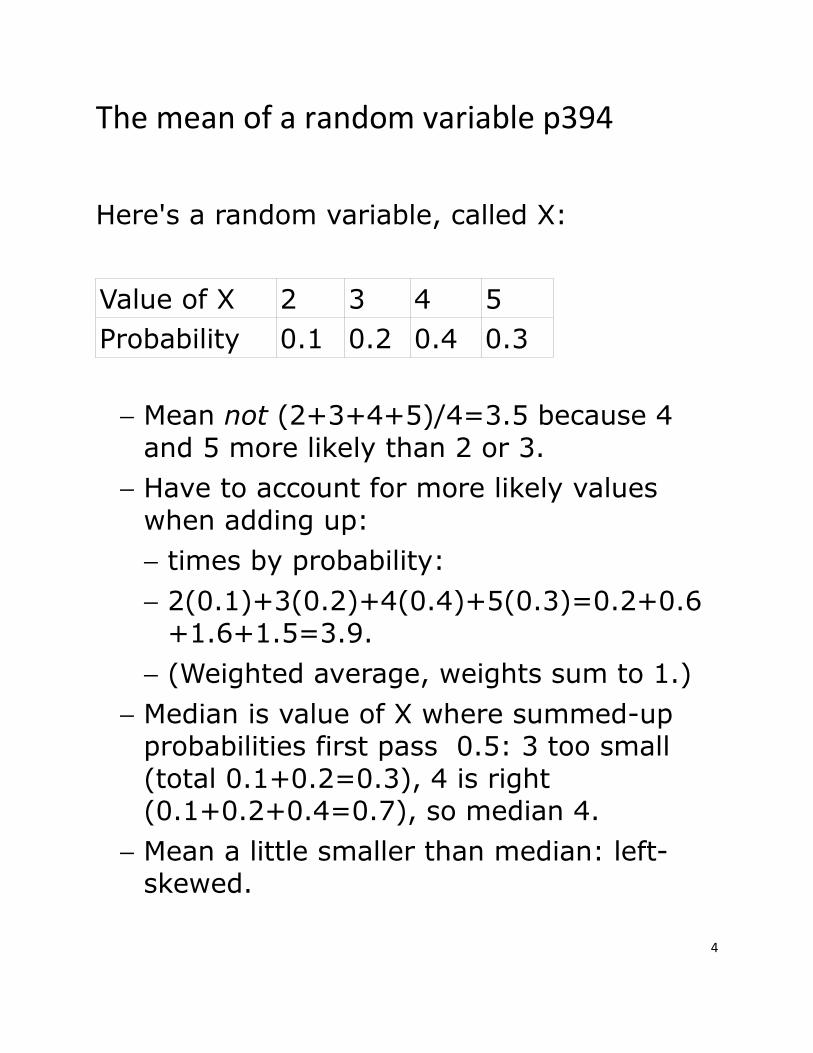
The mean of a random variable p394

Here's a random variable, called X:

Value of X 2 3 4 5

Probability 0.1 0.2 0.4 0.3

− Mean not (2+3+4+5)/4=3.5 because 4

and 5 more likely than 2 or 3.

− Have to account for more likely values

when adding up:

− times by probability:

− 2(0.1)+3(0.2)+4(0.4)+5(0.3)=0.2+0.6+1.6+1.5=3.9.

− (Weighted average, weights sum to 1.)

− Median is value of X where summed-up probabilities first pass 0.5: 3 too small

(total 0.1+0.2=0.3), 4 is right (0.1+0.2+0.4=0.7), so median 4.

− Mean a little smaller than median: left-skewed.

5

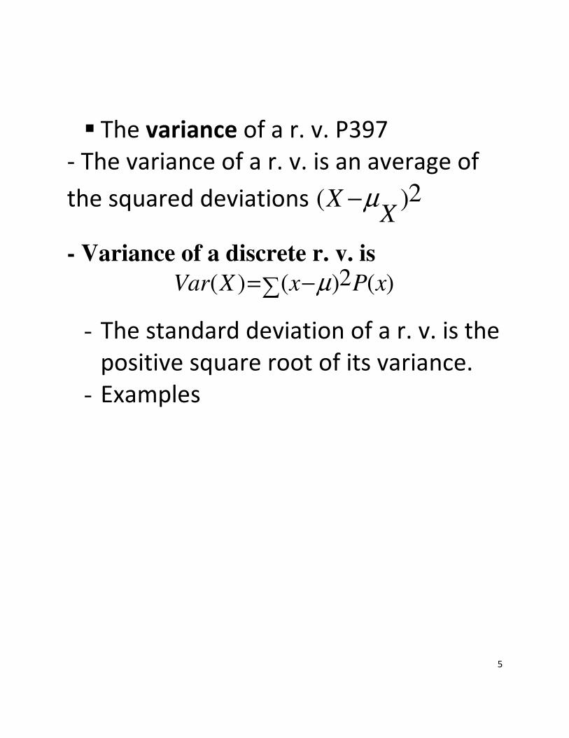
� The variance of a r. v. P397

- The variance of a r. v. is an average of

the squared deviations 2( )XX

µ−

- Variance of a discrete r. v. is 2( ) ( ) ( )Var X x P xµ= −∑

- The standard deviation of a r. v. is the

positive square root of its variance.

- Examples

6

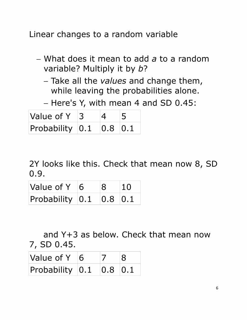
Linear changes to a random variable

− What does it mean to add a to a random

variable? Multiply it by b?

− Take all the values and change them,

while leaving the probabilities alone.

− Here's Y, with mean 4 and SD 0.45:

Value of Y 3 4 5

Probability 0.1 0.8 0.1

2Y looks like this. Check that mean now 8, SD

0.9.

Value of Y 6 8 10

Probability 0.1 0.8 0.1

and Y+3 as below. Check that mean now

7, SD 0.45.

Value of Y 6 7 8

Probability 0.1 0.8 0.1

7

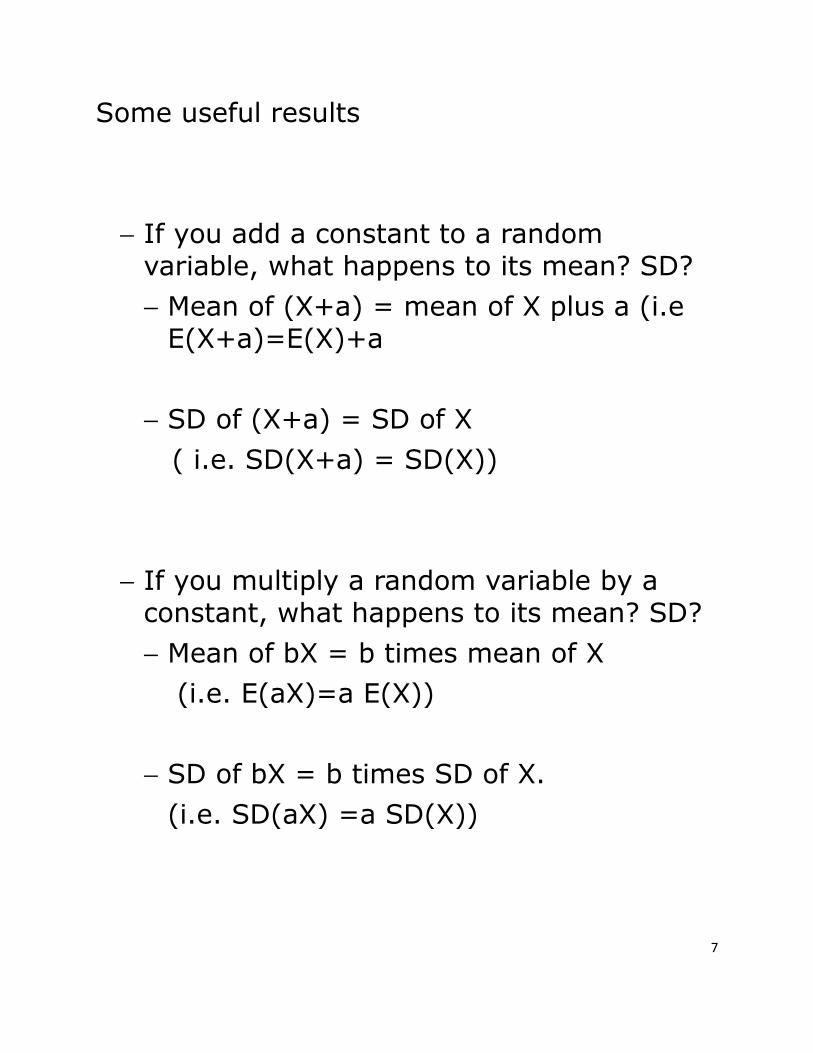
Some useful results

− If you add a constant to a random variable, what happens to its mean? SD?

− Mean of (X+a) = mean of X plus a (i.e E(X+a)=E(X)+a

− SD of (X+a) = SD of X

( i.e. SD(X+a) = SD(X))

− If you multiply a random variable by a constant, what happens to its mean? SD?

− Mean of bX = b times mean of X

(i.e. E(aX)=a E(X))

− SD of bX = b times SD of X.

(i.e. SD(aX) =a SD(X))

8

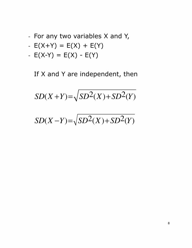
- For any two variables X and Y,

- E(X+Y) = E(X) + E(Y)

- E(X-Y) = E(X) - E(Y)

If X and Y are independent, then

2 2( ) ( ) ( )SD X Y SD X SD Y+ = +

2 2( ) ( ) ( )SD X Y SD X SD Y− = +

9

Continuous random variables

− So far: our random variables discrete: set

of possible values, like 1,2,3,... ,

probability for each.

− Recall normal distribution: any decimal

value possible, can't talk about probability of any one value, just eg. “less than 10”,

“between 10 and 15”, “greater than 15”.

− Normal random variable example of

continuous.

− Finding mean and SD of continuous

random variable involves calculus :-(

− but if we are given mean/SD, work as above.

10

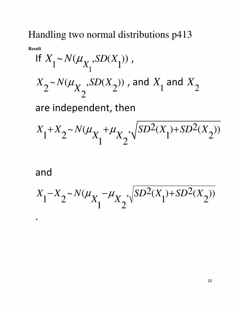
Handling two normal distributions p413

Result

If 1

1( )

1~ ( , )

XSD XX N µ ,

~ ( , ( ))2 2

2

X N SD XX

µ , and 1

X and 2

X

are independent, then

2 2~ ( , ( ) ( ))1 2 1 2

1 2

X X N SD X SD XX X

µ µ+ + +

and

2 2~ ( , ( ) ( ))1 2 1 2

1 2

X X N SD X SD XX X

µ µ− − +

.

11

Example

The weight of the empty box has a

normal distribution with mean 1kg and

std. dev. 100g. The weight of its

contents has a normal distribution with

mean 12kg and std. dev. 1.34 kg,

independently of the box.

Find the probability that the total

weight of the box and its contents will

exceed 15kg.

12

Ex. Two friends T and H run a race. H is

a faster runner and the time he takes

to complete is normally distributed

with mean 3 minutes with a std. dev.

30 sec. T’s time to complete the race is

normally distributed with mean 5

minutes and std. dev. 1 minute.

Find the probability that T will win the

race.

Ans.

P(T<H)= P(T-H<0)=P(Z<(0-(5-3))/sqrt(1.25))=P(Z<-1.79)= 0.0367

13

How do you find SD of sum and difference if

random variables are not independent?

− In this course, you don't.

− See p. 404 of text for gory details.

14

Probability Models p 405

The Binomial Model

Example:

A biased coin (P(H) = p = 0.6) ) is tossed 5

times. Let X be the number of H’s. Fine

P(X = 2).

This X is a binomial r. v.

15

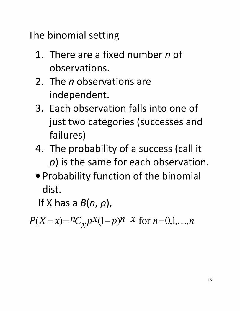
The binomial setting

1. There are a fixed number n of

observations.

2. The n observations are

independent.

3. Each observation falls into one of

just two categories (successes and

failures)

4. The probability of a success (call it

p) is the same for each observation.

• Probability function of the binomial

dist.

If X has a B(n, p),

( ) (1 ) for 0,1, ,n x n xP X x C p p n nx−= = − = …

16

Binomial table

The link to Statistical Tables on course

website includes table of binomial distribution probabilities. In here, find chance of exactly k

successes in n trials with success prob p.

Ex.

The probability that a certain machine will

produce a defective item is 1/5. If a random

sample of 6 items is taken from the output of this machine, what is the probability that

there will be 5 or more defectives in the sample?

17

Ex There are 20 multiple-choice questions

on an exam, each having responses a, b, c,

d and e. Each question is worth 5 points.

And only one response per question is

correct. Suppose that a student guesses

the answer to question and her guesses

from question to question are

independent. It the student needs at least

40 points to pass the test. What is the

probability that the student will pass the

test?

Ans. X~B(20, 0.2). P(X>=8) = 0.0322, adding the entries 8 through 20 in the appropriate of the binomial table

What is the expected (mean) score for this student. (later)

Ans. 20 x 0.2 = 4 and expected score =5 x 4= 20

18

Suppose n=8 and p=0.7. What is the

probability of

− exactly 7 successes?

− 7 or more successes?

Idea: count failures instead of successes.

P(success)=0.7 means P(failure)=1-0.7=0.3

7 successes = 8-7=1 failure.

so look up n=8, p=0.3, k=1 prob=0.1977

which is answer we want.

7 or successes = 7, 8 successes

P(failure)=1-0.7=0.3

7, 8 successes = 1, 0 failures

prob we want is 0.1977+0.0576=0.2553.

19

• Mean and Variance of a binomial r. v. p

If X has a Bin(n, p)

mean np= and (1 )SD np p= −

Example

20

0 1 2 3 4 5

0.0

50

.10

0.1

50

.20

0.2

50

.30

Binomial Distribution: Binomial trials=5, Probability of success=0.5

Number of Successes

Pro

ba

bility M

ass

21

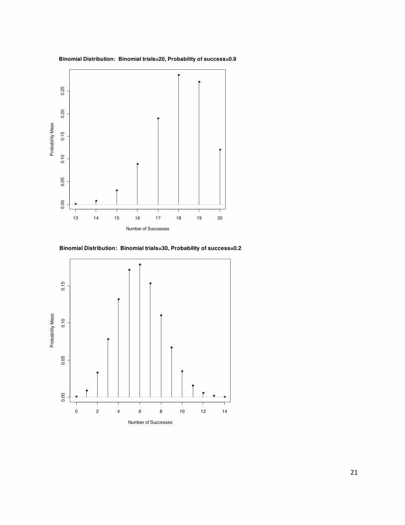
13 14 15 16 17 18 19 20

0.0

00

.05

0.1

00

.15

0.2

00.2

5Binomial Distribution: Binomial trials=20, Probability of success=0.9

Number of Successes

Pro

bab

ility M

ass

0 2 4 6 8 10 12 14

0.0

00

.05

0.1

00

.15

Binomial Distribution: Binomial trials=30, Probability of success=0.2

Number of Successes

Pro

bab

ility M

ass

22

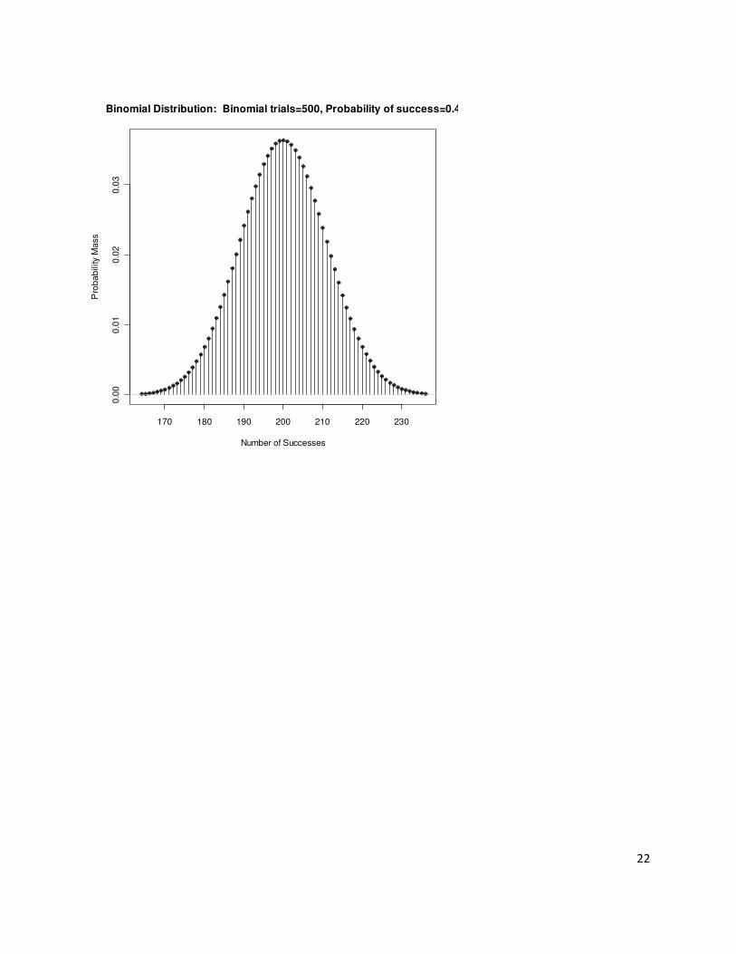
170 180 190 200 210 220 230

0.0

00.0

10

.02

0.0

3Binomial Distribution: Binomial trials=500, Probability of success=0.4

Number of Successes

Pro

bab

ility M

ass

23

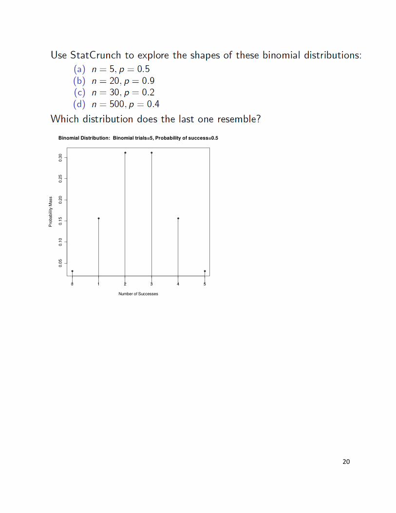
How does the shape depend on p?

p<0.5, skewed right;

p>0.5, skewed left;

p=0.5, symmetric

What happens to the shape as n increases?

− shape becomes normal

What does this suggest to do if n is too large

for the tables?

If n too large for tables, try normal approximation to binomial.

Compute mean and SD of binomial, then

pretend binomial actually normal:

24

• Normal approximation for counts and

proportions p415

Draw a SRS of size n from a large population

having population p of success. Let X be the

count of success in the sample and ˆ /p X n=

the sample proportion of successes. When

n is large, the sampling distributions of

these statistics are approximately normal:

X is approx. ( , (1 ))N np np p−

Works if n large and p not too far from 0.5

As a rule of thumb, we will use this

approximation for values of n and p

that satisfy 10np≥ and (1 ) 10n p− ≥ .

can relax this a bit if p close to 0.5.

25

According to government data, 21% of

American children under the age of six live

in households with incomes less than the

official poverty level. A study of learning in

early childhood chooses an SRS of 300

children.

(a) What is the mean number of children in

the sample who come from poverty-level

households?

What is the standard deviation of this

number?

(b) Use the normal approximation to

calculate the probability that at least 80 of

the children in the sample live in poverty.

Be sure to check that you can safely use the

approximation.

(a) µ = (300)(0.21) = 63, σ = )79.0)(21.0)(300( = 7.0548. (b) np = 63 and n(1–p) = 237 are both more

than 10, so we may approximate using the normal distribution: P(X ≥ 80) = P(Z ≥ 2.41) = 0.0080, or with

the continuity correction: P(X ≥ 79.5) = P(Z ≥ 2.34) = 0.0096.