Manual ver. 4.2.1, 27 February 2016

HITRAN Application Programming Interface

(HAPI)

User Guide

Roman V. Kochanov

rkochanov@cfa.harvard.edu

Harvard-Smithsonian Center for Astrophysics

Atomic and Molecular Physics Division

60 Garden St, Cambridge MA 02138, USA

2

Table of Contents

I. INTRODUCTION ....................................................................................................................... 3

1.1. PREFACE ............................................................................................................................ 3

1.2. FEATURES SUMMARY ...................................................................................................... 3

II. PREREQUISITES ...................................................................................................................... 4

III. WORKING WITH DATA ......................................................................................................... 5

3.1. LOCAL DATABASE STRUCTURE ...................................................................................... 5

3.2. DOWNLOADING AND DESCRIBING DATA .................................................................... 5

3.3. FILTERING AND OUTPUTTING DATA .......................................................................... 11

3.4. FILTERING CONDITIONS ............................................................................................... 12

3.5. ACCESSING COLUMNS IN A TABLE .............................................................................. 14

3.6. SPECIFYING A LIST OF PARAMETERS ......................................................................... 15

3.7. SAVING QUERY TO DISK ................................................................................................ 15

3.8. GETTING INFORMATION ON ISOTOPOLOGUES ....................................................... 16

IV. CALCULATING SPECTRA ................................................................................................... 17

4.1. USING LINE PROFILES................................................................................................... 17

4.2. USING PARTITION SUMS ................................................................................................ 19

4.3. CALCULATING ABSORPTION COEFFICIENTS ........................................................... 20

4.4. CALCULATING ABSORPTION, TRANSMITTANCE, AND RADIANCE SPECTRA ....... 25

4.5. APPLYING INSTRUMENTAL FUNCTIONS .................................................................... 26

4.6. ALIASES ............................................................................................................................ 29

V. PLOTTING WITH MATPLOTLIB .......................................................................................... 31

VI. KEY FUNCTIONS: EXAMPLES .......................................................................................... 37

6.1. Help system ........................................................................................................................ 38

6.2. Fetching data ..................................................................................................................... 38

6.3. Working with data .............................................................................................................. 39

6.4. Calculating spectra............................................................................................................ 43

6.5. Convolving spectra ............................................................................................................ 49

6.6. Information on isotopologues ............................................................................................ 51

6.7. Miscellaneous .................................................................................................................... 54

REFERENCES: ............................................................................................................................. 55

3

I. INTRODUCTION

1.1. PREFACE

HITRAN Application Programming Interface (HAPI) is a set of routines in Python which is aimed to

provide a remote access to functionality and data given by the new project HITRANonline

(http://hitran.org)1.

At the present time, the API can download, filter and process data on molecular and atomic line-by-line

spectra which is provided by the HITRANonline portal.

One of the major purposes of introducing this API is to extend the functionality of the main site,

particularly providing a possibility to calculate several types of spectral functions based on the flexible

HT (Hartmann-Tran) profile [1] and optionally accounting for instrumental functions.

Each feature of the API is represented by a Python function with a set of parameters providing a

flexible approach to the task.

The current version is at the beta stage. All comments and suggestions are welcome!

The HAPI library doesn't require installation by itself. The user just needs to install prerequisites (see

Section II).

HAPI is a free product and uses only open-source libraries. It goes under Academic Free License. More

information about HAPI versions and licensing can be found at Zenodo community:

https://zenodo.org/collection/user-hapi

1.2. FEATURES SUMMARY

Some of the prominent current features of HAPI are:

1) Downloading line-by-line data from the HITRANonline site to a local machine.

2) Filtering and processing the data in SQL-like fashion.

3) Conventional Python structures (lists, tuples, and dictionaries) for representing spectroscopic data.

4) Possibility to use a large set of third-party Python libraries to work with the data.

5) Python implementation of the HT profile [1-3] which can be used in spectra simulations. This line

shape can also be reduced to a number of conventional line profiles such as Gaussian (Doppler),

Lorentzian, Voigt, Rautian, Speed-dependent Voigt and speed-dependent Rautian.

6) Python implementation of total internal partition sums (TIPS-2011 [4]) which is used in spectra

simulations as well as scaling some HITRAN [5] parameters.

7) High-resolution spectra simulation accounting for pressure, temperature and optical path length.

The following spectral functions can be calculated:

a) absorption coefficient b) absorption spectrum

c) transmittance spectrum d) radiance spectrum

8) Spectral calculation using a number of instrumental functions to simulate experimental spectra.

9) Possibility to extend the user's functionality by adding custom line shapes, partition sums and

apparatus functions.

1 Currently redirects to http://hitranazure.cloudapp.net.

4

II. PREREQUISITES

HITRAN API has the following two prerequisites:

1) Python 2.6+:

https://www.python.org/

2) Numpy:

http://www.numpy.org/

These two entities can be installed either separately (see the links given) or in one shot using a

scientific Python distribution:

http://continuum.io/downloads (“Anaconda”)

https://www.enthought.com/products/canopy (“Canopy”)

http://www.sagemath.org (“Sage”)

… or any other similar package.

To be able to go through tutorials the user would need to have the Matplotlib installed:

http://matplotlib.org/

To have a nice Mathematica-style interface for Python the user can install IPython notebook:

http://ipython.org/

Note that all listed prerequisites are open source and free to use.

5

III. WORKING WITH DATA

Welcome to the manual on retrieving and processing the data from HITRANonline.

This manual will give you an insight of how to use HAPI's capabilities for working with data.

3.1. LOCAL DATABASE STRUCTURE

The local data is downloaded from the HITRANonline portal (http://hitran.org) using API functions

(fetch and fetch_by_ids). Downloaded data is stored in the folder which was specified in a call to

db_begin().

The structure of a local data folder is as follows (assuming that you have already downloaded several

tables from HITRANonline):

Folder name

|

|----- table1.data

| table1.header

|

|----- table2.data

| table2.header

…

|----- tableN.data

tableN.header

The typical format is as follows: <table_name>.data for line-by-line data, and <table_name>.header

for table description (field names and positions, format, number of lines etc...). The default file format

is 160-character HITRAN format (see Ref [5] and links within).

Besides working with downloaded HITRANonline data, HAPI can also deal with custom data files. It

is sufficient to copy HITRAN-formatted files with an extension “.par” into the database directory, and

HAPI will detect them automatically after the db_begin() call.

3.2. DOWNLOADING AND DESCRIBING DATA

To start working with HAPI, the user should import all functions from the module “hapi.py”:

from hapi import *

First, let's choose a folder for our local database. Every time you start your Python project, you have to

specify explicitly the name of the database folder.

6

db_begin('data')

N.B. It's important to note that commands in Python are case sensitive!

So, let's download some data from the server and do some processing on it. Suppose that we want to

get line-by-line data on the main isotopologue of H2O.

For retrieving the data to the local database, the user has to specify the following parameters:

1) Name of the local table which will store the downloaded data.

2) Either a pair of molecule and isotopologue HITRAN numbers (M and I), or a "global" isotopologue

ID (iso_id).

3) Wavenumber range (nu_min and nu_max)

N.B. If you specify a name which already exists in your local folder, the existing table with that name

will be overwritten.

To get additional information on function fetch, call getHelp:

getHelp(fetch)

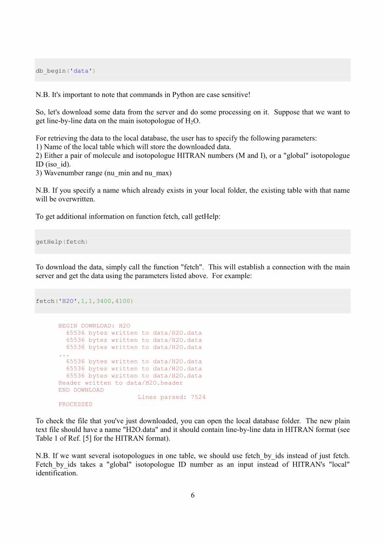
To download the data, simply call the function "fetch". This will establish a connection with the main

server and get the data using the parameters listed above. For example:

fetch('H2O',1,1,3400,4100)

BEGIN DOWNLOAD: H2O 65536 bytes written to data/H2O.data 65536 bytes written to data/H2O.data 65536 bytes written to data/H2O.data ... 65536 bytes written to data/H2O.data 65536 bytes written to data/H2O.data 65536 bytes written to data/H2O.data Header written to data/H2O.header END DOWNLOAD Lines parsed: 7524 PROCESSED

To check the file that you've just downloaded, you can open the local database folder. The new plain

text file should have a name "H2O.data" and it should contain line-by-line data in HITRAN format (see

Table 1 of Ref. [5] for the HITRAN format).

N.B. If we want several isotopologues in one table, we should use fetch_by_ids instead of just fetch.

Fetch_by_ids takes a "global" isotopologue ID number as an input instead of HITRAN's "local"

identification.

7

See getHelp(fetch_by_ids) to get more information on this.

To get a list of tables which are already in the database, use the tableList() function (it takes no

arguments):

tableList()

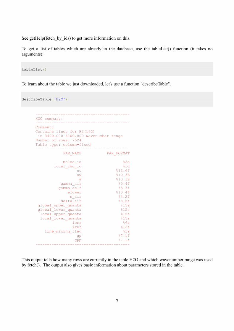
To learn about the table we just downloaded, let's use a function "describeTable".

describeTable('H2O')

----------------------------------------- H2O summary: ----------------------------------------- Comment: Contains lines for H2(16O) in 3400.000-4100.000 wavenumber range Number of rows: 7524 Table type: column-fixed ----------------------------------------- PAR_NAME PAR_FORMAT molec_id %2d local_iso_id %1d nu %12.6f sw %10.3E a %10.3E gamma_air %5.4f gamma_self %5.3f elower %10.4f n_air %4.2f delta_air %8.6f global_upper_quanta %15s global_lower_quanta %15s local_upper_quanta %15s local_lower_quanta %15s ierr %6s iref %12s line_mixing_flag %1s gp %7.1f gpp %7.1f -----------------------------------------

This output tells how many rows are currently in the table H2O and which wavenumber range was used

by fetch(). The output also gives basic information about parameters stored in the table.

8

PARAMETERS AND PARAMETER GROUPS

Since the ver. 1.1 HAPI provides a feature of querying “non-standard” parameters, i.e. those not being

a part of 160-character HITRAN format. To query a specific parameter one still needs to use either

fetch() of fetch_by_ids(). For this purpose two additional arguments are introduced: Parameters and

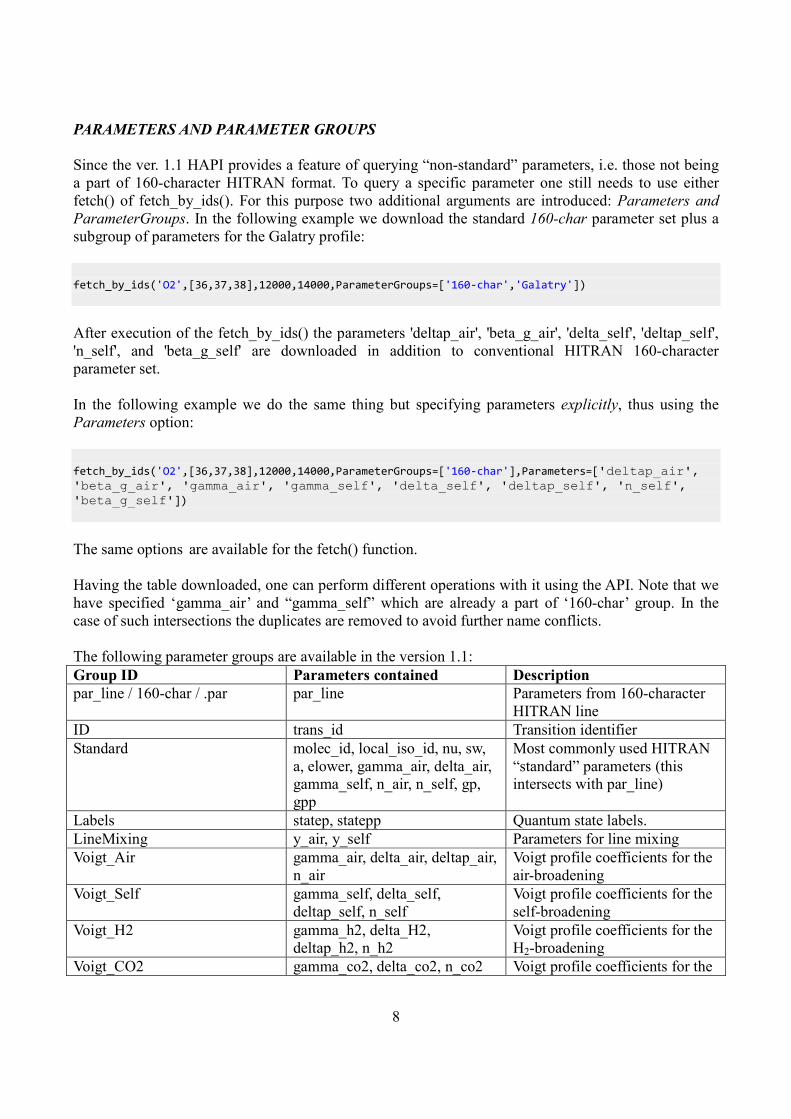
ParameterGroups. In the following example we download the standard 160-char parameter set plus a

subgroup of parameters for the Galatry profile:

fetch_by_ids('O2',[36,37,38],12000,14000,ParameterGroups=['160-char','Galatry'])

After execution of the fetch_by_ids() the parameters 'deltap_air', 'beta_g_air', 'delta_self', 'deltap_self',

'n_self', and 'beta_g_self' are downloaded in addition to conventional HITRAN 160-character

parameter set.

In the following example we do the same thing but specifying parameters explicitly, thus using the

Parameters option:

fetch_by_ids('O2',[36,37,38],12000,14000,ParameterGroups=['160-char'],Parameters=['deltap_air', 'beta_g_air', 'gamma_air', 'gamma_self', 'delta_self', 'deltap_self', 'n_self', 'beta_g_self'])

The same options are available for the fetch() function.

Having the table downloaded, one can perform different operations with it using the API. Note that we

have specified ‘gamma_air’ and “gamma_self” which are already a part of ‘160-char’ group. In the

case of such intersections the duplicates are removed to avoid further name conflicts.

The following parameter groups are available in the version 1.1:

Group ID Parameters contained Description

par_line / 160-char / .par par_line Parameters from 160-character

HITRAN line

ID trans_id Transition identifier

Standard molec_id, local_iso_id, nu, sw,

a, elower, gamma_air, delta_air,

gamma_self, n_air, n_self, gp,

gpp

Most commonly used HITRAN

“standard” parameters (this

intersects with par_line)

Labels statep, statepp Quantum state labels.

LineMixing y_air, y_self Parameters for line mixing

Voigt_Air gamma_air, delta_air, deltap_air,

n_air

Voigt profile coefficients for the

air-broadening

Voigt_Self gamma_self, delta_self,

deltap_self, n_self

Voigt profile coefficients for the

self-broadening

Voigt_H2 gamma_h2, delta_H2,

deltap_h2, n_h2

Voigt profile coefficients for the

H2-broadening

Voigt_CO2 gamma_co2, delta_co2, n_co2 Voigt profile coefficients for the

9

CO2- broadening

Voigt_He gamma_he, delta_he, n_he Voigt profile coefficients for the

He-broadening

Voigt All Voigt parameters This group contains all Voigt-

related parameters

SDVoigt_Air gamma_air, delta_air, deltap_air,

n_air, sd_air

Speed-dependent Voigt profile

coefficients for the air-

broadening

SDVoigt_Self gamma_self, delta_self,

deltap_self, n_self, sd_self

Speed-dependent Voigt profile

coefficients for the self-

broadening

SDVoigt All SDVoigt parameters This group contains all Speed-

dependent Voigt-related

parameters

Galatry_Air gamma_air, delta_air, deltap_air,

n_air, beta_g_air

Galatry profile coefficients for

the air-broadening

Galatry_Self gamma_self, delta_self,

deltap_self, n_self, beta_g_self

Galatry profile coefficients for

the self-broadening

Galatry All Galatry parameters This group contains all Galatry-

related parameters

All All parameters at once

All accessible parameters are given in the table below. Note that since parameters are gradually being

added to the HITRAN database, this list can be incomplete. For a full parameter list one can refer to the

http://www.hitran.org site of to the latest HAPI user guide.

Parameter identifiers used in HAPI

Parameter Units Identifier Description

Parameters from the HITRAN2004 format in HITRANonline

Molecule ID – molec_id HITRAN integer identifying the

molecule

Isotopologue

ID

– local_iso_id HITRAN integer identifying the

isotopologue of a particular molecule

ɶυ cm-1

nu Transition wavenumber

S cm-1

/

(molec cm-2

)

sw Transition intensity, weighted by

isotopologue abundance

A s-1

a Einstein A-coefficient

airγ cm-1 atm-1 gamma_air Air-broadened Lorentzian HWHM

coefficient (for Voigt lineshape)

selfγ cm-1

atm-1

gamma_self Self-broadened Lorentzian HWHM

coefficient (for Voigt lineshape)

''E cm-1

elower Lower state energy

airn – n_air Temperature-dependence exponent for

airγ

10

airδ cm-1

atm-1

delta_air Air pressure-induced line shift

V ′ – global_upper_quanta Upper-state “global” quanta in

HITRAN 160-character format

V ′′ – global_lower_quanta Lower-state “global” quanta in

HITRAN 160-character format

Q′ – local_upper_quanta Upper-state “local” quanta in

HITRAN 160-character format

Q′′ – local_lower_quanta Lower-state “local” quanta in

HITRAN 160-character format

'g – gp Lower state statistical weight

''g – gpp Upper state statistical weight

Metadata and other special parameters

Transition ID – trans_id Unique integer identifying the

transition

Global

Isotopologue

ID

– global_iso_id Global integer ID identifying

the isotopologue (unique across the

whole database)

qns’ – statep Upper state quantum numbers in

HITRANonline format

qns’’ – statepp Lower state quantum numbers in

HITRANonline format

.par line – par_line Complete representation of the

line in the HITRAN2004 160-

character, .par format

Parameters for broadening by new perturbing species, X, and non-Voigt parameters

selfn – n_self Temperature-dependence exponent for

selfγ

selfδ cm-1

atm-1

delta_self Self-induced pressure line shift

airδ ′ cm-1 atm-1 K-1 deltap_air Linear temperature dependence

coefficient for airδ

selfδ ′ cm-1

atm-1

K-1

deltap_self Linear temperature dependence

coefficient for selfδ

Xγ cm-1

atm-1

gamma_X Lorentzian HWHM coefficient

(for Voigt lineshape) for broadening

by perturber X ♦

Xn – n_X Temperature-dependence exponent

for Xγ

Xδ cm-1 atm-1 delta_X Pressure-induced line shift due

to perturber X

0 ( ; )HT

refX Tγ cm-1 atm-1 gamma_HT_0_X_T Speed-averaged HTP halfwidth in

temperature range around Tref due to

11

perturber X

( ; )HT

refn X T – n_HT_X_T Temperature dependence exponent

around Tref for 0 ( ; )HT

refX Tγ

0 ( ; )HT

refX Tδ cm-1

atm-1

delta_HT_0_X_T Speed-averaged line shift of the HTP

in temperature range around Tref due

to perturber X

( ; )HT

refX Tδ ′ cm-1

atm-1

K-1

deltap_HT_0_X_T Linear temperature dependence

coefficient for 0 ( ; )HT

refX Tδ

2 ( ; )HT

refX Tδ cm-1

atm-1

delta_HT_2_X_T Speed-dependence of the HTP line

shift in temperature range around Tref

due to perturber X

( )HT Xβ s-1

beta_HT_X Frequency of velocity changing

collisions in the HTP formulism

( )HT Xκ – kappa_HT_X Temperature dependence of ( )HT Xβ

♦ The names containing the X literal correspond to the foreign broadeners, where X is the name of the

perturbing species.

Here is a list of operations currently available with the API:

1) FILTERING

2) OUTPUTTING

3) SORTING

4) GROUPING

3.3. FILTERING AND OUTPUTTING DATA

The table data can be filtered with the help of the select() function.

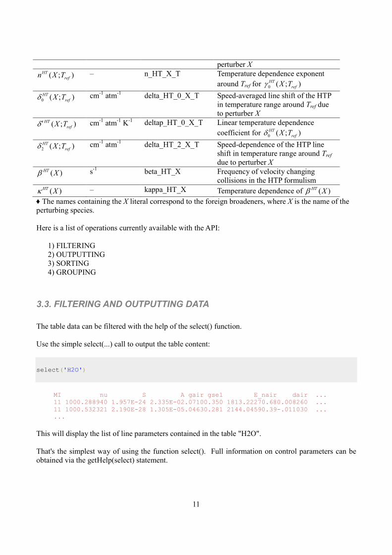
Use the simple select(...) call to output the table content:

select('H2O')

MI nu S A gair gsel E_nair dair ... 11 1000.288940 1.957E-24 2.335E-02.07100.350 1813.22270.680.008260 ... 11 1000.532321 2.190E-28 1.305E-05.04630.281 2144.04590.39-.011030 ... ...

This will display the list of line parameters contained in the table "H2O".

That's the simplest way of using the function select(). Full information on control parameters can be

obtained via the getHelp(select) statement.

12

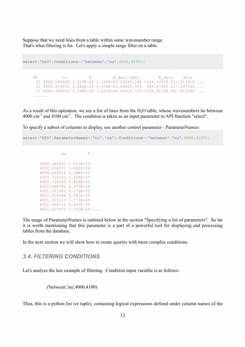
Suppose that we need lines from a table within some wavenumber range.

That's what filtering is for. Let's apply a simple range filter on a table.

select('H2O',Conditions=('between','nu',4000,4100))

MI nu S A gair gsel E_nair dair 11 4000.188800 1.513E-25 1.105E-02.03340.298 1581.33570.51-.013910 ... 11 4000.204070 3.482E-24 8.479E-03.08600.454 586.47920.61-.007000 ... 11 4000.469910 3.268E-23 1.627E+00.05410.375 1255.91150.56-.013050 ... ......

As a result of this operation, we see a list of lines from the H2O table, whose wavenumbers lie between

4000 cm-1

and 4100 cm-1

. The condition is taken as an input parameter to API function "select".

To specify a subset of columns to display, use another control parameter - ParameterNames:

select('H2O',ParameterNames=('nu','sw'),Conditions=('between','nu',4000,4100))

nu S

4000.188800 1.513E-25 4000.204070 3.482E-24 4000.469910 3.268E-23 4000.722241 1.528E-27 4000.730660 5.406E-25 4000.999780 6.975E-29 4001.281900 9.279E-23 4001.319998 2.591E-29 4001.323119 7.773E-29 4001.325110 2.997E-25 4001.427670 1.791E-24 ...

The usage of ParameterNames is outlined below in the section "Specifying a list of parameters". So far

it is worth mentioning that this parameter is a part of a powerful tool for displaying and processing

tables from the database.

In the next section we will show how to create queries with more complex conditions.

3.4. FILTERING CONDITIONS

Let's analyze the last example of filtering. Condition input variable is as follows:

('between','nu',4000,4100)

Thus, this is a python list (or tuple), containing logical expressions defined under column names of the

13

table. For example, 'nu' is a name of the column in 'H2O' table, and this column contains a transition

wavenumber.

The structure of a simple condition is as follows:

(OPERATION,ARG1,ARG2,...)

where OPERATION must be in a set of predefined operations (see below), and ARG1,ARG2, etc. are

the arguments for this operation.

Conditions can be nested, i.e. ARG can itself be a condition (see examples).

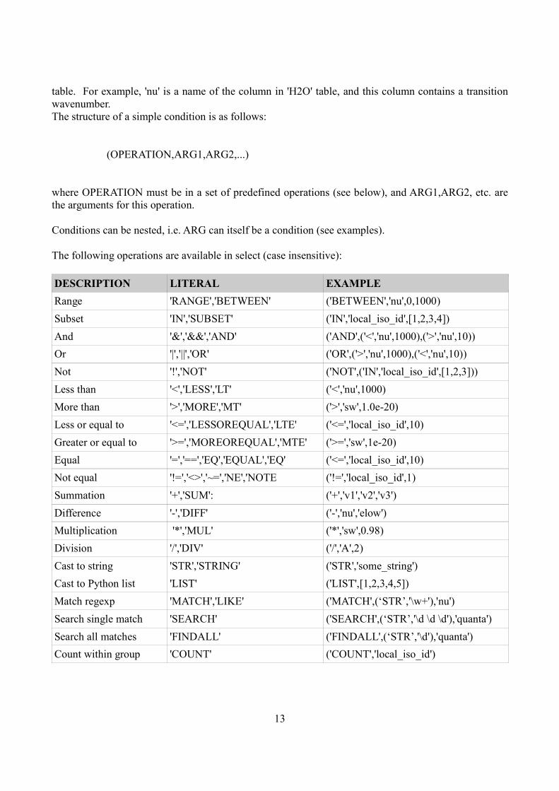
The following operations are available in select (case insensitive):

DESCRIPTION LITERAL EXAMPLE

Range 'RANGE','BETWEEN' ('BETWEEN','nu',0,1000)

Subset 'IN','SUBSET' ('IN','local_iso_id',[1,2,3,4])

And '&','&&','AND' ('AND',('<','nu',1000),('>','nu',10))

Or '|','||','OR' ('OR',('>','nu',1000),('<','nu',10))

Not '!','NOT' ('NOT',('IN','local_iso_id',[1,2,3]))

Less than '<','LESS','LT' ('<','nu',1000)

More than '>','MORE','MT' ('>','sw',1.0e-20)

Less or equal to '<=','LESSOREQUAL','LTE' ('<=','local_iso_id',10)

Greater or equal to '>=','MOREOREQUAL','MTE' ('>=','sw',1e-20)

Equal '=','==','EQ','EQUAL','EQ' ('<=','local_iso_id',10)

Not equal '!=','<>','~=','NE','NOTE ('!=','local_iso_id',1)

Summation '+','SUM': ('+','v1','v2','v3')

Difference '-','DIFF' ('-','nu','elow')

Multiplication '*','MUL' ('*','sw',0.98)

Division '/','DIV' ('/','A',2)

Cast to string 'STR','STRING' ('STR','some_string')

Cast to Python list 'LIST' ('LIST',[1,2,3,4,5])

Match regexp 'MATCH','LIKE' ('MATCH',(‘STR’,'\w+'),'nu')

Search single match 'SEARCH' ('SEARCH',(‘STR’,'\d \d \d'),'quanta')

Search all matches 'FINDALL' ('FINDALL',(‘STR’,'\d'),'quanta')

Count within group 'COUNT' ('COUNT','local_iso_id')

14

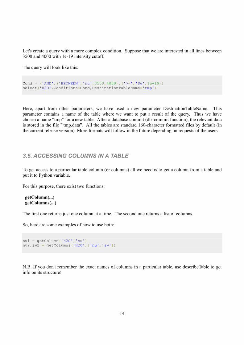
Let's create a query with a more complex condition. Suppose that we are interested in all lines between

3500 and 4000 with 1e-19 intensity cutoff.

The query will look like this:

Cond = ('AND',('BETWEEN','nu',3500,4000),('>=','Sw',1e-19)) select('H2O',Conditions=Cond,DestinationTableName='tmp')

Here, apart from other parameters, we have used a new parameter DestinationTableName. This

parameter contains a name of the table where we want to put a result of the query. Thus we have

chosen a name “tmp” for a new table. After a database commit (db_commit function), the relevant data

is stored in the file '”tmp.data”. All the tables are standard 160-character formatted files by default (in

the current release version). More formats will follow in the future depending on requests of the users.

3.5. ACCESSING COLUMNS IN A TABLE

To get access to a particular table column (or columns) all we need is to get a column from a table and

put it to Python variable.

For this purpose, there exist two functions:

getColumn(...)

getColumns(...)

The first one returns just one column at a time. The second one returns a list of columns.

So, here are some examples of how to use both:

nu1 = getColumn('H2O','nu') nu2,sw2 = getColumns('H2O',['nu','sw'])

N.B. If you don't remember the exact names of columns in a particular table, use describeTable to get

info on its structure!

15

3.6. SPECIFYING A LIST OF PARAMETERS

Suppose that we want not only to select a set of parameters/columns from a table, but to perform

certain transformations on them (for example, multiply a column by a coefficient, or add one column to

another etc...).

We can do it in two ways. First, we can extract a column from the table using one of the functions

(getColumn or getColumns) and do the rest in Python. The second way is to do it on the level of select.

The select function has a control parameter "ParameterNames", which makes it possible to specify

parameters we want to be selected, and perform some simple arithmetic expressions with them.

Assume that we need only wavenumber and intensity from the H2O table.

Also we need to scale the intensity to unitary abundance. To do so, we must divide an 'sw' parameter

by its natural abundance (0.99731 for the principal isotopologue of water).

Thus, we have to select two columns: wavenumber (nu) and scaled intensity (sw/0.99731)

select('H2O',ParameterNames=('nu',('/','sw',0.99731)))

nu #0 3400.006750 1.116002045502401E-23 3400.335198 6.218728379340426E-28 3400.397711 4.341679116824257E-27 3400.405850 1.298492946024807E-24 3400.445191 2.045502401459927E-27 3400.550910 6.715063520871143E-26 3400.566080 4.490078310655663E-24 3400.581360 2.010407997513311E-25 ...

3.7. SAVING QUERY TO DISK

To quickly save a result of a query to disk, the user can take advantage of an additional parameter

"File". If this parameter is presented in the function call, then the query is saved to a file with the name

which was specified in "File".

For example, select all lines from H2O and save the result in file 'H2O.txt':

select('H2O',File='H2O.txt')

16

3.8. GETTING INFORMATION ON ISOTOPOLOGUES

HAPI provides the following auxiliary information about isotopologues present in HITRAN.

Corresponding functions use the standard HITRAN molecule-isotopologue notation:

1) Natural abundances

abundance(mol_id,iso_id)

2) Molecular masses

molecularMass(mol_id,iso_id)

3) Molecule names

moleculeName(mol_id,iso_id)

4) Isotopologue names

isotopologueName(mol_id,iso_id)

5) ISO_ID

getHelp(ISO_ID)

The latter is a dictionary, which contains the summary information about all isotopologues available in

HAPI.

17

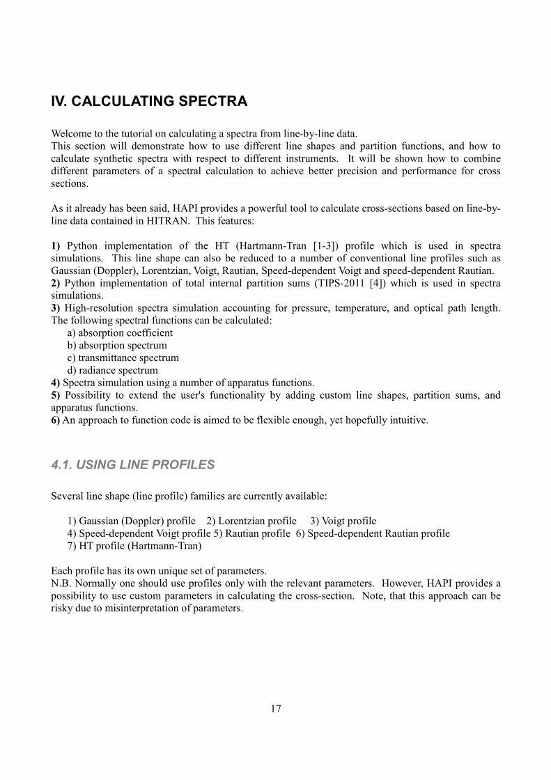
IV. CALCULATING SPECTRA

Welcome to the tutorial on calculating a spectra from line-by-line data.

This section will demonstrate how to use different line shapes and partition functions, and how to

calculate synthetic spectra with respect to different instruments. It will be shown how to combine

different parameters of a spectral calculation to achieve better precision and performance for cross

sections.

As it already has been said, HAPI provides a powerful tool to calculate cross-sections based on line-by-

line data contained in HITRAN. This features:

1) Python implementation of the HT (Hartmann-Tran [1-3]) profile which is used in spectra

simulations. This line shape can also be reduced to a number of conventional line profiles such as

Gaussian (Doppler), Lorentzian, Voigt, Rautian, Speed-dependent Voigt and speed-dependent Rautian.

2) Python implementation of total internal partition sums (TIPS-2011 [4]) which is used in spectra

simulations.

3) High-resolution spectra simulation accounting for pressure, temperature, and optical path length.

The following spectral functions can be calculated:

a) absorption coefficient

b) absorption spectrum

c) transmittance spectrum

d) radiance spectrum

4) Spectra simulation using a number of apparatus functions.

5) Possibility to extend the user's functionality by adding custom line shapes, partition sums, and

apparatus functions.

6) An approach to function code is aimed to be flexible enough, yet hopefully intuitive.

4.1. USING LINE PROFILES

Several line shape (line profile) families are currently available:

1) Gaussian (Doppler) profile 2) Lorentzian profile 3) Voigt profile

4) Speed-dependent Voigt profile 5) Rautian profile 6) Speed-dependent Rautian profile

7) HT profile (Hartmann-Tran)

Each profile has its own unique set of parameters.

N.B. Normally one should use profiles only with the relevant parameters. However, HAPI provides a

possibility to use custom parameters in calculating the cross-section. Note, that this approach can be

risky due to misinterpretation of parameters.

18

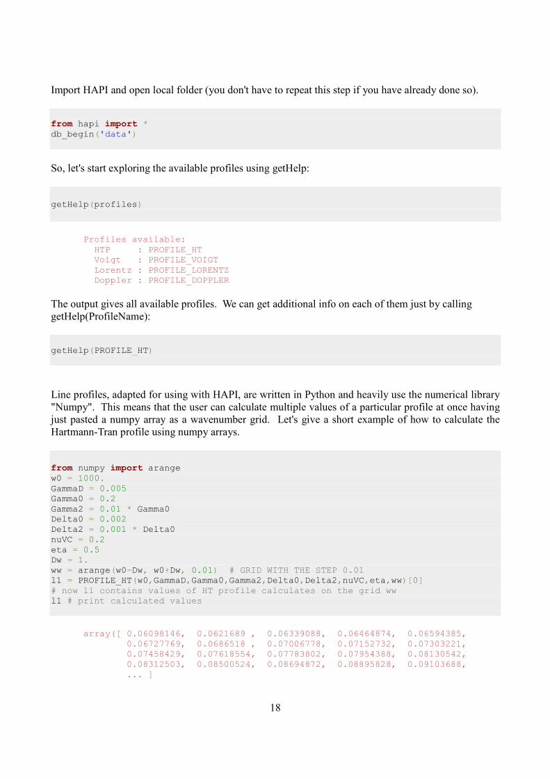
Import HAPI and open local folder (you don't have to repeat this step if you have already done so).

from hapi import * db_begin('data')

So, let's start exploring the available profiles using getHelp:

getHelp(profiles)

Profiles available: HTP : PROFILE_HT Voigt : PROFILE_VOIGT Lorentz : PROFILE_LORENTZ Doppler : PROFILE_DOPPLER

The output gives all available profiles. We can get additional info on each of them just by calling

getHelp(ProfileName):

getHelp(PROFILE_HT)

Line profiles, adapted for using with HAPI, are written in Python and heavily use the numerical library

"Numpy". This means that the user can calculate multiple values of a particular profile at once having

just pasted a numpy array as a wavenumber grid. Let's give a short example of how to calculate the

Hartmann-Tran profile using numpy arrays.

from numpy import arange w0 = 1000. GammaD = 0.005 Gamma0 = 0.2 Gamma2 = 0.01 * Gamma0 Delta0 = 0.002 Delta2 = 0.001 * Delta0 nuVC = 0.2 eta = 0.5 Dw = 1. ww = arange(w0-Dw, w0+Dw, 0.01) # GRID WITH THE STEP 0.01 l1 = PROFILE_HT(w0,GammaD,Gamma0,Gamma2,Delta0,Delta2,nuVC,eta,ww)[0] # now l1 contains values of HT profile calculates on the grid ww l1 # print calculated values

array([ 0.06098146, 0.0621689 , 0.06339088, 0.06464874, 0.06594385, 0.06727769, 0.0686518 , 0.07006778, 0.07152732, 0.07303221, 0.07458429, 0.07618554, 0.07783802, 0.07954388, 0.08130542, 0.08312503, 0.08500524, 0.08694872, 0.08895828, 0.09103688, ... ]

19

For additional information about parameters see getHelp(PROFILE_HT).

It is worth noting that PROFILE_HT returns 2 entities: the real and imaginary part of the line shape (as

is described in Ref. [1]). Apart from HT, all other profiles return just one entity (the real part).

4.2. USING PARTITION SUMS

As mentioned in Section 4.1, the partition sums are taken from the TIPS-2011 [4]. Partition sums are

taken for those isotopologues which are present in HITRAN and in TIPS-2011 simultaneously.

N.B. Partition sums are not yet available for the following isotopologues which are in HITRAN at the

current time:

Isotopologue ID Molecule number Isotopologue number Isotopologue name

117 12 2 H15

N16

O3

110 14 2 D19F

107 15 3 D35

Cl

108 15 4 D37

Cl

111 16 3 D79

Br

112 16 4 D81

Br

113 17 2 D127

I

118 22 2 14

N15

N

119 29 2 13C16O19F2

86 34 1 16

O

92 39 1 12

CH316

OH

114 47 1 32

S16

O3

The data on these isotopologues are not present in TIPS-2011 but the isotopologues are present in

HITRAN. We're planning to add these molecules after a new TIPS program is released.

To calculate a partition sum for most of the isotopologues in HITRAN, we will use a function

partitionSum (use getHelp for detailed info).

The syntax is as follows: partitionSum(M,I,T), where M,I - standard HITRAN molecule-isotopologue

notation, T - definition of temperature range.

20

Usecase 1: temperature is defined by a list: Q = partitionSum(1,1,[70,80,90]) Q

[20.999999542236328, 25.446399765014647, 30.169152160644533]

Usecase 2: temperature is defined by bounds and the step:

T,Q = partitionSum(1,1,[70,3000],step=1.0) Q

array([ 20.99999954, 21.43247156, 21.86764758, ..., 15942.1616 , 15957.8416 , 15973.5344 ])

In the latter example, we calculate a partition sum on a range of temperatures from 70K to 3000K using

a step 1.0 K, and having arrays of temperature (T) and partition sum (Q) as the output.

4.3. CALCULATING ABSORPTION COEFFICIENTS

Currently HAPI can calculate the following spectral function at arbitrary thermodynamic parameters:

1) Absorption coefficient

2) Absorption spectrum

3) Transmittance spectrum

4) Radiance spectrum

All these functions can be calculated with or without accounting of instrument properties (apparatus

function, resolution, path length etc...)

As is well known, the spectral functions such as absorption, transmittance, and radiance, are calculated

on the basis of the absorption coefficient. For that reason, absorption coefficient is the most important

part of simulating a cross section. This part of the tutorial is devoted to a demonstration of how to

calculate the absorption coefficient from the HITRAN line-by-line data. Here we give a brief insight

on basic parameters of the calculation procedure, and talk about some useful practices and precautions.

21

To calculate an absorption coefficient, we can use one of the following functions:

-> absorptionCoefficient_HT

-> absorptionCoefficient_Voigt

-> absorptionCoefficient_Lorentz

-> absorptionCoefficient_Doppler

-> absorptionCoefficient_SDVoigt

-> absorptionCoefficient_Galatry

Each of these functions calculates cross sections using different line shapes (the names are quite self-

explanatory).

You can get detailed information on using each of these functions by calling getHelp(function_name).

___________________________________________________________________________________

Let's look more closely to the cross sections based on the Lorentz profile. For doing that, let's have a

table downloaded from HITRANonline.

Get data on CO2 main isotopologue in the range 2000-2100 cm-1:

fetch('CO2',2,1,2000,2100)

OK, now we're ready to run a fast example of how to calculate an absorption coefficient cross section:

nu,coef = absorptionCoefficient_Lorentz(SourceTables='CO2')

This example calculates a Lorentz cross section using the whole set of lines in the "CO2" table. This is

the simplest possible way to use these functions, because the major part of parameters are constrained

to their default values.

22

If we have Matplotlib installed, then we can visualize it using a plotter:

from pylab import plot plot(nu,coef)

More examples on how to use Matplotlib can be found in the Section V. Plotting with Matplotlib.

23

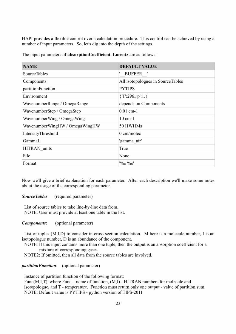
HAPI provides a flexible control over a calculation procedure. This control can be achieved by using a

number of input parameters. So, let's dig into the depth of the settings.

The input parameters of absorptionCoefficient_Lorentz are as follows:

NAME DEFAULT VALUE

SourceTables '__BUFFER__'

Components All isotopologues in SourceTables

partitionFunction PYTIPS

Environment {'T':296.,'p':1.}

WavenumberRange / OmegaRange depends on Components

WavenumberStep / OmegaStep 0.01 cm-1

WavenumberWing / OmegaWing 10 cm-1

WavenumberWingHW / OmegaWingHW 50 HWHMs

IntensityThreshold 0 cm/molec

GammaL 'gamma_air'

HITRAN_units True

File None

Format '%e %e'

Now we'll give a brief explanation for each parameter. After each description we'll make some notes

about the usage of the corresponding parameter.

SourceTables: (required parameter)

List of source tables to take line-by-line data from.

NOTE: User must provide at least one table in the list.

Components: (optional parameter)

List of tuples (M,I,D) to consider in cross section calculation. M here is a molecule number, I is an

isotopologue number, D is an abundance of the component.

NOTE: If this input contains more than one tuple, then the output is an absorption coefficient for a

mixture of corresponding gases.

NOTE2: If omitted, then all data from the source tables are involved.

partitionFunction: (optional parameter)

Instance of partition function of the following format:

Func(M,I,T), where Func – name of function, (M,I) - HITRAN numbers for molecule and

isotopologue, and T - temperature. Function must return only one output - value of partition sum.

NOTE: Default value is PYTIPS - python version of TIPS-2011

24

Environment: (optional parameter)

Python dictionary containing value of pressure and temperature.

The format is as follows: Environment = {'p':pval,'T':tval}, where "pval" and "tval" are corresponding

values in atm and K respectively.

NOTE: Default value is {'p':1.0,'T':296.0}

WavenumberRange / OmegaRange: (optional parameter)

List containing minimum and maximum value of wavenumber to consider in cross-section

calculation. All lines that are out of these bounds will be skipped.

The format is as follows: OmegaRange=[wn_low,wn_high]

NOTE: If this parameter is skipped, then min and max are taken from the data in SourceTables.

WavenumberStep / OmegaStep: (optional parameter)

Value for the wavenumber step.

NOTE: Default value is 0.01 cm-1

.

NOTE2: Normally the user would want to take the step under 0.001 when calculating absorption

coefficient with Doppler profile because of very narrow spectral lines.

WavenumberWing / OmegaWing: (optional parameter)

Absolute value of the line wing in cm-1, i.e. distance from the center of each line to the farthest point

where the profile is considered to be non zero.

NOTE: if omitted, then only OmegaWingHW is taken into account.

WavenumberWingHW / OmegaWingHW: (optional parameter)

Relative value of the line wing in halfwidths.

NOTE: The resulting wing is a maximum value from both OmegaWing and

OmegaWingHW.

IntensityThreshold: (optional parameter)

Absolute value of minimum intensity in cm-1

/ (molec × cm-2

) to consider2.

NOTE: default value is 0.

NOTE2: Setting this parameter to a value above zero is only recommended for very experienced

users.

GammaL: (optional parameter)

This is the name of broadening parameter to consider a "Lorentzian" part in the Voigt profile. In the

current 160-character format there is a choice between "gamma_air" and "gamma_self".

NOTE: If the table has custom columns with broadening coefficients, the user can specify the name of

this column in GammaL. This would let the function calculate an absorption with custom

broadening parameter.

2 In this manual this unit could be also be expressed as cm / molec

25

HITRAN_units: (optional parameter)

Logical flag for units in which the absorption coefficient should be calculated. Currently, the choices

are: cm^2/molec (if True) and cm-1 (if False).

NOTE: to calculate other spectral functions like transmittance, radiance and absorption spectra, the

user should set HITRAN_units to False.

File: (optional parameter)

The name of the file to save the calculated absorption coefficient. The file is saved only if this

parameter is specified.

Format: (optional parameter)

C-style format for the text data to be saved. Default value is "%e %e".

NOTE: C-style output format specification (which is mostly valid for Python) can be found, for

instance, by the link: http://www.gnu.org/software/libc/manual/html_node/Formatted-Output.html

WavenumberGrid / OmegaGrid (optional parameter)

An array or list representing a user’s custom grid to calculate cross-section.

NOTE: Default value is None

NOTE2: If specified, OmegaGrid discards OmegaRange and OmegaStep

NOTE3: If omitted, OmegaRange and OmegaStep are used to define the grid.

N.B. Other functions such as absorptionCoefficient_Voigt(_HT,_Doppler) have identical parameter sets

so the description is the same for each function.

4.4. CALCULATING ABSORPTION, TRANSMITTANCE, AND RADIANCE SPECTRA

Let's calculate an absorption, transmittance, and radiance spectra on the basis of absorption coefficient.

In order to be consistent with internal API's units, we need to have an absorption coefficient in cm-1

:

nu,coef = absorptionCoefficient_Lorentz(SourceTables='CO2',HITRAN_units=False)

To calculate absorption spectrum, use the function absorptionSpectrum():

nu,absorp = absorptionSpectrum(nu,coef)

To calculate transmittance spectrum, use function transmittanceSpectrum():

nu,trans = transmittanceSpectrum(nu,coef)

26

To calculate radiance spectrum, use function radianceSpectrum():

nu,radi = radianceSpectrum(nu,coef)

The last three commands used a default path length (1 m). To see complete info on all three functions,

look for the section "calculating spectra" in getHelp()

Generally, all these three functions use a similar set of parameters:

Wavenumber / Omegas: (required parameter)

Wavenumber grid for spectrum.

AbsorptionCoefficient: (optional parameter)

Absorption coefficient as input.

Environment: (optional parameter)

Environmental parameters for calculating spectrum. This parameter is a bit specific for each of the

functions. For absorptionSpectrum(...) and transmittanceSpectrum(...) the default value is as follows:

Environment={'l': 100.0}. For transmittanceSpectrum() the default value, besides path length,

contains a temperature: Environment={'T': 296.0, 'l': 100.0}

NOTE: temperature must be equal to that which was used in the absorptionCoefficient_(...) routine!

File: (optional parameter)

Filename of output file for calculated spectrum. If omitted, then the file is not created.

Format: (optional parameter)

C-style format for spectra output file.

NOTE: Default value is as follows: Format='%e %e'

4.5. APPLYING INSTRUMENTAL FUNCTIONS

For comparison of the theoretical spectra with the real-world instrument output, it's necessary to take

into account instrumental resolution. For this purpose, HAPI has a function convolveSpectrum(...)

which can calculate spectra with variable resolution using custom instrumental functions.

The following instrumental functions are available:

1) Rectangular (Boxcar) 2) Triangular 3) Gaussian

4) Dispersion (Lorentz) 5) Diffraction 6) Michelson

27

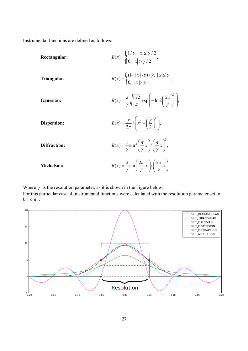
Instrumental functions are defined as follows:

Rectangular: 1/ , / 2

( )0, / 2

xB x

x

γ γ

γ

≤=

>,

Triangular: (1 | | / ) / , | |

( )0, | |

x xB x

x

γ γ γγ

− ≤=

>,

Gaussian:

2

2 ln 2 2( ) exp ln 2

xB x

γ π γ

= −

,

Dispersion:

2

2( ) /2 2

B x xγ γπ

= + ,

Diffraction:

2

21( ) sin /B x x x

π πγ γ γ

=

,

Michelson: 2 2 2

( ) sin /B x x xπ π

γ γ γ

=

Where γ is the resolution parameter, as it is shown in the Figure below.

For this particular case all instrumental functions were calculated with the resolution parameter set to

0.1 cm-1

.

28

To get a description of each instrumental function one can use getHelp():

getHelp(slit_functions)

RECTANGULAR : SLIT_RECTANGULAR TRIANGULAR : SLIT_TRIANGULAR GAUSSIAN : SLIT_GAUSSIAN DIFFRACTION : SLIT_DIFFRACTION MICHELSON : SLIT_MICHELSON DISPERSION/LORENTZ : SLIT_DISPERSION

For instance,

getHelp(SLIT_MICHELSON)

... will give detailed info about the Michelson instrumental function.

The function convolveSpectrum() convolves a high-resolution spectrum with one of the supplied

instrumental (slit) functions. The following parameters of this function are provided:

Wavenumber / Omega: (required parameter)

Array of wavenumbers in high-resolution input spectrum.

CrossSection: (required parameter)

Values of high-resolution input spectrum.

Resolution: (optional parameter)

This parameter is passed to the slit function. It represents the resolution of the corresponding

instrument.

NOTE: default value is 0.1 cm-1

AF_wing: (optional parameter)

Width of an instrument function where it is considered non-zero.

NOTE: default value is 10.0 cm-1

SlitFunction: (optional parameter)

Custom instrumental function to convolve with spectrum. Format of the instrumental function must

be

as follows: Func(x,g), where Func - function name, x - wavenumber, g - resolution.

NOTE: if omitted, then the default value is SLIT_RECTANGULAR

29

Before using the convolution procedure it is worth giving some practical advice and remarks:

1) The quality of a convolution depends of many things: quality of calculated spectra, width of

AF_wing and OmegaRange, Resolution, OmegaStep etc… Most of these factors are taken from

previous stages of the spectral calculation. The right choice of all these factors is crucial for the correct

computation.

2) Dispersion, Diffraction and Michelson apparatus functions don't work well in a narrow wavenumber

range because of their broad wings.

3) Generally one must consider OmegaRange and AF_wing as wide as possible.

4) After applying a convolution, the resulting spectral range for the convolved spectra is reduced by the

doubled value of AF_wing. For this reason, try to make an initial spectral range for high-resolution

spectrum (absorption, transmittance, radiance) sufficiently broad.

5) convolveSpectrum can be easily used with external data since it does not depend on database tables

The following command will calculate a convolved spectra from the CO2 transmittance, which was

calculated in a previous section.

The spectral resolution is 0.1 cm-1

by default.

nu_,trans_,i1,i2,slit = convolveSpectrum(nu,trans)

The outputs in this case are:

nu_, trans_ – wavenumbers and transmittance for the resulting convolved spectrum.

i1,i2 – indexes for initial nu,trans spectrum denoting the part of wavenumber range which was taken for

convolved spectrum. Thus, the resulting spectrum is calculated on nu[i1:i2]

slit – array of slit function values calculated on grid “nu”

Note, in order to achieve more flexibility, one has to specify most of the optional parameters. For

instance, a more complete call is as follows:

nu_,trans_,i1,i2,slit = convolveSpectrum(nu,trans,SlitFunction=SLIT_MICHELSON,Resolution=1.0,AF_wing=20.0)

4.6. ALIASES

To simplify the usage of HAPI, aliases (i.e. shortcuts) are given for the cross section functions:

abscoef_HT => absorptionCoefficient_HT

abscoef_Voigt => absorptionCoefficient_Voigt

abscoef_Lorentz => absorptionCoefficient_Lorentz

abscoef_Doppler => absorptionCoefficient_Doppler

abscoef_Gauss => absorptionCoefficient_Doppler

30

The correspondence between the alias and the full function is as follows:

abscoef_Prof(table,step,grid,env,file) ======>

absorptionCoefficient_Prof(SourceTables=table,OmegaStep=step,

OmegaGrid=grid,Environment=env,File=file),

where Prof is the profile name (HT, Voigt, Lorentz, Doppler)

The default values of parameters are the same for each type of function given:

table=None, step=None, grid=None, env={'T':296.,'p':1.}, file=None

NOTE: In aliases both function and parameter names are shortened.

NOTE2: One can use full versions of each function to be able to tweak all available parameters.

NOTE3: It is possible to create your own aliases using the same approach as shown in this subsection.

31

V. PLOTTING WITH MATPLOTLIB

This section briefly explains how to make plots using the Matplotlib - Python library for plotting.

Let's generate a plot using the basic entities which are provided by HAPI.

To do so, we will do all necessary steps to download, filter and calculate cross sections "from scratch".

To demonstrate the different possibilities of matplotlib, we will mostly use Pylab - a part of Matplotlib

with an interface similar to Matlab. Please note that it's not the only way to use Matplotlib. More

information can be found on its site.

The next part is a step-by-step guide, demonstrating basic possibilities of HAPI in conjunction with

Matplotlib.

First, do some preliminary imports:

from hapi import * from pylab import show,plot,subplot,xlim,ylim,title,legend,xlabel,ylabel,hold

Start the local database in folder 'data':

db_begin('data')

Download lines for the main isotopologue of ozone in the [3900,4050] range:

fetch('O3',3,1,3900,4050)

32

Plot a stick spectrum using the function getStickXY(...):

x,y = getStickXY('O3') plot(x,y); show()

33

Zoom in spectral region [4020,4035] cm-1:

plot(x,y,'.'); xlim([4020,4035]); show()

34

Calculate and plot difference between Voigt and Lorentzian lineshape:

wn = arange(3002,3008,0.01) # get wavenumber range of interest voi = PROFILE_VOIGT(3005,0.1,0.3,wn)[0] # calc Voigt lor = PROFILE_LORENTZ(3005,0.3,wn) # calc Lorentz diff = voi-lor # calc difference subplot(2,1,1) # upper panel plot(wn,voi,'red',wn,lor,'blue') # plot both profiles legend(['Voigt','Lorentz']) # show legend title('Voigt and Lorentz profiles') # show title subplot(2,1,2) # lower panel plot(wn,diff) # plot difference title('Voigt-Lorentz residual') # show title show() # show all figures

35

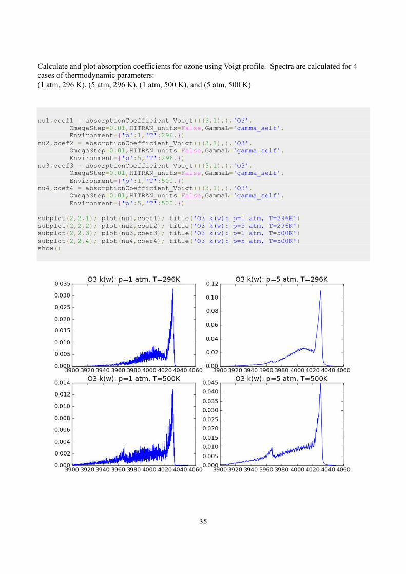
Calculate and plot absorption coefficients for ozone using Voigt profile. Spectra are calculated for 4

cases of thermodynamic parameters:

(1 atm, 296 K), (5 atm, 296 K), (1 atm, 500 K), and (5 atm, 500 K)

nu1,coef1 = absorptionCoefficient_Voigt(((3,1),),'O3', OmegaStep=0.01,HITRAN_units=False,GammaL='gamma_self', Environment={'p':1,'T':296.}) nu2,coef2 = absorptionCoefficient_Voigt(((3,1),),'O3', OmegaStep=0.01,HITRAN_units=False,GammaL='gamma_self', Environment={'p':5,'T':296.}) nu3,coef3 = absorptionCoefficient_Voigt(((3,1),),'O3', OmegaStep=0.01,HITRAN_units=False,GammaL='gamma_self', Environment={'p':1,'T':500.}) nu4,coef4 = absorptionCoefficient_Voigt(((3,1),),'O3', OmegaStep=0.01,HITRAN_units=False,GammaL='gamma_self', Environment={'p':5,'T':500.}) subplot(2,2,1); plot(nu1,coef1); title('O3 k(w): p=1 atm, T=296K') subplot(2,2,2); plot(nu2,coef2); title('O3 k(w): p=5 atm, T=296K') subplot(2,2,3); plot(nu3,coef3); title('O3 k(w): p=1 atm, T=500K') subplot(2,2,4); plot(nu4,coef4); title('O3 k(w): p=5 atm, T=500K') show()

36

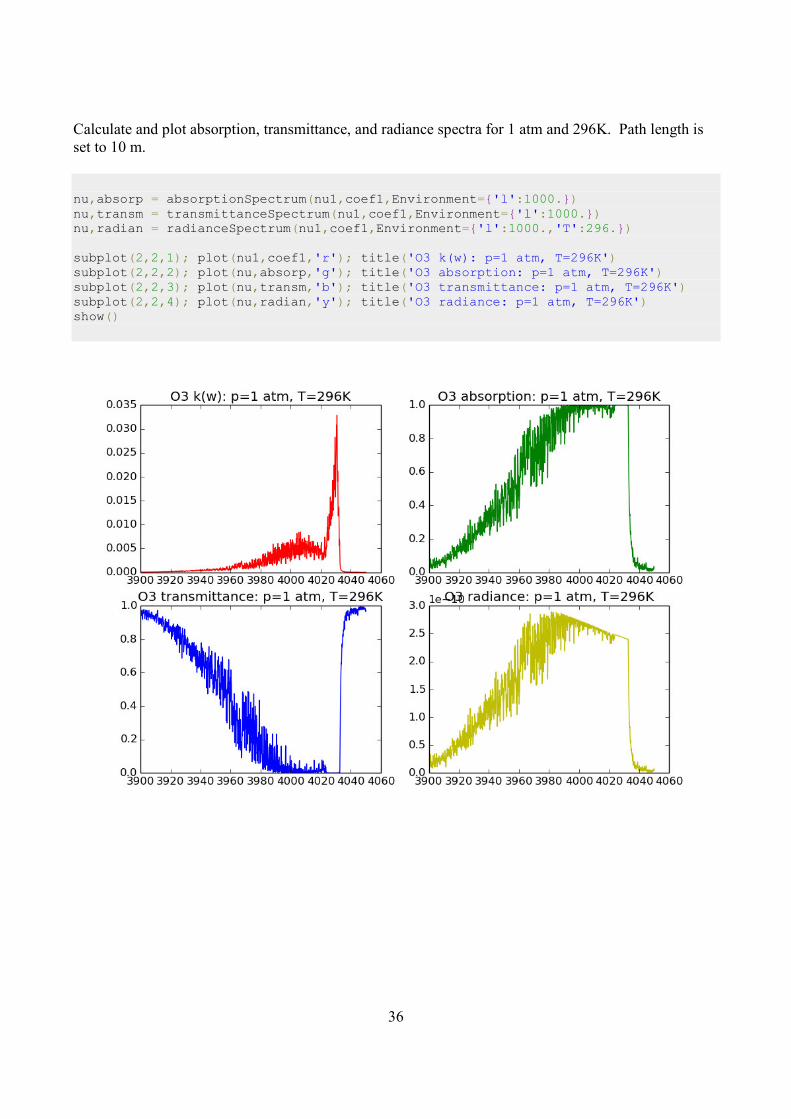
Calculate and plot absorption, transmittance, and radiance spectra for 1 atm and 296K. Path length is

set to 10 m.

nu,absorp = absorptionSpectrum(nu1,coef1,Environment={'l':1000.}) nu,transm = transmittanceSpectrum(nu1,coef1,Environment={'l':1000.}) nu,radian = radianceSpectrum(nu1,coef1,Environment={'l':1000.,'T':296.}) subplot(2,2,1); plot(nu1,coef1,'r'); title('O3 k(w): p=1 atm, T=296K') subplot(2,2,2); plot(nu,absorp,'g'); title('O3 absorption: p=1 atm, T=296K') subplot(2,2,3); plot(nu,transm,'b'); title('O3 transmittance: p=1 atm, T=296K') subplot(2,2,4); plot(nu,radian,'y'); title('O3 radiance: p=1 atm, T=296K') show()

37

Calculate and compare high-resolution spectrum for O3 with lower resolution spectrum convoluted

with an instrumental function of an ideal Michelson interferometer.

nu_,trans_,i1,i2,slit = convolveSpectrum(nu,transm,SlitFunction=SLIT_MICHELSON, Resolution=1.0,AF_wing=20.0) plot(nu,transm,'red',nu_,trans_,'blue'); legend(['HI-RES','Michelson']); show()

38

VI. KEY FUNCTIONS: EXAMPLES

6.1. Help system

HAPI has an interactive help system which is provided by the function getHelp().

To get an access to it, run getHelp() in your console and it will give options which you can provide to

getHelp() as in input:

getHelp()

For example, getHelp(tutorials) provides tutorials on data filtering, spectra calculation, Python

language etc…

getHelp(tutorials)

Calling getHelp(name_of_the_function) gives separate help on each principal function of HAPI:

getHelp(PROFILE_HT)

The next sub-sections contain document strings for each principal function of HAPI.

6.2. Fetching data

__________________________________________________________________________________

fetch(TableName, M, I, numin, numax)

INPUT PARAMETERS: TableName: local table name to fetch in (required) M: HITRAN molecule number (required) I: HITRAN isotopologue number (required) numin: lower wavenumber bound (required) numax: upper wavenumber bound (required) OUTPUT PARAMETERS: none --- DESCRIPTION: Download line-by-line data from HITRANonline server and save it to local table. The input parameters M and I are the HITRAN molecule and isotopologue numbers. This function results in a table containing single isotopologue specie. To have multiple species in a

39

single table use fetch_by_ids instead. --- EXAMPLE OF USAGE: fetch('HOH',1,1,4000,4100) ---

__________________________________________________________________________________

fetch_by_ids(TableName, iso_id_list, numin, numax) INPUT PARAMETERS: TableName: local table name to fetch in (required) iso_id_list: list of isotopologue id's (required) numin: lower wavenumber bound (required) numax: upper wavenumber bound (required) OUTPUT PARAMETERS: none --- DESCRIPTION: Download line-by-line data from HITRANonline server and save it to local table. The input parameter iso_id_list contains list of "global" isotopologue Ids (see help on ISO_ID). Note: this function is required if user wants to download multiple species into single table. --- EXAMPLE OF USAGE: fetch_by_ids('water',[1,2,3,4],4000,4100)

__________________________________________________________________________________

6.3. Working with data

__________________________________________________________________________________

db_begin(db=None) INPUT PARAMETERS: db: database name (optional) OUTPUT PARAMETERS: none --- DESCRIPTION: Open a database connection. A database is stored in a folder given in db input parameter. Default=data --- EXAMPLE OF USAGE: db_begin('bar') ---

__________________________________________________________________________________

db_commit() INPUT PARAMETERS: none OUTPUT PARAMETERS: none

40

--- DESCRIPTION: Commit all changes made to opened database. All tables will be saved in corresponding files. --- EXAMPLE OF USAGE: db_commit() ---

__________________________________________________________________________________

tableList() INPUT PARAMETERS: none OUTPUT PARAMETERS: TableList: a list of available tables --- DESCRIPTION: Return a list of tables present in database. --- EXAMPLE OF USAGE: lst = tableList() ---

__________________________________________________________________________________

describeTable(TableName) INPUT PARAMETERS: TableName: name of the table to describe OUTPUT PARAMETERS: none --- DESCRIPTION: Print information about table, including parameter names, formats and wavenumber range. --- EXAMPLE OF USAGE: describe('sampletab') ---

__________________________________________________________________________________

select(TableName, DestinationTableName='__BUFFER__', ParameterNames=None, Conditions=None, Output=True, File=None) INPUT PARAMETERS: TableName: name of source table (required) DestinationTableName: name of resulting table (optional) ParameterNames: list of parameters or expressions (optional) Conditions: list of logical expressions (optional) Output: enable (True) or suppress (False) text output (optional) File: enable (True) or suppress (False) file output (optional) OUTPUT PARAMETERS: none --- DESCRIPTION: Select or filter the data in some table either to standard output or to file (if specified) --- EXAMPLE OF USAGE: select('sampletab',DestinationTableName='outtab',ParameterNames=(p1,p2),

41

Conditions=(('and',('>=','p1',1),('<',('*','p1','p2'),20)))) Conditions means (p1>=1 and p1*p2<20) ---

__________________________________________________________________________________

sort(TableName, DestinationTableName=None, ParameterNames=None, Accending=True, Output=False, File=None) INPUT PARAMETERS: TableName: name of source table (required) DestinationTableName: name of resulting table (optional) ParameterNames: list of parameters or expressions to sort by (optional) Accending: sort in ascending (True) or descending (False) order (optional) Output: enable (True) or suppress (False) text output (optional) File: enable (True) or suppress (False) file output (optional) OUTPUT PARAMETERS: none --- DESCRIPTION: Sort a table by a list of its parameters or expressions. The sorted table is saved in DestinationTableName (if specified). --- EXAMPLE OF USAGE: sort('sampletab',ParameterNames=(p1,('+','p1','p2'))) ---

__________________________________________________________________________________

group(TableName, DestinationTableName='__BUFFER__', ParameterNames=None, GroupParameterNames=None, Output=True) INPUT PARAMETERS: TableName: name of source table (required) DestinationTableName: name of resulting table (optional) ParameterNames: list of parameters or expressions to take (optional) GroupParameterNames: list of parameters or expressions to group by (optional) Accending: sort in ascending (True) or descending (False) order (optional) Output: enable (True) or suppress (False) text output (optional) OUTPUT PARAMETERS: none --- DESCRIPTION: none --- EXAMPLE OF USAGE: group('sampletab',ParameterNames=('p1',('sum','p2')),GroupParameterNames=('p1')) ... makes grouping by p1,p2. For each group it calculates sum of p2 values. ---

__________________________________________________________________________________

extractColumns(TableName, SourceParameterName, ParameterFormats, ParameterNames=None, FixCol=False) INPUT PARAMETERS: TableName: name of source table (required) SourceParameterName: name of source column to process (required) ParameterFormats: c formats of unpacked parameters (required) ParameterNames: list of resulting parameter names (optional) FixCol: column-fixed (True) format of source column (optional) OUTPUT PARAMETERS: none

42

--- DESCRIPTION: Note, that this function is aimed to do some extra job on interpreting string parameters which is normally supposed to be done by the user. --- EXAMPLE OF USAGE: extractColumns('sampletab',SourceParameterName='p5', ParameterFormats=('%d','%d','%d'), ParameterNames=('p5_1','p5_2','p5_3')) This example extracts three integer parameters from a source column 'p5' and puts results in ('p5_1','p5_2','p5_3'). ---

__________________________________________________________________________________

getColumn(TableName, ParameterName) INPUT PARAMETERS: TableName: source table name (required) ParameterName: name of column to get (required) OUTPUT PARAMETERS: ColumnData: list of values from specified column --- DESCRIPTION: Returns a column with a name ParameterName from table TableName. Column is returned as a list of values. --- EXAMPLE OF USAGE: p1 = getColumn('sampletab','p1') ---

__________________________________________________________________________________

getColumns(TableName, ParameterNames) INPUT PARAMETERS: TableName: source table name (required) ParameterNames: list of column names to get (required) OUTPUT PARAMETERS: ListColumnData: tuple of lists of values from specified column --- DESCRIPTION: Returns columns with a name in ParameterNames from table TableName. Columns are returned as a tuple of lists. --- EXAMPLE OF USAGE: p1,p2,p3 = getColumns('sampletab',('p1','p2','p3')) ---

__________________________________________________________________________________

dropTable(TableName) INPUT PARAMETERS: TableName: name of the table to delete OUTPUT PARAMETERS: none --- DESCRIPTION: Deletes a table from local database. --- EXAMPLE OF USAGE:

43

dropTable('some_dummy_table') ---

__________________________________________________________________________________

6.4. Calculating spectra

__________________________________________________________________________________

LINE PROFILES:

Profiles available: HT : PROFILE_HT Voigt : PROFILE_VOIGT Lorentz : PROFILE_LORENTZ Doppler : PROFILE_DOPPLER

__________________________________________________________________________________

PROFILE_HT(sg0, GamD, Gam0, Gam2, Shift0, Shift2, anuVC, eta, sg) ---------------------------------------------------------------------------- "pCqSDHC": partially-Correlated quadratic-Speed-Dependent Hard-Collision Subroutine to Compute the complex normalized spectral shape of an isolated line by the pCqSDHC model References: 1) N.H. Ngo, D. Lisak, H. Tran, J.-M. Hartmann. An isolated line-shape model to go beyond the Voigt profile in spectroscopic databases and radiative-transfer codes. JQSRT, Volume 129, November 2013, Pages 89–100 http://dx.doi.org/10.1016/j.jqsrt.2013.05.034 2) H. Tran, N.H. Ngo, J.-M. Hartmann. Efficient computation of some speed-dependent isolated line profiles. JQSRT, Volume 129, November 2013, Pages 199–203 http://dx.doi.org/10.1016/j.jqsrt.2013.06.015 3) H. Tran, N.H. Ngo, J.-M. Hartmann. Erratum to “Efficient computation of some speed-dependent isolated line profiles”. JQSRT, Volume 134, February 2014, Pages 104 http://dx.doi.org/10.1016/j.jqsrt.2013.10.015 Input/Output Parameters of Routine (Arguments or Common) --------------------------------- T : Temperature in Kelvin (Input). amM1 : Molar mass of the absorber in g/mol (Input). sg0 : Unperturbed line position in cm-1 (Input). GamD : Doppler HWHM in cm-1 (Input) Gam0 : Speed-averaged line-width in cm-1 (Input). Gam2 : Speed dependence of the line-width in cm-1 (Input). anuVC : Velocity-changing frequency in cm-1 (Input). eta : Correlation parameter, No unit (Input). Shift0 : Speed-averaged line-shift in cm-1 (Input). Shift2 : Speed dependence of the line-shift in cm-1 (Input)

44

sg : Current WaveNumber of the Computation in cm-1 (Input). The function has two outputs: ----------------- (1): Real part of the normalized spectral shape (cm) (2): Imaginary part of the normalized spectral shape (cm) Called Routines: 'CPF' (Complex Probability Function) --------------- 'CPF3' (Complex Probability Function for the region 3) Based on a double precision Fortran version

__________________________________________________________________________________

PROFILE_VOIGT(sg0, GamD, Gam0, sg) Voigt profile based on HTP. Input parameters: sg0: Unperturbed line position in cm-1 (Input). GamD: Doppler HWHM in cm-1 (Input) Gam0: Speed-averaged line-width in cm-1 (Input). sg: Current WaveNumber of the Computation in cm-1 (Input).

__________________________________________________________________________________

PROFILE_LORENTZ(sg0, Gam0, sg) Lorentz profile. Input parameters: sg0: Unperturbed line position in cm-1 (Input). Gam0: Speed-averaged line-width in cm-1 (Input). sg: Current WaveNumber of the Computation in cm-1 (Input).

__________________________________________________________________________________

PROFILE_DOPPLER(sg0, GamD, sg) Doppler profile. Input parameters: sg0: Unperturbed line position in cm-1 (Input). GamD: Doppler HWHM in cm-1 (Input) sg: Current WaveNumber of the Computation in cm-1 (Input).

__________________________________________________________________________________

PARTITION SUM:

__________________________________________________________________________________

partitionSum(M, I, T, step=None) INPUT PARAMETERS: M: HITRAN molecule number (required) I: HITRAN isotopologue number (required) T: temperature conditions (required) step: step to calculate temperatures (optional) OUTPUT PARAMETERS: TT: list of temperatures (present only if T is a list) PartSum: partition sums calculated on a list of temperatures --- DESCRIPTION: Calculate a range of partition sums at different temperatures. This function uses a python implementation of TIPS-2011 code:

45

Reference: A. L. Laraia, R. R. Gamache, J. Lamouroux, I. E. Gordon, L. S. Rothman. Total internal partition sums to support planetary remote sensing. Icarus, Volume 215, Issue 1, September 2011, Pages 391–400 http://dx.doi.org/10.1016/j.icarus.2011.06.004 Output depends on a structure of input parameter T so that: 1) If T is a scalar/list and step IS NOT provided, then calculate partition sums over each value of T. 2) If T is a list and step parameter IS provided, then calculate partition sums between T[0] and T[1] with a given step. --- EXAMPLE OF USAGE: PartSum = partitionSum(1,1,[296,1000]) TT,PartSum = partitionSum(1,1,[296,1000],step=0.1) ---

__________________________________________________________________________________

ABSORPTION COEFFICIENTS:

__________________________________________________________________________________ absorptionCoefficient_HT(Components=None, SourceTables=None, partitionFunction=<function <lambda>>, Environment=None, OmegaRange=None, OmegaStep=None, OmegaWing=None, IntensityThreshold=0.0, OmegaWingHW=50.0, ParameterBindings={}, EnvironmentDependencyBindings={}, GammaL='gamma_air', HITRAN_units=True, File=None, Format='%e %e') INPUT PARAMETERS: Components: list of tuples [(M,I,D)], where M - HITRAN molecule number, I - HITRAN isotopologue number, D - abundance (optional) SourceTables: list of tables from which to calculate cross-section (optional) partitionFunction: pointer to partition function (default is PYTIPS) (optional) Environment: dictionary containing thermodynamic parameters. 'p' - pressure in atmospheres, 'T' - temperature in Kelvin Default={'p':1.,'T':296.} OmegaRange: wavenumber range to consider. OmegaStep: wavenumber step to consider. OmegaWing: absolute wing for calculating a lineshape (in cm-1) IntensityThreshold: threshold for intensities OmegaWingHW: relative wing for calculating a lineshape (in halfwidths) GammaL: specifies broadening parameter ('gamma_air' or 'gamma_self') HITRAN_units: use cm2/molecule (True) or cm-1 (False) for absorption coefficient File: write output to file (if specified) Format: c format of file output ('%e %e' by default) OUTPUT PARAMETERS: Omegas: wavenumber grid with respect to parameters OmegaRange and OmegaStep Xsect: absorption coefficient calculated on the grid. Units are switched by HITRAN_units --- DESCRIPTION: Calculate absorption coefficient using HT (Hartmann-Tran) profile. Absorption coefficient is calculated at arbitrary temperature and pressure. User can vary a wide range of parameters to control a process of calculation (such as OmegaRange, OmegaStep, OmegaWing, OmegaWingHW, IntensityThreshold). The choice of these parameters depends on properties of a particular linelist. Default values are a sort of guess which gives a decent precision (on average) for a reasonable amount of cpu time. To increase calculation accuracy,

46

user should use a trial and error method. --- EXAMPLE OF USAGE: nu,coef = absorptionCoefficient_HT(((2,1),),'co2',OmegaStep=0.01, HITRAN_units=False,GammaL='gamma_self') ---

__________________________________________________________________________________

absorptionCoefficient_Voigt(Components=None, SourceTables=None, partitionFunction=<function <lambda>>, Environment=None, OmegaRange=None, OmegaStep=None, OmegaWing=None, IntensityThreshold=0.0, OmegaWingHW=50.0, ParameterBindings={}, EnvironmentDependencyBindings={}, GammaL='gamma_air', HITRAN_units=True, File=None, Format='%e %e') INPUT PARAMETERS: Components: list of tuples [(M,I,D)], where M - HITRAN molecule number, I - HITRAN isotopologue number, D - abundance (optional) SourceTables: list of tables from which to calculate cross-section (optional) partitionFunction: pointer to partition function (default is PYTIPS) (optional) Environment: dictionary containing thermodynamic parameters. 'p' - pressure in atmospheres, 'T' - temperature in Kelvin Default={'p':1.,'T':296.} OmegaRange: wavenumber range to consider. OmegaStep: wavenumber step to consider. OmegaWing: absolute wing for calculating a lineshape (in cm-1) IntensityThreshold: threshold for intencities OmegaWingHW: relative wing for calculating a lineshape (in halfwidths) GammaL: specifies broadening parameter ('gamma_air' or 'gamma_self') HITRAN_units: use cm2/molecule (True) or cm-1 (False) for absorption coefficient File: write output to file (if specified) Format: c format of file output ('%e %e' by default) OUTPUT PARAMETERS: Omegas: wavenumber grid with respect to parameters OmegaRange and OmegaStep Xsect: absorption coefficient calculated on the grid --- DESCRIPTION: Calculate absorption coefficient using Voigt profile. Absorption coefficient is calculated at arbitrary temperature and pressure. User can vary a wide range of parameters to control a process of calculation (such as OmegaRange, OmegaStep, OmegaWing, OmegaWingHW, IntensityThreshold). The choice of these parameters depends on properties of a particular linelist. Default values are a sort of guess which gives a decent precision (on average) for a reasonable amount of cpu time. To increase calculation accuracy, user should use a trial and error method. --- EXAMPLE OF USAGE: nu,coef = absorptionCoefficient_Voigt(((2,1),),'co2',OmegaStep=0.01, HITRAN_units=False,GammaL='gamma_self') ---

__________________________________________________________________________________

absorptionCoefficient_Lorentz(Components=None, SourceTables=None, partitionFunction=<function <lambda>>, Environment=None, OmegaRange=None, OmegaStep=None, OmegaWing=None, IntensityThreshold=0.0, OmegaWingHW=50.0, ParameterBindings={}, EnvironmentDependencyBindings={}, GammaL='gamma_air', HITRAN_units=True, File=None, Format='%e %e') INPUT PARAMETERS: Components: list of tuples [(M,I,D)], where

47

M - HITRAN molecule number, I - HITRAN isotopologue number, D - abundance (optional) SourceTables: list of tables from which to calculate cross-section (optional) partitionFunction: pointer to partition function (default is PYTIPS) (optional) Environment: dictionary containing thermodynamic parameters. 'p' - pressure in atmospheres, 'T' - temperature in Kelvin Default={'p':1.,'T':296.} OmegaRange: wavenumber range to consider. OmegaStep: wavenumber step to consider. OmegaWing: absolute wing for calculating a lineshape (in cm-1) IntensityThreshold: threshold for intensities OmegaWingHW: relative wing for calculating a lineshape (in halfwidths) GammaL: specifies broadening parameter ('gamma_air' or 'gamma_self') HITRAN_units: use cm2/molecule (True) or cm-1 (False) for absorption coefficient File: write output to file (if specified) Format: c format of file output ('%e %e' by default) OUTPUT PARAMETERS: Omegas: wavenumber grid with respect to parameters OmegaRange and OmegaStep Xsect: absorption coefficient calculated on the grid --- DESCRIPTION: Calculate absorption coefficient using Lorentz profile. Absorption coefficient is calculated at arbitrary temperature and pressure. User can vary a wide range of parameters to control a process of calculation (such as OmegaRange, OmegaStep, OmegaWing, OmegaWingHW, IntensityThreshold). The choice of these parameters depends on properties of a particular linelist. Default values are a sort of guess which gives a decent precision (on average) for a reasonable amount of cpu time. To increase calculation accuracy, user should use a trial and error method. --- EXAMPLE OF USAGE: nu,coef = absorptionCoefficient_Lorentz(((2,1),),'co2',OmegaStep=0.01, HITRAN_units=False,GammaL='gamma_self') ---

__________________________________________________________________________________

absorptionCoefficient_Doppler(Components=None, SourceTables=None, partitionFunction=<function <lambda>>, Environment=None, OmegaRange=None, OmegaStep=None, OmegaWing=None, IntensityThreshold=0.0, OmegaWingHW=50.0, ParameterBindings={}, EnvironmentDependencyBindings={}, GammaL='dummy', HITRAN_units=True, File=None, Format='%e %e') INPUT PARAMETERS: Components: list of tuples [(M,I,D)], where M - HITRAN molecule number, I - HITRAN isotopologue number, D - abundance (optional) SourceTables: list of tables from which to calculate cross-section (optional) partitionFunction: pointer to partition function (default is PYTIPS) (optional) Environment: dictionary containing thermodynamic parameters. 'p' - pressure in atmospheres, 'T' - temperature in Kelvin Default={'p':1.,'T':296.} OmegaRange: wavenumber range to consider. OmegaStep: wavenumber step to consider. OmegaWing: absolute wing for calculating a lineshape (in cm-1) IntensityThreshold: threshold for intensities OmegaWingHW: relative wing for calculating a lineshape (in halfwidths) GammaL: specifies broadening parameter ('gamma_air' or 'gamma_self') HITRAN_units: use cm2/molecule (True) or cm-1 (False) for absorption coefficient File: write output to file (if specified) Format: c format of file output ('%e %e' by default)

48

OUTPUT PARAMETERS: Omegas: wavenumber grid with respect to parameters OmegaRange and OmegaStep Xsect: absorption coefficient calculated on the grid --- DESCRIPTION: Calculate absorption coefficient using Doppler (Gauss) profile. Absorption coefficient is calculated at arbitrary temperature and pressure. User can vary a wide range of parameters to control a process of calculation (such as OmegaRange, OmegaStep, OmegaWing, OmegaWingHW, IntensityThreshold). The choice of these parameters depends on properties of a particular linelist. Default values are a sort of guess which gives a decent precision (on average) for a reasonable amount of cpu time. To increase calculation accuracy, user should use a trial and error method. --- EXAMPLE OF USAGE: nu,coef = absorptionCoefficient_Doppler(((2,1),),'co2',OmegaStep=0.01, HITRAN_units=False,GammaL='gamma_self') ---

__________________________________________________________________________________

TRANSMITTANCE SPECTRUM

__________________________________________________________________________________

transmittanceSpectrum(Omegas, AbsorptionCoefficient, Environment={'l': 100.0}, File=None, Format='%e %e')

INPUT PARAMETERS: Omegas: wavenumber grid (required) AbsorptionCoefficient: absorption coefficient on grid (required) Environment: dictionary containing path length in cm. Default={'l':100.} File: name of the output file (optional) Format: c format used in file output, default '%e %e' (optional) OUTPUT PARAMETERS: Omegas: wavenumber grid Xsect: transmittance spectrum calculated on the grid --- DESCRIPTION: Calculate a transmittance spectrum (dimensionless) based on previously calculated absorption coefficient. Transmittance spectrum is calculated at an arbitrary optical path length 'l' (1 m by default) --- EXAMPLE OF USAGE: nu,trans = transmittanceSpectrum(nu,coef) ---

__________________________________________________________________________________

ABSORPTION SPECTRUM

__________________________________________________________________________________ absorptionSpectrum(Omegas, AbsorptionCoefficient, Environment={'l': 100.0}, File=None, Format='%e %e') INPUT PARAMETERS: Omegas: wavenumber grid (required) AbsorptionCoefficient: absorption coefficient on grid (required) Environment: dictionary containing path length in cm. Default={'l':100.} File: name of the output file (optional) Format: c format used in file output, default '%e %e' (optional) OUTPUT PARAMETERS:

49

Omegas: wavenumber grid Xsect: transmittance spectrum calculated on the grid --- DESCRIPTION: Calculate an absorption spectrum (dimensionless) based on previously calculated absorption coefficient. Absorption spectrum is calculated at an arbitrary optical path length 'l' (1 m by default) --- EXAMPLE OF USAGE: nu,absorp = absorptionSpectrum(nu,coef) ---

__________________________________________________________________________________

RADIANCE SPECTRUM

__________________________________________________________________________________

radianceSpectrum(Omegas, AbsorptionCoefficient, Environment={'T': 296.0, 'l': 100.0}, File=None, Format='%e %e') INPUT PARAMETERS: Omegas: wavenumber grid (required) AbsorptionCoefficient: absorption coefficient on grid (required) Environment: dictionary containing path length in cm. and temperature in Kelvin. Default={'l':100.,'T':296.} File: name of the output file (optional) Format: c format used in file output, default '%e %e' (optional) OUTPUT PARAMETERS: Omegas: wavenumber grid Xsect: radiance spectrum calculated on the grid --- DESCRIPTION: Calculate a radiance spectrum (in W/sr/cm^2/cm-1) based on previously calculated absorption coefficient. Radiance spectrum is calculated at an arbitrary optical path length 'l' (1 m by default) and temperature 'T' (296 K by default). For obtaining a physically meaningful result 'T' must be the same as a temperature which was used in absorption coefficient. --- EXAMPLE OF USAGE: nu,radi = radianceSpectrum(nu,coef) ---

__________________________________________________________________________________

6.5. Convolving spectra

__________________________________________________________________________________

SLIT FUNCTIONS:

RECTANGULAR : SLIT_RECTANGULAR TRIANGULAR : SLIT_TRIANGULAR GAUSSIAN : SLIT_GAUSSIAN DIFFRACTION : SLIT_DIFFRACTION MICHELSON : SLIT_MICHELSON DISPERSION/LORENTZ : SLIT_DISPERSION

__________________________________________________________________________________

50

SLIT_RECTANGULAR(x, g) Instrumental (slit) function. B(x) = 1/γ , if |x| ≤ γ/2 & B(x) = 0, if |x| > γ/2, where γ is a slit width or the instrumental resolution.

__________________________________________________________________________________

SLIT_TRIANGULAR(x, g) Instrumental (slit) function. B(x) = 1/γ*(1-|x|/γ), if |x| ≤ γ & B(x) = 0, if |x| > γ, where γ is the line width equal to the half base of the triangle.

__________________________________________________________________________________

SLIT_GAUSSIAN(x, g) Instrumental (slit) function. B(x) = sqrt(ln(2)/pi)/γ*exp(-ln(2)*(x/γ)**2), where γ/2 is a gaussian half-width at half-maximum.

__________________________________________________________________________________

SLIT_DISPERSION(x, g) Instrumental (slit) function. B(x) = γ/pi/(x**2 + γ**2), where γ/2 is a lorentzian half-width at half-maximum.

__________________________________________________________________________________

SLIT_MICHELSON(x, g) Instrumental (slit) function. B(x) = 2/γ*sin(2pi*x/γ)/(2pi*x/γ) if x!=0 else 1, where 1/γ is the maximum optical path difference.

__________________________________________________________________________________

CONVOLVE SPECTRUM:

__________________________________________________________________________________

convolveSpectrum(Omega, CrossSection, Resolution=0.1, AF_wing=10.0, SlitFunction=<function SLIT_RECTANGULAR>) INPUT PARAMETERS: Omega: wavenumber grid (required) CrossSection: high-res cross section calculated on grid (required) Resolution: instrumental resolution γ (optional) AF_wing: instrumental function wing (optional) SlitFunction: instrumental function for low-res spectra calculation (optional) OUTPUT PARAMETERS: Omega: wavenumber grid CrossSection: low-res cross section calculated on grid i1: lower index in Omega input i2: higher index in Omega input slit: slit function calculated over grid [-AF_wing; AF_wing] with the step equal to instrumental resolution. ---

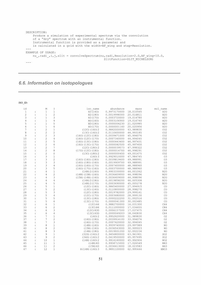
51

DESCRIPTION: Produce a simulation of experimental spectrum via the convolution of a “dry” spectrum with an instrumental function. Instrumental function is provided as a parameter and is calculated in a grid with the width=AF_wing and step=Resolution. --- EXAMPLE OF USAGE: nu_,radi_,i,j,slit = convolveSpectrum(nu,radi,Resolution=2.0,AF_wing=10.0, SlitFunction=SLIT_MICHELSON) ---

__________________________________________________________________________________

6.6. Information on isotopologues

__________________________________________________________________________________

ISO_ID:

id M I iso_name abundance mass mol_name 1 : 1 1 H2(16O) 0.9973170000 18.010565 H2O 2 : 1 2 H2(18O) 0.0019998300 20.014811 H2O 3 : 1 3 H2(17O) 0.0003720000 19.014780 H2O 4 : 1 4 HD(16O) 0.0003106900 19.016740 H2O 5 : 1 5 HD(18O) 0.0000006230 21.020985 H2O 6 : 1 6 HD(17O) 0.0000001160 20.020956 H2O 7 : 2 1 (12C)(16O)2 0.9842000000 43.989830 CO2 8 : 2 2 (13C)(16O)2 0.0110600000 44.993185 CO2 9 : 2 3 (16O)(12C)(18O) 0.0039471000 45.994076 CO2 10 : 2 4 (16O)(12C)(17O) 0.0007340000 44.994045 CO2 11 : 2 5 (16O)(13C)(18O) 0.0000443400 46.997431 CO2 12 : 2 6 (16O)(13C)(17O) 0.0000082500 45.997400 CO2 13 : 2 7 (12C)(18O)2 0.0000039573 47.998322 CO2 14 : 2 8 (17O)(12C)(18O) 0.0000014700 46.998291 CO2 15 : 2 0 (13C)(18O)2 0.0000000450 49.001675 CO2 16 : 3 1 (16O)3 0.9929010000 47.984745 O3 17 : 3 2 (16O)(16O)(18O) 0.0039819400 49.988991 O3 18 : 3 3 (16O)(18O)(16O) 0.0019909700 49.988991 O3 19 : 3 4 (16O)(16O)(17O) 0.0007400000 48.988960 O3 20 : 3 5 (16O)(17O)(16O) 0.0003700000 48.988960 O3 21 : 4 1 (14N)2(16O) 0.9903330000 44.001062 N2O 22 : 4 2 (14N)(15N)(16O) 0.0036409000 44.998096 N2O 23 : 4 3 (15N)(14N)(16O) 0.0036409000 44.998096 N2O 24 : 4 4 (14N)2(18O) 0.0019858200 46.005308 N2O 25 : 4 5 (14N)2(17O) 0.0003690000 45.005278 N2O 26 : 5 1 (12C)(16O) 0.9865400000 27.994915 CO 27 : 5 2 (13C)(16O) 0.0110800000 28.998270 CO 28 : 5 3 (12C)(18O) 0.0019782000 29.999161 CO 29 : 5 4 (12C)(17O) 0.0003680000 28.999130 CO 30 : 5 5 (13C)(18O) 0.0000222200 31.002516 CO 31 : 5 6 (13C)(17O) 0.0000041300 30.002485 CO 32 : 6 1 (12C)H4 0.9882700000 16.031300 CH4 33 : 6 2 (13C)H4 0.0111000000 17.034655 CH4 34 : 6 3 (12C)H3D 0.0006157500 17.037475 CH4 35 : 6 4 (13C)H3D 0.0000049203 18.040830 CH4 36 : 7 1 (16O)2 0.9952620000 31.989830 O2 37 : 7 2 (16O)(18O) 0.0039914100 33.994076 O2 38 : 7 3 (16O)(17O) 0.0007420000 32.994045 O2 39 : 8 1 (14N)(16O) 0.9939740000 29.997989 NO 40 : 8 2 (15N)(16O) 0.0036543000 30.995023 NO 41 : 8 3 (14N)(18O) 0.0019931200 32.002234 NO 42 : 9 1 (32S)(16O)2 0.9456800000 63.961901 SO2 43 : 9 2 (34S)(16O)2 0.0419500000 65.957695 SO2 44 : 10 1 (14N)(16O)2 0.9916160000 45.992904 NO2 45 : 11 1 (14N)H3 0.9958715000 17.026549 NH3 46 : 11 2 (15N)H3 0.0036613000 18.023583 NH3 47 : 12 1 H(14N)(16O)3 0.9891100000 62.995644 HNO3

52

48 : 13 1 (16O)H 0.9974730000 17.002740 OH 49 : 13 2 (18O)H 0.0020001400 19.006986 OH 50 : 13 3 (16O)D 0.0001553700 18.008915 OH 51 : 14 1 H(19F) 0.9998442500 20.006229 HF 52 : 15 1 H(35Cl) 0.7575870000 35.976678 HCl 53 : 15 2 H(37Cl) 0.2422570000 37.973729 HCl 54 : 16 1 H(79Br) 0.5067800000 79.926160 HBr 55 : 16 2 H(81Br) 0.4930600000 81.924115 HBr 56 : 17 1 H(127I) 0.9998442500 127.912297 HI 57 : 18 1 (35Cl)(16O) 0.7559100000 50.963768 ClO 58 : 18 2 (37Cl)(16O) 0.2417200000 52.960819 ClO 59 : 19 1 (16O)(12C)(32S) 0.9373900000 59.966986 OCS 60 : 19 2 (16O)(12C)(34S) 0.0415800000 61.962780 OCS 61 : 19 3 (16O)(13C)(32S) 0.0105300000 60.970341 OCS 62 : 19 4 (16O)(12C)(33S) 0.0105300000 60.966371 OCS 63 : 19 5 (18O)(12C)(32S) 0.0018800000 61.971231 OCS 64 : 20 1 H2(12C)(16O) 0.9862400000 30.010565 H2CO 65 : 20 2 H2(13C)(16O) 0.0110800000 31.013920 H2CO 66 : 20 3 H2(12C)(18O) 0.0019776000 32.014811 H2CO 67 : 21 1 H(16O)(35Cl) 0.7557900000 51.971593 HOCl 68 : 21 2 H(16O)(37Cl) 0.2416800000 53.968644 HOCl 69 : 22 1 (14N)2 0.9926874000 28.006147 N2 70 : 23 1 H(12C)(14N) 0.9851100000 27.010899 HCN 71 : 23 2 H(13C)(14N) 0.0110700000 28.014254 HCN 72 : 23 3 H(12C)(15N) 0.0036217000 28.007933 HCN 73 : 24 1 (12C)H3(35Cl) 0.7489400000 49.992328 CH3Cl 74 : 24 2 (12C)H3(37Cl) 0.2394900000 51.989379 CH3Cl 75 : 25 1 H2(16O)2 0.9949520000 34.005480 H2O2 76 : 26 1 (12C)2H2 0.9776000000 26.015650 C2H2 77 : 26 2 (12C)(13C)H2 0.0219700000 27.019005 C2H2 78 : 27 1 (12C)2H6 0.9769900000 30.046950 C2H6 79 : 28 1 (31P)H3 0.9995328300 33.997238 PH3 80 : 29 1 (12C)(16O)(19F)2 0.9865400000 65.991722 COF2 81 : 31 1 H2(32S) 0.9498800000 33.987721 H2S 82 : 31 2 H2(34S) 0.0421400000 35.983515 H2S 83 : 31 3 H2(33S) 0.0074980000 34.987105 H2S 84 : 32 1 H(12C)(16O)(16O)H 0.9838980000 46.005480 HCOOH 85 : 33 1 H(16O)2 0.9951070000 32.997655 HO2 86 : 34 1 (16O) 0.9976280000 15.994915 O 87 : 36 1 (14N)(16O)+ 0.9939740000 29.997989 NOp 88 : 37 1 H(16O)(79Br) 0.5056000000 95.921076 HOBr 89 : 37 2 H(16O)(81Br) 0.4919000000 97.919027 HOBr 90 : 38 1 (12C)2H4 0.9773000000 28.031300 C2H4 91 : 38 2 (12C)H2(13C)H2 0.0219600000 29.034655 C2H4 92 : 39 1 (12C)H3(16O)H 0.9859300000 32.026215 CH3OH 93 : 40 1 (12C)H3(79Br) 0.5013000000 93.941811 CH3Br 94 : 40 2 (12C)H3(81Br) 0.4876600000 95.939764 CH3Br 95 : 41 1 (12C)H3(12C)(14N) 0.9748200000 41.026549 CH3CN 96 : 42 1 (12C)(19F)4 0.9893000000 87.993616 CF4 97 : 46 1 (12C)(32S) 0.9396240000 43.971036 CS 98 : 46 2 (12C)(34S) 0.0416817000 45.966787 CS 99 : 46 3 (13C)(32S) 0.0105565000 44.974368 CS 100 : 46 4 (12C)(33S) 0.0074166800 44.970399 CS 101 : 1001 1 H -1.0000000000 -1.000000 H 102 : 1002 1 He -1.0000000000 -1.000000 He 103 : 45 1 H2 0.9996880000 2.015650 H2 104 : 1018 1 Ar -1.0000000000 -1.000000 Ar 105 : 26 3 (12C)2HD 0.0003045500 27.021825 C2H2 106 : 27 2 (12C)H3(13C)H3 0.0219526110 31.050305 C2H6 107 : 15 3 D(35Cl) 0.0001180050 36.982954 HCl 108 : 15 4 D(37Cl) 0.0000377350 38.980004 HCl 109 : 44 1 H(12C)3(14N) 0.9646069000 51.010899 HC3N 110 : 14 2 D(19F) 0.0001150000 21.012505 HF 111 : 16 3 D(79Br) 0.0000582935 80.932439 HBr 112 : 16 4 D(81Br) 0.0000567065 82.930392 HBr 113 : 17 2 D(127I) 0.0001150000 128.918575 HI 114 : 47 1 (32S)(16O)3 0.9423964000 79.956820 SO3 115 : 45 2 HD 0.0002299700 3.021825 H2 116 : 43 1 (12C)4H2 0.9559980000 50.015650 C4H2 117 : 12 2 H(15N)(16O)3 0.0036360000 63.992680 HNO3 118 : 22 2 (14N)(15N) 0.0072535000 29.997989 N2 119 : 29 2 (13C)(16O)(19F)2 0.0110834000 66.995083 COF2 120 : 2 11 (18O)(13C)(17O) 0.0000000165 48.001650 CO2 121 : 2 9 (12C)(17O)2 0.0000001368 45.998262 CO2

53

__________________________________________________________________________________

ABUNDANCE:

__________________________________________________________________________________

abundance(M, I) INPUT PARAMETERS: M: HITRAN molecule number I: HITRAN isotopologue number OUTPUT PARAMETERS: Abbundance: natural abundance --- DESCRIPTION: Return natural (Earth) abundance of HITRAN isotolopogue. --- EXAMPLE OF USAGE: ab = abundance(1,1) # H2O ---

__________________________________________________________________________________

MOLECULAR MASS:

__________________________________________________________________________________

molecularMass(M, I) INPUT PARAMETERS: M: HITRAN molecule number I: HITRAN isotopologue number OUTPUT PARAMETERS: MolMass: molecular mass --- DESCRIPTION: Return molecular mass of HITRAN isotolopogue. --- EXAMPLE OF USAGE: mass = molecularMass(1,1) # H2O ---

__________________________________________________________________________________

MOLECULE NAME:

__________________________________________________________________________________

moleculeName(M) INPUT PARAMETERS: M: HITRAN molecule number OUTPUT PARAMETERS: MolName: molecular name --- DESCRIPTION: Return name of HITRAN molecule. --- EXAMPLE OF USAGE: molname = moleculeName(1) # H2O ---

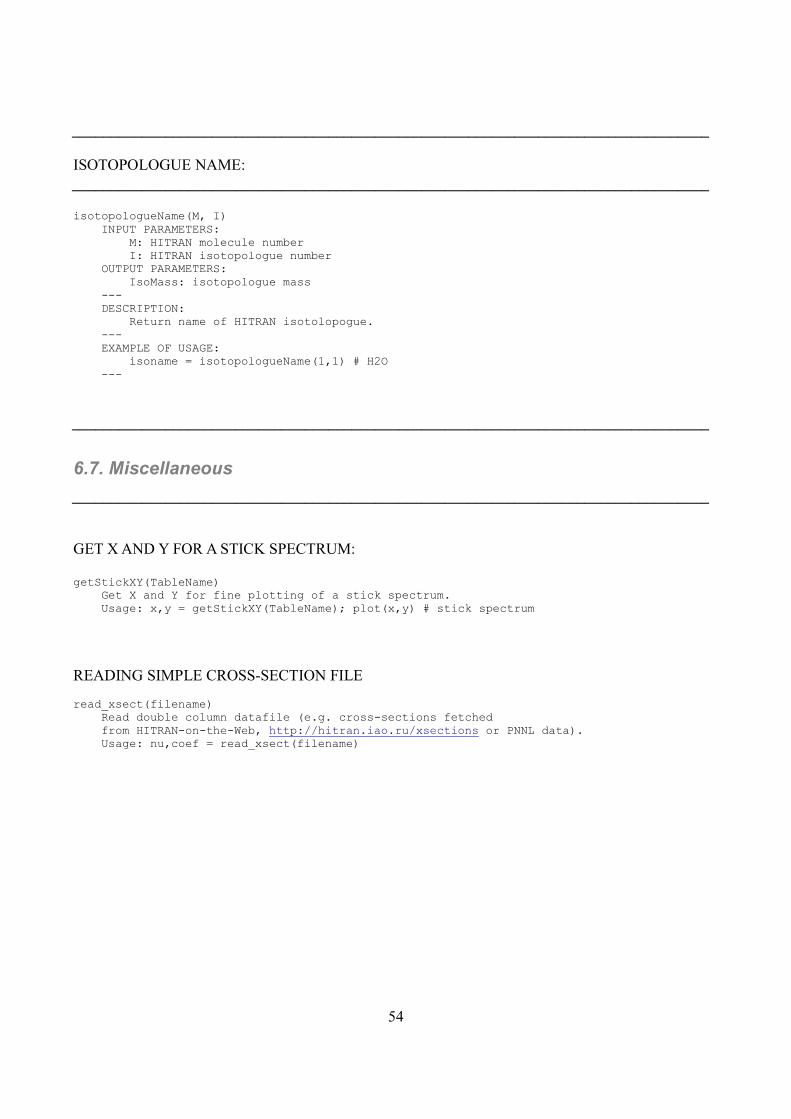
54

__________________________________________________________________________________

ISOTOPOLOGUE NAME:

__________________________________________________________________________________

isotopologueName(M, I) INPUT PARAMETERS: M: HITRAN molecule number I: HITRAN isotopologue number OUTPUT PARAMETERS: IsoMass: isotopologue mass --- DESCRIPTION: Return name of HITRAN isotolopogue. --- EXAMPLE OF USAGE: isoname = isotopologueName(1,1) # H2O ---

__________________________________________________________________________________

6.7. Miscellaneous

__________________________________________________________________________________

GET X AND Y FOR A STICK SPECTRUM:

getStickXY(TableName) Get X and Y for fine plotting of a stick spectrum. Usage: x,y = getStickXY(TableName); plot(x,y) # stick spectrum

READING SIMPLE CROSS-SECTION FILE read_xsect(filename) Read double column datafile (e.g. cross-sections fetched from HITRAN-on-the-Web, http://hitran.iao.ru/xsections or PNNL data). Usage: nu,coef = read_xsect(filename)

55

REFERENCES:

[1] N.H. Ngo, D. Lisak, H. Tran, J.-M. Hartmann.

An isolated line-shape model to go beyond the Voigt profile in

spectroscopic databases and radiative transfer codes.

JQSRT, Volume 129, November 2013, Pages 89–100

http://dx.doi.org/10.1016/j.jqsrt.2013.05.034

[2] H. Tran, N.H. Ngo, J.-M. Hartmann.

Erratum to “Efficient computation of some speed-dependent isolated line profiles”.

JQSRT, Volume 134, February 2014, Pages 104

http://dx.doi.org/10.1016/j.jqsrt.2013.10.015

[3] J. Tennyson, P.F. Bernath, A. Campargue, A.G. Császár, L. Daumont, R.R. Gamache, et al.

Recommended isolated-line profile for representing high-resolution spectroscopic transitions.

Pure and Applied Chemistry, Volume 86 (12), 2014, Pages 1931-1943

http://dx.doi.org/ 10.1515/pac-2014-0208

[4] A. L. Laraia, R. R. Gamache, J. Lamouroux, I. E. Gordon, L. S. Rothman.

Total internal partition sums to support planetary remote sensing.

Icarus, Volume 215, Issue 1, September 2011, Pages 391–400

http://dx.doi.org/10.1016/j.icarus.2011.06.004

[5] L.S. Rothman, I.E. Gordon, Y. Babikov, A. Barbe, D.C. Benner, P.F. Bernath, et al.

The HITRAN2012 molecular spectroscopic database.

JQSRT, Volume 130, 2013, Pages 4-50

http://dx.doi.org/10.1016/j.jqsrt.2013.07.002