fill

Hiring as Exploration∗

Danielle Li Lindsey Raymond Peter BergmanMIT & NBER MIT Columbia & NBER

February 25, 2021

Abstract

This paper views hiring as a contextual bandit problem: to find the best workers over time, firms must balance “exploitation” (selecting from groups with proven track records) with “exploration” (selecting from under-represented groups to learn about quality). Yet modern hiring algorithms, based on “supervised learning” approaches, are designed solely for exploitation. Instead, we build a resume screening algorithm that values exploration by evaluating candidates according to their statistical upside potential. Using data from professional services recruiting within a Fortune 500 firm, we show that this approach improves the quality (as measured by eventual hiring rates) of candidates selected for an interview, while also increasing demographic diversity, relative to the firm’s existing practices. The same is not true for traditional supervised learning based algorithms, which improve hiring rates but select far fewer Black and Hispanic applicants. In an extension, we show that exploration-based algorithms are also able to learn more effectively about simulated changes in applicant hiring potential over time. Together, our results highlight the importance of incorporating exploration in developing decision-making algorithms that are potentially both more efficient and equitable.

JEL Classifications: D80, J20, M15, M51, O33

Keywords: Machine Learning, Hiring, Supervised Learning, Bandit Problems, Algorithmic

Fairness, Diversity.

∗Correspondence to d li@mit.edu, lraymond@mit.edu, and bergman@tc.columbia.edu. We are grateful to David Autor,Pierre Azoulay, Dan Bjorkegren, Emma Brunskill, Max Cytrynbaum, Eleanor Dillon, Alex Frankel, Bob Gibbons, NathanHendren, Max Kasy, Pat Kline, Fiona Murray, Anja Sautmann, Scott Stern, John Van Reenen, Kathryn Shaw, and variousseminar participants for helpful comments and suggestions. The content is solely the responsibility of the authors and does notnecessarily represent the official views of Columbia University, MIT, or the NBER.

Algorithms have been shown to outperform human decision-makers across an expanding range

of settings, from medical diagnosis to image recognition to game play.1 Yet the rise of algorithms is

not without its critics, who caution that automated approaches may codify existing human biases

and allocate fewer resources to those from under-represented groups.2

A key emerging application of machine learning (ML) tools is in hiring, a setting where decisions

matter for both firm productivity and individual access to opportunity, and where algorithms are

increasingly used at the “top of the funnel,” to screen job applicants for interviews.3 Modern hiring

ML typically relies on “supervised learning,” meaning that it forms a model of the relationship

between applicant covariates and outcomes in a given training dataset, and then applies this model

to predict outcomes for subsequent applicants.4 By systematically analyzing historical examples,

these tools can unearth predictive relationships that may be overlooked by human recruiters; indeed,

a growing literature has shown that supervised learning algorithms can more effectively identify

high quality job candidates than human recruiters.5 Yet because this approach implicitly assumes

that past examples extend to future applicants, firms that rely on supervised learning may tend

to select from groups with proven track records, raising concerns about access to opportunity for

non-traditional applicants.6

This paper is the first to develop and evaluate a new class of applicant screening algorithms,

one that explicitly values exploration. Our approach begins with the idea that the hiring process

can be thought of as a contextual bandit problem: in looking for the best applicants over time, a

firm must balance “exploitation” with “exploration” as it seeks to learn the predictive relationship

between applicant covariates (the “context”) and applicant quality (the “reward”). Whereas the

1For example, see Yala et al. (2019); McKinney (2020); Mullainathan and Obermeyer (2019); Schrittwieser et al.(2019); Russakovsky et al. (2015)

2A widely publicized example is Amazon’s use of an automated hiring tool that penalized the use of the term“women’s” (for example, “women’s crew team”) on resumes: https://www.reuters.com/article/us-amazon-com-jobs-automation-insight/amazon-scraps-secret-ai-recruiting-tool-that-showed-bias-against-women-idUSKCN1MK08G. Ober-meyer et al. (2019); Datta et al. (2015); Lambrecht and Tucker (2019) document additional examples in the academicliterature. For additional surveys of algorithmic fairness, see Barocas and Selbst (2016); Corbett-Davies and Goel(2018); Cowgill and Tucker (2019). For a discussion of broader notions of algorithmic fairness, see Kasy and Abebe(2020); Kleinberg et al. (2016).

3A recent survey of technology companies indicated that 60% plan on investing in AI-powered recruiting softwarein 2018, and over 75% of recruiters believe that artificial intelligence will transform hiring practices (Bogen and Rieke,2018).

4ML tools can be used in a variety of ways throughout the hiring process but, by far, algorithms are most commonlyused in the first stages of the application process to decide which applicants merit further human review (Raghavan etal., 2019). In this paper, we will use the term “hiring ML” to refer primarily to algorithms that help make the initialinterview decision, rather than the final offer. For a survey of commercially available hiring ML tools, see Raghavan etal. (2019).

5See, for instance, Hoffman et al. (2018); Cowgill (2018).6For example, Kline and Walters (2020) test for discrimination in hiring practices, which can both be related to

the use of algorithms and influence the data available to them. The relationship between existing hiring practicesand algorithmic biases is theoretically nuanced; for a discussion, see Rambachan et al. (2020); Rambachan and Roth(2019); Cowgill (2018).

1

optimal solution to bandit problems is widely known to incorporate some exploration, supervised

learning based algorithms engage only in exploitation because they are designed to solve static

prediction problems. By contrast, ML tools that incorporate exploration are designed to solve

dynamic prediction problems that involve learning from sequential actions: in the case of hiring,

these algorithms value exploration because learning improves future choices.

Incorporating exploration into screening technologies may also shift the demographic composition

of selected applicants. While exploration in the bandit sense—that is, selecting candidates with

whatever covariates there is more uncertainty over—need not be the same as favoring demographic

diversity, it is also the case that Black, Hispanic, and female applicants are less likely to be employed

in high-income jobs, meaning that they will also appear less often in the historical datasets used to

train hiring algorithms. Because data under-representation tends to increase uncertainty, adopting

bandit algorithms that value exploration (for the sake of learning) may expand representation even

when demographic diversity is not part of their mandate.7

Our paper uses data from a large Fortune 500 firm to study the decision to grant first-round

interviews for high-skill positions in consulting, financial analysis, and data science—sectors which

offer well-paid jobs with opportunities for career mobility and which have also been criticized for

their lack of diversity. In this setting, we provide the first empirical evidence that algorithmic

design impacts access opportunity. Relative to human screening decisions, we show that contextual

bandit algorithms increase the quality of interview decisions (as measured by hiring yield) while

also selecting a more diverse set of applicants. Yet, in the same setting, we also show that this

is not the case for traditional supervised learning approaches, which increase quality but at the

cost of vastly reducing Black and Hispanic representation. Our results therefore demonstrate the

potential of algorithms to improve the hiring process, while cautioning against the idea that they

are generically equity or efficiency enhancing.

Like many firms in its sector, our data provider is overwhelmed with applications and rejects the

vast majority of candidates on the basis of an initial resume screen. Motivated by how ML tools

are typically used in the hiring process, our goal is to understand how algorithms can impact this

consequential interview decision. In our analysis, we focus on hiring yield as our primary measure

of quality. Because recruiting is costly and diverts employees from other productive work, our firm

would like to adopt screening tools that improve its ability to identify applicants who will ultimately

receive and accept an offer; currently, our firm’s hiring rate among those interviewed is only 10%.

7This logic is consistent with a growing number of studies focusing on understanding persistent biases in employerbeliefs, and how to change them. For example, see Miller (2017); Bohren et al. (2019a,b); Lepage (2020a,b). In thesepapers and others, small sample experiences with some minority workers (or some other source of biased priors) maylock firms into persistent inaccurate beliefs about the overall quality of minority applicants. In such cases, firms maybenefit from exploration-based algorithms that nudge them toward obtaining additional signals of minority quality.

2

As such, for most of our analysis, we define an applicant’s quality as her “hiring potential”—that is,

her likelihood of being hired, were she to receive an interview.8

We build three different resume screening algorithms—two based on supervised learning, and

one based on a contextual bandit approach—and evaluate the candidates that each algorithm

selects, relative to the actual interview decisions made by the firm’s human resume screeners. We

observe data on an applicant’s demographics (race, gender, and ethnicity), education (institution

and degree), and work history (prior firms). Our goal is to maximize the quality of applicants who

are selected for an interview; although we will also evaluate their diversity, we do not incorporate

any explicit diversity preferences into our algorithm design.

Our first algorithm uses a static supervised learning approach (hereafter, “static SL”) based on

a logit LASSO model. Our second algorithm (hereafter, “updating SL”) builds on the same baseline

model as the static SL model, but updates the training data it uses throughout the test period with

the hiring outcomes of the applicants it chooses to interview.9 While this updating process allows

the updating SL model to learn about the quality of the applicants it selects, it is myopic in the

sense that it does not incorporate the value of this learning into its selection decisions.

Our third approach implements an Upper Confidence Bound (hereafter, “UCB”) contextual

bandit algorithm: in contrast to the static and updating SL algorithms, which evaluates candidates

based on their point estimates of hiring potential, a UCB contextual bandit selects applicants based

on the upper bound of the confidence interval associated with those point estimates. That is, there

is implicitly an “exploration bonus” that is increasing in the algorithm’s degree of uncertainty

about quality. Exploration bonuses will tend to be higher for groups of candidates who are under-

represented in the algorithm’s training data because the model will have less precise estimates for

these groups. In our implementation, we allow exploration bonuses to be based on a wide set of

applicant covariates: the algorithm can choose to assign higher exploration bonuses on the basis of

race or gender, but it is not required to and the algorithm could, instead, focus on other variables

such as education or work history. Once candidates are selected, we incorporate their realized

hiring outcomes into the training data and update the algorithm for the next period.10 Standard

and contextual bandit UCB algorithms have been shown to be optimal in the sense that they

8Henceforce, this paper will use the terms “quality,” “hiring potential,” and “hiring likelihood” interchangeably,unless otherwise noted.

9In practice, we can only update the model with data from selected applicants who are actually interviewed(otherwise we would not observe their hiring outcome). See Section 3.2.2 for a more detailed discussion of how thisalgorithm is updated.

10Similar to the updating SL approach, we only observe hiring outcomes for applicants who are actually interviewedin practice, we are only able to update the UCB model’s training data with outcomes for the applicants it selects whoare also interviewed in practice. See Section 3.2.3 for more discussion.

3

asymptotically minimize expected regret11 and have begun to be used in economic applications.12

Ours is the first to apply a contextual bandit in the context of hiring.

We have two main sets of results. First, our SL and UCB models differ markedly in the

demographic composition of the applicants they select to be interviewed. Implementing a UCB

model would more than double the share of interviewed applicants who are Black or Hispanic, from

10% to 24%. The static and updating SL models, however, would both dramatically decrease the

combined share of Black and Hispanic applicants to 2% and 5%, respectively. In the case of gender,

all algorithms would increase the share of selected applicants who are women, from 35% under

human recruiting, to 42%, 40%, and 48%, under static SL, updating SL, and UCB, respectively.

This increase in diversity is persistent throughout our sample.

Our second set of results shows that, despite differences in their demographic profiles, all

of our ML models substantial increase hiring yield relative to human recruiters. We note that

assessing quality differences between human and ML models is more difficult than assessing diversity

because we face a sample selection problem, also known in the ML literature as a “selective labels”

problem:13 although we observe demographics for all applicants, we only observe “hiring potential”

for applicants who are interviewed. To address this, we take three complementary approaches, all of

which consistently show that ML models select candidates with greater hiring potential than human

recruiters. We describe these approaches in more detail below.

First, we focus on the sample of interviewed candidates for whom we directly observe hiring

outcomes. Within this sample, we ask whether applicants preferred by our ML models have a higher

likelihood of being hired than applicants preferred by a human recruiter. In order to define a “human

score” that proxies for recruiter preferences, we train a fourth algorithm (a supervised learning

model similar to our static SL) to predict human interview decisions rather than hiring likelihood

(hereafter, “human SL”). We then examine which scores are best able to identify applicants who

are hired. We find that, across all of our ML models, applicants with high scores are much more

likely to be hired than those with low scores. In contrast, there is almost no relationship between

an applicant’s propensity to be selected by a human, and his or her eventual hiring outcome; if

anything, this relationship is negative.

Our second approach estimates hiring potential for the full sample of applicants. A concern with

restricting our analysis to those who are interviewed is that we may overstate the relative accuracy

11Lai and Robbins (1985); Abbasi-Yadkori et al. (2019); Li et al. (2017) prove regret bounds for several differentUCB algorithmns. We follow the approach in Li et al. (2017) that extends the contextual bandit UCB for binaryoutcomes. See Section 2.1 and 3 for a detailed discussion.

12For example, see Currie and MacLeod (2020); Stefano Caria and Teytelboym (2020); Kasy and Sautmann (2019);Bergemann and Valimaki (2006); Athey and Wager (2019); Krishnamurthy and Athey (2020); Zhou et al. (2018);Dimakopoulou et al. (2018a).

13See, for instance, Lakkaraju et al. (2017); Kleinberg et al. (2018a).

4

of our ML models if human recruiters add value by making sure particularly weak candidates are

never interviewed. To address this concern, we use an inverse propensity score weighting approach

to recover an estimate of the mean hiring likelihood among all applicants selected by each of our

ML models using information on the outcomes of interviewed applicants with similar covariates. We

continue to find that ML models select applicants with higher predicted hiring likelihoods, relative

to those selected by humans: average hiring rates among those selected by the UCB, updating SL,

and static SL models are 33%, 35%, and 24%, respectively, compared with the observed 10% among

observed recruiter decisions. These results suggest that, by adopting an ML approach, the firm

could hire the same number of people while conducting fewer interviews.

Finally, we use an IV strategy to explore the robustness of our conclusions to the possibility

of selection on unobservables. So far, our approaches have either ignored sample selection or have

assumed that selection operates on observables only. While there is relatively little scope for selection

on unobservables in our setting (recruiters make interview decisions on the basis of resume review

only), we verify this assumption using variation from random assignment to initial screeners (who

vary in their leniency to grant interviews). In particular, we show that applicants selected by

stringent screeners (and therefore subject to a higher bar) have no better outcomes than those

selected by more lax screeners: this suggests that humans are not positively screening candidates in

their interview decisions.

We use this same IV variation to show that firms can improve their current interview practices

by following ML recommendations on the margin. Specifically, we estimate the hiring outcomes of

instrument compliers, those who would be interviewed only if they are lucky enough to be assigned

to a lenient screener. We show that, among these marginal candidates, those with high UCB scores

have better hiring outcomes and are also more likely to be Black, Hispanic, or female. This indicates

that following UCB recommendations on the margin would increase both the hiring yield and the

demographic diversity of selected interviewees. In contrast, following the same logic, we show that

following SL recommendations on the margin would generate similar increases in hiring yield but

decrease minority representation.

These approaches, each based on different assumptions, all yield the same conclusion: ML models

increase quality relative to human recruiters, but supervised learning models may do so at the cost

of decreased diversity.

An alternative explanation for our findings so far is that firms care about on the job performance

and recruiters may therefore sacrifice hiring likelihood in order to interview candidates who would

perform better in their roles if hired. Our ability to address this concern is unfortunately limited by

data availability: we observe job performance ratings for very few employees in our training period,

making it impossible to train a model to predict on the job performance. We show, however, that

5

our ML models (trained to maximize hiring likelihood) appear more positively correlated with on the

job performance than a model trained to mimic the choices of human recruiters. This suggests that

it is unlikely that our results can be explained by human recruiters successfully trading off hiring

likelihood to maximize other dimensions of quality, insofar as they can be captured by performance

ratings or promotions.

Together, our main findings show that there need not be an equity-efficiency tradeoff when

it comes to expanding diversity in the workplace. Specifically, firms’ current recruiting practices

appear to be far from the Pareto frontier, leaving substantial scope for new ML tools to improve

both hiring rates and demographic representation. Even though our UCB algorithm places no value

on diversity in and of itself, incorporating exploration in our setting would lead our firm to interview

twice as many under-represented minorities while more than doubling its predicted hiring yield. At

the same time, we emphasize that our SL models lead to similar increases in hiring yield, but at

the cost of drastically reducing the number of Black and Hispanic applicants who are interviewed.

This divergence in demographic representation between our SL and UCB results demonstrates the

importance of algorithmic design for shaping access to labor market opportunities.

In addition, we explore two extensions. First, we examine algorithmic learning over time. Our

test data cover a relatively short time period, 2018-2019Q1, so that there is relatively limited scope

for the relationship between applicant covariates and hiring potential to evolve. In practice, however,

this can change substantially over time, both at the aggregate level—due, for instance, to the

increasing share of women and minorities with STEM degrees—or at the organizational level—such

as if firms improve their ability to attract and retain minority talent. To examine how different types

of hiring ML adapt to changes in quality, we conduct simulations in which the hiring potential of

one group of candidates substantially changes during our test period. Our results indicate that the

value of exploration is higher in cases when the quality of traditionally under-represented candidates

is changing.

In a second extension, we explore the impact of blinding the models to demographic variables.

Our baseline ML models all use demographic variables—race and gender—as inputs, meaning that

they engage in “disparate treatment,” a legal gray area.14 To examine the extent to which our

results rely on these variables, we estimate a new model in which we remove demographic variables

as explicit inputs. We show that this model can achieve similar improvements in hiring yield, but

with more modest increases in share of under-represented minorities who are selected. In our data,

we see a greater increase in Asian representation because, despite making up the majority of our

applicant sample, these candidates are more heterogeneous on other dimensions (such as education

14For a detailed discussion of the legal issues involved in algorithmic decision-making, see Kleinberg et al. (2018b).

6

and geography) and therefore receive larger “exploration bonuses” in the absence of information

about race.

The remainder of the paper is organized as follows. Section 1 discusses our firm’s hiring practices

and its data. Section 2 presents the firm’s interview decision as a contextual bandit problem and

outlines how algorithmic interview rules would operate in our setting. Section 3 discuss how we

explicitly construct and validate our algorithms. We present our main results on diversity and quality

in Section 4, while Sections 5 and 6 discuss our learning and demographics-blinding extensions,

respectively.

1 Background

1.0.1 Setting

We focus on recruiting for high-skilled, professional services positions, a sector that has seen

substantial wage and employment growth in the past two decades (BLS, 2019). At the same time,

this sector has attracted criticism for its perceived lack of diversity: female, Black, and Hispanic

applicants are substantially under-represented relative to their overall shares of the workforce (Pew,

2018). This concern is acute enough that companies such as Microsoft, Oracle, Allstate, Dell,

JP Morgan Chase, and Citigroup offer scholarships and internship opportunities targeted toward

increasing recruiting, retention, and promotion of those from low-income and historically under-

represented groups.15 However, despite these efforts, organizations routinely struggle to expand the

demographic diversity of their workforce—and to retain and promote those workers—particularly in

technical positions (Jackson, 2020; Castilla, 2008; Athey et al., 2000).

Our data come from a Fortune 500 company in the United States that hires workers in several

job families spanning business and data analytics. All of these positions require a bachelor’s degree,

with a preference for candidates graduating with a STEM major, a master’s degree, and, often,

experience with programming in Python, R or SQL. Like other firms in its sector, our data provider

faces challenges in identifying and hiring applicants from under-represented groups. As described

in Table 1, most applicants in our data are male (68%), Asian (58%), or White (29%). Black and

Hispanic candidates comprise 13% of all applications, but under 5% of hires. Women, meanwhile,

make up 33% of applicants and 34% of hires.

In our setting, initial interview decisions are a crucial part of the hiring process. Openings for

professional services roles are often inundated with applications: our firm receives approximately

200 applications for each worker it hires. Interview slot are scarce: because they are conducted

15For instance, see here for a list of internship opportunities focused on minority applicants. JP Morgan Chasecreated Launching Leaders and Citigroup offers the HSF/Citigroup Fellows Award.

7

by current employees who are diverted from other types of productive work, firms are extremely

selective when deciding which of these applicants to interview: our firm rejects 95% of applicants

prior to interviewing them. These initial interview decisions, moreover, are made on the basis of

relatively little information: our firm makes interview decisions on the basis of resume review only.

Given the volume of candidates who are rejected at this stage, recruiters may easily make

mistakes by interviewing candidates who turn out to be weak, while passing over candidates who

would have been strong. In addition to mattering for firm productivity, these types of mistakes may

also restrict access to economic opportunity. In particular, when decisions need to be made quickly,

humans may rely on heuristics that may overlook talented individuals who do not fit traditional

models of success (Friedman and Laurison, 2019; Rivera, 2015).

1.0.2 Applicant quality

In our paper, we focus on how firms can improve their interview decisions, as measured by the

eventual hiring rates of interviewed workers—that is, whether they are able to efficiently identify

applicants who “are above the bar.” We focus on this margin because it is empirically important

for our firm, it is representative of commercially available hiring ML, and because we have enough

data on interview outcomes (hiring or not) to train ML models to predict this outcome.

A key challenge that our firm faces is being able to hire qualified workers to meet its labor

demands; yet even after rejecting 95% of candidates in deciding whom to interview, 90% of interviews

do not result in a hire. These interviews are moreover costly because they divert high-skill current

employees from other productive tasks (Kuhn and Yu, 2019). This suggests that there is scope

improve interview practices by either extending interview opportunities to a more appropriate set of

candidates, or reducing the number of interviews needed to achieve current hiring outcomes.

Of course, in deciding whom to interview, firms may also care other objectives: they may look

for applicants who have the potential to become superstars—either as individuals, or in their ability

to manage and work in teams—or they may avoid applicants who are more likely to become toxic

employees (Benson et al., 2019; Deming, 2017; Housman and Minor, 2015; Reagans and Zuckerman,

2001; Schumann et al., 2019). In these cases, a more appropriate measure of applicant quality

would be based on on the job performance. Unfortunately, we do not have enough data to train an

ML model to reliably predict these types of outcomes. In Section 4.2.6, however, we are able to

examine the correlation between ML scores and two measures of on the job performance, which we

observe for a small subset of hired workers. This analysis provides noisy but suggestive evidence

that ML models trained to maximize hiring rates are also positively related to performance ratings

and promotion rates.

8

Finally, we note that all of the quality measures we consider—hiring rates, performance ratings,

and promotion rates—are based on the discretion of managers and therefore potentially subject to

various types of evaluation and mentoring biases (Rivera and Tilcsik, 2019; Quadlin, 2018; Castilla,

2011). With these caveats in mind, we focus on maximizing quality as defined by a worker’s

likelihood of being hired, if interviewed. We formalize this notion in the following section.

2 Conceptual Framework

2.1 Resume Screening: Contextual Bandit Approach

2.1.1 Model Setup

We model the firm’s interview decision as a contextual bandit problem. Decision rules for

standard and contextual bandits have been well studied in the computer science and statistics

literatures (cf. Bubeck and Cesa-Bianchi, 2012). In economics, bandit models have been applied to

study doctor decision-making, ad placement, recommendation systems, and adaptive experimental

design (Thompson, 1933; Berry, 2006; Currie and MacLeod, 2020; Kasy and Sautmann, 2019;

Dimakopoulou et al., 2018b; Bergemann and Valimaki, 2006). Our set up follows Li et al. (2017).

Each period t, the firm see a set of job applicants indexed by i and for each of them must choose

between one of two actions or “arms”: interview or not, Iit ∈ {0, 1}. The firm would only like to

interview candidates it would hire, so a measure of an applicant’s quality is her “hiring potential”:

Hit ∈ {0, 1} where Hit = 1 if an applicant would be hired if she were interviewed. Regardless, the

firm pays a cost, ct, per interview, which can vary exogenously with time to reflect the number of

interview slots or other constraints in a given period. The firm’s “reward” for each applicant is

therefore given by:

Yit =

Hit − ct if Iit = 1

0 if Iit = 0

After each period t, the firm observes the reward associated with its chosen actions.

So far, this set up follows a standard multi-armed bandit (MAB) approach, in which the

relationship between action and reward is invariant. The optimal solution to MAB problems is

characterized by Gittins and Jones (1979) and Lai and Robbins (1985). Our application departs from

this set up because, for each applicant i in period t, the firm also observes a vector of demographic,

education, and work history information, denoted by X ′it. These variables provide “context” that

can inform the expected returns to interviewing a candidate.

In general, the solutions to MABs are complicated by the presence of context. If firms could

perfectly observe how all potential covariates X ′it relate to hiring quality Hit, then it would simply

9

interview the applicants whose quality is predicted to be greater than their cost of interviewing. In

practice, however, the dimension of the context space makes estimating this relationship difficult,

preventing firms from implementing the ideal decision rule.

To make our model more tractable, we follow Li et al. (2010, 2017) and assume that the

relationship between context and rewards follows a generalized linear form. In particular, we write

E[Hit|X ′it] = µ(X ′itθ∗t ), where µ : R→ R is a link function and θ∗t is an unobserved vector describing

the true predictive relationship between covariates X ′it and hiring potential Hit. We allow for the

possibility that this relationship may change over time, to reflect potential changes in either the

demand or supply of skills.

We express a firm’s interview decision for applicant i at time t:

Iit = I(st(X ′it) > ct) (1)

where st(X′it) can be thought of as a score measuring the value the firm places on a candidate with

covariates X ′it at time t. This score can reflect factors such as the firm’s beliefs about a candidate’s

hiring potential and can be a function of both the candidate’s covariates X ′it, as well as the data

available to the firm at time t. As is standard in the literature on bandit problems, we express the

firm’s objective function in terms of choosing an interview policy I to minimize expected cumulative

“regret,” the difference in rewards between the best choice at a given time and the firm’s actual

choice. The firm’s goal is to identify a scoring function st(X′it) that leads it to identify and interview

applicants with Hit = 1 as often as possible.

2.1.2 “Greedy” solutions

Before turning toward more advanced algorithms, we first note that one class of potential

solutions to bandit problems are given by so-called “greedy” or “exploitation only” algorithms.

These types of algorithms ignore the dynamic learning problem at hand and simply choose the arm

with the highest expected reward in the present. In our case, a firm following a greedy solution would

form its best guess of θ∗t given the training data it has available, and then score candidates on their

basis of their expected hiring likelihood, so that Equation (1) becomes: IGreedyit = I(µ(X ′itθt) > ct).

Supervised learning algorithms are designed to implement precisely this type of greedy solution.

That is, a standard supervised learning model forms an expectation of hiring likelihood using the

data it has available at time t and selects applicants based solely on this measure. If this model is

calculated once at t = 0 and invariant thereafter, this decision rule would correspond to our “static

SL” model; if it is re-estimated in each period to incorporate new data, then this is equivalent to

our “updating SL” model.

10

2.1.3 Exploration-based solutions

It is widely known, however, that greedy algorithms are inefficient solutions to contextual bandit

problems because they do not factor the ex post value of learning into their ex ante selection

decisions (Dimakopoulou et al., 2018b).16

While there is in general no generic optimal strategy for contextual bandits, an emerging literature

in computer science focuses on developing a range of computationally tractable algorithms that

work well in practice.17 For example, recently proposed contextual bandit algorithms include UCB

Auer (2002), Thompson Sampling (Agrawal and Goyal (2013)), and LinUCB (Li et al. (2010)).18

All of these algorithms share the feature that they will sometimes select candidates who do not have

the highest expected quality, but whose interview outcomes could improve the estimates of hiring

potential in the future.

We follow Li et al. (2017) and implement a generalized linear model version of the UCB algorithm,

which assumes that E[Hit|X ′it] follows the functional form given by µ(X ′itθ∗t ), as discussed above.19

Given this assumption, Li et al. (2017) shows that the optimal solution assigns a candidate to the

arm (interview or not) with the highest combined expected reward and “exploration bonus.”20

Exploration bonuses are assigned based on the principle of “optimism in the face of uncertainty”:

the more uncertain the algorithm is about the quality of a candidate based on her covariates,

the higher the bonus she receives. This approach encourages the algorithm to focus on reducing

uncertainty, and algorithms based on this UCB approach have been shown to be asymptotically

efficient in terms of reducing expected regret (Lai and Robbins, 1985; Li et al., 2017; Abbasi-Yadkori

et al., 2019). We discuss the specifics of our implementation and discuss theoretical predictions in

the next section.

16Bastani et al. (2019) show that exploration-free greedy algorithms (such as supervised learning) are generallysub-optimal.

17In particular, the best choice of algorithm for a given situation will depend on the number of possible actions andcontexts, as well as on assumptions regarding the parametric form relating context to reward.

18In addition, see Agrawal and Goyal (2013), and Bastani and Bayati (2019). Furthermore, the existing literaturehas provided regret bounds—e.g., the general bounds of Russo and Roy (2015), as well as the bounds of Rigollet andZeevi (2010) and Slivkins (2014) in the case of non-parametric function of arm rewards—and has demonstrated severalsuccessful applications areas of application—e.g., news article recommendations (Li et al. (2010)) or mobile health(Lei et al. (2017)). For more general scenarios with partially observed feedback, see Rejwan and Mansour (2019) andBechavod et al. (2020). For more on fairness and bandits, see Joseph et al. (2016) and Joseph et al. (2017).

19Li et al. (2017) generalizes the classic general LinUCB algorithm for nonlinear relationship between context andreward. Theorem 2 of that paper gives the regret bound and Equation 6 shows the algorithm implementation wefollow.

20In particular Li et al. (2017) show that the GLM-UCB algorithm has a regret bound of order O(d√T ), where d is

the number of covariates and T is the number of rounds.

11

3 Algorithm Construction

3.1 Data

We have data on 88,666 job applications from January 2016 to April 2019, as described in Table

1. We divide this sample up into two periods, the first consisting of the 48,719 applicants that

arrive before 2018 (2,617 of whom receive an interview), and the second consisting of the 39,947

applications that arrive in 2018-2019 (2,275 of whom are interviewed). We begin by training a

supervised learning model on the 2016-2017 period and testing its out-of-sample validity on the

2018-2019 data. This serves as our “static” supervised learning baseline. In addition, we build an

“updating” supervised learning model, as well as a contextual bandit UCB model. Both of these

models begin with the 2016-2017 trained baseline model but continue to train and learn on the

2018-2019 sample. We build our initial “training” dataset using the earliest years of our sample

(rather than taking a random sample) in order to more closely approximate actual applications of

hiring ML, in which firms would likely use historical data to train a model that is then applied

prospectively.

3.1.1 Input Features

We have information on applicants’ educational background, work experience, referral status,

basic demographics, as well as the type of position to which they applied. Appendix Table A.1

provides a list of these raw variables, as well as some summary statistics. We have self-reported

race (White, Asian, Hispanic, Black, not disclosed and other), gender, veteran status, community

college experience, associate, bachelor, PhD, JD or other advanced degree, number of unique

degrees, quantitative background (defined having a degree in a science/social science field), business

background, internship experience, service sector experience, work history at a Fortune 500 company,

and education at elite (Top 50 ranked) US or non-US educational institution. We record the

geographic location of education experience at an aggregated level (India, China, Europe). We also

track the job family each candidate applied to, the number of applications submitted, and the time

between first and most recent application.

To transform this raw information into usable inputs for a machine learning model, we create

a series of categorical and numerical variables that serve as “features” for each applicant. We

standardize all non-indicator features to bring them into the same value range. Because we are

interested in decision-making at the interview stage, we only use information available as of the

application date as predictive features. Our final model includes 106 input features.

12

3.1.2 Interview Outcomes

Each applicant has an indicator for whether they received an interview. Depending on the job

family, anywhere from 3-10% of applicants receive an interview. Among candidates chosen to be

interviewed, we observe interview ratings, whether the candidate received an offer, and whether

the candidate accepted and was ultimately hired. Roughly 20% of candidates who are interviewed

receive an offer and, of them, approximately 50% accept and are hired. We will focus on the final

hiring outcome as our measure of an applicant’s quality, keeping in mind that this is a potential

outcome that is only observed for applicants who are actually interviewed.

Finally, for 180 workers who are hired and have been employed for at least 6 months, we observe

a measure of performance ratings on the job. Because this number is too small to train a model on,

we will use these data to examine the relationship between maximizing hiring likelihood and on the

job performance.

3.2 Models

Here we describe how we construct three distinct interview policies based on static and updating

supervised learning, and contextual bandit UCB. For simplicity, we will sometimes write IML to

refer to the interview policy of any of these ML models.

3.2.1 Static Supervised Learning (“SSL” or “static SL”)

We first use a standard supervised learning approach to predict an applicant’s likelihood of

being hired, conditional on being interviewed. At any given time t (which indexes an application

round that we observe in the testing period) applicants i are selected according to the following

interview policy, based on Equation (1) of our conceptual framework:

ISSLit = I(sSSL0 (X ′it) > ct), where sSSL0 (X ′it) = E[Hit|X ′it;D0] (2)

Here, we emphasize that the firm’s estimate of hiring potential at time t depends on the training

data that it has available at the time. In the static SL model, we write this data as D0 to emphasize

that it is determined at time t = 0 and is not subsequently updated. Using this data, we form an

estimate of sSSL(X ′it) using a L1-regularized logistic regression (LASSO), fitted using three-fold

cross validation.21

21Following best practices as described in Kaebling (2019), we randomly subsample our training data to create abalanced sample, half of whom are hired and half of whom are not hired. Our results are also robust to using anensemble logit lasso and random forest approach, which delivers slightly higher predictive validity (0.67 vs. 0.64 AUC).In our paper, we choose to stick to the simple logit model for transparency and to ensure consistency with our UCBmodel, which is based on Li et al. (2017)’s implementation that uses a logit model to predict expected quality.

13

We evaluate out-of-sample performance on randomly-selected balanced samples from our 2018-

2019 “testing” period after training our models on the 2016-2017 sample. Appendix Figure A.1

plots the receiver operating characteristic (ROC) curve and its associated AUC, or area under the

curve. These are standard measure of predictive performances that quantify the trade-off between a

model’s true positive rate and its false positive rate as the probability threshold for declaring an

observation as hired varies. The AUC is equal to the probability our model with rank a randomly

chosen hired interviewee greater than a randomly chosen applicant who was not hired.22 Our model

has an AUC of .64, meaning that it will rank an interviewed applicant who is hired higher than an

interviewed but not hired applicant 64 percent of the time. We also plot the confusion matrix in

Appendix Figure A.2, which further breaks down the model’s classification performance.

Finally, we note that training on candidates selected by human recruiters lead to biased predictions

because of selection on unobservables. While we believe that there is relatively little scope for

selection on unobservables in our setting (because we observe essentially the same information as

recruiters, who conduct resume reviews without interacting with candidates), we acknowledge the

potential for such bias. Another approach that is commonly used by commercial vendors of hiring

algorithms is to set Hit = 0 for all applicants who are not interviewed. We choose not to follow this

approach as it runs counter to our view that Hit should be thought of as a potential outcome and

because Rambachan and Roth (2019) show that such an approach often leads to algorithms that

are more biased against racial minorities. There are also a growing set of advanced ML tools that

seek to correct for training-sample selection.23 While promising, testing these approaches is outside

of the scope of this paper, and we are not aware of any commercially-available hiring ML that does

attempt to correct for sample selection.24

Taken together, we emphasize that the ML models we build should not be thought of as an

optimal ML model in either its design or its performance but as an example of what could be

feasibly achieved by most firms able to organize their administrative records into a modest training

dataset, with a standard set of resume-level input features, using a standard ML toolkit.25

3.2.2 Updating Supervised Learning (“USL” or “updating SL”)

Our second model presents a variant of the static SL model in which we begin with the same

baseline model as the static SL, but actively update the model as it makes decisions during the

22Formally, the AUC is Pr(s(X ′it) > s(X ′jt)|Hit = 1, Hjt = 0).23See, for example, Dimakopoulou et al. (2018a), Dimakopoulou et al. (2018b) which discuss doubly robust estimators

to remove sample selection and Si et al. (2020).24Raghavan et al. (2019) surveys the methods of commercially available hiring tools and finds that the vast majority

of products marketed as “artificial intelligence” do not use any ML tools at all, and that the few that do simplypredict performance using a static training dataset.

25We would ideally like to compare our AUC to those of commercial providers, but Raghavan et al. (2019) reportsthat no firms currently provide information on the validation of their models.

14

2018-2019 period. That is, we start with a model that is trained on the 2016-2017 data, allow it to

make selection decisions in the 2018-2019 period, but then also update its training data to reflect

the outcomes of these newly selected applicants.26 Once the training data is updated, we retrain

the model and use its updated predictions to make selection decisions in the next round. At any

given point t, the updating SL’s interview decision for applicant i is given by:

IUSLit = I(sUSL

t (X ′it) > ct), where sUSLt (X ′it) = E[Hit|X ′it;DUSL

t ]. (3)

Here, DUSLt is the training data available to the algorithm at time t.

It is important to emphasize that we can only update the model’s training data with observed

outcomes for the set of applicants selected in the previous period: that is, DUSLt+1 = DUSL

t ∪(IUSLt ∩It).

Because we cannot observe hiring outcomes for applicants who are not interviewed in practice, we

can only update our data with outcomes for applicants selected by both the model and by actual

human recruiters. This may impact the degree to which the updating SL model can learn about the

quality of the applicants it selects, relative to a world in which hiring potential is fully observed for

all applicants and we discuss this in more detail shortly, in Section 3.2.4.

3.2.3 Upper Confidence Bound (“UCB”)

As discussed in Section 2.1, we implement a UCB-GLM algorithm as described in Li et al. (2017).

We calculate predicted quality E[Hit|X ′it;DUCBt ] using a regularized logistic regression (Cortes,

2019). At time t = 0 of the testing sample, our UCB and SL models share the same predicted

quality estimate, which is based on the baseline model trained on the 2016-2017 sample. Our UCB

model, however, makes interview decisions for applicant i in period t based on a different scoring

function:

IUCBit = I(sUCB

t (X ′it) > ct), where sUCBt (X ′it) = E[Hit|X ′it;DUCB

t ] + αB(X ′it;DUCBt ). (4)

In Equation (4), the scoring function sUCBt (X ′it) is a combination of the algorithm’s expectations

of an applicant’s quality based on its training data and an exploration bonus that varies with an

applicant’s covariates X ′it. Following the model described in Section 2.1, we assume that E[Hit|X ′it]can be expressed as a generalized linear function µ(X ′itθ

∗t ). In our specific implementation, we

assume that µ is a logistic function and, in each round t, estimate θ∗t using a maximum likelihood

26Specifically, we divide the 2018-2019 data up into “rounds” of 100 applicants. After each round, we take theapplicants the model has selected and update its training data with the outcomes of these applicants, for the subset ofapplicants for whom we observe actual hiring outcomes.

15

estimator so that E[Hit|X ′it;DUCBt ] = µ(X ′itθt

UCB). Next, we calculate the exploration bonus as

B(X ′it;DUCBt ) =

√(Xit − Xt)′V

−1t (Xit − Xt), where Vt =

∑j∈DUCB

t

(Xjt − Xt)(Xjt − Xt)′. (5)

Intuitively, Equation (4) breaks down the value of an action into an exploitation component and

an exploration component. In any given period, a strategy that prioritizes exploitation would choose

to interview a candidate on the basis of her expected hiring potential: this is encapsulated in the

first term, E[Hit|X ′it;DUCBt ]. In contrast, a strategy that prioritizes exploration would choose to

interview a candidate on the basis of the distinctiveness of her covariates; this is encapsulated in the

second term, B(X ′it;DUCBt ), which shows that applicants receive higher bonuses if their covariates

deviate from the mean in the population (Xit − Xt), especially for variables X ′it that generally have

little variance, as seen in the training data (weighted by the precision matrix V −1t ). To balance

exploitation and exploration, Equation (4) combines these two terms so that candidates are judged

not only their mean expected quality, but rather on the mean plus standard error of their estimated

quality—hence the term upper confidence bound. Li et al. (2017) shows that following such a

strategy asymptotically minimizes regret in our setting.

As with the updating SL model, we update the UCB model’s training data with the outcomes

of applicants it has selected—DUCBt+1 = DUCB

t ∪ (IUCBt ∩ It). Based on these new training data, the

UCB algorithm updates both its beliefs about hiring potential and the bonuses it assigns. As was

the case with the updating SL model, we can only add applicants who are selected by the model

and also interviewed in practice. We now turn to the implications of this sample selection.

3.2.4 Feasible versus Live Model Implementation

In a live implementation, each algorithm would select which applicants to interview, and the

interview outcomes for these applicants would be recorded. Our retrospective analysis is limited by

the fact that we only observe interview outcomes for applicants who were actually interviewed (as

chosen by the firm’s human screeners) and, as such, we are only able to update our USL and UCB

models with outcomes for candidates in the intersection of human and algorithmic decision making.

Here, we discuss how the actual interpretation of our models—which we term “feasible” USL or

UCB—may differ from a live implementation.

For concreteness, suppose that in period 1 of our analysis, the UCB model wants to select 50

Black applicants with humanities degrees in order to explore the applicant space. But, in practice,

only 5 such applicants are actually interviewed. In our feasible implementation, we would only be

able to update the UCB’s training data with the outcomes of these 5 applicants, whereas in a live

implementation, we would be able to update with outcomes for all 50 UCB-selected candidates.

16

We first consider the case in which there is no selection on unobservables on the part of the

human recruiters. In this case, the feasible UCB model’s estimates of the expected quality of

Black humanities majors next period would be the same as the live UCB’s estimates, because, in

expectation, the quality of the 5 applicants it was able to learn about is the same as the quality

of the 50 applicants it wanted to learn about. That said, the feasible UCB model would have

considerably more uncertainty about the quality of this population relative to a live UCB, because

its updated estimates are based on 5 applicants rather than 50. This uncertainty would show up in

the next period via the exploration bonus term of Equation (4): even though it has the same beliefs

about quality, the feasible UCB would likely select more Black humanities majors in the next period

relative to a live UCB because it was not able to learn as much, due to limited updating. In this

way, selection on observables should be thought of as slowing down the process of learning for our

UCB (and USL) models. In the limit, the feasible and live UCB (and USL) models should converge

to the same beliefs regarding the quality of the applicants they observe. This would translate into

the same actions because, with a large enough sample, there would be little uncertainty driving

exploration bonuses.27

Next, we consider the case in which human recruiters screen on variables that are unobserved to

us. A particularly concerning version of this type of selection occurs if human recruiters positively

screen on unobservables, so that E[Hit|X ′it, I = 1] > E[Hit|X ′it]. In this case, the 5 Black humanities

majors that are actually selected by human interviewers will tend to be higher quality than the 50

Black humanities majors that the UCB model wanted to select. This means that our feasible UCB

model will be too optimistic about the quality of this population, relative to a live UCB model

that would learn about the quality of all 50 applicants. In the next period, the feasible UCB model

will select more Black humanities majors than a live implementation, both because uncertainty for

these applicants remains higher and because selection on unobservables introduces upwardly biased

beliefs. This latter bias can lead the feasible and live UCB models to select different applicants in

the long run. Specifically, our approach may select too many applicants from groups whose weaker

members are screened out of the model’s training data by human recruiters.

In Section 4.2.4, we discuss the possibility of selection on unobservables in more detail, and

provide IV-based evidence that human recruiters do not appear to be selecting on unobservables.

In addition, Section 5 shows simulation results in which we are able to observe outcomes for all

ML-selected candidates. This allows us to explore the learning behavior of our USL and UCB

27Formally, the distinction between the feasible and live versions of our ML models is related to regression in whichoutcomes are missing at random conditional on unobservables. Under the assumption of no selection on unobservables,common support, and well-specification of the regression function (in our case, the logit), the feasible and live versionsof our models should both be consistent estimators of the underlying parameter θ∗ linking covariates with hiringoutcomes: E[Hit|X ′it] = µ(X ′itθ

∗t ) (Wang et al., 2010; Robins et al., 1995). In finite sample, of course, the point

estimates of the feasible and live models may differ.

17

models in various settings that more closely approximate a live implementation. Finally, in Section

4.2.3 we provide evidence that there is common support amongst the applicants chosen by our ML

models and who is chosen by human recruiters.

3.3 Comparison of SL and UCB models

The use of static SL, updating SL, and UCB models can potentially lead to a variety of differences

in the composition and quality of selected applicants in both the short and long term. Before

describing our empirical results, we focus on the theoretical differences between these models in

terms of both quality and demographic diversity.

3.3.1 Quality of Selected Applicants

As discussed in Section 2, theory predicts that while models that focus on exploration may end

up selecting applicants with lower expected hiring potential in the short run (relative to SL models),

they should eventually minimize regret via more efficient learning (Li et al., 2017; Dimakopoulou et

al., 2018b).

In the long run, the quality of selection decisions made by the UCB and SL algorithms may

or may not differ. One possibility is that, despite selecting different candidates in earlier periods,

both algorithms eventually observe enough examples to arrive at similar estimates of quality for all

applicants: E[Hit|X ′it;DUCBt ] = E[Hit|X ′it;DUSL

t ] for sufficiently large t. If this were the case, then

both UCB and SL models will make the same interview decisions in the long run.

It is also possible, however, for the two types of algorithms to make persistently different

interview decisions, even after many periods. To see this, suppose that we observe only one covariate,

X ∈ {0, 1}, designating group membership, and E[H|X = 0] = 0.2 while E[H|X = 1] = 0.4.

Suppose that the cost of interviewing is 0.3 so that the firm would like to interview all X = 1

candidates and no X = 0 candidates. Suppose, however, that the firm’s initial training data D0

consists of three candidates total: two X = 0 applicants with H = 1 and H = 0 and only one X = 1

applicant with H = 0. A static SL model trained on these data would predict E[H|X = 0;D0] = 0.5

while E[H|X = 1;D0] = 0 and therefore interview all X = 0 candidates and no X = 1 candidates

in the next period. Moreover, because its training data is never updated, it will continue to do

this no matter what outcomes are realized in the future. Meanwhile, an updating SL model would

continue selecting X = 0 candidates until it encounters a sufficient number with H = 0 such that

E[H|X = 0, DUSLt ] < 0.3. However, because E[H|X = 1;D0] = 0, it will never select any X = 1

candidates and therefore never have the opportunity to learn about their quality.

By contrast, a UCB based approach would evaluate candidates on the basis of both their expected

quality and their statistical distinctiveness. Thus, even though X = 1 candidates begin with an

18

expected quality of 0, they would receive an exploration bonus of√

2/3, meaning that the UCB

model would choose to interview X = 1 candidates next period, increasing its chances of learning

about their true expected quality, 0.6.

In our data, differences in the quality of applicants selected by our models will be based on

a combination of their short and long run behaviors. Further, the extent to which the long term

benefits of learning outweigh the short term costs of exploration will also depend on the specifics of

our empirical setting. In particular, when the true relation between applicant covariates and hiring

potential is fixed, and when there is relatively rich initial training data, SL models may perform as

well as if not better than UCB models because the value of exploration will be limited. If, however,

the training data were sparse or if the predictive relation between context and rewards evolves over

time, then the value of exploration is likely to be greater.

3.3.2 Diversity of Selected Applicants

All of our models are designed to maximize applicant quality, as defined by hiring rates, and have

no additional preferences related to diversity. Any differences in the demographics of the candidates

they choose to select will be based on the predictive relation between demographic variables and

hiring outcomes, and will depend on the specifics of our empirical set up.

As can be seen in Equation (5), contextual bandit UCB algorithms are designed to favor

candidates with distinctive covariates, because this helps the algorithm learn more about the

relationship between context (e.g. applicant covariates) and rewards (e.g. hiring outcomes).

This suggests that a UCB model would—at least in the short run—select more applicants from

demographic groups that are under-represented in its training data, relative to SL models. This

tendency to favor demographic minorities, however, will depend on the extent to which demographic

minorities are also minorities along other dimensions such as educational background and work

history. Asian applicants, for example, make up the majority of our applicant sample and so would

receive low exploration bonuses on the basis of race alone; however, they are also more likely to

have non-traditional work histories or have gone to smaller international colleges, factors that make

them appear more distinctive to the UCB model. In our UCB implementation, we place greater

exploration weight on applicants who are distinctive on dimensions in which candidates in the

training data have been relatively homogenous.

As discussed above, long run differences in selection patterns between SL and UCB models are

driven by differences in beliefs. That is, even if the UCB model initially selects more demographic

minorities because it assigns them larger exploration bonuses, this would impact long run differences

in diversity between UCB and SL models only insofar as it generates differences training data that

lead to differences in beliefs: E[Hit|X ′it;DUCBt ] vs. E[Hit|X ′it;DUSL

t ].

19

While we (eventually) expect UCB models to outperform SL models in terms of maximizing

applicant quality, it is unclear this would result in more diversity. For example, it is possible for

exploration to work against minority applicants. To see this, suppose that a UCB model initially

selects more Hispanic applicants in order to explore. If the additional Hispanic applicants it selects

have worse hiring outcomes than those selected by the SL model, the UCB model would enter the

next period with worse beliefs about the hiring potential of Hispanic applicants, relative to the SL.

In sum, the impact of adopting SL vs. UCB models on diversity will depend on the nature of

the training data that the models start with, and with how applicant covariates are actually related

to hiring outcomes. In the next section, we explore these patterns in our main test data; in Section

5, we consider how these results might differ when we conduct simulations that change applicant

quality.

4 Main Results

We now turn to discussing our main results. For notational simplicity, we suppress the subscripts

for applicant i at time t for the remainder of the paper except as needed for clarity.

4.1 Impacts on Diversity of Interviewed Applicants

4.1.1 Overall Representation

We begin by assessing the impact of each policy on the diversity of candidates selected for an

interview in our test sample. This is done by comparing E[X|I = 1], E[X|ISSL = 1], E[X|IUSL = 1],

and E[X|IUCB = 1], for various demographic measures X, where we choose to interview the same

number of people as the actual recruiter. This analysis is straightforward in the sense that we

observe demographic covariates such as race and gender for all applicants so that we can easily

examine differences in the composition of applicants selected by each of the interview policies

described above.

We begin by assessing the racial composition of selected applicants. At baseline, 54% of applicants

in our test sample are Asian, 25% are White, 8% are Black, and 4% are Hispanic. Panel A of Figure

1 shows that, from this pool, human recruiters select a similar proportion of Asian and Hispanic

applicants (57% and 4%, respectively), but relatively more White and fewer Black applicants (34%

and 5%, respectively).

Panels B-D describe our main result with respect to racial diversity: relative to humans, both

SL models sharply reduce the share of Black and Hispanic candidates who are selected, while the

UCB model sharply increases it. Panel B illustrates this in case of static SL, the approach most

commonly used by commercial vendors of hiring ML: the combined share of selected applicants who

20

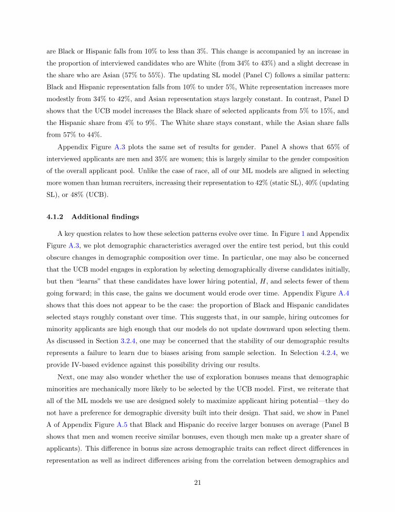
are Black or Hispanic falls from 10% to less than 3%. This change is accompanied by an increase in

the proportion of interviewed candidates who are White (from 34% to 43%) and a slight decrease in

the share who are Asian (57% to 55%). The updating SL model (Panel C) follows a similar pattern:

Black and Hispanic representation falls from 10% to under 5%, White representation increases more

modestly from 34% to 42%, and Asian representation stays largely constant. In contrast, Panel D

shows that the UCB model increases the Black share of selected applicants from 5% to 15%, and

the Hispanic share from 4% to 9%. The White share stays constant, while the Asian share falls

from 57% to 44%.

Appendix Figure A.3 plots the same set of results for gender. Panel A shows that 65% of

interviewed applicants are men and 35% are women; this is largely similar to the gender composition

of the overall applicant pool. Unlike the case of race, all of our ML models are aligned in selecting

more women than human recruiters, increasing their representation to 42% (static SL), 40% (updating

SL), or 48% (UCB).

4.1.2 Additional findings

A key question relates to how these selection patterns evolve over time. In Figure 1 and Appendix

Figure A.3, we plot demographic characteristics averaged over the entire test period, but this could

obscure changes in demographic composition over time. In particular, one may also be concerned

that the UCB model engages in exploration by selecting demographically diverse candidates initially,

but then “learns” that these candidates have lower hiring potential, H, and selects fewer of them

going forward; in this case, the gains we document would erode over time. Appendix Figure A.4

shows that this does not appear to be the case: the proportion of Black and Hispanic candidates

selected stays roughly constant over time. This suggests that, in our sample, hiring outcomes for

minority applicants are high enough that our models do not update downward upon selecting them.

As discussed in Section 3.2.4, one may be concerned that the stability of our demographic results

represents a failure to learn due to biases arising from sample selection. In Selection 4.2.4, we

provide IV-based evidence against this possibility driving our results.

Next, one may also wonder whether the use of exploration bonuses means that demographic

minorities are mechanically more likely to be selected by the UCB model. First, we reiterate that

all of the ML models we use are designed solely to maximize applicant hiring potential—they do

not have a preference for demographic diversity built into their design. That said, we show in Panel

A of Appendix Figure A.5 that Black and Hispanic do receive larger bonuses on average (Panel B

shows that men and women receive similar bonuses, even though men make up a greater share of

applicants). This difference in bonus size across demographic traits can reflect direct differences in

representation as well as indirect differences arising from the correlation between demographics and

21

other variables that also factor into bonus calculations. Appendix Figure A.6 plots the proportion of

the total variation in exploration bonuses that can be attributed to different categories of applicant

covariates. We find that the greatest driver of variation in exploration bonuses is an applicant’s

work history variables, not his or her demographics.

Finally, it is important to note that the results in Figure 1 and Appendix Figure A.3 are based

on the pattern of applicants that the algorithm happens to see in our data. If a different set of

applicants had applied to our sample firm—or if a different set had been interviewed—then it is

possible that our results would change. In Section 5, we will explore how the SL and UCB algorithms

behave under simulations in which the quality of applicants of different groups is changing over

time.

4.2 Impacts on Quality of Interviewed Applicants

4.2.1 Overview

Next, we ask if and to what extent the gains in diversity made by the UCB model come at the

cost of quality, as measured by an applicant’s likelihood of actually being hired. To assess this,

we would ideally like to compare the average hiring likelihoods of applicants selected by each of

the ML models to the actual hiring likelihoods of those selected by human recruiters: E[X|I = 1],

E[X|ISSL = 1], E[X|IUSL = 1], and E[X|IUCB = 1].

Unlike demographics, however, an applicant’s hiring potential H is an outcome that is only

observed when applicants are actually interviewed. We therefore cannot directly observe hiring

potential for applicants selected by either algorithm, but not by the human reviewer. To address

this, we take three complementary approaches, described in turn below. Across all three approaches,

we find evidence that both SL and UCB models—despite their differing demographics—would select

applicants with greater hiring potential than those select using current human recruiting practices.

4.2.2 Interviewed sample

Our first approach compares the quality of applicants selected by our algorithms among the

sample of applicants who are interviewed. However, because all applicants in this sample are—by

definition—selected by human recruiters, we cannot directly compare the accuracy of algorithmic to

human choices within this sample, because there is no variation in the latter.

To get around this, we train an additional model to predict an applicant’s likelihood of being

selected by for an interview, by a human recruiter. That is, we generate a model of E[I|X] where

I ∈ {0, 1} are realized human interview outcomes, using same ensemble approach described in

22

Section 3.2.1.28. This model allows us to order interviewed applicants in terms of their “human

score,” sH , in addition to their algorithmic scores, sSSL, sUSL, and sUCB.29 Appendix Figure

A.7 plots the ROC associated with this model. Our model ranks a randomly chosen interviewed

applicant ahead of a randomly chosen applicant who is not interviewed 76% of the time.30

Figure 2 plots a binned scatterplot depicting the relationship between algorithm scores and hiring

outcomes among the set of interviewed applicants; each dot represents the average hiring outcome

for applicants in a given scoring ventile. Appendix Table A.2 shows these results as regressions

to test whether the relationships are statistically significant. We find that, among those who are

interviewed, applicants’ human scores are uninformative about their hiring likelihood; if anything

this relationship is slightly negative. In contrast, all ML scores have a statistically significant,

positive relation between algorithmic priority selection scores and an applicant’s (out of sample)

likelihood of being hired.

Table 2 examines how these differences in scores translate into differences in interview policies.

To do so, we consider “interview” strategies that select the top 25, 50, or 75% of applicants as

ranked by each model; we then examine how often these policies agree on whom to select, and

which policy performs better when they disagree. Panel A compares the updating SL model to the

human interview model and shows that the human model performs substantially worse in terms

of predicting hiring likelihood when the models disagree: only 5-8% of candidates favored by the

human model are eventually hired, compared with 17-20% of candidates favored by the updating

SL model. Panel B finds similar results when comparing the human model to the UCB model.

Finally, Panel C shows that, despite their demographic differences, the updating SL and UCB

models agree on a greater share of candidates relative to the human model, and there do not appear

to be significant differences in overall hiring likelihoods when they disagree: if anything, the UCB

model performs slightly better.

For consistency, Appendix Figure A.9 revisits our analysis of diversity using the same type of

selection rule described in this section: specifically, picking the top 50% of candidates among the set

of interviewed. Again, we find that UCB selects a substantially more diverse set of candidates than

SL models.

28The only methodological difference between this model and our baseline static SL model is that, because we aretrying to predict interview outcomes as opposed to hiring outcomes conditional on interview, our training sampleconsists of all applicants in the training period, rather than only those who are interviewed.

29Later in this section, we will discuss results that do not require us to model human interview practices.30Although a “good” AUC number is heavily context specific, a general rule of thumb is that models with an AUC

in the range of 0.75− 0.85 have acceptable discriminative properties, depending on the specific context and shape ofthe curve (Fischer et al., 2013).

23

4.2.3 Full sample

A concern with our analysis on the I = 1 sample is that human recruiters may add value by

screening out particularly poor candidates so that they are never observed in the interview sample

to begin with. In this case, then we may see little relation between human preferences and hiring

potential among those who are interviewed, even though human preferences are highly predictive of

quality in the full sample.

To explore this possibility, we attempt to estimate the average quality of all ML-selected

applicants, E[H|IML = 1]. Doing so requires us to assume that there is no selection on unobservables

in our sample so that we can infer hiring likelihoods for ML-selected applicants who were not actually

interviewed in practice using observed hiring outcomes from applicants with similar covariates

who were interviewed: E[H|IML = 1, X] = E[H|IML = 1, I = 1, X]. Although this is a strong

assumption, we believe it is plausible in our setting because recruiters make decisions on the basis

of resume variables that we, for the most part, also observe. Importantly, they do not meet, speak

with, or otherwise interact with the candidates.31

We are interested in recovering the unconditional mean E[H|IML = 1], given observed data on

E[H|IML = 1, I = 1, X]. Following Hirano et al. (2003), we write the inverse propensity weighted

31Even if recruiters do not observe much additional information about the candidate relative to what we can observe,it is possible that they observe additional information about the nature of the search, such as whether there is arush to hire. In this case, hiring outcomes for candidates that were not selected by the human may be worse thanoutcomes for candidates with similar covariates who were selected—not because they are weaker per se, but becausethey are interviewed when there is less hiring demand. We address this concern by including characteristics of the jobsearch itself in our models: e.g. we use information on job family and month of application in predicting hiring rates.Because there is such strong seasonality in our firm’s hiring processes, adding controls for time of year accounts forvariation in hiring demand.

24

estimate of the unconditional mean of interest, E[H|IML = 1], as the following:

E[H|IML = 1] =∑X

p(X|IML = 1)E[H|IML = 1, X]

=∑X

p(IML = 1|X)p(X)

p(IML = 1)E[H|IML = 1, X]

=1

p(IML = 1)

∑X

p(IML = 1|X)p(X)E[H|IML = 1, X]p(X|I = 1)p(I = 1)

p(I = 1|X)p(X)(Multiply by 1 =

p(X|I = 1)p(I = 1)

p(I = 1|X)p(X)

)=

p(I = 1)

p(IML = 1)

∑X

E[H|IML = 1, X]p(IML = 1|X)p(X|I = 1)

p(I = 1|X)

=p(I = 1)

p(IML = 1)

∑X

E[H|I = 1, X]p(IML = 1|X)p(X|I = 1)

p(I = 1|X)

(Assuming selection on observables)

=p(I = 1)

p(IML = 1)E

[p(IML = 1|X)

p(I = 1|X)H|I = 1

](6)

Equation (6) says that we can recover the mean quality of ML-selected applicants by reweighting

outcomes among the human-selected interview sample, using the ratio of ML and human-interview

propensity scores. For both the SL and UCB models, the ML decision rule is a deterministic function

of covariates X, meaning that the term p(IML = 1|X) is an indicator function equal to one if the

ML rule would interview the applicant, and zero if not. To proxy for the human selection propensity,

we use the same machine-learning based model of human interview practices, E[I|X], as described

in Section 4.2.2. Finally, because we always select the same number of applicants as are actually

interviewed in practice, the term p(I=1)p(IML=1)

is equal to one by construction.

Using this approach, Figure 3 again shows that ML models outperform human recruiting practices.

Among those actually selected (by human recruiters), the average observed hiring likelihood is

10%. In contrast, our calculations show that ML models select applicants with with almost 3 times

higher predicted hiring potential. In particular, the average expected hiring likelihood for applicants

selected by the UCB model is 32%, compared to 36% and 24% for the static and updating SL

models, respectively. The slightly weaker performance of the UCB model may be explained by the

fact that an emphasis on exploration means that the UCB algorithm may select weaker candidates,

particularly in earlier periods. Together, this set of results are are consistent with our findings from

the interviewed-only subsample in that they suggest that, quality-wise, the performance of ML

algorithms are similar to each other and in all cases better than the human decision-maker. We

25

find no evidence that the gains in diversity that we document in Section 4.1 come at the cost of

substantially reducing hiring rates among selected applicants.

We note that our analysis above relies on a common support assumption to form our reweighted

estimates: intuitively, we are only able to infer the quality of the ML-selected applicant pool from the

set of human-selected applicants if the candidates that are selected by the ML have some non-zero

probability of being selected by human recruiters. Appendix Figure A.10 plots the distribution of a

candidate’s estimated propensity to be selected by a human recruiter, for the set of applicants chosen

by each of our three ML models: SSL, USL, and UCB. In all cases, we find that all ML-selected

applicants have a human selection propensity strictly between 0 and 1; we see no mass at or near

zero.

4.2.4 Testing for selection on unobservables

Our results so far have not taken into account the possibility that selection on unobservables can

lead to biases. For example, the model of human selection propensity that we use in our previous

analyses is trained only on features we observe and may therefore miss unobserved variables that

humans may use to predict hiring likelihood. We are particularly concerned about the possibility

of positive selection on unobservables: in this case, actual human decisions may be better than

what our previous analyses suggest, calling into question the potential benefits of ML relative to

human screening. Similarly, as discussed previously in Section 3.2.4, our UCB results may overstate

diversity gains if it selects more demographically diverse candidates, but then is unable to learn

about hiring outcomes for the (unobservably) weakest of those candidates (because human recruiters

screen these candidates out of the interviewed sample that we use to update our training data).

Before turning to our data, we first emphasize that the scope for selection on unobservables

in our setting is limited by the fact that recruiters have very little additional information relative

to what we also observe. Screeners make interview decisions on the basis of applicant resumes

and the hiring software used by our data firm further standardizes this information into a fixed

set of variables. This means that, in addition to never personally interacting with applicants,

recruiters also generally do not observe cover letters or even resume formatting. Given this, the

types of applicant information that are observable to recruiters but not to the econometrician

are predominately related to resume information that we do not code into our feature set. For

example, we convert education information into indicator variables for college major designations,

institutional ranks, and types of degree. A recruiter, by contrast, will see whether someone attended

the University of Wisconsin or the University of Michigan.32

32Adding additional granularity in terms of our existing variables into our model does not improve its AUC.

26

To test for the possibility of selection on unobservables, we use an IV approach to identify

the quality of applicants selected on the margin. Our instrument is assignment to initial resume

screeners, following the methodology pioneered by Kling (2006). Applicants in our data are randomly

assigned to screeners who review their resumes and make initial interview decisions. These screeners

vary greatly in their propensity to pass applicants to the interview round: an applicant may receive

an interview if she is assigned to a generous screener and that same applicant may not if she is

assigned to a stringent one. For each applicant, we form the jackknife mean pass rate of their

assigned screener and use this as an instrument, Z, for whether the applicant is interviewed.

Appendix Figure A.11 plots the distribution of jackknife interview pass rates in our data,

restricting to the 54 recruiters (two thirds of the sample) who evaluate more than 50 applications

(the mean in the sample overall is 156). After controlling for job family, job level, and work location

fixed effects, the 75th percentile screener has a 50% higher pass rate than the 25th percentile

screener. Appendix Table A.3 shows that this variation is predictive of whether a given applicant is

interviewed, but is not related to any of the applicant’s covariates.

Given this, Figure 4 plots the relationship between screener leniency and interview outcomes. If

humans are, on average, positively selecting candidates, then it should be the case that applicants

selected by more stringent reviewers—e.g. those who are subjected to a higher bar—should be more

likely to be hired conditional on being interviewed than those selected by more lenient reviewers.

Panel A of Figure 4 shows that there does not appear to be such a relationship when we do not

control for applicant covariates, indicating that, at least on the margin, humans do not necessarily

interview applicants with stronger covariates. In Panel B, we introduce controls for applicant

demographics and qualifications and show that there does not appear to be positive selection on

unobservables either. In both panels, we include job family, job level, and work location fixed

effects to account for the possibility that interview rates may be associated with differences in hiring

demand.

4.2.5 Marginally interviewed sample

Our interview instrument allows us to consider an alternative approach for valuing the perfor-

mance of ML models relative to human decisions: instead of comparing hiring outcomes across

the full sample (which requires that we assume no selection on unobservables), we show that firms

can improve hiring yield by relying on algorithmic recommendations for candidates who are on the

margin of being interviewed.

27

To demonstrate this, consider the following counterfactual interview policy, given our recruiter

leniency instrument Z:

I =

IZ=1 if sML ≥ τ,

IZ=0 if sML < τ.

The policy I takes the firm’s existing interview policy, I, and modifies it at the margin. The new

policy I favors applicants with high ML scores by asking the firm to make interview decisions I

as if these applicants were randomly assigned to a generous initial screener (Z = 1).33 That is,

IZ=1 refers to the counterfactual interview outcome that would be obtained, if an applicant were

evaluated by a lenient screener. Similarly, I penalizes applicants with low ML scores by making

interview decisions for them as though they were assigned to a stringent screener (Z = 0).

By construction, the interview policy I differs from the status quo policy I only in its treatment

of instrument compliers. To see this, consider an applicant who would not be interviewed regardless

of whether she is assigned to a lenient or strict screener. Such an applicant is a never taker for

the instrument and would be rejected under both I and I. Similarly, applicants who are always

takers will be selected under both I and I. The difference between I and I arises on the margin:

instrument compliers with high ML scores will be selected under I because they are always treated

as if they are assigned to lenient recruiters. Conversely, compliers with low ML scores are always

rejected because they are treated as if they are assigned to strict reviewers.

As such, to compute the difference in expected hiring quality between these two policies, we

only need to compare the difference in hiring potential amongst high and low ML score compliers:

E[H|IZ=1 > IZ=0, sML ≥ τ ] vs. E[H|IZ=1 > IZ=0, sML < τ ]. If compliers with high ML scores

have greater hiring potential, then the firm can increase the efficiency of its existing interview policy

I by following ML recommendations more closely among marginal applicants.

To compute the hiring potential of compliers, we follow Benson et al. (2019) and Abadie (2003)

estimate the following regressions:

Hi × Ii = α0 + α1Ii +X ′iα+ εi if sML(X ′i) ≥ τ (7)

Hi × Ii = β0 + β1Ii +X ′iβ + εi if sML(X ′i) < τ (8)

In Equation (7), Hi × Ii is equal to applicant i’s hiring outcome if she is interviewed or to

zero if she is not. This regression is structured so that the OLS coefficient αOLS1 estimates

average hiring potential among all interviewed applicants with high ML scores. To isolate hiring

potential among compliers, we instrument Ii with Zi. The IV estimate αIV1 is an estimate of

33For simplicity in exposition, we let Z be a binary instrument in this example (whether an applicant is assigned toan above or below median stringency screener) though in practice we will use a continuous variable.

28

E[H|IZ=1 > IZ=0, sML ≥ τ ]. Similarly, βIV1 in Equation (8) is an estimate of the quality of low ML

score compliers, E[H|IZ=1 > IZ=0, sML < τ ]. This logic is analogous to the idea that IV estimates

identify a LATE amongst compliers.34

Figure 5 plots the characteristics of instrument compliers with high and low UCB scores, sUCB.

In Panel A, we see that compliers with high UCB scores are more likely to be hired than those

with low scores. This indicates that, on the margin, nudging interview decisions toward the UCB’s

preferences would increase expected hiring yield. In addition to examining hiring likelihood, we can

also consider demographics. In Panels B through D, we show that compliers with high UCB scores

are more likely to be Black, Hispanic, and female. As such, the interview policy defined by I would

increase quality and diversity on the margin, relative to the firm’s current practices.

Appendix Figure A.12 repeats this exercise using supervised learning scores. Again, we see that

compliers with high scores were more likely to be hired than those with low scores. However, in

contrast to the UCB scores, compliers with with high supervised learning scores are less diverse:

they are less likely to be Black or Hispanic.

These results, focusing on the characteristics of applicants interviewed at the margin, are

consistent with our earlier results. In both cases, following UCB recommendations can increase

hiring yield and diversity relative to the firm’s present policies, while following traditional SL

recommendations increases quality but decreases demographic diversity.

4.2.6 Other measures of quality

One concern with our analysis so far is that our measure of quality—likelihood of receiving

and accepting an offer—may not be the ultimate measure of quality that firms are seeking to

maximize. If firms ultimately care about on the job performance metrics, then they may prefer that

its recruiters pass up candidates who are likely to be hired in order to look for candidates that have

a better chance of performing well, if hired.

Our ability to assess this possibility is limited by a lack of data on tracking on the job performance.

Ideally, we would like to train a model to predict on the job performance (instead of or in addition

to hiring likelihood) and then compare the performance of that model to human decision-making.

However, of the nearly 49,000 applicants in our training data, only 296 are hired and have data on

job performance ratings, making it difficult to accurately build such a model.

We take an alternative approach and correlate measures of on the job performance with our ML

scores and human SL score, using data from our training period. If it were the case that humans

34In standard potential outcomes notation, the LATE effect is E[Y 1 − Y 0|IZ=1 > IZ=0]. In our case, we are onlyinterested in the average potential outcome of compliers: E[Y 1|IZ=1 > IZ=0]. Here, Y 1 is equivalent to a worker’shiring outcome if she is interviewed—this is what we have been calling quality, H. For a formal proof, see Benson etal. (2019).

29

were trading off hiring likelihood with on the job performance, then our human SL model (e.g.

predicting an applicant’s likelihood of being interviewed) should be positively predictive of on the

job performance, relative to our ML models.

Table 3 presents these results using two measures of performance: on the job performance

ratings from an applicant’s first mid-year review, and an indicator for whether an applicant has

been promoted. On the job performance ratings are given on a scale of 1 to 3, referring to below,

at, or above average performance; 13% receive an above average rating. We also examine whether a

worker is promoted within the time seen in our sample; this occurs for 8% of hires in the test period.

Panel A examines the correlation between our model of human interview behavior, our “human

SL” model, and performance rating and promotion outcomes. Columns 1 and 3 present raw

correlations and Columns 2 and 4 control for our static SL, updating SL, and UCB scores so that

we are examining the relative correlation between the human model and performance outcomes.

In all cases, we observe a negatively signed and sometimes statistically significant relationship: if

anything, human recruiters are less likely to interview candidates who turn out to do well on the job.

By contrast, Panels B through D conduct the same exercise for each of our ML models; Columns

1 and 3 present raw correlations and Columns 2 and 4 control for the human score. For our SL

models, these correlations are positively signed and statistically insignificant. For the UCB, we see

a negatively signed but close to zero relationship between UCB scores and whether a candidate

receives a top performance rating, and a positively and statistically significant relationship between

UCB scores and future promotion.

We caution that these data are potentially subject to strong sample selection—they examine the

correlation between applicant scores among the 233 hires in our test sample, only 180 of whom have

mid-year evaluation data. That said, our results provide no evidence to support the hypothesis that

human recruiters are successfully trading off hiring likelihood in order to improve expected on the

job performance among the set of applicants they choose to interview.

4.3 Discussion

Our results show that ML tools can be used to increase the hiring yield of applicants, but may

have very different implications for demographic representation. Our UCB model generates an

increase in both hiring rates and diversity, relative to the firm’s existing hiring practices. In contrast,

traditional SL models like those used by most commercially available hiring ML are able to generate

similar improvements in hiring yield, but substantially reduce the share of Black and Hispanic

applicants who are interviewed.

When comparing only the outcomes of human recruiters and supervised learning models, our

results are consistent with the idea that human recruiters make a Pareto tradeoff by placing greater

30

value on interviewing a diversity of candidates, at the cost of reducing overall hiring yield.35 While

a supervised learning model is designed to maximize only efficiency, human recruiters may still be

making optimal interview decisions if they separately value diversity. Yet when considered alongside

our UCB results, this explanation becomes less likely. By demonstrating that exploration-focused

algorithmic tools can increase both diversity and hiring yield, our UCB results suggest that human

recruiters may simply be inefficient at valuing diversity: they pass up stronger minority candidates

in favor of weaker ones because they are not as good at predicting hiring outcomes.

Our main results raise several additional questions about the viability of our UCB approach,

which we explore in extensions.

First, Figure 3 shows that both SL models perform better than UCB in terms of improving

the hiring likelihoods of selected applicants, in contrast to the theoretical prediction that models

which incorporate exploration should outperform greedy models in the long run (Dimakopoulou

et al., 2018b). In the short run, UCB would be expected to perform worse than SL models, due

to the time it spends engaging in exploration that may not pan out. Our analysis is limited by

the short time span of our test period and and our inability to update our models with outcomes

for ML-selected candidates who are not interviewed in practice. Both of these factors can limit

the scope for learning in our setting in a way that is not representative of real-life applications. In

Section 5, we conduct simulations to see if exploration is more valuable in settings where these

constraints on learning are not in place.

Second, our ML algorithms all make explicit use of race, ethnicity, and gender as model inputs,

raising questions about their legality under current employment law. Our UCB algorithm may

be using this information to identify and select more minority candidates; taking those away may

restrict its ability to explore along demographic dimensions. This relates to a growing literature (c.f.

Rambachan et al. (2020), Corbett-Davies and Goel (2018), and Kleinberg et al. (2016)) considers

how information on protected classes should be used in algorithmic design. In Section 6, we show

how our UCB algorithm is impacted when we restrict its access to demographic information.

5 Learning over time

5.1 Changes in applicant quality

In this section, we examine the value of exploration and learning in greater depth. In particular,

our main analysis—based on applicants from January 2018 to April 2019—is limited in two ways.

35This pattern could also be consistent with a more perfunctory notion of affirmative action, in which recruitersselect Black and Hispanic candidates to ensure a diverse interview pool, regardless of whether these candidates aretruly likely to be hired.

31

First, we are only able to observe how our algorithms would behave on this relatively short span of

data, making it difficult to understand whether our results would hold in other instances, particularly

those where the simulated quality of applicants changes substantially over time. Second, the degree

of learning in our models is limited by our updating procedure, which only allows us to add in hiring

outcomes for ML-selected candidates who are actually interviewed. If ML models choose candidates

that are very different from those selected by human recruiters, they will not be able to observe

hiring outcomes for these candidates and this will slow down their learning.

To address these issues, we conduct simulations in which we change the quality of applicants

who enter our test sample in 2018. Instead of using their true observed hiring potential, Hit (which

is also unobserved for those who are not interviewed), we assign simulated values of Hit in the

following manner. In each simulation, we choose one racial group, R, to experience an increase in

quality (we also consider simulations where we decrease quality). At the start of 2018, we assume

that group R applicants have the same average hiring likelihood as their true 2018 mean.36 Over

the course of 2018, we assume that their quality linearly increases from there so that, by the end

of 2018, all incoming group R candidates have Hit = 1. In the meantime, we hold the quality of

applicants from all other groups constant at their true 2018 mean. Using this approach, we assign

values of hiring potential to all applicants, regardless of whether they are interviewed in practice. In

this way, our simulation comes closer to a live-implementation in which we would be able to update

our model with the hiring outcomes of all applicants selected by our models, rather than only the

ones who are interviewed in practice.

To assess our models’ ability to learn about these changes in applicant quality, we consider

how they would evaluate the same cohort of candidates throughout 2018. Specifically, we take the

actual set candidates who applied between January 2019 and April 2019 (hereafter, the “evaluation

cohort”), and estimate their model scores for each of the three ML models (static SL, updating SL,

and UCB), at different points in 2018. By keeping the evaluation cohort the same, we are able to

isolate changes in the algorithm’s scores that arise from differences in learning and exploration over

time, rather than from differences in the applicant pool.

For intuition, consider the scores of candidates on January 1, 2018, the first day of the test

period. In this case, all three ML algorithms would have the same beliefs about the hiring potential

of candidates in the evaluation cohort, because they share the same estimate of E[Hit|X ′it;D0]

trained on the initial data D0. The static SL and updating SL models would therefore have the

same scores; the UCB would have the same “beliefs” but a different score, because it also factors

in its exploration bonus. On December 31, 2018, however, the models may have different scores

36Because Hit is binary, we accomplish this by sampling from a binomial distribution with the given mean we areseeking to reproduce.

32

for the same set of evaluation cohort candidates. Because its training data is never updated, the

static SL model would have the same scores as it did on January 1. The updating SL and UCB

algorithms would have both different beliefs (based on their potentially different history of selected

applicants) and different scores (because the UCB factors in its exploration bonus in addition to

expectations of quality). To better understand how the UCB model differs from the the updating

SL, we also consider a forth variant, which tracks who the UCB model would have selected based

on its estimates of E[Hit|X ′it;DUCBt ] alone; this model allows us to track the evolution of the UCB

model’s beliefs separately from its exploration behavior.

5.2 Results

Panel A of Figure 6, plots the share of Black applicants who are selected in the simulation where

we increase the hiring potential of Black applicants in the manner described above. We report the

results of four different selection criteria. The flat solid line, which hovers at just over 1%, represents

the proportion of evaluation cohort applicants who would be selected by the static SL algorithm if

they arrived at time t between Jan 1, 2018 and December 31, 2018. This line is flat by construction

because the static supervised algorithm’s beliefs do not change, so it makes the same selection

decisions in the evaluation cohort regardless of the date.

Next, the green dash-dot line reports the selection decisions of the UCB model. In strong

contrast with the static SL model the UCB model rapidly increases the share of Black candidates it

selects. In this simulation, the UCB model learns enough about the success of Black applicants to

begin markedly increasing their selection likelihood within a couple of months, after having selected

approximately . After that, the algorithm increasingly selects more Black candidates, as it learns

more about their increasing quality. In addition, we also plot a red dash-dot-dot line, which tracks

the UCB model’s beliefs: that is, the share of Black applicants it would select if its decisions were

driven by the E[Hit|X ′it;DUCBt ] component of Equation (4) only, leaving out the exploration bonus.

Plotting this separately allows us to better understand how the UCB model behaves. Initially, the

green dash-dot line is above the red dash-dot-dot line; this means that the UCB model begins by

selecting more Black applicants not because it necessarily believes that they have strong hiring

potential, but because it is looking to explore. Over time, however, the red dash-dot-dot line

increases as the models sees more successful Black candidates and positively updates its beliefs. At

some point, the two lines cross: at this point, the UCB model has strong positive beliefs about

the hiring potential of Black applicants, but it holds back from selecting more Black candidates

because it would still like to explore the quality of other candidates. By the end of simulation

period, however, exploration bonuses have declined enough so that the UCB model’s decisions are

driven by its beliefs, and it selects only Black candidates.

33

Finally, the orange dashed line shows this same process using the updating SL model. While it

is eventually able to learn about the simulated increase in the hiring prospects of Black applicants,

it does so at a significantly slower rate relative to UCB. Because supervised learning algorithms

focus on maximizing current predicted hiring rates, the updating SL model does not go out of its

way to select Black candidates. As such, it has a harder time learning that these candidates are

now more likely to be hired. This is unsurprising considering Panel C of Figure 1, which shows that,

based on its initial training data, SL models are very unlikely to select Black applicants (0.7% of

the interviewed sample). This same pattern can also be seen in Panel B of Figure 6, which plots

the percentage of Hispanic applicants who are selected in the case where we increase the hiring

potential of Hispanic applicants throughout 2018. In this case, the difference in learning speed is

less stark than for Black applicants because the baseline SL model selects a higher share (1.4%) of

Hispanic applicants.

Panels C and D of Figure 6 plot outcomes for Asian and White applicants in the case where

the quality of these groups is assumed to increase, respectively. Here, we see that the updating SL

model learns much more quickly about changes in the quality of Asian and White applicants. This

is because the SL model already selects a large number of candidates from these groups, making it

easier to pick up changes in their quality. Another feature to note in Panels C and D is that there a

large gap between the UCB model’s beliefs and its selection choices: the UCB algorithm learns very

quickly about increases in the quality of Asian and White applicants but does not initially select

as many of these candidates. This occurs because the UCB model is hesitant to exclusively select

members of a large group (White or Asian), having seen very few Black and Hispanic applicants. In

contrast, in Panels A and B, the UCB is contemplating whether to exclusively select members of a

smaller group (Black or Hispanic), having already seen many White and Asian applicants in its

training data. Because it already has more certainty about the quality of White or Asian applicants,

exploration bonuses play a smaller role in dictating which groups are more likely to be selected, and

we see a smaller gap between the UCB’s beliefs and its actions.

In Appendix Figure A.13, we present analogous results from simulations in which we decrease

quality. When we do this for Black and Hispanic applicants, the UCB’s beliefs fall very quickly.

However, because Black and Hispanic candidates continue to be so rare in the data, the UCB model

continues to select a small number of these candidates, in order to continue exploring, even as their

overall share among those selected trends down over time. This is an example of how the UCB

model trades off immediate gains in hiring yield for the option value of increased learning in the

future. When we do the same for White or Asian candidates, both the updating SL and UCB

models reduce the share of such applicants that they select at approximately the same rate. We

note that these selection patterns differ from a “quota-based” system that sets minimum levels

34

of representation; under all of our ML models, representation for any group can go to zero if its

realized outcomes fall sufficiently.

6 Blinding the Model to Applicant Demographic Characteristics

So far, our algorithms have used race, ethnicity, and gender as explicit model inputs. This means

that our algorithms engage in “disparate treatment” on the basis of protected categories, in possible

violation of employment and civil rights law (Kleinberg et al., 2018b).37 A natural question, then, is

how much of our results would hold if we eliminated the use of race and gender as model inputs (as

a practical matter, we continue to allow the inclusion of other variables, such as geography, which

may be correlated). In particular, our UCB model is able to increase diversity and quality, relative

to human selection practices: would this still hold if we restricted the use of demographic inputs?

In our UCB model, race and gender enter in two ways: first, as predictive features of the model

that are used to predict an applicant’s chances of being hired if interviewed; and second, as inputs

into how exploration bonuses are assigned. The model, may, for instance, be able to select more

Black applicants by recognizing race as a dimension on which these applicants are rare, relative to

those that are Asian or White. If this were the case, then restricting the use of race as a model

input could hinder the algorithm’s ability to assign higher bonuses to minorities on average; whether

this is the case or not depends on whether Black and Hispanic applicants are under-represented on

other dimensions that the model can still use.

In this section, we re-estimate the UCB model without the use of applicants’ race, gender, and

ethnicity in either prediction or bonus provision. Figure 7 shows how blinding affects diversity.

Panels A and C reproduce the race and gender composition of applicants selected by the unblinded

UCB model and Panels B and D track the blinded results. Blinding reduces the share of selected

applicants who are Black or Hispanic, from 23% to 15%, although there is still greater representation

relative to human hiring (10%). The most stark differences, however, come in the treatment of

White and Asian applicants. In the non-blinded model, White and Asian applicants make up

a similar share of of interviewed applicants (33% and 44%, respectively), even though there are

substantially more Asian applicants. When the algorithm is blinded, however, many more Asian

applicants are selected relative to White applicants (62% vs. 22%, recalling that Asian and White

applicants make up 57% and 30% of the pool at large). In our data, this likely arises for two

reasons. First, Asian applicants are more likely to have a master’s degree or above, a trait that is

more strongly rewarded for White applicants; blinding the algorithm to race therefore increases the

37A number of recent papers have considered the impacts of anonymizing applicant information on employmentoutcomes (Goldin and Rouse, 2000; Aslund and Skans, 2012; Behaghel et al., 2015; Agan and Starr, 2018; Alston,2019; Doleac and Hansen, 2020; Craigie, 2020; Kolev et al., 2019).

35

returns to education among Asian applicants. Second, in the race-aware model, Asian applicants

received smaller exploration bonuses because they comprised a majority of the applicant pool; when

bonus provision is blinded, exploration bonuses for Asian applicants increase because they are more

heterogenous on other dimensions (such as having niche majors) that lead to higher bonuses. In

Panels C and D, we find that blinding decreases the share of women who are selected from 48%

to 41%, although this new share is still higher than the 35% share of women chosen by human

recruiters.

Finally, Panel E of Figure 7 examines the predictive accuracy of blinded vs. unblinded UCB,

using the reweighting approach described in Section 4.2.3. While we may expect blinding to reduce

the quality of algorithmic predictions, we do not detect a difference in hiring quality between the

blinded and non-blinded models. In our specific case, this likely arises from the fact that Asian

applicants—who are more frequently selected by the race blind model—tend to have relatively high

hiring rates. The efficiency gains associated with distorting exploration toward a higher yield group

appears to counterbalance any potential loss in predictive accuracy, at least in the short to medium

run.

7 Conclusion

This paper makes progress on understanding how algorithmic design shapes access to job

opportunity. While a growing body of work has pointed out potential gains from following algorithmic

recommendations, our paper goes further to highlight the role of algorithm design on the impact and

potential consequences of these decision tools. In particular, we show that—by following a contextual

bandit algorithm that prioritizes exploration rather than traditional supervised learning algorithms

that focus on exploitation—firms can improve the average hiring potential of the candidates they

select to be interviewed, while at the same time increasing the representation of Black and Hispanic

applicants. Indeed, this occurs even though our algorithm is not explicitly charged with increasing

diversity, and even when it is blinded to demographic inputs.

Our results shed light on the nature of the relationship between efficiency and equity in the

provision of job opportunities. In our data, supervised learning algorithms substantially increase

applicants’ predicted hiring potential decrease their demographic diversity relative to the firm’s

actual practices. A natural interpretation of this result is that there is a tradeoff, with human

recruiters choosing to place greater value on equity at the expense of efficiency. Implicitly, this

framing suggests that algorithms and human recruiters make different tradeoffs at the Pareto

frontier. Our UCB results, however, show that such explanations may be misleading. Specifically,

by demonstrating that an algorithmic approach can improve hiring outcomes while also expanding

36

representation, we provide evidence that human recruiters are operating inside the Pareto frontier:

in seeking diversity (relative to our SL models), they end up selecting weaker candidates over

stronger candidates from the same demographic groups. Such behavior leaves substantial room to

design and adopt data-driven approaches that are better able to identify strong candidates from

under-represented backgrounds.

Finally, our findings raise important directions for future research. We focus on the use of ML

to hire for high skill professional services firms; the patterns we find may not fully generalize across

sectors or across firms that vary in their ability or propensity to adopt ML tools.38 Further, more

research is needed to understand how changes in the composition of a firm’s workforce—say as

a consequences of adopting ML tools—would impact its future productivity and organizational

dynamics. For example, there is considerable debate about the impact of diversity on team

performance and how changes in the types of employees may impact other firm practices.39 Last, as

firms increasingly adopt algorithmic screening tools, it becomes crucial to understand the general

equilibrium labor market effects of such changes in HR practice. For example, when adopted by a

single firm, an exploration-focused algorithm may identify strong candidates who are overlooked by

other firms using more traditional screening techniques; yet if all firms adopt similar exploration

based algorithms, the ability to hire such workers may be blunted by supply-side constraints or

competition from other firms. Such shifts in the aggregate demand for skill may also have long

run impacts on the supply of skills in the applicant pool. These changes would, moreover, be

incorporated into future algorithmic recommendations as they enter the model’s training data. Both

the magnitude and direction of these potentially conflicting effects deserve future scrutiny.

38For example, our firm has a fairly rigorous data collection process: firms that do not may make different adoptiondecisions and have different potential returns (Athey and Stern, 1998).

39For instance, see Reagans and Zuckerman (2001) for a discussion of the role of diversity, and, for instance, Atheyet al. (2000) and Fernandez and Moore (2000) for a discussion of how changes in firm composition can shift mentoring,promotion, and future hiring patterns.

37

References

Abadie, Alberto, “Semiparametric instrumental variable estimation of treatment response models,”Journal of econometrics, 2003, 113 (2), 231–263.

Abbasi-Yadkori, Yasin, Peter Bartlett, Kush Bhatia, Nevena Lazic, Csaba Szepesvari,and Gellert Weisz, “POLITEX: Regret bounds for policy iteration using expert prediction,” in“International Conference on Machine Learning” 2019, pp. 3692–3702.

Agan, Amanda and Sonja Starr, “Ban the box, criminal records, and racial discrimination: Afield experiment,” The Quarterly Journal of Economics, 2018, 133 (1), 191–235.

Agrawal, Shipra and Navin Goyal, “Further optimal regret bounds for thompson sampling,”in “Artificial intelligence and statistics” 2013, pp. 99–107.

Alston, Mackenzie, “The (Perceived) Cost of Being Female: An Experimental Investigation ofStrategic Responses to Discrimination,” Working paper, 2019.

Aslund, Olof and Oskar Nordstroum Skans, “Do anonymous job application procedures levelthe playing field?,” ILR Review, 2012, 65 (1), 82–107.

Athey, Susan and Scott Stern, “An Empirical Framework for Testing Theories About Compli-mentarity in Organizational Design,” Working Paper 6600, National Bureau of Economic Research1998. Series: Working Paper Series.

and Stefan Wager, “Efficient Policy Learning,” arXiv:1702.02896 [cs, econ, math, stat],September 2019. arXiv: 1702.02896.

, Christopher Avery, and Peter Zemsky, “Mentoring and Diversity,” American EconomicReview, September 2000, 90 (4), 765–786.

Auer, Peter, “Using Confidence Bounds for Exploitation-Exploration Trade-offs,” Journal ofMachine Learning Research, 2002, 3 (Nov), 397–422.

Barocas, Solon and Andrew D. Selbst, “Big Data’s Disparate Impact,” SSRN ElectronicJournal, 2016.

Bastani, Hamsa and Mohsen Bayati, “Online Decision-Making with High-Dimensional Covari-ates,” 2019, p. 58.

, , and Khashayar Khosravi, “Mostly Exploration-Free Algorithms for Contextual Bandits,”arXiv:1704.09011 [cs, stat], November 2019. arXiv: 1704.09011.

Bechavod, Yahav, Katrina Ligett, Aaron Roth, Bo Waggoner, and Zhiwei Steven Wu,“Equal Opportunity in Online Classification with Partial Feedback,” 2020.

Behaghel, Luc, Bruno Crepon, and Thomas Le Barbanchon, “Unintended effects of anony-mous resumes,” American Economic Journal: Applied Economics, 2015, 7 (3), 1–27.

Benson, Alan, Danielle Li, and Kelly Shue, “Promotions and the Peter Principle,” TheQuarterly Journal of Economics, 2019, 134 (4), 2085–2134.

Bergemann, Dirk and Juuso Valimaki, “Bandit Problems,” 2006.

Berry, Donald A, “Bayesian clinical trials,” Nature reviews Drug discovery, 2006, 5 (1), 27–36.

BLS, “Industries with the largest wage and salary employment growth and declines,” 2019.

Bogen, Miranda and Aaron Rieke, “Help Wanted: An Examination of Hiring Algorithms,Equity, and Bias,” 2018.

Bohren, J. Aislinn, Alex Imas, and Michael Rosenberg, “The Dynamics of Discrimination:Theory and Evidence,” American Economic Review, October 2019, 109 (10), 3395–3436.

38

, Kareem Haggag, Alex Imas, and Devin G Pope, “Inaccurate Statistical Discrimination:An Identification Problem,” Working Paper 25935, National Bureau of Economic Research June2019.

Bubeck, Sebastien and Nicolo Cesa-Bianchi, “Regret analysis of stochastic and nonstochasticmulti-armed bandit problems,” arXiv preprint arXiv:1204.5721, 2012.

Castilla, Emilio, “Bringing Managers Back In,” American Sociological Review, 09 2011, 76,667–694.

Castilla, Emilio J., “Gender, Race, and Meritocracy in Organizational Careers,” AmericanJournal of Sociology, 2008, 113 (6), 1479–1526.

Corbett-Davies, Sam and Sharad Goel, “The Measure and Mismeasure of Fairness: A CriticalReview of Fair Machine Learning,” arXiv:1808.00023 [cs], August 2018. arXiv: 1808.00023.

Cortes, David, “Adapting multi-armed bandits policies to contextual bandits scenarios,”arXiv:1811.04383 [cs, stat], November 2019. arXiv: 1811.04383.

Cowgill, Bo, “Bias and productivity in humans and algorithms: Theory and evidence from resumescreening,” Columbia Business School, Columbia University, 2018, 29.

and Catherine E Tucker, “Economics, fairness and algorithmic bias,” preparation for: Journalof Economic Perspectives, 2019.

Craigie, Terry-Ann, “Ban the Box, Convictions, and Public Employment,” Economic Inquiry,2020, 58 (1), 425–445.

Currie, Janet M. and W. Bentley MacLeod, “Understanding Doctor Decision Making: TheCase of Depression Treatment,” Econometrica, 2020, 88 (3), 847–878.

Datta, Amit, Michael Carl Tschantz, and Anupam Datta, “Automated experiments on adprivacy settings,” Proceedings on privacy enhancing technologies, 2015, 2015 (1), 92–112.

Deming, David J., “The Growing Importance of Social Skills in the Labor Market,” QuarterlyJournal of Economics, 2017, 132 (4), 1593–1640.

Dimakopoulou, Maria, Zhengyuan Zhou, Susan Athey, and Guido Imbens, “BalancedLinear Contextual Bandits,” arXiv:1812.06227 [cs, stat], December 2018. arXiv: 1812.06227.

, , , and , “Estimation Considerations in Contextual Bandits,” arXiv:1711.07077 [cs,econ, stat], December 2018. arXiv: 1711.07077.

Doleac, Jennifer L and Benjamin Hansen, “The unintended consequences of “ban the box”:Statistical discrimination and employment outcomes when criminal histories are hidden,” Journalof Labor Economics, 2020, 38 (2), 321–374.

et. al. McKinney Scott Mayer, “International evaluation of an AI system for breast cancerscreening,” Nature, 2020, 577 (7788), 89–94.

Fischer, Christine, Karoline Kuchenbacker, Christoph Engel, Silke Zachariae, KerstinRhiem, Alfons Meindl, Nils Rahner, Nicola Dikow, Hansjorg Plendl, Irmgard De-batin et al., “Evaluating the performance of the breast cancer genetic risk models BOADICEA,IBIS, BRCAPRO and Claus for predicting BRCA1/2 mutation carrier probabilities: a studybased on 7352 families from the German Hereditary Breast and Ovarian Cancer Consortium,”Journal of medical genetics, 2013, 50 (6), 360–367.

Friedman, Sam and Daniel Laurison, The Class Ceiling: Why It Pays to Be Privileged,University of Chicago Press, 2019.

Gittins, John C and David M Jones, “A dynamic allocation index for the discounted multiarmedbandit problem,” Biometrika, 1979, 66 (3), 561–565.

39

Goldin, Claudia and Cecilia Rouse, “Orchestrating impartiality: The impact of” blind” audi-tions on female musicians,” American economic review, 2000, 90 (4), 715–741.

Gordon, Maximilian Kasy Soha Osman Simon Quinn Stefano Caria Grant and AlexTeytelboym, “An Adaptive Targeted Field Experiment: Job Search Assistance for Refugees inJordan,” Working Paper, Oxford University 2020.

Hirano, Keisuke, Guido W. Imbens, and Geert Ridder, “Efficient Estimation of AverageTreatment Effects Using the Estimated Propensity Score,” Econometrica, 2003, 71 (4), 1161–1189.eprint: https://onlinelibrary.wiley.com/doi/pdf/10.1111/1468-0262.00442.

Hoffman, Mitchell, Lisa B Kahn, and Danielle Li, “Discretion in hiring,” The QuarterlyJournal of Economics, 2018, 133 (2), 765–800.

Housman, Michael and Dylan Minor, “Toxic Workers,” Working Paper 16-057, HarvardBusiness School 2015.

Jackson, Summer, “Not Paying for Diversity: Repugnance and Failure to Choose Labor MarketPlatforms that Facilitate Hiring Racial Minorities into Technical Positions,” 2020.

Joseph, Matthew, Michael Kearns, Jamie Morgenstern, and Aaron Roth, “Fairness inLearning: Classic and Contextual Bandits,” 2016.

, , , Seth Neel, and Aaron Roth, “Fair Algorithms for Infinite and Contextual Bandits,”2017.

Kaebling, Leslie P, “Lecture Notes in 6.862 Applied Machine Learning: Feature Representation,”February 2019.

Kasy, Maximilian and Anja Sautmann, “Adaptive treatment assignment in experiments forpolicy choice,” 2019.

and Rediet Abebe, “Fairness, equality, and power in algorithmic decision making,” Workshopon Participatory Approaches to Machine Learning, International Conference on Machine Learning,2020.

Kleinberg, Jon, Himabindu Lakkaraju, Jure Leskovec, Jens Ludwig, and Sendhil Mul-lainathan, “Human decisions and machine predictions,” The quarterly journal of economics,2018, 133 (1), 237–293.

, Jens Ludwig, Sendhil Mullainathan, and Cass R Sunstein, “Discrimination in the Ageof Algorithms,” Journal of Legal Analysis, 2018, 10.

, Sendhil Mullainathan, and Manish Raghavan, “Inherent Trade-Offs in the Fair Determi-nation of Risk Scores,” arXiv:1609.05807 [cs, stat], November 2016. arXiv: 1609.05807.

Kline, Patrick M and Christopher R Walters, “Reasonable Doubt: Experimental Detectionof Job-Level Employment Discrimination,” Working Paper 26861, National Bureau of EconomicResearch March 2020.

Kling, Jeffrey R, “Incarceration length, employment, and earnings,” American Economic Review,2006, 96 (3), 863–876.

Kolev, Julian, Yuly Fuentes-Medel, and Fiona Murray, “Is Blinded Review Enough? HowGendered Outcomes Arise Even Under Anonymous Evaluation,” Working Paper 25759, NationalBureau of Economic Research April 2019.

Krishnamurthy, Sanath Kumar and Susan Athey, “Survey Bandits with Regret Guarantees,”arXiv:2002.09814 [cs, econ, stat], February 2020. arXiv: 2002.09814.

Kuhn, Peter J and Lizi Yu, “How Costly is Turnover? Evidence from Retail,” Technical Report,National Bureau of Economic Research 2019.

40

Lai, Tze Leung and Herbert Robbins, “Asymptotically efficient adaptive allocation rules,”Advances in applied mathematics, 1985, 6 (1), 4–22.

Lakkaraju, Himabindu, Jon Kleinberg, Jure Leskovec, Jens Ludwig, and Sendhil Mul-lainathan, “The selective labels problem: Evaluating algorithmic predictions in the presenceof unobservables,” in “Proceedings of the 23rd ACM SIGKDD International Conference onKnowledge Discovery and Data Mining” 2017, pp. 275–284.

Lambrecht, Anja and Catherine Tucker, “Algorithmic Bias? An Empirical Study of ApparentGender-Based Discrimination in the Display of STEM Career Ads,” Management Science, 2019,65 (7), 2966–2981.

Lei, Huitian, Ambuj Tewari, and Susan A. Murphy, “An Actor-Critic Contextual BanditAlgorithm for Personalized Mobile Health Interventions,” 2017.

Lepage, Louis-Pierre, “Endogenous Learning, Persistent Employer Biases, and Discrimination,”University of Michigan, mimeo, November 2020.

, “Experimental Evidence on Endogenous Belief Formation in Hiring and Discrimination,” Uni-versity of Michigan, mimeo, September 2020.

Li, Lihong, Wei Chu, John Langford, and Robert E. Schapire, “A Contextual-BanditApproach to Personalized News Article Recommendation,” Proceedings of the 19th internationalconference on World wide web - WWW ’10, 2010, p. 661. arXiv: 1003.0146.

, Yu Lu, and Dengyong Zhou, “Provably Optimal Algorithms for Generalized Linear Con-textual Bandits,” in “Proceedings of the 34th International Conference on Machine Learning -Volume 70” ICML’17 JMLR.org 2017, p. 2071–2080.

M., Emilio J. Castilla Fernandez Roberto and Paul Moore, “Social Capital at Work:Networks and Employment at a Phone Center,” American Journal of Sociology, 2000, 105 (5),1288–1356.

Miller, Conrad, “The Persistent Effect of Temporary Affirmative Action,” American EconomicJournal: Applied Economics, July 2017, 9 (3), 152–90.

Mullainathan, Sendhil and Ziad Obermeyer, “Who is Tested for Heart Attack and WhoShould Be: Predicting Patient Risk and Physician Error,” NBER WP, 2019.

Obermeyer, Ziad, Brian Powers, Christine Vogeli, and Sendhil Mullainathan, “Dissect-ing racial bias in an algorithm used to manage the health of populations,” Science, 2019, 366(6464), 447–453.

Pew Research Center, Women and Men in STEM Often at Odds Over Workplace Equity January2018.

Quadlin, Natasha, “The Mark of a Woman’s Record: Gender and Academic Performance inHiring,” American Sociological Review, 2018, 83 (2), 331–360.

Raghavan, Manish, Solon Barocas, Jon Kleinberg, and Karen Levy, “Mitigatingbias in algorithmic employment screening: Evaluating claims and practices,” arXiv preprintarXiv:1906.09208, 2019.

Rambachan, Ashesh and Jonathan Roth, “Bias In, Bias Out? Evaluating the Folk Wisdom,”2019.

, Jon Kleinberg, Sendhil Mullainathan, and Jens Ludwig, “An Economic Approach toRegulating Algorithms,” Working Paper 27111, National Bureau of Economic Research May 2020.

Reagans, Ray and Ezra W. Zuckerman, “Networks, Diversity, and Productivity: The SocialCapital of Corporate R&D Teams,” Organization Science, 2001, 12 (4), 502–517.

41

Rejwan, Idan and Yishay Mansour, “Top-k Combinatorial Bandits with Full-Bandit Feedback,”2019.

Rigollet, Philippe and Assaf Zeevi, “Nonparametric Bandits with Covariates,” 2010.

Rivera, Lauren, Pedigree: How Elite Students Get Elite Jobs, Princeton University Press, 2015.

Rivera, Lauren A. and Andreas Tilcsik, “Scaling Down Inequality: Rating Scales, GenderBias, and the Architecture of Evaluation,” American Sociological Review, 2019, 84 (2), 248–274.

Robins, James M., Andrea Rotnitzky, and Lue Ping Zhao, “Analysis of SemiparametricRegression Models for Repeated Outcomes in the Presence of Missing Data,” Journal of theAmerican Statistical Association, 1995, 90 (429), 106–121. Publisher: [American StatisticalAssociation, Taylor & Francis, Ltd.].

Russakovsky, Olga, Jia Deng, Hao Su, Jonathan Krause, Sanjeev Satheesh, Sean Ma,Zhiheng Huang, Andrej Karpathy, Aditya Khosla, Michael Bernstein, and et al.,“ImageNet Large Scale Visual Recognition Challenge,” International Journal of Computer Vision,Apr 2015, 115 (3), 211–252.

Russo, Daniel and Benjamin Van Roy, “An Information-Theoretic Analysis of ThompsonSampling,” 2015.

Schrittwieser, Julian, Ioannis Antonoglou, Thomas Hubert, Karen Simonyan, Lau-rent Sifre, Simon Schmitt, Arthur Guez, Edward Lockhart, Demis Hassabis, ThoreGraepel, Timothy Lillicrap, and David Silver, “Mastering Atari, Go, Chess and Shogi byPlanning with a Learned Model,” 2019.

Schumann, Candice, Zhi Lang, Jeffrey S. Foster, and John P. Dickerson, “Making theCut: A Bandit-based Approach to Tiered Interviewing,” 2019.

Si, Nian, Fan Zhang, Zhengyuan Zhou, and Jose Blanchet, “Distributional Robust BatchContextual Bandits,” 2020.

Slivkins, Aleksandrs, “Contextual Bandits with Similarity Information,” 2014, p. 36.

Thompson, William R, “On the likelihood that one unknown probability exceeds another inview of the evidence of two samples,” Biometrika, 1933, 25 (3/4), 285–294.

Wang, Lu, Andrea Rotnitzky, and Xihong Lin, “Nonparametric Regression With MissingOutcomes Using Weighted Kernel Estimating Equations,” Journal of the American Statisti-cal Association, September 2010, 105 (491), 1135–1146. Publisher: Taylor & Francis eprint:https://doi.org/10.1198/jasa.2010.tm08463.

Yala, Adam, Constance Lehman, Tal Schuster, Tally Portnoi, and Regina Barzilay,“A Deep Learning Mammography-based Model for Improved Breast Cancer Risk Prediction,”Radiology, 2019, 292 (1), 60–66. PMID: 31063083.

Zhou, Zhengyuan, Susan Athey, and Stefan Wager, “Offline Multi-Action Policy Learning:Generalization and Optimization,” arXiv:1810.04778 [cs, econ, stat], November 2018. arXiv:1810.04778.

42

Figure 1: Racial Composition

A. Actual Interview B. Static Supervised

56.8%33.8%

4.9%4.5%

Asian WhiteBlack Hisp

54.5%

43.4%

0.7%1.4%

Asian WhiteBlack Hisp

C. Updating Supervised D. UCB

53.6%41.5%

1.8%3.0%

Asian WhiteBlack Hisp

43.6%

32.5%

15.3%

8.7%

Asian WhiteBlack Hisp

Notes: Panel A shows the racial composition of applicants actually selected for an interview by the firm. Panel Bshows the composition of those who would be selected if chosen by the static supervised learning algorithm describedin Equation (2). Panel C shows the racial composition of applicants who would be selected if chosen by the updatingsupervised learning algorithm described in Equation (3). Finally, Panel D shows the composition of applicants whowould be selected for an interview by the UCB algorithm described in Equation (4). All data come from the firm’sapplication and hiring records.

43

Figure 2: Correlations between algorithm scores and hiring likelihood

A. Human B. Static Supervised0

.1.2

.3.4

Hire

d if

Inte

rvie

wed

0 .2 .4 .6 .8 1Selection Percentile Score

0.1

.2.3

.4H

ired

if In

terv

iew

ed

0 .2 .4 .6 .8 1Selection Percentile Score

C. Updating Supervised D. UCB

0.1

.2.3

.4H

ired

if In

terv

iew

ed

0 .2 .4 .6 .8 1Selection Percentile Score

0.1

.2.3

.4H

ired

if In

terv

iew

ed

0 .2 .4 .6 .8 1Selection Percentile Score

Notes: Each panel of this figure plots algorithm selection scores on the x-axis and the likelihood of an applicant being

hired if interviewed on the y-axis. Panel A shows the selection scores from an algorithm that predicts the firm’s actual

selection of which applicants to interview. Panel B shows the selection scores from the static supervised learning

algorithm described by Equation (2). Panel C shows selection scores from the updating supervised learning algorithm

described in Equation (3). Panel D shows the selection scores from the UCB algorithm described in Equation (4).

44

Figure 3: Average Hiring Likelihood, Full Sample

Notes: This figure shows our decomposition-reweighting estimates of E[H|IML = 1] for each algorithmic selection

strategy alongside actual hiring yields from human selection decisions.

45

Figure 4: Testing for Positive Selection

A. Full Sample, No Controls

.05

.1.1

5H

iring

Rat

e | I

nter

view

ed

0 .1 .2 .3Leniency (Leave out Pass Rate)

B. Full Sample, Controls

.02

.04

.06

.08

.1.1

2H

iring

Rat

e | I

nter

view

ed

0 .1 .2 .3Leniency (Leave out Pass Rate)

Notes: These binned scatterplots show the relationship between the leniency of randomly assigned screeners and thehiring outcomes of the applicants they select to be interviewed. Panel A plots this relationship, controlling only forjob level characteristics: fixed effects for type of job, seniority level, work location, and application year. Panel B plotsthis relationship after adding controls for applicant characteristics: education, work history, and demographics.

46

Figure 5: Characteristics of marginal interviewees, by UCB Score

A. Hiring Likelihood B. Female

0.0

5.1

.15

Mar

gina

l Hiri

ng L

ikel

ihoo

d

Low High

.2.3

.4.5

Mar

gina

l Dem

ogra

phic

Tra

it

Low High

C. Black D. Hispanic

0.0

2.0

4.0

6.0

8.1

Mar

gina

l Dem

ogra

phic

Tra

it

Low High

-.05

0.0

5.1

Mar

gina

l Dem

ogra

phic

Tra

it

Low High

Notes: Each panel in this figure shows the results of estimating the characteristics of applicants interviewed on the

margin. In each panel, these characteristics are estimated separately for applicants in the top and bottom half of the

UCB algorithm’s score. In Panel A, the y-axis is the average hiring likelihood of marginally interviewed candidates;

the y-axis in Panel B is proportion of marginally interviewed candidates who are female; Panels C and D examine the

share of Black and Hispanic applicants, respectively. The confidence intervals shown in each panel are derived from

robust standard errors clustered at the recruiter level.

47

Figure 6: Dynamic Updating, Increased Quality

A. Black B. Hispanic

C. Asian D. White

Notes: This figure shows the share of applicants recommended for interviews under four different algorithmic selectionstrategies: static SL, updating SL, UCB, and the beliefs component of UCB (that is, the Et[H|X;DUCB

t ] term inEquation (4)). In each panel, the y-axis graphs the share of “evaluation cohort” (2019) applicants who would beselected under each simulation. Panel A plots the share of evaluation cohort Black applicants who would be selectedunder the simulation in which the hiring potential of Black candidates increases linearly over the course of 2018, asdescribed in Section 5. Panel B shows results from a simulation in which the hiring potential of Hispanic candidatesin 2018 increases. Similarly, Panels C and D show results from simulations in which the hiring potential of White andAsian applicants increases, respectively.

48

Figure 7: Demographics Blinding

A. Race, UCB unblinded B. Race, UCB blinded

43.6%

32.5%

15.3%

8.7%

Asian WhiteBlack Hisp

62.4%

22.3%

9.3%

6.1%

Asian WhiteBlack Hisp

C. Gender, UCB unblinded D. Gender, UCB blinded

51.7%48.3%

Male Female

58.9%

41.1%

Male Female

E. Average Hiring Likelihood

Notes: Panels A-D shows the race and gender composition of applicants recommended for interviews by the UCBalgorithm when this algorithm explicitly incorporates race and gender in estimation (race and gender “unblinded”) andwhen it excludes these characteristics in estimation (race and gender “blinded”). Panel E shows our decomposition-reweighting estimates of E[H|IML = 1] for blinded vs. unblinded UCB alongside actual hiring yields from humanselection decisions. All data come from the firm’s application and hiring records.

49

Table 1: Applicant Summary Statistics

Variable Mean Training Mean Test Mean Overall

Black 0.09 0.09 0.09Hispanic 0.04 0.04 0.04Asian 0.57 0.59 0.58White 0.30 0.28 0.29Male 0.68 0.66 0.67Female 0.32 0.34 0.33Referred 0.14 0.11 0.13B.A. Degree 0.23 0.24 0.24Associate Degree 0.01 0.01 0.01Master’s Degree 0.61 0.64 0.63Ph.D. 0.07 0.07 0.07Attended a U.S. College 0.75 0.80 0.77Attended Elite U.S. College 0.13 0.14 0.13Interviewed 0.05 0.05 0.05Hired 0.01 0.01 0.01Observations 48,719 39,947 88,666

Notes: This table shows applicants’ demographic characteristics, education histories, and work experience. Thesample in Column 1 consists of all applicants who applied to a position during our training period (2016 and 2017).Column 2 consists of applicants who applied during the test period (2018 to Q1 2019). Column 3 presents summarystatistics for the full pooled sample. All data come from the firm’s application and hiring records.

50

Table 2: Predictive accuracy of Human vs. ML models, among Interviewed Applicants

Selectivity (Top X%)

Overlap % Both Human Only SL Only

(1) (2) (3) (4)25 13.33 18.52 6.83 17.7850 37.22 10.99 7.47 16.6775 64.93 10.31 4.67 18.68

Selectivity (Top X%)

Overlap % Both Human Only UCB Only

(1) (2) (3) (4)25 15.72 17.95 6.46 20.3350 36.00 12.09 6.33 16.5775 61.28 10.76 3.89 16.30

Selectivity (Top X%)

Overlap % Both SL Only UCB Only

(1) (2) (3) (4)25 42.43 23.39 9.91 14.2250 60.59 15.33 8.21 10.7175 74.43 13.14 5.98 5.98

A. Human vs. Updating SL

B. Human vs. UCB

C. Updating SL vs. UCB

Notes: This table shows the hiring rates of each algorithm when they make the same recommendation or differingrecommendations. The top panel compares the human versus updating SL algorithm, the middle panel comparesthe human versus the UCB algorithm, and the lower panel compares the updating SL versus the UCB algorithm.Each row of a given panel conditions on selecting either the top 25%, 50%, 75% of applicants according to each of themodels. For the two algorithms being compared in a given panel, Column 1 shows the percent of selected applicantsthat both algorithms agree on. Column 2 shows the share of applicants hired when both algorithms recommend anapplicant, and Columns 3 and 4 show the share hired when applicants are selected by only one of two algorithmsbeing compared. All data come from the firm’s application and hiring records.

51

Table 3: Correlations between Human Scores and On the Job Performance

A. Human Scores

Top Rating Promoted(1) (2) (3) (4)

Human SL Score -0.282** -0.285** -0.0961 -0.102(0.116) (0.116) (0.0782) (0.0776)

Observations 180 180 233 233Controls for ML Scores

B. Static SL Scores

Top Rating Promoted(1) (2) (3) (4)

Static SL 0.111 0.109 0.0557 0.0562(0.110) (0.102) (0.0628) (0.0636)

Observations 180 180 233 233Controls for Human SL

C. Updating SL Scores

Top Rating Promoted(1) (2) (3) (4)

Updating SL 0.0642 0.0606 0.0469 0.0480(0.107) (0.102) (0.0662) (0.0674)

Observations 180 180 233 233Controls for Human SL

D. UCB Scores

Top Rating Promoted(1) (2) (3) (4)

UCB Score -0.0556 -0.0601 0.118** 0.121**(0.103) (0.0966) (0.0535) (0.0543)

Observations 180 180 233 233Controls for Human SL

Notes: This table presents the results of regressing measures of on-the-job performance on algorithm scores, for the

sample of applicants who are hired and for which we have available information on the relevant performance metric.

“High performance rating” refers to receiving a 3 on a scale of 1-3 in a mid-year evaluation. Controls for ML scores

refers to linear controls for static SL, updating SL, and UCB scores. Controls for Human SL refer to controls for our

estimates of an applicant’s likelihood of being interviewed. Robust standard errors shown in parentheses.

52

Appendix Materials – For Online Publication

53

Figure A.1: Model Performance: predicting hiring, conditional on receiving an interview

Notes: This figure shows the Receiver-Operating Characteristic (ROC) curve for the baseline static supervisedlearning model, which predicts hiring potential. The ROC curve plots the false positive rate on the x-axis and thetrue positive rate on the y-axis. For reference, the 45 degree line is shown with a black dash in each plot. All datacome from the firm’s application and hiring records.

Figure A.2: Confusion Matrix Model Performance: Predicting hiring, conditional onreceiving an interview

Notes: This figure shows a confusion matrix for the baseline static supervised learning model, which predicts hiringpotential. The confusion plots the predicted label on the the x-axis and the true label rate on the y-axis. Correctlyclassified applicants are in the top left cell, “true positives” and bottom right, “true negatives”. Examples that areincorrectly classified are in the top left cell (“false positives”) and the bottom right (“false negatives”). All data comefrom the firm’s application and hiring records.

54

Figure A.3: Gender Composition

A. Actual Interview B. Static Supervised

64.9%

35.1%

Male Female

58.1%

41.9%

Male Female

C. Updating Supervised D. UCB

60.3%

39.7%

Male Female

51.7%48.3%

Male Female

Notes: Panel A shows the gender composition of applicants actually selected for an interview by the firm. Panel Bshows the composition of those who would be selected if chosen by the static supervised learning algorithm describedin Equation (2). Panel C shows the gender composition of applicants who would be selected if chosen by the updatingsupervised learning algorithm described in Equation (3). Finally, Panel D shows the composition of applicants whowould be selected for an interview by the UCB algorithm described in Equation (4). All data come from the firm’sapplication and hiring records.

55

Figure A.4: UCB Composition of Selected Candidates, Over Time

A. Race

B. Gender

Notes: This figure shows the composition of applicants selected to be interviewed by the UCB model at each pointduring the test period. Panel A focuses on race while Panel B focuses on gender.

56

Figure A.5: UCB Bonuses

A. Race

B. Gender

Notes: This figure shows UCB exploration bonuses averaged over the testing period. Panel A focuses on race whilePanel B focuses on gender.

57

Figure A.6: Drivers of Variation in Exploration Bonuses

Notes: This figure shows the percent of applicant covariate-driven variation in exploration bonuses associated with

various categories of applicant features. Education refers to information such as college degree and ranking of college

attended. Geography captures the geographic location of educational experience, such as India, China or the US.

Major includes the coding of majors for each educational degree above high school. Work includes information on

previous work experience, such as whether an applicant has experience in a Fortune 500 firm. The interactions

category includes race and gender by degree and ranking of college or university.

58

Figure A.7: Model Performance: Predicting interview selection

Notes: This figure shows Receiver-Operating Characteristic (ROC) curve for the human decision making model,which is trained to predict an applicant’s likelihood of being selected for an interview. The ROC curve plots the falsepositive rate on the x-axis and the true positive rate on the y-axis. For reference, the 45 degree line is shown with ablack dash in each plot. All data come from the firm’s application and hiring records.

Figure A.8: Confusion Matrix Model Performance: Predicting interview selection

Notes: This figure shows a confusion matrix for the human decision making model, which is trained to predict anapplicant’s likelihood of being selected for an interview. The confusion plots the predicted label on the the x-axis andthe true label rate on the y-axis. Correctly classified applicants are in the top left cell, “true positives” and bottomright, “true negatives”. Examples that are incorrectly classified are in the top left cell (“false positives”) and thebottom right (“false negatives”). All data come from the firm’s application and hiring records.

59

Figure A.9: Demographic Diversity: Selecting Top 50% Among Interviewed

A. Static Supervised, Race B. Static Supervised, Gender

54.5%

43.7%

0.6%1.2%

Asian WhiteBlack Hisp

59.0%

41.0%

Male Female

C. Updating Supervised, Race D. Updating Supervised, Gender

49.9%45.5%

1.2%3.4%

Asian WhiteBlack Hisp

60.2%

39.8%

Male Female

E. UCB, Race F. UCB, Gender

50.1%

40.9%

4.8%4.2%

Asian WhiteBlack Hisp

58.9%

41.1%

Male Female

Notes: These panels consider the demographic diversity of candidates, selecting amongst the interviewed candidates.Here, we consider the scenario in which we select the top half of candidates as ranked by each ML score: staticsupervised learning, updating supervised learning, and contextual bandit upper confidence bound. Results are similarif we use other selection rules. All data come from the firm’s application and hiring records.

60

Figure A.10: Distribution of Human Selection Propensity, among ML-selected Applicants

A. Static SL Selected Candidates

0.0 0.2 0.4 0.6 0.80

20

40

60

80

100

120

140

160

B. Updating SL Selected Candidates

0.0 0.2 0.4 0.6 0.80

25

50

75

100

125

150

175

C. UCB Selected Candidates

0.0 0.2 0.4 0.6 0.8 1.00

20

40

60

80

100

120

140

160

Notes: This figure shows the distribution of propensity scores for selection into the interview set, p(I = 1|X), byhuman recruiters under three different algorithmic selection strategies: static SL, updating SL and UCB. In eachpanel, we plot the distribution of the propensity scores for set of applicants selected by ISSL, IUSL and IUCB .

61

Figure A.11: Distribution of Interview Rates

010

2030

Perc

ent

0 .1 .2 .3 .4Jackknife Interview Rate

Notes: This histogram shows the distribution of jack-knife interview rates for the 54 screeners in our data whoevaluate more than 50 applicants. All data come from the firm’s application and hiring records.

62

Figure A.12: Characteristics of marginal interviewees, by Updating Supervised Score

A. Hiring Likelihood B. Female

-.05

0.0

5.1

.15

Mar

gina

l Hiri

ng L

ikel

ihoo

d

Low High

.25

.3.3

5.4

.45

.5M

argi

nal D

emog

raph

ic T

rait

Low High

C. Black D. Hispanic

0.0

5.1

.15

.2M

argi

nal D

emog

raph

ic T

rait

Low High

-.02

0.0

2.0

4.0

6.0

8M

argi

nal D

emog

raph

ic T

rait

Low High

Notes: Each panel in this figure shows the results of estimating the characteristics of applicants interviewed on themargin. In each panel, these characteristics are estimated separately for applicants in the top and bottom half ofthe updating SL algorithm’s score. In Panel A, the y-axis is the average hiring likelihood of marginally interviewedcandidates; the y-axis in Panel B is proportion of marginally interviewed candidates who are female; Panels C and Dexamine the share of Black and Hispanic applicants, respectively. The confidence intervals shown in each panel arederived from robust standard errors clustered at the recruiter level.

63

Figure A.13: Dynamic Updating, Decreased Quality

A. Black B. Hispanic

C. Asian D. White

Notes: This figure shows the share of applicants recommended for interviews under four different algorithmic selectionstrategies: static SL, updating SL, UCB, and the beliefs component of UCB (that is, the Et[H|X;DUCB

t ] term inEquation (4)). In each panel, the y-axis graphs the share of “evaluation cohort” (2019) applicants who would beselected under each simulation. Panel A plots the share of evaluation cohort Black applicants who would be selectedunder the simulation in which the hiring potential of Black candidates decreases linearly over the course of 2018, toH = 0. Panel B shows results from a simulation in which the hiring potential of Hispanic candidates in 2018 decreasesin the same manner. Similarly, Panels C and D show results from simulations in which the hiring potential of Whiteand Asian applicants decreases, respectively.

64

Table A.1: Applicant Features and Summary Statistics

Variable Mean Training Mean Test Mean Overall

Worked at a Fortune 500 Co. 0.02 0.02 0.02Has a Quantitative Background 0.23 0.27 0.25Attended School in China 0.07 0.08 0.08Attended School in Europe 0.05 0.05 0.05Attended School in India 0.21 0.24 0.22Attended School in Latin America 0.01 0.01 0.01Attended School in Middle East/Africa 0.01 0.02 0.02Attended School in Other Asian Country 0.02 0.02 0.02Attended Elite International School 0.09 0.10 0.10Attended US News Top 25 Ranked College 0.14 0.14 0.14Attended US News Top 50 Ranked College 0.27 0.28 0.28Military Experience 0.04 0.04 0.04Number of Applications 3.5 3.8 3.5Number of Unique Degrees 1.7 1.75 1.7Number of Work Histories 3.8 4.0 3.9Has Service Sector Experience 0.01 0.01 0.01Major Description Business Management 0.17 0.15 0.17Major Description Computer Science 0.14 0.13 0.14Major Description Finance/Economics 0.14 0.13 0.14Major Description Engineering 0.06 0.06 0.06Major Description None 0.20 0.25 0.22Observations 48,719 39,947 88,666

Notes: This table shows more information on applicants’ characteristics, education histories, and work experience.The sample in Column 1 consists of all applicants who applied to a position during our training period (2016 and2017). Column 2 consists of applicants who applied during the test period (2018 to Q1 2019). Column 3 presentssummary statistics for the full pooled sample. All data come from the firm’s application and hiring records.

65

Table A.2: Correlations between algorithm scores and hiring likelihood

Hired(1) (2) (3) (4)

Human -0.0652**(0.0280)

Static SL 0.171***(0.0266)

Updating SL 0.196***(0.0261)

UCB 0.229***(0.0261)

Observations 2275 2275 2275 2275Mean of DV: .102

Notes: This table presents the results of regressing an indicator for being hired on the algorithm scores on thesample of interviewed applicants in the test period. Control variables include fixed effects for job family, applicationyear-month, and seniority level. All data come from the firm’s application and hiring records. Robust standard errorsshown in parentheses.

66

Table A.3: Instrument Validity

Interviewed Black Hispanic Asian White Female Ref. MA(1) (2) (3) (4) (5) (6) (7) (8)

JK interview rate 0.0784*** 0.000767 -0.000234 0.00812 -0.00939 -0.000348 0.00987 -0.00888(0.00881) (0.00439) (0.00221) (0.0108) (0.00740) (0.00461) (0.00814) (0.0104)

Observations 26281 26281 26281 26281 26281 26281 26281 26281

Notes: This table shows the results of regressing applicant characteristics on our instrument for being interviewed (the jack-knife mean-interview rate for therecruiter assigned to an applicant), controlling for fixed effects for job family, management level, application year and location of the job opening. This leave-outmean is standardized to be mean zero and standard deviation one. The outcome in Column 1 is an indicator variable for being interviewed. The outcomes inColumns (2)–(8) are indicators for baseline characteristics of the applicant. The sample is restricted to recruiters who screened at least 50 applicants. All datacome from the firm’s application and hiring records. Standard errors are clustered at the recruiter level.

67