Higher-gradient Theories for Fluids and Concentrated E ects

UNIVERSITA DEGLI STUDI DI MILANO-BICOCCA

Dottorato in Matematica Pura e Applicata

Higher-gradient Theories for Fluids

and Concentrated Effects

Giulio Giuseppe GIUSTERI

Relatori:

Alfredo MARZOCCHI

Alessandro MUSESTI

Dottorato XXIV ciclo

ii

Alle mie famiglie passate, presenti e future,

per il loro sostegno incondizionato.

Contents

Introduction iv

1 Continuum Mechanics and the Principle of Virtual Powers 11.1 Geometrical approach to dynamical systems . . . . . . . . . . . . . . . . . . . 1

1.1.1 Observer’s changes and covariance . . . . . . . . . . . . . . . . . . . . 21.2 Continuum Mechanics . . . . . . . . . . . . . . . . . . . . . . . . . . . . . . . 3

1.2.1 Inertial terms . . . . . . . . . . . . . . . . . . . . . . . . . . . . . . . . 41.2.2 Thermodynamics brought in . . . . . . . . . . . . . . . . . . . . . . . 4

1.3 Examples and further possibilities . . . . . . . . . . . . . . . . . . . . . . . . 51.3.1 Hyperelasticity and compressible fluids . . . . . . . . . . . . . . . . . . 51.3.2 Continuum mechanics on manifolds and non-smooth spaces . . . . . . 7

2 Higher-order power expenditures and concentrated interactions 92.1 Integral representation of the power . . . . . . . . . . . . . . . . . . . . . . . 9

2.1.1 Galilean covariance, frame indifference, and consequences . . . . . . . 102.1.2 Interactions at the boundary . . . . . . . . . . . . . . . . . . . . . . . 13

2.2 Representation of the internal contact interactions . . . . . . . . . . . . . . . 16

3 Second-order isotropic linear liquids 183.1 Mechanical constraints . . . . . . . . . . . . . . . . . . . . . . . . . . . . . . . 203.2 Thermodynamical constraints . . . . . . . . . . . . . . . . . . . . . . . . . . . 213.3 Interactions at the boundary . . . . . . . . . . . . . . . . . . . . . . . . . . . 22

4 Analysis of the differential problems 234.1 The functional setting . . . . . . . . . . . . . . . . . . . . . . . . . . . . . . . 234.2 The stationary problem . . . . . . . . . . . . . . . . . . . . . . . . . . . . . . 254.3 The evolutionary problem . . . . . . . . . . . . . . . . . . . . . . . . . . . . . 274.4 Immersed structures dragging the fluid . . . . . . . . . . . . . . . . . . . . . . 31

5 The role of higher-order material parameters 345.1 Dragged flow in a cylinder . . . . . . . . . . . . . . . . . . . . . . . . . . . . . 345.2 Pressure-driven flows . . . . . . . . . . . . . . . . . . . . . . . . . . . . . . . . 37

A Differentiable Banach manifolds 39

B Differential operators on a surface 41

Bibliography 44

iii

Introduction

To build up models for natural phenomena is an attitude of the human being, needed in orderboth to develop an understanding of what is going on around us and to design strategiesto master it. Mathematics has gained a prominent position amongst the tools which canbe used to perform such a modeling. Indeed, the evolution of technology has always beendemanding in its request for precise previsions, in any field of application. The great, andsometimes surprising, achievements obtained by the interaction of physics, natural sciencesand engineering with mathematics, resulted in a continuous growth of each of the disciplinesinvolved in this process.

Nowadays, any kind of application is requiring new mathematical models, also becausecomputers essentially read mathematics. The interaction with scientific calculus and numer-ical simulations also emphasizes an important fact: mathematical models cannot perfectlyreproduce reality, but this is not a major drawback, provided that the achieved approxima-tion be good enough.

Continuum Mechanics is an important field of applied mathematics, based on approxi-mating the essentially granular matter with a continuum, which has provided a number ofmodels, successfully exploited in physics and engineering. The main mathematical ingredientin Continuum Mechanics are differential equations, since their solutions represent the expectedconfiguration or evolution of the physical system under consideration. Hence, we understandwhy three fundamental steps within continuum mechanical modeling are: to write the rightequations, to analyze the properties of their solutions, and to solve them, mostly by meansof numerical simulations. The theory of differential equations has produced a variety of ap-proaches to them; those evolving perspectives have always improved the possibility of settingup continuum mechanical models, capturing new applications and phenomena. Moreover,they helped in constructing more flexible frameworks for Continuum Mechanics.

Within the present thesis, I want to consider the Virtual Power framework for ContinuumMechanics, which has gained considerable attention after a seminal paper by Germain [13],mainly in connection with its applicability to non-classical models for materials. That frame-work is intimately related to the weak (or variational) form of partial differential equations,whose introduction provided great enhancements in their mathematical theory, and is alsothe basis for the modern numerical simulations. I introduce, in Chapter 1, a geometricalapproach to possibly infinite dimensional dynamical systems, based on the theory of Banachmanifolds, which has not yet been fully exploited in Continuum Mechanics, though it hasbeen used in some particular cases, as explained in [1]. This theory generalizes the VirtualPower framework, being even more flexible and allowing for the construction of continuummechanical models on non-Euclidean domains.

Higher-gradient continuum mechanical theories has been considered by Toupin [32] in thecontext of elasticity, and by Germain [13] within the Virtual Power framework. More recently,

iv

v

Gurtin [18] applied them to single-crystal viscoplasticity, and Fried and Gurtin [12] proposeda second-gradient model for viscous fluids. The importance of [12] relies also in having setthese models into a more general and logically well-established framework, as they were, untilthen, merely ad hoc extensions of the differential problems related to classical models. Thekey feature of second-gradient theories is the presence of multiple length scales and the pos-sibility of encompass non-standard interactions. In two papers with Marzocchi and Musesti([16],[17]), using the Virtual Power framework, I studied the mathematical properties of a gen-eral linear isotropic incompressible second-gradient fluid. Constitutive prescriptions for thesefluids are presented in Chapter 3, together with the constraints imposed by thermodynamicalconsiderations on some new material parameters.

The key features of the analyzed model are the possibility of describing the adherenceinteraction of a three-dimensional fluid with one-dimensional structures immersed in it, andalso of including concentrated interactions, thanks to the non-classical structure of the powerexpended by both the internal and the external stresses which act on the fluid. A presentationof higher-gradient theories is contained in Chapter 2. They are introduced, using the generalframework proposed in Chapter 1, as a particular class of continuum mechanical models,arising from precise assumptions on the kinematics of the descriptors of the system. Thatassumptions are encoded in the fact that descriptors belong to a suitable function space, whichconstitutes a Banach manifold, and higher-order powers are defined as integral representationsof elements of the cotangent bundle on that Banach manifold. Exploiting equivalent integralrepresentations for powers of arbitrary order, the appearance of boundary interactions witha non-standard structure is described.

In Chapter 4, the differential problems associated with the pressure-driven flow of a second-order linear liquid, which adheres to a one-dimensional structure, is considered. Existenceand uniqueness of solution are established, also for the situation in which the one-dimensionalstructure drags the three-dimensional fluid, producing the motion. Finally, some examplesare provided in Chapter 5, in order to give explicit solutions, to show how the concentratedstresses, if present, can be computed, and to suggest possible interpretations for the physicalmeaning of the higher-order material parameters.

vi Introduction

Chapter 1

Continuum Mechanics and thePrinciple of Virtual Powers

Continuum Mechanics is intended to give a way to describe the possible configurations, kine-matics and dynamics of objects geometrically described by “infinitely many” points. Oncesettled configurations and kinematics, the Principle of Virtual Powers is a tool (amongst manyavailable ones) to mathematically synthesize the dynamics of the object. Though the historyof the usage of that principle has not been analyzed in detail, the contemporary attentionto it has certainly originated by [13] and also by [3], and in [11] and [19] it is systematicallyemployed to set up continuum mechanical theories.

As it will become clear later, the Virtual Powers approach to Continuum Mechanics corre-sponds to a nice geometrical approach to dynamical systems, which will be briefly describedin the following section. The striking advantages of such a perspective consists both in areconciliation under the same mathematical structure of Continuum Mechanics, RationalMechanics, Lagrangian Field Theories and other branches of Mathematical Physics, and in aformulation of the related Differential Equations which corresponds to that required by themodern tools used in Functional and Numerical Analysis.

1.1 Geometrical approach to dynamical systems

A dynamical system is a triple (Ω,D ,S) where Ω is a set named underlying space, the phasespace D is a product of sets of functions, whose domain is Ω, endowed with the structureof differentiable Banach manifold,(1) and S is a section of the cotangent bundle on D . Thesection S evaluated at u ∈ D will be denoted Su. Elements of D are called configurations,their components are the descriptors of the system, and elements of the tangent space at anyu ∈ D are called virtual velocities. We can characterize equilibrium configurations for thedynamical system (Ω,D ,S) as points u of D at which S is vanishing (or vertical), that is〈Su, v〉 = 0 for any virtual velocity v ∈ TuD .

Notice that I use the adjective ‘virtual’ to indicate that virtual velocities are not only farfrom being the actual velocity field of the system, but often far from being velocities at all,since their physical units depend on the units of the descriptors. Moreover, the term ‘velocity’

(1)For basic facts about differentiable Banach manifolds see Appendix A.

1

2 Chapter 1. Continuum Mechanics and the Principle of Virtual Powers

is used to convey the idea of changing, and it is borrowed from the particular, though veryimportant, problem of mechanical equilibrium for a system of point masses.

Dynamics concerns the determination of paths in the phase space, which are parametrizedby time, describing feasible evolutions of the system. Equilibrium configurations correspondto constant paths, while feasible evolutions u(t) are characterized by the differential equation:

〈u, v〉(t) = 〈Su, v〉(t) (1.1)

for any virtual velocity v ∈ Tu(t)D at any instant t. A major issue is to clarify the meaning ofboth the time derivative (denoted by a superimposed dot) and of the phrase ‘at any instant’.

Indeed, equation (1.1) suggests an interpretation of u as an element of the cotangentspace T ∗uD , whereas the definition of the time derivative as the derivative along a path,traced on D and parametrized by t, places u in the tangent space TuD . Hence, in order togive an unambiguous meaning to (1.1), we need a bijection between the tangent space and itstopological dual, the cotangent space. If the tangent space is a Hilbert space, Riesz’ isometryprovides such a correspondence, but also when the tangent space is a reflexive Banach space,there is a canonical bijection into its dual space (see [29, Chap. 6]). By means of such dualityapplication, we can identify a unique element in T ∗uD representing the tangent vector u, andmake use of it in equation (1.1).

Nevertheless, it is often useful to restate evolutionary problems, whose solutions are non-constant paths on D , as static problems, whose solutions are constant paths, in a larger space.This can be done including the time variable in the underlying space, which becomes of theform Ω× [tI , tF ], with [tI , tF ] ⊆ R. The phase space D shall be accordingly updated, and thesection S will contain inertial terms, which encode the need for evolution. In this way, thedifferential problem associated with the dynamical system becomes:

〈Su, v〉 = 0 (1.2)

for any virtual velocity v ∈ TuD . Since now the underlying space includes the temporaldomain, also evolutionary solutions are recovered.

Within the subsequent section I will settle Continuum Mechanics in the described frame-work, but now I want to show how it encompasses Rational Mechanics and Lagrangian FieldTheories. As to the former, let E be a discrete set with N elements; the set of functions, whichassociates to each point its position in R3 and its linear momentum, is isomorphic to (R3)2N .Let D be the set of differentiable functions (q, p) : [tI , tF ] → (R3)2N , then, solutions to theNewton’s equations, for the system of point masses (mi)

Ni=1, are equilibrium configurations

for the dynamical system (E × [tI , tF ],D ,S), where the first component of S is p, and thesecond one is the sum of internal and external forces and reactions, to which is added alsothe inertial term, which is proportional to −(q, p).

As to Lagrangian Field Theories, Ω is often the Minkowski space-time (a Lorentzianmanifold), D is the functional space to which the field belongs, and S is the first variationof the Lagrangian action which defines the theory. The condition (1.2) corresponds to theEuler–Lagrange equations associated with the action.

1.1.1 Observer’s changes and covariance

The covariance of the physical laws is a principle, requiring the physics of a system to beinvariant with respect to changes in the frame of reference used by an observer to describe it.It is an essential requirement which must be satisfied when constructing any physical theory.

1.2. Continuum Mechanics 3

Given a dynamical system (Ω,D ,S), assume that we can describe Ω by means of a (maybelocal) coordinate system and let A denote the expression of any mathematical object of thetheory in that coordinate system. Assume also that there is a group G of transformationswhich associate to the original coordinate system a new one and, given φ ∈ G, denote by Aφ

the expression of A in this new coordinate system. The dynamical system (Ω,D ,S) is saidto be G-covariant if, for any u ∈ D and any v ∈ TuD ,

〈Sφuφ, vφ〉φ = 〈Su, v〉 ,

for any φ belonging to the group G of frame transformations.If there exists a coordinate system on Ω, we can always consider the trivial group of

transformations Id, containing only the identity map, but Id-covariance wouldn’t requireanything. As an opposite situation, we could consider a group of transformations which spansthe whole set of possible coordinate system on Ω. This for instance the choice in GeneralRelativity, but it is certainly not the most popular choice in Continuum Mechanics. Indeed,one can argue that there is a proper subset of the set of frames of reference, the set of so-called inertial frames, amongst which observers should choose their frame. Hence, most ofthe times, the group G spans only a set of “nicer” coordinate systems.

1.2 Continuum Mechanics

While speaking about Continuum Mechanics, two different aspects come into play: the me-chanics of a continuum and the mechanics on a continuum. If the on side is to be emphasized,the natural choice is that of an Eulerian perspective, where the descriptors of the state ofthe system are fields living on a fixed continuous space-time. While that underlying space isthe common domain of all the fields, they can take values in quite different sets, describingdifferent objects. If the of side is stressed, a Lagrangian perspective is taken, the underly-ing space describes the continuum and its topological properties, while the placement of thecontinuum into the real space is a descriptor with a prominent kinematical role.

In both cases, the phase space D is the product of sets of functions whose componentsare descriptors of the continuum. Since a continuity assumption affects also the motion, thekinematics is essentially encoded in the tangent space of the phase space. Given the aims ofContinuum Mechanics, it is very natural to assume D to be a Banach space, and hence TuDturns out to be isomorphic to D for any u. If, moreover, D is a Hilbert space the isomorphismis a canonical one. Notice that the choice of descriptors implies a choice of the virtual fields:kinematics is encoded in the descriptors.

The dynamics of the system which is to be modeled is encoded in the definition of S. Akey concept, used while modeling it, is that of power expenditure: any action which is likely toproduce a change in the actual configuration expends a nonzero power on the virtual velocitywhich represents the “direction” of such a change. An equilibrium configuration is such thatthe powers expended on any virtual velocity, by anything which can expend power, sum upto zero. From a mathematical point of view, linear forms on the space of virtual velocitiesare the objects which expend power, and the amount of the expended power is the value ofthe linear form calculated on a virtual velocity. Such linear forms represent interactions.

The Principle of Virtual Powers is now the name which is given to (1.2) when 〈Su, v〉represents the total power expended by the system in the configuration u on the virtualvelocity v. Usually, the total power is the difference between the power of the internal


interactions and the power of the external interactions, where the distinction comes fromviewing the system as opposed to the environment. The internal power contains mutualinteractions between parts of the system, while the external power represents the actionswhich can be performed on the system by the environment. Notice that (1.2) is a balance ofpowers only when we are looking for the mechanical equilibrium of a system, while, when weinclude the temporal domain in Ω, it becomes a balance of works (usually referred to as thePrinciple of Virtual Works), and it would be a balance of something else if the applicationrequired so.

The modeling of internal and external interactions will be treated in subsequent chapters,while now I want to emphasize the extended notion of kinematics which naturally arises fromthe present approach. In fact, while the original notion of kinematics is related to the possibleevolutions of the position of point masses or of the placement of a continuous body in thephysical space, here any descriptor carries its own kinematics, since it has its own possibleevolutions, corresponding to paths traced on D . Moreover, the evolution can be with respectto a parameter which is not necessarily the time. Finally, recall that, given a configurationu ∈ D , the possible directions of the evolution are the elements of the tangent space TuD ,which describes the kinematical constraints.

1.2.1 Inertial terms

In order to encompass evolutionary problems, we have to include in the balance (1.2) the powerexpended by the linear form associated with the time derivative of the descriptor. When thetime variable is included in Ω by the very structure of the problem under consideration (e.g. inRelativistic Field Theories), time-evolution terms arise in a natural way. On the other hand,if we want to make an evolution equation out of a static problem with associated dynamicalsystem (Ω, D , S), we have to consider equation (1.1); then, in order to put it in the form (1.2),we have to set Ω := [tI , tF ]× Ω and D := B([tI , tF ]; D), where B is a suitable Banach space,and we have to extend Su := Su − u, which naturally belongs to T ∗u D , to a continuous linearform on T ∗uD . Such an extension is usually straightforward in concrete situations.

There are some particular cases in which such terms produce the so-called inertial forces.It essentially happens when we have a placement field and the linear momentum field asrelevant descriptors: given the link between them, expressed by the evolution equation forthe placement, the time-evolution term in the equation for the linear momentum becomes theNewtonian ‘mass times acceleration’, which is often described as ‘minus the inertial forces’.

A particular class of interactions, typical of the Eulerian perspective, which has an inertialorigin, is that of advective terms: when a field describes a property which is carried about bythe moving matter, it is transported by the associated velocity field, and it evolves in timealso in the absence of any other interaction, if its gradient field is not everywhere orthogonalto the velocity field.

1.2.2 Thermodynamics brought in

Thinking about physics, we are often led to separate mechanical facts from thermodynamicalones. But, if thermodynamics is thought of as a theory involving quantities and laws whichdescribe the global behavior of a system of many many particles, somehow discarding thedetails of their mechanical behavior at a microscopic level, then I would say that ContinuumMechanics as a whole is a thermodynamical theory.

1.3. Examples and further possibilities 5

Indeed, the points (or infinitesimal elements) of a continuous body are usually describedas small enough to assume that any relevant descriptor takes a unique value on each point,but big enough to contain a number of particles which allows for a statistical treatment oftheir physical properties. Hence, mechanical and thermodynamical descriptors of a continuumdeserve an identical mathematical treatment, being simply different components of a u ∈ D .

It is then clear that the Principle of Virtual Powers can produce thermodynamical bal-ances, contributing necessary additional equations to many continuous models. This perspec-tive is introduced e.g. in [30] and in [19], where it is also explained how thermodynamicalimbalances are obtained, and how the latter can be used to select constitutive prescriptionsby the Coleman-Noll procedure [6].

1.3 Examples and further possibilities

In this section I want to show that some well-established continuum mechanical theories dofit into the proposed framework. Then I will enlighten the flexibility of that approach indefining theories on non-Euclidean domains, which still represent a non-standard setting forContinuum Mechanics.

1.3.1 Hyperelasticity and compressible fluids

As a first example I will consider a hyperelastic material. The variational structure of theproblem, considered e.g. in [4] or [7], allows for a straightforward reinterpretation of it inthe dynamical system setting. The information about the internal stresses is encoded in thestored elastic energy density ψ(∇u), where ψ is a real-valued function on Mat3(R), and thevector field u(x) represent the displacement of the material point with respect to its referenceconfiguration x. For simplicity, we can assume that the external stresses are described by avolumetric force density f(x).

The underlying space Ω is an open bounded subset of R3, whose elements are materialpoints. Considering the static problem, it requires the minimization of the functional∫

Ω[ψ(∇u)− f · u] (1.3)

on a suitable function space, which will be our phase space D , to which u belongs. It is thenstraightforward to see that the Euler–Lagrange equations associated with (1.3) are∫

Ω

∂ψ(A)

∂A

∣∣∣∣∇u· ∇v =

∫Ω

f · v (1.4)

for any v ∈ TuD . They represent the balance of an internal power expenditure (the left-handside) with the external one (the right-hand side).

It remains to identify the function space D . It will be strictly related to the constitutiveassumption on ψ, since, in order to prove the existence of a solution, the quantity∫

Ω

∂ψ(A)

∂A

∣∣∣∣∇u· ∇u

should represent, roughly speaking, the norm of u ∈ D . As an example, assume, for p > 2,

ψ(∇u) =1

p|∇u|p ,


and Dirichlet boundary conditions: then D should be the Sobolev space W 1,p0 (Ω;R3).(2)

As a second example I will consider the theory of compressible, viscous and heat conduct-ing fluids, in the barotropic regime, as presented in [10]. Given a bounded domain Ω ⊆ R3,the state of the fluid at any instant t ∈ [0, T ] is described by the density ρ(t, x), the Eule-rian velocity field u(t, x) and the absolute temperature ϑ(t, x). Barotropicity implies that thepressure p is a given function of ρ and ϑ, and the following constitutive relation is assumed:

p(ρ, ϑ) = pe(ρ) + ϑpϑ(ρ) . (1.5)

Other relevant quantities are:

• the specific internal energy e(ρ, ϑ), which is the sum of an “elastic” part Pe(ρ), relatedto intermolecular forces, and a “thermal” part Q(ϑ);

• the heat flux q, for which the Fourier’s law q = −κ(ϑ)∇ϑ, with the conductivity κ > 0,is assumed;

• the Newtonian viscosity tensor

V := µ(∇u + (∇u)†) + λ div uI ,

where the viscosity coefficients µ and λ depend on the absolute temperature;

• the given external force density f(t, x) and heat source g(t, x).

As to the boundary conditions, adherence to the fixed boundary and thermal insulation areassumed, so that u = 0 and q = 0 on ∂Ω.

According to this setting, the equation of motion, which will be supplemented by suitableinitial conditions, are

∂ρ

∂t+ div(ρu) = 0 , (1.6)

∂

∂t(ρu) + div(ρu⊗ u) +∇p = div V + ρf , (1.7)

∂

∂t(ρe) + div(ρeu) + div q = V · ∇u− p div u + ρg . (1.8)

A direct consequence of the stated assumptions is that the third equation can be replaced by

∂

∂t(ρQ(ϑ)) + div(ρQ(ϑ)u)− div(κ(ϑ)∇ϑ) = V · ∇u− ϑpϑ div u + ρg . (1.9)

In [10], the existence of a global solution for (1.6)-(1.7)-(1.9), with the stated boundaryconditions and suitable initial conditions, is proved. What I want to clarify now is how tointerpret the problem as a dynamical system, and the equations as a balance of powers. Theunderlying space can be easily recognized in [0, T ] × Ω, and an element u ∈ D is a triple(ρ, u, ϑ), but, in order to identify D as a Banach space, we have to consider the weak form of

(2)For the theory of Sobolev spaces see [2] or [33].

1.3. Examples and further possibilities 7

the equations of motion: ∫ T

0

∫Ω

(ρ∂φ

∂t+ ρu · ∇φ

)= 0 , (1.10)∫ T

0

∫Ω

(∂

∂t(ρu) · v + div(ρu⊗ u) · v + [V − pI] · ∇v

)=

∫ T

0

∫Ωρf · v , (1.11)∫ T

0

∫Ω

((ρQ(ϑ)) · ∂σ

∂t+ ρQ(ϑ)u · ∇σ +K(ϑ)∆σ

)=

∫ T

0

∫Ω

(ϑpϑ div u− V · ∇u− ρg) · σ ,

(1.12)

where K(ϑ) :=∫ ϑ

0 κ(s) ds , and the triple (φ, v, σ) is the generalized virtual velocity, belongingto TuD .

It is easy, by the form of equation (1.11), to see that it represents the balance of powerexpenditures on the virtual field v belonging to L2([0, T ];H1

0 (Ω;R3)); it is also easy to recog-nize the internal power (defined by V − pI), the external one (defined by ρf) and the inertialcontribution, containing the time derivative and the advective term. It is less easy to guessthe proper functional space to which ρ and ϑ should belong; but, interpreting (1.6) and (1.9)at first in the sense of distributions and following the analysis in [10], it turns out that

ρ ∈ L∞([0, T ];Lγ(Ω)) ∩ C([0, T ];L1(Ω)) ,

ϑ ∈ Lα([0, T ];Lα(Ω)) .

for suitable exponents α and γ, related to growth assumption on κ and pϑ respectively. Thenwe can recognize that equations (1.10) and (1.12) represent the balance of generalized powerexpenditures on the virtual fields φ and σ.

1.3.2 Continuum mechanics on manifolds and non-smooth spaces

Though it is a hard task to generalize the classical continuum mechanical models to situationswhere the body itself or the space in which the body moves are not Euclidean manifolds,recent applications in material science, biology, environmental physics and multiscale and/ormultiphysics systems, are more and more involving such non-smooth spaces. The dynamicalsystem approach to Continuum Mechanics has a great potential with respect to that issue.

In fact, the modeler’s attention is switched from the topological properties of the underly-ing space to the topological properties of the phase space D ; this because phase spaces witha similar structure can be defined on underlying spaces with very different structures, andhence a continuum mechanical model based on the properties of D can be adapted to verydifferent situations. Here I just want to mention a very important example of that operation.

Many continuum mechanical models, especially those with a variational structure, requireD to be a Sobolev space. Now it is well-known that the original definition of such spaces,given on Euclidean domains, can be easily generalized to compact Riemannian manifolds. Thisgives an immediate generalization for many theories, but we can go much further. Indeed,in recent years, various possible definitions of Sobolev spaces on metric measure spaces havebeen proposed (the review articles [20] and [21] provide very clear introductions to this rapidlyevolving field). A metric measure space is a topological space endowed with a distance functionand a Borel measure which define the metric and the measurable structure respectively, andthose structures can be interrelated in various ways. It turns out that the interrelation


between the Lebesgue measure and the Euclidean distance, on which differentiability notionsand Sobolev spaces are built in classical settings, can be partly reproduced in much weakersituations, such as subriemannian manifolds, singular manifolds (Alexandrov spaces) and evenon some fractal set. This fact is the basis for the generalization to non-smooth underlyingspaces of continuum mechanical theories based on Sobolev spaces.

Chapter 2

Higher-order power expendituresand concentrated interactions

Within this chapter I will focus on what is known in the literature as higher-order gradientpower expenditures. I will show how this concept is related to a kinematical prescriptioninvolving the phase space, and I will describe how it can allow for a treatment of concentratedinteractions, together with non-standard boundary interactions.

2.1 Integral representation of the power

In order to characterize a continuous medium, the power of the internal interactions is tobe modeled. In great generality, such a power is a section of the cotangent bundle on thephase space D , but it is usually better to deal with an integral representation of it. Indeed,powers has often been defined through their integral representation, on the basis of dynam-ical, rather than kinematical, considerations. In spite of that tradition, I want to emphasizethat kinematical prescriptions often suggest a preferred integral representation for the powerexpenditures. This also reveals a constitutive side of kinematics. The argument is the fol-lowing: if we declare the functional space of descriptors, usually isomorphic to that of virtualvelocities, we will most likely find a theorem in Functional Analysis providing us an integralrepresentation for the action of the elements of its topological dual, which will be the powers.

I will now focus on an example which represents a very common situation in ContinuumMechanics: let Ω be an open subset of Rn, and let D be the Sobolev space Hk(Ω), for somek ∈ N fixed. Then, since D is a Hilbert space, for any u ∈ D , TuD = D , and, for anyF ∈ T ∗uD = (Hk(Ω))′ there is a unique f ∈ Hk(Ω) such that

〈F, v〉 =k∑i=0

∫Ω∇if · ∇iv , (2.1)

for any v ∈ Hk(Ω); here ∇iv denotes the i-th distributional gradient of v. It is also clearthat, given for i = 0, . . . , k some function A(i) ∈ L2(Ω;Rni), there is a unique F ∈ (Hk(Ω))′

such that

〈F, v〉 =k∑i=0

∫ΩA(i) · ∇iv , (2.2)

9

10 Chapter 2. Higher-order power expenditures and concentrated interactions

for any v ∈ Hk(Ω). It is this last relation which motivates the definition of a higher-orderpower.

Definition 2.1. We say that a section P of the cotangent bundle T ∗D is a power of orderk, or k-power, if there are A(i)ki=0 vector fields on D , with values in L2(Ω;Rni), such that

〈Pu, v〉 =

k∑i=0

∫ΩA(i)u · ∇iv , (2.3)

for any v ∈ TuD , where A(i)u denotes the vector field evaluated at u ∈ D .

If we now assume that D = TuD = Hk1(Ω)× . . .×HkD(Ω), D ∈ N, the previous definitioncan be generalized.

Definition 2.2. We call a (k1, . . . , kD)-power a section P of the cotangent bundle T ∗D suchthat, for any v = (vs)

Ds=1 ∈ TuD ,

〈Pu, v〉 =

D∑s=1

ks∑i=0

∫ΩA(i,s)u · ∇ivs , (2.4)

for some vector fields A(i,s) on D , with values in L2(Ω;Rni).

The last definition is relevant if one needs different Sobolev regularities for the differentdescriptors which enter D ; on the other hand, if k1 = . . . = kD = k, I will write ‘k-power’ for‘(k, . . . , k)-power’.

Obviously, there are a lot of continuum mechanical models for which D is formed by morecomplicated Hilbert spaces, or even with Banach spaces. In such cases there can still becanonical integral representations for the power expenditures, but it is hard (and not veryuseful) to classify them introducing new notions of order of the power. There is also a littlechance, if compared to the possibility given by Definition 2.2, to find a continuum mechanicaltheory completely described by a k-power. Nevertheless, this is the case for second-gradientmaterials, which have been widely studied in recent years, and one of which is the subjectof the following chapters. Within such theories we have n = D = 3 (or equal to 2) and a(2, 2, 2)-power acting on a sole vectorial descriptor, which usually represents a displacementor a velocity field. I will present below some additional results about these particular cases.

2.1.1 Galilean covariance, frame indifference, and consequences

Let me now carry out the consequences of some invariance principles within a continuummechanical theory defined by a k-power. As underlying space we take [tI , tF ] × Ω withΩ ⊆ R3 open, and as descriptor we have a velocity vector field u ∈ L2([tI , tF ];Hk(Ω;R3)).The k-power is therefore defined by

〈Pu, v〉 =k∑i=0

∫ tF

tI

∫Ω

A(i)u · ∇iv , (2.5)

for any v ∈ L2([tI , tF ];Hk(Ω;R3)), where A(i)ki=0 are vector fields on L2([tI , tF ];Hk(Ω;R3)),with values in L2([tI , tF ];L2(Ω; (R3)i+1)). Notice that ∇ represents only the gradient with

2.1. Integral representation of the power 11

respect to the spatial variables, and that (2.5) does not perfectly fit into Definition 2.2, butwe can still speak about a k-power, thanks to the fact that the L2 regularity in time keepsthe form of the power very similar to that of a genuine k-power.

Given an orthonormal Euclidean basis on R4, we obtain a frame of reference consideringtimes along the direction of the first base vector, and Ω as a subset of the orthogonal comple-ment. We stipulate that any “nice” frame of reference can be obtained by direct isometriesof the three-dimensional subspace containing Ω (that is translations and rotations, but notreflections with respect to any plane), by translations of the time-axis, and by a rectilinearmotion of the new origin, with uniform velocity s. Those transformations form the Galileangroup G of inertial frame transformations.

Take now φ ∈ G, and let (t, x) be the vector of the components of a point P ∈ Ω withrespect to the original basis fixed on R4. We have

(t, x)φ = (t+ a,Q†(x− ts) + a) ,

for some a ∈ R, a, s ∈ R3 representing different kinds of translations, and some Q ∈ SO3(R)representing the rotation of the basis (I denote by Q† the transpose of Q). If we consider onlytransformations of the previous kind, with a = 0 and s = 0, we obtain the Euclidean subgroupE ⊆ G. Since the virtual velocity field at any instant t is a section of the tangent bundleT Ω, it is an Euclidean contravariant vector field; moreover, since we consider the Euclideanconnection on T Ω, at any instant, the k-th gradient ∇kv is a tensor field on Ω with k covariantcomponents and one contravariant component, so that we get the following transformationlaws:

vφ(tφ, xφ) = Q†v(t, x) , [∇kv]φ(tφ, xφ) = Q†[∇kv(t, x)]Qk . (2.6)

The requirement of Euclidean covariance for the power expenditure (2.5) becomes

k∑i=0

∫ tF

tI

∫Ωφ

[A(i)u · ∇iv]φ dL3(xφ) dL1(t) =

k∑i=0

∫ tF

tI

∫Ω

A(i)u · ∇iv dL3(x) dL1(t)

for any φ ∈ E, since it is a scalar field; hence, taking into account the transformationlaws (2.6), we have

k∑i=0

∫ tF

tI

∫Ω

[A(i)u ]φ · [Q†(∇kv)Qk] dL3(x) dL1(t) =

k∑i=0

∫ tF

tI

∫Ω

A(i)u · ∇iv dL3(x) dL1(t)

which implies [A(i)u ]φ = Q†(A

(i)u )Qk, that is, each A

(i)u must be, at any time, a tensor field on

Ω with k covariant components and one contravariant component. This is what Euclideancovariance implies, and it must be satisfied when proposing constitutive prescriptions for the

power, by assigning the dependence of each A(i)u on the base point u ∈ D . Thanks to the

peculiar role of the time variable, Galilean covariance does not add relevant constraints tothose implied by Euclidean covariance, hence I will not insist on them.

Within the context of Continuum Mechanics it is customary to require a much strongerinvariance, called frame indifference. It is the invariance of the power expenditure (2.5) withrespect to any frame transformation of the form

(t, x)φ = (t,Q†tx + at) . (2.7)


Notice that at and Qt depend on the time instant t, and hence the frame of reference pro-duced by (2.7) is generically non-inertial, though many inertial frames can be described by atransformation of that kind. I will denote by R the group of transformations defined by (2.7),which are called rigid motions, since they correspond to possible evolutions of a rigid body.

Definition 2.3. Given a scalar field f , a vector field b and tensor fields Bi of order i + 1,we say that they are frame indifferent (that is, respectively, R-invariant, R-contravariant, itimes R-covariant and one time R-contravariant) if

fσ(t, xσ) = f(t, x) ,

bσ(t, xσ) = Q†tb(t, x) ,

Bσi (t, xσ) = Q†tBi(t, x)Q it ,

for any σ ∈ R.

Obviously, Euclidean covariant or contravariant tensors need not be covariant or con-travariant with respect to the action of the group R of all rigid motions. Indeed, given σ ∈ R,we have the following transformation rules for a velocity field and its gradient:

vσ(t, xσ) = Q†tv(t, x) + at + Q†tx , (2.8)

[∇v]σ(t, xσ) = Q†t [∇v(t, x)]Qt + Q†tQt . (2.9)

Notice that wσ := Qtat + QtQ†tx is a rigid velocity field, associated with the rigid motion σ;

moreover, differentiating the relation Q†tQt = I, we get

Q†tQt + Q†tQt = 0 ,

so that Ωt := Q†tQt is skewsymmetric, and, similarly, we get also QtQ†t skewsymmetric. On

the other hand, for k > 2, the k-th gradients of the velocity field are frame indifferent.Based on the previous considerations, we obtain the following results.

Proposition 2.1. Fix u ∈ D ; given the power expenditure (2.5), assume that the Euclidean

tensor fields A(i)u ki=0 are frame indifferent. Then the power expenditure (2.5) is frame indif-

ferent if and only if 〈Pu,w〉 = 0 for any rigid velocity field w.

Proof. Let σ ∈ R be a rigid motion and let wσ be the associated rigid velocity field. By the

frame indifference of each A(i)u , we have

k∑i=0

∫ tF

tI

∫Ω

[A(i)u ]σ · [∇iv]σ =

k∑i=0

∫ tF

tI

∫Ω

A(i)u · ∇iv +

∫ tF

tI

∫Ω

A(0)u · wσ +

∫ tF

tI

∫Ω

A(1)u · ∇wσ ,

that is〈Pσu , vσ〉σ = 〈Pu, v〉+ 〈Pu,wσ〉 ,

from which the assertion follows.

Proposition 2.2. Fixed u ∈ D , if the power expenditure (2.5) and the Euclidean tensor fields

A(i)u ki=0 are frame indifferent, then A

(0)u = 0, and (A

(1)u )† = A

(1)u almost everywhere on Ω.


Proof. By the previous proposition, we can choose any rigid velocity field of the form w = wconstant, and we have

0 = 〈Pu, w〉 =

∫ tF

tI

∫Ω

A(0)u · w ;

by the arbitrariness of w, we get A(0)u = 0 almost everywhere on Ω.

Taking now any uniformly rotating rigid velocity w = Wx, with W ∈ Matn(R) skewsym-metric, we get

0 = 〈Pu,Wx〉 =

∫ tF

tI

∫Ω

A(1)u ·W ;

by the arbitrariness of W, we get (A(1)u )† = A

(1)u almost everywhere on Ω.

2.1.2 Interactions at the boundary

Now I will introduce an equivalent representation for the k-power expenditure

k∑i=0

∫Ω

A(i)u · ∇iv (2.10)

in terms of boundary integrals. In order to obtain such a representation I need to make some

regularity assumptions on ∂Ω, and to assume A(i)u ∈ H i(Ω; (R3)i+1).

Proposition 2.3. Let Ω ⊆ R3 be an open bounded domain with smooth boundary and let ndenote the unit outer normal to ∂Ω; then there exist Euclidean tensor fields bu, tu and, if

k > 2, M(s)u k−2

s=0 , such that

k∑i=0

∫Ω

A(i)u · ∇iv =

∫Ω

bu · v +

∫∂Ω

tu · v +k−2∑s=0

∫∂Ω

M(s)u ·

∂

∂n(∇sv) (2.11)

and such that

bu =

k∑i=0

(−div)iA(i)u , (2.12)

tu =k∑i=1

i∑j=1

(−divS)(j−1)[(−div)(i−j)A(i)u ]n , (2.13)

M(s)u =

k−2∑i=s

i−s∑j=0

(−divS)(j)[[(−div)(i−j−s)A(i+2)u ]n]n , (2.14)

where div is the divergence operator, ∂∂n is the normal derivative, and divS is the surface-

divergence operator.(1)

Proof. The proof repeatedly exploits integration by parts, divergence theorem, the decompo-sition on ∂Ω of the gradient operator in surface and normal part, and the surface-divergence

(1)Definitions and basic properties are collected in Appendix B.


theorem B.1. By means of such manipulations, it is easy to verify (2.11) for k = 0, 1; more-over, I will show by induction on l that, given two tensor fields B and S (with the righttensorial order), for any l > 2, we have∫

∂ΩS · ∇lv =

∫∂Ω

(−divS)lS · v +

l−1∑s=0

∫∂Ω

[(−divS)l−1−sS]n · ∂∂n

(∇sv) , (2.15)

and∫Ω

B · ∇lv =

∫Ω

(−div)lB · v +l∑

j=1

∫∂Ω

(−divS)(j−1)[(−div)(l−j)B]n · v

+l−2∑s=0

l−s−1∑j=1

∫∂Ω(−divS)(j−1)[[(−div)(l−j−1−s)B]n]n · ∂

∂n(∇sv) . (2.16)

For l = 2 it is immediate to verify (2.15) and (2.16). Assuming that they hold for some l > 2,we have∫

∂ΩS · ∇l+1v =

∫∂Ω

(−divS S) · ∇lv +

∫∂Ω

Sn · ∂∂n

(∇lv)

=

∫∂Ω

(−divS)l(−divS S) ·v+l−1∑s=0

∫∂Ω

[(−divS)l−1−s(−divS S)]n · ∂∂n

(∇sv)+

∫∂Ω

Sn · ∂∂n

(∇lv)

=

∫∂Ω

(−divS)l+1S · v +

l∑s=0

∫∂Ω

[(−divS)l−sS]n · ∂∂n

(∇sv) ,

which establishes (2.15); consequently, substituting (Bn) for S,∫Ω

B · ∇l+1v =

∫Ω

(−div B) · ∇lv +

∫∂Ω

Bn · ∇lv

=

∫Ω

(−div)l(−div B) · v +

l∑j=1

∫∂Ω

(−divS)(j−1)[(−div)(l−j)(−div B)]n · v

+l−2∑s=0

l−s−1∑j=1

∫∂Ω(−divS)(j−1)[[(−div)(l−j−1−s)(−div B)]n]n · ∂

∂n(∇sv)

+

∫∂Ω

(−divS)l(Bn) · v +l−1∑s=0

∫∂Ω

[(−divS)l−1−s(Bn)]n · ∂∂n

(∇sv)

=

∫Ω

(−div)l+1B · v +

l+1∑j=1

∫∂Ω

(−divS)(j−1)[(−div)(l+1−j)B]n · v

+

l−1∑s=0

l−s∑j=1

∫∂Ω(−divS)(j−1)[[(−div)(l−j−s)B]n]n · ∂

∂n(∇sv) ,

and also (2.16) is established.

Now it only remains to apply (2.16), substituting i for l and A(i)u for B, and then to sum

up the identities for i = 0, . . . , k, to obtain the representation (2.11).


I will now consider what happens if the ∂Ω is only piecewise smooth.

Proposition 2.4. Let Ω ⊆ R3 be an open bounded domain with piecewise smooth boundary,let n denote the unit outer normal to the regular part of ∂Ω, and let E denote the singular part

of ∂Ω; then there exist Euclidean tensor fields bu, tu, and, if k > 2, M(s)u k−2

s=0 and K(s)u k−2

s=0 ,such that

k∑i=0

∫Ω

A(i)u · ∇iv =

∫Ω

bu · v +

∫∂Ω

tu · v +k−2∑s=0

∫∂Ω

M(s)u ·

∂

∂n(∇sv) +

k−2∑s=0

∫E

K(s)u · ∇sv (2.17)

and such that bu, tu, M(s)u k−2

s=0 satisfy relations (2.12), (2.13), (2.14) respectively, and

K(s)u =

k−2∑i=s

i−s∑j=0

(−divS)(j)[[(−div)(i−j−s)A(i+2)u ]na]ea

+

k−2∑i=s

i−s∑j=0

(−divS)(j)[[(−div)(i−j−s)A(i+2)u ]nb]eb , (2.18)

where na and nb are the limits of n coming from the two sides of an edge in E, and ea and ebare unit vector fields orthogonal to E and to na and nb respectively, and pointing outward thea- and b-face respectively.

Proof. Since ∂Ω is piecewise smooth, we have ∂Ω =⋃k Sk with Sk a smooth subsurface whose

unit outer normal will be denoted by nk, and E =⋃k ∂Sk. Hence, for any s > 1 and any

tensor field T, decomposing the gradient on the surfaces as ∇ = ∇S + (nk ⊗ nk)∇,∫∂Ω

Tn · ∇sv =∑k

∫Sk

Tnk · ∇sv =∑k

∫Sk

Tnk · ∇S(∇s−1v) +∑k

∫Sk

Tnknk ·∂

∂n(∇s−1v) .

Denote now by ek the outer unit normal to ∂Sk orthogonal to nk; applying the surface-divergence theorem on each Sk it follows

∑k

∫Sk

Tnk · ∇S(∇s−1v) = −∑k

∫Sk

divS(Tnk) · ∇s−1v +∑k

∫∂Sk

Tnkek · ∇s−1v

= −∫∂Ω

divS(Tn) · ∇s−1v +

∫E(Tnaea + Tnbeb) · ∇s−1v ,

where na, ea and nb, eb are related to the two faces Sa and Sb which meet along any edge in E .Hence we have∫

∂ΩTn · ∇sv = −

∫∂Ω

divS(Tn) · ∇s−1v +

∫∂Ω

Tnn · ∂∂n

(∇s−1v) +

∫E(Tnaea + Tnbeb) · ∇s−1v .

Once established the last relation, the proof is similar to that of Proposition 2.3.

If we consider the case k = 2, we obtain the following representation for a second-orderpower:

k∑i=0

∫Ω

A(i)u · ∇iv =

∫Ωbu · v +

∫∂Ω

tu · v +

∫∂Ω

mu ·∂v

∂n+

∫E

ku · v (2.19)


with

bu = A(0)u − div A

(1)u + div div A

(2)u , (2.20)

tu = [A(1)u − div A

(2)u ]n + divS [A

(2)u n] , (2.21)

mu = A(2)u nn , (2.22)

ku = A(2)u naea + A

(2)u nbeb . (2.23)

This corresponds to the results in [12] and [31].Thanks to Propositions 2.3–2.4, we see that, once an integral representation for internal

interactions is given in terms of volume integrals, it is possible to split it in bulk and surfacecontributions. This splitting, applied to higher-order powers, produces a number of surfaceterms which, containing the derivatives of n, are related to the geometry of the boundary in away which is forbidden in the classical theories, based on first-order powers. Moreover, thoseterms expend power at the boundary on the normal derivative of the virtual velocity and ofits gradients.

Remark 2.1. Relations (2.11) and (2.17) are representations for a k-power, initially definedby tensor fields on Ω, through some interaction fields which are not defined on Ω, with the

exception of bu. In particular, tu and M(s)u k−2

s=0 are defined on ∂Ω, and K(s)u k−2

s=0 are defined

only on E . Notice that equations (2.11) and (2.17) have been proved only for tensors A(i)u

regular enough, but we cannot in general expect this regularity.Nevertheless, the integral representation (2.10) is equivalent to an interaction-fields rep-

resentation ∫Ω

bu · v +

∫∂Ω

tu · v +

k−2∑s=0

∫∂Ω

M(s)u ·

∂

∂n(∇sv) +

k−2∑s=0

∫E

K(s)u · ∇sv . (2.24)

in more general situations. Indeed, if (2.24) defines a linear continuous form on the space of

virtual velocities, Riesz’s representation theorem implies the existence of tensor fields A(i)u ∈

L2(Ω; (R3)i+1) such that (2.17) holds. Now, since trace operators(2) are linear and continuous,we easily see that it is enough to require

bu ∈ (Hk(Ω;R3))′ ,

tu ∈ (Hk− 12 (∂Ω;R3))′ ,

M(s)u ∈ (Hk−s− 3

2 (∂Ω; (R3)s+1))′ ,

K(s)u ∈ (Hk−s−1(E ; (R3)s+1))′ ,

(2.25)

in order to obtain the interaction-fields representation of a k-power expenditure. ♦

2.2 Representation of the internal contact interactions

In the previous section I gave a representation for a k-power, initially defined by tensor fieldson Ω, through some interaction fields, which are not all defined on Ω. A natural question iswhether it be possible to give a representation akin to (2.17) for any subregion contained inΩ, obtaining interaction fields defined on the whole closure of Ω.

Many authors contributed to the study of such representations, and the main ingredientis to require, on a suitable class of subbodies, the same kind of balances which are imposed on

(2)For the theory of traces of Sobolev functions and the related trace spaces see [2] or [33].

2.2. Representation of the internal contact interactions 17

the whole body. The definition of the class of subbodies is still not universal, and a discussionon it would involve notions of Geometric Measure Theory which I do not want to introduce. Iwill just state, in the present context, a result [8, Theorem 7] which provides a representationfor second-order power expenditures on any M ⊆ Ω with curvature measure(3). The simplestexample of such a set is a cube: the curvature of its surface is a measure, since it can be seenas a Dirac’s delta function with support along the edges of the cube.

Definition 2.4. Given the integral representation (2.10) for a power expenditure, its restric-tion to M ⊆ Ω is

〈Pu|M , v〉 =k∑i=0

∫M

A(i)u · ∇iv . (2.26)

Moreover, the restriction of a power Pu|M is a contact power if 〈Pu|M , v〉 = 0 for any virtualvelocity v with compact support contained in M .

In what follows, the notation A(2)u [B] means, in components, (A

(2)u [B])i =

∑j,k(A

(2)u )ijkBjk .

Theorem 2.5. Let Pu|M be a contact power of order 2. Then, for any M ⊆ Ω with curvaturemeasure, we have

〈Pu|M , v〉 =

∫∂∗M[A(1)

u − div A(2)u ]n + divS [A

(2)u n] · v

+

∫∂∗M

A(2)u [n⊗ n] · ∂v

∂n+

∫∂∗M

A(2)u [U] · v dλM , (2.27)

where ∂∗M is the measure theoretic boundary of M , U(x) is a unimodular matrix for λM -almost every x ∈ ∂∗M , and λM is a measure, possibly singular with respect to the surfacemeasure.

It is clear that the possibility of developing interactions which are concentrated alongedges is related to the nature of the last integral in (2.27). If M has a piecewise smoothboundary, λM turns out to be exactly the one-dimensional Hausdorff measure concentratedon E , and, with the notations of Proposition 2.4, we have

U = na ⊗ ea + nb ⊗ eb . (2.28)

The previous result has a nice corollary, pointed out also in [31], related to the existenceof second-order materials which cannot develop interactions concentrated along edges of anysubbody.

Corollary 2.6. Let Pu|M be a contact power of order 2, and let I denote the identity matrix.

If the tensor field A(2)u is of the form β(g ⊗ I) for some vector g and some constant β, then

we have A(2)u [U] = 0, and there is no concentrated interaction along the edges of any subbody

M with curvature measure.

Proof. Assume that the boundary of M is piecewise smooth, so that (2.28) holds; since, byconstruction, na ⊥ ea and nb ⊥ eb, it is clear that the trace of U is equal to zero. Hence

A(2)u [U] = β(g ⊗ I)[U] = β(I · U)g = 0 .

It is enough to note that, also in general cases, U is traceless, and the proof is complete.

(3)For the precise definition see [8, Definition 14].

Chapter 3

Second-order isotropic linear liquids

In the sequel I will always consider incompressible fluids, often referred to as liquids. Thismeans that the volume of any portion of the fluid is preserved during the evolution, and it isequivalent to require the Eulerian velocity field u to be solenoidal.

The usual theory of Newtonian liquids aims at modeling viscosity. Since during a rigidmotion viscous and ideal fluids display the same behavior, the action of viscous interactionsmust be related to the shear between adjacent fluid layers, and opposes to such a shear. Hencewe say that viscous interactions should be proportional to the symmetric part of the gradientof the velocity field u, and, moreover, they act on the velocity field in order to modify itsgradient. This argument classically leads to assume an internal power expenditure of the form∫

ΩTu · ∇v =

∫Ω

div Tu · v +

∫∂Ω

Tun · v ,

where Ω ⊆ R3 is the space domain. It should be now clear that it corresponds to a naturalrepresentation of linear forms on the Sobolev space H1(Ω;R3): indeed this is the correctfunctional setting in order to develop both the existence theory and the finite element ap-proximation of the flow equations for Newtonian liquids.

What if we require the space of velocity field to be H2 instead of H1?There are at least three reasons for such an assumption:

• the velocity field would be continuous, and hence the adherence to one-dimensionalstructures (or even to points) could be modeled;

• new kinds of boundary interactions could be considered;

• the well-posedness of the corresponding PDEs could be established.

I will then set up a theory for incompressible linear viscous fluids, requiring both the realvelocity field u and the virtual velocities v to belong either to H2(Ω;R3), if steady flows areconsidered, or to L2([0, T ];H2(Ω;R3)), when evolutionary problems are studied. Since clearlyI need second-order power expenditures, I will name such fluids second-order liquids.

Now, physical situations are characterized by the balance of the expenditures of the in-ternal and the external power, P in and Pex, and then the following fundamental principleprovides the equation to be solved in order to describe the dynamics of the system.

18

19

Principle of Virtual Powers. The motion described by the velocity field u is feasible if, forevery virtual velocity field v, we have

〈P inu , v〉 = 〈Pex

u , v〉 , (3.1)

for any instant in a time interval.

According to Proposition 2.4 and Remark 2.1, the expenditures of P in and Pex for second-order fluids can take the equivalent forms:

〈P inu , v〉 =

2∑i=0

∫Ω

A(i)u · ∇iv =

∫Ωbu · v +

∫∂Ω

tu · v +

∫∂Ω

mu ·∂v

∂n+

∫E

ku · v ,

〈Pexu , v〉 =

2∑i=0

∫Ω

E(i)u · ∇iv =

∫Ωbu · v +

∫∂Ω

tu · v +

∫∂Ω

mu ·∂v

∂n+

∫E

ku · v .

Clearly, the classical viscous interactions are included in that powers, but new interactionscome into play. Some of them have been described as hyperviscous ones, but their physicalnature is far from being understood.

Notice that I model as second-order powers both P in and Pex, since, when we model theaction of the environment on a system, it is important to make the external world act in away that can be experienced by the system. As to the external power expenditure, using theinteraction-fields representation, I introduce:

• an external volume interaction field bu;

• external traction and hypertraction fields tu and mu as surface interactions on appro-priate smooth parts of ∂Ω;

• the field ku as concentrated interaction on non-smooth parts of the boundary, if any.

We can most of the times drop the dependence of the external volume interaction bu on thebase point u, and it is useful to single out its conservative contribution, which plays the roleof a pressure term in an incompressible theory. Hence we have

bu = d +∇f ,

where f is a scalar field and d includes all non-conservative contributions (e.g. Coriolis forces)to the volume interactions of the medium. Statements about the surface interactions, concern-ing boundary conditions, will appear in Section 3.3, while in what follows I will not employconcentrated interactions at the boundary of the whole body Ω. Applying D’Alembert’sprinciple, I also include within the external power expenditure the inertial term

−∫Mρ u · v := −

∫Mρ

(∂u

∂t+ (u · ∇)u

)· v ,

which will make the differential problem a nonlinear one.I will now turn to the task of specifying a model of homogeneous fluid by means of

constitutive prescriptions on the internal power expenditure; however, I want to emphasizethat also the prescription of the order of the power is a matter of choice, related to theinteractions which one wants to model.

20 Chapter 3. Second-order isotropic linear liquids

3.1 Mechanical constraints

The descriptor of the state at any instant t in the time interval [0, T ] ⊂ R is the Eulerianvelocity field u(t, x), and the incompressibility condition, together with the assumption ofhomogeneity, allows us to set the mass density ρ = 1 identically, giving the first constrainton the velocity:

∀t ∈ [0, T ] : div u = 0 . (3.2)

Further prescriptions are related to internal and external powers.Since viscous interactions should not act during a rigid motion, and since I want to model

generalized viscous fluids, I require the second-order internal power expenditure to vanish onany rigid velocity field. Then, by Propositions 2.1–2.2, its general form becomes

〈P inu , v〉 =

∫Ω

T · ∇v +

∫M

G · ∇∇v ,

where T is a symmetric tensor field of order 2 and G a tensor field of order 3. Linearity andisotropy of the fluid are encoded in the dependence of the tensor fields T and G on u. It iswell-known that, within incompressible theories,

Tij = µ(ui,j + uj,i)− p δij ;

besides, in [28, Theorem 1.1] it has been shown that

Gijk =η1ui,jk + η2(uj,ki + uk,ij − ui,ssδjk)

+ η3(uj,ssδki + uk,ssδij − 4ui,ssδjk)− pkδij ,

where µ, η1, η2, η3 ∈ R and δij is the usual Kronecker symbol. The fields p and p, respectivelya scalar and a vector one, enter the definition of the pressure, whose role in incompressibletheories reduces to that of a Lagrange multiplier of the constraint (3.2).

Defining the symmetric part of a tensor X of order m as

Sym X :=1

m!

∑σ

Xσ(i1...im) ,

where σ runs over the group of permutations of m elements, and setting I = (δij), the previousrelations can be written in intrinsic notation as

T = 2µ Sym∇u− p I ,

G =(η1 − η2)∇∇u + 3η2 Sym∇∇u

− (η2 + 5η3)∆u⊗ I + 3η3 Sym(∆u⊗ I)− I⊗ p .

Following these definitions, since also the virtual velocities undergo the constraint (3.2),we can write the internal power expenditure for a linear isotropic incompressible fluid as

〈P inu , v〉 = 2µ

∫Ω

Sym∇u · ∇v + (η1 − η2)

∫Ω∇∇u · ∇∇v

+ 3η2

∫Ω

Sym∇∇u · ∇∇v − (η2 + 4η3)

∫Ω

∆u ·∆v .

3.2. Thermodynamical constraints 21

3.2 Thermodynamical constraints

By thermodynamical considerations, we need the instantaneous dissipation to be non-negativefor any flow; hence we require the dissipation inequality

T · ∇v + G · ∇∇v > 0 (3.3)

to be satisfied for every velocity v. This inequality, specialized for our model, reads

2µ| Sym∇v|2 + (η1 − η2)|∇∇v|2 + 3η2| Sym∇∇v|2 − (η2 + 4η3)|∆v|2 > 0

for every virtual velocity v.

Since the first- and second-order derivatives of v can be independently set equal to zero,the dissipation inequality will be satisfied if and only if µ > 0 and

Γ := ∇∇v · G[∇∇v] = η1vi,jkvi,jk + η2(2vk,ijvi,jk − vi,rrvi,ss)− 4η3vi,rrvi,ss > 0

for every virtual velocity v. This last requirement is equivalent to the following conditions onthe coefficients η1, η2 and η3.

Proposition 3.1. We have Γ > 0 for every virtual velocity v if and only if

η1 + 2η2 > 0 , η1 − η2 > 0 , η1 − η2 − 6η3 − 2√η2

2 + 4η2η3 + 9η23 > 0 . (3.4)

Proof. Let us identify the 18 independent components of ∇∇v with an element x ∈ R18

according to the following table:

x1 = v1,11 x2 = v1,22 x3 = v1,33 x4 = v2,12 x5 = v3,13

x6 = v2,22 x7 = v2,33 x8 = v2,11 x9 = v3,23 x10 = v1,12

x11 = v3,33 x12 = v3,11 x13 = v3,22 x14 = v1,13 x15 = v2,23

x16 = v1,23 x17 = v2,13 x18 = v3,12 .

Then we can write

Γ = x · (η1A + B)x , (3.5)

where A = diag(A5, A5, A5, A3), B = diag(B5, B5, B5, B3) and

A5 = diag(1, 1, 1, 2, 2), A3 = diag(2, 2, 2),

B5 =

η2 − 4η3 −η2 − 4η3 −η2 − 4η3 0 0−η2 − 4η3 −η2 − 4η3 −η2 − 4η3 2η2 0−η2 − 4η3 −η2 − 4η3 −η2 − 4η3 0 2η2

0 2η2 0 2η2 00 0 2η2 0 2η2

, B3 = η2

0 1 11 0 11 1 0

.

The quadratic form (3.5) is positive definite if and only if its eigenvalues are all positive. SinceA is positive definite, this is tantamount to say that the eigenvalues of η1I + A−1B are positivedefinite.

22 Chapter 3. Second-order isotropic linear liquids

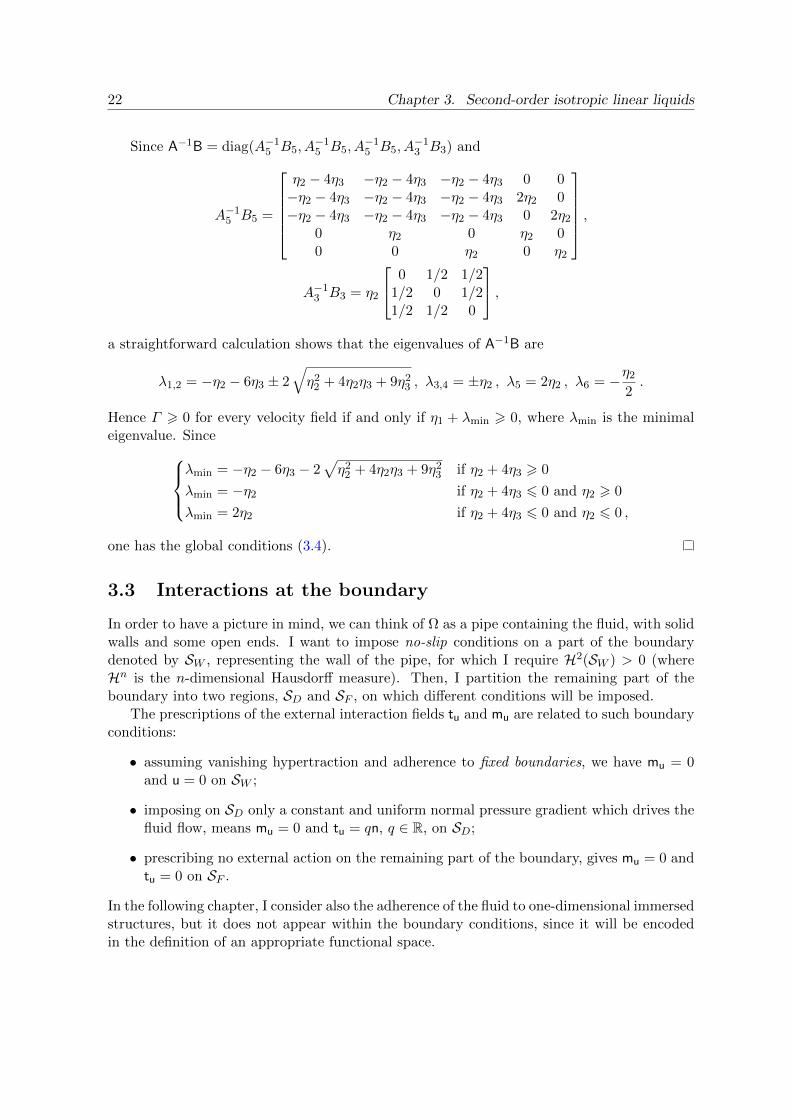
Since A−1B = diag(A−15 B5, A

−15 B5, A

−15 B5, A

−13 B3) and

A−15 B5 =

η2 − 4η3 −η2 − 4η3 −η2 − 4η3 0 0−η2 − 4η3 −η2 − 4η3 −η2 − 4η3 2η2 0−η2 − 4η3 −η2 − 4η3 −η2 − 4η3 0 2η2

0 η2 0 η2 00 0 η2 0 η2

,

A−13 B3 = η2

0 1/2 1/21/2 0 1/21/2 1/2 0

,a straightforward calculation shows that the eigenvalues of A−1B are

λ1,2 = −η2 − 6η3 ± 2√η2

2 + 4η2η3 + 9η23 , λ3,4 = ±η2 , λ5 = 2η2 , λ6 = −η2

2.

Hence Γ > 0 for every velocity field if and only if η1 + λmin > 0, where λmin is the minimaleigenvalue. Since

λmin = −η2 − 6η3 − 2√η2

2 + 4η2η3 + 9η23 if η2 + 4η3 > 0

λmin = −η2 if η2 + 4η3 6 0 and η2 > 0

λmin = 2η2 if η2 + 4η3 6 0 and η2 6 0 ,

one has the global conditions (3.4).

3.3 Interactions at the boundary

In order to have a picture in mind, we can think of Ω as a pipe containing the fluid, with solidwalls and some open ends. I want to impose no-slip conditions on a part of the boundarydenoted by SW , representing the wall of the pipe, for which I require H2(SW ) > 0 (whereHn is the n-dimensional Hausdorff measure). Then, I partition the remaining part of theboundary into two regions, SD and SF , on which different conditions will be imposed.

The prescriptions of the external interaction fields tu and mu are related to such boundaryconditions:

• assuming vanishing hypertraction and adherence to fixed boundaries, we have mu = 0and u = 0 on SW ;

• imposing on SD only a constant and uniform normal pressure gradient which drives thefluid flow, means mu = 0 and tu = qn, q ∈ R, on SD;

• prescribing no external action on the remaining part of the boundary, gives mu = 0 andtu = 0 on SF .

In the following chapter, I consider also the adherence of the fluid to one-dimensional immersedstructures, but it does not appear within the boundary conditions, since it will be encodedin the definition of an appropriate functional space.

Chapter 4

Analysis of the differential problems

I now want to investigate existence and uniqueness of solutions for both the stationary andthe evolutionary motion of a second-order incompressible fluid in a bounded Lipschitz domainΩ, in which a one-dimensional structure Λ is immersed. The assumption of the balanceprinciple (3.1) in integral form leads directly to an interpretation of the functions as definedup to negligible sets (with zero Lebesgue measure). Indeed, both the real velocity field u andthe virtual velocity v will belong to Hilbert spaces, whose definition is given in what follows.

4.1 The functional setting

We can construct a Hilbert subspace X of the Sobolev space H2(Ω;R3) in the following way:we set

V :=

v|Ω : v ∈ C∞0 (R3;R3) , div v = 0

and denote with H and H2d the completions of V in L2(Ω;R3) and H2(Ω;R3) respectively.

Since H2(Ω;R3) is continuously embedded in C0(Ω;R3), we can define in an obvious way theclosed subspace

Y :=

v ∈ H2(Ω;R3) : v = 0 on SW ∪ Λ

;

finally we set X := H2d ∩ Y endowed with the H2(Ω;R3) norm

‖v‖2X :=

∫Ω|v|2 +

∫Ω|∇v|2 +

∫Ω|∇∇v|2,

that encodes the natural regularity requested by the problem.It is apparent that velocity fields belonging to the space X vanish on SW ∪Λ (while their

derivatives in general do not); hence we can model adherence to walls and to one-dimensionalimmersed structures in a way consistent with the boundary conditions of Section 3.3. Itremains to specify the role of the time variable t, which clearly enters the problem via thetime derivative of u. As a first step we could take u ∈ L2([0, T ];X), so that u(t, ·) ∈ X foralmost every t ∈ [0, T ]; but we will see that, if u is a solution of our problem, then

u ∈ L2([0, T ];X) ∩ C0([0, T ];H) ∩H1([0, T ];X ′) =: X .

Given the representations of internal and external powers introduced in the previous chap-ter, the Principle of Virtual Powers, which corresponds to the equation of motion, becomesthe following statement.

23

24 Chapter 4. Analysis of the differential problems

Problem 1. Find u ∈ X such that

2µ

∫ T

0

∫Ω

Sym∇u · ∇v + (η1 − η2)

∫ T

0

∫Ω∇∇u · ∇∇v

+ 3η2

∫ T

0

∫Ω

Sym∇∇u · ∇∇v − (η2 + 4η3)

∫ T

0

∫Ω

∆u ·∆v∫ T

0

∫Ω

(∂u

∂t+ (u · ∇)u

)· v =

∫ T

0

∫SDqn · v +

∫ T

0

∫Ω

d · v , (4.1)

for every v ∈ X.

When stating the evolutionary problem, I will add an initial condition, while, to obtainthe stationary problem, it is enough to set the time derivative of u equal to zero, to erase thetime integrals, and to change X into X in the previous statement.

In equation (4.1) the only nonlinearity is the convective term (u · ∇)u ; clearly, it is thesource of the main difficulties in solving our problem. I will work it out via a topologicalmethod in which compactness is the key tool; therefore, let me introduce some considerationsabout the compactness properties of that term.

Consider the bilinear function

F :

H2 ×H2 → L2

(u, v) 7→ (u · ∇)v;

by Holder’s inequality, since H2(Ω;R3) is embedded in L∞(Ω;R3), we have(1)

‖F (u, v)‖L2 = ‖(u · ∇)v‖L2 6 ‖u‖L∞ ‖∇v‖L2 6 c0 ‖u‖H2 ‖v‖H2 (4.2)

for any u, v ∈ H2(Ω;R3); hence F is continuous.

Theorem 4.1. The Navier operator K0(u) := F (u, u) is compact from X to X ′.

Proof. As already noticed, the bilinear function F is continuous and so is K0, by compositionwith the function u 7→ (u, u) . Moreover, by virtue of (4.2), it is bounded on boundedsubsets of X.

Since X ⊆ H2(Ω;R3) is compactly embedded in L2(Ω;R3), we can identify L2(Ω;R3) withits dual space and apply Schauder’s theorem [5, Theorem 6.4] to obtain L2(Ω;R3) compactlyembedded in X ′.

Remark 4.1. The operator K0 is also compact from any W ⊆ H1(Ω) to W ′; in fact theimmersion H1(Ω)→ Lq(Ω) is compact for q ∈ [1, 6[ and such it is the dual Lq

′(Ω)→ (H1(Ω))′.

We can take q = 4, q′ = 43 , make the extension

F :

H1 ×H1 → L

43

(u, v) 7→ (u · ∇)v

and accordingly define K0 on W . We have

‖(u · ∇)v‖L

436 ‖u‖L4 ‖∇v‖L2 6 c0 ‖∇u‖L2 ‖∇v‖L2 < +∞

for any u, v ∈ W and, following the arguments of the previous theorem, we obtain the com-pactness of K0 from W to W ′. ♦

(1) Throughout this chapter ci, i ∈ N, denotes a positive constant depending only upon the geometry of Ω.

4.2. The stationary problem 25

When considering the evolutionary problem, we need K0 to be a compact operator fromL2([0, T ];X) into L2([0, T ];X ′). The following lemma, proved in [26, Chap. 1, Sec. 5.2], willbe useful.

Lemma 4.2. Given three Banach spaces B0 ⊂ B ⊂ B1 with B0 and B1 reflexive and B0

compactly embedded in B, and for T ∈ (0,+∞) and p0, p1 ∈ (1,+∞) fixed, set

W :=

v : v ∈ Lp0([0, T ];B0) ,

∂v

∂t∈ Lp1([0, T ];B1)

.

Then W is a Banach space compactly embedded in Lp0([0, T ];B).

Theorem 4.3. The Navier operator K0 is compact from the space

X = L2([0, T ];X) ∩ C0([0, T ];H) ∩H1([0, T ];X ′)

into L2([0, T ];X ′).

Proof. Since X is compactly embedded in L3(Ω;R3) and so is L32 (Ω;R3) into X ′, we can

apply Lemma 4.2 with X ⊂ L3(Ω;R3) ⊂ X ′ and p0 = p1 = 2. It remains to show that K0, as

an operator with range in L2([0, T ];L32 (Ω;R3)), is bounded on bounded subsets of its domain.

The estimate ∫ T

0‖F (u, v)‖2

L32dt 6

∫ T

0‖∇v‖2L6 ‖u‖2L2 6 c2

1

∫ T

0‖v‖2H2 ‖u‖2L2

gives the needed property since u belongs to L∞([0, T ];H).

4.2 The stationary problem

I will first solve the stationary version of Problem 1, in which time dependence is suppressed.Stationary solutions represent an important class in Fluid Mechanics for many applications;moreover, the treatment of the evolutionary problem follows a similar argument.

Let us define the bilinear form a : X ×X → R as follows:

a(u, v) := 2µ

∫Ω

Sym∇u · ∇v + (η1 − η2)

∫Ω∇∇u · ∇∇v

+ 3η2

∫Ω

Sym∇∇u · ∇∇v − (η2 + 4η3)

∫Ω

∆u ·∆v .

In view of the dissipation inequality (3.3) and Proposition 3.1, I will assume a slightly strongerhypothesis on the sign of the coefficients.

Proposition 4.4. Provided that

µ > 0 , η1 + 2η2 > 0 , η1 − η2 > 0 , η1 − η2 − 6η3 − 2√η2

2 + 4η2η3 + 9η23 > 0 ,

the bilinear form a(u, v) is continuous and coercive on X.


Proof. The continuity of a is apparent. With the notation of Proposition 3.1, we have:

a(u, u) = 2µ

∫Ω|Sym∇u|2 +

∫ΩΓ > 2µ ‖Sym∇u‖2L2 + (η1 + λmin) ‖∇∇u‖2L2 ;

by an application of Korn’s inequality [22, Lemma 6.2], there exists κ > 0 such that

a(u, u) > κ(‖u‖2L2 + ‖∇u‖2L2) + (η1 + λmin) ‖∇∇u‖2L2 .

Setting

ν := min κ , η1 + λmin > 0 ,

we have a(u, u) > ν ‖u‖2X .

Consider now the trilinear form b : H2 ×H2 ×H2 → R given by

b(u, v,w) :=

∫ΩF (u, v) · w =

∫Ω

(u · ∇)v · w ,

which is indeed continuous since

|b(u, v,w)| 6 ‖F (u, v)‖L2 ‖w‖L2 6 c0 ‖u‖H2 ‖v‖H2 ‖w‖H2

for every u, v,w ∈ H2(Ω;R3).

Lemma 4.5. For every u ∈ X we have b(u, u, u) = 0 .

Proof. By standard formulae in tensor calculus we get the assertion for u ∈ V and we canextend it by a density argument.

In the course of the proof of the existence result for solutions of the stationary problem,also the following theorem [9, Corollary 8.1] will be applied.

Theorem (Fixed Point). Let X be a Banach space and Φ : X → X a compact operator.Then either Φ(u) = u has a solution, or the set

S =

u ∈ X : Φ(u) = λu for some λ > 1

is unbounded.

Theorem 4.6. There exists u ∈ X such that, for every v ∈ X,

a(u, v) + b(u, u, v) = 〈ϕ, v 〉 , (4.3)

where ϕ ∈ X ′ is the linear form defined by

〈ϕ, v 〉 =

∫SDqn · v +

∫Ω

d · v .

4.3. The evolutionary problem 27

Proof. By the Lax-Milgram theorem, the function L : X → X ′ defined by

∀v ∈ X : 〈L(u), v 〉 = a(u, v)

is a homeomorphism. We have

L(u) +K0(u) = ϕ in X ′ (4.4)

and then

u = L−1 (ϕ−K0(u)) =: Φ(u).

Assume that u ∈ X is a solution of (4.4); it means that for every v ∈ X

〈L(u), v 〉+ 〈K0(u), v 〉 = 〈ϕ, v 〉.

Taking v = u and applying Lemma 4.5, we can write

ν ‖u‖2X 6 a(u, u) 6 |b(u, u, u)|+ |〈ϕ, u 〉| 6 ‖ϕ‖X′ ‖u‖X ;

from which we have the a priori estimate

‖u‖X 61

ν‖ϕ‖X′ =: R < +∞ . (4.5)

Take now λ > 1 and assume that Φ(u) = λu; it means that

〈L(λu), u 〉+ 〈K0(u), u 〉 = 〈ϕ, u 〉

and, following the argument leading to (4.5), we obtain ‖u‖X 6 λ−1R < R .

Hence the set S introduced in the Fixed Point theorem is bounded and there exists afixed point u ∈ X for Φ. We can then conclude that such u is a stationary solution forProblem 1.

Remark 4.2. Considering the Sobolev constant c0 introduced in (4.2), it is easy to prove that,if the condition c0 ‖ϕ‖X′ < ν2 is satisfied, then the solution of the stationary problem isunique. This condition resembles that of a low Reynolds number: indeed it entails also theexponential stability of the unique stationary solution of the evolutionary problem treatedbelow. ♦

4.3 The evolutionary problem

I now come to analyze the evolutionary problem. Take u ∈ L2([0, T ];X), whose norm is

‖u‖2L2([0,T ];X) :=

∫ T

0‖u(s)‖2X ds ,

and take ϕ ∈ L2([0, T ];X ′) defined by

〈ϕ, v 〉 =

∫ T

0

∫SDqn · v +

∫ T

0

∫Ω

d · v .


Theorem 4.7. For every u0 ∈ H there exists u ∈ L2([0, T ];X) such that

u(0) = u0, (4.6)∫ T

0

(∫Ω

∂u

∂t· v + a(u, v) + b(u, u, v)

)= 〈ϕ, v 〉, (4.7)

for every v ∈ L2([0, T ];X).

Remark 4.3. Notice that the time derivative of u has to be interpreted as a linear formin L2([0, T ];X ′), whose representation enters equation (4.7), and thus we will take u ∈H1([0, T ];X ′). A key role in the evolutionary problem is played by the initial datum u0

which belongs to H. At first the initial condition (4.6) should be understood in X ′, but wewill see that it actually holds in H, as u belongs to C0([0, T ];H). After these considerationswe can take u ∈ X. ♦

Proof. In order to proceed we need some estimates; first we set v = u in (4.7) and applyLemma 4.5 obtaining that ∫

Ω

∂u

∂t· u + a(u, u) = 〈ϕ, u 〉

for almost every t ∈ [0, T ]. Integrating in time we get:

1

2

∫ t

0

d

ds‖u(s)‖2L2 ds+

∫ t

0a(u, u) ds =

∫ t

0〈ϕ, u 〉 ds ;

hence, applying also Young’s inequality,

1

2‖u(t)‖2L2 + ν

∫ t

0‖u‖2X ds 6

1

2‖u0‖2L2 +

ν

2

∫ t

0‖u‖2X ds+ c2

∫ t

0‖ϕ‖2X′ ds ,

that gives the first estimate for a.e. t ∈ [0, T ]:

‖u(t)‖2L2 + ν

∫ t

0‖u‖2X ds 6 ‖u0‖2L2 + 2c2

∫ t

0‖ϕ‖2X′ ds =: M .

This a priori bound tells us that any solution u of our problem belongs to a bounded subsetof L2([0, T ];X) ∩ L∞([0, T ];H). We now need the following theorem whose proof is givenin [27, Chap. 3, Sec. 4.4].

Theorem (J. L. Lions). Let X and H be two Hilbert spaces, with X dense and continuouslyembedded in H; identify H with its dual in such a way that X ⊂ H ⊂ X ′ and fix T > 0.Consider a bilinear form at(u, v) : X ×X → R such that:

i) the function t 7→ at(u, v) is measurable for every u, v ∈ X ;

ii) |at(u, v)| 6 C1 ‖u‖X ‖v‖X for a.e. t ∈ [0, T ], for every u, v ∈ X;

iii) at(v, v) > α ‖v‖2X − C2 ‖v‖2H for a.e. t ∈ [0, T ], for every v ∈ X;

where α > 0, C1 and C2 are constants.Then, for every f ∈ L2([0, T ];X ′) and for every u0 ∈ H, there exists only one u such that

u ∈ L2([0, T ];X) ∩ C0([0, T ];H) ∩H1([0, T ];X ′)

u(0) = u0

〈 ∂u

∂t(t), v 〉+ at(u(t), v) = 〈 f(t), v 〉 for a.e. t ∈ [0, T ], for every v ∈ X.

4.3. The evolutionary problem 29

It is easy to see that the spaces X, H and the bilinear form at(u, v) := a(u(t), v(t)) fulfillthe hypotheses of the previous theorem; then the function

L :

X → H × L2([0, T ];X ′)

u 7→(

u(0),∂u

∂t(t) + a(u(t), · )

)is a homeomorphism.

We can now write equations (4.6)–(4.7) in H × L2([0, T ];X ′) as

L(u) + ( 0 , K0(u) ) = ( u0 , ϕ ),

from which

u = L−1( u0 , ϕ−K0(u) ) =: Φ(u).

By Theorem 4.3 and composition arguments, Φ turns out to be a compact operator, and wecan then apply the Fixed Point theorem in the Banach space X. Arguing as in the previoussection, we take λ > 1 and assume Φ(u) = λu; in particular u0 = λu(0) and

λ

2

∫ t

0

d

ds‖u(s)‖2L2 ds+ λ

∫ t

0a(u, u) ds =

∫ t

0〈ϕ, u 〉 ds .

We then obtain

λ

2‖u(t)‖2L2 + λν

∫ t

0‖u‖2X ds 6

λ

2

∥∥λ−1u0

∥∥2

L2 +ν

2

∫ t

0‖u‖2X ds+ c2

∫ t

0‖ϕ‖2X′ ds ,

that gives

λ ‖u(t)‖2L2 + (2λ− 1)ν

∫ t

0‖u‖2X ds 6 λ−1 ‖u0‖2L2 + 2c2

∫ t

0‖ϕ‖2X′ ds < M .

Since 2λ− 1 > λ, we can write

‖u(t)‖2L2 + ν

∫ t

0‖u‖2X ds < λ−1M

and the set S in the Fixed Point theorem is bounded in L2([0, T ];X)∩L∞([0, T ];H). In orderto complete the proof, it remains to show that S is bounded also in H1([0, T ];X ′).

If there exists λ > 1 such that Φ(u) = λu, then we have that

∂u

∂t= −a(u, · )− 1

λK0(u) +

1

λϕ in L2([0, T ];X ′)

and that ∥∥∥∥∂u

∂t

∥∥∥∥X′

6 ‖a(u, · )‖X′ +1

λ‖K0(u)‖X′ +

1

λ‖ϕ‖X′ .

By the continuity of a and the embeddings mentioned in the proof of Theorem 4.3 we canwrite: ∥∥∥∥∂u

∂t

∥∥∥∥X′

6 c3 ‖u‖X +c4

λ‖K0(u)‖

L32

+1

λ‖ϕ‖X′ .


We know that u belongs to a bounded subset of L2([0, T ];X) and ϕ ∈ L2([0, T ];X ′); wededuce that ∫ T

0

∥∥∥∥∂u

∂t

∥∥∥∥2

X′6 c5 +

2c24

λ2

∫ T

0‖K0(u)‖2

L32< N

for a fixed N > 0, since K0 maps bounded subsets of L2([0, T ];X)∩L∞([0, T ];H) to bounded

subsets of L2([0, T ];L32 (Ω;R3)).

The last bound shows that ∂u∂t belongs to a bounded subset of L2([0, T ];X ′) and implies

that S is bounded in X. Hence there exists a fixed point u ∈ X for Φ and this is a solutionfor the Cauchy problem (4.6)–(4.7).

Thanks to the H2-regularity of the solution we have found, which in particular guaranteesthe L∞-regularity in three dimensions, an important uniqueness result can be proved.

Theorem 4.8. There exists a unique solution u ∈ X of the Cauchy problem (4.6)–(4.7).

Proof. Let u1 and u2 be solutions of equation (4.7) with the same initial datum and setw := u1 − u2. We easily obtain, by equations (4.6)–(4.7) and Lemma 4.5,

w(0) = 0,∫Ω

∂w

∂t· w + a(w,w) + b(w, u2,w) = 0 ,

from which, integrating in time and applying the coercivity of a, we can deduce that

1

2‖w(t)‖2L2 + ν

∫ t

0‖w‖2X ds 6

∫ t

0|b(w, u2,w)| ds .

By Young’s inequality,

‖w(t)‖2L2 + 2ν

∫ t

0‖w‖2X ds 6 2

∫ t

0‖w‖L∞ ‖∇u2‖L2 ‖w‖L2 ds

6 2c0

∫ t

0‖w‖X ‖u2‖X ‖w‖L2 ds 6 2ν

∫ t

0‖w‖2X ds+

c20

2ν

∫ t

0‖u2‖2X ‖w‖

2L2 ds ;

hence we have

‖w(t)‖2L2 6c2

0

2ν

∫ t

0‖u2(s)‖2X ‖w(s)‖2L2 ds

and by Gronwall’s lemma we conclude that ‖w(t)‖2L2 = 0 for every t ∈ [0, T ], that is u1 =u2.

Remark 4.4. Notice that, if η1 = η2 = 0 and η3 < 0, the bilinear form a is no longer coerciveon X; nevertheless, all the previous results are still valid, if we replace X with the space

X := v ∈ completion of V in H1(Ω;R3) : ∆v ∈ L2(Ω;R3) and v = 0 on SW ∪ Λ ,

on which the bilinear form a remains coercive, a key feature for existence theorems.Moreover, standard regularity theorems for elliptic second-order PDEs, guarantee that

functions belonging to X are essentially bounded [14, Theorem 8.16] and Holder continuous[14, Theorem 8.22]. Essential boundedness provides the needed estimates for uniqueness ofthe solution, while the continuity in space of the solutions allows to assign their value on aone-dimensional set contained in the interior of Ω. ♦

4.4. Immersed structures dragging the fluid 31

4.4 Immersed structures dragging the fluid

I now want to study the flow of a second-gradient linear liquid dragged by one-dimensionalimmersed structures in an arbitrary time interval [0, T ] when the three-dimensional regionoccupied by the fluid Ω is a bounded domain with Lipschitz boundary which is fixed in time.Since here the emphasis is on the drag, I impose the boundary conditions stated in Section 3.3,with SW = ∂Ω. For the sake of simplicity I consider only one rigid body Λ0 immersed in thefluid, where Λ0 is a connected one-dimensional closed subset of Ω such that Λ0 ∩ ∂Ω = ∅.Moreover, I denote by Λ(t) the image at time t of Λ0 under the rigid displacement ϕ, i.e.Λ(t) = ϕ(Λ0, t) and Λ(0) = Λ0. I assume the existence of a family of C2-diffeomorphismsψt : Ω→ Ω such that ψt(Λ0) = Λ(t) and any ψt reduces to the identity map in a neighborhoodof ∂Ω. This assumption will be fulfilled if the one-dimensional structure never reaches theboundary of the domain, namely Λ(t) ∩ ∂Ω = ∅ for every t ∈ [0, T ]. Finally, to avoidtechnicalities, I assume that ϕ and ψt enjoy a C1 dependence on time. The introduction ofsuch diffeomorphisms will enable us to map the linearized parabolic problem with a movingdomain into an equivalent problem, easier to work out, where Λ(t) = Λ0 for all the time.

I construct, for every t ∈ [0, T ], a Hilbert subspace Xt of the Sobolev space H2(Ω;R3) inthe following way: recall that I set

V :=

v|Ω : v ∈ C∞0 (R3;R3) , div v = 0

(4.8)

and denote with H and H2d the completions of V in L2(Ω;R3) and H2(Ω;R3) respectively.

Since H2(Ω;R3) is continuously embedded in C0(Ω;R3), we can define the closed subspace

Xt :=

v ∈ H2(Ω;R3) : v = 0 on ∂Ω ∪ Λ(t)∩H2

d (4.9)

endowed with the H2-norm.Now I can redefine the space

X := L2([0, T ];Xt) ∩ C0([0, T ];H) ∩H1([0, T ];X ′t) (4.10)

of divergence-free virtual velocities on Ω which belong to Xt for almost every t ∈ [0, T ], andwhose first derivatives with respect to t belong to the dual space X ′t of Xt for a.e. t ∈ [0, T ].Moreover, it is apparent that velocity fields belonging to the space X vanish on [0, T ] × ∂Ωand on the surface (t, x) : t ∈ [0, T ], x ∈ Λ(t) .

Consider again the continuous bilinear form on H2(Ω;R3) defined by

at(u, v) := 2µ

∫Ω

Sym∇u · ∇v

+ (η1 − η2)

∫Ω∇∇u · ∇∇v + 3η2

∫Ω

Sym∇∇u · ∇∇v

− (η2 + 4η3)

∫Ω

∆u ·∆v . (4.11)

Since at(u, u) represents the dissipation at time t of the flow u, the classical Korn’s inequalitytogether with the constraints (3.4) on the coefficients (taken with strict inequalities) guaranteethe coercivity of this bilinear form on the space Xt.

In order to prove the existence of a solution for the dynamical problem, assume to havean interpolator u, namely a divergence-free velocity field which vanishes on ∂Ω and equals the


velocity of the rigid body on Λ(t), and to look for a solution of the type u + u where u ∈ X.Then, substituting into the balance (3.1) and using the properties of u, it is straightforwardto see that u must satisfy the following problem.

Problem 2. Given u0 ∈ H and u as above, find u ∈ X such that u|t=0 = u0 and∫ T

0

(∫Ω

∂u

∂t· v + at(u, v)

)+

∫ T

0(b(u, u, v) + b(u, u, v) + b(u, u, v))

+

∫ T

0

(∫Ω

∂u

∂t· v + at(u, v) + b(u, u, v)

)= 0 (4.12)

for every v ∈ X.

In order to show that Problem 2 has a solution u ∈ X (and that it is the sole one), I needa further “smallness” condition on the interpolator u, that is, for a suitable β > 0,

|b(v, u, v)| 6 β ‖v‖2H2 , (4.13)

which we suppose, for the time being, to be fulfilled. The problem of finding an interpolatorwill be considered in a while.

Now I will solve Problem 2. The first step is to define the linearized parabolic operator

L :

X → H × L2([0, T ];X ′t)

u 7→(

u|t=0 ,∂u

∂t(t) + at(u(t), · )

)(4.14)

and to establish that it is a homeomorphism. This fact guarantees that, at least when theconvective term can be neglected (e.g. in the case of low Reynolds numbers), the problemadmits a unique solution. Such a result can be obtained by the same argument used in theprevious section, once we have noticed that the time-varying spaces Xt turn all into X0 whenwe apply ψ−1

t to Ω, and the coercivity of the bilinear form at is transferred to a new bilinearform a, as explained in [25]. After this transformation, we obtain a parabolic problem on thedomain (t, ψ−1

t (x)) : t ∈ [0, T ], x ∈ Ω , which enjoys existence and uniqueness of solution inthe space

L2([0, T ];X0) ∩ C0([0, T ];H) ∩H1([0, T ];X ′0) ; (4.15)

hence L is a homeomorphism.As a second step, one has to deal with the nonlinear term K(u) := (u · ∇)u. Its com-

pactness properties have been successfully exploited in the previous sections and, since thesame arguments apply also here, we need no additional effort to establish the existence of asolution u ∈ X for Problem 2. Uniqueness follows again by the proof of Theorem 4.8.

The construction of a good interpolator u is not trivial, because in order to prove theexistence of solutions we need a family of interpolators of the velocity assigned on Λ(t) and∂Ω among which, for any β > 0, a u can be selected such that (4.13) holds for every v ∈ Xt.In order to obtain a divergence-free interpolator g(t, x), we consider, at any fixed time t, aneighborhood Rt ⊂ Ω of Λ(t) with ∂Rt smooth. On Rt the field g is taken equal to thevelocity of the rigid motion ϕ; since this is a divergence-free velocity and since we want g tovanish on ∂Ω, we get ∫

∂(Ω\Rt)g · n =

∫∂Ω

g · n−∫∂Rt

g · n = 0 , (4.16)

4.4. Immersed structures dragging the fluid 33

where n is the outer unit normal to ∂(Ω \ Rt). The existence of such a g is granted by thefollowing lemma, which can be easily proved, adapting the argument in [15, Lemma 2.2].

Lemma 4.9. Let A be an open connected subset of R3. For each g ∈ H32 (∂A;R3) satisfying∫

∂Ag · n = 0 ,

there exists a function g ∈ H2(A;R3) such that div g = 0 in A and g = g on ∂A.

Carefully considering what happens on ∂Rt, it turns out that the function

h :=

ϕ on Rt

g on Ω \Rt

belongs to H2(Ω;R3). Once h is found, we can construct u satisfying (4.13) via two steps: wetake Rt small enough, and then we apply Lemma 7.1 of [26, p. 103] on Ω \ Rt thanks to theregularity of ∂Rt.

Chapter 5

The role of higher-order materialparameters

The aim of this chapter is to analyze the effects of the higher-order material parameters η1, η2,η3 in some examples, in order to gain some insight into their meaning both from a physicaland a mathematical point of view. It will become clear that η1 is strictly related to thepresence of concentrated interactions, while η3 is only responsible for higher-order dissipationphenomena. The role of η2 is less clear.

5.1 Dragged flow in a cylinder

Consider a fluid placed in the cavity between two infinitely long coaxial cylinders of radiiR1 < R2; the flow is driven imposing a motion with constant velocity U of the inner cylinderalong the axial direction ez. Looking for cylindrically symmetric stationary solutions u(r)ez,where r is the cylindrical radius, in the case of Newtonian liquids with viscosity µ and theusual adherence condition on the walls, one easily finds

u(r) = UlogR2 − log r

logR2 − logR1. (5.1)

It is clear that this solution has no continuous extension to the case R1 = 0.However, with a second-order linear isotropic viscous liquid the analogous problem gives

the family of solutions

u(r) = α1 + α2I0

( rL

)+ α3 log

( rL

)+ α4K0

( rL

), (5.2)

where αi, i = 1 . . . 4, are constants (depending on R1, R2) fixed by the boundary conditions,I0, K0 are Bessel functions of imaginary argument [24, Sec. 5.7], and the parameter

L :=√

(η1 − η2 − 4η3)/µ (5.3)

arises from the higher-oreder terms. If we now set R1 = 0 the solution remains boundedprovided that α3 = α4, since

limr→0

(log( rL

)+K0

( rL

))< +∞ ; (5.4)

34

5.1. Dragged flow in a cylinder 35

ex

ey

Figure 5.1: Section of the cylindrical sector.

besides, one can still meet the prescribed boundary conditions by a suitable choice of theconstants.

Actually, true boundary conditions can now be imposed only at r = R2, while, at r = 0,I will impose the value of the velocity field to be equal to U . This is an example of theconstraint on the space of velocities which is considered in the previous chapter. Hence, beingn the outer unit normal to the cylinder, the three conditions are:

u(0) = U , (5.5)

u(R2) = 0 , (5.6)

(Gn)n|r=R2 = 0 . (5.7)

While the first two conditions are clear and do not contain explicitly the higher-order param-eters, condition (5.7) has to be specialized. On the surface of the cylinder we have

(Gn)n = η1∂2u

∂r2− (η2 + 4η3)

1

r

∂

∂r

(r∂u

∂r

)which implies [

η1∂2u

∂r2− (η2 + 4η3)

1

r

∂

∂r

(r∂u

∂r

)]r=R2

= 0 . (5.8)

Now, recall that the thermodynamical constraints (3.4) force η2 to vanish if η1 = 0, whileη3 can be any non-positive real number. On the other hand, in order to prove Proposition 4.4,η1 cannot vanish, but if this is the case, with η3 < 0, the fluid is still a non-simple one,thermodynamics is not violated, and we still have a unique solution according to Remark 4.4.

So far there is no clear distinction between the effects of the presence of the three pa-rameters. Let us now calculate the concentrated force on the edges of a π/2-wide cylindricalsector, whose section is depicted in Fig. 5.1. Given the geometry, we have to evaluate theconcentrated traction on the edges; with the notation of Proposition 2.4, we get

Ku = G(ex ⊗ ey + ey ⊗ ex) = 2G(ex ⊗ ey) ;

indeed

G112 = G212 = 0 , and G312 = η1∂2u

∂x∂y.

36 Chapter 5. The role of higher-order material parameters

0.00080 0.0002 0.0004 0.0006 0.0010150

160

170

180

190

200

210

220

Second-gradient flow rate vs L

Newtonian flow rate vs R1

length L or R1 (cm)

flowrate(cm

3/s)

Figure 5.2: Comparison of the flow rates.

Hence it is clear that the parameter η3 does not play any role in the determination of theconcentrated force Ku. Moreover, if η1 = 0, no concentrated force can appear.

This result is in agreement with the general feature discussed in Section 2.2, and theresults in [31, Sec. 4]. Indeed, the hyperstress takes the form

G = −5η3∆u⊗ I + 3η3 Sym(∆u⊗ I) + I⊗ p ,

whose active part, given the incompressibility constraint, is G0 = −4η3∆u ⊗ I, which, byCorollary 2.6, cannot develop concentrated interactions.

Remark 5.1. The results of the present section show that the adherence to a one-dimensionalobject should not be viewed as a concentrated interaction; indeed, we can constitutivelychoose to have a fluid which can interact with one-dimensional objects without developingconcentrated stresses. This is in fact the case when η1 = η2 = 0 and η3 < 0, and thatsituation corresponds to the particular choice, introduced in Remark 4.4, of the functionalspace to which our velocity field belong.

Such a result is a bit surprising. But we have to properly understand the meaning ofconcentrated interactions; in fact, what we get in the case η1 = η2 = 0, η3 < 0 is that the ad-herence to a one-dimensional structure can be represented, on any material surface containingit, by diffused surface interactions. On the other hand, when η1 > 0, the representation ofinternal stresses can have a concentrated part on the singular edges of the surface of somesubbody, even though there are no concentrated interactions on any part of the boundary orthe interior of the whole body. ♦

As to the meaning of the length-scale L, an interesting feature appears. Computing thedependence upon R1 of the flow rate through an annular section in the Newtonian case, andcomparing it with the dependence upon L of the flow rate of our second-gradient fluid whenthe inner radius is equal to zero (Fig. 5.2), one can observe that the relative difference between

5.2. Pressure-driven flows 37

the two values computed at R1 = L is very small, indeed negligible when R1, L 1. Thisfact suggests that the parameter L represents a sort of effective thickness in the limiting case.

5.2 Pressure-driven flows

I will finally describe analytic expressions for the pressure-driven flow of a second-order liquidin a pipe with squared or circular section.

Consider a pipe with squared section in the (x, y)-plane, a velocity field v = w(x, y)ez, anda constant and uniform pressure gradient Cez whic drives the flow. The differential equationfor the steady flow of a second-order liquid with viscosity µ, becomes

µ∆w − ξ∆∆w = C , (5.9)

with w = 0 and ∂2w∂n2 = 0 on the boundary of the pipe. Notice that ∆ is the bidimensional

Laplace operator in the (x, y)-plane. The previous equation can be written as

−∆(w − L2∆w) = −Cµ, L2 :=

ξ

µ,

and, since w − L2∆w = 0 on the boundary, we can set u = w − L2∆w, obtaining−∆u = −C/µ =: C

u = 0 on the boundary.(5.10)

Take now the section of the pipe to be [0, π]× [0, π], so that we can expand on the basis givenby the eigenfunctions of the Laplace operator on that square:

Xh,k =4

π2sinhx sin ky,

with eigenvalues λh,k = h2 + k2, with h, k ∈ N. We have

〈C,Xh,k〉 =

fh,k := 8C

π2 hk for h, k odd

0 otherwise.

Hence the solution of (5.10) is

u =∑

h,k odd

fh,kλh,k

Xh,k. (5.11)

It remains to solve−L2∆w + w = u .

The operator (−L2∆ + 1) has again Xh,k as eigenfunctions, with eigenvalues L2λh,k + 1; thenwe get

w(x, y) =∑

h,k odd

fh,kλh,k(L2λh,k + 1)

Xh,k =

= −32C

µπ4

∑h,k odd

hk

(h2 + k2)(L2h2 + L2k2 + 1)sinhx sin ky . (5.12)

38 Chapter 5. The role of higher-order material parameters

Now we can evaluate the concentrated traction along the edges of the pipe. As in theprevious section we have

Ku = 2G(ex ⊗ ey) ;

and

G112 = G212 = 0 , G312 = η1∂2w

∂x∂y.

Once more, we see that a concentrated stress can appear only if η1 > 0, while a second-orderliquid with η1 = 0 cannot develop such a concentration even if the boundary of the domainhas a singular part.

Let us compute, with η1 > 0, the concentrated stress density in the origin:

Ku(0, 0) = 2η1∂2w

∂x∂y(0, 0)ez = −2η1

32C

µπ4

∑h,k odd

h2k2

(h2 + k2)(L2h2 + L2k2 + 1)ez 6= 0 .

Thanks to the symmetry of the problem, we get the same result on the remaining edges.Take now an incompressible fluid which moves in a cylindrical pipe of radius R; the motion

is again produced imposing a uniform pressure gradient Cez (C ∈ R) on the z = 0 circularsection, being the axis of the cylinder along the z direction ez. Looking for cylindricallysymmetric stationary solutions u(r)ez, where r2 = x2 + y2, in the case of Newtonian liquidswith viscosity µ and the usual adherence condition, one finds

u(r) =C

4µ(r2 −R2)

for the axial component of the velocity field.With a second-order fluid the analogous problem gives the family of solutions

u(r) =C

4µr2 + α1 + α2I0

( rL

)+ α3 log r + α4K0

( rL

),

where, as in the previous section, αi, i = 1 . . . 4, are constants fixed by the boundary condi-tions, L is the length-scale arising from the higher-order terms and I0, K0 are Bessel functions.Regularity assumptions for r = 0 imply α3 = α4 = 0, and the boundary conditions become

u(R) = 0 , (5.13)

(Gn)n|r=R = 0 , (5.14)

that is

C

4µR2 + α1 + α2I0

(R

L

)= 0 , (5.15)

(η1 − η2 − 4η3)

(α2

2L2

[I0

(R

L

)+ I2

(R

L

)])− (η2 + 4η3)

(C

µ+α2

LRI1

(R

L

))= 0 , (5.16)

from which

α1 = − C4µR2 − α2I0

(R

L

), (5.17)

α2 =C

µ

η2 + 4η3η1−η2−4η3

2L2

[I0

(RL

)+ I2

(RL

)]− η2+4η3

LR I1

(RL

) . (5.18)

Since the modified Bessel functions In grow exponentially fast, we see that, when L is smallcompared to the radius R of the cylinder, the second-order solution is very similar to theclassical one.

Appendix A

Differentiable Banach manifolds

Within the present section I collected basic definitions and properties of Banach manifolds,which essentially are differentiable manifolds whose local charts are isomorphic to an opensubset of a Banach space, not necessarily of Rn, so that the more familiar theory of differ-entiable manifolds is recovered as a particular case. For a complete treatment of the subjectthe reader is referred to [23] and [1].

Definition A.1. Let S be a set. A chart on S is a bijection ϕ from a subset U of S to anopen subset of a Banach space. We sometimes denote ϕ by (U,ϕ), to indicate the domain Uof ϕ. A Ck atlas on S is a family of charts A = (Ui, ϕi) : i ∈ I such that:

(i) S =⋃i∈I Ui ;

(i) Any two charts in A are compatible in the sense that the overlap maps between membersof A are Ck diffeomorphisms: for any two charts (Ui, ϕi) and (Uj , ϕj) with Ui ∩ Uj 6=∅, we define the overlap map on the intersection as ϕji := ϕi ϕ−1

j , and we require

ϕi(Ui ∩ Uj) to be open and ϕji to be a Ck diffeomorphisms.

Definition A.2. Two Ck atlases A1 and A2 are equivalent if A1 ∪ A2 is a Ck atlas. A Ck

differentiable structure D on S is an equivalence class of atlases on S. The union of the atlasesin D,

AD :=⋃A : A ∈ D

is the maximal atlas of D, and a chart (U,ϕ) ∈ AD is an admissible local chart.A differentiable manifold M is a pair (S,D), where S is a set and D is a Ck differentiable

structure on S. If a covering by charts takes values in a Banach space B, then B is called themodel space and we say that M is a Ck Banach manifold modeled on B.

It is now clear that any Banach space B is a Banach manifold, whose differentiable struc-ture is given by the atlas with the sole identity chart.

Definition A.3. Let (S1,D1) and (S2,D2) be two manifolds. The product manifold

(S1 × S2,D1 ×D2)

consists of the set S1 × S2 together with the differentiable structure D1 × D2 generated bythe atlas

(U1 × U2, ϕ1 × ϕ2) : (Ui, ϕi) is a chart of (Si,Di), i = 1, 2 .

39

40 Appendix A. Differentiable Banach manifolds

Definition A.4. Let M be a manifold and m ∈ M . A curve at m is a C1 map c : I → Mfrom an interval I ⊆ R into M with 0 ∈ I and c(0) = m. Let c1 and c2 be two curves at mand (U,ϕ) an admissible chart with m ∈ U . Then we say c1 and c2 are tangent at m withrespect to ϕ if and only if (ϕ c1)′(0) = (ϕ c2)′(0).

Proposition A.1. Let c1 and c2 be two curves at m ∈ M . Suppose (Ui, ϕi) are admissiblecharts with m ∈ Ui, i = 1, 2. Then c1 and c2 are tangent at m with respect to ϕ1 if and onlyif they are tangent at m with respect to ϕ2.

By the previous proposition, tangency at m ∈M is an equivalence relation among curvesat m, and an equivalence class with respect to tangency at m of such curves will be denotedby [ c ]m, where c is a representative of the class.

Definition A.5. For a manifold M and m ∈M the tangent space to M at m is

TmM := [ c ]m : c is a curve at m ;

given A ⊆M we set

TM |A :=⋃m∈A

TmM ,

and TM := TM |M is the tangent bundle on M . The mapping τM : TM → M , defined byτM ([ c ]m) = m, is the tangent bundle projection on M .

Proposition A.2. Let U be an open subset of the Banach space B, and let c be a curve atu ∈ U . Then there is a unique b ∈ B such that the curve cu,b defined by cu,b(t) = u+ tb (witht belonging to an interval I such that cu,b(I) ⊂ U) is tangent to c at u.

In particular TU can be identified with U×B, and TuU is isomorphic to B for any u ∈ U .

Proof. By definition, the differential Dc(0) is the unique linear map from R to B such thatthe curve g : R → B, given by g(t) = u + tDc(0) is tangent to c at t = 0. If b = Dc(0),then g = cu,b. Hence, the map i : U × B → TU defined by i(u, b) = [ cu,b ]u, turns out tobe a bijection; moreover, we can induce a manifold structure on TU by means of i, and thisconcludes the proof.

I will now define cotangent spaces and bundles in the particular case which is of interestwithin the present work.

Definition A.6. Let U be an open subset of the Banach space B. Then, for any u ∈ U , thetopological dual of TuU ∼= B defines the cotangent space at u, denoted by T ∗uU , and

T ∗U :=⋃u∈U

T ∗uU

is the cotangent bundle on U .

Appendix B

Differential operators on a surface

Given a smooth surface S embedded in R3, we can define the projection operator P on S,and its composition with the gradient and the divergence operator. Let n be the unit outernormal to S; for any vector field a and any tensor field A, we have:

P := I− n⊗ n ,

∇S a := (∇a)P ,

divS a := tr(∇S a) = P · ∇a = div a− n · (∇a)n ,

(divS A)i := Aij,kPkj ,

where tr(A) denotes the trace of the matrix A. Moreover, the normal derivative is defined as

∂a

∂n:= (∇a)n ;

the curvature tensor C(x) and the mean curvature k(x) of S are defined by

C(x) := −∇S n = −(∇n)P ,

k(x) :=1

2tr C = −1

2divS n .

for any x ∈ S.With these definitions we have the following important result.

Surface-divergence Theorem B.1. Let τ be a vector field tangent to S, and let U ⊆ S bea subsurface with ν unit outer normal to ∂U ; then∫

∂Uτ · ν =

∫U

divS τ . (B.1)

By direct application of the previous theorem to suitable tangential fields, we get thefollowing corollary.

Corollary B.2. For any tensor field A, any vector field a and any virtual velocity v, we have:

divS(AP) = divS A + 2kAn , (B.2)

divS(A†a) = a · divS A + A · ∇S a , (B.3)∫S

A · ∇S v = −∫S

(divS A + 2kAn) · v . (B.4)

41

Bibliography

[1] R. Abraham, J. E. Marsden, and T. Ratiu. Manifolds, tensor analysis, and applications,volume 75 of Applied Mathematical Sciences. Springer-Verlag, New York, second edition,1988.

[2] R. A. Adams and J. J. F. Fournier. Sobolev spaces, volume 140 of Pure and AppliedMathematics (Amsterdam). Elsevier/Academic Press, Amsterdam, second edition, 2003.

[3] S. S. Antman and J. E. Osborn. The principle of virtual work and integral laws of motion.Arch. Rational Mech. Anal., 69(3):231–262, 1979.

[4] J. M. Ball. Convexity conditions and existence theorems in nonlinear elasticity. Arch.Rational Mech. Anal., 63(4):337–403, 1976/77.

[5] H. Brezis. Functional analysis, Sobolev spaces and partial differential equations. Univer-sitext. Springer, New York, 2011.

[6] B. D. Coleman and W. Noll. The thermodynamics of elastic materials with heat con-duction and viscosity. Arch. Rational Mech. Anal., 13:167–178, 1963.

[7] B. Dacorogna. Direct methods in the calculus of variations, volume 78 of Applied Math-ematical Sciences. Springer-Verlag, Berlin, 1989.

[8] M. Degiovanni, A. Marzocchi, and A. Musesti. Edge-force densities and second-orderpowers. Ann. Mat. Pura Appl. (4), 185(1):81–103, 2006.

[9] K. Deimling. Nonlinear functional analysis. Springer-Verlag, Berlin, 1985.

[10] E. Feireisl. On the motion of a viscous, compressible, and heat conducting fluid. IndianaUniv. Math. J., 53(6):1705–1738, 2004.

[11] M. Fremond. Non-smooth thermomechanics. Springer-Verlag, Berlin, 2002.

[12] E. Fried and M. E. Gurtin. Tractions, balances, and boundary conditions for nonsimplematerials with application to liquid flow at small-length scales. Arch. Ration. Mech.Anal., 182(3):513–554, 2006.

[13] P. Germain. La methode des puissances virtuelles en mecanique des milieux continus. I.Theorie du second gradient. J. Mecanique, 12:235–274, 1973.

[14] D. Gilbarg and N. S. Trudinger. Elliptic partial differential equations of second order.Classics in Mathematics. Springer-Verlag, Berlin, 2001. Reprint of the 1998 edition.

42

Bibliography 43

[15] V. Girault and P.-A. Raviart. Finite element methods for Navier-Stokes equations, vol-ume 5 of Springer Series in Computational Mathematics. Springer-Verlag, Berlin, 1986.Theory and algorithms.

[16] G. Giusteri, A. Marzocchi, and A. Musesti. Three-dimensional nonsimple viscous liquidsdragged by one-dimensional immersed bodies. Mechanics Research Communications,37(7):642–646, 2010.

[17] G. Giusteri, A. Marzocchi, and A. Musesti. Nonsimple isotropic incompressible linearfluids surrounding one-dimensional structures. Acta Mechanica, 217:191–204, 2011.

[18] M. E. Gurtin. A gradient theory of single-crystal viscoplasticity that accounts for geo-metrically necessary dislocations. J. Mech. Phys. Solids, 50(1):5–32, 2002.

[19] M. E. Gurtin, E. Fried, and L. Anand. The Mechanics and Thermodynamics of Continua.Cambridge University Press, New York, 2010.

[20] P. Haj lasz. Sobolev spaces on metric-measure spaces. In Heat kernels and analysis onmanifolds, graphs, and metric spaces (Paris, 2002), volume 338 of Contemp. Math.,pages 173–218. Amer. Math. Soc., Providence, RI, 2003.

[21] J. Heinonen. Nonsmooth calculus. Bull. Amer. Math. Soc. (N.S.), 44(2):163–232, 2007.

[22] N. Kikuchi and J. T. Oden. Contact problems in elasticity: a study of variational in-equalities and finite element methods, volume 8 of SIAM Studies in Applied Mathematics.Society for Industrial and Applied Mathematics (SIAM), Philadelphia, PA, 1988.

[23] S. Lang. Differential manifolds. Springer-Verlag, New York, second edition, 1985.

[24] N. N. Lebedev. Special functions and their applications. Dover Publications Inc., NewYork, 1972. Revised edition, translated from the Russian and edited by Richard A.Silverman, Unabridged and corrected republication.

[25] J. Lımaco, L. A. Medeiros, and E. Zuazua. Existence, uniqueness and controllability forparabolic equations in non-cylindrical domains. Mat. Contemp., 23:49–70, 2002. SeventhWorkshop on Partial Differential Equations, Part II (Rio de Janeiro, 2001).

[26] J.-L. Lions. Quelques methodes de resolution des problemes aux limites non lineaires.Dunod, Paris, 1969.

[27] J.-L. Lions and E. Magenes. Problemes aux limites non homogenes et applications. Vol.1. Travaux et Recherches Mathematiques, No. 17. Dunod, Paris, 1968.

[28] A. Musesti. Isotropic linear constitutive relations for nonsimple fluids. Acta Mech.,204(1):81–88, 2009.

[29] D. O’Regan, Y. J. Cho, and Y.-Q. Chen. Topological degree theory and applications,volume 10 of Series in Mathematical Analysis and Applications. Chapman & Hall/CRC,Boca Raton, FL, 2006.

[30] P. Podio-Guidugli. A virtual power format for thermomechanics. Contin. Mech. Ther-modyn., 20(8):479–487, 2009.

44 Bibliography

[31] P. Podio-Guidugli and M. Vianello. Hypertractions and hyperstresses convey the samemechanical information. Contin. Mech. Thermodyn., 22(3):163–176, 2010.

[32] R. A. Toupin. Elastic materials with couple-stresses. Arch. Rational Mech. Anal., 11:385–414, 1962.

[33] W. P. Ziemer. Weakly differentiable functions. Sobolev spaces and functions of boundedvariation, volume 120 of Graduate Texts in Mathematics. Springer-Verlag, New York,1989.

Higher-gradient Theories for Fluids and Concentrated E ects

Documents

Transcript of Higher-gradient Theories for Fluids and Concentrated E ects