HIGH SPEED TWO (HS2) LIMITEDassets.hs2.org.uk/sites/default/files/inserts/HS2 Regional...
95
September 2013 Ref: HS2/074 HIGH SPEED TWO (HS2) LIMITED HS2 Regional Economic Impacts
Transcript of HIGH SPEED TWO (HS2) LIMITEDassets.hs2.org.uk/sites/default/files/inserts/HS2 Regional...
September 2013 Ref: HS2/074
HIGH SPEED TWO (HS2) LIMITEDHS2 Regional Economic Impacts
HIGH SPEED TWO (HS2) LIMITEDHS2 Regional Economic Impacts
September 2013

A report prepared for High Speed Two (HS2) Limited:
High Speed Two (HS2) Limited has been tasked by the Department for Transport (DfT) with managing the delivery of a new national high speed rail network. It is a non-departmental public body wholly owned by the DfT.
High Speed Two (HS2) Limited,2nd Floor, Eland House,Bressenden Place,London SW1E 5DU
Telephone: 020 7944 4908
General email enquiries: [email protected]
Website: www.hs2.org.uk
This document is issued for the party which commissioned it and for specific purposes connected with the captioned project only. It should not be relied upon by any other party or used for any other purpose.
We accept no responsibility for the consequences of this document being relied upon by any other party, or being used for any other purpose, or containing any error or omission which is due to an error or omission in data supplied to us by other parties.
Underlying maps in this report sourced from Ordnance Survey © Crown copyright and database right 2013. Licence available at http://www.ordnancesurvey.co.uk/docs/licences/os-opendata-licence.pdf
Ref: HS2/074
Printed in Great Britain on paper containing at least 75% recycled fibre.

HS2 Regional Economic Impact | Contents
i
High Speed Two (HS2) Limited HS2 Regional Economic Impacts
Ref: HS2 / 074
September 2013

HS2 Regional Economic Impact | Contents
ii
Notice: about this report
This report has been prepared by KPMG LLP on behalf of High Speed Two Limited (HS2 Ltd), in accordance with the terms of KPMG LLP’s engagement with HS2 Ltd, exclusively for the benefit of HS2 Ltd. This report is not suitable to be relied on by any other party wishing to acquire rights against KPMG LLP for any purpose or in any context. Any party other than HS2 Ltd that obtains access to this report or a copy (under the Freedom of Information Act 2000, through HS2 Ltd’s Publication Scheme, or otherwise) and chooses to rely on it (or any part of it) does so at its own risk. To the fullest extent permitted by law, KPMG LLP does not assume any responsibility and will not accept any liability in respect of this report to any party other than HS2 Ltd.
In particular, and without limiting the general statement above, since KPMG LLP has prepared this report for the benefit of HS2 Ltd, it has not been prepared for the benefit of any other person or organisation that might have an interest in the matters discussed in this report. Nothing in this report constitutes a valuation, audit or legal advice.
The information in this report is based upon publicly available information and information provided to KPMG LLP by HS2 Ltd. It reflects prevailing conditions and views as of this date, all of which are accordingly subject to change. In preparing this report, KPMG LLP have relied upon and assumed, without independent verification, the accuracy and completeness of the information upon which the report is based, including that available from public sources and that provided by third parties.
The analysis undertaken by KPMG LLP contains commercially valuable methodologies that are proprietary to KPMG LLP. The projections set out in the analysis have been prepared for illustrative purposes only and do not constitute a forecast. Whilst KPMG LLP has undertaken the analysis in good faith, no warranty, expressed or implied, is made in respect of the accuracy, completeness or appropriateness of its assumptions, calculations or results. No reliance may be placed upon the analysis by any party, except where specifically referred to in an agreed KPMG LLP letter of engagement. All users are accordingly advised to undertake their own analysis and due diligence before making any decision or entering into any commitment based on the information in this report.

HS2 Regional Economic Impact | Contents
iii
Contents
Executive Summary 7
1 Introduction 16
1.1 Background 16
1.2 Purpose of this report 17
1.3 HS2 service pattern and released capacity 19
1.4 Structure of this report 22
2 HS2 and the city region economies 23
2.1 Potential impacts 23
3 Methodological approaches 28
3.1 Background to development 28
3.2 Analytical approaches 29
4 Methodology to estimate the economic impacts of investment in HS2 33
4.1 Building an approach 33
4.2 Measuring connectivity 35
4.3 Productivity impacts 40
4.4 Business location impacts 43
4.5 Overview of productivity and business location analysis 45
4.6 Areas for further analysis 46
5 Results 50
5.1 Productivity impacts for the British economy 50
5.2 Distribution of economic output after business location effects 53
5.3 Summary of potential impacts 56
6 Technical appendices 58
6.1 Key assumptions and data inputs 58
6.2 Calculating connectivity 62
6.3 Productivity and business location analysis 72
List of figures
Figure 1: Estimated changes in rail business-to-business connectivity in 2037 after investment in HS2 10
Figure 2: Estimated changes in economic output after investment in HS2 (2037, at 2013 prices) 14
Figure 3: City region descriptions 19
Figure 4: Estimated changes in rail business-to-business connectivity in 2037 after investment in HS2 22
Figure 5: Categorisation of potential impacts 23
Figure 6: Why the connectivity of a business location matters 24
Figure 7: Illustration of the production function 25
Figure 8: Interaction between business impacts and people impacts 27
HS2 Regional Economic Impact | Contents
iv
Figure 9: Alternative analytical approaches 31
Figure 10: Illustrative example decay curve 37
Figure 11: Decay curves derived for rail and car by journey purpose (2010) 38
Figure 12: Illustration of business connectivity 39
Figure 13: Analytical process to calibrate productivity and business location analysis 45
Figure 14: Analytical process to forecast ranges for future economic outcomes 46
Figure 15: Potential distribution of economic output in 2037 after investment in HS2 54
Figure 16: Estimated changes in economic output after investment in HS2 (2037, at 2013 prices) 56
Figure 17: Map of PLANET Long Distance model zones 63
Figure 18: Decay curves derived for rail and car trips by journey purpose (2010) 69
Figure 19: Impact of different logit scale parameters on modelled GDP impacts in the Phase Two city regions 91
List of tables
Table 1: Average change in connectivity by region in 2037 after investment in HS2 9
Table 2: Total annual productivity impacts for Great Britain in 2037 after investment in HS2 (2013 prices) 13
Table 3: Average change in connectivity by city region in 2037 after investment in HS2 20
Table 4: Estimated elasticities of productivity with respect to connectivity 42
Table 5: Areas for further analysis and implications for current work 46
Table 6: Total annual productivity impacts for Great Britain in 2037 after investment in HS2 (2013 prices) 50
Table 7: Total annual productivity impacts for Great Britain by source of connectivity in 2037 after investment in HS2 (2013 prices) 50
Table 8: Total annual productivity impacts for Great Britain by source of connectivity in 2037 after investment in HS2 (2013 prices), using a mode share approach to weighting the relative importance of connectivity for productivity 52
Table 9: Total annual productivity impacts for Great Britain in 2037 after investment in HS2 (2013 prices) when assuming half the value of in-vehicle time for business users 53
Table 10: Estimated changes in economic output by city region in 2037 after investment in HS2 (2013 prices) 55
Table 11: Complete list of data sources used in the analysis 60
Table 12: Variables extracted from the PLANET Long Distance model used for the calculation of generalised costs 65
Table 13: Generalised Cost Parameters (2002 Prices and Values) 67
Table 14: Econometric analysis of different connectivity measures for the construction sector, 2010 76
Table 15: Econometric analysis of different connectivity measures for the consumer services sector, 2010 77
Table 16: Econometric analysis of different connectivity measures for the manufacturing sector, 2010 78
Table 17: Econometric analysis of different connectivity measures for the producer services sector, 2010 79
Table 18: Elasticities of productivity with respect to measures of connectivity with quality adjusted labour 81
Table 19: Production function model coefficients 84
Table 20: Production function model coefficients 85

HS2 Regional Economic Impact | Contents
v
Table 21: UK data on production and transport costs, £m, 2010 89
Table 22: Estimated business trips per £ of output 90
Table 23: HS2 services pattern and re-deployment of classic network capacity assumed in the August 2012 economic case 91

HS2 Regional Economic Impact | Introduction
7
Executive summary HS2 is the largest expansion of Britain’s rail network since the Victorian era. It will provide additional rail capacity, substantially reduce journey times and improve connectivity between markets.
KPMG is working on behalf of HS2 Ltd to develop a methodological framework to analyse the potential scale, range and distribution of regional economic impacts associated with the substantial improvements to the rail network brought about by HS2 and the used of freed-up capacity on the classic rail network. In undertaking this work, KPMG has been assisted by Connected Economics Limited.
The project has been peer-reviewed by an advisory panel of independent experts set up by HS2 Ltd to provide advice on the scope, design and delivery of an analytical work programme to explore the potential impact of investment in HS2 on the economy1.
This document provides a summary of the methodology and results of the analysis. It is based on data and assumptions for the full HS2 network (i.e. following completion of both Phase One and
Phase Two) and the associated re-deployment of classic network capacity that were used to support the latest economic case for HS2, published in August 20122. The analysis therefore addresses the potential impacts of the full HS2 network, rather than separately assessing the impacts associated with Phases One and Two.
Throughout the remainder of this Executive Summary, when we refer to investment in HS2, this should be read as investment in the full HS2 network and the associated reorganisation and use of capacity on the classic rail network.
The design of HS2, the associated re-deployment of classic network capacity, and the
methodology used to assess regional economic impacts continue to be developed and refined. The work presented here should therefore be considered the first step in assessing the scheme’s potential impact on the economy. It is anticipated that forecast impacts will be updated as the broader programme of work develops.
The work considers how patterns of economic activity vary across alternative markets and geographies, and how these differences relate to differences in levels of transport connectivity between businesses and labour markets. The analysis then examines how investment in HS2 could affect connectivity and, ultimately, economic output, drawing on empirical analysis of current travel patterns and observed relationships between connectivity and economic growth.
The analysis focuses on the potential impact of investment in HS2 on the structure of regional economies in the longer term. It is therefore different from conventional approaches to the
appraisal of transport schemes, which are based on the estimation of the monetary value of travel time and cost changes.
1 We are grateful to the Advisory panel for their input to the project, but note that the views expressed in this document are entirely those of the authors 2 HS2 Ltd (2012) Updated Economic Case for HS2 http://assets.hs2.org.uk/sites/default/files/inserts/Updated%20economic%20case%20for%20HS2.pdf
HS2 Regional Economic Impact | Introduction
8
Although the analysis draws on some of the same inputs as conventional appraisal methods, it
does not seek to value travel time and cost changes directly. Instead, it aims to understand how these changes to travel times and costs influence regional economic performance, both in terms of overall economic productivity and the location of economic activity. The analysis provides an alternative approach to conventional transport appraisal and the estimated net benefits should not be considered as comparable or additional to those estimated by conventional appraisal techniques. The approach is also different from that used to estimate potential employment and regeneration impacts immediately around the planned HS2 stations, as it considers the net impacts on economic output for city regions and the economy as a whole.
HS2 service pattern and released capacity
As noted above, the analysis is based on data and assumptions used to support the August 2012 iteration of the economic case3. These do not include the Manchester Airport High Speed Station
but do include the Heathrow spur. However, in January 2013 the Government announced that it was pausing work on the spur to Heathrow pending the outcome of the work of the Airports Commission, chaired by Sir Howard Davies. The initial preferred route for Phase Two that is currently out to consultation does include a high speed rail station at Manchester Airport.
The HS2 scheme assessed includes 18 high speed trains per hour in each direction on the southern route into and out of Euston, of which broadly half are wholly contained on high speed infrastructure and half run on to the classic network4. The scheme also includes a major re-design of services on a significant proportion of the classic rail network, using the additional capacity released by HS2 to enhance frequency, connectivity and capacity on the classic network.
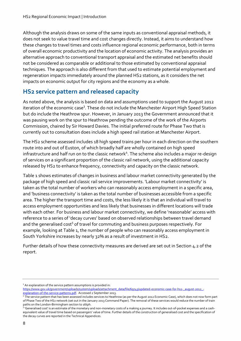
Table 1 shows estimates of changes in business and labour market connectivity generated by the package of high speed and classic rail service improvements. 'Labour market connectivity' is taken as the total number of workers who can reasonably access employment in a specific area,
and 'business connectivity' is taken as the total number of businesses accessible from a specific area. The higher the transport time and costs, the less likely it is that an individual will travel to access employment opportunities and less likely that businesses in different locations will trade with each other. For business and labour market connectivity, we define ‘reasonable’ access with reference to a series of ‘decay curves’ based on observed relationships between travel demand and the generalised cost5 of travel for commuting and business purposes respectively. For example, looking at Table 1, the number of people who can reasonably access employment in South Yorkshire increases by nearly 32% as a result of investment in HS2.
Further details of how these connectivity measures are derived are set out in Section 4.2 of the report.
3 An explanation of the service pattern assumptions is provided in: https://www.gov.uk/government/uploads/system/uploads/attachment_data/file/69743/updated-economic-case-for-hs2-_august-2012_-explanation-of-the-service-patterns.pdf. Accessed 2 September 2013. 4 The service pattern that has been assessed includes services to Heathrow (as per the August 2012 Economic Case), which does not now form part of Phase Two of the HS2 network (set out in the January 2013 Command Paper). The removal of these services would reduce the number of train paths on the London-Birmingham section to 16tph. 5 'Generalised cost' is an estimate of the monetary and non-monetary costs of a making a journey. It includes out-of-pocket expenses and a cash-equivalent value of travel time based on passengers’ value of time. Further details of the construction of generalised cost and the specification of the decay curves are reported in the Technical Appendices.
HS2 Regional Economic Impact | Introduction
9
Table 1: Average change in connectivity by region in 2037 after investment in HS2
City regions Change in labour connectivity by rail Change in business connectivity by rail
Derby-Nottingham 14.7% 23.2%
Greater Manchester 1.4% 18.8%
Greater London 6.9% 8.8%
South Yorkshire 31.8% 22.5%
West Midlands 15.7% 21.1%
West Yorkshire 9.1% 19.7%
Rest of Great Britain 5.3% 11.3%
Notes: (1) The estimates show the GDP-weighted improvement in rail connectivity for the model zones within the defined geographies (i.e. the zones comprising the city regions and the zones comprising the rest of Great Britain). (2) The estimates are based on train timetable assumptions used in the August 2012 economic case for HS2.
Our analysis shows that widespread improvements in rail connectivity are experienced across Great Britain after investment in HS2, particularly for business-to-business markets, which increase for every area of Great Britain assessed. This reflects the use of significant freed-up capacity on the classic rail network that is brought about by the introduction of HS2. Figure 1 below shows the scale of rail business-to-business connectivity changes in 2037.
HS2 Regional Economic Impact | Introduction
10
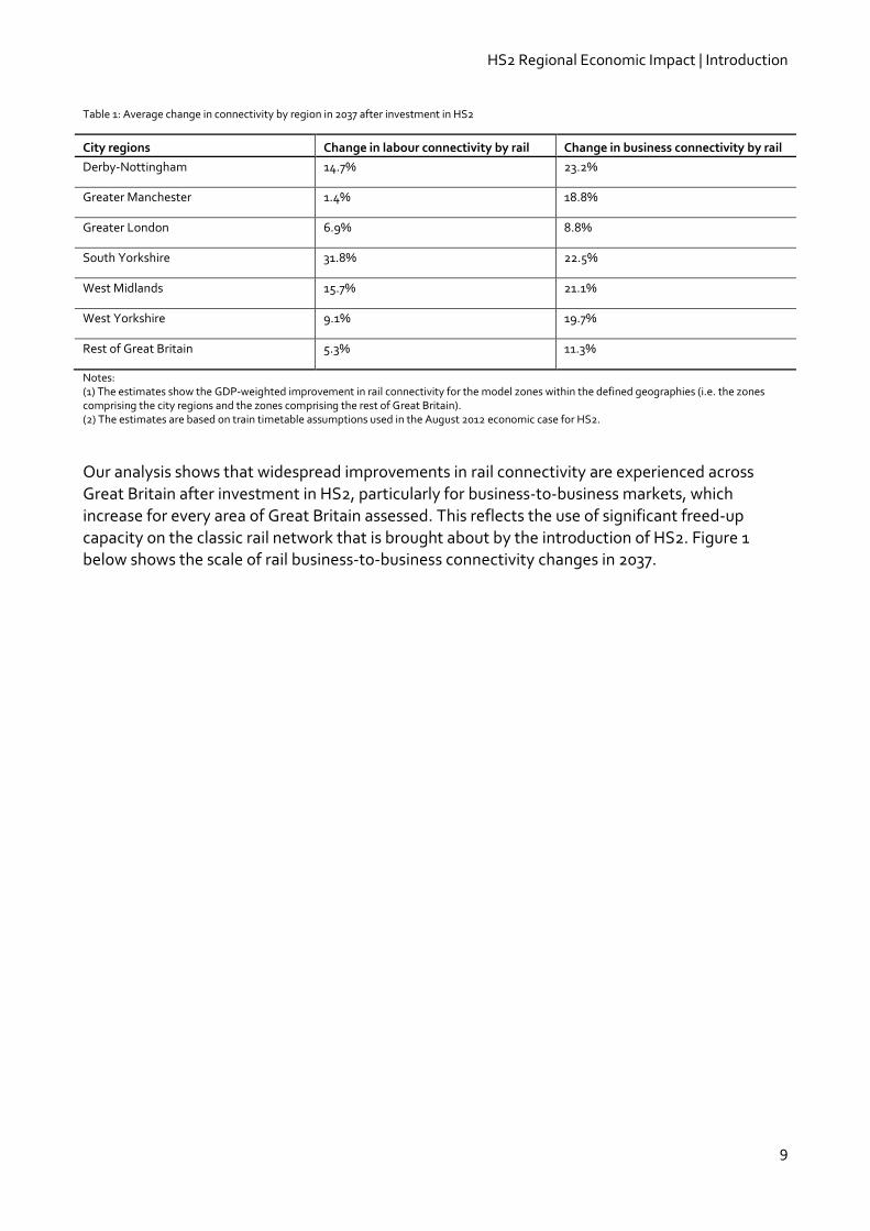
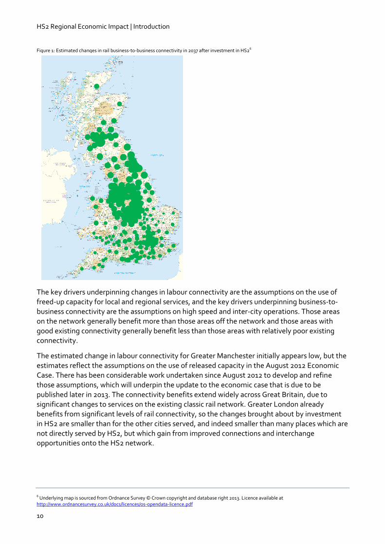
Figure 1: Estimated changes in rail business-to-business connectivity in 2037 after investment in HS26
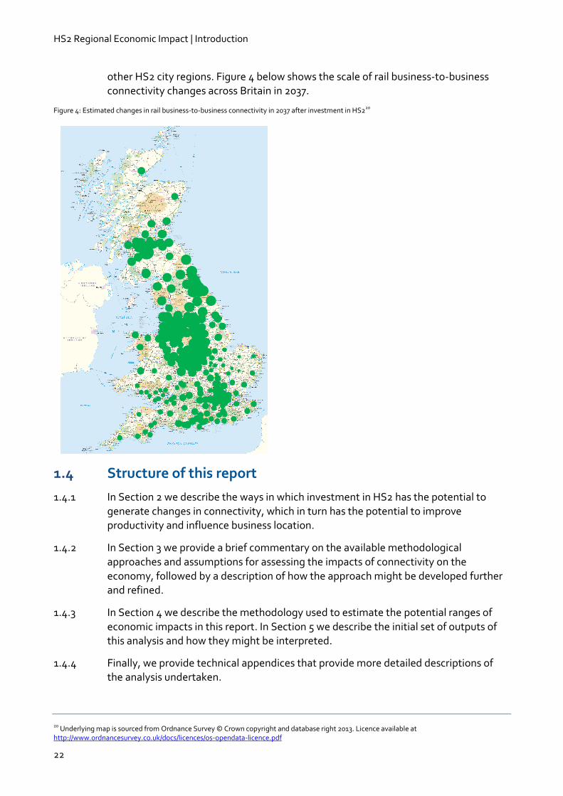
The key drivers underpinning changes in labour connectivity are the assumptions on the use of
freed-up capacity for local and regional services, and the key drivers underpinning business-to-business connectivity are the assumptions on high speed and inter-city operations. Those areas on the network generally benefit more than those areas off the network and those areas with good existing connectivity generally benefit less than those areas with relatively poor existing connectivity.
The estimated change in labour connectivity for Greater Manchester initially appears low, but the estimates reflect the assumptions on the use of released capacity in the August 2012 Economic Case. There has been considerable work undertaken since August 2012 to develop and refine those assumptions, which will underpin the update to the economic case that is due to be published later in 2013. The connectivity benefits extend widely across Great Britain, due to significant changes to services on the existing classic rail network. Greater London already benefits from significant levels of rail connectivity, so the changes brought about by investment
in HS2 are smaller than for the other cities served, and indeed smaller than many places which are not directly served by HS2, but which gain from improved connections and interchange opportunities onto the HS2 network.
6 Underlying map is sourced from Ordnance Survey © Crown copyright and database right 2013. Licence available at http://www.ordnancesurvey.co.uk/docs/licences/os-opendata-licence.pdf
HS2 Regional Economic Impact | Introduction
11
HS2 and the city region economies
We consider the following factors to be important to our understanding of the link between rail infrastructure investment, improved connectivity and economic performance. Reduced transport costs following infrastructure investments will:
enable businesses to serve markets further afield and be more competitive in markets that they currently serve;
enable businesses to more easily connect with potential suppliers, allowing them to access inputs of higher quality and/or lower cost;
provide consumers with improved access to a wider range of suppliers, offering quality improvements and/or lower prices; and
improve the functioning of the labour market, increasing the effective size of
the market and allowing skills to be better matched to employment opportunities.
The reduced transport costs reduce barriers to trade, enabling markets to function more efficiently, stimulating competition and driving improvements in productivity. Those areas that are better connected will benefit from larger ‘effective market sizes’, leading to economies of agglomeration and increased specialisation, which in turn generate productivity gains over and above the transport cost efficiencies.
Methodology to estimate regional economic impacts
Investment in HS2 has the potential to affect the functioning of the labour market, business productivity and competitiveness. These impacts interact over time and can lead to changes in economic output and the spatial distribution of economic activity.
We have developed a practical and transparent methodology to quantify the economic impact of
investment in HS2. Our approach makes use of data and assumptions assembled to support the August 2012 economic case for HS2.
This approach builds on KPMG’s previous work in this area7, considering the relationship between transport connectivity and economic output, but undertaking a more fine-grained analysis of how additional economic output is redistributed, on the basis of production cost advantages arising from economies of agglomeration together with transport cost advantages.
The two aspects of the approach are described further below.
Enhanced productivity
Changes in transport connectivity driven by increased capacity and reduced journey times can enable improved levels of economic productivity through:
7 KPMG for Greengauge 21 (2010) High Speed Rail in Britain: Consequences for employment and economic growth, as well as a number of unpublished studies, including work for several city regions across the UK to support the development of their local infrastructure investment programmes.
HS2 Regional Economic Impact | Introduction
12
specialisation of labour and specialisation within supply chains;
matching of skills to jobs, and suppliers to customers;
sharing of inputs with a minimum efficient scale; and
learning through knowledge spill-overs from denser economic agglomerations8.
To address productivity impacts, we have specified and estimated a ‘production function’ showing the relationship between economic output and inputs to the production process (labour and capital). Differences in transport connectivity affect production efficiencies and total output for a given level of input. The production function is calibrated to observed patterns of economic output and inputs for Great Britain in 2010.
Business location effects
Business and employment location changes result from:
changes in production costs; and
changes in the cost of transport which influence the costs of trade between areas.
To assess these impacts, we have developed an approach that addresses how productivity and connectivity changes have the potential to affect the competitiveness of businesses located in the city regions and elsewhere, as a result of changes in production and transport costs. Both affect the market share of businesses serving different locations and both have the potential to change the geographical distribution of economic activity.
The analysis uses data from HS2 Ltd’s assessment of the direct transport impacts of the scheme as reflected in the PLANET Long Distance (PLD) Model, which considers rail and car travel between 235 different geographic zones9. A map of these zones is provided in Section 6.2 of the technical appendices. The analysis necessarily assumes no economic benefits from trips within the same zone, and only captures impacts on passenger journeys. It therefore excludes the potential benefits associated with local journeys (by rail and other public transport), with enhanced freight capacity, and with improvements to the UK’s competitive position globally.
The approach considers the impact of changes to rail and car connectivity by journey purpose (business or commuting) on four sectors of the economy, which are:
construction;
consumer services (hospitality, land, retail, transport and wholesale services);
manufacturing; and
producer services (financial, insurance, IT and other business services).
8 Duranton, G. and Puga, D. (2003) Micro-foundations for Urban Agglomeration Economies, NBER Working Paper No. 9931 9 The PLANET Modelling Framework is a suite of transport models used by HS2 Ltd to represent the time, cost and demand of travel between origin and destinations (represented as model zones) across Great Britain using different service pattern scenarios. The PLANET Long Distance model forms part of this modelling framework. Further information on PLANET Long Distance is publicly available through HS2 Ltd’s website.
HS2 Regional Economic Impact | Introduction
13
These sectors cover around two-thirds of economic activity in Great Britain and exclude those
considered unlikely to benefit from investment in HS2 (e.g. agriculture). The results suggest that 95% of the forecast productivity gains arise in producer and consumer services.
Range of regional economic impacts
We have assessed the potential impact of investment in HS2 on the GB and regional economies in terms of the marginal increase in overall productivity and the change in geographical distribution of total output.
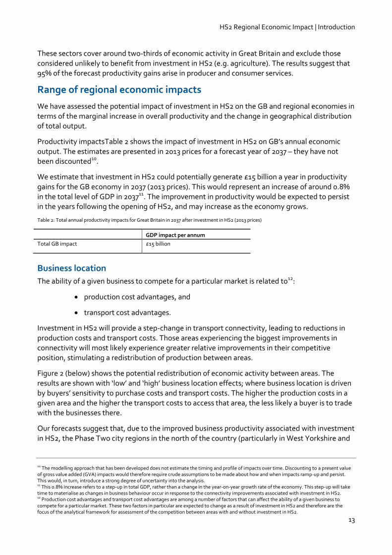
Productivity impactsTable 2 shows the impact of investment in HS2 on GB’s annual economic output. The estimates are presented in 2013 prices for a forecast year of 2037 – they have not been discounted10.
We estimate that investment in HS2 could potentially generate £15 billion a year in productivity
gains for the GB economy in 2037 (2013 prices). This would represent an increase of around 0.8% in the total level of GDP in 203711. The improvement in productivity would be expected to persist in the years following the opening of HS2, and may increase as the economy grows.
Table 2: Total annual productivity impacts for Great Britain in 2037 after investment in HS2 (2013 prices)
GDP impact per annum
Total GB impact £15 billion
Business location
The ability of a given business to compete for a particular market is related to12:
production cost advantages, and
transport cost advantages.
Investment in HS2 will provide a step-change in transport connectivity, leading to reductions in
production costs and transport costs. Those areas experiencing the biggest improvements in connectivity will most likely experience greater relative improvements in their competitive position, stimulating a redistribution of production between areas.
Figure 2 (below) shows the potential redistribution of economic activity between areas. The results are shown with ‘low’ and ‘high’ business location effects; where business location is driven by buyers’ sensitivity to purchase costs and transport costs. The higher the production costs in a given area and the higher the transport costs to access that area, the less likely a buyer is to trade with the businesses there.
Our forecasts suggest that, due to the improved business productivity associated with investment
in HS2, the Phase Two city regions in the north of the country (particularly in West Yorkshire and
10 The modelling approach that has been developed does not estimate the timing and profile of impacts over time. Discounting to a present value of gross value added (GVA) impacts would therefore require crude assumptions to be made about how and when impacts ramp-up and persist. This would, in turn, introduce a strong degree of uncertainty into the analysis. 11 This 0.8% increase refers to a step-up in total GDP, rather than a change in the year-on-year growth rate of the economy. This step-up will take time to materialise as changes in business behaviour occur in response to the connectivity improvements associated with investment in HS2. 12 Production cost advantages and transport cost advantages are among a number of factors that can affect the ability of a given business to compete for a particular market. These two factors in particular are expected to change as a result of investment in HS2 and therefore are the focus of the analytical framework for assessment of the competition between areas with and without investment in HS2.
HS2 Regional Economic Impact | Introduction
14
South Yorkshire), and even more so in the midlands (i.e. Derby-Nottingham and the West
Midlands), will experience an improvement in their competitive position relative to Greater London and the rest of Great Britain.
While there is more uncertainty in the pattern of business location effects after investment in HS2, we estimate that, of the total £15 billion additional output per year for the GB economy, between £5.5 billion and £7.8 billion of output per year could be generated in the Phase Two city regions outside Greater London.
While it is forecast that businesses relocate to those areas on, or well connected to, the Phase Two network, there are also widespread output gains well beyond the Phase Two city regions. Greater London and the rest of the country still experience material increases in economic output as businesses are forecast to become more productive as a result of investment in HS2.
In particular for the rest of Great Britain (i.e. outside of Greater London and the Phase Two city
regions), the forecast productivity gains are significant, even after the effects of business location. These productivity gains - estimated to be worth between £5 billion and £7 billion a year – are largely brought about by the use of freed-up capacity, which results in widespread improvements to rail services on the classic network, particularly on long-distance routes.
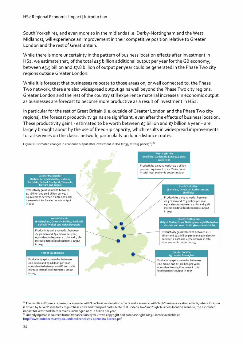
Figure 2: Estimated changes in economic output after investment in HS2 (2037, at 2013 prices) 13, 14
13 The results in Figure 2 represent a scenario with ‘low’ business location effects and a scenario with ‘high’ business location effects; where location is driven by buyers’ sensitivity to purchase costs and transport costs. Note that under a 'low' and 'high' business location scenario, the estimated impact for West Yorkshire remains unchanged at £1.0 billion per year. 14 Underlying map is sourced from Ordnance Survey © Crown copyright and database right 2013. Licence available at http://www.ordnancesurvey.co.uk/docs/licences/os-opendata-licence.pdf
Greater Manchester(Bolton, Bury, Manchester, Oldham,
Rochdale, Salford, Stockport, Tameside, Trafford and Wigan)
Productivity gains valued at between £1.3 billion and £0.6 billion per year; equivalent to between a 1.7% and 0.8% increase in total local economic output in 2037
West Yorkshire(Bradford, Calderdale, Kirklees, Leeds,
Wakefield)
Productivity gains valued at £1.0 billion per year; equivalent to a 1.6% increase in total local economic output in 2037
South Yorkshire(Barnsley, Doncaster, Rotherham and
Sheffield)
Productivity gains valued at between
£0.5 billion and £0.9 billion per year; equivalent to between a 1.9% and 3.2% increase in total local economic output in 2037
Derby-Nottingham(City of Derby, City of Nottingham, eight Derbyshire
districts and seven Nottinghamshire districts)
Productivity gains valued at between £1.1
billion and £2.2 billion per year; equivalent to between a 2.2% and 4.3% increase in total local economic output in 2037
West Midlands (Birmingham, Coventry, Dudley, Sandwell,
Solihull, Walsall and Wolverhampton)
Productivity gains valued at between £1.5 billion and £3.1 billion per year; equivalent to between a 2.1% and 4.2% increase in total local economic output
in 2037
Greater London(33 London Boroughs)
Productivity gains valued at between £2.8 billion and £2.5 billion per year; equivalent to a 0.5% increase in total local economic output in 2037
Rest of Great Britain
Productivity gains valued at between
£7.0 billion and £5.0 billion per year; equivalent to between a 0.6% and 0.4% increase in total local economic output in 2037
HS2 Regional Economic Impact | Introduction
15
Initial conclusions
This analysis suggests that investment in HS2 could generate £15 billion of additional output a year for the British economy in 2037 (2013 prices). These productivity benefits accrue to all regions, with the strong gains in the Midlands and the North. Though Greater London does well, it is not at the expense of everywhere else. In fact, areas outside Greater London and the Phase Two city regions account for around half of the total forecast increase in GB economic output.
However, the potential distribution of economic impacts stimulated by investment in HS2 depends on the ability of businesses and people to respond to changes in connectivity. The methodology employed makes the implicit assumption that transport connectivity is the only supply-side constraint to business location. In practice, there could be other constraints that could inhibit the potential location effects, such as the availability of skilled labour and land in a given location. Therefore, in order to realise the potential forecast impacts on business location across
Britain, there may be a need for complementary changes to create an environment in which businesses can develop. However, the analysis assumes that the overall gains in output come from more efficient use of resources, rather than the use of new resource inputs, so the increased need for investment in areas to which businesses move is balanced by a reduced need for such investment in areas that they move from.
It is also important to recognise that these results are considered the first step in assessing the overall productivity impacts of investment in HS2 on the British economy and the distribution of total economic output across the country. As the report sets out, there are a number of areas that merit further analysis to strengthen the analytical approach; the scope for addressing these continues to be developed, particularly the impacts of investment in HS2 on prices, rents and wages in specific locations, and how this could affect the forecast impacts on both productivity and business location. Along with the methodology, the design of HS2 and the use of freed-up
capacity on the classic network continue to be refined; any changes to the August 2012 economic case service assumptions that have been assessed here would warrant further assessment. In that sense, the results presented should be treated as provisional.
HS2 Regional Economic Impact | Introduction
16
1 Introduction 1.1 Background
1.1.1 HS2 is a planned new railway between London, Birmingham, Manchester, the East Midlands, Sheffield and Leeds, which is designed to operate at speeds of up to 225mph. As well as significantly faster inter-city journey times, it will provide a significant increase in rail capacity and be accompanied by a major reorganisation of local and longer-distance railway services on the existing classic network, including the West Coast Main Line (WCML), East Coast Main Line (ECML) and Midland Main Line (MML). This will, for example, enable the operation of additional longer-distance stopping services and local commuter services. HS2 will also release capacity for rail freight, demand for which is predicted to increase by 30% over the next decade.
1.1.2 Phase One was approved in January 2012 and opening is scheduled for 2026. It will run between London Euston and Birmingham Curzon Street, with intermediate stations at Old Oak Common and adjacent to Birmingham International Airport. It will also connect with HS1 - Britain’s existing high speed rail line which connects St. Pancras International station in London with Kent, the Channel Tunnel and Europe. Opening is scheduled for 2026.
1.1.3 Phase Two would extend HS2 north on a western and an eastern leg: to Manchester (via a proposed station at Manchester Airport), and to Leeds, with intermediate stations at Sheffield Meadowhall and an East Midlands Hub (at Toton, between Derby and Nottingham). Connections to the ECML south-west of York, and to the WCML at Crewe and Golborne, would allow HS2 services to continue on the existing network to destinations including Edinburgh, Glasgow, Liverpool, Newcastle and Preston.
1.1.4 The full network is expected to be complete and operational by 2033.
1.1.5 HS2 will be accompanied by a major reorganisation of classic rail services, freeing up capacity on other routes, including:
WCML, ECML and MML capacity that is currently used to provide fast intercity and semi-fast services between London and Birmingham, Derby, Manchester, Nottingham, Sheffield and Leeds;
capacity that is currently used to provide fast intercity and semi-fast services to other destinations, including Edinburgh, Glasgow, Liverpool, Newcastle, Preston and York, which in future will be served by classic-compatible HS2 trains; and
capacity on local urban rail networks in the city regions.
1.1.6 Throughout the remainder of this report, when we refer to investment in HS2, this should be read as investment in HS2 and the associated reorganisation and use of capacity on the classic rail network.
HS2 Regional Economic Impact | Introduction
17
1.2 Purpose of this report
1.2.1 KPMG is working on behalf of HS2 Ltd to develop a methodological framework to analyse the potential scale, range and distribution of regional economic impacts associated with service changes brought about by Phase Two and the associated re-deployment of released capacity on the classic rail network. In undertaking this initial analysis, KPMG has been assisted by Connected Economics Limited. The project is part of a wider programme of work being undertaken by HS2 Ltd looking at the potential impacts of investment in HS2 on the economy.
1.2.2 This document provides a summary of the initial results of the analysis. It is based on data and assumptions for both the HS2 and classic network timetables that were used to support the latest economic case for HS2, which was published in August 2012. The analysis addresses the potential impacts of the full HS2 network (using data and
assumptions for Phase Two), rather than separately assessing the impacts associated with Phases One and Two.
1.2.3 The design of HS2, the associated re-deployment of classic network capacity and the
methodology used to assess regional economic impacts continue to be developed and refined. The work presented here should therefore be considered the first step in assessing the scheme’s potential impact on the economy. It is anticipated that forecast impacts will be updated as the broader programme of work develops.
1.2.4 The methodology employed in this work considers how patterns of economic activity across alternative markets and geographies relate to differences in levels of transport connectivity between businesses, and between businesses and labour markets15. The analysis then examines how investment in HS2 has an impact on connectivity and ultimately on economic output.
1.2.5 The approach focuses on the potential impact that investment in HS2 might have on the structure of regional economies in the longer term. It is therefore different from the short-term economic impacts that might be associated with the construction and operation of HS2 and the associated positive multiplier effects. Critically, it is also different from the conventional approach used to appraise transport schemes, which is based on the estimation of the monetary value of travel time and cost changes. The value of conventional benefits has been addressed through the August 2012 economic case. The updated economic case is expected to be published later this year.
1.2.6 Although the analysis draws on some of the same inputs as conventional appraisal methods, it does not seek to value travel time and cost changes directly. Instead, it aims to understand how changes to travel times and costs influence regional
economic performance, both in terms of overall economic productivity and the location of economic activity. The methodology therefore provides an alternative approach to conventional appraisal techniques and the outputs should not be considered as comparable or additive.
15 A detailed description of what is meant by connectivity and how it is measured is set out later in Section 5.2 of the report.

HS2 Regional Economic Impact | Introduction
18
1.2.7 During the development of this analysis, our methodology and results have been
peer-reviewed by an advisory panel which consists of leading transport economists and industry experts16. HS2 Ltd established this independent panel in October 2012 to provide expert support in the design of an analytical work programme to improve the evidence base on HS2's potential economic impact.
1.2.8 The methodology is also different from that used to estimate potential employment and regeneration impacts immediately around the planned HS2 stations as part of the appraisal of sustainability for the scheme. This work considers the net impacts on economic output for city regions and the economy as a whole.
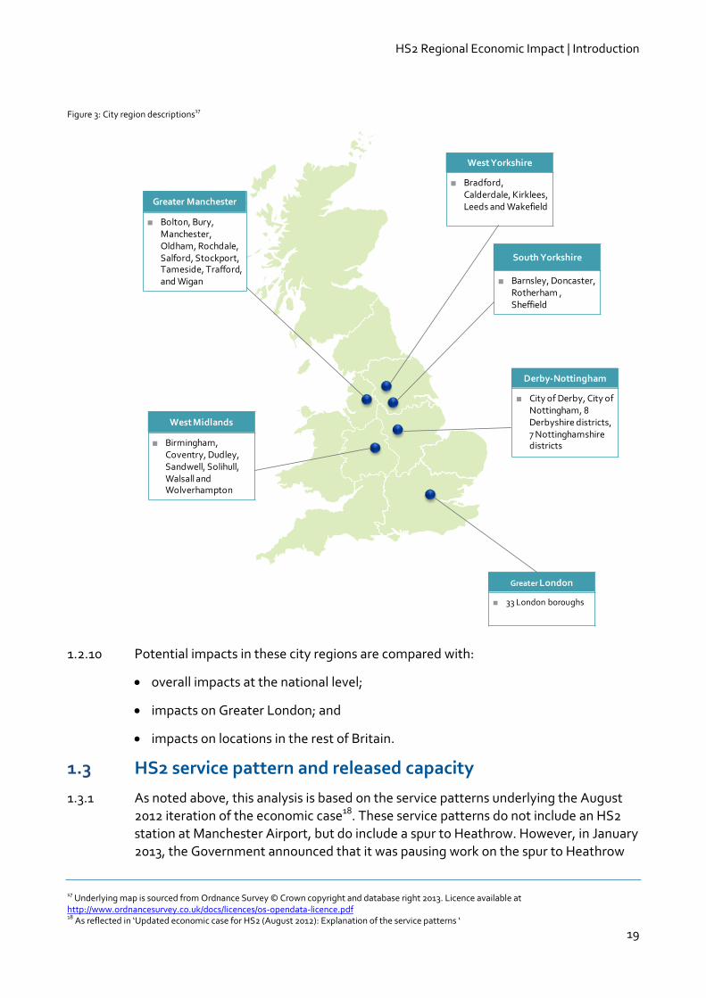
1.2.9 The city regions considered for this work are those that will have an HS2 station. The city region, rather than simply the city itself, has been selected to better reflect the economic footprint of the areas affected by HS2. The broad location of these city regions (and a description of their respective authorities) is shown in Figure 3 below.
16 We are grateful to the Advisory panel for their input to the project but note that the views expressed in this document are entirely those of the authors
HS2 Regional Economic Impact | Introduction
19
Figure 3: City region descriptions17
1.2.10 Potential impacts in these city regions are compared with:
overall impacts at the national level;
impacts on Greater London; and
impacts on locations in the rest of Britain.
1.3 HS2 service pattern and released capacity
1.3.1 As noted above, this analysis is based on the service patterns underlying the August 2012 iteration of the economic case18. These service patterns do not include an HS2 station at Manchester Airport, but do include a spur to Heathrow. However, in January 2013, the Government announced that it was pausing work on the spur to Heathrow
17 Underlying map is sourced from Ordnance Survey © Crown copyright and database right 2013. Licence available at http://www.ordnancesurvey.co.uk/docs/licences/os-opendata-licence.pdf 18 As reflected in ‘Updated economic case for HS2 (August 2012): Explanation of the service patterns ‘
West Yorkshire
■ Bradford, Calderdale, Kirklees, Leeds and Wakefield
South Yorkshire
■ Barnsley, Doncaster, Rotherham , Sheffield
Derby-Nottingham
■ City of Derby, City of Nottingham, 8 Derbyshire districts, 7 Nottinghamshire districts
Greater Manchester
■ Bolton, Bury, Manchester, Oldham, Rochdale, Salford, Stockport, Tameside, Trafford, and Wigan
West Midlands
■ Birmingham, Coventry, Dudley, Sandwell, Solihull, Walsall and Wolverhampton
Greater London
■ 33 London boroughs

HS2 Regional Economic Impact | Introduction
20
pending the outcome of the work of the Airports Commission chaired by Sir Howard
Davies, and the initial preferred route for Phase Two that is currently out to consultation does include a Manchester Airport High Speed Station. Therefore, as noted in Section 3.2, there is scope to update the analysis contained in this report as subsequent iterations of the economic case become available.
1.3.2 The HS2 service pattern includes 18 trains per hour (tph) in each direction on the southern route into and out of London Euston, of which half are wholly contained on HS2 infrastructure and half run on to the classic network19.
1.3.3 The project also includes a major re-design of a significant proportion of the classic rail network, using the additional capacity provided by HS2 to enhance frequency, connectivity and capacity elsewhere, as summarised at the end of Section 6.3 in the technical appendix.
1.3.4 Investment in HS2 will change the way in which businesses can access other businesses, as well as their potential employees. The analytical framework developed for this analysis draws on measures of connectivity that capture an area’s connections
to businesses and to labour markets by rail. These measures are often referred to as ‘effective market sizes’. For a given area, its connectivity (or effective market size) will be governed by:
the time, cost and ease of rail travel to other areas;
the number of businesses and potential employees in those other areas; and
the willingness of those businesses and potential employees to accept the given time, cost and ease of rail travel.
1.3.5 Therefore, areas with faster rail services, higher frequencies and/or fewer interchanges (and therefore ‘easier’ journeys), more destination options, and/or connections to denser areas of economic activity would have larger business-to-business and labour market sizes. Investment in HS2 will therefore have a significant impact on the effective market sizes of different areas. Further details of how measures of connectivity (or effective market size) are derived are set out in Section 4.2 of the report.
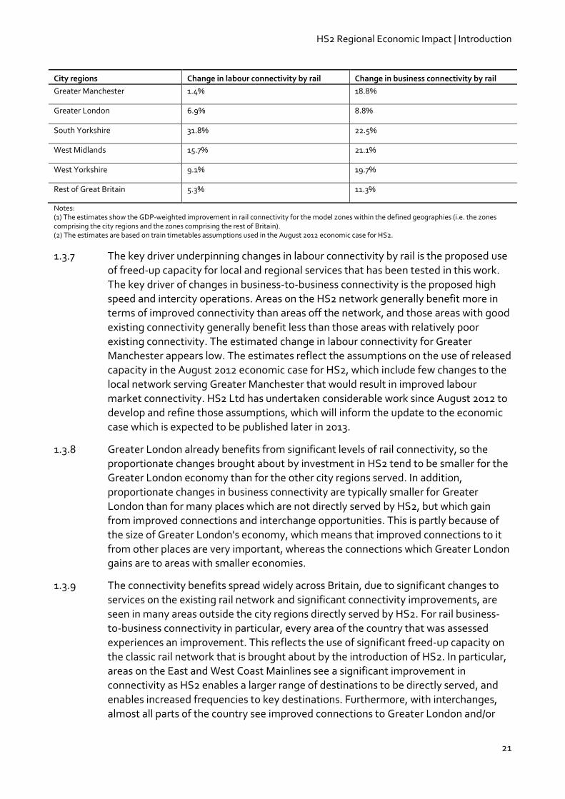
1.3.6 Table 3 shows estimates of changes in business-to-business and labour market
connectivity generated by the package of high-speed and classic rail service
improvements modelled in the August 2012 economic case for the key economic
centres in each city region.
Table 3: Average change in connectivity by city region in 2037 after investment in HS2
City regions Change in labour connectivity by rail Change in business connectivity by rail
Derby-Nottingham 14.7% 23.2%
19 The service pattern that has been assessed includes services to Heathrow (as per the August 2012 Economic Case), which does not now form part of phase two of the HS2 network (set out in the January 2013 Command Paper). The removal of these services would reduce the number of train paths on the London Birmingham section down to 16tph
HS2 Regional Economic Impact | Introduction
21
City regions Change in labour connectivity by rail Change in business connectivity by rail
Greater Manchester 1.4% 18.8%
Greater London 6.9% 8.8%
South Yorkshire 31.8% 22.5%
West Midlands 15.7% 21.1%
West Yorkshire 9.1% 19.7%
Rest of Great Britain 5.3% 11.3%
Notes: (1) The estimates show the GDP-weighted improvement in rail connectivity for the model zones within the defined geographies (i.e. the zones comprising the city regions and the zones comprising the rest of Britain). (2) The estimates are based on train timetables assumptions used in the August 2012 economic case for HS2.
1.3.7 The key driver underpinning changes in labour connectivity by rail is the proposed use
of freed-up capacity for local and regional services that has been tested in this work. The key driver of changes in business-to-business connectivity is the proposed high speed and intercity operations. Areas on the HS2 network generally benefit more in terms of improved connectivity than areas off the network, and those areas with good existing connectivity generally benefit less than those areas with relatively poor existing connectivity. The estimated change in labour connectivity for Greater Manchester appears low. The estimates reflect the assumptions on the use of released capacity in the August 2012 economic case for HS2, which include few changes to the local network serving Greater Manchester that would result in improved labour market connectivity. HS2 Ltd has undertaken considerable work since August 2012 to develop and refine those assumptions, which will inform the update to the economic case which is expected to be published later in 2013.
1.3.8 Greater London already benefits from significant levels of rail connectivity, so the proportionate changes brought about by investment in HS2 tend to be smaller for the Greater London economy than for the other city regions served. In addition,
proportionate changes in business connectivity are typically smaller for Greater London than for many places which are not directly served by HS2, but which gain from improved connections and interchange opportunities. This is partly because of the size of Greater London's economy, which means that improved connections to it from other places are very important, whereas the connections which Greater London gains are to areas with smaller economies.
1.3.9 The connectivity benefits spread widely across Britain, due to significant changes to services on the existing rail network and significant connectivity improvements, are seen in many areas outside the city regions directly served by HS2. For rail business-
to-business connectivity in particular, every area of the country that was assessed experiences an improvement. This reflects the use of significant freed-up capacity on the classic rail network that is brought about by the introduction of HS2. In particular, areas on the East and West Coast Mainlines see a significant improvement in connectivity as HS2 enables a larger range of destinations to be directly served, and enables increased frequencies to key destinations. Furthermore, with interchanges, almost all parts of the country see improved connections to Greater London and/or
HS2 Regional Economic Impact | Introduction
22
other HS2 city regions. Figure 4 below shows the scale of rail business-to-business connectivity changes across Britain in 2037.
Figure 4: Estimated changes in rail business-to-business connectivity in 2037 after investment in HS220
1.4 Structure of this report
1.4.1 In Section 2 we describe the ways in which investment in HS2 has the potential to generate changes in connectivity, which in turn has the potential to improve productivity and influence business location.
1.4.2 In Section 3 we provide a brief commentary on the available methodological approaches and assumptions for assessing the impacts of connectivity on the economy, followed by a description of how the approach might be developed further and refined.
1.4.3 In Section 4 we describe the methodology used to estimate the potential ranges of
economic impacts in this report. In Section 5 we describe the initial set of outputs of this analysis and how they might be interpreted.
1.4.4 Finally, we provide technical appendices that provide more detailed descriptions of the analysis undertaken.
20 Underlying map is sourced from Ordnance Survey © Crown copyright and database right 2013. Licence available at http://www.ordnancesurvey.co.uk/docs/licences/os-opendata-licence.pdf
HS2 Regional Economic Impact | HS2 and the city region economies
23
2 HS2 and the city region economies 2.1 Potential impacts
2.1.1 There are a number of ways in which investment in HS2 has the potential to affect medium- to long-run economic outcomes. In this section, we describe some of the important economic linkages that it would be helpful to capture in analysing the economic impacts of HS2. However, it has not been possible to capture all of these due to data constraints and the complexity of the analysis that would be required. Sections 3 and 4 describe appropriate methodologies which are available and the methodology that we have employed, including a discussion of those impacts that it has been possible to represent and those that could not be represented.
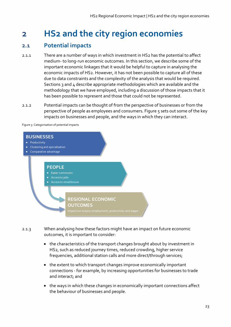
2.1.2 Potential impacts can be thought of from the perspective of businesses or from the
perspective of people as employees and consumers. Figure 5 sets out some of the key impacts on businesses and people, and the ways in which they can interact.
Figure 5: Categorisation of potential impacts
2.1.3 When analysing how these factors might have an impact on future economic outcomes, it is important to consider:
the characteristics of the transport changes brought about by investment in HS2, such as reduced journey times, reduced crowding, higher service frequencies, additional station calls and more direct/through services;
the extent to which transport changes improve economically important connections - for example, by increasing opportunities for businesses to trade and interact; and
the ways in which these changes in economically important connections affect the behaviour of businesses and people.
REGIONAL ECONOMIC OUTCOMESImpacts on output, employment, productivity and wages
BUSINESSES● Productivity
● Clustering and specialisation
● Comparative advantage
PEOPLE● Easier commutes
● Access to jobs
● Access to retail/leisure

HS2 Regional Economic Impact | HS2 and the city region economies
24
Business impacts: productivity
2.1.4 Reduced transport costs following infrastructure investments will:
enable businesses to connect more easily with potential suppliers, enabling them to access higher-quality and/or lower-cost inputs;
enable businesses to connect more easily with potential customers, enabling them to supply markets further afield; and
improve the functioning of the labour market, increasing the effective size of
the market and allowing skills to be better matched to employment opportunities.
2.1.5 These effects are illustrated in Figure 6.
Figure 6: Why the connectivity of a business location matters
2.1.6 Together, these changes in connectivity can enable economies of scale within firms and within sectors and cities that boost productivity.
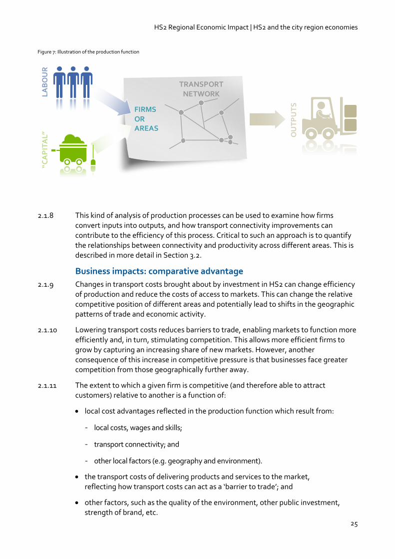
2.1.7 Put simply, firms take labour (i.e. workers) and capital (i.e. data, intellectual property, branding, land, raw materials, etc.) and use their production technology, the transport network and other environmental factors to produce outputs (Figure 7).
● How difficult is the journey?
● How far is too far?
LABOUR MARKETWhat skills do they have?
How many of them are there?
INTERMEDIATE GOODSMARKET/B2B:Who are they?
How many of them are there?
CONSUMER MARKETS/B2C:How large is the market?
WHO CAN I TRADE WITH?
● How difficult is the trip?
● How far is too far?
● How difficult is the commute?
● How far is too far?
HS2 Regional Economic Impact | HS2 and the city region economies
25
Figure 7: Illustration of the production function
2.1.8 This kind of analysis of production processes can be used to examine how firms
convert inputs into outputs, and how transport connectivity improvements can contribute to the efficiency of this process. Critical to such an approach is to quantify the relationships between connectivity and productivity across different areas. This is described in more detail in Section 3.2.
Business impacts: comparative advantage
2.1.9 Changes in transport costs brought about by investment in HS2 can change efficiency of production and reduce the costs of access to markets. This can change the relative competitive position of different areas and potentially lead to shifts in the geographic patterns of trade and economic activity.
2.1.10 Lowering transport costs reduces barriers to trade, enabling markets to function more efficiently and, in turn, stimulating competition. This allows more efficient firms to grow by capturing an increasing share of new markets. However, another consequence of this increase in competitive pressure is that businesses face greater competition from those geographically further away.
2.1.11 The extent to which a given firm is competitive (and therefore able to attract customers) relative to another is a function of:
local cost advantages reflected in the production function which result from:
local costs, wages and skills;
transport connectivity; and
other local factors (e.g. geography and environment).
the transport costs of delivering products and services to the market, reflecting how transport costs can act as a ‘barrier to trade’; and
other factors, such as the quality of the environment, other public investment, strength of brand, etc.
LA
BO
UR
“CA
PIT
AL” O
UT
PU
TS
TRANSPORT NETWORK
FIRMS OR AREAS

HS2 Regional Economic Impact | HS2 and the city region economies
26
2.1.12 In different sectors and markets, the relative importance of production costs and transport distribution costs will vary.
2.1.13 Transport costs for accessing markets include both business travel (for meeting customers and delivering labour-intensive services) and freight (for distributing outputs/products). In the markets that are most likely to be affected by investment in HS2, such as professional services, transport costs for accessing markets are typically the costs, time and inconvenience of making business trips.
2.1.14 By way of illustration, a business services company located in central Manchester might be able to grow its share of the business services market in Birmingham as a result of in-vehicle rail journey times being reduced from 88 to 41 minutes21. Similarly the same firm might also be able to provide services to clients in London - where previously the 128-minute in-vehicle rail journey was prohibitive it now, offers the
potential for gains in market share, having been reduced to 68 minutes. In general, firms will face greater competition from businesses located in other areas - for example, firms located in Manchester will have to compete more strongly for the Manchester market with firms located in Birmingham. It will be important to capture what is often called the ‘two-way road effect', where an improvement in transport can be seen as both a competitive opportunity and a competitive threat, with the potential for the stronger market to 'win' at the expense of weaker markets.
2.1.15 Over time, as a result of many factors, including connectivity changes, business location decisions can change. This could result in changes to the distribution of economic activity. A recent study22 of the location decisions of 30,000 US business headquarters, around 5% of which relocate every year, found that headquarters have become increasingly concentrated in medium-sized service-oriented metropolitan
areas. The areas that have received most inwards moves (and moves which have not then been reversed) are those with a high level of business activity, relatively low wages and, above all, good business transport links (which in the United States, typically means good links to airports).
Impacts on people
2.1.16 Reduced transport costs could affect people in three main ways:
by making commuting easier - some people may decide to go to work or stay in work rather than retiring early, studying or staying at home;
by improving the range of jobs that are accessible - people may be able to access jobs that provide a better match for their skills; and
by improving access to leisure and retail opportunities - people may be able to access a wider range of products or reach similar products at cheaper prices.
2.1.17 However, competitive labour market forces are also increased, so people can also face greater competition for jobs.
21 http://www.hs2.org.uk/phase-two/facts-figures. 22 Strauss-Kahn, V. and Vives, X, (2009). "Why and where do headquarters move?", Regional Science and Urban Economics, Elsevier, vol. 39(2), pages 168-186, March.
HS2 Regional Economic Impact | Methodological approaches
27
2.1.18 These impacts on people, and the related incentives they promote, have the potential
to result in changes over time in the residential location of the population, and consequently of the labour supply. These impacts will also depend in part on other local infrastructure and resources (e.g., schools, health facilities, etc.).
Interaction between business and labour impacts
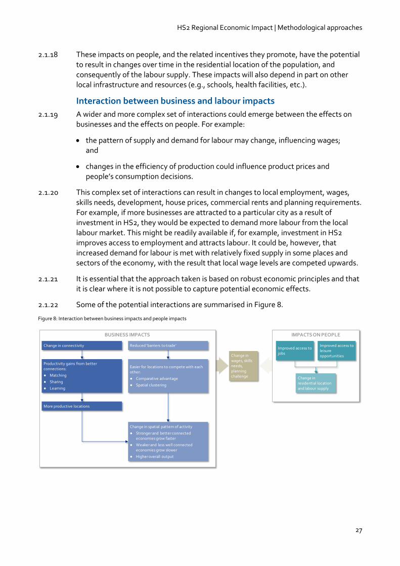
2.1.19 A wider and more complex set of interactions could emerge between the effects on businesses and the effects on people. For example:
the pattern of supply and demand for labour may change, influencing wages; and
changes in the efficiency of production could influence product prices and people’s consumption decisions.
2.1.20 This complex set of interactions can result in changes to local employment, wages, skills needs, development, house prices, commercial rents and planning requirements. For example, if more businesses are attracted to a particular city as a result of investment in HS2, they would be expected to demand more labour from the local labour market. This might be readily available if, for example, investment in HS2 improves access to employment and attracts labour. It could be, however, that increased demand for labour is met with relatively fixed supply in some places and sectors of the economy, with the result that local wage levels are competed upwards.
2.1.21 It is essential that the approach taken is based on robust economic principles and that it is clear where it is not possible to capture potential economic effects.
2.1.22 Some of the potential interactions are summarised in Figure 8.
Figure 8: Interaction between business impacts and people impacts
Change in wages, skills needs, planning challenge
BUSINESS IMPACTS
Productivity gains from better connections:
● Matching
● Sharing
● Learning
Easier for locations to compete with each other:
● Comparative advantage
● Spatial clustering
More productive locations
Change in connectivity Reduced ‘barriers to trade’
Change in spatial pattern of activity
● Stronger and better connected economies grow faster
● Weaker and less well connected economies grow slower
● Higher overall output
IMPACTS ON PEOPLE
Improved access to jobs
Improved access to leisure opportunities
Change in residential location and labour supply
HS2 Regional Economic Impact | Methodological approaches
28
3 Methodological approaches 3.1 Background to development
3.1.1 The key objective of this work has been to develop an analytical framework that appropriately captures the impact of transport connectivity on the economy and is grounded in robust economic theory. This, in turn, allows the scale and distribution of economic impacts arising from investment in HS2 to be better understood. However, there is no ‘off the shelf’ methodology that is widely used in UK transport appraisal to assess the complex issues of productivity, trade and regional economic competitiveness that are raised by investment in HS2. Any approach will therefore have strengths and weaknesses. This highlights the importance of recognising constraints and uncertainties and developing a flexible approach that can be improved over time.
3.1.2 Conventional transport appraisal guidance from the Department for Transport (DfT) is primarily focused on the welfare benefits to transport users, such as the value of time savings and other associated impacts on safety and the environment. Guidance is also provided for capturing some of the impacts of transport on the economy (in terms of GDP), but this is limited to the assumption of fixed land use and business behaviour. It therefore does not provide a guide to how investment in HS2 could change the competitive forces that influence the structure, size and geographic pattern of economic activity in Britain.
3.1.3 The economic benefits appraised for the HS2 economic case are governed by conventional appraisal guidance. This has allowed the monetised costs and benefits of the scheme to be assessed on a comparable basis, in line with Treasury’s Green Book appraisal approach and DfT’s Transport Analysis Guidance23.
3.1.4 This new study has sought to take a different approach to conventional appraisal
techniques in order to understand how investment in HS2 will have an effect on productivity and inter-regional competition and hence medium- to long-term economic growth. This is in line with the potential impacts identified in Section 2, focusing on the impacts on businesses.
3.1.5 To develop such an approach, we have built on analytical approaches that have been used in similar contexts. This has been based on a review of the existing literature, KPMG’s own experience, and consultation with the HS2 Ltd advisory panel.
3.1.6 In this section, we summarise alternative approaches and discuss some of their strengths and weaknesses.
23 The Treasury’s Green Book sets the overarching framework for how projects are assessed across different Government departments, in order to provide a consistent basis for project appraisal and evaluation of value for money to the taxpayer. DfT’s web-based Transport Analysis Guidance (webTAG) provides guidance on the conduct of appraisals of major highway and public transport schemes, and is a requirement for all proposed transport projects that require Government approval.
HS2 Regional Economic Impact | Methodological approaches
29
3.2 Analytical approaches
Available approaches
3.2.1 In reviewing the analytical approaches potentially available to this work, we have focused on those which specifically address the relationship between the connectivity provided by the transport network and its impacts on productivity and business location. Therefore, the remainder of this section does not consider methodologies to assess local regeneration impacts (e.g. site-specific development around HS2 stations) or the short-term impacts of expenditure on the construction and operation of HS2 and the associated positive multiplier effects, or conventional welfare-based appraisal techniques.
3.2.2 There are a range of approaches that could be taken to examining and attempting to quantify the economic consequences of investment in HS2 on the areas that it will
serve and the British economy as a whole. Approaches range from qualitative approaches and survey-based techniques to quantitative modelling approaches.
3.2.3 To ensure that a consistent approach is applied in each area, we have rejected options which rely on information that is only available for some areas. For example, in some areas transport and land use interaction models exist already, but these are inconsistent and are not available for all areas to be served by HS2. Indeed, the implications of significant change to the classic rail network touch on many areas of the country, so any approach must deal consistently with all areas.
3.2.4 We also rejected qualitative approaches in favour of a consistent analytical framework which will return quantified results based on a given set of input assumptions, recognising the uncertainties that these assumptions introduce. This argues for a national model of transport connectivity and its economic outcomes.
3.2.5 Other approaches which have been employed separately capture aspects of:
transport’s impact on productivity through the agglomeration of business activity - for example, by Dan Graham and his team at Imperial College London24;
the specific impacts of rail connectivity on agglomeration and productivity - for
example, in previous work by KPMG and the Spatial Economics Research Centre at the London School of Economics on the impacts of investment in the Northern Rail Hub;
links between connectivity and business location - for example, in work undertaken by the city regions to support the economic prioritisation of their local infrastructure investment programmes; and
the feedback effects between households, businesses, developers and the transport sector - for example, in Land Use and Transport Interaction (LUTI) modelling, which is becoming increasingly common within transport
24 Graham, D.J. et al (2009), "Transport investment and the distance decay of agglomeration benefits", Centre for Transport Studies, Imperial College London, London.

HS2 Regional Economic Impact | Methodological approaches
30
appraisal25.
3.2.6 However, existing applications do not bring these together in a way that addresses the specific strategic questions about the potential impact of investment in HS2 on the shape of the national economy and on the areas that HS2 serves.
3.2.7 A key trade-off occurs in the level of geographical detail which different approaches can support. Some approaches rely on relatively simple socio-economic data, such as population and workplace jobs, which is available for small local areas. Others have more extensive data demands and require information on economic output labour productivity or capital inputs, which may not exist at smaller geographical scales.
3.2.8 This work has made use of data from the transport model, PLANET Long Distance (PLD), which separates Britain into 235 zones (each representing one or more local authority districts26). A map of these zones is provided in Section 6.2 of the technical
appendices. This approach was deemed to strike the right balance between effectively capturing the geographical impacts of investment in HS2 and working with appropriate and available data. It is also consistent with the transport models that have been developed to appraise HS2 and from which we are able to draw input data.
3.2.9 Given these decisions and constraints, we have considered three broad methodological approaches which are set out in Figure 9 below. The subsequent section then sets out the key advantages and disadvantages of each of these approaches, and the extent to which they have been tried and tested to assess the impacts of potential transport investment.
25 In conventional DfT appraisal, the application of a LUTI model does not form part of the central case analysis. However, under DfT's webTAG Unit 3.5.14: The Wider Impacts Sub-Objective, the impact of transport on employment and residential location can be addressed through sensitivity analysis using a LUTI model. 26 The PLANET Modelling Framework is a suite of transport models used by HS2 Ltd to represent the time, cost and demand of travel between origin and destinations (represented as model zones) across Great Britain using different service pattern scenarios. The PLANET Long Distance model forms part of this modelling framework. Further information is available through HS2 Ltd’s website.

HS2 Regional Economic Impact | Methodological approaches
31
Figure 9: Alternative analytical approaches
Advantages and disadvantages
3.2.10 Approaches based on simple connectivity relationships are long established and directly analyse the relationships between connectivity and economic outcomes
based on historic cross-sectional data. For example, models have been developed which examine the statistical relationship between transport connectivity (as defined in this study) and the density of employment (e.g. workplace jobs per km2) in different areas. However, these approaches say little about how or why these relationships work and are the least sophisticated of the three approaches. The simplicity of the approach typically means that:
This approach can be based on simpler datasets, which reduces the need to
make assumptions or develop proxies in order to build the modelling approach, and it provides for a more transparent assessment of the impacts of transport on the economy.
However, this approach can lack the flexibility to capture more nuanced relationships and does not take account of the potentially complex trade
interactions between different locations, which mean that, for a given region, transport improvements can be both an opportunity (through access to larger markets) and a threat (through exposure to more efficient competitors).
3.2.11 The productivity and business location approach is more complex and tells us much more about the intermediate transmission mechanisms, (with a more refined approach to capturing how transport changes affect business productivity, location decisions, access to markets, etc.), and established analytical approaches are again
SIMPLE COMPLEX
Simple connectivity approach
Connectivity directly drives outcome variables (GVA, GDP, employment, wages, etc)
1
ALTERNATIVE APPROACH
Productivity and business location approach
a) Production function estimationBased on micro-economic foundations and accounting for labour cost and quality differences to capture impacts of rail changes
b) Business locationLocal cost advantages from agglomeration (a concentrating force) and transport costs (a dispersing force) drive trade between locations and business relocation effects
2
PREFERRED APPROACH
General equilibrium approach
Capturing supply and demand behaviour in product, labour and capital markets and the full interactions between them
3
POSSIBLE LONGER TERM APPROACH
HS2 Regional Economic Impact | Methodological approaches
32
available. These approaches have the potential to address a broader range of the potential impacts associated with investment in HS2, including how:
productivity in the city regions and surrounding areas might be affected
(taking account of the scale, quality and cost of inputs in the production of firms’ output by sector and geographic location); and
trade relationships, both between different city regions and between a given city region and its surrounding area, might be affected.
3.2.12 The impacts of transport connectivity on productivity are well established through many academic studies, although some changes are required to capture the specific role of rail connectivity. Models of trade relationships are also common and are based on the distance or transport costs between locations. Together, the combination of productivity analysis and business location analysis provides a coherent structure and
a good representation of the impacts of investment in HS2 on businesses. It can be implemented with existing data and constraints while offering the potential for future refinement and development where uncertainties remain.
3.2.13 General equilibrium27 approaches have the potential to capture the impacts of investment in HS2 with yet more sophistication, including the full range of interactions and relationships between product, capital and labour markets (with the last of these explicitly capturing the impact on wages and labour supply). There is, however, a lack of consensus on how to deploy these types of methodology within the context of transport appraisal, and much uncertainty associated with their analytical complexity. Given this complexity and the fact that it is not a tried and tested approach, the development of a general equilibrium model has not been deemed to be practical for the purposes of this work. However, the development of this type of analysis could be a potential longer-term aspiration.
Preferred approach
3.2.14 An analytical approach based on the productivity and business location methodology is considered most appropriate for the purposes of this work. This analytical approach focuses on the estimation of gains in productivity arising from improved business and labour market connectivity, followed by an assessment of the potential redistribution of these gains as firms compete with each other. Further details of this approach are described in the next section.
27 Dixon, P and Jorgenson, D (2013) "Handbook of Computable General Equilibrium Modelling", Elsevier.
HS2 Regional Economic Impact | Methodology to estimate the economic impacts of investment in HS2
33
4 Methodology to estimate the economic impacts of investment in HS2 In this section we describe the methodology (and data) used to derive initial estimates of the potential regional economic impacts of investment in HS2. More detailed technical descriptions of the methodology and data are then provided in Section 6, in the technical appendices.
4.1 Building an approach
4.1.1 As described in Section 2, investment in HS2 has the potential to result in a number of impacts on business productivity and competitiveness, with associated impacts on the labour market.
4.1.2 These effects interact over time and have the potential to result in changes in output and the spatial distribution of economic activity.
4.1.3 The impacts are clearly uncertain, and they depend on macro- and micro-level interactions between firms, within firms and with the labour market. Moreover, they depend on assumptions about how the economy and transport patterns will develop in future. We have used standard assumptions for these future ‘Do Minimum’ trends which are based on information from DfT and HS2 Ltd, and which are consistent with assumptions that have been made in the transport modelling for the scheme28.
4.1.4 The approach used to derive the initial results set out in Section 5 has been designed to capture to potential range of impacts presented in Section 2.1. There is, however, still a wider scope for further development of the approach and analysis, as set out in Section 4.6.
Productivity changes
4.1.5 Productivity changes are driven by changes in connectivity (among other things), including reduced generalised costs29 between businesses, and between businesses and labour, which enable specialisation and agglomeration. Academic literature has identified some important ways in which these impacts can arise, including:
specialisation of labour and within supply chains;
matching of skills to jobs and, suppliers to customers;
sharing of inputs with a minimum efficient scale; and
learning through knowledge spill-overs from denser economic agglomerations30.
28 ‘Do Minimum’ refers to a situation without HS2 or the associated re-deployed capacity. In other words it is the ‘reference’ case against which impacts are assessed 29 'Generalised cost' is an estimate of the monetary and non-monetary costs of a making a journey. It includes out-of-pocket expenses and a cash-equivalent value of travel time based on passengers’ value of time. Further details of the construction of generalised cost and the specification of the decay curves are reported in the Technical Appendices. 30 Duranton, G. and Puga, D. (2003) Micro-foundations for Urban Agglomeration Economies, NBER Working Paper No. 9931

HS2 Regional Economic Impact | Methodology to estimate the economic impacts of investment in HS2
34
4.1.6 In practice, it is very difficult to disentangle the different factors that lie behind
agglomeration economies, but all of these economies share a common feature of high levels of connectivity. To address this, we have derived a production function which describes how efficiently areas can combine labour with other inputs and how differences in connectivity affect efficiency and thus total output for a given level of input. The production function is calibrated on 2010 base year data and estimated on cross-sectional data from the 235 model zones.
Business location impacts
4.1.7 Stronger economies with lower production costs could out-compete weaker ones with higher production costs when the barriers to trade are reduced. At the same time, the transport system is one of the driving forces that generate the local production cost advantages. We have developed a model which explicitly captures competition and trade interactions between local economies and the ways in which they are affected
by changes in the transport system. This is the most appropriate and direct way of examining the impacts of investment in HS2 on the distribution of economic activity across the country and on the widely discussed North-South divide.
4.1.8 In the model the allocation of economic output between zones depends on the competitive position of each zone when it is selling in each market. It therefore explicitly captures trade between zones and the transport system's effect upon this. Thus, a local supplier may be competitive because the combination of its production costs and transport costs to market are lower than those of competitors further afield. However, if the costs of transport to that market fall, more efficient companies from further away may out-compete the local supplier.
4.1.9 Investment in HS2 is expected to affect both local production cost advantages and the
costs of trade between zones. The competitiveness of a producing location when selling to a particular market where consumption takes place is therefore a function of:
the local costs of production in the producing zone; and
the costs of supplying the goods or services to the zone in which consumption takes place.
4.1.10 This model of competitiveness and trade is used to examine which areas see a competitive advantage and grow due to investment in HS2, and which suffer as more competitive areas compete away their markets. A full description of the productivity and business location model is provided in Section 6.3 of the technical appendices.
4.1.11 Having analysed the range of potential productivity and competitiveness-related impacts, it becomes possible to identify the types of growth that might be expected in particular locations and the potential planning, skills and other steps the city regions may need to take in order to prepare for HS2.
4.1.12 All of these approaches rely on suitable information about the transport network and the connectivity that it provides. Sections 4.2 to 4.4 below explain in more detail:
what is meant by 'connectivity' and how it has been measured;
HS2 Regional Economic Impact | Methodology to estimate the economic impacts of investment in HS2
35
the modelling of productivity impacts and the production function; and
the modelling of business location effects between local areas.
4.2 Measuring connectivity
4.2.1 Measurements of connectivity have three key elements:
information reflecting the difficulty of travel, which we capture using generalised costs of travel;
a ‘deterrence function’ or ‘decay curve’, describing how the opportunity to trade or interact reduces as the generalised cost of travel increases; and
information about what is being accessed or connected to (e.g. potential employees or other businesses).
4.2.2 In this section, we briefly describe our approach to these issues, including key assumptions, such as dividing Britain into a number of model zones and grouping similar kinds of economic activity into sectors on which we undertake our analysis.
Data and segmentation
4.2.3 The geographic scope of our analysis is determined by the data available and is based on HS2 Ltd’s existing zonal structure (as reflected in the PLD Model), which divides England, Scotland and Wales into 235 zones that are broadly consistent with local authority districts. However, there are some important exceptions. For example, the four districts of Greater Manchester in which the Metrolink light rail network operated prior to 2012 (i.e. Bury, Manchester, Salford and Trafford) are aggregated into one zone. Greater London is represented by eight zones. A map of PLD zones is provided
in Section 6.2 of the technical appendices. Transport journey data, socio-economic data and measures of connectivity are all based on this geographical unit.
4.2.4 Transport users have been segmented into:
rail commuters;
car commuters;
rail business travellers; and
car business travellers.
4.2.5 As each of the underlying 235 PLD zones is relatively large, the analysis necessarily assumes no economic benefits from trips within the same zone. The changes
associated with investment in HS2 will tend to operate over longer distances, so this is not considered a significant weakness in the analysis of business-to-business impacts, but may lead to an under-estimation of labour market impacts.
4.2.6 Moreover, the underlying PLD modelling captures only the impacts on passenger journeys. Thus, it does not capture potential incremental economic benefits associated with rail freight. This is potentially a more significant omission because changes to the rail network associated with investment in HS2 will affect the number
HS2 Regional Economic Impact | Methodology to estimate the economic impacts of investment in HS2
36
of network paths available for rail freight, which may be of significant benefit for some
types of economic activity. Our findings show effects which are predominantly in the business services and consumer services markets, which do not rely strongly on rail freight.
4.2.7 In this analysis, the relevant sectors of the economy are assumed to be represented by four sectors, consistent with the DfT’s Transport Analysis Guidance31:
construction;
consumer services (which includes hospitality, land, retail, transport and wholesale services);
manufacturing; and
producer services (which includes financial, insurance, IT and other business services).
4.2.8 These cover around two-thirds of the economy and exclude sectors such as agriculture, which are considered highly unlikely to benefit from investment in HS2.
4.2.9 While it is theoretically possible to refine the analysis to incorporate a more disaggregated view of the relevant economic sectors, to date a lack of consistent, independent data at the appropriate levels of geography has prevented such an approach.
Generalised costs
4.2.10 The transport cost impacts of investment in HS2 are appraised with reference to ‘generalised costs’, which represent the time, financial cost and other journey factors
(crowding, waiting time, interchange time, etc) in pence-equivalent costs between each pair of zones. Time-based factors are converted to pence using evidence of how people value different aspects of the journey experience. These parameters are
derived from the DfT’s guidance and are consistent with the assumptions made within HS2 Ltd’s transport modelling. Time spent waiting and interchanging is given a higher weighting than in-vehicle time, reflecting the inconvenience people associate with these journey components based on their observed travel behaviour.
4.2.11 Generalised costs have been sourced from the PLD model for car and rail trips. These differ between people travelling for different journey purposes because different segments of the market have different behavioural responses to, for example, waiting for services or the inconvenience of interchanging. Journey costs change both as a result of the direct impacts of investment in HS2, and due to indirect factors such as reduced congestion and motoring costs. Direct impacts include:
in-vehicle journey time reductions as a result of faster services;
journey time reductions as a result of the availability of more direct services;
frequency improvements (e.g. on the classic network);
31 DfT’s web-based Transport Analysis Guidance (webTAG) provides guidance on the conduct of transport appraisal, including recommended data sources, to provide a consistent basis upon which potential transport investment is assessed.
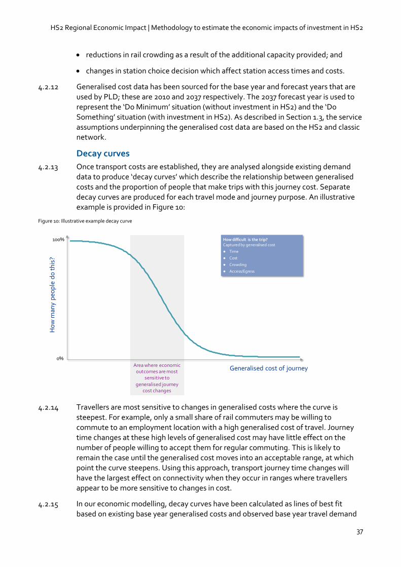
HS2 Regional Economic Impact | Methodology to estimate the economic impacts of investment in HS2
37
reductions in rail crowding as a result of the additional capacity provided; and
changes in station choice decision which affect station access times and costs.
4.2.12 Generalised cost data has been sourced for the base year and forecast years that are used by PLD; these are 2010 and 2037 respectively. The 2037 forecast year is used to represent the ‘Do Minimum’ situation (without investment in HS2) and the ‘Do Something’ situation (with investment in HS2). As described in Section 1.3, the service assumptions underpinning the generalised cost data are based on the HS2 and classic network.
Decay curves
4.2.13 Once transport costs are established, they are analysed alongside existing demand data to produce ‘decay curves’ which describe the relationship between generalised costs and the proportion of people that make trips with this journey cost. Separate
decay curves are produced for each travel mode and journey purpose. An illustrative example is provided in Figure 10:
Figure 10: Illustrative example decay curve
4.2.14 Travellers are most sensitive to changes in generalised costs where the curve is steepest. For example, only a small share of rail commuters may be willing to commute to an employment location with a high generalised cost of travel. Journey time changes at these high levels of generalised cost may have little effect on the
number of people willing to accept them for regular commuting. This is likely to remain the case until the generalised cost moves into an acceptable range, at which point the curve steepens. Using this approach, transport journey time changes will have the largest effect on connectivity when they occur in ranges where travellers appear to be more sensitive to changes in cost.
4.2.15 In our economic modelling, decay curves have been calculated as lines of best fit based on existing base year generalised costs and observed base year travel demand
Area where economic outcomes are most
sensitive to generalised journey
cost changes
Ho
w m
any
peo
ple
do
th
is?
Generalised cost of journey
100%
0%
How difficult is the trip?Captured by generalised cost
● Time
● Cost
● Crowding
● Access/Egress
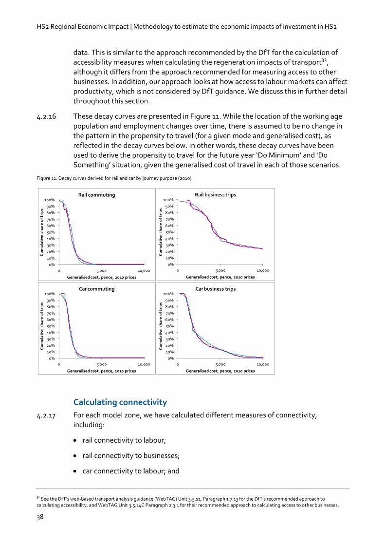
HS2 Regional Economic Impact | Methodology to estimate the economic impacts of investment in HS2
38
data. This is similar to the approach recommended by the DfT for the calculation of
accessibility measures when calculating the regeneration impacts of transport32, although it differs from the approach recommended for measuring access to other businesses. In addition, our approach looks at how access to labour markets can affect productivity, which is not considered by DfT guidance. We discuss this in further detail throughout this section.
4.2.16 These decay curves are presented in Figure 11. While the location of the working age population and employment changes over time, there is assumed to be no change in the pattern in the propensity to travel (for a given mode and generalised cost), as reflected in the decay curves below. In other words, these decay curves have been used to derive the propensity to travel for the future year ‘Do Minimum’ and ‘Do Something’ situation, given the generalised cost of travel in each of those scenarios.
Figure 11: Decay curves derived for rail and car by journey purpose (2010)
Calculating connectivity
4.2.17 For each model zone, we have calculated different measures of connectivity, including:
rail connectivity to labour;
rail connectivity to businesses;
car connectivity to labour; and
32 See the DfT’s web-based transport analysis guidance (WebTAG) Unit 3.5.11, Paragraph 1.7.13 for the DfT’s recommended approach to calculating accessibility, and WebTAG Unit 3.5.14C Paragraph 2.3.1 for their recommended approach to calculating access to other businesses.
0%
10%
20%
30%
40%
50%
60%
70%
80%
90%
100%
0 5,000 10,000
Cu
mu
lati
ve s
ha
re o
f tr
ips
Generalised cost, pence, 2010 prices
Rail commuting
0%
10%
20%
30%
40%
50%
60%
70%
80%
90%
100%
0 5,000 10,000
Cu
mu
lati
ve s
ha
re o
f tr
ips
Generalised cost, pence, 2010 prices
Rail business trips
0%
10%
20%
30%
40%
50%
60%
70%
80%
90%
100%
0 5,000 10,000
Cu
mu
lati
ve s
ha
re o
f tr
ips
Generalised cost, pence, 2010 prices
Car commuting
0%
10%
20%
30%
40%
50%
60%
70%
80%
90%
100%
0 5,000 10,000
Cu
mu
lati
ve s
ha
re o
f tr
ips
Generalised cost, pence, 2010 prices
Car business trips
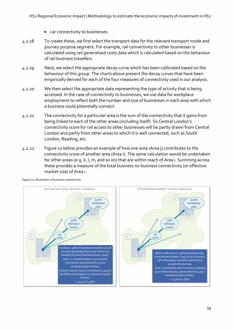
HS2 Regional Economic Impact | Methodology to estimate the economic impacts of investment in HS2
39
car connectivity to businesses.
4.2.18 To create these, we first select the transport data for the relevant transport mode and journey purpose segment. For example, rail connectivity to other businesses is calculated using rail generalised costs data which is calculated based on the behaviour of rail business travellers.
4.2.19 Next, we select the appropriate decay curve which has been calibrated based on the behaviour of this group. The charts above present the decay curves that have been empirically derived for each of the four measures of connectivity used in our analysis.
4.2.20 We then select the appropriate data representing the type of activity that is being accessed. In the case of connectivity to businesses, we use data for workplace employment to reflect both the number and size of businesses in each area with which a business could potentially connect.
4.2.21 The connectivity for a particular area is the sum of the connectivity that it gains from being linked to each of the other areas (including itself). So Central London’s connectivity score for rail access to other businesses will be partly drawn from Central London and partly from other areas to which it is well connected, such as South London, Reading, etc.
4.2.22 Figure 12 below provides an example of how one area (Area j) contributes to the connectivity score of another area (Area i). The same calculation would be undertaken for other areas (e.g. k, l, m, and so on) that are within reach of Area i. Summing across these provides a measure of the total business-to-business connectivity (or effective market size) of Area i.
Figure 12: Illustration of business connectivity
AFTER IMPROVEMENT TO RAIL SERVICESBEFORE ANY RAIL SERVICE CHANGES
i
j
For Area i, 50% of business travellers would accept a generalised journey time of 45 minutes to travel between Areas i and j.
Area i is therefore able to access the businesses represented by 2,500
workplace jobs in Area j
(In other words, Area j contributes 2,500 to the effective business-to-business market
of Area i:
( = 5,000 X 50% )
With a reduction in generalised journey time between Areas i and j to 30 minutes,
75% of business travellers would now accept this journey
Area i is therefore able to access a deeper pool of businesses, represented by 3,750
workplace jobs in Area j
( = 5,000 X 75% )
i
j5,000
workplace jobs
5,000 workplace
jobs
50% willing to
travel
45 mins
75% willing to
travel
30 mins
HS2 Regional Economic Impact | Methodology to estimate the economic impacts of investment in HS2
40
4.2.23 When generalised costs decrease to another area, connectivity increases. The impact of the journey time change will be larger if the journey is sensitive to journey time changes (i.e., on the steep part of the decay curve) and if the other area has an abundance of other businesses with which to connect.
4.2.24 Measures of connectivity are calculated for 2037 using standard data from the DfT on future patterns of workplace employment (for effective business-to-business markets) and working-age residential population (for effective labour markets)33. These use the observed behaviour encapsulated in the decay curves presented above and estimates of future generalised costs in two situations: with and without investment in HS2.
4.2.25 This approach differs from DfT guidance on the calculation of ‘effective density’ in two important respects. First, DfT guidance results in a single measure of connectivity to other businesses, whereas our approach attempts to separately identify the impact of
access to other businesses and access to labour by rail and car. The DfT’s single measure of connectivity is easier to use subsequently in economic analysis, but it makes a number of implicit assumptions. It assumes, for example, that the relative importance of business trips and commuting trips to productivity is equal to the share of trips of each type. Second, the DfT’s approach assumes that the importance of a connection declines exponentially as transport costs increase (a negative exponential decay curve), whereas our approach assumes that the importance of trips declines according to the observed pattern of trip-making.
4.2.26 Both methods have strengths and weaknesses. We have developed our approach to attempt to best represent how the connectivity brought about by investment in HS2 is most likely to affect businesses and regional economic outcomes. As set out in Section 4.6, further work is required to examine the sensitivity of our findings to alternative measures of connectivity.
4.3 Productivity impacts
The production function
4.3.1 The production function for a given business shows the relationship between economic output and inputs to the production process, such as labour and capital.
4.3.2 To analyse how investment in HS2 affects the efficiency, and thus productivity, of different locations in each sector of the economy, we must specify and estimate a production function. Using this production function, we model the economic output in each of the 235 model zones as a function of labour inputs, capital inputs and connectivity to businesses and to labour by rail and car.
4.3.3 When specifying the production function, we hypothesise that different types of transport connectivity can affect the productivity of different areas. We then use statistical analysis to test this hypothesis and examine whether, and to what extent, transport connectivity can help to explain the differences in economic output between places. The findings from this analysis provide us with elasticities, which are then used
33 Data sourced from DfT’s Wider Impacts Dataset provided in WebTAG, Unit 3.5.14: The Wider Impacts Sub-Objective
HS2 Regional Economic Impact | Methodology to estimate the economic impacts of investment in HS2
41
to forecast the impact on productivity of changes in connectivity brought about by investment in HS2.
Data and calibration
4.3.4 The production function methodology described above is based on data for labour inputs and capital inputs used in different model zones and the connectivity measures described in Section 4.2. The technical appendices in Section 6 set out in detail the data used to estimate the production function.
4.3.5 Whilst some information34 is available from studies regarding the productivity impacts of transport changes, significant questions of applicability and transferability prevented their use in this study. In particular, most studies do not attempt to use decay curves based on observed behavioural patterns of travel in their calculation of connectivity; nor do they attempt to separate the different impacts on productivity of
connectivity by mode (i.e. by rail and car) or by market segment (i.e. to business-to-business markets and to labour markets).
4.3.6 In using this approach, average wages by sector in each zone have been estimated by applying regional factors based on the Annual Survey of Hours and Earnings to adjust average pay data in each zone, which has been sourced from DfT’s Wider Impacts Dataset35. For example, North West factors for each sector have been applied to zones in Greater Manchester.
4.3.7 While labour market data is available for each zone, the same cannot be said for information about capital stocks and additions in the production function (e.g. land). This is not generally available on a consistent basis in sufficient detail. It has therefore been necessary to assume that, as local GDP and employment change over time and as a result of investment in HS2, fixed proportions of capital and labour are required in
each sector of the economy in each zone. This is a restrictive assumption which is dictated by data availability.
4.3.8 While there is some empirical support for this assumption36 - which has been used extensively in the economic literature - it does mean that our analysis has been unable to examine whether and how firms may switch between capital and labour inputs in places with different connectivity characteristics. Other studies use financial statements for firms to derive assumptions about capital use. However, in addition to being extremely complex at such a large scale, this approach can be deployed only for smaller firms, where there is a strong match between the physical location of economic activity and the recording of turnover and cost in statutory accounts.
4.3.9 We have tested the sensitivity of our findings to different ways of including or
excluding capital inputs into the production function. We find that including estimates of capital inputs does not have a significant effect on our findings. However, we prefer the generalised approach, which includes estimates of capital inputs because it
34 A good survey of the literature with reference to the UK context is provided in Graham, D.J. (2005) Wider economic benefits of transport improvements: link between agglomeration and productivity, Stage 1 report. Department for Transport, London 35 Department for Transport, WebTAG, Unit 3.5.14: The Wider Impacts Sub-Objective 36 See for example, Douglas, P.H., "The Cobb-Douglas Production Function Once Again: Its History, Its Testing, and Some New Empirical Values". Journal of Political Economy 84 (5): 903–916. October 1976
HS2 Regional Economic Impact | Methodology to estimate the economic impacts of investment in HS2
42
provides a stepping stone towards a more sophisticated treatment of different factor
inputs. In future work, these could include capital inputs as well as, potentially, land and property inputs.
4.3.10 Using this approach to capital and labour inputs and the connectivity measures described in Section 4.2, we have estimated a production function to derive ranges for the potential productivity benefits that are associated with different types of change in transport connectivity. Although there remains some uncertainty about their relative impact, we have examined how productivity impacts are driven by:
connectivity to labour markets by rail;
connectivity to labour markets by car;
connectivity to other businesses by rail; and
connectivity to other businesses by car.
4.3.11 It has not been possible to fully separate the impacts of different types of connectivity on productivity due to correlations between them. This means that areas that tend to be better connected to other businesses also tend to be better connected to labour markets, so it is difficult for statistical approaches to untangle their separate effects. This has limited our ability to distinguish the different effects of, for example, access to businesses in aggregate and access to businesses within the same business sector. It also poses significant challenges for assessing the relative importance of connectivity to markets by car and by rail. Our approach to this is described in more detail in the technical appendices. The elasticities that we have estimated through the production function are shown in Table 4.
Table 4: Estimated elasticities of productivity with respect to connectivity
Construction Consumer services Manufacturing Producer services
Rail connectivity to labour 0.010 0.016 0.007 0.015
Car connectivity to labour 0.010 0.016 0.010 0.017
Rail connectivity to businesses n/a 0.060 0.019 0.073
Car connectivity to businesses 0.025 0.048 0.014 0.056
Note: The elasticity of productivity with respect to connectivity measures the sensitivity of productivity as connectivity changes. An elasticity of 0.010 (1%) means that a doubling of connectivity is expected to result in an increase in productivity of 1%.
4.3.12 By driving productivity improvements, firms are able to produce more units of output for a given amount of inputs, which allows them to compete more effectively for the larger markets that they are now able to serve.
4.3.13 DfT guidance has been developed on methodologies to capture the impact of transport on productivity due to agglomeration. It is not possible to make a direct comparison between our findings and the elasticities contained in DfT guidance or those found in other studies for three reasons:
we have specifically developed parameters which are based on transport generalised costs;
HS2 Regional Economic Impact | Methodology to estimate the economic impacts of investment in HS2
43
we have based our analysis of connectivity on decay curves which have been
derived from observed travel behaviour; and
we have segmented our analysis of connectivity by mode and market segment, i.e. to specifically capture car and rail connectivity to both businesses and to labour markets.
4.3.14 Although direct comparisons are not possible, our findings are in line with the findings of similar studies which report elasticities of productivity with respect to connectivity between 0.01 and 0.20 which corresponds well with our findings. We also find that the producer services sector is the most sensitive to many of the different measures of connectivity (particularly connectivity to other businesses), which again accords well with the findings of similar studies. A stock-take of findings from other studies was prepared for DfT in 2005 which is useful for comparison37.
4.3.15 We have used these findings to estimate the impacts of investment in HS2 on productivity and economic output across Britain in 2037; the results of which are set out in Section 5.
4.3.16 The analysis of productivity assumes that the inputs of labour and capital into the production process are fixed, so that no new additional capital or labour is required for the benefits to be realised.
4.4 Business location impacts
4.4.1 Having forecast the potential range of productivity impacts as a result of the connectivity changes brought about by investment in HS2, we employ a model of trade and business location to examine how this could affect Britain’s economic geography.
4.4.2 The business location model has been developed to reflect the balance between the force of agglomeration economies that tend to concentrate production in denser and more productive locations and the cost of delivering a good or service that tends to disperse activity so that it is produced closer to where it is consumed. Investment in HS2 could affect the balance between these and alter the geographical balance of activity across Britain.
4.4.3 The model we have developed captures these forces through:
the local cost production advantages of different locations which support the concentration of activity in the most productive locations; and
transport costs which support more dispersed activity by protecting more local producers from competition.
4.4.4 The productivity analysis is used to derive measures of production costs in each location. The model of business location is used to allocate UK economic output in the
four different business sectors to different model zones. In this sense it is ‘zero sum’
37 Graham, D.J. (2005) Wider economic benefits of transport improvements: link between agglomeration and productivity, Stage 1 report, Department for Transport, London

HS2 Regional Economic Impact | Methodology to estimate the economic impacts of investment in HS2
44
because the business location and trade analysis does not forecast any further net
changes in economic output (over and above the productivity gains generated by existing British businesses). This could potentially understate the impacts on economic output brought about by investment in HS2; Section 4.6 sets out how this might be addressed in future through further development of the modelling approach.
4.4.5 This business location analysis considers each geographic market for goods and services in turn, and asks how competitive different locations are in serving it. The costs of serving a market are made up of domestic production costs and transport costs to the market. Thus, firms are more competitive in a particular geographical market when they are either located in more productive places or have low transport costs to the market. Their competitive position in each market is used to calculate their share in that market. Thus, Birmingham could become more competitive in
selling to Leeds if it gains a domestic production cost advantage due to HS2 or if transport costs to Leeds reduce. However, an improvement in transport costs between Birmingham and Leeds also makes it cheaper for firms in Leeds to sell to the Birmingham market and compete with Birmingham’s firms on their home territory.
4.4.6 By adding up the sales of each producer in each market, we can estimate their overall production levels and calibrate the model to reflect known production patterns. The demand for products and services in each zone is constructed from:
intermediate demand from businesses calculated from the number and types of businesses that operate there and their consumption patterns; and
final demand by households based on the number of households, their household income and patterns of consumption.
4.4.7 Numerous other factors can also affect the comparative advantage of different areas which we are unable to capture, such as local branding, historic relationships, and particular production specialisms and supply chain linkages. Instead, we examine how modelled differences in domestic production costs and transport costs affect the pattern of economic output, and how the changes brought about by investment in HS2 can change this.
4.4.8 The model is calibrated for 2037 to replicate the pattern of economic output which is expected in the absence of investment in HS2. This analysis takes into account transport costs in 2037 for each zone in the absence of HS2 and the forecast costs of production in each zone from the productivity analysis.
4.4.9 The impact of investment in HS2 is then captured by running this model with transport and production costs that reflect the impacts of investment in HS2.
4.4.10 Changes in rail journey times, capacity and frequency are most relevant to the producer services and consumer services sectors and have less impact in relation to manufacturing and construction, where productivity and distribution costs are more significantly driven by road costs. It is therefore expected that the majority of the impacts in relation to competition/trade would be in these service sectors.
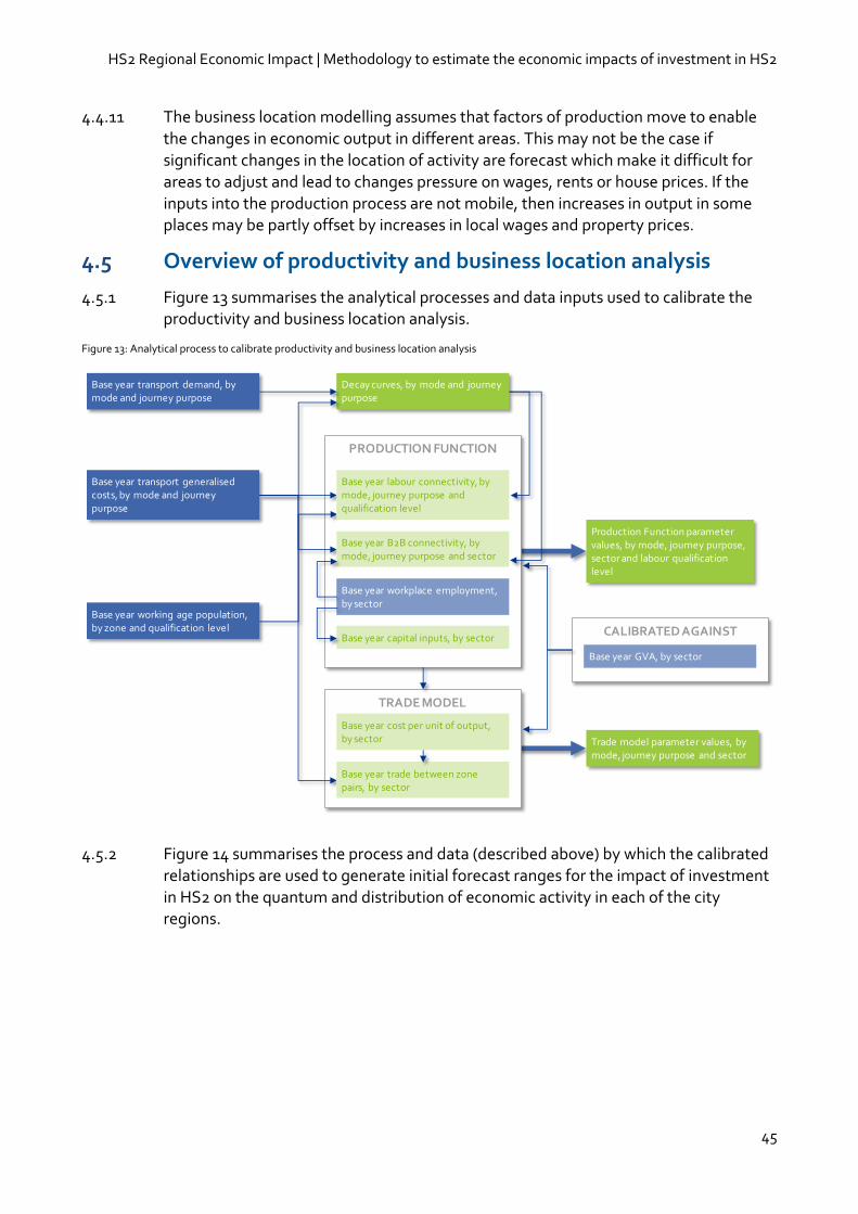
HS2 Regional Economic Impact | Methodology to estimate the economic impacts of investment in HS2
45
4.4.11 The business location modelling assumes that factors of production move to enable
the changes in economic output in different areas. This may not be the case if significant changes in the location of activity are forecast which make it difficult for areas to adjust and lead to changes pressure on wages, rents or house prices. If the inputs into the production process are not mobile, then increases in output in some places may be partly offset by increases in local wages and property prices.
4.5 Overview of productivity and business location analysis
4.5.1 Figure 13 summarises the analytical processes and data inputs used to calibrate the productivity and business location analysis.
Figure 13: Analytical process to calibrate productivity and business location analysis
4.5.2 Figure 14 summarises the process and data (described above) by which the calibrated relationships are used to generate initial forecast ranges for the impact of investment in HS2 on the quantum and distribution of economic activity in each of the city regions.
TRADE MODEL
PRODUCTION FUNCTION
Base year transport generalised costs, by mode and journey purpose
Base year working age population, by zone and qualification level
Base year labour connectivity, by mode, journey purpose and qualification level
Decay curves, by mode and journey purpose
Base year workplace employment, by sector
Base year B2B connectivity, by mode, journey purpose and sector
Base year capital inputs, by sector
Base year cost per unit of output, by sector
Base year trade between zone pairs, by sector
Production Function parameter values, by mode, journey purpose, sector and labour qualification level
Trade model parameter values, by mode, journey purpose and sector
Base year transport demand, by mode and journey purpose
CALIBRATED AGAINST
Base year GVA, by sector
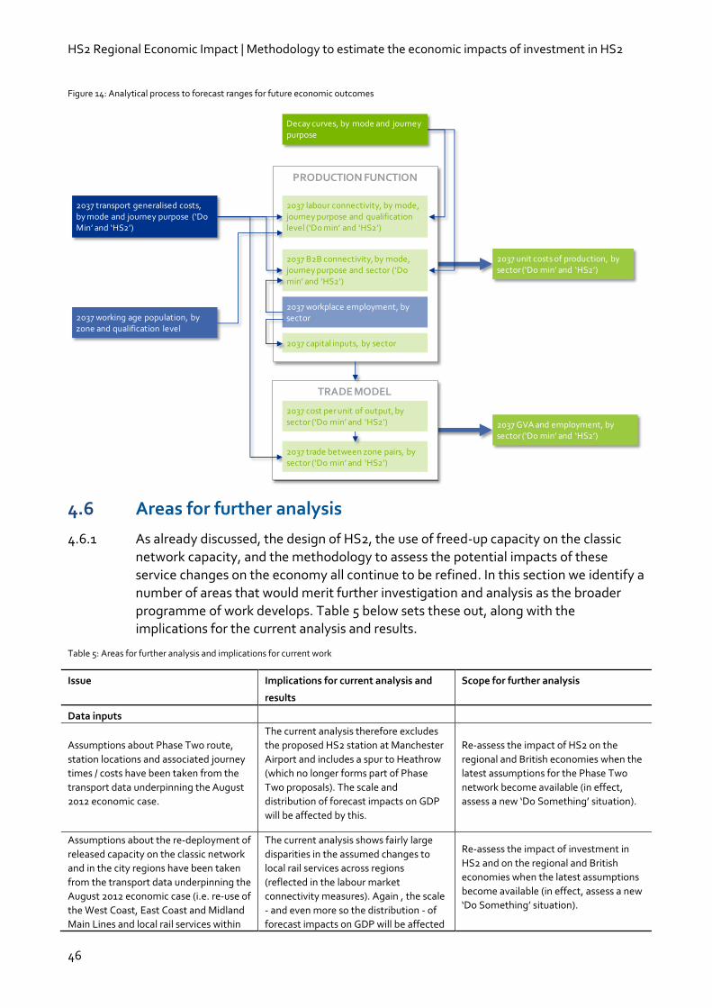
HS2 Regional Economic Impact | Methodology to estimate the economic impacts of investment in HS2
46
Figure 14: Analytical process to forecast ranges for future economic outcomes
4.6 Areas for further analysis
4.6.1 As already discussed, the design of HS2, the use of freed-up capacity on the classic network capacity, and the methodology to assess the potential impacts of these
service changes on the economy all continue to be refined. In this section we identify a number of areas that would merit further investigation and analysis as the broader programme of work develops. Table 5 below sets these out, along with the implications for the current analysis and results.
Table 5: Areas for further analysis and implications for current work
Issue Implications for current analysis and
results
Scope for further analysis
Data inputs
Assumptions about Phase Two route,
station locations and associated journey
times / costs have been taken from the
transport data underpinning the August
2012 economic case.
The current analysis therefore excludes
the proposed HS2 station at Manchester
Airport and includes a spur to Heathrow
(which no longer forms part of Phase
Two proposals). The scale and
distribution of forecast impacts on GDP
will be affected by this.
Re-assess the impact of HS2 on the
regional and British economies when the
latest assumptions for the Phase Two
network become available (in effect,
assess a new ‘Do Something’ situation).
Assumptions about the re-deployment of
released capacity on the classic network
and in the city regions have been taken
from the transport data underpinning the
August 2012 economic case (i.e. re-use of
the West Coast, East Coast and Midland
Main Lines and local rail services within
The current analysis shows fairly large
disparities in the assumed changes to
local rail services across regions
(reflected in the labour market
connectivity measures). Again , the scale
- and even more so the distribution - of
forecast impacts on GDP will be affected
Re-assess the impact of investment in
HS2 and on the regional and British
economies when the latest assumptions
become available (in effect, assess a new
‘Do Something’ situation).
TRADE MODEL
PRODUCTION FUNCTION
2037 transport generalised costs, by mode and journey purpose (‘Do Min’ and ‘HS2’)
2037 working age population, by zone and qualification level
2037 labour connectivity, by mode, journey purpose and qualification level (‘Do min’ and ‘HS2’)
Decay curves, by mode and journey purpose
2037 workplace employment, by sector
2037 B2B connectivity, by mode, journey purpose and sector (‘Do min’ and ‘HS2’)
2037 capital inputs, by sector
2037 cost per unit of output, by sector (‘Do min’ and ‘HS2’)
2037 trade between zone pairs, by sector (‘Do min’ and ‘HS2’)
2037 unit costs of production, by sector (‘Do min’ and ‘HS2’)
2037 GVA and employment, by sector (‘Do min’ and ‘HS2’)

HS2 Regional Economic Impact | Methodology to estimate the economic impacts of investment in HS2
47
Issue Implications for current analysis and
results
Scope for further analysis
city regions). by these assumptions. If ongoing work
on service patterns improves the quality
of local rail networks, then this could
increase the benefits of the scheme.
The data representing the distribution of
the population and economic activity
across Britain in the 2037 ‘Do Minimum’
situation has been taken from DfT
assumptions (‘Wider Impacts’ Dataset).
Areas across the country, including those
city regions with an HS2 station, are
likely to have their own view on the
distribution of activity in 2037 (before
investment in HS2 goes ahead) and thus
whether DfT assumptions are an
appropriate representation of their area.
Substantial differences from what has
been assumed could affect the
distribution of forecast impacts on GDP.
Further work to investigate the scale of
differences between DfT’s central
forecasts of 2037 ‘Do Minimum’ and
those locally. From this sensitivity
analysis could be undertaken (with an
alternative view of the Do Minimum
distribution of activity).
Methodology
The analysis is based on four separate
measures of connectivity and uncertainty
remains about their relative importance
Although overall the findings are in line
with other studies, uncertainty remains
about the relative importance of the
different connectivity measures.
Alternative approaches include
developing aggregate measure of
connectivity or using further statistical
techniques to address the correlation
between them.
Composite measures of connectivity
across modes could be created either
through a 'logsum' approach or by
demand weighting the generalised costs,
while new statistical work would need to
be supported by more detailed datasets
of the production characteristics of
individual firms.
The distance decay formulation is based
on observed travel patterns. Other
formulations are possible.
Alternative formulations could change
the impacts on productivity if they
systematically affected the modelled
changes in connectivity. For example,
formulations in which shorter trips are
more significant will tend to increase the
importance of local service changes.
Sensitivity testing could be expanded to
include different decay formulations,
including those recommended in the
appraisal of Wider Impacts within
welfare cost-benefit analysis.
Omission of variables from the
production function
The current analysis specifies a
production function with only labour and
capital as inputs to the production
process. It does not separately identify
other factors of production, such as land.
The production function analysis also
excludes other factors which could
influence productivity, such as the
natural advantage of locations (e.g.
being located on the coast).
Further work is needed to determine
whether this could be biasing the current
analysis upwards or downwards. The
availability of data to further
disaggregate the production function
would need to be investigated, e.g. the
extent to which Rateable Value data for
non-domestic properties could be used
at the zone level.
Analysis of only four aggregate business
sectors (construction; manufacturing;
producer services; and consumer
services).
Whilst the four sectors assessed
represent around two-thirds of the
economy, the level of aggregation does
not allow us to understand how the
production function and competitive
effects, and thus the influence of
connectivity on production/output, differ
Further work is needed to determine
whether this could be biasing the current
analysis upwards or downwards. It would
first be necessary to determine whether
consistent, independent and sufficiently
disaggregate data could be made
available to allow the analysis to be

HS2 Regional Economic Impact | Methodology to estimate the economic impacts of investment in HS2
48
Issue Implications for current analysis and
results
Scope for further analysis
within these sectors. based on a more detailed disaggregation
of the relevant parts of the economy (i.e.
a larger number of business sectors).
Absence of labour market dynamics.
The current analysis does not capture the
potential response of people to
incentives associated with better job
opportunities and/or higher wages
associated with improvements in
connectivity. This is likely to understate
the potential impact of investment in
HS2 on the economy, as increased labour
force participation (i.e. increased
employment) has not yet been captured.
Labour market dynamics should be
incorporated into the core approach.
This would ideally be fully integrated into
the current analysis (which would move
it towards a general equilibrium
approach). Alternatively, a separate
piece of analysis could be undertaken,
drawing on approaches established
elsewhere.
Feedback effects from business
relocation and competition between
areas.
Competition in itself is likely to be a
driver of business efficiency (i.e. in terms
of driving costs down) and hence
productivity (with and without business
relocation). The absence of these
impacts from the current analysis is likely
to understate the potential impact of
investment in HS2 on the economy.
In addition, the current analysis does not
assess the second-round productivity
impacts (and wage impacts) of
businesses being concentrated in more
productive areas after location effects.
This is again likely to understate the
potential impact of investment in HS2.
However, the potential negative
feedback effects are also excluded, such
as increased highway congestion and rail
crowding in those areas experiencing
increased economic activity, though
these are expected to be marginal
relative to the potential positive
feedback effects.
These feedback effects should be
incorporated into the core approach.
This would ideally be fully integrated into
the current analysis (which would move
it towards a general equilibrium
approach).
Zero-sum game assumption for
employment impacts
The current analysis does not forecast
net increases in employment at the
national level. This is likely to understate
the potential impact of investment in
HS2 on the economy.
In part linked to the issue of labour
market dynamics, a more detailed
assessment of employment impacts
should be incorporated into the core
approach. This would look to include
increased labour force participation in
response to higher wages (as above),
international migration, and potentially
other employment impacts which would
break the assumption of full-
employment in the long term.
Exclusion of both international
connectivity and international trade.
The current analysis does not capture
changes in international trade which may
be brought about by investment in HS2,
both in terms of providing improved
connections to airports (which act as
gateways for international connectivity)
and improving the British economy’s
Further work would be needed to
investigate potential data sources for
expanding the core approach to include
this international dimension.

HS2 Regional Economic Impact | Methodology to estimate the economic impacts of investment in HS2
49
Issue Implications for current analysis and
results
Scope for further analysis
competitive position in international
markets (all else being equal) by
becoming relatively more productive.
This is likely to understate the potential
impact of investment in HS2 on the
economy.
The current analysis assumes that
changes in transport connectivity cause
changes in productivity rather than the
other way around
While this assumption is common in
other academic work in this area, it is
very difficult to prove because time
series datasets are not available. Where
time series data is available some other
studies have been able to detect a causal
link between transport and infrastructure
investment and economic output,
however the transferability of these
results is uncertain.
If causality does run in both directions
then the results of our analysis could be
overstated.
It is unlikely that further work will be able
to definitively answer this question
without a significant improvement in the
data available on transport generalised
costs. This would need a significant
effort to examine historic transport
systems and economic patterns.
Freight impacts.
Whilst the current analysis includes an
assessment of car connectivity, it does
not specifically look at connectivity for
road freight or rail freight. The absence
of rail freight impacts in particular is
likely to understate the forecast impacts
on GDP brought about by investment in
HS2, but in particular the freed-up
capacity on the classic network, which
could be used for rail freight.
Further work is needed to investigate
whether sufficiently comprehensive and
consistent generalised cost data exists to
separately identify the impacts of
freight. (This would require appropriate
data for both the base year calibration
and 2037 'Do Minimum' and 'Do
Something'.)

HS2 Regional Economic Impact | Results
50
5 Results 5.1 Productivity impacts for the British economy
5.1.1 In this section of the report, we set out the potential impact on the British economy resulting from the improved connectivity and hence increased productivity brought about by investment in HS2. In Section 5.2 we set out how this forecast change in economic output could be distributed across Great Britain.
5.1.2 As set out in Table 6, our forecasts suggest that investment in HS2 could potentially generate £15 billion a year in productivity gains for the British economy in 2037 (2013 prices).
Table 6: Total annual productivity impacts for Great Britain in 2037 after investment in HS2 (2013 prices)
GDP impact per year
Total impact for GB economy £15 billion
5.1.3 Our approach makes it possible to determine how changes in the different forms of connectivity make up the estimated £15 billion impact. Table 7 below provides a breakdown of the possible impact on the British economy by rail and car connectivity to businesses and labour markets.
Table 7: Total annual productivity impacts for Great Britain by source of connectivity in 2037 after investment in HS2 (2013 prices)
GDP impact per year*
Total impact for GB economy £15 billion
Of which results from:
Rail connectivity to businesses £13 billion
Rail connectivity to labour £1 billion
Car connectivity (to labour and businesses) £0.2 billion
*Note: totals may not sum due to rounding
5.1.4 Improvements in rail connectivity to businesses is the largest driver of the forecast potential productivity gains for the GB economy – worth some £13 billion a year – as both HS2 and re-deployed classic network capacity provide a step-change in long-distance rail services, both on and off the proposed HS2 network.
5.1.5 Improvements in rail connectivity to labour account for a small proportion of the overall impact, totalling around £1 billion per year, as the service patterns assessed do not introduce significant changes to shorter-distance rail commuter services.
5.1.6 Whilst improvements to rail services make up the majority of the total potential productivity gains, around £0.2 billion per year is attributable to reduced highway congestion as improvements to rail services prompt some road users to switch from road to rail. This is reflected in improvements in car connectivity (to both labour and businesses).
HS2 Regional Economic Impact | Results
51
Sensitivity testing
Relative importance of connectivity in driving productivity
5.1.7 In our core approach, the production function captures how variations in the efficiency of the productive process can be explained by variations in transport connectivity. Four measures of connectivity have been considered and included in a production function for each of the four business sectors.
5.1.8 However, the four connectivity measures are correlated with one another. While each of the connectivity variables shows a positive and statistically significant relationship with productivity when tested separately, due to the correlation between them, it has not been possible to directly estimate their relative importance using a statistical approach.
5.1.9 Our core approach has therefore been to constrain the sensitivity of productivity to
connectivity to the maximum observed impact for any individual variable, and then share this elasticity between the ‘competing’ connectivity measures. The relative importance of the four connectivity measures has been inferred from the statistical analysis that separately tested each individual measure's influence on productivity.
5.1.10 In aggregate, this approach reflects the observed sensitivity of productivity to connectivity. However, uncertainty remains about the relative importance of the individual connectivity measures. To reflect this uncertainty, we have undertaken sensitivity analysis that employs an alternative approach to deriving the relative importance of the connectivity measures. This sensitivity uses data on transport demand patterns to deduce the appropriate weighting between connectivity measures.
5.1.11 Estimates of the mode share of rail and car miles travelled have been derived from the National Travel Survey for business travel. This shows that in 2011, of the miles travelled on business trips by car and rail, 14.7% were by rail. No data is directly
available to examine how this mode share varies by business sector. However, information is available that describes the balance of costs spent on rail services and other land transport services for each sector. We have used this to adjust the mode shares to better reflect the travel behaviour of different sectors.
5.1.12 While data is available describing the number of trips and miles travelled by mode for both business and commuting trips, it is not clear that the volume of travel is a useful guide to the relative economic importance of commuting and business trips. We have therefore excluded measures of commuting connectivity from this sensitivity test.
5.1.13 The mode share of business trips is therefore used to apportion the same aggregate elasticity that is used in our central case between:
a measure of connectivity to other business by car; and
a measure of connectivity to other business by rail.
5.1.14 The table below provides the results of this sensitivity analysis. We have found that, by deriving the relative importance of connectivity for productivity according to mode share, investment in HS2 could potentially generate up to £8 billion per year in
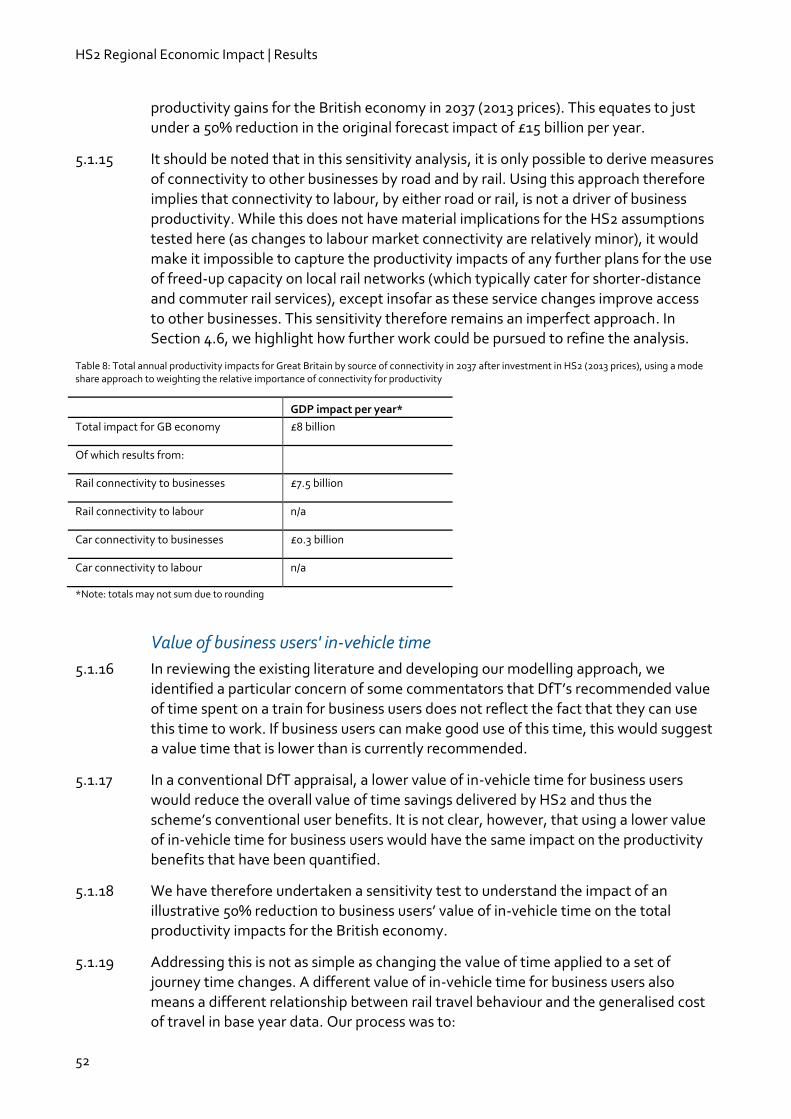
HS2 Regional Economic Impact | Results
52
productivity gains for the British economy in 2037 (2013 prices). This equates to just under a 50% reduction in the original forecast impact of £15 billion per year.
5.1.15 It should be noted that in this sensitivity analysis, it is only possible to derive measures of connectivity to other businesses by road and by rail. Using this approach therefore implies that connectivity to labour, by either road or rail, is not a driver of business productivity. While this does not have material implications for the HS2 assumptions tested here (as changes to labour market connectivity are relatively minor), it would make it impossible to capture the productivity impacts of any further plans for the use of freed-up capacity on local rail networks (which typically cater for shorter-distance and commuter rail services), except insofar as these service changes improve access to other businesses. This sensitivity therefore remains an imperfect approach. In Section 4.6, we highlight how further work could be pursued to refine the analysis.
Table 8: Total annual productivity impacts for Great Britain by source of connectivity in 2037 after investment in HS2 (2013 prices), using a mode share approach to weighting the relative importance of connectivity for productivity
GDP impact per year*
Total impact for GB economy £8 billion
Of which results from:
Rail connectivity to businesses £7.5 billion
Rail connectivity to labour n/a
Car connectivity to businesses £0.3 billion
Car connectivity to labour n/a
*Note: totals may not sum due to rounding
Value of business users' in-vehicle time
5.1.16 In reviewing the existing literature and developing our modelling approach, we identified a particular concern of some commentators that DfT’s recommended value of time spent on a train for business users does not reflect the fact that they can use this time to work. If business users can make good use of this time, this would suggest a value time that is lower than is currently recommended.
5.1.17 In a conventional DfT appraisal, a lower value of in-vehicle time for business users would reduce the overall value of time savings delivered by HS2 and thus the scheme’s conventional user benefits. It is not clear, however, that using a lower value of in-vehicle time for business users would have the same impact on the productivity benefits that have been quantified.
5.1.18 We have therefore undertaken a sensitivity test to understand the impact of an illustrative 50% reduction to business users’ value of in-vehicle time on the total productivity impacts for the British economy.
5.1.19 Addressing this is not as simple as changing the value of time applied to a set of journey time changes. A different value of in-vehicle time for business users also means a different relationship between rail travel behaviour and the generalised cost of travel in base year data. Our process was to:
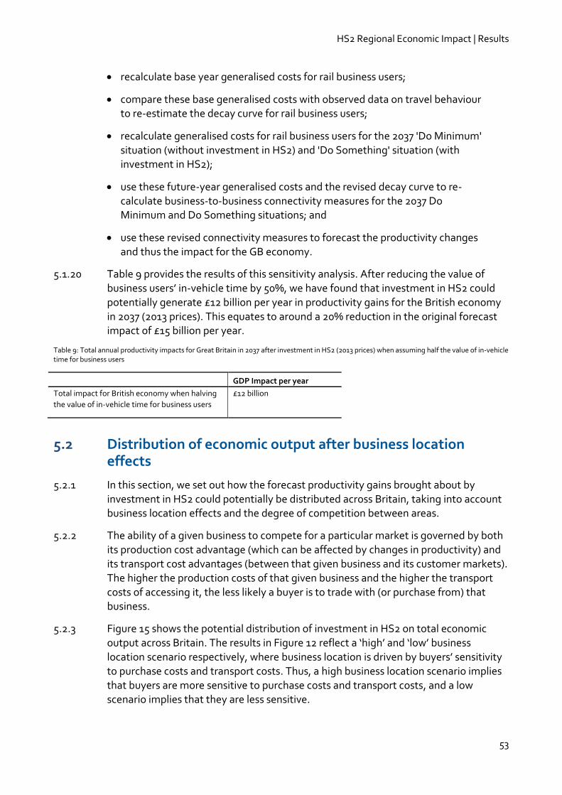
HS2 Regional Economic Impact | Results
53
recalculate base year generalised costs for rail business users;
compare these base generalised costs with observed data on travel behaviour to re-estimate the decay curve for rail business users;
recalculate generalised costs for rail business users for the 2037 'Do Minimum' situation (without investment in HS2) and 'Do Something' situation (with investment in HS2);
use these future-year generalised costs and the revised decay curve to re-calculate business-to-business connectivity measures for the 2037 Do Minimum and Do Something situations; and
use these revised connectivity measures to forecast the productivity changes and thus the impact for the GB economy.
5.1.20 Table 9 provides the results of this sensitivity analysis. After reducing the value of business users’ in-vehicle time by 50%, we have found that investment in HS2 could potentially generate £12 billion per year in productivity gains for the British economy in 2037 (2013 prices). This equates to around a 20% reduction in the original forecast impact of £15 billion per year.
Table 9: Total annual productivity impacts for Great Britain in 2037 after investment in HS2 (2013 prices) when assuming half the value of in-vehicle time for business users
GDP Impact per year
Total impact for British economy when halving
the value of in-vehicle time for business users
£12 billion
5.2 Distribution of economic output after business location effects
5.2.1 In this section, we set out how the forecast productivity gains brought about by investment in HS2 could potentially be distributed across Britain, taking into account business location effects and the degree of competition between areas.
5.2.2 The ability of a given business to compete for a particular market is governed by both its production cost advantage (which can be affected by changes in productivity) and its transport cost advantages (between that given business and its customer markets). The higher the production costs of that given business and the higher the transport costs of accessing it, the less likely a buyer is to trade with (or purchase from) that business.
5.2.3 Figure 15 shows the potential distribution of investment in HS2 on total economic output across Britain. The results in Figure 12 reflect a ‘high’ and ‘low’ business location scenario respectively, where business location is driven by buyers’ sensitivity to purchase costs and transport costs. Thus, a high business location scenario implies that buyers are more sensitive to purchase costs and transport costs, and a low scenario implies that they are less sensitive.
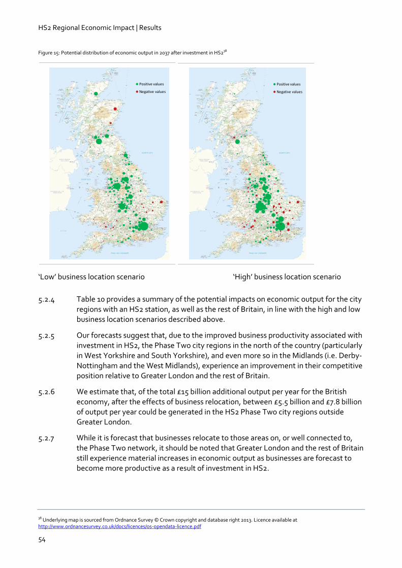
HS2 Regional Economic Impact | Results
54
Figure 15: Potential distribution of economic output in 2037 after investment in HS238
‘Low’ business location scenario ‘High’ business location scenario
5.2.4 Table 10 provides a summary of the potential impacts on economic output for the city regions with an HS2 station, as well as the rest of Britain, in line with the high and low business location scenarios described above.
5.2.5 Our forecasts suggest that, due to the improved business productivity associated with investment in HS2, the Phase Two city regions in the north of the country (particularly in West Yorkshire and South Yorkshire), and even more so in the Midlands (i.e. Derby-Nottingham and the West Midlands), experience an improvement in their competitive position relative to Greater London and the rest of Britain.
5.2.6 We estimate that, of the total £15 billion additional output per year for the British
economy, after the effects of business relocation, between £5.5 billion and £7.8 billion of output per year could be generated in the HS2 Phase Two city regions outside Greater London.
5.2.7 While it is forecast that businesses relocate to those areas on, or well connected to,
the Phase Two network, it should be noted that Greater London and the rest of Britain still experience material increases in economic output as businesses are forecast to become more productive as a result of investment in HS2.
38 Underlying map is sourced from Ordnance Survey © Crown copyright and database right 2013. Licence available at http://www.ordnancesurvey.co.uk/docs/licences/os-opendata-licence.pdf
Positive values
Negative values
Positive values
Negative values
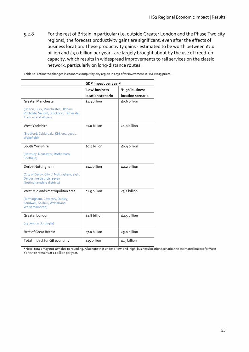
HS2 Regional Economic Impact | Results
55
5.2.8 For the rest of Britain in particular (i.e. outside Greater London and the Phase Two city
regions), the forecast productivity gains are significant, even after the effects of business location. These productivity gains - estimated to be worth between £7.0 billion and £5.0 billion per year - are largely brought about by the use of freed-up capacity, which results in widespread improvements to rail services on the classic network, particularly on long-distance routes.
Table 10: Estimated changes in economic output by city region in 2037 after investment in HS2 (2013 prices)
GDP impact per year*
‘Low’ business
location scenario
‘High’ business
location scenario
Greater Manchester
(Bolton, Bury, Manchester, Oldham, Rochdale, Salford, Stockport, Tameside, Trafford and Wigan)
£1.3 billion £0.6 billion
West Yorkshire
(Bradford, Calderdale, Kirklees, Leeds, Wakefield)
£1.0 billion £1.0 billion
South Yorkshire
(Barnsley, Doncaster, Rotherham, Sheffield)
£0.5 billion £0.9 billion
Derby-Nottingham
(City of Derby, City of Nottingham, eight Derbyshire districts, seven Nottinghamshire districts)
£1.1 billion £2.2 billion
West Midlands metropolitan area
(Birmingham, Coventry, Dudley, Sandwell, Solihull, Walsall and Wolverhampton)
£1.5 billion £3.1 billion
Greater London
(33 London Boroughs)
£2.8 billion £2.5 billion
Rest of Great Britain £7.0 billion £5.0 billion
Total impact for GB economy £15 billion £15 billion
*Note: totals may not sum due to rounding. Also note that under a 'low' and 'high' business location scenario, the estimated impact for West Yorkshire remains at £1 billion per year.
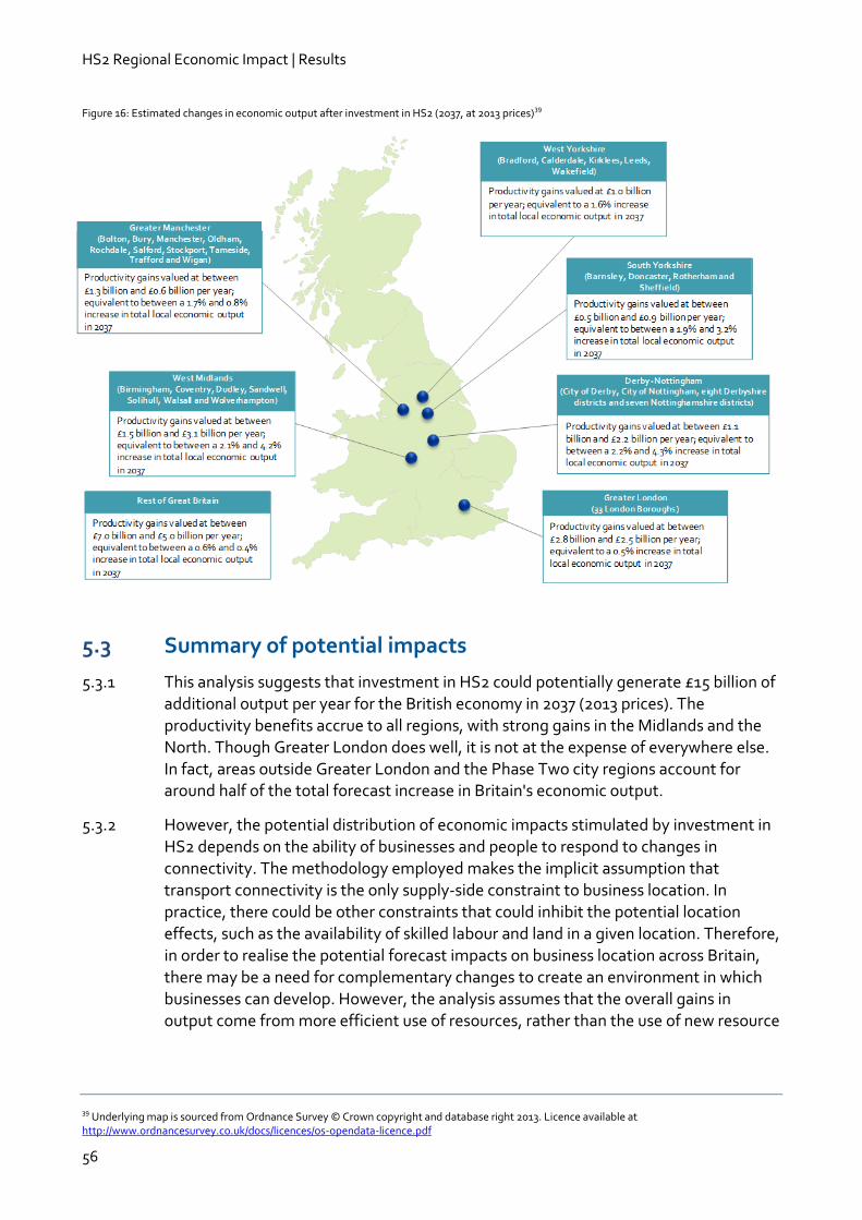
HS2 Regional Economic Impact | Results
56
Figure 16: Estimated changes in economic output after investment in HS2 (2037, at 2013 prices)39
5.3 Summary of potential impacts
5.3.1 This analysis suggests that investment in HS2 could potentially generate £15 billion of additional output per year for the British economy in 2037 (2013 prices). The productivity benefits accrue to all regions, with strong gains in the Midlands and the
North. Though Greater London does well, it is not at the expense of everywhere else. In fact, areas outside Greater London and the Phase Two city regions account for around half of the total forecast increase in Britain's economic output.
5.3.2 However, the potential distribution of economic impacts stimulated by investment in HS2 depends on the ability of businesses and people to respond to changes in connectivity. The methodology employed makes the implicit assumption that transport connectivity is the only supply-side constraint to business location. In practice, there could be other constraints that could inhibit the potential location effects, such as the availability of skilled labour and land in a given location. Therefore,
in order to realise the potential forecast impacts on business location across Britain, there may be a need for complementary changes to create an environment in which businesses can develop. However, the analysis assumes that the overall gains in output come from more efficient use of resources, rather than the use of new resource
39 Underlying map is sourced from Ordnance Survey © Crown copyright and database right 2013. Licence available at http://www.ordnancesurvey.co.uk/docs/licences/os-opendata-licence.pdf

HS2 Regional Economic Impact | Results
57
inputs, so the increased need for investment in areas that businesses move to is balanced by a reduced need for such investment in areas that they move from.
5.3.3 It is also important to recognise that these results are considered the first step in assessing the impacts of investment in HS2 on the British economy and the distribution of total economic output across the country. As Section 4.6 points out, there are a number of areas that merit further analysis to strengthen the analytical approach and the scope for addressing these continues to be developed. Along with the methodology, the design of HS2 and use of freed-up capacity on the classic network continue to be refined; any changes to the August 2012 economic case service assumptions that have been assessed here would warrant further assessment. In this sense, the results presented should be treated as provisional.
HS2 Regional Economic Impact | Technical appendices
58
6 Technical appendices 6.1 Key assumptions and data inputs
Introduction
6.1.1 This appendix provides an overview of the key assumptions made in the analysis and all the data sources used. These assumptions and data sources, and their use, are described further in Sections 6.2 and 6.3.
Key assumptions
6.1.2 The key assumptions in the analysis can be grouped into five main themes:
1. The UK’s geography and strategic transport network can be reasonably represented by the data sourced from the PLANET Long Distance model:
Dividing the UK into 235 zones for the purpose of modelling the impacts of investment in HS2 does not introduce a systematic bias into the analysis.
The generalised costs of travel derived from the PLANET Long Distance (PLD)
model appropriately measure the difficulty of strategic transport journeys within the UK relevant to the analysis of investment in HS2.
2. Connectivity provided by the transport system can be measured:
The connectivity offered by the transport system can be measured based on the
difficulty of travel to different places and the ‘opportunities’ available to businesses in those places.
The importance of access to an opportunity declines as the difficulty of accessing it increases and these relationships (decay curves) can be captured empirically through observed travel patterns.
3. Business behaviour is influenced by the connectivity that the transport system offers:
Total factor productivity in different business sectors can be influenced by transport connectivity (either through improved opportunities for specialisation, through the spread of knowledge and best practice, through better matching of buyers and sellers, or some other process).
The way that firms are able to turn inputs into outputs can be captured empirically based on their inputs of labour and capital and on transport connectivity measures.
Systematic bias is not introduced by excluding other inputs in the production process, such as land, which are not captured by the analysis.
Other factors that may affect this production process (such as differences in
climate, the natural advantage of locations, public investment levels, etc.) do not introduce a systematic bias into our analysis of the impact of transport connectivity on firms’ output.

HS2 Regional Economic Impact | Technical appendices
59
Transport connectivity causes changes in productivity rather than productivity
causing changes in transport connectivity.
The market share of different locations is partly determined by their production cost advantage and by the transport costs of selling to different markets.
4. Other economic effects do not systematically bias the analysis:
The impacts of the project on freight transport (for example, improved rail freight or more reliable road freight due to reduced road congestion) which have been excluded from the analysis do not cause systematic bias.
Changes in productivity and competitiveness that could influence international
trade, which may be brought about by investment in HS2 and which have been excluded from the analysis, do not systematically bias the results (these have been excluded from the analysis).
‘Second round’ or ‘feedback’ effects from changes in business behaviour and location (for example, increased concentration of business in the Phase Two city regions) do not systematically bias the analysis. For example, changes in the physical concentration of businesses could further increase agglomeration.
Any induced changes in wages and the prices of goods do not have a systematic
bias on the results. (Local productivity changes assume no changes in the inputs required to produce them, but changes in the location of production are expected to lead to increased employment in some areas and reduced employment in others.)
5. Economic forecasts of the future are within a reasonable range and key relationships will persist into the future:
Forecasts of economic output and employment in different business sectors which
have been drawn from government sources reflect reasonable long term future growth trends.
Forecast for transport demand which are used in the PLD model are a reasonable reflection of future transport demand. (These influence the crowding benefits in our analysis which are responsible for around £3 billion of the assessed benefits.)
Empirical relationships between transport connectivity and business behaviour persist in the future.

HS2 Regional Economic Impact | Technical appendices
60
List of data sources
Table 11: Complete list of data sources used in the analysis
Source Data Units How has it been used?
PLANET Long
Distance Model
Data representing
the generalised
costs of travel
between different
model zones in 2010
and 2037
£, in 2010 prices Used in the measurement of transport connectivity and
the representation of the costs of trade between different
locations.
Transport demand
data between model
zones in 2010
Person trips Used to observe the patterns of trip making by
generalised cost, which are used to calculate the decay
curves that are used in the calculation of transport
connectivity.
Plant North Model Transport demand
data between model
zones in 2010
Person trips Used to in-fill data gaps in the demand data drawn from
the PLD model
DfT Wider Impacts
Dataset
Workplace
employment by
sector by district
Persons in
employment
Used in the calculations for 2010 and 2037 of:
- measures of connectivity to businesses;
- estimates of intermediate demand for products and
services by businesses in different model zones; and
- labour inputs to the production function analysis
(including quality adjusted measure).
Gross Domestic
Product by sector
and local authority
district
£, 2010 prices Used to calculate total economic output by sector and
model zone in 2010 and 2037.
Average wage by
sector and district
£, 2010 prices Used to calculate the:
- total wage costs in each model zone in 2010 and 2037;
and
- total household expenditure in different model zones.
Census 2011 Residence based
population of
working age by skill
level
Persons Used in the calculations for 2010 and 2037 of measures of
connectivity to labour.
DfT National Trip
End Model v 6.2
Residential
population growth
rates
% changes over time Used to provide exogenous forecasts of future population
distribution which is used in the calculation of access to
labour in 2037.
HM Treasury Input-
output supply and
use table 2010
Expenditure by
businesses in
different sectors on
different products
and services
£, 2010 prices Used to estimate intermediate consumption of goods and
services by businesses by model zone.
Expenditure by
households on
different products
and services
Used to estimate:
- household consumption of goods and services by
households by model zone; and
- transport costs by road and rail by business sector which

HS2 Regional Economic Impact | Technical appendices
61
Source Data Units How has it been used?
is used in the calibration of the business location model.
National Travel
Survey
Business trips by
road and rail
Person trips Used to estimate the number of business trips per £ of
output in each business sector which is used in the
calibration of the business location model.
HS2 Regional Economic Impact | Technical appendices
62
6.2 Calculating connectivity
Introduction
6.2.1 This appendix describes the data and approach that we have taken to:
derive generalised costs of travel between different locations; and
develop measures of the connectivity provided by the transport system in these locations.
6.2.2 We explain the assumptions that have been made to correct for omissions, outliers and errors observed in the input generalised cost and demand data. We begin with an overview of the model geography, segmentation and time periods examined.
Geography, segmentation and time
6.2.3 The calculation of generalised cost is based on information extracted from the PLD model provided by HS2 Ltd. A map of the 235 PLD model zones is shown in Figure 17.
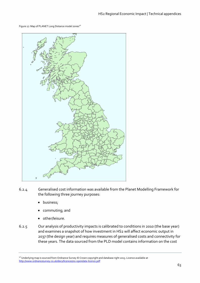
HS2 Regional Economic Impact | Technical appendices
63
Figure 17: Map of PLANET Long Distance model zones40
6.2.4 Generalised cost information was available from the Planet Modelling Framework for the following three journey purposes:
business;
commuting; and
other/leisure.
6.2.5 Our analysis of productivity impacts is calibrated to conditions in 2010 (the base year) and examines a snapshot of how investment in HS2 will affect economic output in 2037 (the design year) and requires measures of generalised costs and connectivity for these years. The data sourced from the PLD model contains information on the cost
40 Underlying map is sourced from Ordnance Survey © Crown copyright and database right 2013. Licence available at http://www.ordnancesurvey.co.uk/docs/licences/os-opendata-licence.pdf
HS2 Regional Economic Impact | Technical appendices
64
and demand for trips between the 235 PLD zones for the base year, 2010, as well as
forecasts for the year 2037 under both ‘Do Minimum’ (DM) and ‘Do Something’ (DS) scenarios.
6.2.6 All required socio-economic data was collected for the base year 2010. Where data was only available for a year close to 2010, the closest available dataset was used and re-based for 2010, as explained below. The DfT’s Wider Impacts Dataset, which forms the basis for much of our analysis, provides data for 2006 and for five-yearly intervals to 2041 and beyond. Data was derived from this for the design year of 2037 by linear interpolation.
The building blocks of connectivity
6.2.7 There are many ways on which measures of connectivity can be derived. These range from simple measurements such as the distance from a rail station or bus stop, to
more complex measures which quantify both the quality of transport provision and the opportunities it enables access to.
6.2.8 To assess the impacts of investment in HS2, we require a measure of connectivity that enables us to capture changes in rail journey times, service frequencies, costs, interchanges required, crowding levels and other features of the rail service. It must also be able to reflect the importance of the economic connection which is affected, for example by measuring the number of other businesses or potential employees that the connection allows access to.
6.2.9 Measurements of connectivity that are used in the economic literature tend to have three key elements:
information reflecting the difficulty of travel captured through distance or the
generalised cost of travel;
decay curve relationships describing how the importance of an opportunity decreases as the difficulty of travel increases; and
information about what is being accessed or connected to (for example, job opportunities, other businesses, etc.)
6.2.10 Most existing work that has attempted to draw links between transport, agglomeration and productivity has been based on a single measure of connectivity. These measures are usually based on the physical distance between places, rather than the difficulty of travel. Using distance is convenient because the information is readily available. It abstracts away from all other considerations of geography and transport supply.
6.2.11 Things become more complicated when the generalised cost of travel is introduced. There are many different generalised costs that can reflect travel between two places because generalised costs can differ by mode of transport, by user group and by the
purpose of travel. Similar considerations can also apply to distance-based measures because the appropriate distance to use is unclear. Should the relevant distance between Bristol and Cardiff be measured directly across the Bristol Channel or should a road or rail network distance be used - and if so, by which route?

HS2 Regional Economic Impact | Technical appendices
65
6.2.12 Thus, the construction of connectivity measures requires several judgments to be
made. If a single measure is constructed, the relative importance of each journey purpose, opportunity type or mode of transport is implicit in the weighting that it is given. If different measures are used, the relative importance of each can be made more explicit, but it can be difficult to disentangle the economic effects of the different measures.
6.2.13 There is no correct answer to these questions. In our analysis, we have chosen to derive separate measures of connectivity for different market segments, and attempted to understand their economic impacts separately. We recognise that this approach is one of many and that further work is needed to better understand the sensitivity of the analysis to different formulations of connectivity. The measures we have derived are constructed from three key building blocks:
the generalised costs of travel split by mode of transport and incorporating all of the available information about the time, cost and inconvenience of different elements of the journey;
decay curves that describe how opportunities become less significant as the generalised cost of travel increases; and
socio-economic data describing the opportunities that can be connected with
(including other businesses to trade with and pools of labour that could provide potential employees).
6.2.14 These three building blocks are described in more detail in the sections that follow.
Generalised costs
6.2.15 Table 12 provides a list of the information provided from the PLD model to calculate generalised costs of travel.
Table 12: Variables extracted from the PLANET Long Distance model used for the calculation of generalised costs
Description Unit
Car generalised costs component
Car in-vehicle time minutes
Fuel cost £/trip
Non-fuel cost £/trip
Total vehicle operating cost per person £/trip
Rail generalised costs component
In-vehicle time minutes
Auxiliary (access/egress) time minutes
Total wait time minutes
Boardings -
Additional time to reflect rail crowding minutes
Fare £
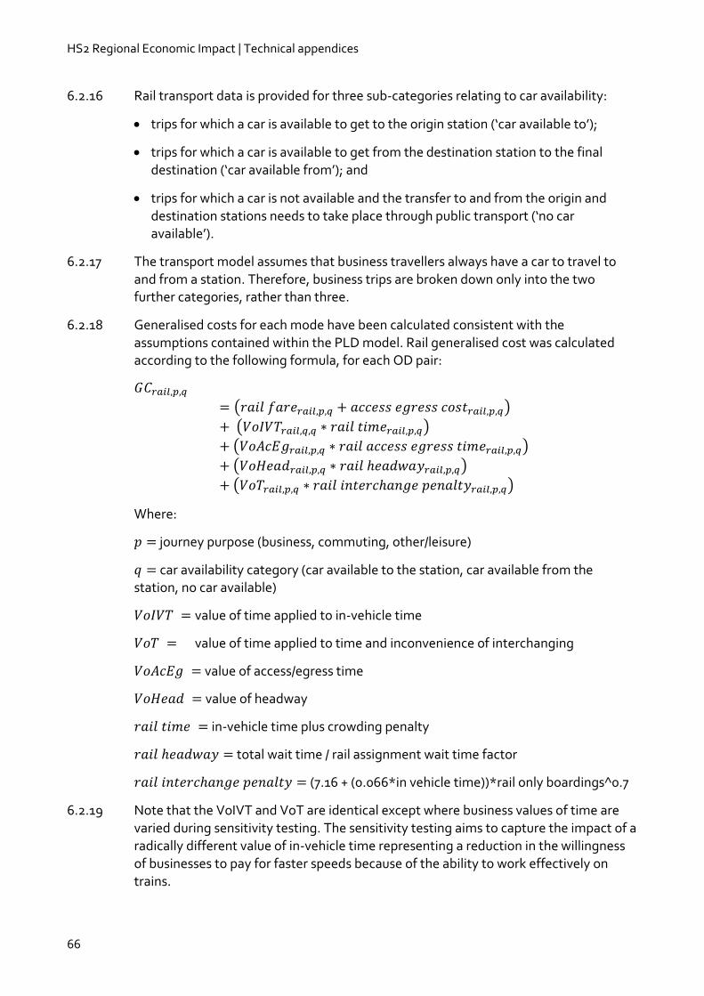
HS2 Regional Economic Impact | Technical appendices
66
6.2.16 Rail transport data is provided for three sub-categories relating to car availability:
trips for which a car is available to get to the origin station (‘car available to’);
trips for which a car is available to get from the destination station to the final destination (‘car available from’); and
trips for which a car is not available and the transfer to and from the origin and destination stations needs to take place through public transport (‘no car available’).
6.2.17 The transport model assumes that business travellers always have a car to travel to and from a station. Therefore, business trips are broken down only into the two further categories, rather than three.
6.2.18 Generalised costs for each mode have been calculated consistent with the
assumptions contained within the PLD model. Rail generalised cost was calculated according to the following formula, for each OD pair:
( )
( )
( )
( )
( )
Where:
journey purpose (business, commuting, other/leisure)
car availability category (car available to the station, car available from the station, no car available)
value of time applied to in-vehicle time
value of time applied to time and inconvenience of interchanging
value of access/egress time
value of headway
in-vehicle time plus crowding penalty
total wait time / rail assignment wait time factor
(7.16 + (0.066*in vehicle time))*rail only boardings^0.7
6.2.19 Note that the VoIVT and VoT are identical except where business values of time are varied during sensitivity testing. The sensitivity testing aims to capture the impact of a radically different value of in-vehicle time representing a reduction in the willingness of businesses to pay for faster speeds because of the ability to work effectively on trains.
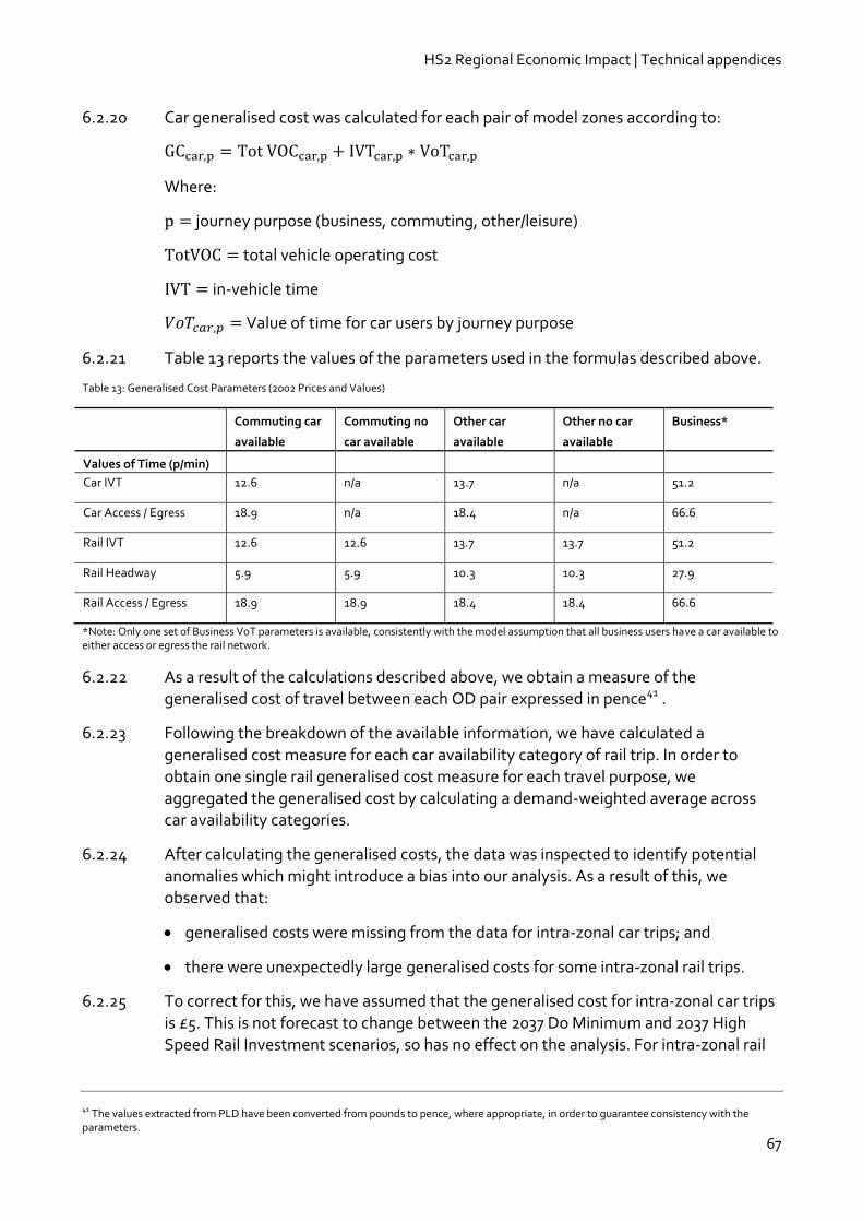
HS2 Regional Economic Impact | Technical appendices
67
6.2.20 Car generalised cost was calculated for each pair of model zones according to:
Where:
journey purpose (business, commuting, other/leisure)
total vehicle operating cost
in-vehicle time
Value of time for car users by journey purpose
6.2.21 Table 13 reports the values of the parameters used in the formulas described above.
Table 13: Generalised Cost Parameters (2002 Prices and Values)
Commuting car
available
Commuting no
car available
Other car
available
Other no car
available
Business*
Values of Time (p/min)
Car IVT 12.6 n/a 13.7 n/a 51.2
Car Access / Egress 18.9 n/a 18.4 n/a 66.6
Rail IVT 12.6 12.6 13.7 13.7 51.2
Rail Headway 5.9 5.9 10.3 10.3 27.9
Rail Access / Egress 18.9 18.9 18.4 18.4 66.6
*Note: Only one set of Business VoT parameters is available, consistently with the model assumption that all business users have a car available to either access or egress the rail network.
6.2.22 As a result of the calculations described above, we obtain a measure of the generalised cost of travel between each OD pair expressed in pence41 .
6.2.23 Following the breakdown of the available information, we have calculated a generalised cost measure for each car availability category of rail trip. In order to obtain one single rail generalised cost measure for each travel purpose, we aggregated the generalised cost by calculating a demand-weighted average across car availability categories.
6.2.24 After calculating the generalised costs, the data was inspected to identify potential anomalies which might introduce a bias into our analysis. As a result of this, we observed that:
generalised costs were missing from the data for intra-zonal car trips; and
there were unexpectedly large generalised costs for some intra-zonal rail trips.
6.2.25 To correct for this, we have assumed that the generalised cost for intra-zonal car trips is £5. This is not forecast to change between the 2037 Do Minimum and 2037 High Speed Rail Investment scenarios, so has no effect on the analysis. For intra-zonal rail
41 The values extracted from PLD have been converted from pounds to pence, where appropriate, in order to guarantee consistency with the parameters.
HS2 Regional Economic Impact | Technical appendices
68
trips, we followed DfT guidance in WebTAG Unit 3.10.2 and assumed that, for each
zone, the generalised cost for an intra-zonal trip is equal to half the generalised cost of the trip to the nearest destination.
Decay curves: the importance of generalised cost
6.2.26 A measure of connectivity must capture how the importance of places attenuates as they become progressively more difficult to access. Thus, somewhere that is easy to access (other things being equal) should be counted more highly in a calculation of connectivity than places that are more difficult to access. Decay curves are used to describe how the importance of generalised cost declines as generalised costs increase.
6.2.27 Decay relationships could have different shapes. For example, it is possible to use a mathematical relationship such as a straight-line decay or an exponential decay. In our
analysis we base these relationships on observed patterns of travel to reflect how the volume of travel diminishes as the generalised costs increase. Demand data from the PLD model is used to develop an understanding of travel behaviour. This behaviour is used to derive decay curves which reflect how trip making declines as generalised costs increase. Systematic omissions in the demand data (for example, consistently missing data for short-distance trips) could bias this analysis. The following demand data was not present in the data extracted from the PLD model:
short-distance trips between some zones in the north of the country;
demand for trips with destination in the south of the country; and
demand for intra-zonal car trips.
6.2.28 Missing demand data for short-distance trips within the north of the country was in-filled using data from the PLANET North Model. We used the information from this model to retrieve the demand for short-distance rail trips between 520 OD pairs in the Northern regions, which was missing in PLD. This provided a complete dataset of trip making to zones in the north of the country. The decay relationships were created on the basis of observed trip-making behaviour to destinations in the north of the country for which complete demand datasets were available to avoid potential bias introduced by missing demand data.
6.2.29 Further work could be undertaken to create a consistent set of demand data across the country and calibrate decay curves based on this. In particular, trip making to or from London may experience different behaviour from the rest of the UK. However, we expect that travel behaviour to the wide range of destinations that we have
captured will be broadly reflective of aggregate national travel behaviour. We therefore expect that this data constraint will not have a significant impact on the shape of the curves or on the subsequent analysis and findings.
6.2.30 Separate decay curves are produced for each travel mode and journey purpose. The decay curves used in the modelling are shown in Figure 18.
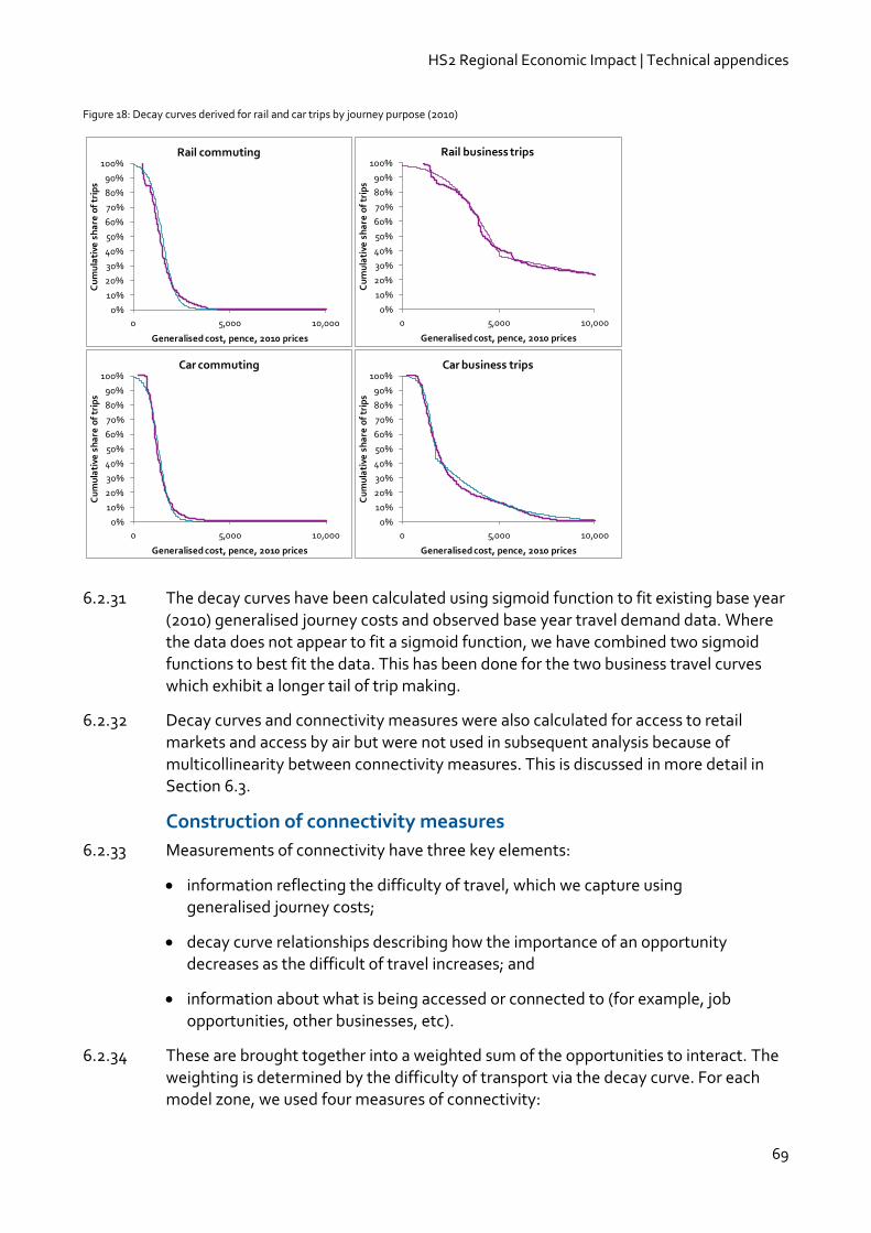
HS2 Regional Economic Impact | Technical appendices
69
Figure 18: Decay curves derived for rail and car trips by journey purpose (2010)
6.2.31 The decay curves have been calculated using sigmoid function to fit existing base year (2010) generalised journey costs and observed base year travel demand data. Where the data does not appear to fit a sigmoid function, we have combined two sigmoid functions to best fit the data. This has been done for the two business travel curves which exhibit a longer tail of trip making.
6.2.32 Decay curves and connectivity measures were also calculated for access to retail markets and access by air but were not used in subsequent analysis because of
multicollinearity between connectivity measures. This is discussed in more detail in Section 6.3.
Construction of connectivity measures
6.2.33 Measurements of connectivity have three key elements:
information reflecting the difficulty of travel, which we capture using generalised journey costs;
decay curve relationships describing how the importance of an opportunity decreases as the difficult of travel increases; and
information about what is being accessed or connected to (for example, job opportunities, other businesses, etc).
6.2.34 These are brought together into a weighted sum of the opportunities to interact. The weighting is determined by the difficulty of transport via the decay curve. For each model zone, we used four measures of connectivity:
0%
10%
20%
30%
40%
50%
60%
70%
80%
90%
100%
0 5,000 10,000
Cu
mu
lati
ve s
ha
re o
f tr
ips
Generalised cost, pence, 2010 prices
Rail commuting
0%
10%
20%
30%
40%
50%
60%
70%
80%
90%
100%
0 5,000 10,000
Cu
mu
lati
ve s
ha
re o
f tr
ips
Generalised cost, pence, 2010 prices
Rail business trips
0%
10%
20%
30%
40%
50%
60%
70%
80%
90%
100%
0 5,000 10,000
Cu
mu
lati
ve s
ha
re o
f tr
ips
Generalised cost, pence, 2010 prices
Car commuting
0%
10%
20%
30%
40%
50%
60%
70%
80%
90%
100%
0 5,000 10,000
Cu
mu
lati
ve s
ha
re o
f tr
ips
Generalised cost, pence, 2010 prices
Car business trips
HS2 Regional Economic Impact | Technical appendices
70
rail connectivity to labour;
rail connectivity to businesses;
car connectivity to labour; and
car connectivity to businesses.
6.2.35 To create the connectivity measures, we first select the transport data for the relevant transport mode and journey purpose segment. For example, rail connectivity to other businesses is calculated using rail generalised journey costs data, which is calculated based on the behaviour of rail business travellers. Next, we select the appropriate decay curve, which has been calibrated based on the behaviour of this group. We then select the appropriate data for what is being connected to. In the case of connectivity to businesses, we use data for workplace employment to reflect both the number and size of businesses in each area with which a business could potentially connect.
6.2.36 The socio-economic data has been aggregated to the geographical zone structure used by the PLD Model. These zones best correspond to local authority districts or
groups of local authority districts. The socio-economic data compilation therefore involves the collection of data at local authority district level where possible, and then mapping accordingly to the 235 zones defined in the PLD Model. Pre-2009 local authority districts, or collections of districts, map to PLD zones directly. PLD zone-level data was compiled by summing all of the local authority districts that belong to the PLD zone.
6.2.37 The DfT publishes socio-economic data which is intended to be used in the calculation of Wider Impacts within transport appraisal (the DfT’s Wider Impacts dataset). We have drawn heavily on this dataset in our analysis. It provides a measure of total
employment for each local authority district, which represents the total number of workplace jobs occupied in all industries. This data is organised by pre-2009 local authority district, and is therefore geographically compatible with the PLD zone structure. Data is available for 2006 and for five-year increments. Straight-line growth has been assumed in the five years from 2006 to 2011 to deduce 2010 employment levels and in the five years from 2036 to 2041 to deduce 2037 employment levels.
6.2.38 Census data provides population figures for England and Wales for the 16 to 64 age group. Data is available at local authority district level according to 2011 district boundaries. Census data was collected at district level, except for unitary authorities redrawn in 2009 (Wiltshire, Cheshire West and Chester, Cheshire East, County Durham, Wiltshire, Shropshire, Northumberland and Central Bedfordshire). Data for these authorities was collected at middle super output area level and then mapped to
the pre-2009 local authority areas by adding together the values of the respective middle super output areas. Scottish Census data was collected for 2001 and 2011 and interpolated to provide an estimate of population aged 16 to 65 in 2010 by Scottish district. Future-year forecasts for Scotland were estimated using population growth factors for the 16-64 age group as supplied in the National Trip End Model (NTEM) version 6.2.
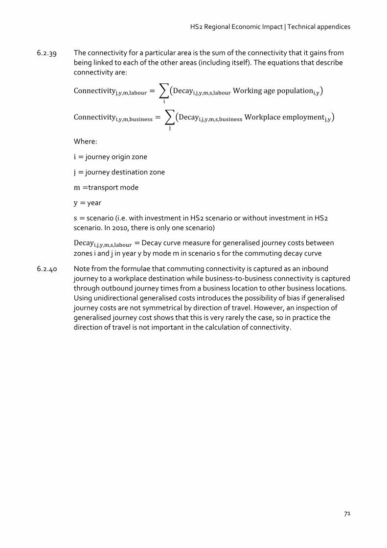
HS2 Regional Economic Impact | Technical appendices
71
6.2.39 The connectivity for a particular area is the sum of the connectivity that it gains from
being linked to each of the other areas (including itself). The equations that describe connectivity are:
∑( )
∑( )
Where:
journey origin zone
journey destination zone
transport mode
year
scenario (i.e. with investment in HS2 scenario or without investment in HS2 scenario. In 2010, there is only one scenario)
Decay curve measure for generalised journey costs between
zones i and j in year y by mode m in scenario s for the commuting decay curve
6.2.40 Note from the formulae that commuting connectivity is captured as an inbound journey to a workplace destination while business-to-business connectivity is captured through outbound journey times from a business location to other business locations. Using unidirectional generalised costs introduces the possibility of bias if generalised
journey costs are not symmetrical by direction of travel. However, an inspection of generalised journey cost shows that this is very rarely the case, so in practice the direction of travel is not important in the calculation of connectivity.
HS2 Regional Economic Impact | Technical appendices
72
6.3 Productivity and business location analysis
6.3.1 The analysis of productivity and business location impacts is undertaken in two stages.
Productivity model: First, we hypothesise that changes in transport connectivity can affect firm productivity. We then test this assumption using statistical analysis and use the findings to test how future changes in connectivity brought about by investment in HS2 could affect productivity. This model is calibrated using observed productivity in different sectors and locations.
Business location model: Second, we model the output and trade position of
different geographical areas as a function of both their ‘domestic’ productivity advantage and the transport costs of delivering goods or services to particular
geographic markets. With investment in HS2, connectivity changes affect the domestic productivity advantages of different places (from the productivity model) but transport costs between different markets also change enabling more efficient producing locations to increase their share of sales to other geographical areas. The business location model is calibrated using data on local productivity differentials, data on transport costs between different areas and the output of different areas. It is a zero-sum allocation model in which the market for goods and services in each zone is allocated between producing zones according to the strength of their trade position and does not forecast any further net changes in output.
6.3.2 These models are described in more detail below.
Production function
6.3.3 We have tested the hypothesis that transport connectivity can influence productivity by constructing a production function which describes how different areas convert labour and capital inputs into outputs. Statistical techniques have then been used to determine whether measured variations in transport connectivity affect the technical efficiency of the production process.
6.3.4 The analysis is undertaken by business sector. The breakdown used in this study is consistent with DfT’s Wider Impacts Dataset, which includes:
construction;
consumer services;
manufacturing; and
producer services.
6.3.5 These sectors do not represent the whole of the UK economy, omitting 36% of workplace employment. The agriculture sector, for example, is not included. The DfT42 provides a mapping of Standard Industrial Classification (SIC) codes to the four
42 Department for Transport, WebTAG, Unit 3.5.14: The Wider Impacts Sub-Objective.
HS2 Regional Economic Impact | Technical appendices
73
sectors for the 1992 Standard Industrial Classification (SIC92) of business activities.
However, data collected for 2010 is represented in the 2007 system of Standard Industrial Classifications (SIC07) and therefore do not map directly to the DfT’s Wider Impact sectors. We have used a mapping system between the two SIC codes to approximate, as far as possible, the map between SIC 2007 and the DfT’s Wider Impact sectors.
6.3.6 The production function has been estimated using data for the 235 model zones (excluding Pembrokeshire in West Wales, for which generalised cost measures and hence connectivity were not always available). Labour inputs are sourced from the DfT’s Wider Impacts dataset as described above. Wage data is not available by local authority and region, so has been constructed. The DfT’s Wider Impacts Dataset has wage data available over time by local authority, but not by business sector. The Annual Survey of Hours and Earnings (ASHE) provides data on annual gross pay by
business sector for the Standard Industrial Classifications 2007, but is available only at the geographic level of UK regions. Using the ASHE data, differences in pay from the all-sector average were calculated for the different sectors in each region. These differences were then applied to the district level data to estimate district level wages by sector. Due to data constraints, this was the best available method to approximate regional and sectoral differences in average pay.
6.3.7 The choice of the functional form of the production function has been dictated by available data. In particular, it has not been possible to independently construct local area level data for capital inputs and no such data exists in the public domain. Other studies have avoided this problem by either:
assuming that capital costs and labour costs are employed in fixed ratios, which has been supported by observed data; or
using data collected from the accounts of individual firms to examine their labour and capital costs directly.
6.3.8 We have adopted the first strategy and derived appropriate capital and labour cost ratios from national input output data. Since
where
total cost of production in zone i in sector s
labour input in zone i in sector s
wage in zone i in sector s
capital input in zone i in sector s
cost of capital
if the cost shares of labour and capital are given by α and 1- α respectively, then
(
)
HS2 Regional Economic Impact | Technical appendices
74
6.3.9 However, this assumption of fixed capital and labour cost shares and their
implementation within the Cobb-Douglas formulation implies constant returns to scale (excluding the impacts of connectivity on agglomeration) because a proportionate increase in both labour and capital inputs will result in an equal proportionate increase in output. This set of assumptions implies a Cobb-Douglas production technology described by:
where
Economic output in zone i
A parameter reflecting productivity
Labour input in zone i
Capital input in zone i
Share of input costs allocated to labour inputs
6.3.10 By taking the natural logarithm of both sides of this equation, the parameter α can be estimated within a linear equation:
( ) (
) , so
( ) ( ) ( ) ( )
6.3.11 We have assumed that if connectivity affects productivity, it does so by affecting total factor productivity rather than labour or capital productivity (a Hicks neutral impact). It therefore enters the production function through the productivity parameter A. Connectivity is introduced into the production function as follows:
( ) ( ) ( ) ( ) ( ) ( ) ( )
where
Productivity constant
Elasticity of productivity with respect to
Connectivity measure 1
6.3.12 Using this approach, differences in the different connectivity measures have the potential to either increase or decrease total factor productivity. This analysis has been undertaken by business sector for the four business sectors. Finally, we have
introduced flags in the modelling for Scotland and Wales and introduced constants for these countries to allow for specific unobserved factors that affect productivity that may differ by country. This reflects potential differences in planning, law, transport
policy, etc. Incorporating all of these factors, the final production function equation is given by:
( )
( ) ( ) ( )

HS2 Regional Economic Impact | Technical appendices
75
where
Business sector
Fixed productivity effect for Scotland
Scotland flag to identify which zones are in Scotland
Fixed productivity effect for Wales
Wales flag to identify which zones are in Wales
6.3.13 We have estimated this equation using various different measures of connectivity, including:
rail connectivity to labour;
rail connectivity to workplace employment;
car connectivity to labour; and
car connectivity to workplace employment.
6.3.14 Examination of the input connectivity data found that many of the measures of connectivity examined are correlated. This poses a significant challenge for the analysis and means that it is not possible to examine the productivity impacts of each within the same forecasting equation.
6.3.15 A potential approach to solving the problem of multicollinearity is to use instrumental variables. Such an approach would likely need to be based on more data, probably based on individual firm characteristics, and has not been possible within the
timescales of this study. Instead, we have examined the contribution of each connectivity variable in isolation and employed a different approach to avoid double counting between them, which is described below.
6.3.16 Table 14 shows the findings of the statistical analysis.
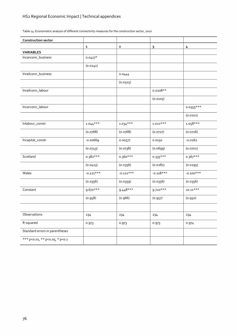
HS2 Regional Economic Impact | Technical appendices
76
Table 14: Econometric analysis of different connectivity measures for the construction sector, 2010
Construction sector
1 2 3 4
VARIABLES
lncarconn_business 0.0417*
(0.0241)
lnrailconn_business 0.0444
(0.0325)
lnrailconn_labour 0.0208**
(0.0105)
lncarconn_labour 0.0355***
(0.0102)
lnlabour_constr 1.044*** 1.034*** 1.022*** 1.058***
(0.0768) (0.0768) (0.0727) (0.0726)
lncapital_constr -0.00669 0.00577 0.0150 -0.0262
(0.0743) (0.0738) (0.0699) (0.0702)
Scotland 0.382*** 0.360*** 0.335*** 0.367***
(0.0413) (0.0356) (0.0281) (0.0295)
Wales -0.121*** -0.121*** -0.118*** -0.100***
(0.0356) (0.0359) (0.0356) (0.0356)
Constant 9.670*** 9.448*** 9.720*** 10.11***
(0.958) (0.966) (0.957) (0.950)
Observations 234 234 234 234
R-squared 0.973 0.973 0.973 0.974
Standard errors in parentheses
*** p<0.01, ** p<0.05, * p<0.1
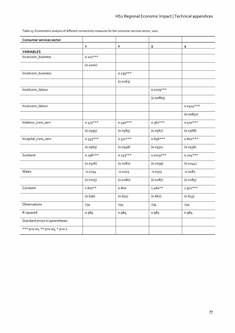
HS2 Regional Economic Impact | Technical appendices
77
Table 15: Econometric analysis of different connectivity measures for the consumer services sector, 2010
Consumer services sector
1 2 3 4
VARIABLES
lncarconn_business 0.111***
(0.0200)
lnrailconn_business 0.139***
(0.0263)
lnrailconn_labour 0.0279***
(0.00865)
lncarconn_labour 0.0414***
(0.00852)
lnlabour_cons_serv 0.475*** 0.450*** 0.361*** 0.410***
(0.0595) (0.0585) (0.0567) (0.0568)
lncapital_cons_serv 0.543*** 0.572*** 0.656*** 0.602***
(0.0563) (0.0548) (0.0531) (0.0536)
Scotland 0.196*** 0.153*** 0.0719*** 0.104***
(0.0326) (0.0282) (0.0239) (0.0244)
Wales -0.0254 -0.0203 -0.0373 -0.0182
(0.0275) (0.0280) (0.0287) (0.0285)
Constant 1.607** 0.800 1.460** 1.972***
(0.636) (0.651) (0.662) (0.653)
Observations 234 234 234 234
R-squared 0.984 0.984 0.983 0.984
Standard errors in parentheses
*** p<0.01, ** p<0.05, * p<0.1

HS2 Regional Economic Impact | Technical appendices
78
Table 16: Econometric analysis of different connectivity measures for the manufacturing sector, 2010
Manufacturing sector
1 2 3 4
VARIABLES
lncarconn_business 0.0323
(0.0252)
lnrailconn_business 0.0452
(0.0333)
lnrailconn_labour 0.0167
(0.0107)
lncarconn_labour 0.0263**
(0.0106)
lnlabour_manuf 0.581*** 0.579*** 0.562*** 0.592***
(0.0711) (0.0698) (0.0652) (0.0667)
lncapital_manuf 0.414*** 0.416*** 0.431*** 0.397***
(0.0693) (0.0676) (0.0630) (0.0649)
Scotland 0.278*** 0.268*** 0.240*** 0.263***
(0.0417) (0.0355) (0.0279) (0.0294)
Wales -0.106*** -0.104*** -0.107*** -0.0887**
(0.0344) (0.0345) (0.0333) (0.0345)
Constant 4.800*** 4.576*** 4.839*** 5.178***
(0.851) (0.850) (0.851) (0.862)
Observations 234 234 234 234
R-squared 0.973 0.973 0.973 0.974
Standard errors in parentheses
*** p<0.01, ** p<0.05, * p<0.1
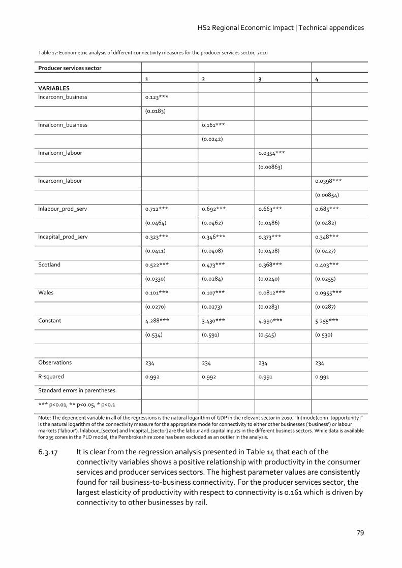
HS2 Regional Economic Impact | Technical appendices
79
Table 17: Econometric analysis of different connectivity measures for the producer services sector, 2010
Producer services sector
1 2 3 4
VARIABLES
lncarconn_business 0.123***
(0.0183)
lnrailconn_business 0.161***
(0.0242)
lnrailconn_labour 0.0354***
(0.00863)
lncarconn_labour 0.0398***
(0.00854)
lnlabour_prod_serv 0.712*** 0.692*** 0.663*** 0.685***
(0.0464) (0.0462) (0.0486) (0.0482)
lncapital_prod_serv 0.323*** 0.346*** 0.373*** 0.348***
(0.0411) (0.0408) (0.0428) (0.0427)
Scotland 0.522*** 0.473*** 0.368*** 0.403***
(0.0330) (0.0284) (0.0240) (0.0255)
Wales 0.101*** 0.107*** 0.0812*** 0.0955***
(0.0270) (0.0273) (0.0283) (0.0287)
Constant 4.288*** 3.430*** 4.990*** 5.255***
(0.534) (0.591) (0.545) (0.530)
Observations 234 234 234 234
R-squared 0.992 0.992 0.991 0.991
Standard errors in parentheses
*** p<0.01, ** p<0.05, * p<0.1
Note: The dependent variable in all of the regressions is the natural logarithm of GDP in the relevant sector in 2010. “ln[mode}conn_[opportunity]” is the natural logarithm of the connectivity measure for the appropriate mode for connectivity to either other businesses (‘business’) or labour markets (‘labour’). lnlabour_[sector] and lncapital_[sector] are the labour and capital inputs in the different business sectors. While data is available for 235 zones in the PLD model, the Pembrokeshire zone has been excluded as an outlier in the analysis.
6.3.17 It is clear from the regression analysis presented in Table 14 that each of the connectivity variables shows a positive relationship with productivity in the consumer services and producer services sectors. The highest parameter values are consistently found for rail business-to-business connectivity. For the producer services sector, the largest elasticity of productivity with respect to connectivity is 0.161 which is driven by connectivity to other businesses by rail.
HS2 Regional Economic Impact | Technical appendices
80
6.3.18 In the construction sector, different connectivity measures show different levels of
statistical significance, with access to labour by car significant at the 99% level and access to labour by rail significant at the 95% level. In the manufacturing sector, the only connectivity measure which has any statistical significance is the measure of connectivity to labour by car.
Testing for labour quality effects
6.3.19 We have also examined the implications of using an alternative measure of labour input to the production function which captures ‘quality adjusted’ labour, based on the observed occupational mix of workplace employment of model zones. To do this we derived an approach for weighting the labour input data taken from DfT’s Wider Impacts Dataset.
6.3.20 To derive weighting factors, data on the average wage by Standard Occupation
Classification 2010 (SOC2010) was taken from the Annual Population Survey. From these detailed definitions, data was aggregated to classifications of ‘high’ and ‘low’ occupational group43. A further breakdown by business sector, however, is not available from the survey data. This means it is not possible to determine whether, for example, ‘high’ occupations in Producer Services have a relatively higher wage than ‘high’ occupations in Manufacturing. We can only determine whether, on average (i.e. across all sectors), ‘high’ occupations are paid more/less than ‘low’ occupations. This data is only available at the regional level; therefore, we are able to understand whether ‘high’ occupations are paid more/less in one region compared to ‘high’ occupations in another, but we cannot determine this geographic variation at the local authority (and thus zone) level. Regional data was therefore used as a best proxy for deriving weighting factors for PLD zone data.
6.3.21 The average wage of ‘high’ and ‘low’ occupations by region was then compared to the average workplace wage by region (i.e. across all occupations) in order to derive a set of weighting factors by occupational group by region. For example, in the North West, ‘high’ occupations are paid 1.43 times more than the average worker, and ‘low’ occupations are paid 0.7 of the average wage.
6.3.22 Data on workplace employment by SOC2010 and broad business sector (defined as ‘Sections’ under the Standard Industrial Classification 2007) by region was then taken from the Annual Population Survey in order to understand the share of workers in ‘high’ and ‘low’ occupational groups by the four DfT business sectors. These regional shares, along with the regional weighting factors, were then applied to the labour input data for the relevant PLD zone (e.g. factors derived for the North West have been applied to the Manchester and Liverpool PLD zones).
6.3.23 The modelled elasticities are shown in Table 18 below, along with their comparators when no allowance has been made for labour quality.
43 The ‘high’ occupational group includes the three most senior occupations of the total nine classified under SOC2010. These are (i) Managers, directors and senior officials; (ii) Professional occupations; and (iii) Associate professional and technical occupations. The remaining six occupations under SOC2010 comprise the ‘low’ occupation group.
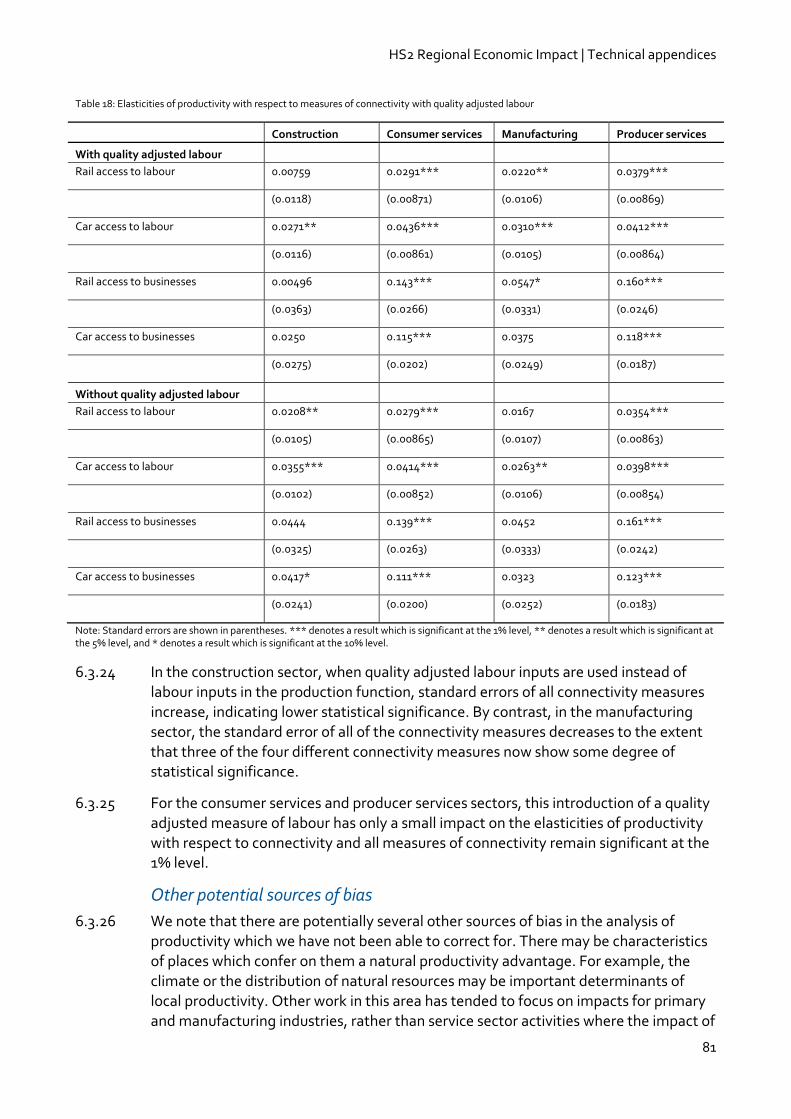
HS2 Regional Economic Impact | Technical appendices
81
Table 18: Elasticities of productivity with respect to measures of connectivity with quality adjusted labour
Construction Consumer services Manufacturing Producer services
With quality adjusted labour
Rail access to labour 0.00759 0.0291*** 0.0220** 0.0379***
(0.0118) (0.00871) (0.0106) (0.00869)
Car access to labour 0.0271** 0.0436*** 0.0310*** 0.0412***
(0.0116) (0.00861) (0.0105) (0.00864)
Rail access to businesses 0.00496 0.143*** 0.0547* 0.160***
(0.0363) (0.0266) (0.0331) (0.0246)
Car access to businesses 0.0250 0.115*** 0.0375 0.118***
(0.0275) (0.0202) (0.0249) (0.0187)
Without quality adjusted labour
Rail access to labour 0.0208** 0.0279*** 0.0167 0.0354***
(0.0105) (0.00865) (0.0107) (0.00863)
Car access to labour 0.0355*** 0.0414*** 0.0263** 0.0398***
(0.0102) (0.00852) (0.0106) (0.00854)
Rail access to businesses 0.0444 0.139*** 0.0452 0.161***
(0.0325) (0.0263) (0.0333) (0.0242)
Car access to businesses 0.0417* 0.111*** 0.0323 0.123***
(0.0241) (0.0200) (0.0252) (0.0183)
Note: Standard errors are shown in parentheses. *** denotes a result which is significant at the 1% level, ** denotes a result which is significant at the 5% level, and * denotes a result which is significant at the 10% level.
6.3.24 In the construction sector, when quality adjusted labour inputs are used instead of labour inputs in the production function, standard errors of all connectivity measures increase, indicating lower statistical significance. By contrast, in the manufacturing sector, the standard error of all of the connectivity measures decreases to the extent that three of the four different connectivity measures now show some degree of statistical significance.
6.3.25 For the consumer services and producer services sectors, this introduction of a quality adjusted measure of labour has only a small impact on the elasticities of productivity with respect to connectivity and all measures of connectivity remain significant at the 1% level.
Other potential sources of bias
6.3.26 We note that there are potentially several other sources of bias in the analysis of productivity which we have not been able to correct for. There may be characteristics of places which confer on them a natural productivity advantage. For example, the climate or the distribution of natural resources may be important determinants of local productivity. Other work in this area has tended to focus on impacts for primary and manufacturing industries, rather than service sector activities where the impact of
HS2 Regional Economic Impact | Technical appendices
82
these factors is likely to be less significant. Other unobserved factors may exist which
could bias the statistical analysis. One approach would be to introduce additional variables into the statistical analysis, such as:
fixed effects for different typologies of area (such as urban, sub-urban, rural);
variables reflecting the quality of the built environment; or
historic levels of public investment.
6.3.27 However, each of these poses challenges of definition and data availability which it has not been possible to investigate further within the limits of this study.
Deriving model parameters
6.3.28 The statistical analysis has shed some light on the importance of connectivity in
driving productivity. However, several features of the data pose significant challenges for using this analysis to model the economic impacts of investment in HS2. In particular, due to the correlation between the connectivity measures, it is not possible to directly estimate their relative importance using a purely statistical approach.
6.3.29 It is clear that the strongest relationships are obtained from the consumer and producer services sectors. This is reassuring because we would expect the performance of these sectors to be more influenced by personal travel rather than the movement of heavy goods. It also appears that, in these two business sectors, the importance of access to businesses consistently produces higher elasticity values than measures of access to labour. We would expect both to be important in determining productivity, but due to the correlation between the different measures we do not have a statistical basis for weighting their relative importance.
6.3.30 A similar issue arises with regard to the importance of the two different modes of transport considered. Across all sectors, the elasticities derived for access to labour by car are higher than those for access by rail, and the statistical significance of the car
labour market measures is higher. For access to businesses, the situation appears to be reversed. In consumer and producer services where the results are consistently statistically significant, the elasticities for rail access to other businesses are higher than those found for access to other businesses by car. In the construction and manufacturing sectors, the elasticities are also higher, although they are not always statistically significant.
6.3.31 Owing to the correlation between the different measures of connectivity, we cannot be certain which is responsible for driving changes in productivity. We therefore need to develop a practical approach that:
captures the best estimate of the overall responsiveness of productivity to changes in connectivity;
represents the effects of labour and business-to-business markets and to the different modes of transport; and
reflects a reasonable view of the relative importance of different types of connectivity to productivity.
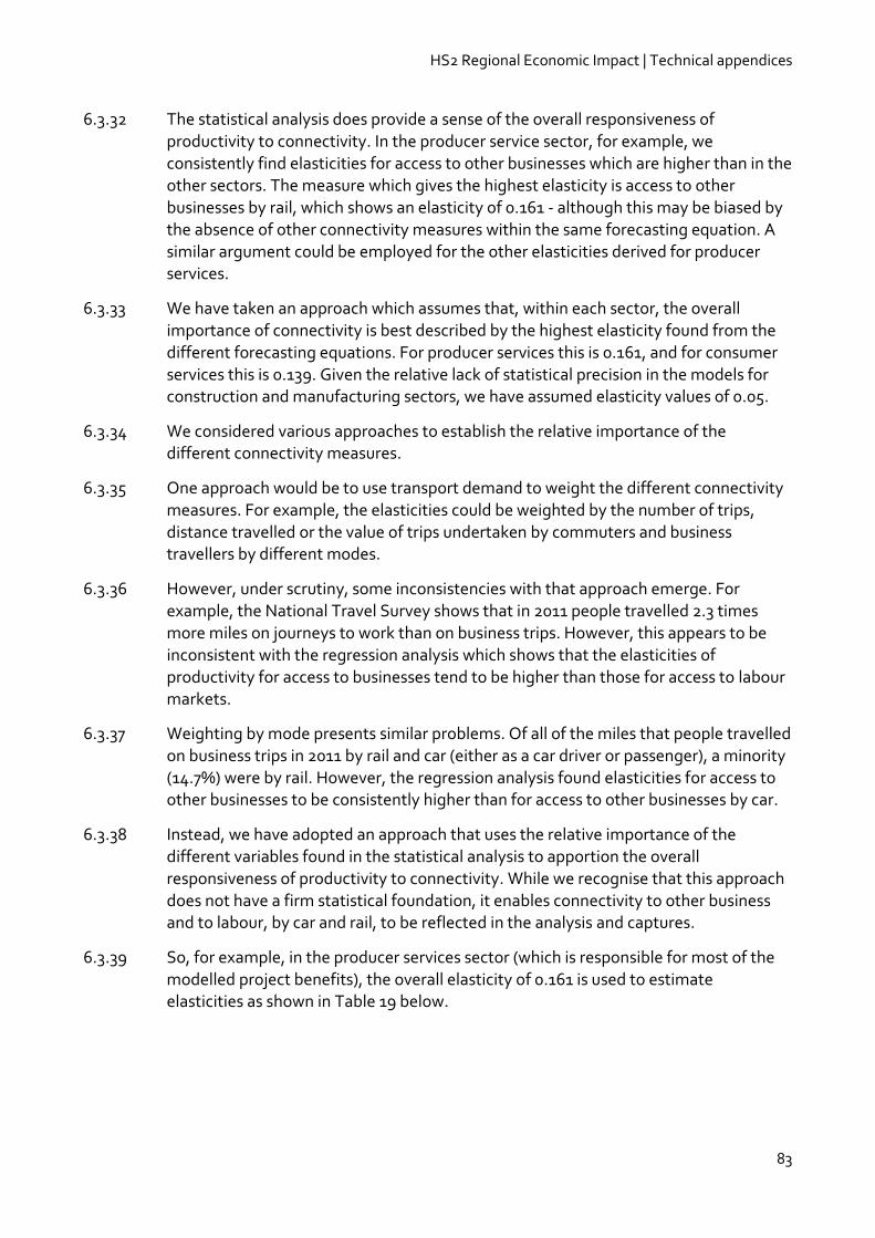
HS2 Regional Economic Impact | Technical appendices
83
6.3.32 The statistical analysis does provide a sense of the overall responsiveness of
productivity to connectivity. In the producer service sector, for example, we consistently find elasticities for access to other businesses which are higher than in the other sectors. The measure which gives the highest elasticity is access to other businesses by rail, which shows an elasticity of 0.161 - although this may be biased by the absence of other connectivity measures within the same forecasting equation. A similar argument could be employed for the other elasticities derived for producer services.
6.3.33 We have taken an approach which assumes that, within each sector, the overall importance of connectivity is best described by the highest elasticity found from the different forecasting equations. For producer services this is 0.161, and for consumer services this is 0.139. Given the relative lack of statistical precision in the models for construction and manufacturing sectors, we have assumed elasticity values of 0.05.
6.3.34 We considered various approaches to establish the relative importance of the different connectivity measures.
6.3.35 One approach would be to use transport demand to weight the different connectivity measures. For example, the elasticities could be weighted by the number of trips, distance travelled or the value of trips undertaken by commuters and business travellers by different modes.
6.3.36 However, under scrutiny, some inconsistencies with that approach emerge. For example, the National Travel Survey shows that in 2011 people travelled 2.3 times more miles on journeys to work than on business trips. However, this appears to be inconsistent with the regression analysis which shows that the elasticities of productivity for access to businesses tend to be higher than those for access to labour markets.
6.3.37 Weighting by mode presents similar problems. Of all of the miles that people travelled on business trips in 2011 by rail and car (either as a car driver or passenger), a minority (14.7%) were by rail. However, the regression analysis found elasticities for access to other businesses to be consistently higher than for access to other businesses by car.
6.3.38 Instead, we have adopted an approach that uses the relative importance of the different variables found in the statistical analysis to apportion the overall responsiveness of productivity to connectivity. While we recognise that this approach does not have a firm statistical foundation, it enables connectivity to other business and to labour, by car and rail, to be reflected in the analysis and captures.
6.3.39 So, for example, in the producer services sector (which is responsible for most of the
modelled project benefits), the overall elasticity of 0.161 is used to estimate elasticities as shown in Table 19 below.
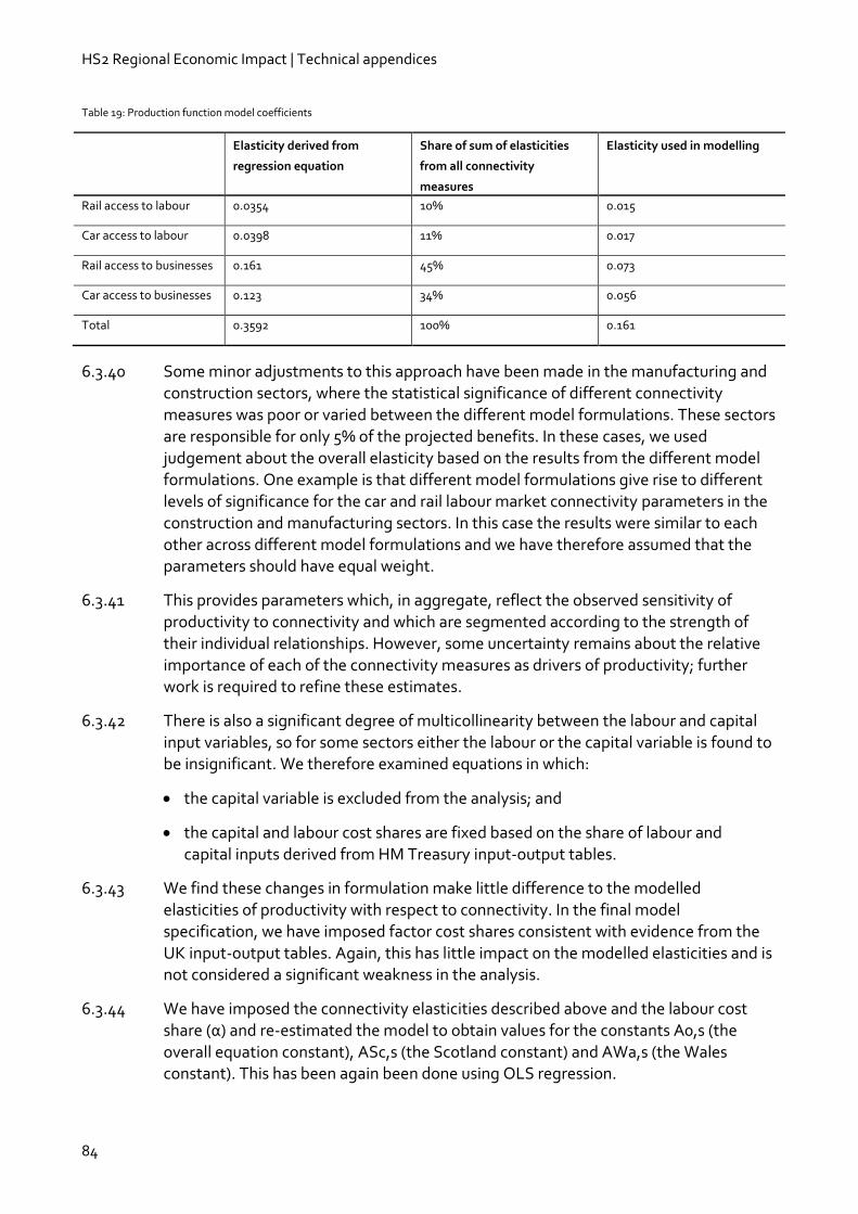
HS2 Regional Economic Impact | Technical appendices
84
Table 19: Production function model coefficients
Elasticity derived from
regression equation
Share of sum of elasticities
from all connectivity
measures
Elasticity used in modelling
Rail access to labour 0.0354 10% 0.015
Car access to labour 0.0398 11% 0.017
Rail access to businesses 0.161 45% 0.073
Car access to businesses 0.123 34% 0.056
Total 0.3592 100% 0.161
6.3.40 Some minor adjustments to this approach have been made in the manufacturing and construction sectors, where the statistical significance of different connectivity
measures was poor or varied between the different model formulations. These sectors are responsible for only 5% of the projected benefits. In these cases, we used judgement about the overall elasticity based on the results from the different model formulations. One example is that different model formulations give rise to different levels of significance for the car and rail labour market connectivity parameters in the construction and manufacturing sectors. In this case the results were similar to each other across different model formulations and we have therefore assumed that the parameters should have equal weight.
6.3.41 This provides parameters which, in aggregate, reflect the observed sensitivity of productivity to connectivity and which are segmented according to the strength of their individual relationships. However, some uncertainty remains about the relative importance of each of the connectivity measures as drivers of productivity; further work is required to refine these estimates.
6.3.42 There is also a significant degree of multicollinearity between the labour and capital input variables, so for some sectors either the labour or the capital variable is found to be insignificant. We therefore examined equations in which:
the capital variable is excluded from the analysis; and
the capital and labour cost shares are fixed based on the share of labour and capital inputs derived from HM Treasury input-output tables.
6.3.43 We find these changes in formulation make little difference to the modelled elasticities of productivity with respect to connectivity. In the final model specification, we have imposed factor cost shares consistent with evidence from the
UK input-output tables. Again, this has little impact on the modelled elasticities and is not considered a significant weakness in the analysis.
6.3.44 We have imposed the connectivity elasticities described above and the labour cost share (α) and re-estimated the model to obtain values for the constants A0,s (the overall equation constant), ASc,s (the Scotland constant) and AWa,s (the Wales constant). This has been again been done using OLS regression.
HS2 Regional Economic Impact | Technical appendices
85
6.3.45 The final model parameters are shown in Table 20 below.
Table 20: Production function model coefficients
Construction Consumer services Manufacturing Producer services
Rail access to labour 0.010 0.016 0.007 0.015
Car access to labour 0.010 0.016 0.010 0.017
Rail access to businesses - 0.060 0.019 0.073
Car access to businesses 0.025 0.048 0.014 0.056
Labour input 0.271 0.410 0.269 0.380
Capital input 0.729 0.590 0.731 0.620
Scotland fixed effect 0.397 0.180 0.292 0.471
Wales fixed effect 0.030 0.001 -0.088 0.145
Constant -0.403 0.803 0.055 0.087
Observations 234 234 234 234
6.3.46 Although not directly comparable, broadly speaking the modelled elasticities are somewhat higher than those used in current transport appraisal guidance which are based on elasticities derived by Imperial College London based on distance based measures of connectivity. However, they are consistent with other work on agglomeration which finds a range from 0.01 to 0.20 described in the Imperial College work.
6.3.47 These parameters are used to model future changes in productivity brought about by
investment in HS2. Estimates of local GDP by business sector are available from the DfT’s Wider Impacts dataset for forecast year 2037. Using the parameters above, we have modelled changes in output by business sector in 2037 as a result of investment in HS2.
Sensitivity testing: mode share based estimates
6.3.48 To reflect the remaining uncertainty about which connectivity variables are driving productivity, we have examined a sensitivity test. This uses estimates of mode share to allocate elasticities rather that the findings from the regression equations. To do this, we have sourced data from the National Travel Survey 2012 which reports the number of miles travelled by car and rail on business trips in 2011. In total rail accounted for 14.7% of all miles travelled on business trips by rail and car in 2011.
6.3.49 No data was available to us to directly capture how mode share varies by business sector. However, the input output tables do show the relative value of rail services and for other land transport services which are purchased by these sectors. For each of the four sectors in our analysis, we have calculated how much of input costs are spent on rail services and on other land transport services. This is around 1.7% of all intermediate consumption costs. Note that the transport, wholesale and warehousing sectors usually included in the consumer services sector, but have been excluded from
HS2 Regional Economic Impact | Technical appendices
86
it for this analysis because of the very high levels of expenditure on the transport sector which predominantly reflects freight activity.
6.3.50 We have then calculated the share of these transport costs which are rail costs and which are other land transport costs. Rail accounts for only around 4.3% of these costs because it has been impossible to separately identify road freight and deliveries which tend to be by road. Across all sectors, we have assumed that this 4.3% share of costs attributable to rail services is consistent with a rail share of business miles travelled of 14.7%.
6.3.51 For each sector, we then factor the rail mode share up or down according to rail’s share of transport costs within that sector. Thus, the consumer services sector (excluding transport and wholesale) has a rail cost share of only 2.0%, which we have taken to imply a rail share of business trip miles of 7.0% (14.7% X 2.0%/4.3%).
However, in the producer services sector, rail’s share of costs is 2.3 times more than all of the sectors averaged together. This implies a rail mode share of 33.5%.
6.3.52 Demand weighting has been applied to the business trip elasticities; however, we
remain unconvinced that distance travelled or trips is a useful way of representing the relative importance of access to labour and access to other businesses. In the sensitivity analysis, we have therefore excluded labour market connectivity from the analysis.
6.3.53 The mode shares have therefore been used to apportion the total elasticity between connectivity to other businesses by rail and connectivity to other businesses by car.
Business location model
6.3.54 Investment in HS2 alters the productivity advantages of different locations. The aim
of the trade model is to estimate how these changes, coupled with the reductions in transport costs of delivering goods and services to different markets, affects the relative competitive position of businesses in different geographical areas.
6.3.55 The business location model hypothesises that the competitive position of location i, when selling goods or services to location j, is a function of the ‘domestic’ productivity in areas i and the transport costs between i and j. It is helpful to consider a number of producing areas (‘i’s) and a number of consuming areas (‘j’s). In fact, we consider that all 235 zones in the PLD model are both producing and consuming areas.
( )
6.3.56 This competitive position of producing location i determines the market share for services in location j that are supplied from location i. We have modelled the
consumption decisions of each location (j) across different potential supplying locations (‘i’s) using a logit choice model. Within this framework, the market share of producer i in market j is determined by the ratio of its competitive position value compared to the sum of all of the competitive position measures from all competing producing areas (‘j’s).
6.3.57 In more formal terms, the market share of location i in market j for product s is given by:
HS2 Regional Economic Impact | Technical appendices
87
( ((
) ))
∑
( ((
) ))
where
Logit scale parameter for sector s
Total production costs of product s in location i
Output in sector s in location i
Number of car business trips per unit of output in sector s
Number of rail business trips per unit of output in sector s
[ ] Generalised cost of travel by mode per unit of output in sector s
6.3.58 The numerator of the above equation is the measure of the competitive position of area i for the market in area j of product s.
6.3.59 The logit scale parameter ( ) is a measure of how much markets are driven to select the most competitive products and hence a measure of their propensity to switch supplier if the cost advantages change. If is small, markets will tend to spread their purchases more evenly across locations with different cost advantages; whereas if is large, consumption will strongly favour the most efficient markets.
6.3.60
reflects the unit costs of ‘domestic’ production in areas i. It is calculated from the
production function analysis which provides units of output in each zone and the total
costs of production which can be calculated from the labour, capital and wage inputs and from the cost of capital. More efficient producing areas (with lower unit costs of production) will be more competitive than other areas.
6.3.61 The next terms in the numerator are the transport cost parameters. These are derived from the observed share of transport costs in different industries drawn from the UK input-output tables 2010 for road transport and rail transport. More information on how these parameters have been derived is provided below. These combine with the unit costs of domestic production to create an overall measure of the cost of producing a unit of output in area i and selling it in area j.
6.3.62 The denominator of the equation is simply the sum of competitive position scores for all producing areas when selling to zone j.
6.3.63 Application of this approach results in modelling the detailed trade relationships between model zones by business sector. This approach enables changes in transport costs to affect the domestic productivity of a location through the production function, but also enables areas to gain or lose market share when exposed to other competing producers which have different domestic production costs. Thus, a firm in Birmingham may become more productive due to agglomeration and become better connected to potential markets in Leeds. If firms in Birmingham have a stronger domestic cost advantage than firms in Leeds, then they will gain market share of the
HS2 Regional Economic Impact | Technical appendices
88
Leeds market. However, a similar process is operating in reverse, whereby firms in
Leeds may gain productivity advantages and easier access to markets in Birmingham. The overall change in market position will be determined by their relative productivity advantages.
Estimating local consumption patterns
6.3.64 HM Treasury releases annual input-output tables which describe the inputs that different business sectors require to create a unit of output, as well as describing household demand for products and services. We have used the input-output tables to calculate intermediate demand (by businesses) and final demand (by households) by sector for the 235 PLD transport model zones. The input assumptions come from two separate tables at a national level for 2010 (which is included in the 2012 edition of the input output tables). All data in the input-output table are presented for 2007 Standard Industrial Classifications (SIC07).
6.3.65 The demand for intermediate inputs in each location is based on the assumed output of these locations. This is constructed from GDP per worker and employment data contained in the DfT’s Wider Impacts Dataset. ‘Local GDP per Worker’ describes the labour productivity of the average worker in each DfT industry in each pre-2009 local authority district. This data has been compiled by DfT using Experian sector productivity forecasts and ONS national GDP forecasts. ‘Local GDP per Worker’ was multiplied by ‘Employment by Sector’ in order to derive a total local GDP estimate for each sector, which was used as an estimate of production output for each sector by local authority district.
6.3.66 HM Treasury input-output tables describe, at a national level, production and consumption by sector in 2010, specified at two-digit SIC07 level of goods produced
and consumed. The intermediate consumption data by two-digit SIC 2007-level sectors was aggregated to DfT’s four sectors. These consumption figures were then split into local authority districts. Given data constraints, the best practice approach to this was considered to be to share national consumption by the share of GDP in each district. This calculation was as follows:
6.3.67 Where s1 = consuming industry; s2 = producing industry; i = local authority; and non-i values refer to national figures.
6.3.68 The above exercise was repeated for final consumption (also sourced from the input-
output tables) to aggregate household expenditure data by two-digit SIC 2007-level sector to DfT’s four sectors. The output of these exercises is total intermediate consumption for each sector of each DfT sector’s goods and services plus the total final consumption of each DfT sector’s goods and services by UK households.
6.3.69 To split final consumption by local authority district, the share of total workplace-based earnings by local authority district was used as a proxy for the total income of the employed population in each district. This is not equivalent to the total income for
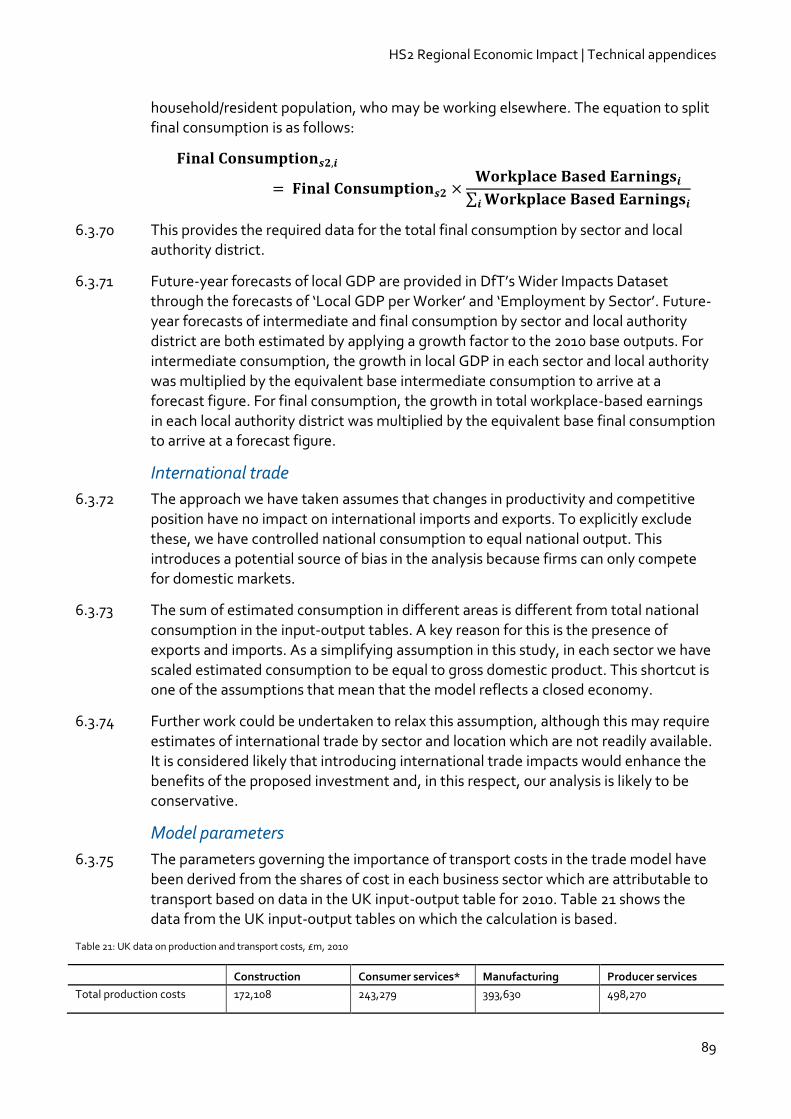
HS2 Regional Economic Impact | Technical appendices
89
household/resident population, who may be working elsewhere. The equation to split final consumption is as follows:
∑
6.3.70 This provides the required data for the total final consumption by sector and local authority district.
6.3.71 Future-year forecasts of local GDP are provided in DfT’s Wider Impacts Dataset through the forecasts of ‘Local GDP per Worker’ and ‘Employment by Sector’. Future-year forecasts of intermediate and final consumption by sector and local authority district are both estimated by applying a growth factor to the 2010 base outputs. For intermediate consumption, the growth in local GDP in each sector and local authority
was multiplied by the equivalent base intermediate consumption to arrive at a forecast figure. For final consumption, the growth in total workplace-based earnings in each local authority district was multiplied by the equivalent base final consumption to arrive at a forecast figure.
International trade
6.3.72 The approach we have taken assumes that changes in productivity and competitive position have no impact on international imports and exports. To explicitly exclude these, we have controlled national consumption to equal national output. This introduces a potential source of bias in the analysis because firms can only compete for domestic markets.
6.3.73 The sum of estimated consumption in different areas is different from total national
consumption in the input-output tables. A key reason for this is the presence of exports and imports. As a simplifying assumption in this study, in each sector we have scaled estimated consumption to be equal to gross domestic product. This shortcut is one of the assumptions that mean that the model reflects a closed economy.
6.3.74 Further work could be undertaken to relax this assumption, although this may require estimates of international trade by sector and location which are not readily available. It is considered likely that introducing international trade impacts would enhance the benefits of the proposed investment and, in this respect, our analysis is likely to be conservative.
Model parameters
6.3.75 The parameters governing the importance of transport costs in the trade model have
been derived from the shares of cost in each business sector which are attributable to transport based on data in the UK input-output table for 2010. Table 21 shows the data from the UK input-output tables on which the calculation is based.
Table 21: UK data on production and transport costs, £m, 2010
Construction Consumer services* Manufacturing Producer services
Total production costs 172,108 243,279 393,630 498,270
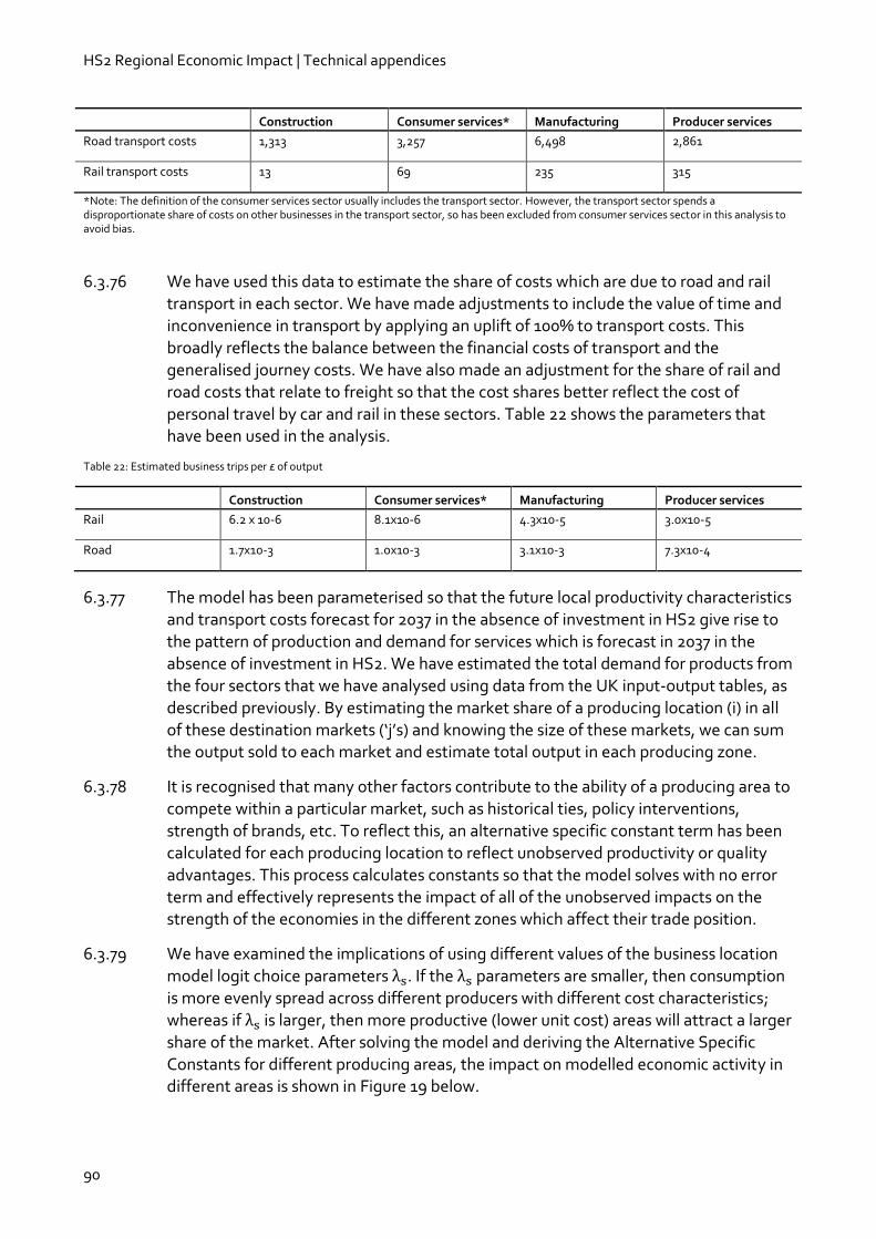
HS2 Regional Economic Impact | Technical appendices
90
Construction Consumer services* Manufacturing Producer services
Road transport costs 1,313 3,257 6,498 2,861
Rail transport costs 13 69 235 315
*Note: The definition of the consumer services sector usually includes the transport sector. However, the transport sector spends a disproportionate share of costs on other businesses in the transport sector, so has been excluded from consumer services sector in this analysis to avoid bias.
6.3.76 We have used this data to estimate the share of costs which are due to road and rail transport in each sector. We have made adjustments to include the value of time and inconvenience in transport by applying an uplift of 100% to transport costs. This broadly reflects the balance between the financial costs of transport and the generalised journey costs. We have also made an adjustment for the share of rail and road costs that relate to freight so that the cost shares better reflect the cost of
personal travel by car and rail in these sectors. Table 22 shows the parameters that have been used in the analysis.
Table 22: Estimated business trips per £ of output
Construction Consumer services* Manufacturing Producer services
Rail 6.2 x 10⁻⁶ 8.1x10⁻⁶ 4.3x10⁻⁵ 3.0x10⁻⁵
Road 1.7x10⁻³ 1.0x10⁻³ 3.1x10⁻³ 7.3x10⁻⁴
6.3.77 The model has been parameterised so that the future local productivity characteristics and transport costs forecast for 2037 in the absence of investment in HS2 give rise to the pattern of production and demand for services which is forecast in 2037 in the absence of investment in HS2. We have estimated the total demand for products from the four sectors that we have analysed using data from the UK input-output tables, as
described previously. By estimating the market share of a producing location (i) in all of these destination markets (‘j’s) and knowing the size of these markets, we can sum the output sold to each market and estimate total output in each producing zone.
6.3.78 It is recognised that many other factors contribute to the ability of a producing area to compete within a particular market, such as historical ties, policy interventions, strength of brands, etc. To reflect this, an alternative specific constant term has been calculated for each producing location to reflect unobserved productivity or quality advantages. This process calculates constants so that the model solves with no error term and effectively represents the impact of all of the unobserved impacts on the strength of the economies in the different zones which affect their trade position.
6.3.79 We have examined the implications of using different values of the business location
model logit choice parameters . If the parameters are smaller, then consumption is more evenly spread across different producers with different cost characteristics; whereas if is larger, then more productive (lower unit cost) areas will attract a larger share of the market. After solving the model and deriving the Alternative Specific Constants for different producing areas, the impact on modelled economic activity in different areas is shown in Figure 19 below.
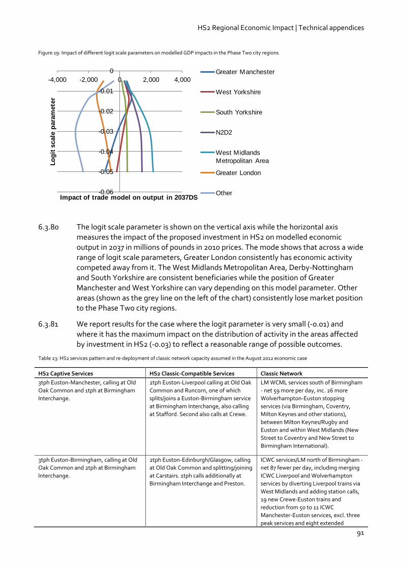
HS2 Regional Economic Impact | Technical appendices
91
Figure 19: Impact of different logit scale parameters on modelled GDP impacts in the Phase Two city regions
6.3.80 The logit scale parameter is shown on the vertical axis while the horizontal axis measures the impact of the proposed investment in HS2 on modelled economic output in 2037 in millions of pounds in 2010 prices. The mode shows that across a wide range of logit scale parameters, Greater London consistently has economic activity competed away from it. The West Midlands Metropolitan Area, Derby-Nottingham and South Yorkshire are consistent beneficiaries while the position of Greater Manchester and West Yorkshire can vary depending on this model parameter. Other areas (shown as the grey line on the left of the chart) consistently lose market position to the Phase Two city regions.
6.3.81 We report results for the case where the logit parameter is very small (-0.01) and where it has the maximum impact on the distribution of activity in the areas affected by investment in HS2 (-0.03) to reflect a reasonable range of possible outcomes.
Table 23: HS2 services pattern and re-deployment of classic network capacity assumed in the August 2012 economic case
HS2 Captive Services HS2 Classic-Compatible Services Classic Network
3tph Euston-Manchester, calling at Old
Oak Common and 1tph at Birmingham
Interchange.
2tph Euston-Liverpool calling at Old Oak
Common and Runcorn, one of which
splits/joins a Euston-Birmingham service
at Birmingham Interchange, also calling
at Stafford. Second also calls at Crewe.
LM WCML services south of Birmingham
- net 59 more per day, inc. 26 more
Wolverhampton-Euston stopping
services (via Birmingham, Coventry,
Milton Keynes and other stations),
between Milton Keynes/Rugby and
Euston and within West Midlands (New
Street to Coventry and New Street to
Birmingham International).
3tph Euston-Birmingham, calling at Old
Oak Common and 2tph at Birmingham
Interchange.
2tph Euston-Edinburgh/Glasgow, calling
at Old Oak Common and splitting/joining
at Carstairs. 1tph calls additionally at
Birmingham Interchange and Preston.
ICWC services/LM north of Birmingham -
net 87 fewer per day, including merging
ICWC Liverpool and Wolverhampton
services by diverting Liverpool trains via
West Midlands and adding station calls,
19 new Crewe-Euston trains and
reduction from 50 to 11 ICWC
Manchester-Euston services, excl. three
peak services and eight extended
-0.06
-0.05
-0.04
-0.03
-0.02
-0.01
0
-4,000 -2,000 0 2,000 4,000
Lo
git
scale
para
mete
r
Impact of trade model on output in 2037DS
Greater Manchester
West Yorkshire
South Yorkshire
N2D2
West Midlands
Metropolitan Area
Greater London
Other

HS2 Regional Economic Impact | Technical appendices
92
HS2 Captive Services HS2 Classic-Compatible Services Classic Network
to/from Edinburgh. (NB overall
Manchester-Euston frequency
increased.)
3tph Euston-Leeds, calling at Old Oak
Common and two at Toton, two at
Sheffield and one at Birmingham
Interchange.
1tph provides second hourly service
to/from Preston, also calling at Old Oak
Common, Crewe, Warrington and
Wigan.
MML/Thameslink via MML - net 4 more
services per day, including new 16-train
Bedford-St Pancras service and a
reduction in longer distance MML
services between Sheffield, Derby and
Nottingham from 60 to 48.
2tph Birmingham-Manchester. 2tph to/from Newcastle, also calling at
Old Oak Common and either York or
Darlington.
ICEC, Great Northern and TransPennine -
net 11 fewer services per day, new 16-
train Peterborough-King’s Cross service,
from 1 to 16 Lincoln-King’s Cross trains,
reduction from 45 to 16 ICEC Leeds-
London services (NB overall Leeds-
Euston frequency increased) and 10
fewer ICEC Edinburgh-London services
(note ICWC services via Manchester
described above).
2tph Birmingham-Leeds, calling at Toton
and Sheffield.
1tph providing a second hourly service
to/from York, also calling at Old Oak
Common and Toton.
CrossCountry services to North East and
North West - no change in frequency,
additional stops at Birmingham
International, Coventry, Sheffield HS,
Toton, Alfreton, Macclesfield and
Congleton, and some services shortened
from Edinburgh/Newcastle to
Newcastle/York.
1tph Heathrow-Manchester, calling at
Birmingham Interchange.
1tph Birmingham-Edinburgh or Glasgow
(in alternate hours), calling at Wigan,
Preston, Carlisle and Lockerbie, plus
either Lancaster and Penrith, or
Oxenholme.
East Midlands local services - no
frequency changes, additional stops at
Toton, some services to/from
Nottingham extended to/from Leicester.
1tph Heathrow-Leeds, calling at
Birmingham Interchange, Toton and
Sheffield
1tph Birmingham-Newcastle, calling at
Toton, Sheffield, York, Darlington and
Durham.
Northern England local services - 64 new
semi-fast local services per day including
32 Leeds-Doncaster trains, 16
Manchester-Crewe services and 16
Manchester-Stoke trains.