A&A 641, A146 (2020)https://doi.org/10.1051/0004-6361/202038732c© ESO 2020

Astronomy&Astrophysics

High-resolution observations of the solar photosphere,chromosphere, and transition region

A database of coordinated IRIS and SST observations

L. H. M. Rouppe van der Voort1,2, B. De Pontieu3,1,2, M. Carlsson1,2, J. de la Cruz Rodríguez4, S. Bose1,2,G. Chintzoglou3,5, A. Drews1,2, C. Froment1,2,6, M. Gošic3,7, D. R. Graham3,7, V. H. Hansteen1,2,3,7,

V. M. J. Henriques1,2, S. Jafarzadeh1,2, J. Joshi1,2, L. Kleint8,9, P. Kohutova1,2, T. Leifsen1,2,J. Martínez-Sykora3,7,1,2, D. Nóbrega-Siverio1,2, A. Ortiz1,2, T. M. D. Pereira1,2, A. Popovas1,2, C. Quintero Noda1,2,A. Sainz Dalda3,7,10, G. B. Scharmer4, D. Schmit11,12, E. Scullion13,1, H. Skogsrud1, M. Szydlarski1,2, R. Timmons3,

G. J. M. Vissers4,1, M. M. Woods3,6, and P. Zacharias1

1 Institute of Theoretical Astrophysics, University of Oslo, PO Box 1029, Blindern 0315, Oslo, Norwaye-mail: rouppe@astro.uio.no

2 Rosseland Centre for Solar Physics, University of Oslo, PO Box 1029, Blindern 0315, Oslo, Norway3 Lockheed Martin Solar & Astrophysics Laboratory, 3251 Hanover St., Palo Alto, CA 94304, USA4 Institute for Solar Physics, Dept. of Astronomy, Stockholm University, AlbaNova University Centre, 10691 Stockholm, Sweden5 University Corporation for Atmospheric Research, Boulder, CO 80307-3000, USA6 LPC2E, CNRS and University of Orléans, 3A avenue de la Recherche Scientifique, Orléans, France7 Bay Area Environmental Research Institute, NASA Research Park, Moffett Field, CA 94035, USA8 University of Applied Sciences and Arts Northwestern Switzerland, Bahnhofstrasse 6, 5210 Windisch, Switzerland9 Leibniz-Institut für Sonnenphysik (KIS), Schöneckstrasse 6, D-79104 Freiburg, Germany

10 Stanford University, HEPL, 466 Via Ortega, Stanford, CA 94305-4085, USA11 Catholic University of America, Washington, DC 20064, USA12 NASA Goddard Space Flight Center, Greenbelt, MD 20771, USA13 Department of Mathematics, Physics and Electrical Engineering, Northumbria University, Newcastle upon Tyne NE1 8ST, UK

Received 24 June 2020 / Accepted 21 July 2020

ABSTRACT

NASA’s Interface Region Imaging Spectrograph (IRIS) provides high-resolution observations of the solar atmosphere through ultra-violet spectroscopy and imaging. Since the launch of IRIS in June 2013, we have conducted systematic observation campaigns incoordination with the Swedish 1 m Solar Telescope (SST) on La Palma. The SST provides complementary high-resolution observa-tions of the photosphere and chromosphere. The SST observations include spectropolarimetric imaging in photospheric Fe i lines andspectrally resolved imaging in the chromospheric Ca ii 8542 Å, Hα, and Ca ii K lines. We present a database of co-aligned IRIS andSST datasets that is open for analysis to the scientific community. The database covers a variety of targets including active regions,sunspots, plages, the quiet Sun, and coronal holes.

Key words. Sun: photosphere – Sun: chromosphere – Sun: transition region – sunspots – Sun: faculae, plages

1. Introduction

The solar atmosphere is a very dynamic region, where funda-mental physical processes take place on small spatial scales andshort dynamical time scales, often leading to rapid changes inthe thermodynamic state of the plasma. Resolving these pro-cesses in observations requires high resolution in the combinedspatial, temporal, and spectral domains. Furthermore, the com-bination of multiple spectral diagnostics, preferably with sen-sitivity to line formation conditions that cover a large rangein temperatures, densities, and magnetic field topologies, areof fundamental importance for advancing our understanding ofthe solar atmosphere. The simultaneous acquisition of vastlydifferent spectral diagnostics is possible through coordinatedobservations between space-borne and ground-based observingfacilities. Telescopes in space provide unique access to the short

wavelength regime with seeing-free diagnostics of the chromo-sphere, transition region and corona. Ground-based telescopesallow for high resolution in photospheric and chromosphericdiagnostics, as well as high-sensitivity polarimetric measure-ments of the magnetic field with instrumentation that can bemore complex than in space, and which is not limited bydata transfer rates. Coordinated observations, therefore, stronglyenhance the potential to unravel connections in the solar atmo-sphere that span from the photosphere, through the chromo-sphere and transition region to the corona.

The Interface Region Imaging Spectrograph (IRIS, DePontieu et al. 2014a), a NASA Small Explorer (SMEX)satellite, was launched on 2013-Jun-27. It combines high res-olution in the spatial (0′′.3–0′′.4), temporal (down to 1 s), andspectral domains (velocity determination down to 1 km s−1).Spectral diagnostics include the Mg ii h & k resonance lines

Article published by EDP Sciences A146, page 1 of 9

A&A 641, A146 (2020)

(chromosphere), the C ii lines at 1335 Å (upper chromosphereand transition region), and the Si iv lines at 1400 Å (transitionregion). Furthermore, the (weaker) O iv lines around 1400 Å aswell as the Fexii 1349 Å and Fexxi 1354 Å lines provide diag-nostics on the corona and high-energy flares. Slit-jaw imagingin the Mg ii k core, Mg ii h wing, C ii, and Si iv lines providesvaluable context information.

The IRIS satellite offers considerable flexibility in its observ-ing configuration, and, for example, allows for a wide variety inarea coverage (i.e., field-of-view (FOV) size), temporal cadence,and choice of spectral diagnostics. Target selection is organizedthrough a system with relatively short communication lines andallows for effective coordination with ground-based telescopesand other observing facilities. This has opened up possibilities toexpand on IRIS’s rich arsenal of spectral diagnostics, for exam-ple by adding photospheric and chromospheric spectropolarime-try and high-resolution imaging in various spectral lines at andaround the area covered by the IRIS spectrograph slit.

Shortly after IRIS was launched, scientists from the Univer-sity of Oslo and from the Lockheed Martin Solar and Astro-physics Laboratory (LMSAL) started organizing coordinatedobserving campaigns with the Swedish 1-m Solar Telescope(SST, Scharmer et al. 2003a) on La Palma. Every year, four cam-paigns – typically two weeks each – are conducted during theSST observing season (April – October). The SST is capable ofproviding high-quality time series of spectrally resolved photo-spheric and chromospheric diagnostics that under excellent see-ing conditions reach the diffraction limit of <0′′.1 over the fullarcmin2 FOV. Furthermore, the versatile CRISP instrument canprovide spectropolarimetric data that enable the measurement ofthe magnetic field topology. In addition, the tunable filter sys-tem CHROMIS, installed in 2016, can simultaneously providenarrowband filtergrams at several wavelengths in the core of theCa ii K line.

Data from the coordinated campaigns have been used to studya variety of topics, including: the disk counterparts of spicules(De Pontieu et al. 2014b; Rouppe van der Voort et al. 2015;Rutten & Rouppe van der Voort 2017; Martínez-Sykora et al.2017; Bose et al. 2019a), chromospheric bright grains in the inter-network (Martínez-Sykora et al. 2015) and active region plage(Skogsrud et al. 2016), penumbral microjets in sunspots (Visserset al. 2015a; Drews & Rouppe van der Voort 2020), the atmo-spheric stratification in plage (Carlsson et al. 2015) and sunspots(Bose et al. 2019b), the relation between Ellerman Bombs andultraviolet (UV) bursts (Vissers et al. 2015b; Hansteen et al. 2017;Rouppe van der Voort et al. 2017; Vissers et al. 2019; Ortiz et al.2020), Ellerman bombs in the quiet Sun (Rouppe van der Voortet al. 2016), magnetic flux emergence from the photosphere to thetransition region (Ortiz et al. 2016), surges (Nóbrega-Siverio et al.2017), and the chromospheric counterparts of transition-regionunresolved fine structure loops (Pereira et al. 2018).

In this paper, we describe the public release of co-alignedIRIS and SST data. At first, the public release is limited to dataproducts that share the same plate scale as IRIS (0′′.17 per pixel)for easier data analysis. This pixel scale implies that the spatialresolution of the SST data is degraded. The release of the cor-responding full spatial resolution SST data is planned for futuredata releases.

2. Observations and data processing

2.1. IRIS

The IRIS telescope design and instrumentation are described inDe Pontieu et al. (2014a). The IRIS satellite acquires spectra

in three spectral regions: in the far UV from 1332 to 1358 Å(FUV1), in the far UV from 1389 to 1407 Å (FUV2), and in thenear UV from 2783 to 2834 Å (NUV). The FUV1 region is dom-inated by the C ii lines at 1334 and 1335 Å that are formed in theupper chromosphere (Rathore et al. 2015a,b), the FUV2 region isdominated by the Si iv lines at 1394 and 1403 Å that are formedin the transition region. The NUV region is dominated by thechromospheric Mg ii h and k lines (Leenaarts et al. 2013a,b), andfurther hosts the upper photospheric and lower chromosphericMg ii triplet lines (Pereira et al. 2015) and a large number of(upper) photospheric blends in the strong Mg ii wings (Pereiraet al. 2013).

The 0′′.33 wide spectrograph slit has a length of 175′′ andcan be displaced with respect to the solar surface to build up araster that samples an area up to 130′′ × 175′′. There are severalchoices of step sizes between consecutive slit positions: densesampling with 0′′.35 steps, sparse sampling with 1′′ steps, orcoarse sampling with 2′′ steps. Alternatively, the spectrographcan record data in a sit-and-stare mode, where the slit does notmove and stays at a fixed location (with or without tracking forsolar rotation).

The IRIS satellite can take slit-jaw images (SJIs) with dif-ferent filters to provide context around the spectrograph slit. Thefour science SJI channels are: SJI 2796, centered on Mg ii k (4 Åbandpass); SJI 2832, centered at 2830 Å in the Mg ii h wing (4 Åbandpass); SJI 1330, centered at 1340 Å and dominated by theC ii lines (55 Å bandpass); and SJI 1400, centered at 1390 Å anddominated by the Si iv lines (55 Å bandpass). Slit-jaw imagesfrom different channels are recorded sequentially and have thesame exposure time as the spectrograms recorded with the spec-trograph.

Various choices can be made to reduce the data volume inorder to fit within the daily limits of data transfer from the space-craft to ground stations. For each spectral line of interest, thewavelength range can be selected to limit the data transferred,or the spatial extent of the raster can be limited by transferringonly data from a reduced part along the slit. Other measuresto reduce data transfer are compression, data binning (spatiallyand/or spectrally), and omitting one or several SJI channels(most frequently SJI 2832 is omitted, although this is often doneto improve the cadence of the other SJI channels).

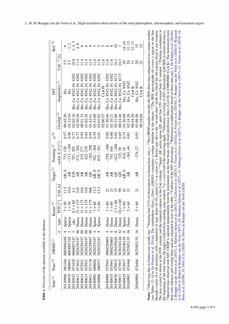
Taken together, the various possible choices in raster stepsize, number of slit positions, slit length, SJI channel selection,exposure time, spatial and spectral binning, compression, andspectral line selection (line lists) constitute a considerable num-ber of possible observing programs. These programs are identi-fied by a unique number, the OBS number (or OBSID; for moredetails, see De Pontieu et al. 2014a). The OBSID, together withthe observing date and start time, constitute a unique identifierfor each dataset (see the first three columns in Table 1).

2.2. SST

The SST telescope design and its main optical elements aredescribed in Scharmer et al. (2003a). A description of upgradesof optical components and instrumentation, as well as a thor-ough evaluation of optical performance is provided by Scharmeret al. (2019). An adaptive optics system is fully integrated inthe optical system (Scharmer et al. 2003b) and was upgradedwith an 85-electrode deformable mirror operating at 2 kHz in2013. A dichroic beam splitter divides the beam on the opti-cal table into a red (>500 nm) and a blue beam. Both beamsare equipped with tunable filter instruments: the CRISP imaging

A146, page 2 of 9

L. H. M. Rouppe van der Voort et al.: High-resolution observations of the solar photosphere, chromosphere, and transition region

Tabl

e1.

Ove

rvie

wof

the

data

sets

avai

labl

ein

the

data

base

.

Dat

e(a

)Ti

me

(b)

OB

SID

(c)

Ras

ter(d

)Ta

rget

(e)

Poin

ting

(f)

µ(g

)SS

TR

ef.(k

)

nty

peFO

V[′′

]C

ad.[

s](s

olar

X,Y

)[′′

]O

verl

ap(h

)di

agno

stic

s(i

)C

ad.(j

)[s

]

2013

0906

0811

0440

0300

4168

4Sp

arse

3×

5011

.5A

R,S

773,

128

0.57

00:4

5:30

Hα

5.5

620

1309

1008

0943

4003

0071

652

Spar

se1×

5010

.0A

R−

173,−

189

0.96

01:1

2:54

Hα

5.5

1,2

2013

0922

0734

3040

0400

7147

1s&

s0.

3×

604.

2C

H55

1,29

50.

7702

:02:

16Hα

,Ca

8542

,Fe

6302

10.9

1,2,

320

1406

1107

3631

3820

2561

9796

Den

se31×

175

516

AR

573,−

202

0.77

02:5

0:38

Hα

,Ca

8542

,Fe

6302

11.4

4,8

2014

0614

0729

3138

2025

6197

96D

ense

31×

175

516

AR

235,

277

0.92

00:5

1:32

Hα

,Ca

8542

,Fe

6302

11.4

620

1406

1507

2931

3820

2561

9796

Den

se31×

175

516

AR

425,

278

0.84

01:0

2:36

Hα

,Ca

8542

,Fe

6302

11.4

620

1406

2107

3138

3820

2594

9796

Den

se31×

175

908

QS

−20

1,25

80.

9401

:43:

41Hα

,Ca

8542

,Fe

6302

11.5

920

1409

0508

0604

3820

2551

674

Spar

se3×

6013

.2A

R,S

702,−

304

0.59

01:5

3:00

Hα

,Ca

8542

,Fe

6302

11.6

520

1409

0608

0537

3820

2551

674

Spar

se3×

6013

.2A

R,S

819,−

281

0.41

02:0

1:02

Hα

,Ca

8542

,Fe

6302

11.6

502

:00:

53C

aii

H11

.65

2014

0909

0759

4338

6025

6865

4D

ense

1×

6021

AR

−23

0,−

366

0.89

01:5

0:46

Hα

,Ca

8542

,Fe

6302

11.6

820

1409

1507

4941

3860

2568

654

Den

se1×

6021

AR

743,

164

0.60

01:1

6:21

Hα

,Ca

8542

,Fe

6302

11.6

820

1506

2607

0915

3630

1054

268

Den

se2.

3×

6025

QS

−42

2,−

260

0.85

02:3

1:06

Hα

,Ca

8542

,Fe

6173

16.1

1020

1509

1707

3915

3630

1041

4432

Den

se10.2×

6099

QS

725,

380.

6500

:24:

46Hα

,Ca

8542

,Fe

6173

24.1

720

1604

2907

4917

3620

1061

298

Spar

se7×

6041

AR

,S63

4,18

0.74

01:3

0:09

Hα

,Ca

8542

2014

,16

2016

0903

0744

4636

2550

3135

16D

ense

5×

6021

AR

−56

1,44

0.81

02:1

4:30

Hα

,Ca

8542

2011

,15

00:3

4:20

Caii

K13

12,1

320

1609

0407

4446

3625

5031

3516

Den

se5×

6021

AR

−37

4,27

0.91

01:0

9:36

Hα

,Ca

8542

2015

00:3

4:04

Caii

K22

12

Not

es.(a

) Obs

ervi

ngda

tein

form

atye

ar,m

onth

,day

.(b) St

artin

gtim

e(U

T)o

fobs

erva

tions

info

rmat

hour

,min

,s.(c

) The

OB

SID

num

bere

ncod

esth

eIR

ISob

serv

ing

confi

gura

tion

ina

uniq

uenu

mbe

r(s

eeTa

bles

12–1

4in

De

Pont

ieu

etal

.201

4a).

The

com

bina

tion〈D

ate〉

_〈Ti

me〉

_〈O

BSI

D〉

cons

titut

esa

uniq

ueid

entifi

erto

the

data

set.

(d) T

heIR

ISsp

ectr

ogra

phsl

itco

vers

are

gion

onth

eSu

nth

roug

ha

rast

erof

nsl

itpo

sitio

ns,w

itha

sepa

ratio

nof

type

:den

se(0′′ .3

5),s

pars

e(1′′

),or

coar

se(2′′

).R

aste

rty

pes&

sis

the

“sit-

and-

star

e”m

ode

for

whi

chth

esl

itre

mai

nsfix

edat

one

loca

tion.

The

area

cove

red

issh

own

inth

eFO

Vco

lum

n,an

dth

ete

mpo

ralc

aden

cein

the

Cad

.col

umn.

(e) Ta

rget

:AR

:act

ive

regi

on,Q

S:qu

ietS

un,C

H:c

oron

alho

le,S

:sun

spot

.(f) Po

intin

gco

ordi

nate

sat

the

begi

nnin

gof

the

time

seri

es,t

heta

rget

isfo

llow

edby

trac

king

sola

rrot

atio

n.(g

) µ=

cosθ

with

θth

eob

serv

ing

angl

e.(h

) Dur

atio

nof

over

lap

ofSS

Tob

serv

atio

nsw

ithIR

ISin

form

athh

:mm

:ss.

(i) Sp

ectr

allin

esob

serv

edw

ithSS

T.C

RIS

Pis

oper

ated

inde

pend

ently

from

the

inst

rum

ents

onth

ebl

uebe

am;w

ithfix

edin

terf

eren

cefil

ters

(Caii

H)o

rCH

RO

MIS

(Caii

K).

The

inst

rum

ents

have

thei

row

nca

denc

esan

dov

erla

ptim

esan

dar

ese

para

ted

inro

ws

inth

eta

ble.

(j) C

aden

ceof

the

SST

obse

rvat

ions

.(k) R

efer

ence

sto

publ

icat

ions

base

don

thes

eda

tase

ts:1

:De

Pont

ieu

etal

.(20

14b)

,2:

Rou

ppe

van

derV

oort

etal

.(20

15),

3:M

artín

ez-S

ykor

aet

al.(

2015

),4:

Car

lsso

net

al.(

2015

)5:V

isse

rset

al.(

2015

a),6

:Vis

sers

etal

.(20

15b)

,7:R

oupp

eva

nde

rVoo

rtet

al.(

2016

)8:S

kogs

rud

etal

.(20

16)

9:R

utte

n&

Rou

ppe

van

der

Voor

t(20

17),

10:M

artín

ez-S

ykor

aet

al.(

2017

),11

:Nób

rega

-Siv

erio

etal

.(20

17),

12:R

oupp

eva

nde

rVo

orte

tal.

(201

7),1

3:V

isse

rset

al.(

2019

),14

:B

ose

etal

.(20

19b)

,15:

Ort

izet

al.(

2020

)16:

Dre

ws

&R

oupp

eva

nde

rVoo

rt(2

020)

.

A146, page 3 of 9

A&A 641, A146 (2020)

spectropolarimeter (Scharmer et al. 2008) on the red beam, andthe CHROMIS imaging spectrometer on the blue beam. BothCRISP and CHROMIS are dual Fabry–Pérot filtergraph systemsbased on the design by Scharmer (2006) and are capable of fastwavelength sampling of spectral lines. Before the installationof CHROMIS in September 2016, the blue beam was equippedwith a number of interference filters, including a full width athalf maximum (FWHM) of 10 Å wide filter for photosphericimaging at 3954 Å, and an FWHM = 1 Å wide filter centeredon the Ca ii H line core at λ = 3968 Å (see Löfdahl et al.2011). The CRISP instrument has a pair of liquid crystals thattogether with a polarising beam splitter allow measurements ofcircular and linear polarisation in for example the photosphericFe i 6173 Å, Fe i 6301 Å, and Fe i 6302 Å lines, and the chromo-spheric Ca ii 8542 Å line.

The CRISP instrument has a plate scale of 0′′.058 per pixeland the SST diffraction limit (λ/D) is 0′′.14 at the wavelengthof Hα (with the telescope aperture diameter D = 0.97 m). Thetransmission profile of CRISP has FWHM = 60 mÅ at thewavelength of Hα. The CHROMIS instrument has a plate scaleof 0′′.038 per pixel and the SST diffraction limit is 0′′.08 at thewavelength of Ca ii K. The transmission profile of CHROMIShas FWHM ≈ 120 mÅ at the wavelength of Ca ii K. The FOVof CRISP and CHROMIS is approximately 1′ × 1′. We note thatsunlight collected by the SST is split by a dichroic beam splittersuch that CRISP and CHROMIS can operate independently andin parallel, without reducing the efficiency of either instrument.

Image restoration by means of the multi-object multi-frameblind deconvolution (MOMFBD, Löfdahl et al. 2002; van Noortet al. 2005) method is applied to all data to enhance imagequality over the full FOV. The MOMFBD restoration is inte-grated in the CRISP and CHROMIS data processing pipelines(de la Cruz Rodríguez et al. 2015; Löfdahl et al. 2018).These pipelines include the method described by Henriques(2012) for consistency between sequentially recorded liquidcrystal states and wavelengths, with destretching performed asin Shine et al. (1994). The CRISP and CHROMIS instrumentsinclude auxiliary wideband (WB) systems which are essentialas anchor channels in MOMFBD restoration. Furthermore, theyprovide photospheric reference channels that facilitate preciseco-alignment between CRISP and CHROMIS data (or blue beamfilter data before 2016), or co-alignment with data from IRIS andthe Solar Dynamic Observatory (SDO, Lemen et al. 2012).

2.3. SST observing programs

The SST observing programs vary from campaign to campaign,and often during campaigns as well, depending on the targetand science goals. Common to all datasets in the database is theinclusion of at least one chromospheric line, Hα or Ca ii 8542 Å,and often both. In order to keep the temporal cadence below 20 s,the Ca ii 8542 Å observations were most often carried out in non-polarimetric mode.

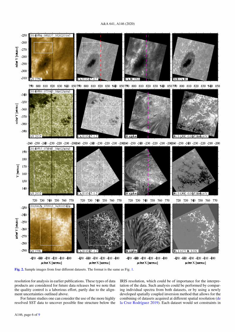
During the 2013 and 2014 observing seasons, photosphericspectropolarimetry was limited to one single position in the bluewing of the Fe i 6302 Å line. The Stokes V maps serve as effec-tive locators of the strongest magnetic field regions and polarityindicators. An example of such a blue wing Fe i 6302 Å Stokes Vmap can be seen in Fig. 2 for the 2014-Sep-09 and 2014-Sep-15datasets, as well as in Fig. 4.

During later campaigns, spectral sampling of photosphericFe i lines was extended. These observations were subjected to afast and robust pixel-to-pixel Milne-Eddington (ME) inversion

procedure. The parallel C++ implementation1 (de la CruzRodríguez 2019) is based upon the analytical intensity deriva-tives described by Orozco Suárez & Del Toro Iniesta (2007) andan efficient Levenberg-Marquardt algorithm that is described inde la Cruz Rodríguez et al. (2019).

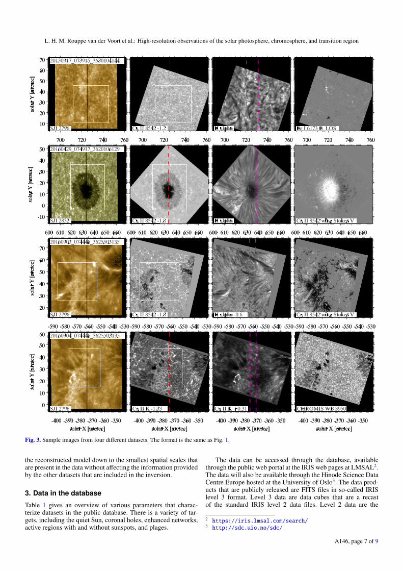
Example line of sight (LOS) magnetic field strength (BLOS)maps from Fe i 6173 Å inversions are shown in Fig. 2 forobserving date 2015-Jun-26 and in Fig. 3 for 2015-Sep-17. Thedatabase contains maps of BLOS, plane of the sky magnetic fieldstrength Bperp, and LOS velocity from these ME inversions.

For datasets for which spectropolarimetric Ca ii 8542 Åobservations were taken, we include magnetograms that wereconstructed by summing Stokes V data from the blue wing ofthe Ca ii line, and subtracting the corresponding sum from thered wing. These serve as photospheric magnetic field maps ina similar way as the Fe i 6302 Å Stokes V maps. Examplescan be found in Fig. 3 for observing dates 2016-Apr-29 and2016-Sep-03.

2.4. IRIS and SST co-alignment

For the co-alignment of the IRIS and SST data, we employ cross-correlation of image pairs that are morphologically as similar aspossible. Most often, the SJI 2796 and Ca ii 8542 Å wing (at0.8–1.2 Å offset from line core) or Ca ii K wing show similarenough scenes to give satisfying results. This is particularlytrue for more quiet regions with the characteristic mesh-likepattern from acoustic shocks and the surrounding network ofhigh-contrast bright regions. For active regions with enhancedflaring activity or large sunspots, the SJI 2796 and Ca ii 8542 Åwing pair can have more dissimilar scenes and therefore theco-alignment can be less reliable.

The combination SJI 2832 with CRISP WB or Hα far winggives excellent co-alignment results since both channels showpure photospheric scenes. However, SJI 2832 is not alwaysselected for the IRIS observing programs to limit the data rateand improve the cadence of the other SJI channels.

Before cross-correlation, the plate scales between imagepairs are matched. Offsets are then determined by cross-correlation over a subfield of the common FOV of image pairsthat are closest in time. Examples of such subfields are out-lined by white rectangles in Figs. 1–4. The raw offsets are thensmoothed with a temporal window to account for jitter due tonoise. The offsets that are applied to the data are interpolated tothe relevant time grid of the particular diagnostic.

The precision of the alignment is limited by a number offactors. Formation height differences between the diagnosticsused for cross-correlation may introduce a systematic offset thatis difficult to account for. This is probably of limited concernfor cross-correlation between photospheric diagnostics involv-ing SJI 2832, but it is more uncertain between SJI 2796 andthe Ca ii 8542 wing. The systematic offset may be higher foroblique observing angles towards the limb and may also dependon the type of target (for example, active regions with flaringactivity that appears less prominent in the Ca ii 8542 wing thanin the Mg ii k core). Furthermore, varying seeing conditions atthe SST inevitably lead to image distortions that cannot be fullyaccounted for in post-processing. We estimate that the error inthe co-alignment can be as good as or better than one IRIS pixel(0′′.17, in the case of SST data taken under excellent conditionsand closely matching diagnostic pairs in the cross-correlation).

1 https://github.com/jaimedelacruz/pyMilne

A146, page 4 of 9

L. H. M. Rouppe van der Voort et al.: High-resolution observations of the solar photosphere, chromosphere, and transition region

Fig. 1. Sample images from four different datasets. Each row shows four different diagnostics. The first two images on each row show the channelpairs that were used for IRIS and SST co-alignment and the area outlined by the white rectangle marks the region used for cross-correlation todetermine offsets. The dashed red line in the second image marks the location of the IRIS slit in the SJI image to the left. The dashed purple linesin the third image mark the area covered by the IRIS raster. The SST images are down-scaled to the IRIS plate scale.

However, we also see local offsets due to image warping that canbe as large as ∼2 IRIS pixels. These local offsets vary in magni-tude proportionally with the seeing conditions.

For the current release of data to the database, the IRISdata is kept as reference. This means that the SST data is

down-scaled to the IRIS plate scale (for CRISP with a factor 2.9,for CHROMIS with a factor 4.4), rotated and clipped to matchthe IRIS FOV and orientation, and clipped in time to matchthe IRIS observation duration. We have also applied the reverseapproach, keeping at least the SST data at its superior spatial

A146, page 5 of 9

A&A 641, A146 (2020)

Fig. 2. Sample images from four different datasets. The format is the same as Fig. 1.

resolution for analysis in earlier publications. These types of dataproducts are considered for future data releases but we note thatthe quality control is a laborious effort, partly due to the align-ment uncertainties outlined above.

For future studies one can consider the use of the more highlyresolved SST data to uncover possible fine structure below the

IRIS resolution, which could be of importance for the interpre-tation of the data. Such analysis could be performed by compar-ing individual spectra from both datasets, or by using a newlydeveloped spatially coupled inversion method that allows for thecombining of datasets acquired at different spatial resolution (dela Cruz Rodríguez 2019). Each dataset would set constraints in

A146, page 6 of 9

L. H. M. Rouppe van der Voort et al.: High-resolution observations of the solar photosphere, chromosphere, and transition region

Fig. 3. Sample images from four different datasets. The format is the same as Fig. 1.

the reconstructed model down to the smallest spatial scales thatare present in the data without affecting the information providedby the other datasets that are included in the inversion.

3. Data in the database

Table 1 gives an overview of various parameters that charac-terize datasets in the public database. There is a variety of tar-gets, including the quiet Sun, coronal holes, enhanced networks,active regions with and without sunspots, and plages.

The data can be accessed through the database, availablethrough the public web portal at the IRIS web pages at LMSAL2.The data will also be available through the Hinode Science DataCentre Europe hosted at the University of Oslo3. The data prod-ucts that are publicly released are FITS files in so-called IRISlevel 3 format. Level 3 data are data cubes that are a recastof the standard IRIS level 2 data files. Level 2 data are the

2 https://iris.lmsal.com/search/3 http://sdc.uio.no/sdc/

A146, page 7 of 9

A&A 641, A146 (2020)

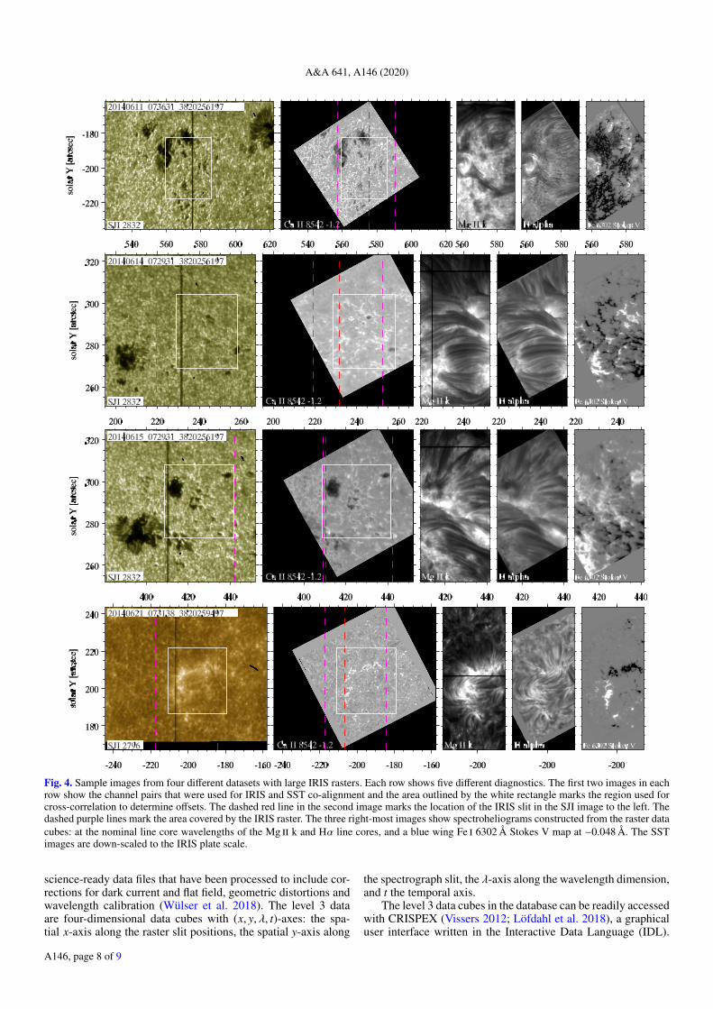
Fig. 4. Sample images from four different datasets with large IRIS rasters. Each row shows five different diagnostics. The first two images in eachrow show the channel pairs that were used for IRIS and SST co-alignment and the area outlined by the white rectangle marks the region used forcross-correlation to determine offsets. The dashed red line in the second image marks the location of the IRIS slit in the SJI image to the left. Thedashed purple lines mark the area covered by the IRIS raster. The three right-most images show spectroheliograms constructed from the raster datacubes: at the nominal line core wavelengths of the Mg ii k and Hα line cores, and a blue wing Fe i 6302 Å Stokes V map at −0.048 Å. The SSTimages are down-scaled to the IRIS plate scale.

science-ready data files that have been processed to include cor-rections for dark current and flat field, geometric distortions andwavelength calibration (Wülser et al. 2018). The level 3 dataare four-dimensional data cubes with (x, y, λ, t)-axes: the spa-tial x-axis along the raster slit positions, the spatial y-axis along

the spectrograph slit, the λ-axis along the wavelength dimension,and t the temporal axis.

The level 3 data cubes in the database can be readily accessedwith CRISPEX (Vissers 2012; Löfdahl et al. 2018), a graphicaluser interface written in the Interactive Data Language (IDL).

A146, page 8 of 9

L. H. M. Rouppe van der Voort et al.: High-resolution observations of the solar photosphere, chromosphere, and transition region

It allows for side-by-side browsing and basic time-series analy-sis of the IRIS rasters, SJIs and CRISP or CHROMIS data. TheCRISPEX interface is distributed as part of the IRIS packagein SolarSoft IDL and can also be downloaded4 separately; how-ever, it requires SolarSoft for full functionality when inspectingthe IRIS-SST data. Tutorials for its use are available online4,5.

Acknowledgements. This paper is dedicated to Ted Tarbell who passed away inApril 2019. Ted was the leader of the LMSAL SVST/SST campaigns since the1980s through the 2000s and participated with great enthusiasm in the LMSALcampaigns in 2013 and 2014. Ted was a great friend and an inspiring mentorto his junior colleagues. The Swedish 1 m Solar Telescope is operated on theisland of La Palma by the Institute for Solar Physics of Stockholm Universityin the Spanish Observatorio del Roque de los Muchachos of the Instituto deAstrofísica de Canarias. The Institute for Solar Physics is supported by a grantfor research infrastructures of national importance from the Swedish ResearchCouncil (registration number 2017-00625). IRIS is a NASA small explorer mis-sion developed and operated by LMSAL with mission operations executed atNASA Ames Research Center and major contributions to downlink communica-tions funded by ESA and the Norwegian Space Centre. We thank the followingpeople for their assistance at the SST: Jack Carlyle, Tiffany Chamandy, HenrikEklund, Thomas Golding, Chris Hoffmann, Charalambos Kanella, Ingrid MarieKjelseth, and Bhavna Rathore. We further acknowledge excellent support at theSST by Pit Sütterlin. We are also grateful to the IRIS planners for the IRIS-SSTcoordination. This project has received funding from the European Union’s Hori-zon 2020 research and innovation programme under grant agreement No 824135.This research is supported by the Research Council of Norway, project number250810, and through its Centres of Excellence scheme, project number 262622.BDP and colleagues at LMSAL and BAERi acknowledge support from NASAcontract NNG09FA40C (IRIS). JdlCR is supported by grants from the SwedishResearch Council (2015-03994), the Swedish National Space Agency (128/15)and the Swedish Civil Contingencies Agency (MSB). This project has receivedfunding from the European Research Council (ERC) under the European Union’sHorizon 2020 research and innovation programme (SUNMAG, grant agreement759548). VMJH and SJ receive funding from the European Research Coun-cil (ERC) under the European Union’s Horizon 2020 research and innovationprogramme (grant agreement No. 682462). JMS is supported by NASA grantsNNX17AD33G, 80NSSC18K1285, and NSF grant AST1714955. GV is sup-ported by a grant from the Swedish Civil Contingencies Agency (MSB). CFacknowledges funding from CNES. We made much use of NASA’s AstrophysicsData System Bibliographic Services.

ReferencesBose, S., Henriques, V. M. J., Joshi, J., & Rouppe van der Voort, L. 2019a, A&A,

631, L5Bose, S., Henriques, V. M. J., Rouppe van der Voort, L., & Pereira, T. M. D.

2019b, A&A, 627, A46Carlsson, M., Leenaarts, J., & De Pontieu, B. 2015, ApJ, 809, L30de la Cruz Rodríguez, J. 2019, A&A, 631, A153de la Cruz Rodríguez, J., Löfdahl, M. G., Sütterlin, P., Hillberg, T., & Rouppe

van der Voort, L. 2015, A&A, 573, A40de la Cruz Rodríguez, J., Leenaarts, J., Danilovic, S., & Uitenbroek, H. 2019,

A&A, 623, A74De Pontieu, B., Title, A. M., Lemen, J. R., et al. 2014a, Sol. Phys., 289, 2733De Pontieu, B., Rouppe van der Voort, L., McIntosh, S. W., et al. 2014b, Science,

346, 1255732Drews, A., & Rouppe van der Voort, L. 2020, A&A, 638, A63

4 https://github.com/grviss/crispex5 https://iris.lmsal.com/tutorials.html

Hansteen, V. H., Archontis, V., Pereira, T. M. D., et al. 2017, ApJ, 839, 22Henriques, V. M. J. 2012, A&A, 548, A114Leenaarts, J., Pereira, T. M. D., Carlsson, M., Uitenbroek, H., & De Pontieu, B.

2013a, ApJ, 772, 89Leenaarts, J., Pereira, T. M. D., Carlsson, M., Uitenbroek, H., & De Pontieu, B.

2013b, ApJ, 772, 90Lemen, J. R., Title, A. M., Akin, D. J., et al. 2012, Sol. Phys., 275, 17Löfdahl, M. G. 2002, in Society of Photo-Optical Instrumentation Engineers

(SPIE) Conference Series, eds. P. J. Bones, M. A. Fiddy, & R. P. Millane,Proc. SPIE, 4792, 146

Löfdahl, M. G., Henriques, V. M. J., & Kiselman, D. 2011, A&A, 533, A82Löfdahl, M. G., Hillberg, T., de la Cruz Rodriguez, J., et al. 2018, ArXiv e-prints

[arXiv:1804.03030]Martínez-Sykora, J., Rouppe van der Voort, L., Carlsson, M., et al. 2015, ApJ,

803, 44Martínez-Sykora, J., De Pontieu, B., Hansteen, V. H., et al. 2017, Science, 356,

1269Nóbrega-Siverio, D., Martínez-Sykora, J., Moreno-Insertis, F., & Rouppe van

der Voort 2017, ApJ, 850, 153Orozco Suárez, D., & Del Toro Iniesta, J. C. 2007, A&A, 462, 1137Ortiz, A., Hansteen, V. H., Bellot Rubio, L. R., et al. 2016, ApJ, 825, 93Ortiz, A., Hansteen, V. H., Nóbrega-Siverio, D., & van der Voort, L. R. 2020,

A&A, 633, A58Pereira, T. M. D., Leenaarts, J., De Pontieu, B., Carlsson, M., & Uitenbroek, H.

2013, ApJ, 778, 143Pereira, T. M. D., Carlsson, M., De Pontieu, B., & Hansteen, V. 2015, ApJ, 806,

14Pereira, T. M. D., Rouppe van der Voort, L., Hansteen, V. H., & De Pontieu, B.

2018, A&A, 611, L6Rathore, B., Carlsson, M., Leenaarts, J., & De Pontieu, B. 2015a, ApJ, 811, 81Rathore, B., Pereira, T. M. D., Carlsson, M., & De Pontieu, B. 2015b, ApJ, 814,

70Rouppe van der Voort, L., De Pontieu, B., Pereira, T. M. D., Carlsson, M., &

Hansteen, V. 2015, ApJ, 799, L3Rouppe van der Voort, L. H. M., Rutten, R. J., & Vissers, G. J. M. 2016, A&A,

592, A100Rouppe van der Voort, L., De Pontieu, B., Scharmer, G. B., et al. 2017, ApJ, 851,

L6Rutten, R. J., & Rouppe van der Voort, L. H. M. 2017, A&A, 597, A138Scharmer, G. B. 2006, A&A, 447, 1111Scharmer, G. B., Bjelksjö, K., Korhonen, T. K., Lindberg, B., & Petterson, B.

2003a, in Innovative Telescopes and Instrumentation for Solar Astrophysics,eds. S. L. Keil, & S. V. Avakyan, Proc. SPIE, 4853, 341

Scharmer, G. B., Dettori, P. M., Lofdahl, M. G., & Shand, M. 2003b, inInnovative Telescopes and Instrumentation for Solar Astrophysics, eds. S. L.Keil, & S. V. Avakyan, Proc. SPIE, 4853, 370

Scharmer, G. B., Narayan, G., Hillberg, T., et al. 2008, ApJ, 689, L69Scharmer, G. B., Löfdahl, M. G., Sliepen, G., & de la Cruz Rodríguez, J. 2019,

A&A, 626, A55Shine, R. A., Title, A. M., Tarbell, T. D., et al. 1994, ApJ, 430, 413Skogsrud, H., Rouppe van der Voort, L., & De Pontieu, B. 2016, ApJ, 817, 124van Noort, M., Rouppe van der Voort, L., & Löfdahl, M. G. 2005, Sol. Phys.,

228, 191Vissers, G. 2012, & Rouppe van der Voort. L., ApJ, 750, 22Vissers, G. J. M., Rouppe van der Voort, L. H. M., & Carlsson, M. 2015a, ApJ,

811, L33Vissers, G. J. M., Rouppe van der Voort, L. H. M., Rutten, R. J., Carlsson, M., &

De Pontieu, B. 2015b, ApJ, 812, 11Vissers, G. J. M., de la Cruz Rodríguez, J., Libbrecht, T., et al. 2019, A&A, 627,

A101Wülser, J. P., Jaeggli, S., De Pontieu, B., et al. 2018, Sol. Phys., 293, 149

A146, page 9 of 9