HIGH ORDER SPH-ALE METHODFOR HYDRAULIC TURBINE SIMULATIONS

G-A. Renaut, S. Aubert, J-C. Marongiu

LMFA UMR CNRS 5509, Ecole centrale de Lyon, Ecully, France, gilles-alexis.renaut@ec-lyon.fr

LMFA UMR CNRS 5509, Ecole centrale de Lyon, Ecully, France, stephane.aubert@ec-lyon.fr

ANDRITZ Hydro SAS, Villeurbanne, France, jean-christophe.marongiu@andritz.com

ABSTRACTThis paper describes the development of a high order meshless method for the simulation ofinviscid, weakly compressible, smooth and subsonic flows. The novelty of this approach is basedon the use of least squares fitting to compute the state at the interface in the numerical fluxreconstruction step. The main motivation of this work is to reduce the numerical dissipation inthe Riemann solver used to compute inviscid fluxes. A second aspect of this paper is to developan adaptive p-refinement in the frame of the SPH-ALE scheme i.e to adapt the order of thisreconstruction. Numerical simulations show the accuracy and the robustness of the numericalapproach for hydraulic turbines.

NOMENCLATURE

c0 numerical speed sound [m/s]Cp pressure coefficientd number of dimension in spaceD domain of influence of particleG numerical fluxh smoothing length or dilatation parameter of one particle [m]H Hessian matrixi index of the particle of interestj index of the neighbor of the particle i in Di

J weighted square residualM Least squares matrix. M = QR with Q orthonormal and R upper triangular matricesnij unit vector connecting the particles i and j oriented from i to jp order of the polynomial reconstructionP relative static pressure℘ polynomial basis for the least square reconstructiont time [s]v0 transport field [m/s]Wij kernel function evaluated for particles i and j [m−3]X = (X,1, · · · , X,d) vector position in <dXij position of the mid-point between the particles i and jα limiterεapp reconstruction error estimator (reference value is 10−4)∇ gradient operator

1

Proceedings of

11th European Conference on Turbomachinery Fluid dynamics & Thermodynamics

ETC11, March 23-27, 2015, Madrid, Spain

OPEN ACCESS

Downloaded from www.euroturbo.eu Copyright © by the Authors

ω measure of the volume of particle [m3]φ state value of one particleφh approximation of the state value φρ density of fluid [kg/m3] ( reference value ρ0 = 1000kg/m3)

INTRODUCTIONNowadays computational fluid dynamics (CFD) is routinely used for many applications in aero-

dynamics, hydromechanics and aerospace. Complex geometries are discretized by unstructured grids.Mesh based methods like high order continuous finite element methods (FEMs), discontinuous Galerkinmethods (DGMs) and finite volume methods (FVMs) have gained popularity for the numerical sim-ulation of compressible and incompressible Euler and Navier-Stokes equations. For reasons of ro-bustness and calculation cost, second-order schemes are routinely used for engineering problems.However, for a set of industrial applications, mesh-based methods are not always efficient and easy touse (free surface, moving geometries...).In 1977, the meshless SPH method (Smoothed Particle Hydrodynamics) was proposed by Lucy forastrophysical applications. Later, the SPH-ALE method was developed by Vila (1999). The mainidea of this variant of the SPH is to use Riemann solvers to compute numerical flux unlike classicalSPH approach where an artificial viscosity is used to stabilize the method (Monaghan,1985).The key issue in the development of high-order SPH-ALE schemes is the implementation of efficientreconstruction procedures of unknown variables at interface for each interaction. Indeed, the numer-ical dissipation due to the Riemann solver can be reduced with a MUSCL reconstruction (MonotoneUpwind Scheme for Conservation Laws) introduced for finite volume method by van Leer (1979).The idea is to replace the piecewise constant approximation of Godunov’s scheme by piecewise lin-ear reconstructed states. One can extend this approach with higher orders (p > 2). It is called ap-refinement. Another way to increase the accuracy of the results and to reduce the numerical dissi-pation is to use particles that have a size gradually reduced. It is a h-refinement where h representsthe particle size. In the finite element method, Babuska (1992) develops the idea to use both h and prefinements. A comparison between h and p refinements is presented in Li et al (2010) and shows thepossibility of a p-refinement for smooth flows.To obtain high order approximations in the frame of mesh-based method, and especially on unstruc-tured meshes the k-exact method is widely used (Haider, 2013), (Barth, 1993). The Moving LeastSquares method very famous in the meshless community is not really far from the k-exact method.The main difference lies in defining moments in the least squares matrix and in the iterative aspectof the k-exact method. The MLS method proposed by Lancaster and Salkauskas (1981) is used forsmoothing and interpolating scattered data. Indeed it is often used in the field of meshless meth-ods (Shobeyri et al, 2010) and in the field of unstructured Finite Volume (Chassaing, 2013). It isworth to notice that other alternative approaches were developed e.g. a hybridization between WENO(Weighted Essentially Non-Oscillatory) methods and MLS approximation was published to improvethe accuracy of the SPH-ALE method for compressible flow (Avesani, 2014).In the present work, a moving least square reconstruction using the recursive aspect of the k-exactmethod is used to show the ability of the p-refinement for the SPH-ALE method. The results of thep-refinement are compared with results obtained with the h-refinement. The rest of the paper is or-ganized as follows. The governing equations and the SPH-ALE method are introduced in the nextsection. In a following section, the least squares reconstruction is exposed. The last section containsthe numerical results where the proposed method is applied to inviscid weakly compressible flowfor different types of particles’ motion. Finally, some conclusions, remarks and an outlook to futureresearch are given.

2

GOVERNING EQUATIONS AND SPH-ALE METHODThe SPH-ALE method is based on a distribution of moving particles. The displacement of this

set of particles is a regular vector field v0. At time t, the particles coordinates are Xi(t) and theirvolumes are ωi(t). The following PDE in conservative form (Vila, 1999), (Vila and Lanson, 2008) isconsidered to model the time evolution of each particle position, volume and flow values:

dXi

dt= v0i,

dωi

dt= ωi

∑j∈Di

ωj(v0j − v0i)∇iWij,

d(ωiφi)dt

+ ωi∑

j∈Diωj2G(φi, φj, v0i, v0j, nij)∇iWij = ωiSi

(1)

The inviscid numerical flux G between two interacting particles i and j is composed of an euleriannumerical flux F along the nij direction and an ALE term where v0ij and φij are respectively thetransport velocity and the state at the interface: G(φi, φj, v0i, v0j, nij) = F (φi, φj, nij) − v0ij ⊗ φij .The source term S could include gravity and viscosity effects. The sum over the neighborhood of icorresponds to the discrete computation of the divergence operator in the SPH framework. The SPH-ALE method can be seen as a cell-centered ALE Godunov-type method. Indeed, two specificities ofthis method can be developed :

1. The numerical flux G at each interface is computed from a moving Riemann problem for-mulated at the middle-point between particles’ positions Xij . This flux analogous to a finitevolume flux includes a numerical viscosity. To increase the accuracy, G(φi, φj, v0i, v0j, nij) isreplaced by G(φij, φji, v0i, v0j, nij) where φij is an approximation of φ at Xij given by a Taylorexpansion from the point Xi.

2. This meshless method is connected with the notion of Arbitrary Lagrange Euler approximation.Indeed the value of the transport field v0 can be imposed independently of the flow velocity .If this field is set to zero, particles have an Eulerian motion. If the transport field is equal tothe flow velocity field, particles have a Lagrangian motion. Finally, if an arbitrary continuoustransport field is imposed, they are in an ALE motion.

For more details about the SPH-ALE method, the reader is referred to the paper of Vila (1999).

HIGH ORDER RECONSTRUCTION FOR SCATTERED DATAThe Taylor expansion corresponding to a quadratic (p=2) reconstruction is given as :

φhi (X) = φi +∇Ti φ(X −Xi) +

1

2(X −Xi)

THi(X −Xi) (2)

values ∇iφ and Hi are respectively the gradient and the Hessian matrix of the state variable φ evalu-ated atXi. In the original paper of Vila (1999) this expansion used to evaluate the state at the interfaceinvolves a gradient computed with a SPH approximation based on a convolution product. It appearsthat in general the geometrical disorder of the particles’ distribution is detrimental to the accuracy ofthis SPH approximation. Moreover the computation of derivative of order greater than 3 is complex.A central point in the development of higher-order methods (higher than second order) is a higher-order polynomial reconstruction of primitive variables φ within the control volumes. To achieve this,the MLS approach is based on a weighted least squares approximation over the neighboring data(Lancaster ,1981). These unknowns ∇iφ and Hi are found by minimizing per particle the sum ofweighted squared residuals defined by :

Ji =1

2

∑j∈Di

ωjWij[φj − φhi (Xj)]2 (3)

3

The weighing function is ωjWij , where Wij is the SPH kernel function centered on particle i. It hasthe isotropic compact support Di and it is evaluated for every neighbors of the particle i in Di. Di

defines the stencil of the least square fitting. These weight functions are often represented as functionof the distance between two particles. In the present work, a Wendland function C4 is used. Moredetails about the impact of the choice of those kernel functions are given in Khelladi (2011).

An algebraic system MA = B appears when the equation Eq 3 is derived and written in a matrixform. The vectorA contains the unknowns∇iφ andHi. The least squares matrix isM = CTW (X)Cand the right hand side vector is B = CTW (X)∆φ. The vector ∆φ is composed of differences ofstate between interacting particles i.e. φj − φi. The matrix M is symmetric and positive. The rowsof the matrix C correspond to the development in the polynomial basis ℘ for each neighbors. For a2D problem and an order of polynomial basis p, the basis is specified as : ℘ = [X,1, X,2]

T for p = 1and ℘ = [X,1, X,2, X

2,1, X,1X,2, X

2,2]T for p = 2. In order to preserve good numerical properties of

the matrix M , a scaled centered basis is used : (X −Xi)/hi (Randles ,1997).For example in a 2D case, the least square matrix for a linear reconstruction is given as :

M2,2 =

( ∑j∈Di

ωjWij(Xj,1−Xi,1

hi)2

∑j∈Di

ωjWij(Xj,1−Xi,1

hi)(Xj,2−Xi,2

hi)∑

j∈DiωjWij(

Xj,1−Xi,1

hi)(Xj,2−Xi,2

hi)

∑j∈Di

ωjWij(Xj,2−Xi,2

hi)2

)(4)

Numerical experience shows some geometrical configurations where it is impossible to solve thealgebraic problem because the matrix M becomes ill-conditioned. For example, the representation ofa quadratic polynomial basis in a truncated region is complicated by the lack of neighbors. To avoidthis problem, a recursive algorithm of least square reconstruction was created by Barth (1993) andextended by Haider (2013). The k-derivatives are computed from the previous k − 1 derivatives. Aderivative of order two can be interpreted as two successive derivatives of order one. The advantage isto solve smaller algebraic problems per particle respectively 2× 2 and 3× 3 for 2D and 3D problems.Furthermore, the least squares matrix corresponding to a linear approximation is less sensitive togeometrical configuration.

To complete the MUSCL approach a limitation of the derivatives is introduced. Currently, thereare many and various limitation techniques developed in mesh-based methods. A classical tool veryclose to unstructured finite volume inspired by Barth-Jespersen (1989) or Venkatakrishnan (1993) isused to avoid spurious oscillations. A parameter αi ∈ [0; 1] is computed to limit the extrapolation ofthe field φ for the particle i and Eq 2 becomes :

φhi (X) = φi + αi[∇Ti φ(X −Xi) +

1

2(X −Xi)

THi(X −Xi)] (5)

Numerical aspects :In the frame of moving particles interacting with rotating solid, a robust and accurate technique

of reconstruction is necessary whatever the geometric configuration is. Adaptivity and stability needto be discussed. On the other hand, as already mentioned in the introduction, there are two ways toreduce numerical dissipation : the first one is h-refinement and the second is p-refinement.

h-refinementThe h-refinement consists in reducing the particles size, what leads to decrease the size of the

dilation parameter h and to increase the number of particles. The distance between nodal values beingreduced, state discontinuities are weaker what reduces numerical viscosity. However this refinementincreases drastically the computational cost. Besides, the time step size decreases because of the CFLcondition that applies to explicit time integrators.

4

p-refinement : adaptivity in p-order and in d-spaceNumerical robustness of this refinement method is closely connected to the number of nearby

particles. The stencil is given by the compact support of the kernel function. It must be large enoughto avoid an ill-conditioned matrix M . For a pth order polynomial basis, the number of neighbor par-ticles must be higher than (p + 1)(p + 2)/2 and (p + 1)(p + 2)(p + 3)/6 respectively in 2D and 3D.If those numbers are not satisfied, p must be decreased, until p = 0 sometimes. To strengthen thestability of the method, the d-adaptivity was implemented to handle various geometrical configura-tions of neighborhood of particles (Liu, 2003). For example, a set of points primarily aligned alongthe x-axis cannot give information about the derivatives along the y and z-axis. A polynomial basisof adjustable dimension is selected through a QR decomposition of the matrix M , where M = QR.Indeed, the orthogonal dense matrix Q contains the vector of the basis ( QTQ = I). The coefficientsof the upper triangular matrix R can be seen as a decomposition of the matrix M in the basis Q. Inthe case where a diagonal term of R is too small the matrix M cannot be fully decomposed in thisbasis. In the case of aligned particles in 2D, the smallest of the diagonal terms is half of the other.The idea behind d-adaptivity in this case is to project the least squares problem in the remaining 1Dbasis. The gradient in the other orthogonal direction is set to zero.

The concept of the p-adaptivity is to use high-order only when it is necessary, to reduce the costof simulation without reducing the accuracy. To use adaptive p-refinement, a local approximationerror is formulated by the least-squares functional evaluation (Perazzo 2008). This a posteriori errorestimator is computed as : εapp = ||φj − φhi (Xj)||L2(Di)/||φj||L2(Di). It is intuitively clear that theregion where this indicator is high requires an increase of the reconstruction order, i.e adaptation. Forexample, a quadratic reconstruction (p=2) is necessary close to a leading edge of a solid body wheregradients are stiff. The notations are in the following section ”p = 1” and ”p = 2” are for linear andquadratic approximation respectively. The possibility to have local linear or quadratic approximationsin the same simulation depending on the local value of εapp is noted ”p = 1 or 2”.

NUMERICAL RESULTSIn the following, the advantage of the p-refinement will be demonstrated in the case of an inviscid

flow around a static symmetric NACA 0020 hydrofoil without incidence in 2D. Next, the robustnessof the method for dynamic simulation is analyzed for a flow around two moving NACA 0020 hy-drofoils. This test case shows the capacities of the p-refinement on a moving particles distributionfor an unsteady flow. Indeed the particles distribution adapts itself to the motion of solid boundariesin an ALE manner (Neuhauser, 2014). The third test case corresponds to an industrial simulationof a water jet impacting rotating Pelton buckets in 3D. This last test case is computed to assess themethod for more complex configurations (free surface, high dynamics on rotating geometry). For allthree configurations, an explicit third order Runge-Kutta time integrator is used and the maximumof p-refinement is fixed equal to 2. The Euler equations are used to model the flow. The system isclosed with a barotropic equation of the state to compute the relative pressure (Murnaghan, 1944):P (ρ) =

c20ρ0γ

[( ρρ0

)γ − 1] where c0 is the numerical sound speed, γ is taken equal to 7 and ρ0 is thereference density (ρ0 = 1000kg/m3). The speed of sound is conveniently reduced to obtain a largercomputational time step. It is chosen as c0 = 10Umax where Umax is the maximum expected fluidvelocity.

Static NACA hydrofoilThis test case is computed with two objectives in mind. The first one is to assess the advantages of

p-refinement over h-refinement. The second is to stress the robustness of the method of reconstruction

5

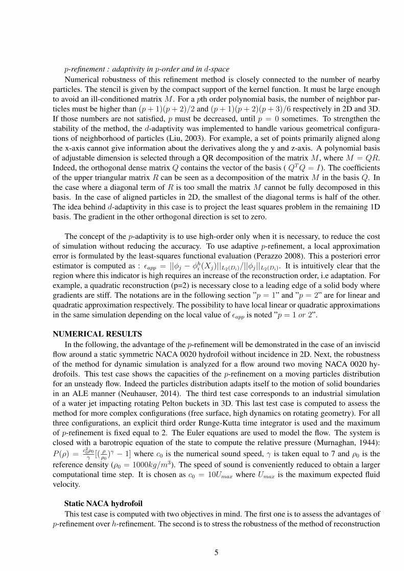
near the truncation of the computational domain due to the hydrofoil. The numerical Mach number is0, 1 with a velocity at inlet 2 m/s. The chord of the hydrofoil is equal to one meter and its thicknessis 20 % of chord. A refinement study is performed using a sequence of three distributions of points :N, 2N, 4N , i.e. respectively particles radius in {0, 02; 0, 0141; 0, 01} m. The distribution of points isobtained using the particle packing algorithm developed by Colagrossi (2012). The particles’ motionis Eulerian. The coarse distribution corresponds to N ≈ 69000 particles with 50 particles along thechord (Fig: 1b). The two finest distributions are obtained by refinement by

√2 and 2 the particles

radius. The farfield is situated 3 chords away from the leading and trailing edges. The velocity isimposed at the inlet and the pressure at the outlet. The top and bottom boundaries are periodic. Thechannel height is 6 m. The zero origin is at the middle of the chord.

(a) Velocity and pressure fields for N particles and p=1 (b) Focus for N (top) and 2N (bottom) particles

Figure 1: Results for a steady flow around a static hydrofoil in (a) and distribution of particles in (b).

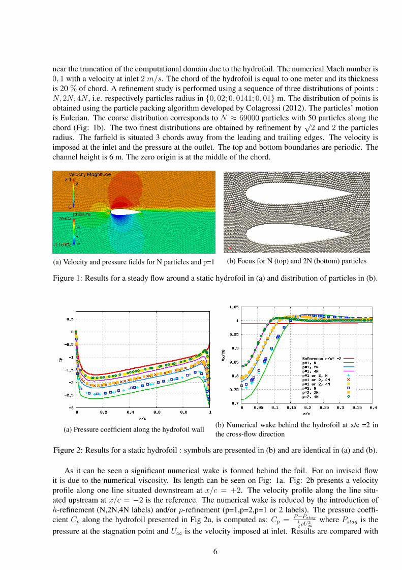
(a) Pressure coefficient along the hydrofoil wall(b) Numerical wake behind the hydrofoil at x/c =2 inthe cross-flow direction

Figure 2: Results for a static hydrofoil : symbols are presented in (b) and are identical in (a) and (b).

As it can be seen a significant numerical wake is formed behind the foil. For an inviscid flowit is due to the numerical viscosity. Its length can be seen on Fig: 1a. Fig: 2b presents a velocityprofile along one line situated downstream at x/c = +2. The velocity profile along the line situ-ated upstream at x/c = −2 is the reference. The numerical wake is reduced by the introduction ofh-refinement (N,2N,4N labels) and/or p-refinement (p=1,p=2,p=1 or 2 labels). The pressure coeffi-cient Cp along the hydrofoil presented in Fig 2a, is computed as: Cp = P−Pstag

12ρU2

∞where Pstag is the

pressure at the stagnation point and U∞ is the velocity imposed at inlet. Results are compared with

6

the potential solution computed with the freeware Xfoil (web.mit.edu/drela/Public/web/xfoil) for anisolated profile. It is to notice that the periodicity condition imposed on the top and bottom boundariesconfines the flow between two adjacent blades. The resulting acceleration contributes to decrease Cpvalues compared to the isolated profile configuration. An improvement of the pressure coefficientwith h and/or p refinement can be observed. The results converge to the potential solution. Adaptivep-refinement and full p-refinement shows very close results. The unphysical decrease of the Cp valueat the trailing edge can be explained by a feature of the SPH method. Indeed the numerical stencilextends in this region over the two sides of the hydrofoil and introduces artificial connectivities acrosssolid boundary. This aspect is not investigated in the present work.

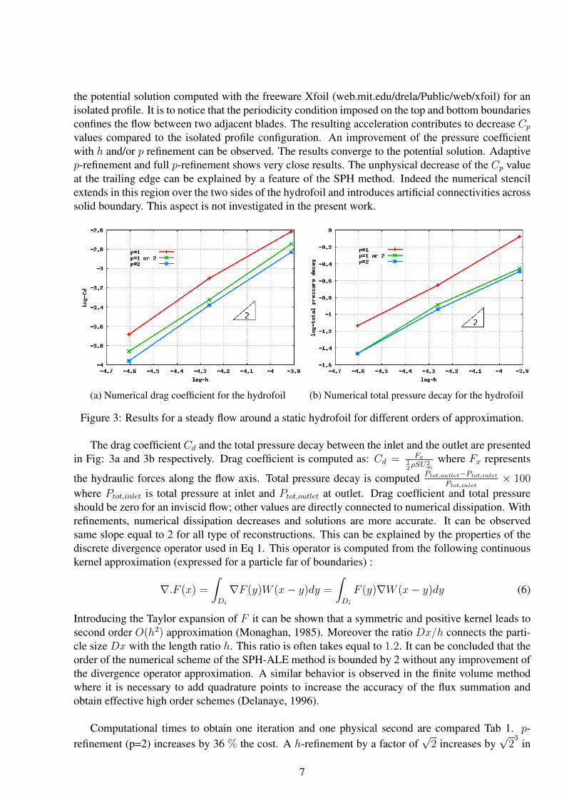
(a) Numerical drag coefficient for the hydrofoil (b) Numerical total pressure decay for the hydrofoil

Figure 3: Results for a steady flow around a static hydrofoil for different orders of approximation.

The drag coefficient Cd and the total pressure decay between the inlet and the outlet are presentedin Fig: 3a and 3b respectively. Drag coefficient is computed as: Cd = Fx

12ρSU2

∞where Fx represents

the hydraulic forces along the flow axis. Total pressure decay is computed Ptot,outlet−Ptot,inlet

Ptot,inlet× 100

where Ptot,inlet is total pressure at inlet and Ptot,outlet at outlet. Drag coefficient and total pressureshould be zero for an inviscid flow; other values are directly connected to numerical dissipation. Withrefinements, numerical dissipation decreases and solutions are more accurate. It can be observedsame slope equal to 2 for all type of reconstructions. This can be explained by the properties of thediscrete divergence operator used in Eq 1. This operator is computed from the following continuouskernel approximation (expressed for a particle far of boundaries) :

∇.F (x) =

∫Di

∇F (y)W (x− y)dy =

∫Di

F (y)∇W (x− y)dy (6)

Introducing the Taylor expansion of F it can be shown that a symmetric and positive kernel leads tosecond order O(h2) approximation (Monaghan, 1985). Moreover the ratio Dx/h connects the parti-cle size Dx with the length ratio h. This ratio is often takes equal to 1.2. It can be concluded that theorder of the numerical scheme of the SPH-ALE method is bounded by 2 without any improvement ofthe divergence operator approximation. A similar behavior is observed in the finite volume methodwhere it is necessary to add quadrature points to increase the accuracy of the flux summation andobtain effective high order schemes (Delanaye, 1996).

Computational times to obtain one iteration and one physical second are compared Tab 1. p-refinement (p=2) increases by 36 % the cost. A h-refinement by a factor of

√2 increases by

√23

in

7

2D the cost to achieve one physical second. The number of points multiplied by two and the CFLcondition explain this observation. Accordingly, p-refinement is much less expensive. p-adaptivity(p = 1 or 2) manages to reduce the computational cost compared to full p-refinement (by about 15%)but it is slightly more dissipative. An overall of h and p refinements gives the best results (p=2 and4N) on physical fields.

p=1 p=1 or 2 p=2N 2N 4N N 2N 4N N 2N 4N

CPU cost/iteration 1,00 1,99 4,00 1,19 2,33 4,81 1,36 2,70 5,44

CPU cost/second 1,00 2,81 8,01 1,19 3,29 9,63 1,36 3,81 10,87

Table 1: CPU time cost for h and p refinement (reference : p=1 ,N)

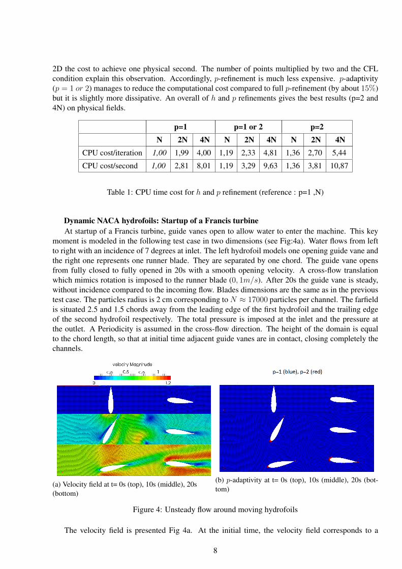
Dynamic NACA hydrofoils: Startup of a Francis turbineAt startup of a Francis turbine, guide vanes open to allow water to enter the machine. This key

moment is modeled in the following test case in two dimensions (see Fig:4a). Water flows from leftto right with an incidence of 7 degrees at inlet. The left hydrofoil models one opening guide vane andthe right one represents one runner blade. They are separated by one chord. The guide vane opensfrom fully closed to fully opened in 20s with a smooth opening velocity. A cross-flow translationwhich mimics rotation is imposed to the runner blade (0, 1m/s). After 20s the guide vane is steady,without incidence compared to the incoming flow. Blades dimensions are the same as in the previoustest case. The particles radius is 2 cm corresponding to N ≈ 17000 particles per channel. The farfieldis situated 2.5 and 1.5 chords away from the leading edge of the first hydrofoil and the trailing edgeof the second hydrofoil respectively. The total pressure is imposed at the inlet and the pressure atthe outlet. A Periodicity is assumed in the cross-flow direction. The height of the domain is equalto the chord length, so that at initial time adjacent guide vanes are in contact, closing completely thechannels.

(a) Velocity field at t= 0s (top), 10s (middle), 20s(bottom)

(b) p-adaptivity at t= 0s (top), 10s (middle), 20s (bot-tom)

Figure 4: Unsteady flow around moving hydrofoils

The velocity field is presented Fig 4a. At the initial time, the velocity field corresponds to a

8

velocity equal to 0 m/s in the computational domain. At t=10s, the unsteady velocity field begins tobecome more intense by the opening of the blade runner. The final time presented (t=20s) shows avelocity field for a fully opened channel. In Fig 4b, p-adaptivity can be observed close to the leadingand trailing edges where an adaptive higher order reconstruction is triggered (p=1 or 2). After 30s, theflow is stable and the guide vane is without incidence. Its drag coefficient for a linear approximation(p=1) is Cd = 0, 061 for N particles. By doubling the particles number, the drag coefficient decreasesto Cd = 0, 042. With p-adaptivity, its value for N particles drops to Cd = 0, 05 and Cd = 0, 045for full p-refinement (p=2). Again a reduction of numerical dissipation with p-refinement even withmoving particles can be observed.

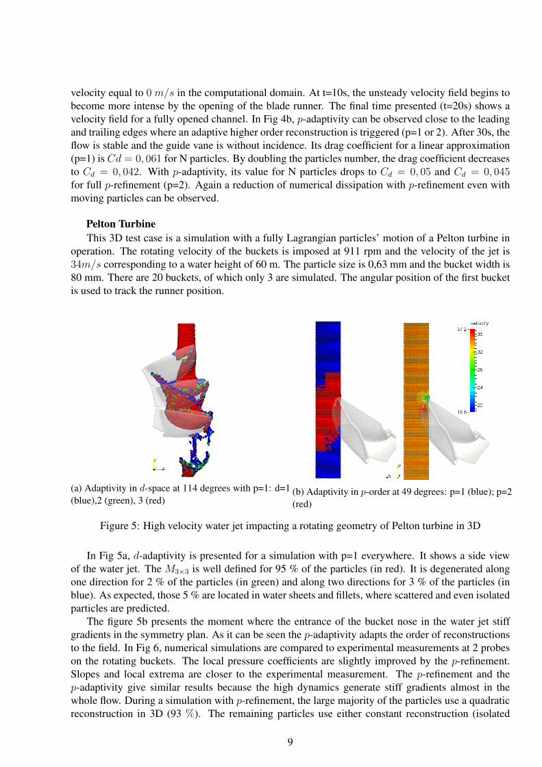
Pelton TurbineThis 3D test case is a simulation with a fully Lagrangian particles’ motion of a Pelton turbine in

operation. The rotating velocity of the buckets is imposed at 911 rpm and the velocity of the jet is34m/s corresponding to a water height of 60 m. The particle size is 0,63 mm and the bucket width is80 mm. There are 20 buckets, of which only 3 are simulated. The angular position of the first bucketis used to track the runner position.

(a) Adaptivity in d-space at 114 degrees with p=1: d=1(blue),2 (green), 3 (red)

(b) Adaptivity in p-order at 49 degrees: p=1 (blue); p=2(red)

Figure 5: High velocity water jet impacting a rotating geometry of Pelton turbine in 3D

In Fig 5a, d-adaptivity is presented for a simulation with p=1 everywhere. It shows a side viewof the water jet. The M3×3 is well defined for 95 % of the particles (in red). It is degenerated alongone direction for 2 % of the particles (in green) and along two directions for 3 % of the particles (inblue). As expected, those 5 % are located in water sheets and fillets, where scattered and even isolatedparticles are predicted.

The figure 5b presents the moment where the entrance of the bucket nose in the water jet stiffgradients in the symmetry plan. As it can be seen the p-adaptivity adapts the order of reconstructionsto the field. In Fig 6, numerical simulations are compared to experimental measurements at 2 probeson the rotating buckets. The local pressure coefficients are slightly improved by the p-refinement.Slopes and local extrema are closer to the experimental measurement. The p-refinement and thep-adaptivity give similar results because the high dynamics generate stiff gradients almost in thewhole flow. During a simulation with p-refinement, the large majority of the particles use a quadraticreconstruction in 3D (93 %). The remaining particles use either constant reconstruction (isolated

9

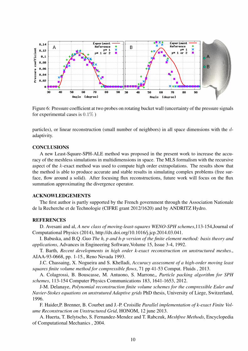
Figure 6: Pressure coefficient at two probes on rotating bucket wall (uncertainty of the pressure signalsfor experimental cases is 0.1% )

particles), or linear reconstruction (small number of neighbors) in all space dimensions with the d-adaptivity.

CONCLUSIONSA new Least-Square-SPH-ALE method was proposed in the present work to increase the accu-

racy of the meshless simulations in multidimensions in space. The MLS formalism with the recursiveaspect of the k-exact method was used to compute high order extrapolations. The results show thatthe method is able to produce accurate and stable results in simulating complex problems (free sur-face, flow around a solid). After focusing flux reconstructions, future work will focus on the fluxsummation approximating the divergence operator.

ACKNOWLEDGEMENTSThe first author is partly supported by the French government through the Association Nationale

de la Recherche et de Technologie (CIFRE grant 2012/1620) and by ANDRITZ Hydro.

REFERENCESD. Avesani and al, A new class of moving-least-squares WENO-SPH schemes,113-154,Journal of

Computational Physics (2014), http://dx.doi.org/10.1016/j.jcp.2014.03.041.I. Babuska, and B.Q .Guo The h, p and h-p version of the finite element method: basis theory and

applications, Advances in Engineering Software,Volume 15, Issue 3-4, 1992.T. Barth, Recent developments in high order k-exact reconstruction on unstructured meshes.,

AIAA-93-0668, pp. 1-15., Reno Nevada 1993.J.C. Chassaing, X. Nogueira and S. Khelladi, Accuracy assessment of a high-order moving least

squares finite volume method for compressible flows, 71 pp 41-53 Comput. Fluids , 2013.A. Colagrossi, B. Bouscasse, M. Antuono, S. Marrone,, Particle packing algorithm for SPH

schemes, 113-154 Computer Physics Communications 183, 1641-1653, 2012.J-M. Delanaye, Polynomial reconstruction finite volume schemes for the compressible Euler and

Navier-Stokes equations on unstrutured Adaptive grids PhD thesis, University of Liege, Switzerland,1996.

F. Haider,P. Brenner, B. Courbet and J.-P. Croisille Parallel implementation of k-exact Finite Vol-ume Reconstruction on Unstructured Grid, HONOM, 12 june 2013.

A. Huerta, T. Belytscho, S. Fernandez-Mendez and T. Rabczuk, Meshfree Methods, Encyclopediaof Computational Mechanics , 2004.

10

A. Iske, L. Bonaventura, E. Miglio, Kernel Based Vector Field Reconstruction in ComputationalFuild Dynamic Model,Int. J. Numer. Meth. Fluids 00:1-6 , 2000.

S. Khelladi, X. Nogueira, F. Bakir,I. Colominas Toward a higher order unsteady finite volumesolver based on reproducing kernel methods, Compt Methods Appl.Mech Engrg,2348-2362, 2011.

P. Lancaster, K. Salkauskas, Surfaces generated by moving least squares methods, Mathematicsof Computation, 87: 141-158, 1981.

Y. Li,S. Premasuthan and A. Jameson, Comparison of h- and p- Adaptations for Spectral Differ-ence Methods , 40th Fluid Dynamics Conference and Exhibit,Chicago, AIAA 4435 ,2010.

G. R. Liu Mesh free methods: moving beyond the finite element method, 4th ed., Vols. 1 and 2,CRC Press, London, 2003.

J.J. Monaghan and H. Pongracic, Artificial viscosity for particle methods, Applied NumericalMathematcis 1:187-194,1985.

F.D. Murnaghan, The Compressibility of Media under Extreme Pressures, Proceedings of theNational Academy of Sciences of the United States of America, vol. 30 1944, p. 244-247.

M. Neuhauser Development of a coupled SPH-ALE/Finite Volume method for the simulation oftransient flows in hydraulic machines PhD thesis in Ecole Centrale de Lyon, 2014 .

F. Perazzo , R. Lohner, L. Perez-Pozo, Adaptive methodology for meshless finite point method ,Advances in Engineering Software 39 156-166, 2008.

G. Shobeyri and M.H. Afshar, Simulating free surface problems using Discrete Least SquaresMeshless method, 113-154 Computers Fluids 39 461-470,2010.

J.P. Vila, On particle weighted methods and Smooth particle hydrodynamics, 3rd ed MathematicalModels and Methods in Applied Sciences, 1999.

V. Venkatakrishnan, On the accuracy of limiters and convergence to steady solutions , AIAA93-0880 Computer Sciences Corporation,1993.

11