American Economic Review 2017, 107(2): 305–330 https://doi.org/10.1257/aer.20141297

305

High Discounts and High Unemployment†

By Robert E. Hall*

Unemployment is high when financial discounts are high. In recessions, the stock market falls and all types of investment fall, including employers’ investment in job creation. The discount rate implicit in the stock market rises, and discounts for other claims on business income also rise. A higher discount implies a lower present value of the benefit of a new hire to an employer. According to the leading view of unemployment—the Diamond-Mortensen-Pissarides model—when the incentive for job creation falls, the labor market slackens and unemployment rises. Thus high discount rates imply high unemployment. (JEL E24, E32, E44, J23, J31, J63)

The point of this paper is that fluctuations in financial discounts play an important role in unemployment fluctuations.

The search-and-matching paradigm has come to dominate theories of move-ments of unemployment, because it has more to say about the phenomenon than merely interpreting unemployment as the difference between labor supply and labor demand. The ideas of Diamond, Mortensen, and Pissarides—henceforth, DMP—promise a deeper understanding of fluctuations in unemployment, most recently following the worldwide financial crisis that began in late 2008. But connecting the crisis to high unemployment according to the principles of the DMP model has proven a challenge.

In a nutshell, the DMP model relates unemployment to job creation incentives. When the payoff to an employer from taking on new workers declines, employers put fewer resources into recruiting new workers. Unemployment then rises and new workers become easier to find. Hiring returns to its normal level, so unemployment stabilizes at a higher level and remains there until job creation incentives return to normal. This mechanism rests on completely solid ground.

The question about the model that is unresolved today, more than 20 years after the publication of the canon of the model, Mortensen and Pissarides (1994), is: What force depresses the payoff to job creation in recessions? In that paper, and in

* Hoover Institution, Stanford University, Stanford, CA 94305 (e-mail: rehall@stanford.edu). The Hoover Institution supported this research. The research is also part of the National Bureau of Economic Research’s Economic Fluctuations and Growth Program. I am grateful to the referees and to Jules van Binsbergen, Gabriel Chodorow-Reich, John Cochrane, Steven Davis, Loukas Karabarbounis, Arvind Krishnamurthy, Ian Martin, Nicolas Petrosky-Nadeau, Leena Rudanko, Martin Schneider, and Eran Yashiv for helpful comments. The author declares that he has no relevant or material financial interests that relate to the research described in this paper.

† Go to https://doi.org/10.1257/aer.20141297 to visit the article page for additional materials and author disclosure statement.

306 THE AMERICAN ECONOMIC REVIEW fEbRuARy 2017

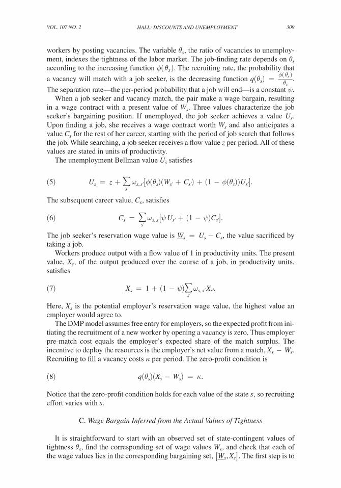
hundreds of successor papers, the force is a drop in productivity. But unemployment does not track the movements of productivity in US data, as Figure 1 shows.

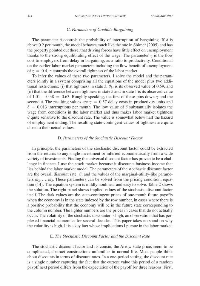
A more promising line of thought starts from the observation that discount rates rise dramatically in recessions—a recent paper by two financial economists finds “…value-maximizing managers face much higher risk-adjusted cost of capital in their investment decisions during recessions than expansions” (Lustig and Verdelhan 2012, p. S35). A long tradition in finance has emphasized that discounts vary over time: Rozeff (1984), Fama and French (1988), Campbell and Shiller (1988), and, recently, Cochrane (2011). Figure 2 suggests that the stock market and unemploy-ment respond to the same underlying forces, especially in the past few decades.

The causal chain I have in mind is that some event creates a financial crisis, in which risk premiums rise, so discount rates rise, asset values fall, and all types of investment decline. In particular, the value that employers attribute to a new hire declines on account of the higher discount rate. Investment in hiring falls and unem-ployment rises. The logic pursued here is that the flow of benefits from a newly hired worker has financial risk comparable to corporate earnings, so the dramatic increase in the market discount applied to earnings that occurred in the crisis implied simi-larly higher discounting of benefit flows accruing to employers from adding workers.

The proposition that the discount rate has a role in unemployment is not new. Rather, the paper’s contribution is to connect the issue of unemployment volatility to the finance literature on the volatility of discount rates in the stock market. This paper responds to the challenge in Mukoyama (2009), an early contribution focus-ing on discount volatility and the labor market. That paper showed that extreme variations in discounts would be needed to rationalize the observed volatility of

0.8

0.8

0.9

0.9

1.0

1.0

1.1

0

2

4

6

8

10

12

1948

Reciprocal of index of real output per w

orkerP

erce

nt o

f pop

ulat

ion 

wor

king

 or 

look

ing 

for 

wor

k

Unemployment rate(left scale) 

Output per worker(inverse, right scale) 

1954 1960 1966 1972 1978 1984 1990 1996 2002 2008 2014

Figure 1. Unemployment and Detrended Output per Worker, 1948–2015

307Hall: Discounts anD unemploymentVol. 107 no. 2

unemployment in the canonical DMP model. The response has two main elements: it refers to the finance literature that finds high volatility in discounts in the stock market and it drops the Nash bargain in the canonical model in favor of slightly less flexible wages.

As Shimer (2005) showed, the DMP model, with realistic parameter values, implies tiny movements in unemployment in response to large changes in produc-tivity. His finding carries over to other driving forces. This paper confirms Shimer’s finding for the discount rate as a driving force. Under Shimer’s assumptions about other parameter values—which I believe to be reasonable—cyclical fluctuations in job creation incentives facing employers in the DMP specification based on axi-omatic Nash bargaining are much too small to explain the large variations in labor market tightness and unemployment. The reason is that the wage bargain is quite sensitive to job seekers’ outside option of continuing to search rather than agree-ing to a bargain with a given employer. When unemployment is high, the outside option has a lower value and the wage is lower. As a result, job creation incentives are maintained—wage flexibility keeps unemployment near a constant value. Hall and Milgrom (2008) point out that it is not credible that a bargaining worker treats returning to search as the relevant alternative in bargaining. Rather, the alternative to an unsatisfactory wage offer is to make a counteroffer. The alternating-offer spec-ification can generate much larger fluctuations in job creation incentives. It results in less flexibility of wages in the face of changes in driving forces, though it is by no means the same as a fixed wage. In the canonical DMP specification, the share of the joint match surplus accruing to employers is a constant over the cycle, thanks to the assumption of Nash bargaining. In the credible bargaining specification, the share is procyclical.

Reciprocal of index of real value of the stock m

arket P

erce

nt o

f pop

ulat

ion 

wor

king

 or 

look

ing 

for 

wor

k

Unemployment rate(left scale) 

Stock market(inverse, right scale)  

0.0

0.5

1.0

1.5

2.0

2.5

3.0

3.5

0

2

4

6

8

10

12

1948 1954 1960 1966 1972 1978 1984 1990 1996 2002 2008 2014

Figure 2. Unemployment and the Real, Detrended Value of the S&P Stock Market Index, 1948–2015

308 THE AMERICAN ECONOMIC REVIEW fEbRuARy 2017

I. Labor Market Model

The model shows how variations in the discount rate are a driving force for unemployment fluctuations. The model describes a labor market under the influ-ence of volatile financial impulses and fluctuations in productivity that arise outside the model. There is no assumption that these influences are exogenous. Rather, the model shows what happens in the labor market when discounts for risky payoffs rise substantially. The paper takes no stand on why discounts are so volatile.

Although, in general equilibrium, the discount and the unemployment rate are jointly determined endogenous variables, I will discuss the model using the causal language of the effect of discounts on unemployment.

A. Financial Environment

The agents in the model participate in a financial system with a complete capital market. The states of the economy, denoted s , follow a Markov process with transi-tion matrix π s, s′ . In state s , the Arrow state price of consumption in a succeeding state s′ is π s, s′ β m s′ / m s . Here, β is an overall discount factor and m s is a state-contingent valuation, which would be marginal utility in a representative consumer economy. I normalize m 1 = 1 .

The productivity of the representative worker, x , grows stochastically, so it is not state-contingent. Its growth rate is state-contingent:

(1) g s, s′ = x ′ __ x .

Values are stated relative to the current value of productivity. For example, a flow payoff is written y s x , and y s is the amount of the payoff in productivity units. Its capital value, Y s x , satisfies the present value condition

(2) Y s x = ∑ s′ π s, s′ β m s′ __ m s y s′ x′.

Dividing both sides by x yields

(3) Y s = ∑ s′ ω s, s′ y s′ .

Here,

(4) ω s, s′ = π s, s′ β m s′ __ m s g s, s′

is the Arrow state price adjusted for productivity growth.

B. Turnover and Labor Market Frictions

The mechanics of the labor market follow the standard principles of DMP—see Mortensen and Pissarides (1994) and Shimer (2005). A fraction of the mem-bers of the fixed labor force are searching for work each period. Employers recruit

309Hall: Discounts anD unemploymentVol. 107 no. 2

workers by posting vacancies. The variable θ s , the ratio of vacancies to unemploy-ment, indexes the tightness of the labor market. The job-finding rate depends on θ s according to the increasing function ϕ( θ s ) . The recruiting rate, the probability that

a vacancy will match with a job seeker, is the decreasing function q( θ s ) = ϕ( θ s ) ____ θ s .

The separation rate—the per-period probability that a job will end—is a constant ψ .When a job seeker and vacancy match, the pair make a wage bargain, resulting

in a wage contract with a present value of W s . Three values characterize the job seeker’s bargaining position. If unemployed, the job seeker achieves a value U s . Upon finding a job, she receives a wage contract worth W s and also anticipates a value C s for the rest of her career, starting with the period of job search that follows the job. While searching, a job seeker receives a flow value z per period. All of these values are stated in units of productivity.

The unemployment Bellman value U s satisfies

(5) U s = z + ∑ s′ ω s, s′ [ϕ( θ s )( W s′ + C s′ ) + (1 − ϕ( θ s )) U s′ ] .

The subsequent career value, C s , satisfies

(6) C s = ∑ s′ ω s, s′ [ψ U s′ + (1 − ψ) C s′ ] .

The job seeker’s reservation wage value is W _ s = U s − C s , the value sacrificed by taking a job.

Workers produce output with a flow value of 1 in productivity units. The present value, X s , of the output produced over the course of a job, in productivity units, satisfies

(7) X s = 1 + (1 − ψ) ∑ s′ ω s, s′ X s′ .

Here, X s is the potential employer’s reservation wage value, the highest value an employer would agree to.

The DMP model assumes free entry for employers, so the expected profit from ini-tiating the recruitment of a new worker by opening a vacancy is zero. Thus employer pre-match cost equals the employer’s expected share of the match surplus. The incentive to deploy the resources is the employer’s net value from a match, X s − W s . Recruiting to fill a vacancy costs κ per period. The zero-profit condition is

(8) q( θ s )( X s − W s ) = κ.

Notice that the zero-profit condition holds for each value of the state s , so recruiting effort varies with s .

C. Wage Bargain Inferred from the Actual Values of Tightness

It is straightforward to start with an observed set of state-contingent values of tightness θ s , find the corresponding set of wage values W s , and check that each of the wage values lies in the corresponding bargaining set, [ W _ s , X s ] . The first step is to

310 THE AMERICAN ECONOMIC REVIEW fEbRuARy 2017

solve equation (8) for the wage values corresponding to the levels of labor market tightness θ s :

(9) W s = X s − κ _____ q( θ s )

.

Then solve the linear system comprising equations (5), (6), and (7) for the job seek-er’s state-contingent reservation wages, W _ s , and the values of productivity, X s , and check that each W s lies in the corresponding bargaining set.

The same logic applies to a proposed wage-setting rule W s . To validate the rule, solve for the implied θ s from equation (8) and then check that the wage lies in the resulting bargaining set.

D. Credible Bargaining

Data on tightness and productivity do not identify the structural wage- determination function, so it is interesting to consider models of the bargaining process that impose enough structure to identify specific parameters. The credible bargaining protocol, based on alternating offers, is a logical candidate. The canon-ical DMP model invoked the Nash bargaining model, but Shimer (2005) demon-strated that the Nash bargain made wages so responsive to driving forces that the tightness of the labor market—and thus the unemployment rate—hardly responded at all to driving forces of plausible volatility. Hall and Milgrom (2008) observed that the Nash bargain made the unrealistic implicit assumption that the option available to the two parties if they did not make a bargain is to forego making a match, in which case each loses a share of the surplus available from the match. When the market is slack and jobs are hard to find, the job seeker’s outside option has a low value and the bargained wage is correspondingly low, assuming the job seeker has bargaining power comparable to that of the employer. The low wage restores normal unemployment. The alternating-offer bargaining model of Rubinstein (1982) and Rubinstein and Wolinsky (1985) considers the credible option of making a coun-teroffer in response to an unsatisfactory offer from the counterparty. The credible bargaining equilibrium is less sensitive to conditions in the outside market and cor-respondingly more sensitive to costs of delay in bargaining.

Gale (1986) introduced a way to modulate the influence of outside conditions with alternating-offer bargaining. In our version of the model, we posit a probabil-ity δ that some event will prevent the achievement of the bargain and cause the job seeker and employer to abandon their efforts to form a match. The higher the value of δ , the more responsive is the wage to unemployment.

For reasons explained in Hall and Milgrom (2008), the unique Nash equilibrium of the alternating offer bargaining game occurs when both parties are indifferent between accepting a pending offer and making a counteroffer one bargaining period later. The indifference condition for the worker, when contemplating an offer W s E from the employer, against making a counteroffer of W s K , is

(10) W s E + C s = δ U s + (1 − δ) [z + ∑ s′ ω s, s′ ( W s′ K + C s′ ) ] .

311Hall: Discounts anD unemploymentVol. 107 no. 2

The similar condition for the employer is

(11) X s − W s K = (1 − δ) [−γ + ∑ s′ ω s, s′ ( X s′ − W s′ E ) ] .

I assume that the wage is the average of the two values:

(12) W s = 1 __ 2 ( W s E + W s K ) .

In equilibrium, the receiving party always accepts the first offer. The alternating-offer structure matters only through the off-equilibrium incentives it provides to the par-ties at the time of the first offer.

E. Equilibrium with Credible Bargaining

The state variable of the model, s , encodes the driving forces, which are the sto-chastic discounter M s, s′ = β m s′ / m s and productivity growth g s, s′ . An equilibrium is a set of vectors,

(13) { θ s , U s , C s , P s , W s E , W s K , W s },

solving equations (5), (6), (7), (8), (10), (11), and (12). Hall and Milgrom (2008) show that the equilibrium, conditional on the tightness values, θ s , exists and is unique.

II. Stock Market Model

The valuation model for the stock market, written analogously to the equations for the labor market, is

(14) P s = ∑ s′ ω s, s′ ( P s′ + d s′ ).

Here P s is the value of a portfolio, relative to productivity, and d s is the dividend earned by the portfolio, relative to productivity. In finance, the same equation divided by P s is often written as

(15) 1 = ∑ s′ ω s, s′ R s, s′ ,

where R s, s′ is the return ratio, ( P s′ + d s′ )/ P s .

III. Specification and Parameters

A. State Space

The model implies that each observable state-contingent variable should have the same value for all observations assigned to the same state. In practice, that goal is

312 THE AMERICAN ECONOMIC REVIEW fEbRuARy 2017

beyond reach. A finite record limits the number of states for which it is possible to estimate the transition probabilities π s, s′ . The hope is that for a well-chosen small number of states, the model still reasonably approximates the behavior of the unat-tainable model that matches the observed data.

For the labor market, the state needs to record the pronounced cyclical variable, tightness, θ s . For the stock market, the price/dividend ratio is an influential state variable based on its forecasting power for subsequent returns. As the basic theme of this paper predicts, the correlation of θ and P/d is fairly high. Accordingly, I constructed the state space by calculating the average of θ and P/d weighted by the inverses of their standard deviations, and then formed five equally populated bins based on that weighted average. I also removed an upward linear time trend in P/d . I used the data for the S&P 500 stock portfolio from Robert Shiller’s website (http://www.econ.yale.edu/~shiller/ ).

Table 1 shows the monthly transition matrix, and the average values by state, of tightness θ s and the price/dividend ratio, for the period from January 1948 through May 2015. Figure 3 shows the time series for labor market tightness, θ , and the values assigned by the state space bins, based on the averages of the of θ and P/d in each bin. The discretization based on the average index is reasonably successful. Figure 4 shows that the approach is somewhat less successful in the case of the price/dividend ratio.

The matrix of state-contingent values of productivity growth g s, s′ appears in the supporting spreadsheet for this paper. Consistent with the lack of a relation-ship between productivity growth and labor market tightness revealed in Figure 1, the state space captures the general growth of productivity but only part of its ran-domness. For reasons to be discussed shortly, the omission of part of the random movements in productivity has almost no effect on the conclusions about the role of discount movements in the determination of unemployment.

B. Parameters and Variable Values Common to the DMP Model and this Paper

Values and sources are: κ = 0.213 , the vacancy holding cost as a ratio to productivity, from Shimer (2005); η = 0.5 , the elasticity of the Cobb-Douglas matching function, from Petrongolo and Pissarides (2001); u = 0.055 , unemployment at the calibration point; ψ = 0.0345 , the monthly job separation rate, from Shimer (0.10 per quarter); θ ∗ = 0.59 , the ratio of vacancies to unemployment at calibration point, taken as the value in state 3;

Table 1—Monthly Transition Matrix among the States and Average Values of Tightness and the Price/Dividend Ratio by State

To state

1 2 3 4 5 Average θ Average P/d

1 0.907 0.093 0.376 2902 0.093 0.815 0.093 0.483 364

From state 3 0.093 0.820 0.087 0.592 4154 0.087 0.839 0.075 0.687 4855 0.080 0.920 1.006 576

313Hall: Discounts anD unemploymentVol. 107 no. 2

f = (1 − u)ψ/u , the monthly job-finding rate, from the stationary condition for unemployment; μ = ( θ ∗ ) −η f , the matching efficiency parameter, from the matching function; q ∗ = f/ θ ∗ , the vacancy-filling rate; and z = 0.4 , the flow value from unemployment as a ratio to productivity, from Shimer.

0.0

0.2

0.4

0.6

0.8

1.0

1.2

1.4

1.6

1948 20131953 1958 1963 1968 1973 1978 1983 1988 1993 1998 2003 2008

Figure 3. Time Series for Labor Market Tightness, θ , and Its Value Based on the State Space

0

100

200

300

400

500

600

700

800

900

1,000

1948 20131953 1958 1963 1968 1973 1978 1983 1988 1993 1998 2003 2008

Figure 4. Time Series for the Price/Dividend Ratio, P/d , and Its Value Based on the State Space

314 THE AMERICAN ECONOMIC REVIEW fEbRuARy 2017

C. Parameters of Credible Bargaining

The parameter δ controls the probability of interruption of bargaining. If δ is above 0.2 per month, the model behaves much like the one in Shimer (2005) and has the property pointed out there, that driving forces have little effect on unemployment thanks to the strong equilibrating effect of the wage. The parameter γ is the flow cost to employers from delay in bargaining, as a ratio to productivity. Conditional on the earlier labor market parameters including the flow benefit of unemployment of z = 0.4 , γ controls the overall tightness of the labor market.

To infer the values of these two parameters, I solve the model and the param-eters jointly in a system comprising all the equations of the model plus two addi-tional restrictions: (i) that tightness in state 3, θ 3 , is its observed value of 0.59, and (ii) that the difference between tightness in state 5 and in state 1 is its observed value of 1.01 − 0.38 = 0.63 . Roughly speaking, the first of these pins down γ and the second δ . The resulting values are γ = 0.57 delay costs in productivity units and δ = 0.013 interruptions per month. The low value of δ substantially isolates the wage from conditions in the labor market and thus makes labor market tightness θ quite sensitive to the discount rate. The value is somewhat below half the hazard of employment ending. The resulting state-contingent values of tightness are quite close to their actual values.

D. Parameters of the Stochastic Discount Factor

In principle, the parameters of the stochastic discount factor could be extracted from the returns to any single investment or inferred econometrically from a wide variety of investments. Finding the universal discount factor has proven to be a chal-lenge in finance. I use the stock market because it discounts business income that lies behind the labor market model. The parameters of the stochastic discount factor are the overall discount rate, β , and the values of the marginal-utility-like parame-ters m 2 , … , m 5 . These parameters can be solved from the pricing condition, equa-tion (14). The equation system is mildly nonlinear and easy to solve. Table 2 shows the solution. The right panel shows implied values of the stochastic discount factor itself. The dark values are the state-contingent prices of one-month future payoffs when the economy is in the state indexed by the row number, in cases where there is a positive probability that the economy will be in the future state corresponding to the column number. The lighter numbers are the prices in cases that do not actually occur. The volatility of the stochastic discounter is high, an observation that has per-plexed financial economics for several decades. This paper takes no stand on why the volatility is high. It is a key fact whose implications I pursue in the labor market.

E. The Stochastic Discount Factor and the Discount Rate

The stochastic discount factor and its cousin, the Arrow state price, seem to be complicated, abstract constructions unfamiliar in normal life. Most people think about discounts in terms of discount rates. In a one-period setting, the discount rate is a single number capturing the fact that the current value this period of a random payoff next period differs from the expectation of the payoff for three reasons. First,

315Hall: Discounts anD unemploymentVol. 107 no. 2

under normal conditions, all future payoffs tend to be valued below their expecta-tions through the general discount captured by the parameter β . Second, the econ-omy can be in a current state with high marginal utility, say state 1, so all of the discounts in M 1, s′ = β u s′ / u 1 are low and the future is heavily discounted. Third, payoffs that tend to be smaller in states where marginal utility is high suffer an addi-tional discount because they are risky.

In the setup in this paper, β is below one and the lower-numbered states have higher marginal utility, so the stochastic discounter places high discounts on the future when the economy is in those states. Thus the second factor is important in understanding the high general level of the discounts and also their high volatility. The third factor is present in the model of this paper, in the form of state-dependent productivity, but the volatility of productivity is fairly low. In effect, the model con-siders an open economy which has only a small domestic source of volatility but is embedded in a world economy with high volatility arising, for example, from large fluctuations in productivity of some large economies.

The one-period discount rate r y, s for a random payoff next period, y s′ , with market value Y s and expectation Y

– s , is the value that solves

(16) 1 ______ 1 + r y, s

= Y s __ Y – s .

See Cochrane (2011) for a complete discussion of the various ways that financial economics handles discounts. Note that while the stochastic discounter is univer-sal, the discount rate is payoff-specific. In general, it is contingent on the current state.

The sum of row s of the Arrow state-price matrix ω s, s ′ is the first future term in the infinite sum of values for the present value of productivity, X s (recall that the productivities themselves are all one). Thus the one-month-ahead discount r s satisfies

(17) 1 ____ 1 + r s

= ∑ s′ ω s, s′ .

The left panel of Table 3 shows these discounts for productivity calculated from the stochastic discount factor inferred earlier from the stock market.

Table 2—Parameters of the Stochastic Discount Factor Estimated from the Stock Market

β, monthly common

discount factor 0.993

Stochastic discount factor

Next month’s state

1 2 3 4 5

m 1 1.000 0.99 0.93 0.84 0.76 0.71 m 2 0.932 1.07 0.99 0.91 0.82 0.76 m 3 0.851 1.17 1.09 0.99 0.89 0.83 m 4 0.765 1.30 1.21 1.10 0.99 0.92 m 5 0.711 1.40 1.30 1.19 1.07 0.99

316 THE AMERICAN ECONOMIC REVIEW fEbRuARy 2017

F. Discounts Over the Life of a Job

Because jobs last 1/ψ = 29 months, on the average, the change in the one-month discount rate is not the full account of a discount shock. Following the shock, the economy gradually returns to its normal discount. A reasonable way to summa-rize the multi-month discount is to use the internal rate of return. For a future payoff stream y t+τ ≥ 0 valued by the stochastic discount factor at Y t , the overall discount rate r t by this definition is the unique root of the equation

(18) Y t = ∑ τ ( 1 ____

1 + r t )

τ E t y t+τ .

Let X – s (r) be the present value of the present and future productivity of a worker

when the economy is in state s , discounted at rate r . It can be calculated from the recursion

(19) X – s (r) = 1 + 1 − ψ ____

1 + r ∑ s′ π s, s′ g s, s′ X

– s′ (r).

The vector of state-contingent discount rates, r s , associated with the productivity stream of a worker, falling at rate ψ , but rising on account of stochastic productivity growth, is the solution to the equations

(20) X – s ( r s ) = X s , for s = 1, … , N.

Calculation of the N values of the discounts r s requires N separate solutions of a mildly nonlinear equation. The right panel of Table 3 shows the overall discount rate by state. The pattern is the same as for the one-month discount, but the range is not as large.

IV. Inferences Based on Observed Tightness, Productivity, and the Stochastic Discount Factor

This section studies data from the stock market and the labor market without invoking a structural wage-setting model. As discussed above, the first step is to calculate the state-contingent present value of a worker’s job-long productivity, X s ,

Table 3—Discounts for Productivity Based on the Stochastic Discount Factor Inferred from the Stock Market

One-month-ahead discounts Overall discounts

State

Discounted value of next month’s

productivityDiscount rate,

percent per monthDiscount rate,

percent per yearDiscount rate,

percent per year

1 0.989 1.12 13.5 12.22 0.993 0.72 8.7 10.23 0.995 0.48 5.8 8.34 0.999 0.10 1.2 5.95 1.001 −0.11 −1.3 4.4

317Hall: Discounts anD unemploymentVol. 107 no. 2

using the stochastic discount factor from the stock market. The second step is to use the actual values of labor market tightness, θ s , to calculate the implied present value of the state-contingent wage, W s , from the zero-profit condition. The third step is to verify that the wage lies in the parties’ bargaining set. Table 4 shows the results of these calculations. The present value of productivity rises modestly with higher-numbered states, because the discount is lower. Tightness is more sensitive to the falling discount and so rises substantially. The present value of the wage rises almost in proportion to the present value of productivity, but the gap widens quite a bit—the wage bargain gives the employer a larger sliver of the present value of productivity when it is higher. The job seeker’s reservation wage value rises by more than the increase in the wage value itself, because alternative jobs are easier to find. The right-most column of the table shows the fraction of the surplus accruing to the worker, calculated as [ W s − W _ s ]/[ X s − W _ s ]. The share falls from the high level of 0.87 in the worst times in state 1 to 0.72 in the best times in state 5. Because these numbers lie between zero and one, the wage remains within the bargaining set in all states.

The fifth column of Table 4 shows the job value, J s = X s − W s , the employer’s part of the match surplus. To see the basic mechanism in the model linking discount-ing to tightness, it is useful to focus on the zero-profit condition, written as

(21) θ s = ( μ __ κ J s ) 2 .

Under the calibration in this paper, with matching elasticity 0.5, the elasticity of θ with respect to the job value is 2, an important source of amplification of discount movements and other shocks.

Table 4 is instructive about the role of sticky wages in labor market volatility. Though the wage is sticky enough to explain the full extent of large fluctuations in tightness and thus unemployment, the elasticity of the wage with respect to the driv-ing force is close to 1: Between states 1 and 5, the present value of productivity rises by 0.157 log points while the wage rises by 0.154 log points, for an elasticity of 0.98. If an elasticity of 1 is taken as the benchmark of full flexibility, the basic DMP model under the Shimer calibration delivers virtually fully flexible wages. Shimer (2005), reported a similar relation between productivity and the Nash-bargained wage.

The results in this section show that the volatility of labor market tightness squares with the volatility of discounts inferred from the stock market, in the sense that there is a state-dependent sticky wage W s lying in the parties’ bargaining set, and not obviously violating standards of reasonability, that delivers large enough

Table 4—State-Contingent Values of Key Labor Market Variables

State Tightness, θ s

Present values Worker’s share of surplus

Productivity, X s Wage, W s

Job value, X s − W s

Reservation wage, W _ s

1 0.38 23.56 23.39 0.17 22.24 0.872 0.48 24.35 24.15 0.19 23.12 0.843 0.59 25.38 25.16 0.21 24.22 0.824 0.69 26.64 26.41 0.23 25.53 0.795 1.01 27.58 27.30 0.28 26.57 0.72

318 THE AMERICAN ECONOMIC REVIEW fEbRuARy 2017

fluctuations in the incentive to create jobs, measured by J s , to account for the vol-atility of tightness and thus of unemployment. The results say nothing about why the bargain takes this form and how the bargain would be different under altered circumstances. Answering those questions calls for a model of bargaining.

The basic channel linking the discount to labor market tightness is the following: A higher discount lowers the job value, as shown in Table 4—its direct effect is on the present value of productivity, X . The present value of the wage moves in the same direction as X , but less than in proportion. In this sense, the wage is sticky. Because the wage falls less than productivity, the job value, J , falls more than in proportion to the fall in X . Then the zero-profit condition in equation (21) shows that the elasticity of tightness with respect to J is two, providing further amplification of the effect of the higher discount.

V. Results with Credible Bargaining

Table 5 shows results of solving the model with credible bargaining, with inter-ruption rate δ = 0.013 and delay cost γ = 0.567 , and with the same inputs and non-bargaining parameters as Table 4. The values of all the variables are quite simi-lar to those derived without a wage-determination model in Table 4.

A. Responses to Discount Shocks

Figure 5 shows the path of a typical shock to the discount rate. Initially, the econ-omy is in state 3 with a discount rate of 8.3 percent per year. An adverse shock takes the economy to state 2, with a rate of 10.2 percent. The figure shows the expected discount rate in the following months, based on the Markov process’s evolving probabilities. Over the next four years, the economy gradually approaches its ergo-dic distribution, with an expected discount rate of 8.3 percent.

Figure 6 shows the response of labor market tightness to the adverse discount shock shown in Figure 5. The labor market slackens immediately and substantially, then gradually resumes its normal level. The dynamics resemble those of quick con-tractions and gradual recoveries of the US business cycle.

B. Unemployment

In the DMP class of labor market models, tightness θ is a jump variable and thus a function of the aggregate state of the economy. Unemployment, on the other hand,

Table 5—Results Based on Credible Alternating-Offer Bargaining

Present values

Worker’s share of surplusState Tightness, θ s Productivity, X s Wage, W s

Reservation wage, W _ s

1 0.35 23.56 23.40 22.21 0.882 0.44 24.35 24.16 23.08 0.863 0.59 25.38 25.16 24.22 0.824 0.80 26.64 26.39 25.57 0.775 0.98 27.58 27.30 26.56 0.73

319Hall: Discounts anD unemploymentVol. 107 no. 2

introduces another state variable, the unemployment rate u , whose law of motion in the DMP tradition is taken to be

(22) u t = (1 − f t−1 ) u t−1 + ψ(1 − u t−1 ).

Because of this complication, I have so far developed the idea in this paper in terms of tightness rather than unemployment. Now I show the implications for unemployment.

0

2

4

6

8

10

12

0

Per

cent

per

yea

r 

 

Years4321

Figure 5. Response of the Discount Rate to Its Own Shock

0

0.1

0.2

0.3

0.4

0.5

0.6

0.7

Rat

io o

f vac

anci

es to

une

mpl

oym

ent,

θ 

0Years

4321

Figure 6. Response of Labor Market Tightness to an Adverse Discount Impulse

320 THE AMERICAN ECONOMIC REVIEW fEbRuARy 2017

Figure 7 shows unemployment calculated from the credible bargaining model, using the job-finding rate f t = μ θ t η , based on the stochastic discount factor inferred from the stock market, and, to a small extent, on the observed fluctuations in the growth of productivity. The figure also shows the actual monthly unemployment rate. Except for missing the extremes of the Korean and Vietnam wars and the three major recessions, the model’s unemployment rate tracks the actual rate closely.

VI. Conclusions from the Model

With plausible parameter values, the model shows that the volatile stochastic discount factor inferred from the stock market, along with a very small contribu-tion from productivity growth, accounts for most of the observed movements of labor market tightness and unemployment. Financial economics has agreed that the volatility of the factor must be high but still lacks agreement on why it is high. The model embodies substantial countercyclical movements in the share of the surplus accruing to workers—the wage is sticky in the sense that job seekers get a bigger share when jobs are hard to find.

VII. Further Topics

A. The Job Value

The job value J is the present value, using the appropriate discount rate, of the flow benefit that an employer gains from an added worker, measured as of the time the worker begins the job. Information from the labor market—the duration of the typi-cal vacancy—reveals a financial valuation that is hard to measure in any other way.

0

2

4

6

8

10

12

1948 1983

Per

cent

of l

abor

forc

e

1953 1958 1963 1968 1973 1978 1988 1993 1998 2003 2008 2013

Figure 7. Unemployment from the Model and Actual Unemployment

321Hall: Discounts anD unemploymentVol. 107 no. 2

The labor market reveals the job value from the condition that J equals the cost of attracting a new hire, which is the per-period vacancy cost, κ , times the duration of the typical vacancy, 1/q : J = κ/q . JOLTS reports the hiring rate and number of vacancies. The vacancy filling rate q is the ratio of the two. Figure 8 shows the result of the calculation for the total private economy starting in December 2000, at the outset of JOLTS, through the beginning of 2015, stated as an index.

Figure 8 also shows the S&P 500 index of the broad stock market, stated as an index in productivity units. The S&P 500 includes about 80 percent of the value of publicly traded US corporations but omits the substantial value of privately held cor-porations. The similarity of the job value and the stock market value is remarkable. The figure strongly confirms the hypothesis that similar forces govern the market values of claims on jobs and claims on corporations. Direct measurement of the job value in years prior to JOLTS is not possible, but proxies constructed under assump-tions of no fluctuations in matching efficiency show periods of high correlation in earlier years.

Figure 9 shows indexes of job values for the industries reported in JOLTS. Large declines in job values occurred in every industry after the crisis, including health, the only industry that did not suffer declines in employment during the recession. The strikingly similar responses in diverse industries strongly supports the hypoth-esis that an aggregate driving force dominates the movements of the job value at the industry level. This evidence points in the direction of aggregate forces such as rising discounts in recessions.

B. Variation in the Separation Rate

Shimer followed Mortensen and Pissarides and their successors in positing a con-stant separation rate. Data on separations, from both JOLTS and the CPS, show

0.0

0.2

0.4

0.6

0.8

1.0

1.2

1.4

2000

Inde

x va

lue,

200

7 =

1

Stock market Job value

2002 2004 2006 2008 2010 2012 2014

Figure 8. Job Value from JOLTS and S&P Stock Market Index, 2001 through 2014

322 THE AMERICAN ECONOMIC REVIEW fEbRuARy 2017

cyclical variations. The separation rate enters DMP-style model in two ways. First, higher separations reduce the present value X that an employer receives from a hire, because the job ends sooner, and increases the present value C of a worker’s career after the end of a job. Second, higher inflows to unemployment result in higher unemployment for a given tightness and corresponding job-finding rate.

Table 6 shows the first set of effects in the credible bargaining model. The sec-ond column shows the state-contingent movements in the JOLTS separation rate, in percent per month. Separations are higher in strong labor markets. The five columns to the right show the corresponding solution of the model. Procyclical separations dampen the response of tightness for a given amount of wage stickiness, measured by the bargaining-interruption rate δ . To match the dispersion of actual tightness, measured as before as θ 5 − θ 1 , wages need to be stickier—the solved value of δ is 0.0024. Compared to the results in Table 5, the variation in the present value of productivity, X s , exogenous to the model, is smaller with countercyclical separa-tions. With a stickier wage than in the model with a constant separation rate, the model amplifies the smaller variations and comes close to matching the observed state-contingent movements in tightness.

0.0

0.2

0.4

0.6

0.8

1.0

1.2

1.4

1.6

2001

Inde

x of

job

valu

e

2003 2005 2007 2009 2011 2013

Figure 9. Job Value Indexes for 14 Industries

Table 6—Effects of Variation in the Separation Rate within the Credible Bargaining Model

State

Present values Worker’s share of surplus

Separation rate, ψ s Tightness, θ s

Productivity, X s Wage, W s

Reservation wage, W _ s

1 3.23 0.37 24.36 24.20 23.03 0.872 3.26 0.45 24.94 24.76 23.69 0.853 3.50 0.59 25.45 25.23 24.29 0.824 3.58 0.81 26.22 25.97 25.16 0.775 3.68 1.00 26.76 26.49 25.75 0.73

323Hall: Discounts anD unemploymentVol. 107 no. 2

With respect to the relation between tightness and unemployment, although the canonical DMP model assumes that all separations result in unemployment and that all inflows to unemployment are from employment, flows in the labor market are more complicated. Many separations are not followed by unemployment and many inflows to unemployment are not from separations. The inflow rate to unemploy-ment, ι t , can be measured by solving the law of motion,

(23) u t+1 = (1 − f t ) u t + ι t (1 − u t ).

Many authors refer to inflows to unemployment as “separations,” but it is useful to distinguish them from separations, which constitute all departures from jobs whether into unemployment, new jobs, or out of the labor force.

The model in this paper does not make the unemployment rate state-contingent. Rather, unemployment is a rapidly moving state variable with state-contingent driv-ing forces. With a job-finding rate in the range implied here, unemployment con-verges quickly to its stationary value, now in state-contingent form,

(24) u s ∗ = ι s ____ ι s + f s .

Table 7 shows the implications of incorporating variable inflow rates in the model of this paper. The second column shows the state-contingent tightness from Table 6. The third column shows the inflow rate, which is quite countercyclical. Comparison of the fourth and fifth columns shows that taking account of higher inflows to unemployment in slack markets considerably increases the volatility of unemployment.

C. Role of Productivity Fluctuations in the Volatility of Tightness

The model incorporates observed fluctuations in the growth of productivity. To illustrate the role of productivity growth in the model, I set the growth rate of pro-ductivity, g s, s′ , to the average growth rate of productivity, in place of its actual empir-ical dependence on the states. The solution is almost identical to the solution with state-contingent productivity growth—none of the differences in state-contingent tightness θ s differs by more than 0.01. Thus productivity growth has essentially

Table 7—Labor Market Volatility with State-Contingent Inflow Rate to Unemployment

State Tightness

Monthly inflow rate to

unemployment

Stationary unemployment rate, percent

With constant inflow rate

With variable inflow rate

1 0.37 4.06 7.0 8.02 0.45 3.74 6.4 6.73 0.59 3.43 5.6 5.54 0.81 3.22 4.8 4.45 1.00 3.19 4.4 4.0

324 THE AMERICAN ECONOMIC REVIEW fEbRuARy 2017

no effect on the endogenous variables of the model. The reason is that the model incorporates the finding of Chodorow-Reich and Karabarbounis (2016) that the opportunity cost of work, z , is constant in productivity units. Without any changes in payoffs of nonwork relative to the payoff to work, the model has almost no scope to generate unemployment fluctuations from productivity fluctuations. This paper, accordingly, does not address the “Shimer puzzle” but rather follows the evidence that implies that productivity has no significant role in the volatility of labor market tightness.

D. Higher Opportunity Cost of Employment, z

Shimer (2005) took the opportunity cost of employment, z , (also called the flow benefit of unemployment), to be 0.4 productivity units. No conclusive evidence has yet emerged about the value of this parameter. Solving the model with a higher value, z = 0.6 , illustrates some of the properties of the credible bargain. Recall that the solution requires matching two moments of the five values of tightness, so as a practical matter there is no difference in tightness between models with z = 0.4 and z = 0.6 . Because both models satisfy the same zero-profit condition with the same values of X s , the present values of the bargained wage, W s , will also be the same. In the new solution, a drop of just under 0.2 in the delay cost of the employer, γ , essentially offsets the role of the higher z in the bargaining game itself, as captured by equations (10) and (11), except for the term δ U s . The parameter z appears by itself in equation (5), so an increase in that parameter has a direct positive effect on the unemployment value U s , which then would increase the bargained wage through the δ U s in equation (10). To offset that increase, δ is smaller—it is 0.0057. Wage stickiness is greater with the higher z , in the sense that the bargaining interruption rate is lower. The bargained wage is the same as in the lower- z economy, because the larger movements in the unemployment value with the higher z receive lower weight δ in the bargaining process.

E. Higher Vacancy Cost, κ

With a higher vacancy cost κ and prescribed values of tightness, the zero-profit condition, equation (8) requires a lower wage in every state. Equations (5) and (6) require that the unemployment values U s and the future career value C s be corre-spondingly lower. As in the case of a higher z , a lower interruption rate δ , operating through the term δ U s , achieves that reduction. The value of δ is 0.0069. Wage stick-iness is greater with a higher vacancy cost.

F. Other Measures of the Discount Rate in the Stock Market

An intuitive but not quite obvious result of finance theory is that the discount rate for a future cash flow is the expected rate of return to holding a claim to the cash flow. The issue of the expected return or discount rate on broad stock mar-ket indexes has received much attention in financial economics over the past three decades. Cochrane (2011) recently reviewed the issue. Research on this topic has found that two variables, the level of the stock market and the normalized level of

325Hall: Discounts anD unemploymentVol. 107 no. 2

consumption, are reliable forecasters of the return to an index such as the S&P. The top graph in Figure 10 shows the one-month ahead forecast from a regression where the left-hand variable is the one-month real return on the S&P and the right-hand variables are the ratio of the S&P at the beginning of the month to its dividends averaged over the prior year and the ratio of real consumption to disposable income in the month prior to the beginning of the period. The returns are stated at annual percent rates. The graph is quite similar to Figure 3 in Cochrane’s paper for his

Markov model

Campbell-Shillerregression

−10

−5

0

5

10

15

20

25

30

1959

Livingston panel

Markov model

1964 1969 1974 1979 1984 1989 1994 1999 2004 2009 2014

−10

−5

0

5

10

15

20

25

30

1959 1964 1969 1974 1979 1984 1989 1994 1999 2004 2009 2014

Figure 10. Measured Discounts for the S&P 500 Stock Price Index

326 THE AMERICAN ECONOMIC REVIEW fEbRuARy 2017

equation that includes consumption. The graph also shows the forecasts from the Markov setup of this paper. The forecasted return is

(25) ∑ s′ π s, s ′ R s, s′ − 1,

stated as an annual percent. The two approaches agree on some important periods: low discounts in the late 1960s and especially in the late 1990s, high discounts in the early 1960s, late 1970s through 1994, and especially in the financial crisis start-ing in late 2008. There are some periods of disagreement, mostly that the model finds its highest discounts in recessions—1974–1975, 1980, and 1981–1982, and 1990—without concurrence from the regression forecast. The two agree about the recessions of 2001 and 2007–2009.

G. The Short-Term Real Interest Rate

The short-term real return ratio, stated in units of productivity, R f, s , should satisfy the standard pricing condition,

(26) 1 = ∑ s′ ω s, s ′ R s, s′ , for all s.

The usual practice in finance is to include this condition among those to be satisfied by a stochastic discount factor. My attempts to solve for the factor with the 5-state setup of this paper were unsuccessful—several values of the state-contingent prices were negative. Consequently, I permit errors, shown in Table 8, for the pricing of one-year Treasury bills.

Another source of evidence on the volatility of expected returns in the stock mar-ket comes from the Livingston survey, which records professional forecasts of the S&P stock price index. It is shown in the bottom graph in Figure 10. As with the regression forecasts, there are periods of agreement with the Markov forecasts and periods of disagreement.

VIII. Concluding Remarks

The suggestion in this paper that the stock market and unemployment move together because of the common role of the discount rate is not new. Still, most recent research in the now-dominant DMP framework concentrates on productiv-ity as the driving force. The conclusion of this paper with respect to fluctuations in productivity is the following: because the evidence favors sticky wages in the sense of insulation of the wage bargain from tightness, if productivity fell by one or two percentage points while the flow value of unemployment, z , remained unchanged, unemployment would rise sharply. But the finding of Chodorow-Reich and Karabarbounis (2016) is that z falls in proportion to productivity, implying that such a decline in productivity has little effect on unemployment. I believe that no researcher has tried to make the case that any actual decline in productivity occurred following the financial crisis is anywhere near large enough or timed in the right way

327Hall: Discounts anD unemploymentVol. 107 no. 2

to explain the high and lingering unemployment rate in the United States, much less in countries like Spain where unemployment rose into the 20-percent range.

The novelty in this paper is its connection with the finance literature that quan-tifies the large movements in the discount rates in the stock market. This literature has reached the inescapable conclusion that the large movements in the value of the stock market arise mainly from changes in discount rates and only secondarily from changes in the dividend or profit flow capitalized in the stock market. The field is far from agreement on the reasons for the volatility of discount rates.

In view of these facts, it seems close to irresistible to conclude that whatever forces account for wide variations in the discount rates in the stock market also apply to the similar valuation problem that employers face when considering recruiting. A plunging stock market and a soaring unemployment rate go together.

IX. Related Research

Yashiv (2000) undertook the task of forming the present value of the difference between a worker’s marginal product and wage. Equation (4) in his paper is equiv-alent to equation (8) here. On page 492, Yashiv notes the analogy between the val-uation of a worker’s net contribution and valuation in the stock market of a stream of dividends. One important difference between his approach and mine is that he takes the hiring cost to be strongly convex in the flow of hires at the level of the firm, whereas I adopt the linearity that is the standard property of the DMP class of models. Under linearity, the asset value of the employment relationship is observed directly. By contrast, Yashiv uses GMM to infer the marginal hiring cost. A second important difference is that Yashiv’s approach does not distinguish between hiring costs incurred prior to a wage bargain and those following the bargain.

Merz and Yashiv (2007) study investment, hiring, and the stock market jointly. Adjustment costs for both inputs result in values of Tobin’s q for both inputs. They estimate a three-equation system comprising dynamic first-order conditions for investment and hiring and the equality of the market value of the firm to its capital stock and employment level valued by their respective q s. They find a high correla-tion of their fitted value of the US corporate sector with the actual value.

The relation between Merz and Yashiv’s work and the approach in this paper is that they rely on the strong assumption that the market value of a firm arises solely from its investments in plant, equipment, and employees. This paper makes the weaker assumption that corporate profits arise from many sources, including capital stocks, and uses evidence about how the stock market discounts the profit stream to

Table 8—Pricing Errors for 1-Year Treasury Bills and Implied Liquidity Premiums

StatePresent value of 1-month

future returnAnnual percentage liquidity

premium

1 0.9891 13.12 0.9924 9.13 0.9939 7.34 0.9984 1.95 1.0005 −0.5

328 THE AMERICAN ECONOMIC REVIEW fEbRuARy 2017

rationalize the observed value of one element of the one part of the profit flow, that arises from the pre-bargain investment that employers make in recruiting workers.

Yashiv (2016) extends his earlier work using a similar specification for joint adjustment costs of investment and hiring. In place of employment levels, the spec-ification uses hiring flows, capturing gross rather than net additions to employment. The hiring costs combine a quadratic term and a DMP-style vacancy holding cost. He computes a Campbell-Shiller-style decomposition of the returns on capital and labor that confirms the importance of variations in discount rates. The paper holds out the promise of helping DMP-type models better characterize the flow value of a newly hired worker to a firm.

Yashiv (2015) pursues the topic of a countercyclical job value in a number of ways. The paper contains a detailed review of the recent literature on employment volatility.

Kehoe, Midrigan, and Pastorino (2016) follows up the basic idea in this paper by considering the amplification of the discount effect that arises if the cash flows from a new hire are backloaded. The paper derives the volatility of the discount from financial frictions.

Schaal (2015) investigates issues that are complementary to those in this paper. His model has no aggregate uncertainty. Capital markets are incomplete, so idiosyn-cratic shocks are important. The labor market operates on the principle of directed search in contrast to the random search of the DMP model. Time-varying idiosyn-cratic risk is an important driving force of aggregate fluctuations, though the paper concludes that it can only account for about 40 percent of the increase in unemploy-ment following the crisis.

Schoefer (2015) finds discount effects on hiring that arise in financially con-strained firms when they honor commitments to pay wages negotiated in earlier, better times.

Kudlyak (2014) uses micro data on workers’ earnings to measure the present value of wages as of the time of hire. Wages of new hires are cyclical but once hired, wages don’t change much. Employers benefit from the low wages in slumps for many subsequent years. The paper takes an integrated approach to measuring the combined effects using longitudinal data for individual workers. It finds that a 1 percentage point increase in unemployment lowers the effective cost of labor by 5.2 percent, with a standard error of 0.8. This finding implies that the incentive to hire in weak markets is really strong and eliminates sticky wage explanations of the volatility of unemployment. It greatly deepens the mystery of the large increases in unemployment in recessions, when labor becomes a true bargain. Basu and House (2016) survey a large body of work on wage flexibility, concluding that the wage measure that controls employment volatility—Kudlyak’s or close relatives—is remarkably flexible. In the light of these findings, it appears that macroeconomics needs to identify an offsetting disadvantage to hiring during slumps to explain the existence and persistence of high unemployment.

Phelps (1994) considers the issue of the effect of variations in interest rates on employment in a different, non-DMP framework.

Gourio (2012) builds a model where a small probability of a disaster generates substantial variations in discounts, which influence employment through a standard labor-supply setup. The model does not include unemployment.

329Hall: Discounts anD unemploymentVol. 107 no. 2

Kuehn, Petrosky-Nadeau, and Zhang (2013) is an ambitious general-equilibrium model that combines a DMP labor market with a full treatment of financial markets. Its goal is roughly the reverse of the goal of this paper. It makes the case that volatil-ity in real allocations resulting from amplification of productivity shocks in the labor market causes financial volatility. In particular, the model can generate episodes that look like financial crises, with dramatic widening of the equity premium. The paper provides an endogenous source of economic disasters, an advance over the existing literature that takes large declines in output and consumption to be the result of exogenous collapses of productivity.

Kuehn and coauthors build in a number of the ideas from the post-Shimer lit-erature to gain high amplification in the labor market from productivity shocks. These include (i) adding a fixed cost to the pre-bargain recruiting cost, on top of the cost that varies with the time required to fill a job; (ii) assigning the worker a tiny bargaining weight; and (iii) assigning a high value to the worker’s activities while unemployed, apart from the value of search. They also build in ideas from modern finance that generate a high and variable equity premium along with a low and stable real interest rate. These are (i) an extremely high coefficient of relative risk aversion and (ii) a quite high elasticity of intertemporal substitution. The paper briefly surveys related earlier contributions linking asset-price volatility to unem-ployment volatility: Danthine and Donaldson (2002), Uhlig (2007), Gourio (2007), and Favilukis and Lin (2012).

Farmer (2012) noted the relationship between the levels of the stock market and unemployment. He adopts the traditional view that unemployment is simply the dif-ference between labor supply and demand, thus sidestepping the issues considered in this paper.

Kilic and Wachter (2015) build a model with a DMP labor market with an ad hoc sticky-wage specification, in which changes in discounts are the result of the influence of rare events.

Belo, Lin, and Bazdresch (2014) find that firms that hire large numbers of work-ers have lower subsequent returns in the stock market. This finding coincides with the idea in this paper—hiring efforts expand under situations with low discounts.

Hall (2016) surveys a broader literature relevant to the topics of this paper.

REFERENCES

Basu, Susanto, and Christopher L. House. 2016. “Allocative and Remitted Wages: New Facts and Challenges for Keynesian Models.” National Bureau of Economic Research Working Paper 22279.

Belo, Frederico, Xiaoji Lin, and Santiago Bazdresch. 2014. “Labor Hiring, Investment, and Stock Return Predictability in the Cross Section.” Journal of Political Economy 122 (1): 129–77.

Campbell, John Y., and Robert J. Shiller. 1988. “The Dividend-Price Ratio and Expectations of Future Dividends and Discount Factors.” Review of Financial Studies 1 (3): 195–228.

Chodorow-Reich, Gabriel, and Loukas Karabarbounis. 2016. “The Cyclicality of the Opportunity Cost of Employment.” Journal of Political Economy 124 (6): 1563–1618.

Cochrane, John H. 2011. “Presidential Address: Discount Rates.” Journal of Finance 66 (4): 1047–108.Danthine, Jean-Pierre, and John B. Donaldson. 2002. “Labour Relations and Asset Returns.” Review

of Economic Studies 69 (1): 41–64.Fama, Eugene F., and Kenneth R. French. 1988. “Dividend Yields and Expected Stock Returns.” Jour-

nal of Financial Economics 22 (1): 3–25.Farmer, Roger E. A. 2012. “The Stock Market Crash of 2008 Caused the Great Recession: Theory and

Evidence.” Journal of Economic Dynamics and Control 36 (5): 693–707.

330 THE AMERICAN ECONOMIC REVIEW fEbRuARy 2017

Favilukis, Jack, and Xiaoji Lin. 2012. “Wage Rigidity: A Solution to Several Asset Pricing Puzzles.” Charles A. Dice Center Working Paper 2012–16.

Gale, Douglas M. 1986. “Bargaining and Competition Part I: Characterization.” Econometrica 54 (4): 785–806.

Gourio, François. 2007. “Labor Leverage, Firms’ Heterogeneous Sensitivities to the Business Cycle, and the Cross-Section of Expected Returns.” http://sites.google.com/site/fgourio/ (accessed Decem-ber 1, 2016).

Gourio, François. 2012. “Disaster Risk and Business Cycles.” American Economic Review 102 (6): 2734–66.

Hall, Robert E. 2016. “Macroeconomics of Persistent Slumps.” National Bureau of Economic Research Working Paper 22230.

Hall, Robert E. 2017. “High Discounts and High Unemployment: Datasets.” American Economic Review. https://doi.org/10.1257/aer.20141297.

Hall, Robert E., and Paul R. Milgrom. 2008. “The Limited Influence of Unemployment on the Wage Bargain.” American Economic Review 98 (4): 1653–74.

Kehoe, Patrick, Virigiliu Midrigan, and Elena Pastorino. 2016. “Debt Constraints and Employment.” NBER Working Paper 22614.

Kilic, Mete, and Jessica A. Wachter. 2015. “Risk, Unemployment, and the Stock Market: A Rare-Event-Based Explanation of Labor Market Volatility.” National Bureau of Economic Research Working Paper 21575.

Kudlyak, Marianna. 2014. “The Cyclicality of the User Cost of Labor.” Journal of Monetary Econom-ics 68: 53–67.

Lustig, Hanno, and Adrien Verdelhan. 2012. “Business Cycle Variation in the Risk-Return Trade-Off.” Journal of Monetary Economics 59: S35–S49.

Merz, Monika, and Eran Yashiv. 2007. “Labor and the Market Value of the Firm.” American Economic Review 97 (4): 1419–31.

Mortensen, Dale T., and Christopher A. Pissarides. 1994. “Job Creation and Job Destruction in the Theory of Unemployment.” Review of Economic Studies 61 (3): 397–415.

Mukoyama, Toshihiko. 2009. “A Note on Cyclical Discount Factors and Labor Market Volatility.” https://sites.google.com/site/toshimukoyama/ (accessed December 1, 2016).

Petrongolo, Barbara, and Christopher A. Pissarides. 2001. “Looking into the Black Box: A Survey of the Matching Function.” Journal of Economic Literature 39 (2): 390–431.

Petrosky-Nadeau, Nicolas, Lu Zhang, and Lars-Alexander Kuehn. 2013. “Endogenous Disasters and Asset Prices.” Charles A. Dice Center Working Paper No. 2012-1.

Phelps, Edmund S. 1994. Structural Slumps: The Modern Equilibrium Theory of Unemployment, Interest, and Assets. Cambridge, MA: Harvard University Press.

Rozeff, Michael S. 1984. “Dividend Yields Are Equity Risk Premiums.” Journal of Portfolio Manage-ment 11 (1): 68–75.

Rubinstein, Ariel. 1982. “Perfect Equilibrium in a Bargaining Model.” Econometrica 50 (1): 97–109.Rubinstein, Ariel, and Asher Wolinsky. 1985. “Equilibrium in a Market with Sequential Bargaining.”

Econometrica 53 (5): 1133–50.Schaal, Edouard. 2015. “Uncertainty and Unemployment.” https://sites.google.com/site/edouradschaal/

research (accessed December 1, 2016).Schoefer, Benjamin. 2015. “The Financial Channel of Wage Rigidity.” https://eml.berkeley.

edu/~schoefer/index.html (accessed December 1, 2016).Shimer, Robert. 2005. “The Cyclical Behavior of Equilibrium Unemployment and Vacancies.” Amer-

ican Economic Review 95 (1): 25–49.Uhlig, Harald. 2007. “Explaining Asset Prices with External Habits and Wage Rigidities in a DSGE

Model.” American Economic Review 97 (2): 239–43.Yashiv, Eran. 2000. “Hiring as Investment Behavior.” Review of Economic Dynamics 3 (3): 486–522.Yashiv, Eran. 2015. “Countercyclical Job Values.” http://www.bde.es/f/webbde/INF/MenuHorizontal/

SobreElBanco/Conferencias/2015/Archivos/26_1700B_YASHIV_PAPER.pdf (accessed Decem-ber 1, 2016).

Yashiv, Eran. 2016. “Capital Values and Job Values.” Review of Economic Dynamics 19: 190–209.