High Discounts and High Unemployment ∗

Robert E. HallHoover Institution and Department of Economics,

Stanford UniversityNational Bureau of Economic Research

rehall@stanford.edu; stanford.edu/∼rehall

August 21, 2014

Abstract

In recessions, the stock market falls more than in proportion to corporate profit.The discount rate implicit in the stock market rises. All types of investment fall,including employers’ investment in job creation. According to the leading view ofunemployment—the Diamond-Mortensen-Pissarides model—when the incentive for jobcreation falls, the labor market slackens and unemployment rises. Employers recovertheir investments in job creation by collecting a share of the surplus from the employ-ment relationship. The value of that flow falls when the discount rate rises. Thus highdiscount rates imply high unemployment. This paper does not explain why the dis-count rate rises so much in recessions. Rather, it shows that the rise in unemploymentmakes perfect economic sense in an economy where the stock market falls substantiallyin recessions because the discount rises.

JEL E24, E32, G12

∗Version for SITE, August 25, 2014. This is a partial revision—don’t cite this one—a more completerevision will be done soon. The Hoover Institution supported this research. The research is also part ofthe National Bureau of Economic Research’s Economic Fluctuations and Growth Program. I am grateful toJules van Binsbergen, Ian Martin, Nicolas Petrosky-Nadeau, Leena Rudanko, Martin Schneider, and EranYashiv for helpful comments, and to Petrosky-Nadeau for providing helpful advice and historical data onvacancies and Steve Hipple of the BLS for supplying unpublished tabulations of the CPS tenure survey.

1

The search-and-matching paradigm has come to dominate theories of movements of un-

employment, because it has more to say about the phenomenon than merely reducing unem-

ployment to the difference between labor supply and labor demand. The ideas of Diamond,

Mortensen, and Pissarides promise a deeper understanding of fluctuations in unemployment,

most recently following the worldwide financial crisis that began in late 2008. But connecting

the crisis to high unemployment according to the principles of the DMP model has proven

a challenge.

In a nutshell, the DMP model relates unemployment to job-creation incentives. When the

payoff to an employer from taking on new workers declines, employers put fewer resources into

recruiting new workers. Unemployment then rises and new workers become easier to find.

Hiring returns to its normal level, so unemployment stabilizes at a higher level and remains

there until job-creation incentives return to normal. This mechanism rests on completely

solid ground.

The question about the model that is unresolved today, 20 years after the publication

of the canon of the model, Mortensen and Pissarides (1994), is: What force depresses the

payoff to job creation in recessions? In that paper, and in hundreds of successor papers,

the force is a drop in productivity. But that characterization runs into two problems: First,

unemployment did not track the movements of productivity in the last three recessions in the

United States. Second, as Shimer (2005) showed, the model, with realistic parameter values,

implies tiny movements in unemployment in response to large changes in productivity. This

paper considers a different driving force, the discount rate employers apply to the stream of

benefits they receive from a new hire.

A simple model lays out the issues in this paper. The economy follows a Markov process

between a normal state, numbered i = 1, and a depressed state, numbered i = 2. I pick

parameter values to approximate the U.S. labor market. The probability of exiting the

normal state is π1 = 0.0083 per month and the probability of exiting the depressed state is

π2 = 0.017 per month. The expected duration of a spell in the normal state is 10 years and

the expected duration in the depressed state is 5 years. A worker has productivity 1 and

receives a wage w = 0.985. Workers separate from their jobs with monthly hazard s = 0.035.

Agents discount future profit 1 − w at the rate ri, with r1 = 0.0083 (10 percent per year)

and r2 = 0.042 (50 percent per year). The value of a worker to a firm is

J1 = 1− w +1− s1 + r1

[(1− π1)J1 + π1J2] (1)

2

and similarly for J2. The solution is J1 = 0.32 and J2 = 0.22.

The labor market operates according to the search-and-matching principles of DMP. The

matching function is Cobb-Douglas with equal elasticities for vacancies and unemployment.

The monthly cost of maintaining a vacancy is c = 0.43 . The market is in equilibrium when

the cost of recruiting a worker equals the value of the worker:

cT1 =1

1 + r1[(1− π1)J1 + π1J2] (2)

and similarly for i = 2. The expected duration of a vacancy is Ti months (T1 = 0.73 months

and T2 = 0.49 months). The job-finding rate is fi = µ2Ti, where µ is the efficiency parameter

of the matching function. The stationary unemployment rate is

ui =s

s+ fi, (3)

with u1 = 6.1 percent and u2 = 8.9 percent.

Unemployment rises in the depressed state because of the higher discount rate. This

paper is about the depressing effect in the labor market of higher discounts. Two major

research topics arise. First, I demonstrate that Nash bargaining cannot determine the wage.

Not only must the wage be less responsive to the tightness of the labor market than it would

be with Nash bargaining—a point well understood since Shimer (2005)—but the wage must

be a simple markdown from productivity, as in the model above. This finding is new. The

paper derives the markdown model from the large body of wage-determination theory in

the DMP tradition and presents evidence supporting this specialization of the more general

theory. The markdown property finds support in an important new paper, Chodorow-Reich

and Karabarbounis (2013), on the time-series behavior of the opportunity cost of labor to

the household.

Second, I demonstrate that the increase in the discount rate needed to generate a realistic

increase in unemployment in a depressed period is substantial, far in excess of any increase

in real interest rates. Thus the paper needs to document high discount rates in depressed

times.

The causal chain I have in mind is that some event creates a financial crisis, in which risk

premiums rise so discount rates rise, asset values fall, and all types of investment decline. In

particular, the value that employers attribute to a new hire declines on account of the higher

discount rate. Investment in hiring falls and unemployment rises. Of course, a crisis results in

lower discount rates for safe flows—the yield on 5-year U.S. Treasury notes fell essentially to

3

zero soon after the crisis of late 2008. The logic pursued here is that the flow of benefits from

a newly hired worker has financial risk comparable to corporate earnings, so the dramatic

widening of the equity premium that occurred in the crisis implied higher discounting of

benefit flows from workers at the same time that safe flows from Treasurys received lower

discounting. In the crisis, investors tried to shift toward safe returns, resulting in lower

equity prices from higher discount rates and higher Treasury prices from lower discounts. In

other words, the driving force for high unemployment is a substantial widening of the risk

premium for the future stream of contributions a new hire makes to an employer.

The appendix discusses some of the large number of earlier contributions to the DMP and

finance literatures relevant to the ideas in this paper. The idea that the discount rate affects

unemployment is not new. Rather, the paper’s contribution is to connect the labor market

to the finance literature on the volatility of discount rates in the stock market and to identify

parameters of wage determination that square with the high response of unemployment to

discount fluctuations and the low response of unemployment to productivity fluctuations.

1 The Job Value

The job value J is the present value, using the appropriate discount rate, of the flow benefit

that an employer gains from an added worker, measured as of the time the worker begins

the job. A key idea in this paper is that information from the labor market—the duration of

the typical vacancy—reveals a financial valuation that would be hard to measure in another

way.

1.1 The job value and equilibrium in the labor market

The incentive for a firm to recruit a new worker is the present value of the difference between

the marginal benefit that the worker will bring to the firm and the compensation the worker

will receive. In equilibrium, with free entry to job creation, that present value will equal

the expected cost of recruitment. The cost depends on conditions in the labor market,

measured by the number of job openings or vacancies, V , and the flow of hiring, H. A good

approximation, supported by extensive research on random search and matching, is that the

cost of recruiting a worker is

κ+c

q. (4)

4

Here x is labor productivity and q is the vacancy-filling rate, H/V . The reciprocal of the

vacancy-filling rate 1/q is the expected time to fill a vacancy, so the parameter c is the per-

period cost of holding a vacancy open, stated in labor units. To simplify notation, I assume

that the costs are paid at the end of the period. The equilibrium condition is

κ+c

q= J . (5)

J is the present value of the new worker to the employer. I let J = J − κ, the net present

value of the worker to the employer, so the equilibrium condition becomes

c

q= J. (6)

The DMP literature uses the vacancy/unemployment ratio θ = V/U as the measure of

tightness. Under the assumption of a Cobb-Douglas matching function with equal elasticities

for unemployment and vacancies (hiring flow = µ√UV ), the vacancy-filling rate is

q = µθ0.5. (7)

1.2 Pre- and post-contract costs

The DMP model rests on the equilibrium condition that the employer anticipates a net

benefit of zero from starting the process of job creation. An employer considering recruiting

a new worker expects that the costs sunk at the time of hiring will be offset by the excess of

the worker’s contribution over the wage during the ensuing employment relationship. The

model makes a distinction between costs that the employer incurs to recruit job candidates

and costs incurred to train and equip a worker. In the case that an employer incurs training

costs, say K, immediately upon hiring a new worker, and then anticipates a present value J

from the future flow benefit—the difference x− w between productivity and the wage—the

equilibrium condition would be

J −K − cT = 0. (8)

In this case, the job value considered here would be the net, pre-training value, J = J −K.

The job value J rises by the amount K when the training cost is sunk.

Notice that training costs have a role similar to that of the constant element of recruiting,

κ. The definition of J used here isolates a version of the job value that is easy to observe and

moves the hard-to-measure elements to the right-hand side. Thus training and other startup

5

costs and the fixed component of recruiting cost are deductions from the present value of

x− w in forming J as it is defined here.

Costs not yet incurred at the time that the worker and employer make a wage bargain

are a factor in that bargain. The employer cannot avoid the pre-contract cost of recruiting,

whereas the post-contract training and other startup costs are offset by a lower wage and so

fall mainly on the worker under a standard calibration of the bargaining problem.

2 Discount Rates

2.1 Discount rates and the stochastic discount factor

Let Yt be the market value of a claim to the current and future cash flows from one unit of

an asset, where the asset pays off ρτyt+τ units of consumption in current and future periods,

τ = 0, 1, . . . . The sequence ρτ describes the shrinkage in the number of units of the asset

that occurs each period, normalized as ρ0 = 1. Let mt+τ be the marginal rate of substitution

or stochastic discount factor from period t+ τ − 1 to t+ τ . Then the price is

Yt = yt + ρ1 Et mt+1yt+1 + ρ2 Et mt+1mt+2yt+2 + . . . . (9)

The discount rate for a cash receipt τ periods in the future is the ratio of the expected value

of the receipt to its discounted value, stated at a per-period rate, less one:

ry,t,τ =

(Et yt+τ

Et mt+1 · · ·mt+τyt+τ

)1/τ

− 1. (10)

For assets with cash payoffs extending not too far into the future, the assumption of a

constant discount rate may be a reasonable approximation: ry,t,τ does not depend on τ . In

that case, the value of the asset is

Yt = yt + ρ1Et yt+1

1 + ry,t+ ρ2

Et yt+2

(1 + ry,t)2+ . . . . (11)

And if yt is a random walk,

Yt = yt

[1 + ρ1

1

1 + ry,t+ ρ2

1

(1 + ry,t)2+ . . .

]. (12)

Given the current asset price Yt and current cash yield, yt, one can calculate the discount

rate as the unique root of this equation.

Risky assets are those whose values are depressed by the adverse correlation of their

returns with marginal utility, with high returns when marginal utility is low and low returns

6

when it is high. They suffer discounts in market value relative to expected payoffs. Two

important principles flow from this analysis. First, each kind of asset has is own discount

rate. The stochastic discounter is the same for all assets, but the discount rate depends on

the correlation of an asset’s payoffs with the stochastic discounter. Second, discounts vary

over time. They are not fixed characteristics of assets.

2.2 The discount rate in the DMP model

For a firm’s investment in an employment relationship, the asset price is the job value,

Yt = Jt. For what follows, it is convenient to break the job value into the difference between

the present value of a worker’s productivity and the present value of wages:

J = P (rP )−W (rW ). (13)

Because the model deals with current values from a static model, where agents act on the

assumption of no change in the future, I drop the time subscript at this point. I let ρτ denote

the survival probability of a job—the probability sτ that a worker will remain on the job τ

periods after being hired. Let ητ be the probability that a job ends τ periods after it starts.

The survival probability is

sτ = ητ+1 + ητ+2 + . . . . (14)

In principle, the discount rate for productivity, rP , and the discount rate for wages, rW ,

are different. Because the underlying flows are closely related, according to the findings of

this paper, it seems reasonable to assume the two discount rates are the same. I denote their

common value as rJ . The function for the present value of productivity is

P (rJ) = x

[1 + s1

1

1 + rJ+ s2

1

(1 + rJ)2+ . . .

]. (15)

One natural approach would be to form the present value of the wage, W (rJ), the same way,

based on the observed wage. I discuss the obstacles facing this approach later in the paper.

Instead, I use a model of wage formation to construct the function.

2.3 The present value of the wage of a newly hired worker

The original DMP model adopted the Nash bargain as the basic principle of wage formation.

Shimer (2005) uncovered the deficiency of the resulting model. It posits that a bargaining

7

worker regards the alternative to the bargain to be returning to unemployment. The bar-

gained wage is quite sensitive to the job-finding rate—if another job opportunity is easy

to find, the Nash bargain rewards the worker with a high wage. Hall and Milgrom (2008)

generalizes the Nash bargain along the lines of the alternating-offer bargaining protocol of

Rubinstein and Wolinsky (1985). Our paper points out that a jobseeker’s threat to break

off wage bargaining and continue to search is not credible, because the employer—in the

environment described in the basic DMP model with homogeneous workers—always has an

interest in making a wage offer that beats the jobseeker’s option of breaking off bargaining.

Similarly, the jobseeker always has an interest in making an offer to the employer that beats

the employer’s option of breaking off bargaining and forgoing any profit from the employ-

ment opportunity. Neither party, acting rationally, would disclaim the employment bargain

when doing so throws away the joint value. We alter the bargaining setup in an otherwise

standard DMP model to characterize the alternative open to a worker upon receiving a wage

offer as making a counteroffer, rather than disclaiming the bargain altogether and return-

ing to search. Employers also have the option of making a counteroffer to an offer from

a jobseeker. Our paper shows that the resulting bargain remains sensitive to productivity

but loses most of its sensitivity to labor-market tightness, because that sensitivity arises in

the Nash setup only because of the unrealistic role of the non-credible threat to break off

bargaining and return to searching.

The model generates complete insulation from market conditions in its simplest form.

Our credible-bargaining model adds a parameter, called δ, which is the per-period probability

that some external event will destroy the job opportunity and send the jobseeker back into

the unemployment pool. If that probability is zero, the model delivers maximal insulation

from tightness, whereas if it is one, the alternating-offer model is the same as the Nash

bargaining model with equal bargaining weights. Notice the key distinction between a sticky

wage—one less responsive to all of its determinants—and a tightness-insulated wage. The

latter responds substantially to productivity while attenuating the Nash bargain’s linkage

of wages to the ease of finding jobs. Something like the tightness-insulated wage is needed

to rationalize the strong relation between the discount rate and the unemployment rate

discussed in this paper. With δ = 0, tightness-insulation is maximal.

I discuss the model here in a simple version with a static environment. See our paper

and Rubinstein and Wolinsky (1985) for deeper explanations. Bargaining occurs over W ,

8

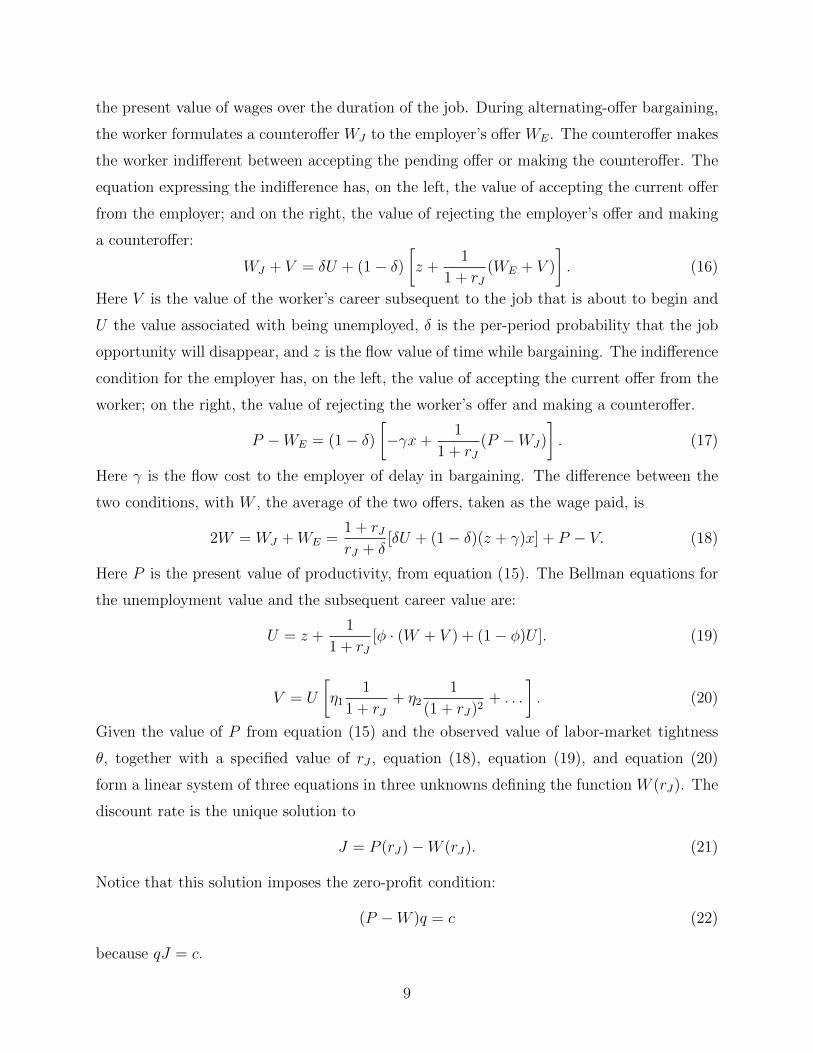
the present value of wages over the duration of the job. During alternating-offer bargaining,

the worker formulates a counteroffer WJ to the employer’s offer WE. The counteroffer makes

the worker indifferent between accepting the pending offer or making the counteroffer. The

equation expressing the indifference has, on the left, the value of accepting the current offer

from the employer; and on the right, the value of rejecting the employer’s offer and making

a counteroffer:

WJ + V = δU + (1− δ)[z +

1

1 + rJ(WE + V )

]. (16)

Here V is the value of the worker’s career subsequent to the job that is about to begin and

U the value associated with being unemployed, δ is the per-period probability that the job

opportunity will disappear, and z is the flow value of time while bargaining. The indifference

condition for the employer has, on the left, the value of accepting the current offer from the

worker; on the right, the value of rejecting the worker’s offer and making a counteroffer.

P −WE = (1− δ)[−γx+

1

1 + rJ(P −WJ)

]. (17)

Here γ is the flow cost to the employer of delay in bargaining. The difference between the

two conditions, with W , the average of the two offers, taken as the wage paid, is

2W = WJ +WE =1 + rJrJ + δ

[δU + (1− δ)(z + γ)x] + P − V. (18)

Here P is the present value of productivity, from equation (15). The Bellman equations for

the unemployment value and the subsequent career value are:

U = z +1

1 + rJ[φ · (W + V ) + (1− φ)U ]. (19)

V = U

[η1

1

1 + rJ+ η2

1

(1 + rJ)2+ . . .

]. (20)

Given the value of P from equation (15) and the observed value of labor-market tightness

θ, together with a specified value of rJ , equation (18), equation (19), and equation (20)

form a linear system of three equations in three unknowns defining the function W (rJ). The

discount rate is the unique solution to

J = P (rJ)−W (rJ). (21)

Notice that this solution imposes the zero-profit condition:

(P −W )q = c (22)

because qJ = c.

9

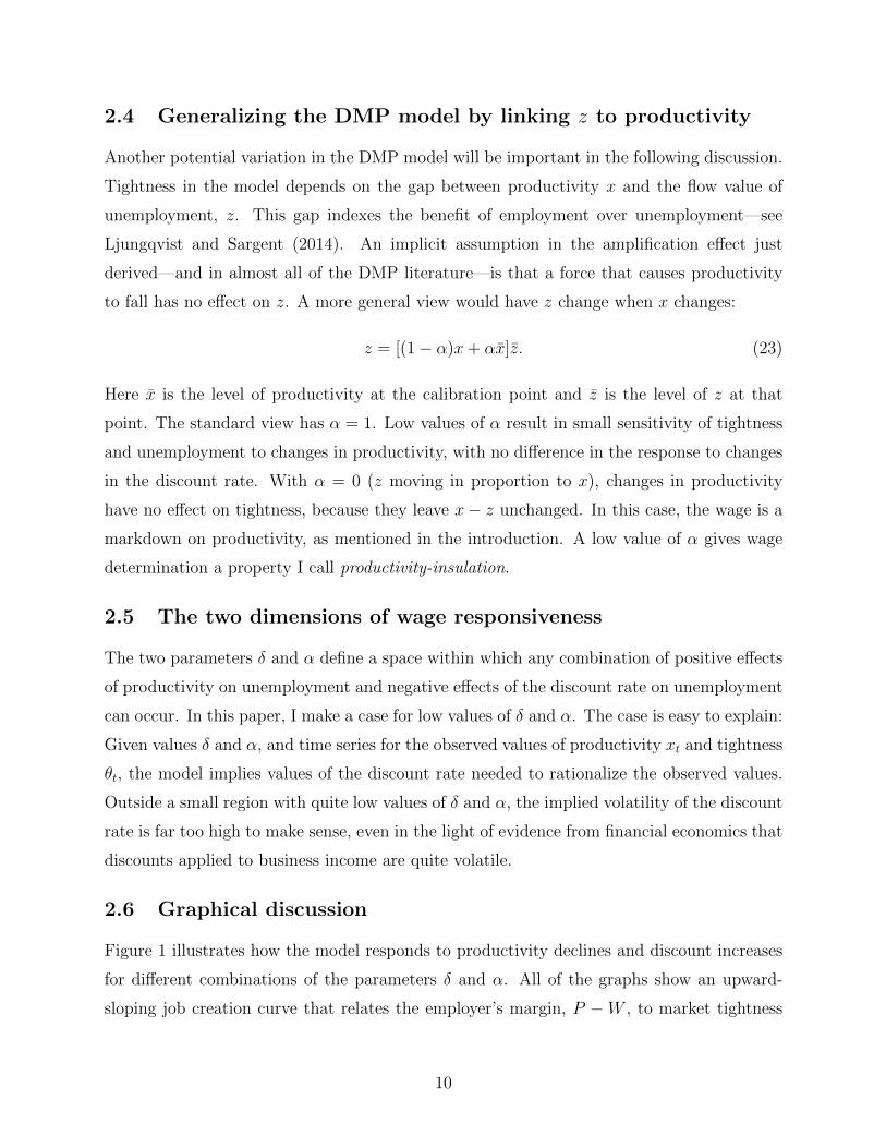
2.4 Generalizing the DMP model by linking z to productivity

Another potential variation in the DMP model will be important in the following discussion.

Tightness in the model depends on the gap between productivity x and the flow value of

unemployment, z. This gap indexes the benefit of employment over unemployment—see

Ljungqvist and Sargent (2014). An implicit assumption in the amplification effect just

derived—and in almost all of the DMP literature—is that a force that causes productivity

to fall has no effect on z. A more general view would have z change when x changes:

z = [(1− α)x+ αx]z. (23)

Here x is the level of productivity at the calibration point and z is the level of z at that

point. The standard view has α = 1. Low values of α result in small sensitivity of tightness

and unemployment to changes in productivity, with no difference in the response to changes

in the discount rate. With α = 0 (z moving in proportion to x), changes in productivity

have no effect on tightness, because they leave x− z unchanged. In this case, the wage is a

markdown on productivity, as mentioned in the introduction. A low value of α gives wage

determination a property I call productivity-insulation.

2.5 The two dimensions of wage responsiveness

The two parameters δ and α define a space within which any combination of positive effects

of productivity on unemployment and negative effects of the discount rate on unemployment

can occur. In this paper, I make a case for low values of δ and α. The case is easy to explain:

Given values δ and α, and time series for the observed values of productivity xt and tightness

θt, the model implies values of the discount rate needed to rationalize the observed values.

Outside a small region with quite low values of δ and α, the implied volatility of the discount

rate is far too high to make sense, even in the light of evidence from financial economics that

discounts applied to business income are quite volatile.

2.6 Graphical discussion

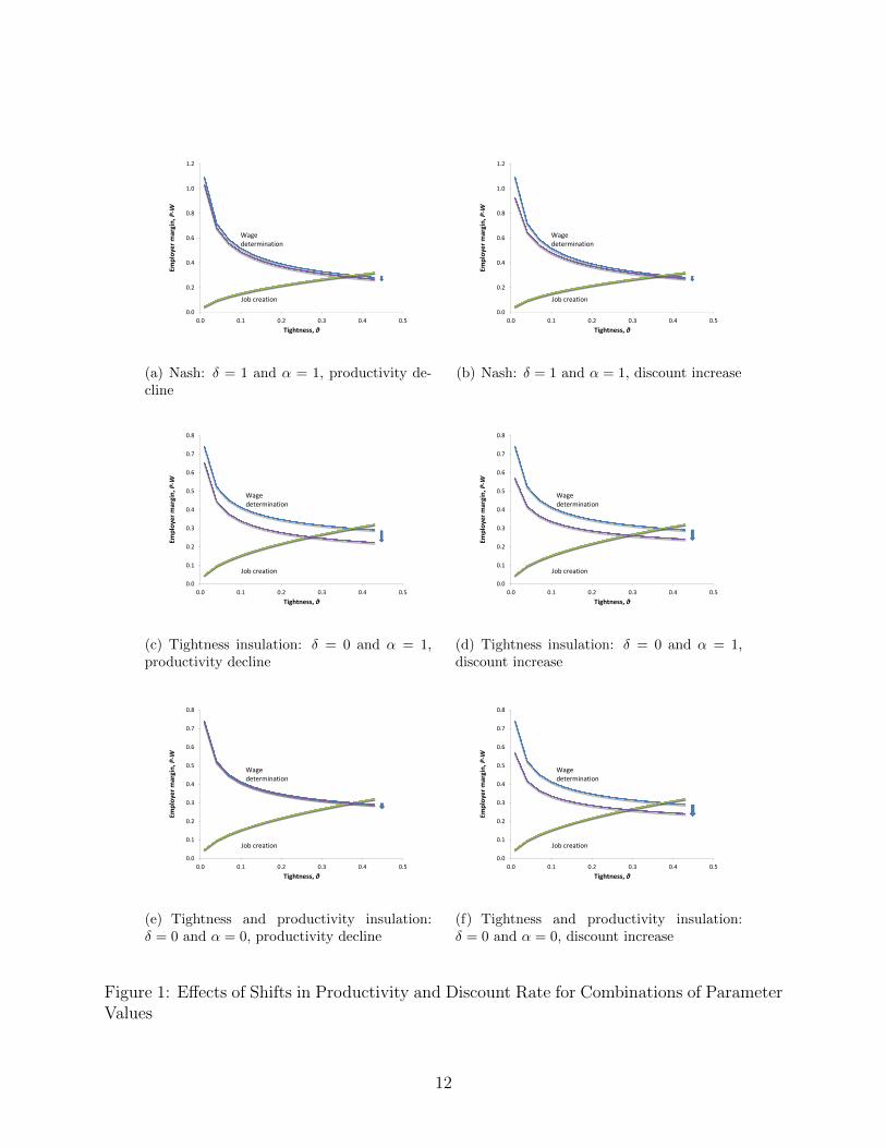
Figure 1 illustrates how the model responds to productivity declines and discount increases

for different combinations of the parameters δ and α. All of the graphs show an upward-

sloping job creation curve that relates the employer’s margin, P −W , to market tightness

10

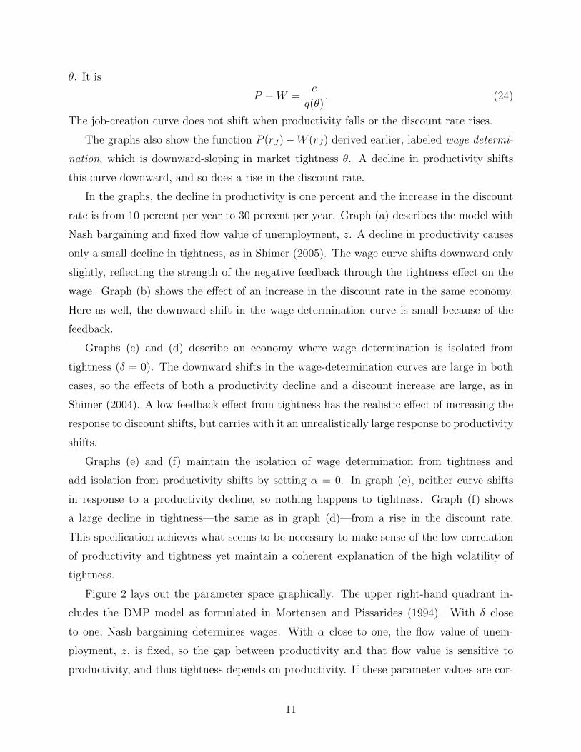
θ. It is

P −W =c

q(θ). (24)

The job-creation curve does not shift when productivity falls or the discount rate rises.

The graphs also show the function P (rJ)−W (rJ) derived earlier, labeled wage determi-

nation, which is downward-sloping in market tightness θ. A decline in productivity shifts

this curve downward, and so does a rise in the discount rate.

In the graphs, the decline in productivity is one percent and the increase in the discount

rate is from 10 percent per year to 30 percent per year. Graph (a) describes the model with

Nash bargaining and fixed flow value of unemployment, z. A decline in productivity causes

only a small decline in tightness, as in Shimer (2005). The wage curve shifts downward only

slightly, reflecting the strength of the negative feedback through the tightness effect on the

wage. Graph (b) shows the effect of an increase in the discount rate in the same economy.

Here as well, the downward shift in the wage-determination curve is small because of the

feedback.

Graphs (c) and (d) describe an economy where wage determination is isolated from

tightness (δ = 0). The downward shifts in the wage-determination curves are large in both

cases, so the effects of both a productivity decline and a discount increase are large, as in

Shimer (2004). A low feedback effect from tightness has the realistic effect of increasing the

response to discount shifts, but carries with it an unrealistically large response to productivity

shifts.

Graphs (e) and (f) maintain the isolation of wage determination from tightness and

add isolation from productivity shifts by setting α = 0. In graph (e), neither curve shifts

in response to a productivity decline, so nothing happens to tightness. Graph (f) shows

a large decline in tightness—the same as in graph (d)—from a rise in the discount rate.

This specification achieves what seems to be necessary to make sense of the low correlation

of productivity and tightness yet maintain a coherent explanation of the high volatility of

tightness.

Figure 2 lays out the parameter space graphically. The upper right-hand quadrant in-

cludes the DMP model as formulated in Mortensen and Pissarides (1994). With δ close

to one, Nash bargaining determines wages. With α close to one, the flow value of unem-

ployment, z, is fixed, so the gap between productivity and that flow value is sensitive to

productivity, and thus tightness depends on productivity. If these parameter values are cor-

11

0.0

0.2

0.4

0.6

0.8

1.0

1.2

0.0 0.1 0.2 0.3 0.4 0.5

Employer m

argin, P‐W

Tightness, θ

Job creation

Wage determination

(a) Nash: δ = 1 and α = 1, productivity de-cline

0.0

0.2

0.4

0.6

0.8

1.0

1.2

0.0 0.1 0.2 0.3 0.4 0.5

Employer m

argin, P‐W

Tightness, θ

Job creation

Wage determination

(b) Nash: δ = 1 and α = 1, discount increase

0.0

0.1

0.2

0.3

0.4

0.5

0.6

0.7

0.8

0.0 0.1 0.2 0.3 0.4 0.5

Employer m

argin, P‐W

Tightness, θ

Job creation

Wage determination

(c) Tightness insulation: δ = 0 and α = 1,productivity decline

0.0

0.1

0.2

0.3

0.4

0.5

0.6

0.7

0.8

0.0 0.1 0.2 0.3 0.4 0.5

Employer m

argin, P‐W

Tightness, θ

Job creation

Wage determination

(d) Tightness insulation: δ = 0 and α = 1,discount increase

0.0

0.1

0.2

0.3

0.4

0.5

0.6

0.7

0.8

0.0 0.1 0.2 0.3 0.4 0.5

Employer m

argin, P‐W

Tightness, θ

Job creation

Wage determination

(e) Tightness and productivity insulation:δ = 0 and α = 0, productivity decline

0.0

0.1

0.2

0.3

0.4

0.5

0.6

0.7

0.8

0.0 0.1 0.2 0.3 0.4 0.5

Employer m

argin, P‐W

Tightness, θ

Job creation

Wage determination

(f) Tightness and productivity insulation:δ = 0 and α = 0, discount increase

Figure 1: Effects of Shifts in Productivity and Discount Rate for Combinations of ParameterValues

12

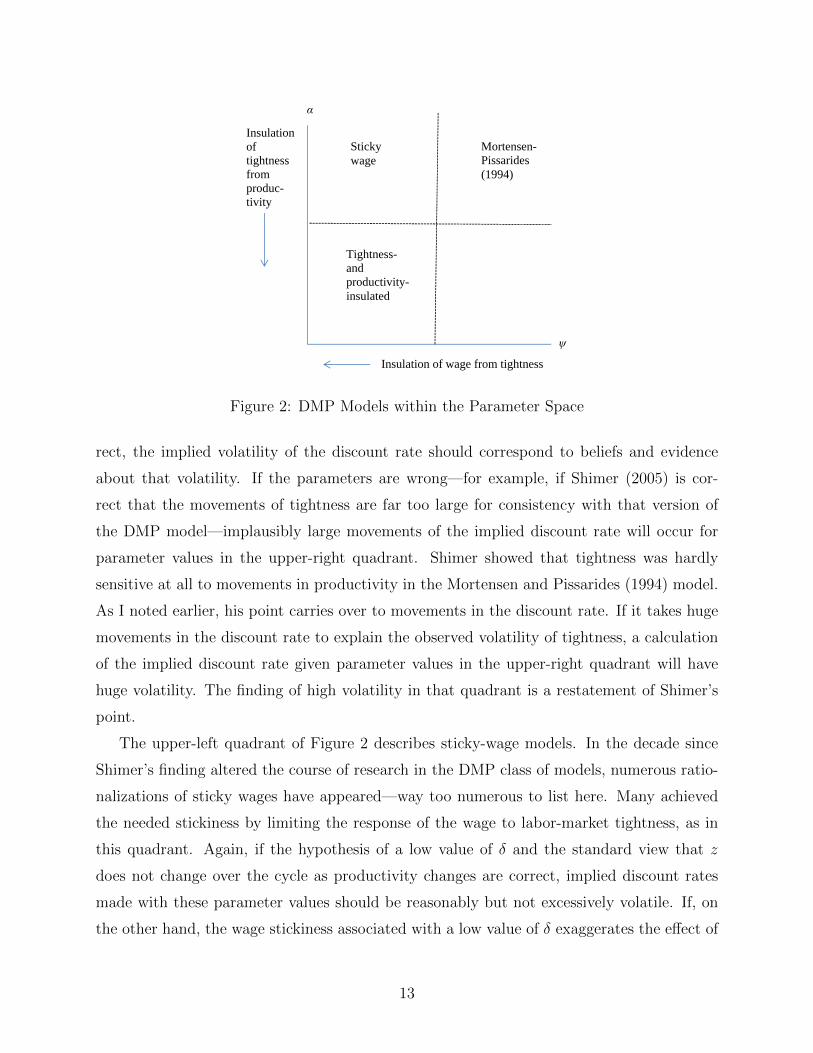
α

ψ

Insulation of tightness from produc-tivity

Insulation of wage from tightness

Mortensen-Pissarides (1994)

Sticky wage

Tightness- and productivity-insulated

Figure 2: DMP Models within the Parameter Space

rect, the implied volatility of the discount rate should correspond to beliefs and evidence

about that volatility. If the parameters are wrong—for example, if Shimer (2005) is cor-

rect that the movements of tightness are far too large for consistency with that version of

the DMP model—implausibly large movements of the implied discount rate will occur for

parameter values in the upper-right quadrant. Shimer showed that tightness was hardly

sensitive at all to movements in productivity in the Mortensen and Pissarides (1994) model.

As I noted earlier, his point carries over to movements in the discount rate. If it takes huge

movements in the discount rate to explain the observed volatility of tightness, a calculation

of the implied discount rate given parameter values in the upper-right quadrant will have

huge volatility. The finding of high volatility in that quadrant is a restatement of Shimer’s

point.

The upper-left quadrant of Figure 2 describes sticky-wage models. In the decade since

Shimer’s finding altered the course of research in the DMP class of models, numerous ratio-

nalizations of sticky wages have appeared—way too numerous to list here. Many achieved

the needed stickiness by limiting the response of the wage to labor-market tightness, as in

this quadrant. Again, if the hypothesis of a low value of δ and the standard view that z

does not change over the cycle as productivity changes are correct, implied discount rates

made with these parameter values should be reasonably but not excessively volatile. If, on

the other hand, the wage stickiness associated with a low value of δ exaggerates the effect of

13

productivity on tightness, then the implied discount rate will be unreasonably volatile be-

cause it will move to offset the exaggerated effects of productivity. Thus a finding of a high

volatility of the implied discount rate will point away from a standard sticky-wage model.

Finally, the lower-left quadrant of Figure 2 contains DMP models that respond weakly to

productivity movements but are reasonably sensitive to movements in discount rates. These

models are sensitive to the gap x− z that is the basic source of the response of tightness to

productivity movements, but the gap hardly changes when x changes because z changes in

parallel. If these parameter values hold, the implied time series for the discount rate will be

correct, so its volatility will be in line with evidence and beliefs. On the other hand, if, for

example, a low value of α understates the role of productivity movements on tightness, the

implied discount rate will make up for the neglected influence of productivity and will have

an implausible volatility.

3 Measuring the Implied Volatility of the Discount

Rate

3.1 Measuring the job value

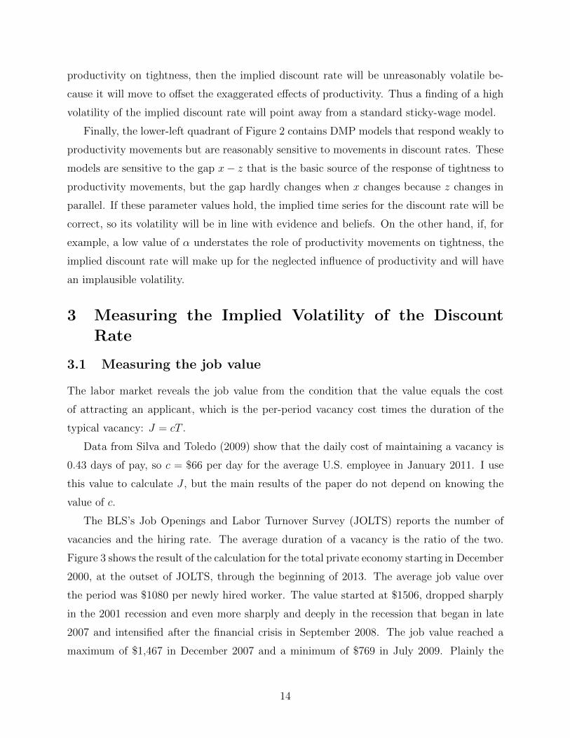
The labor market reveals the job value from the condition that the value equals the cost

of attracting an applicant, which is the per-period vacancy cost times the duration of the

typical vacancy: J = cT .

Data from Silva and Toledo (2009) show that the daily cost of maintaining a vacancy is

0.43 days of pay, so c = $66 per day for the average U.S. employee in January 2011. I use

this value to calculate J , but the main results of the paper do not depend on knowing the

value of c.

The BLS’s Job Openings and Labor Turnover Survey (JOLTS) reports the number of

vacancies and the hiring rate. The average duration of a vacancy is the ratio of the two.

Figure 3 shows the result of the calculation for the total private economy starting in December

2000, at the outset of JOLTS, through the beginning of 2013. The average job value over

the period was $1080 per newly hired worker. The value started at $1506, dropped sharply

in the 2001 recession and even more sharply and deeply in the recession that began in late

2007 and intensified after the financial crisis in September 2008. The job value reached a

maximum of $1,467 in December 2007 and a minimum of $769 in July 2009. Plainly the

14

0

200

400

600

800

1000

1200

1400

1600

2000 2002 2004 2006 2008 2010 2012

Figure 3: Aggregate Job Value, 2001 through 2013

incentive to create jobs fell substantially over that interval. Hall and Schulhofer-Wohl (2013)

compare the hiring flows from JOLTS to the total flow into new jobs from unemployment,

those out of the labor force, and job-changers. The level of the flows is higher in the CPS

data and the decline in the recession was somewhat larger as well. None of the results in

this paper would be affected by the use of the CPS hiring flow in place of the JOLTS flow.

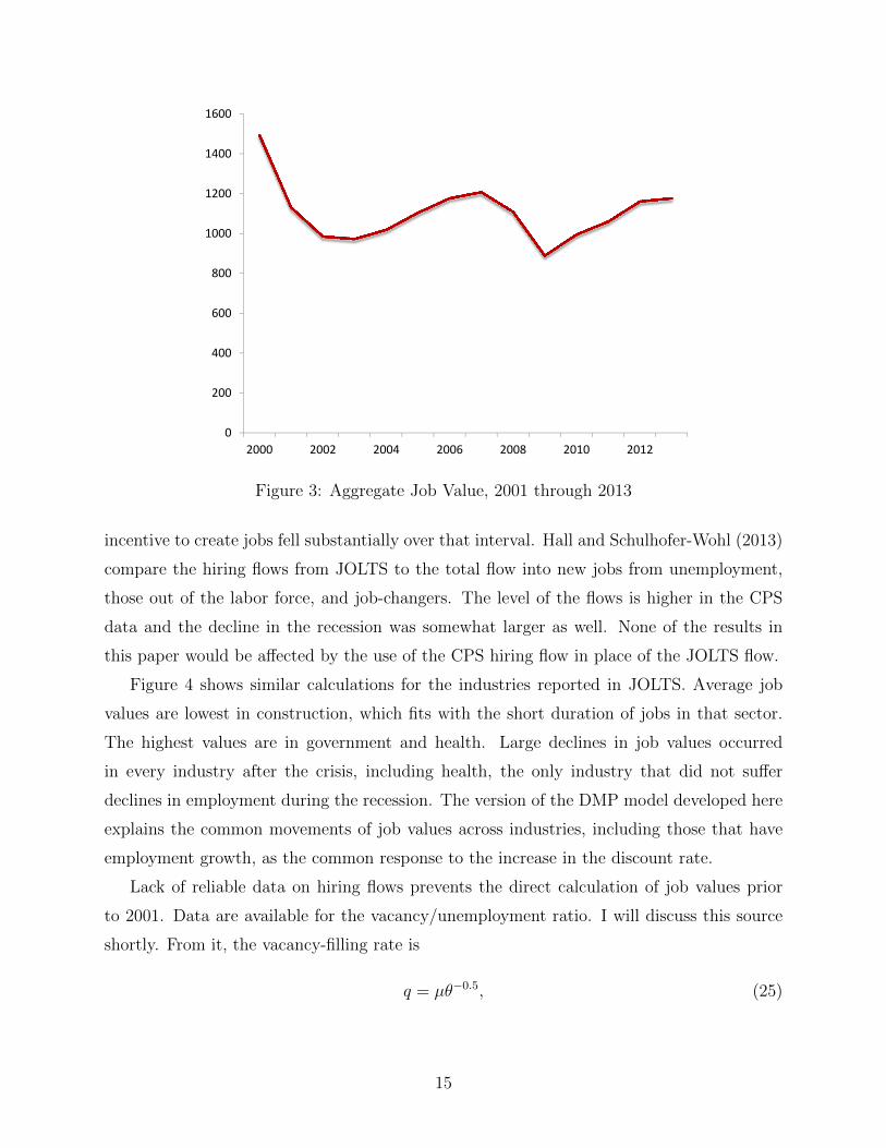
Figure 4 shows similar calculations for the industries reported in JOLTS. Average job

values are lowest in construction, which fits with the short duration of jobs in that sector.

The highest values are in government and health. Large declines in job values occurred

in every industry after the crisis, including health, the only industry that did not suffer

declines in employment during the recession. The version of the DMP model developed here

explains the common movements of job values across industries, including those that have

employment growth, as the common response to the increase in the discount rate.

Lack of reliable data on hiring flows prevents the direct calculation of job values prior

to 2001. Data are available for the vacancy/unemployment ratio. I will discuss this source

shortly. From it, the vacancy-filling rate is

q = µθ−0.5, (25)

15

0

500

1000

1500

2000

2500

2001 2003 2005 2007 2009 2011 2013

Job value, dollars

Accomodation

Construction

Education

Entertainment

Health

Manufacturing

Prof services

Retail

State and Local

Wholesale,transport,utilities

Figure 4: Job Values by Industry, 2001 through 2013

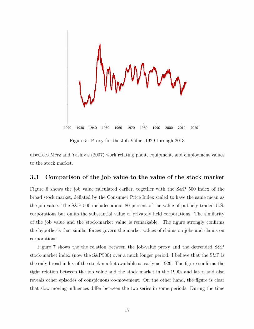
using the years 2001 through 2007 to measure matching efficiency µ (efficiency dropped

sharply beginning in 2008). Figure 5 shows the job-value proxy. It is a completely reliable

cyclical indicator, negatively correlated with unemployment.

3.2 The relation between the job value and the stock market

Kuehn, Petrosky-Nadeau and Zhang (2013) show that, in a model without capital, the

return to holding a firm’s stock is the same as the return to hiring a worker. In levels, the

same proposition is that the value of the firm in the stock market is the value of what it

owns. Under a policy of paying out earnings as dividends, rather than holding securities or

borrowing, the firm without capital owns only one asset, its relationships with its workers.

The stock market reveals the job value of workers (the amount c/q) plus any other costs

the firm incurred with the expectation that they would be earned back from the future

difference between productivity and wage, x− w. Of course, in reality firms also own plant

and equipment. One could imagine trying to recover the job value by subtracting the value

of plant and equipment and other assets from the total stock-market value. Hall (2001)

suggests that the results would not make sense. In some eras, the stock-market value falls

far short of the value of plant and equipment alone, while in others, the value is far above that

benchmark, much further than any reasonable job value could account for. The appendix

16

0

500

1000

1500

2000

2500

1920 1930 1940 1950 1960 1970 1980 1990 2000 2010 2020

Figure 5: Proxy for the Job Value, 1929 through 2013

discusses Merz and Yashiv’s (2007) work relating plant, equipment, and employment values

to the stock market.

3.3 Comparison of the job value to the value of the stock market

Figure 6 shows the job value calculated earlier, together with the S&P 500 index of the

broad stock market, deflated by the Consumer Price Index scaled to have the same mean as

the job value. The S&P 500 includes about 80 percent of the value of publicly traded U.S.

corporations but omits the substantial value of privately held corporations. The similarity

of the job value and the stock-market value is remarkable. The figure strongly confirms

the hypothesis that similar forces govern the market values of claims on jobs and claims on

corporations.

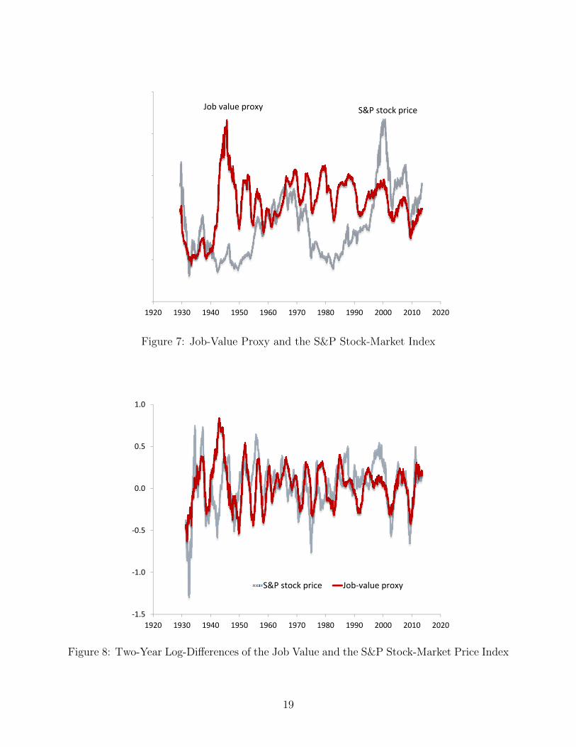
Figure 7 shows the the relation between the job-value proxy and the detrended S&P

stock-market index (now the S&P500) over a much longer period. I believe that the S&P is

the only broad index of the stock market available as early as 1929. The figure confirms the

tight relation between the job value and the stock market in the 1990s and later, and also

reveals other episodes of conspicuous co-movement. On the other hand, the figure is clear

that slow-moving influences differ between the two series in some periods. During the time

17

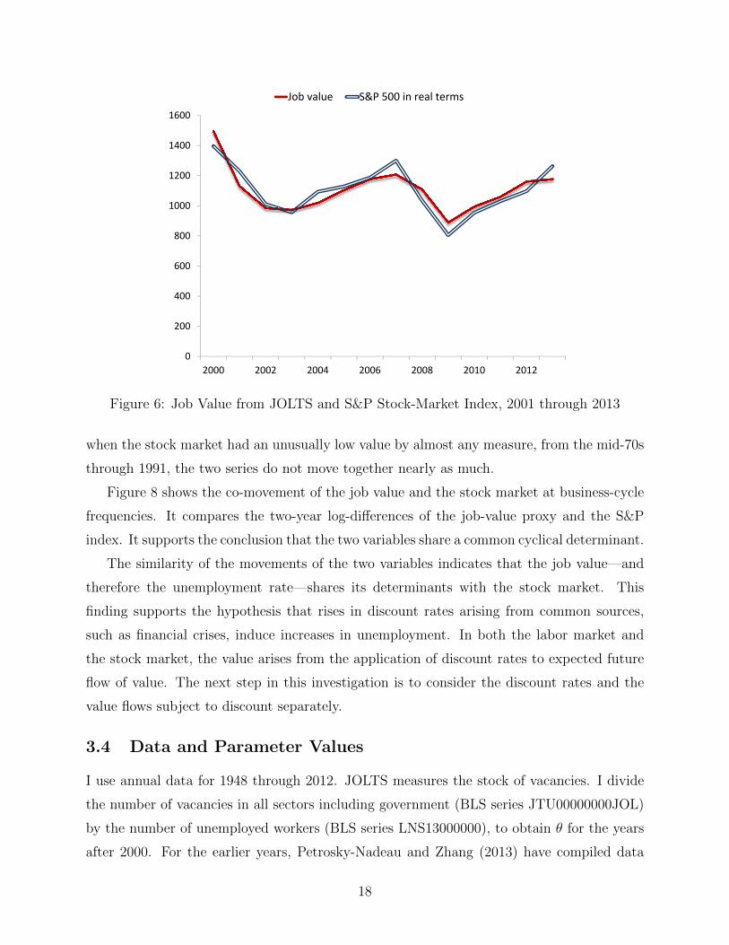
0

200

400

600

800

1000

1200

1400

1600

2000 2002 2004 2006 2008 2010 2012

Job value S&P 500 in real terms

Figure 6: Job Value from JOLTS and S&P Stock-Market Index, 2001 through 2013

when the stock market had an unusually low value by almost any measure, from the mid-70s

through 1991, the two series do not move together nearly as much.

Figure 8 shows the co-movement of the job value and the stock market at business-cycle

frequencies. It compares the two-year log-differences of the job-value proxy and the S&P

index. It supports the conclusion that the two variables share a common cyclical determinant.

The similarity of the movements of the two variables indicates that the job value—and

therefore the unemployment rate—shares its determinants with the stock market. This

finding supports the hypothesis that rises in discount rates arising from common sources,

such as financial crises, induce increases in unemployment. In both the labor market and

the stock market, the value arises from the application of discount rates to expected future

flow of value. The next step in this investigation is to consider the discount rates and the

value flows subject to discount separately.

3.4 Data and Parameter Values

I use annual data for 1948 through 2012. JOLTS measures the stock of vacancies. I divide

the number of vacancies in all sectors including government (BLS series JTU00000000JOL)

by the number of unemployed workers (BLS series LNS13000000), to obtain θ for the years

after 2000. For the earlier years, Petrosky-Nadeau and Zhang (2013) have compiled data

18

0

500

1000

1500

2000

2500

1920 1930 1940 1950 1960 1970 1980 1990 2000 2010 2020

S&P stock priceJob value proxy

Figure 7: Job-Value Proxy and the S&P Stock-Market Index

‐1.5

‐1.0

‐0.5

0.0

0.5

1.0

1920 1930 1940 1950 1960 1970 1980 1990 2000 2010 2020

S&P stock price Job‐value proxy

Figure 8: Two-Year Log-Differences of the Job Value and the S&P Stock-Market Price Index

19

0.00

0.10

0.20

0.30

0.40

0.50

0.60

0.70

0.80

0.90

1.00

1948 1953 1958 1963 1968 1973 1978 1983 1988 1993 1998 2003 2008

Figure 9: The Vacancy/Unemployment Ratio, θ, 1948 through 2012

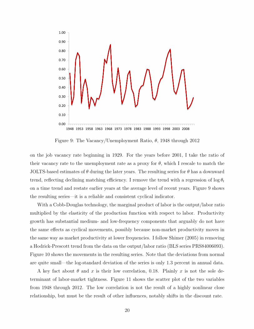
on the job vacancy rate beginning in 1929. For the years before 2001, I take the ratio of

their vacancy rate to the unemployment rate as a proxy for θ, which I rescale to match the

JOLTS-based estimates of θ during the later years. The resulting series for θ has a downward

trend, reflecting declining matching efficiency. I remove the trend with a regression of log θt

on a time trend and restate earlier years at the average level of recent years. Figure 9 shows

the resulting series—it is a reliable and consistent cyclical indicator.

With a Cobb-Douglas technology, the marginal product of labor is the output/labor ratio

multiplied by the elasticity of the production function with respect to labor. Productivity

growth has substantial medium- and low-frequency components that arguably do not have

the same effects as cyclical movements, possibly because non-market productivity moves in

the same way as market productivity at lower frequencies. I follow Shimer (2005) in removing

a Hodrick-Prescott trend from the data on the output/labor ratio (BLS series PRS84006093).

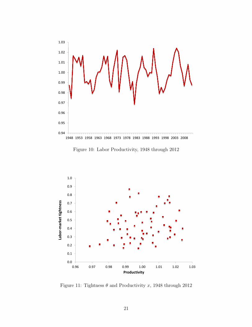
Figure 10 shows the movements in the resulting series. Note that the deviations from normal

are quite small—the log-standard deviation of the series is only 1.3 percent in annual data.

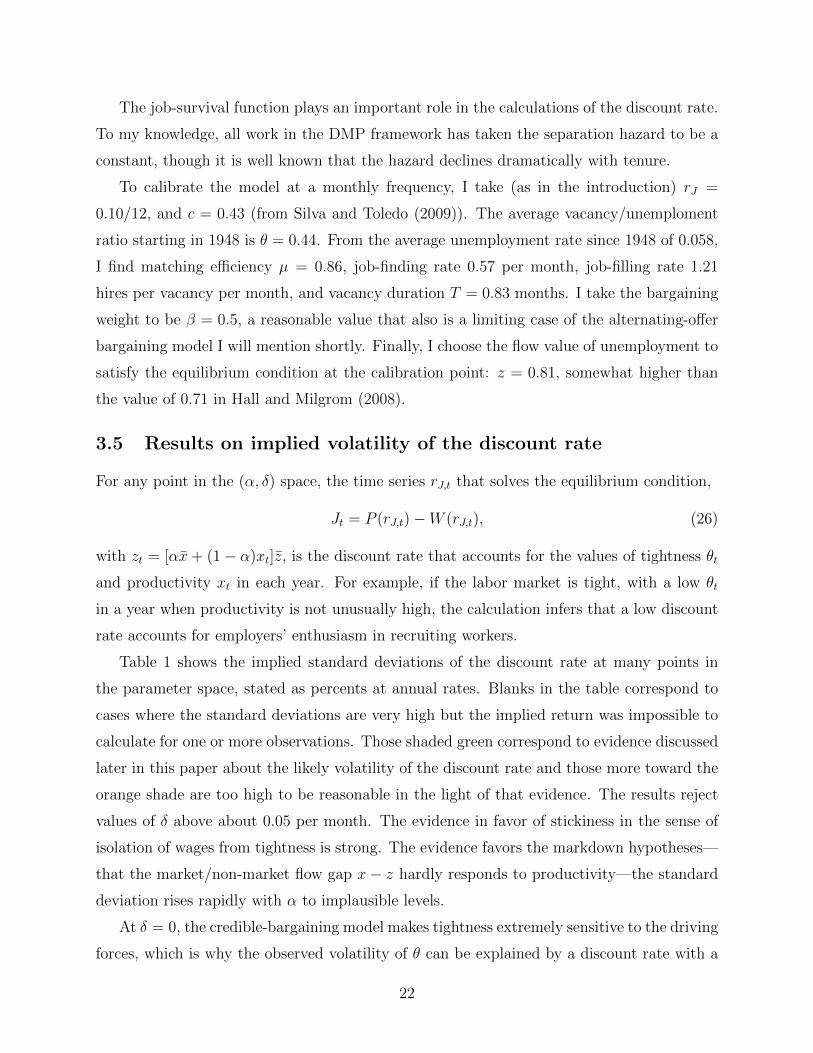
A key fact about θ and x is their low correlation, 0.18. Plainly x is not the sole de-

terminant of labor-market tightness. Figure 11 shows the scatter plot of the two variables

from 1948 through 2012. The low correlation is not the result of a highly nonlinear close

relationship, but must be the result of other influences, notably shifts in the discount rate.

20

0.94

0.95

0.96

0.97

0.98

0.99

1.00

1.01

1.02

1.03

1948 1953 1958 1963 1968 1973 1978 1983 1988 1993 1998 2003 2008

Figure 10: Labor Productivity, 1948 through 2012

0.0

0.1

0.2

0.3

0.4

0.5

0.6

0.7

0.8

0.9

1.0

0.96 0.97 0.98 0.99 1.00 1.01 1.02 1.03

Labo

r‐market tightne

ss

Productivity

Figure 11: Tightness θ and Productivity x, 1948 through 2012

21

The job-survival function plays an important role in the calculations of the discount rate.

To my knowledge, all work in the DMP framework has taken the separation hazard to be a

constant, though it is well known that the hazard declines dramatically with tenure.

To calibrate the model at a monthly frequency, I take (as in the introduction) rJ =

0.10/12, and c = 0.43 (from Silva and Toledo (2009)). The average vacancy/unemploment

ratio starting in 1948 is θ = 0.44. From the average unemployment rate since 1948 of 0.058,

I find matching efficiency µ = 0.86, job-finding rate 0.57 per month, job-filling rate 1.21

hires per vacancy per month, and vacancy duration T = 0.83 months. I take the bargaining

weight to be β = 0.5, a reasonable value that also is a limiting case of the alternating-offer

bargaining model I will mention shortly. Finally, I choose the flow value of unemployment to

satisfy the equilibrium condition at the calibration point: z = 0.81, somewhat higher than

the value of 0.71 in Hall and Milgrom (2008).

3.5 Results on implied volatility of the discount rate

For any point in the (α, δ) space, the time series rJ,t that solves the equilibrium condition,

Jt = P (rJ,t)−W (rJ,t), (26)

with zt = [αx+ (1− α)xt]z, is the discount rate that accounts for the values of tightness θt

and productivity xt in each year. For example, if the labor market is tight, with a low θt

in a year when productivity is not unusually high, the calculation infers that a low discount

rate accounts for employers’ enthusiasm in recruiting workers.

Table 1 shows the implied standard deviations of the discount rate at many points in

the parameter space, stated as percents at annual rates. Blanks in the table correspond to

cases where the standard deviations are very high but the implied return was impossible to

calculate for one or more observations. Those shaded green correspond to evidence discussed

later in this paper about the likely volatility of the discount rate and those more toward the

orange shade are too high to be reasonable in the light of that evidence. The results reject

values of δ above about 0.05 per month. The evidence in favor of stickiness in the sense of

isolation of wages from tightness is strong. The evidence favors the markdown hypotheses—

that the market/non-market flow gap x− z hardly responds to productivity—the standard

deviation rises rapidly with α to implausible levels.

At δ = 0, the credible-bargaining model makes tightness extremely sensitive to the driving

forces, which is why the observed volatility of θ can be explained by a discount rate with a

22

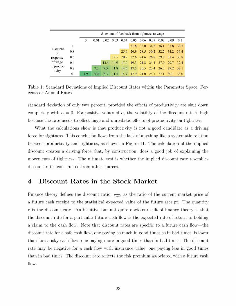
0 0.01 0.02 0.03 0.04 0.05 0.06 0.07 0.08 0.09 0.11 31.8 33.0 34.5 36.1 37.8 39.7

0.8 25.6 26.9 28.5 30.2 32.2 34.2 36.40.6 19.5 20.9 22.6 24.6 26.8 29.0 31.4 33.80.4 13.4 14.9 17.0 19.3 21.8 24.4 27.0 29.7 32.40.2 7.3 9.3 11.8 14.6 17.5 20.5 23.4 26.3 29.2 32.10 1.9 5.0 8.3 11.5 14.7 17.9 21.0 24.1 27.1 30.1 33.0

δ : extent of feedback from tightness to wage

α: extent of

response of wage

to produc-tivity

Table 1: Standard Deviations of Implied Discount Rates within the Parameter Space, Per-cents at Annual Rates

standard deviation of only two percent, provided the effects of productivity are shut down

completely with α = 0. For positive values of α, the volatility of the discount rate is high

because the rate needs to offset huge and unrealistic effects of productivity on tightness.

What the calculations show is that productivity is not a good candidate as a driving

force for tightness. This conclusion flows from the lack of anything like a systematic relation

between productivity and tightness, as shown in Figure 11. The calculation of the implied

discount creates a driving force that, by construction, does a good job of explaining the

movements of tightness. The ultimate test is whether the implied discount rate resembles

discount rates constructed from other sources.

4 Discount Rates in the Stock Market

Finance theory defines the discount ratio, 11+r

, as the ratio of the current market price of

a future cash receipt to the statistical expected value of the future receipt. The quantity

r is the discount rate. An intuitive but not quite obvious result of finance theory is that

the discount rate for a particular future cash flow is the expected rate of return to holding

a claim to the cash flow. Note that discount rates are specific to a future cash flow—the

discount rate for a safe cash flow, one paying as much in good times as in bad times, is lower

than for a risky cash flow, one paying more in good times than in bad times. The discount

rate may be negative for a cash flow with insurance value, one paying less in good times

than in bad times. The discount rate reflects the risk premium associated with a future cash

flow.

23

‐5

0

5

10

15

20

25

30

35

40

1950 1955 1960 1965 1970 1975 1980 1985 1990 1995 2000 2005 2010

Figure 12: Econometric Measure of the Discount Rate for the S&P Stock-Price Index

This paper does not explain why risky flows receive higher discounts in recessions (but see

Bianchi, Ilut and Schneider (2012) for a new stab at an explanation). Rather, it documents

that fact by extracting the discount rates implicit in the stock market.

4.1 The discount rate for the S&P stock-price index

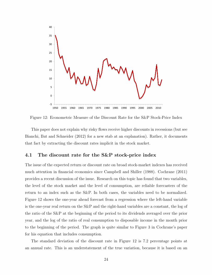
The issue of the expected return or discount rate on broad stock-market indexes has received

much attention in financial economics since Campbell and Shiller (1988). Cochrane (2011)

provides a recent discussion of the issue. Research on this topic has found that two variables,

the level of the stock market and the level of consumption, are reliable forecasters of the

return to an index such as the S&P. In both cases, the variables need to be normalized.

Figure 12 shows the one-year ahead forecast from a regression where the left-hand variable

is the one-year real return on the S&P and the right-hand variables are a constant, the log of

the ratio of the S&P at the beginning of the period to its dividends averaged over the prior

year, and the log of the ratio of real consumption to disposable income in the month prior

to the beginning of the period. The graph is quite similar to Figure 3 in Cochrane’s paper

for his equation that includes consumption.

The standard deviation of the discount rate in Figure 12 is 7.2 percentage points at

an annual rate. This is an understatement of the true variation, because it is based on an

24

econometric forecast using only a subset of the information available at the time the forecasts

would have been made.

Another source of evidence on the volatility of expected returns in the stock market

comes from the Livingston survey, which has been recording professional forecasts of the

S&P stock-price index since 1952. The standard deviation of the one-year forward expected

change in the index in real terms plus the current dividend yield is 5.8 percent.

So far I have considered the volatility of the expected return in the stock market for an

investment held for one year. The future cash flow subject to discount is the value from

selling the stock in a year, inclusive of the dividends earned over the year reinvested in the

same stock. Most of the risk arises from fluctuations in the price of the stock rather than

from the value of the dividends, so the risk under consideration in calculating the expected

return arises from all future time periods, not just from the year of the calculation. The

stock market looks much further into the future than does a firm evaluating the benefit from

hiring a worker, as most jobs last only a few years. One way to deal with that issue is to

study the valuation of claims to dividends accruing over near-term intervals. Such claims

are called “dividend strips” and trade in active markets. Because dividends are close to

smoothed earnings, values of dividend strips reveal valuations of near-term earnings. Jules

van Binsbergen, Brandt and Koijen (2012) and van Binsbergen, Hueskes, Koijen and Vrugt

(2013) pioneered the study of the valuation of dividend strips, with the important conclusion

that the volatility of discount rates for near-term dividends is comparable to the volatility

of the discount rate for the entire return from the stock market over similar durations.

These authors study two bodies of data on dividend strips. The first infers the prices

from traded options. Buying a put and selling a call with the same strike price and maturity

gives the holder the strike price less the stock price with certainty at maturity. Holding

the stock as well means that the only consequence of the overall position is to receive the

intervening dividends and pay the riskless interest rate on the amount of the strike price.

The second source of data comes from the dividend futures market. The latter provides data

for about the last decade, whereas data from options markets are available starting in 1996.

Jules van Binsbergen et al. (2012) published the options-based dividend strip data on the

AER website, for six-month periods up to two years in the future.

The market discount rate for dividends payable in 13 through 24 months is

rt =Et∑24

τ=13 dt+τpt

− 1, (27)

25

where dt is the dividend paid in month t and pt is the market price in month t of the claim to

future dividends inferred from options prices and the stock price. Measuring the conditional

expectation of future dividends in the numerator is in principle challenging, but seems not to

matter much in this case. I have experimented with discount rates for two polar extremes.

First is a naive forecast, taking the expected value to be the same as the sum of the 6

most recently observed monthly dividends as of month t. The second is a perfect-foresight

forecast, the realized value of dividends 13 through 24 months in the future. The discount

rates are very similar. Here I use the average of the two series.

The main point of van Binsbergen et al. (2012) and van Binsbergen et al. (2013) is

that the discounts (expected returns) embodied in the prices of near-future dividend strips

are remarkably volatile. Many of the explanations of the volatility of expected returns in

the stock market itself emphasize longer-run influences and imply low volatility of near-

term discounts, but the fact is that near-term discount volatility is about as high as overall

discount volatility. In the earlier years, some of the volatility seems to arise from pricing

errors or noise in the data. For example, in February 2001, the strip sold for $9.37 at a time

when the current dividend was $16.07 and the strip ultimately paid $15.87. The spike in

late 2001 occurred at the time of 9/11 and may be genuine. No similarly suspicious spikes

appear in the later years.

Over the period when these authors have compiled the needed options price, from 1996

through 2009, the standard deviation of the market discount rate on S&P500 dividends to

be received 13 to 24 months in the future, stated at an annual rate in real terms, is 10.1

percent. The standard deviations of the discount rate for the stock market over the same

period are 5.4 percent for the econometric version of the return forecast and 6.2 percent for

the return based on the Livingston survey.

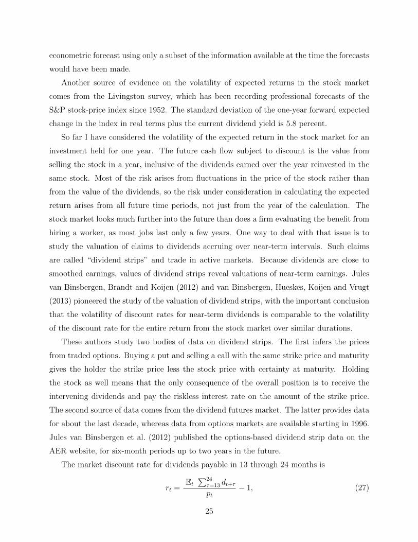
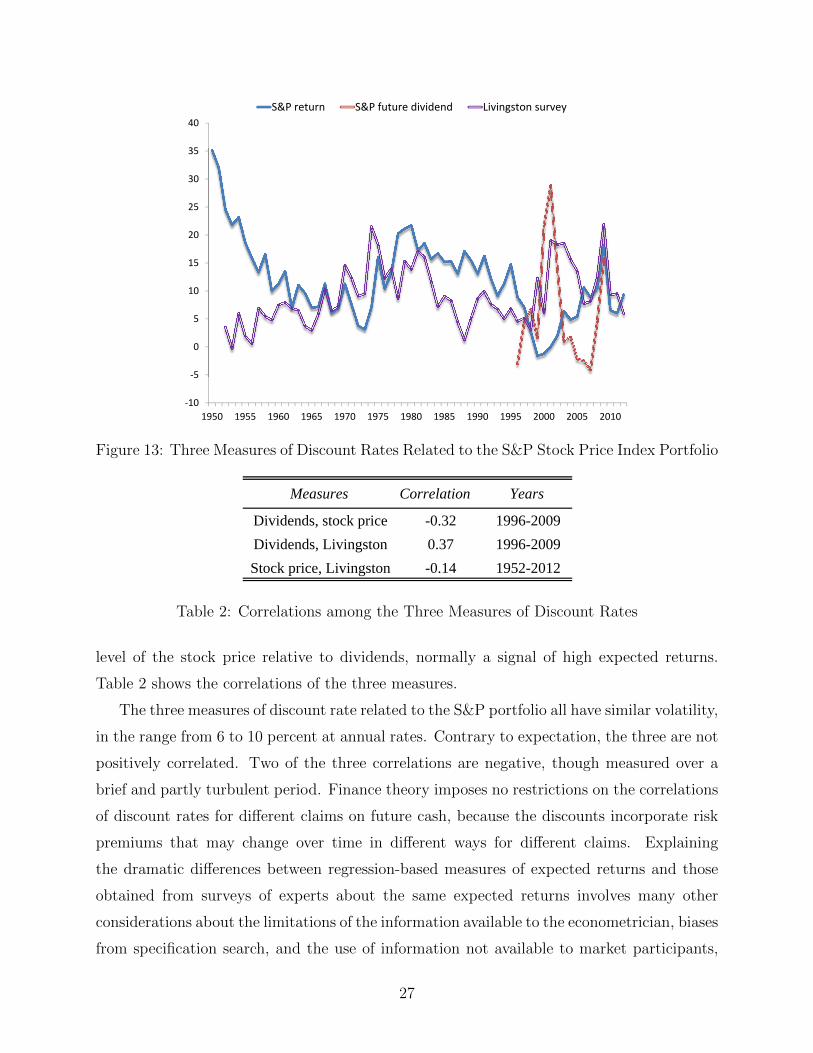
Figure 13 shows the three series for the discount rates implicit in the S&P stock price

and in the prices of dividend strips for that portfolio. On some points, the three series

agree, notably on the spike in the discount rate in 2009 after the financial crisis. In 2001, the

Livingston forecasters and the strips market revealed a comparable spike, but the econometric

forecast disagreed completely—high values of the stock market and consumption suggested

a low expected return. From 1950 to 1960, the reverse occurred. The Livingston panel had

low expectations of a rising price, whereas the econometric forecast responded to the low

26

‐10

‐5

0

5

10

15

20

25

30

35

40

1950 1955 1960 1965 1970 1975 1980 1985 1990 1995 2000 2005 2010

S&P return S&P future dividend Livingston survey

Figure 13: Three Measures of Discount Rates Related to the S&P Stock Price Index Portfolio

Measures Correlation Years

Dividends, stock price -0.32 1996-2009

Dividends, Livingston 0.37 1996-2009

Stock price, Livingston -0.14 1952-2012

Table 2: Correlations among the Three Measures of Discount Rates

level of the stock price relative to dividends, normally a signal of high expected returns.

Table 2 shows the correlations of the three measures.

The three measures of discount rate related to the S&P portfolio all have similar volatility,

in the range from 6 to 10 percent at annual rates. Contrary to expectation, the three are not

positively correlated. Two of the three correlations are negative, though measured over a

brief and partly turbulent period. Finance theory imposes no restrictions on the correlations

of discount rates for different claims on future cash, because the discounts incorporate risk

premiums that may change over time in different ways for different claims. Explaining

the dramatic differences between regression-based measures of expected returns and those

obtained from surveys of experts about the same expected returns involves many other

considerations about the limitations of the information available to the econometrician, biases

from specification search, and the use of information not available to market participants,

27

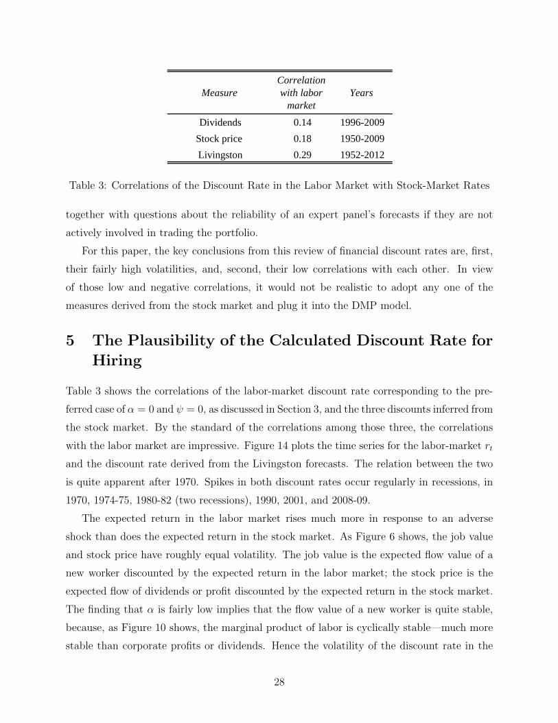
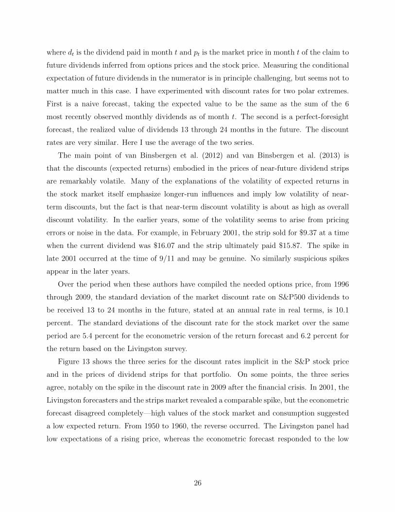
MeasureCorrelation with labor

marketYears

Dividends 0.14 1996-2009

Stock price 0.18 1950-2009

Livingston 0.29 1952-2012

Table 3: Correlations of the Discount Rate in the Labor Market with Stock-Market Rates

together with questions about the reliability of an expert panel’s forecasts if they are not

actively involved in trading the portfolio.

For this paper, the key conclusions from this review of financial discount rates are, first,

their fairly high volatilities, and, second, their low correlations with each other. In view

of those low and negative correlations, it would not be realistic to adopt any one of the

measures derived from the stock market and plug it into the DMP model.

5 The Plausibility of the Calculated Discount Rate for

Hiring

Table 3 shows the correlations of the labor-market discount rate corresponding to the pre-

ferred case of α = 0 and ψ = 0, as discussed in Section 3, and the three discounts inferred from

the stock market. By the standard of the correlations among those three, the correlations

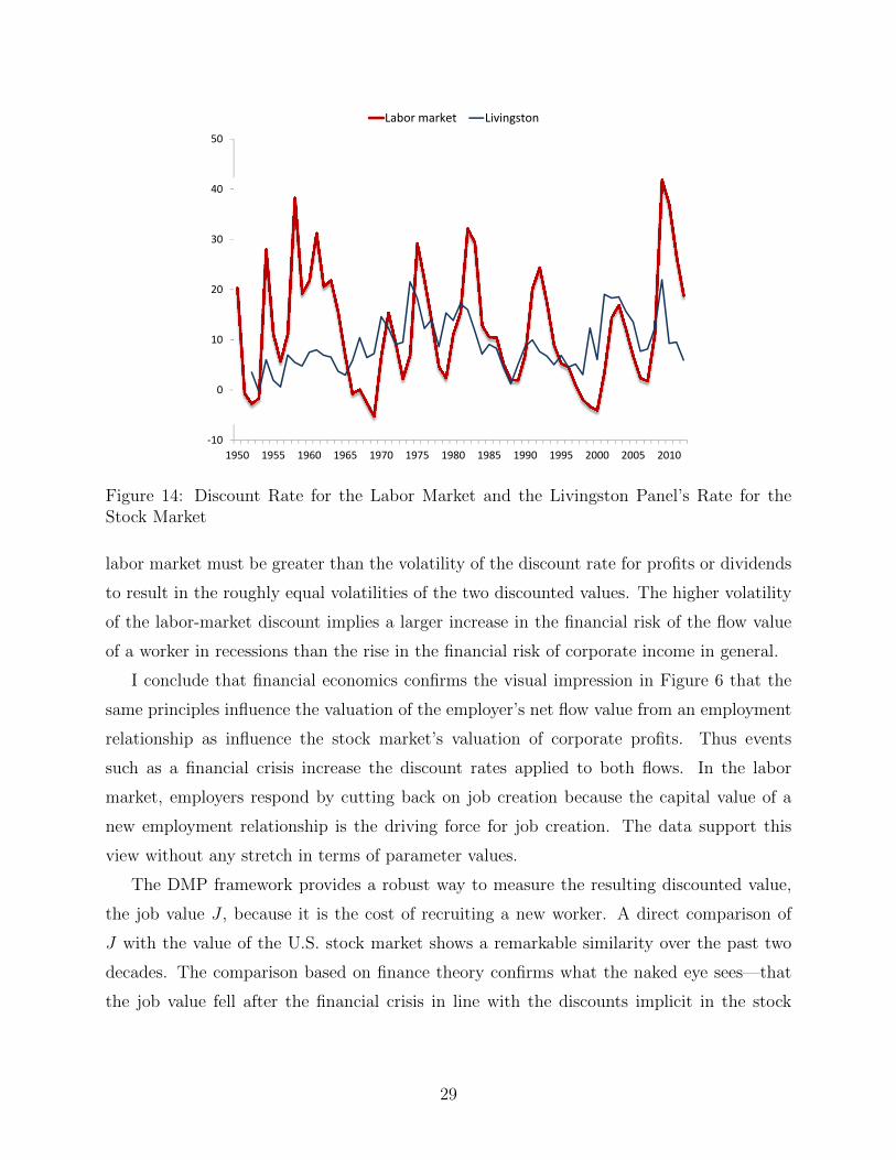
with the labor market are impressive. Figure 14 plots the time series for the labor-market rt

and the discount rate derived from the Livingston forecasts. The relation between the two

is quite apparent after 1970. Spikes in both discount rates occur regularly in recessions, in

1970, 1974-75, 1980-82 (two recessions), 1990, 2001, and 2008-09.

The expected return in the labor market rises much more in response to an adverse

shock than does the expected return in the stock market. As Figure 6 shows, the job value

and stock price have roughly equal volatility. The job value is the expected flow value of a

new worker discounted by the expected return in the labor market; the stock price is the

expected flow of dividends or profit discounted by the expected return in the stock market.

The finding that α is fairly low implies that the flow value of a new worker is quite stable,

because, as Figure 10 shows, the marginal product of labor is cyclically stable—much more

stable than corporate profits or dividends. Hence the volatility of the discount rate in the

28

‐10

0

10

20

30

40

50

1950 1955 1960 1965 1970 1975 1980 1985 1990 1995 2000 2005 2010

Labor market Livingston

Figure 14: Discount Rate for the Labor Market and the Livingston Panel’s Rate for theStock Market

labor market must be greater than the volatility of the discount rate for profits or dividends

to result in the roughly equal volatilities of the two discounted values. The higher volatility

of the labor-market discount implies a larger increase in the financial risk of the flow value

of a worker in recessions than the rise in the financial risk of corporate income in general.

I conclude that financial economics confirms the visual impression in Figure 6 that the

same principles influence the valuation of the employer’s net flow value from an employment

relationship as influence the stock market’s valuation of corporate profits. Thus events

such as a financial crisis increase the discount rates applied to both flows. In the labor

market, employers respond by cutting back on job creation because the capital value of a

new employment relationship is the driving force for job creation. The data support this

view without any stretch in terms of parameter values.

The DMP framework provides a robust way to measure the resulting discounted value,

the job value J , because it is the cost of recruiting a new worker. A direct comparison of

J with the value of the U.S. stock market shows a remarkable similarity over the past two

decades. The comparison based on finance theory confirms what the naked eye sees—that

the job value fell after the financial crisis in line with the discounts implicit in the stock

29

market. To put it differently, a large increase in the equity premium appears to have applied

to the net benefit of hiring a new worker as well as to the stock market.

6 Evidence on the Relationship between Productivity

and the Flow Value of Unemployment

Chodorow-Reich and Karabarbounis (2013) study the movements of the flow value of unem-

ployment, z, or, as they term the concept, the opportunity cost of work. I believe that theirs

is the only contribution on this subject. They conclude that z moves at cyclical frequencies

in proportion to productivity. They start from an expression for z in Hall and Milgrom

(2008) with two components. The first is the level of unemployment-conditioned benefits.

The second measures the remaining impact on family welfare from shifting a worker from

non-market to market activities, counting the lost flow value of home production, the in-

crease in consumption allocated to workers compared to non-workers, and the change in flow

utility for a family member moving from non-market activities to market work. Though

unemployment insurance rises dramatically in recessions, some of which occur at the same

time as drops in productivity, a decline in other types of unemployment-conditioned benefits

offsets this effect. And the second component rises in proportion to productivity. Their

research supports the hypothesis that the wage is a markdown on productivity because x−zis stable at cyclical frequencies.

7 Direct Measurement of the Flow Value of a New

Worker

This paper uses the model of Section ?? to find the relation between the discount rate and

the present value of the worker’s flow contribution x−w. A natural question is the feasibility

of a direct attack on the measurement of the flow value. Why not measure w from data on

employee earnings instead? I am skeptical that such an approach would work. Most of

workers’ earnings are Ricardian rents to a primary factor. Thus the gross benefit of a new

hire is just a bit higher than the wage. The difference between a necessarily noisy measure

of the gross benefit (the product) and the wage, also measured with noise, would be almost

entirely noise.

30

Suppose that a newly hired worker faces a constant monthly hazard s = 0.035, of sepa-

ration, as documented earlier, and the discount rate applicable to the financial risk of x−wis 10 percent per year or 0.0083 per month. The capitalization factor for a monthly flow is

then1

0.035 + 0.0083= 23 (28)

From Figure 3, the decline in the job value that occurred in the Great Recession was about

$300. Thus the decline in the monthly net flow to the employer, x − w, was 300/23 = $13

per month. The median hourly wage in 2011 was $17, so the decline in the monthly flow was

equal to about 45 minutes of wage earnings or a fraction 0.005 of monthly full-time earnings.

Because the change in the net flow value of a newly hired worker needed to rationalize

the observed increase in unemployment following the crisis is absolutely tiny compared to

earnings and other flows, it appears hopeless to measure the job value by determining the

flow and calculating its capital value to the employer. Haefke, Sonntag and van Rens (2012),

in an ambitious attempt to estimate the response of wages to productivity, concluded that it

was not possible to pin it down with a sufficiently small standard error to resolve the subtle

question of the cyclical variability of the flow.

Other reasons that direct measurement of the flow value of worker is impractical are (1)

training costs are a deduction from productivity and so need to be measured separately, and

(2) as Yashiv (2013) observes, labor adjustment costs are a deduction from the flow value.

8 Concluding Remarks

The suggestion in this paper that the discount rate is a driving force of unemployment is not

new. In addition to the work of Pissarides, Yashiv, and Merz in the DMP framework already

mentioned, Phelps (1994), pages 61 and 171, considers the issue in a different framework.

Mukoyama (2009) is a more recent contribution focusing on discount volatility in the stock

market. Still, most recent research in the now-dominant DMP framework concentrates on

productivity as the driving force. The conclusion of this paper with respect to fluctuations

in productivity is rather different. Because the evidence favors sticky wages in the sense

of almost complete insulation of the wage from tightness, if productivity fell by one or two

percentage points while the flow value of unemployment, z, remained unchanged, unemploy-

ment would rise sharply. But the conclusion of the paper and the work of Chodorow-Reich

and Karabarbounis (2013) is that z falls in proportion to productivity, implying that such a

31

decline in productivity has little effect on unemployment. Sticky wages co-exist with small

responses of unemployment to the modest changes in productivity that occur in the U.S.

economy. I believe that no researcher has tried to make the case that any actual decline in

productivity occurred following the financial crisis is anywhere near large enough or timed

in the right way to explain the high and lingering unemployment rate in the U.S., much less

in countries like Spain where unemployment rose into the 20-percent range.

The novelty in this paper is its connection with the finance literature that quantifies

the large movements in the discount rates in the stock market. This literature has reached

the inescapable conclusion that the large movements in the value of the stock market arise

mainly from changes in discount rates and only secondarily from changes in the profit flow

capitalized in the stock market. The field is far from agreement on the reasons for the

volatility of discount rates.

In view of these facts, it is close to irresistible to conclude that whatever forces account for

wide variations in the discount rates in the stock market also apply to the similar valuation

problem that employers face when considering recruiting. If so, even the highly stable net

flow value of a worker found in this paper generates fluctuations consistent with the observed

large swings in unemployment.

32

References

Bianchi, Francesco, Cosmin Ilut, and Martin Schneider, “Uncertainty Shocks, Asset Supply

and Pricing over the Business Cycle,” December 2012. Duke University, Department of

Economics.

Campbell, John Y. and Robert J. Shiller, “The Dividend-Price Ratio and Expectations

of Future Dividends and Discount Factors,” Review of Financial Studies, 1988, 1 (3),

195–228.

Chodorow-Reich, Gabriel and Loukas Karabarbounis, “The Cyclicality of the Opportunity

Cost of Employment,” Working Paper 19678, National Bureau of Economic Research,

November 2013.

Christiano, Lawrence J., Martin Eichenbaum, and Charles L. Evans, “Nominal Rigidities

and the Dynamic Effects of a Shock to Monetary Policy,” Jounal of Political Economy,

2005, 113 (1), 1–45.

Cochrane, John H., “Presidential Address: Discount Rates,” Journal of Finance, 2011, 66

(4), 1047 – 1108.

Daly, Mary, Bart Hobijn, Aysegul Sahin, and Rob Valletta, “A Rising Natural Rate of

Unemployment: Transitory or Permanent?,” Working Paper 2011-05, Federal Reserve

Bank of San Francisco, September 2011.

Danthine, Jean-Pierre and John B. Donaldson, “Labour Relations and Asset Returns,” The

Review of Economic Studies, 2002, 69 (1), 41–64.

Farber, Henry S. and Robert G. Valletta, “Do Extended Unemployment Benefits Lengthen

Unemployment Spells? Evidence from Recent Cycles in the U.S. Labor Market,” Work-

ing Paper 19048, National Bureau of Economic Research, May 2013.

Farmer, Roger E.A., “The Stock Market Crash of 2008 Caused the Great Recession: Theory

and Evidence,” Journal of Economic Dynamics and Control, 2012, 36 (5), 693 – 707.

Favilukis, Jack and Xiaoji Lin, “Wage Rigidity: A Solution to Several Asset Pricing Puz-

zles,” September 2012. Dice Center WP 2012-16, Ohio State University.

33

Fujita, Shigeru, “Effects of Extended Unemployment Insurance Benefits: Evidence from the

Monthly CPS,” January 2011. Federal Reserve Bank of Philadelphia.

Gertler, Mark and Antonella Trigari, “Unemployment Fluctuations with Staggered Nash

Wage Bargaining,” The Journal of Political Economy, 2009, 117 (1), 38–86.

, Luca Sala, and Antonella Trigari, “An Estimated Monetary DSGE Model with Un-

employment and Staggered Nominal Wage Bargaining,” Journal of Money, Credit and

Banking, 2008, 40 (8), 1713–1764.

Gourio, Francois, “Labor Leverage, Firms’ Heterogeneous Sensitivities to the Business Cycle,

and the Cross-Section of Expected Returns,” July 2007. Department of Economics,

Boston University.

, “Disaster Risk and Business Cycles,” American Economic Review, September 2012,

102 (6), 2734–66.

Greenwald, Daniel L., Martin Lettau, and Sydney C. Ludvigson, “The Origins of Stock

Market Fluctuations,” Working Paper 19818, National Bureau of Economic Research

January 2014.

Haefke, Christian, Marcus Sonntag, and Thijs van Rens, “Wage Rigidity and Job Creation,”

April 2012. IZA Discussion Paper No. 3714.

Hagedorn, Marcus, Fatih Karahan, Iourii Manovskii, and Kurt Mitman, “Unemployment

Benefits and Unemployment in the Great Recession: The Role of Macro Effects,” Oc-

tober 2013. National Bureau of Economic Research Working Paper 19499.

Hall, Robert E., “The Stock Market and Capital Accumulation,” American Econmic Review,

December 2001, 91 (5), 1185–1202.

, “Employment Fluctuations with Equilibrium Wage Stickiness,” American Economic

Review, March 2005, 95 (1), 50–65.

, “By How Much Does GDP Rise If the Government Buys More Output?,” Brookings

Papers on Economic Activity, 2009, (2), 183–231.

, “What the Cyclical Response of Advertising Reveals about Markups and other

Macroeconomic Wedges,” March 2013. Hoover Institution, Stanford University.

34

and Paul R. Milgrom, “The Limited Influence of Unemployment on the Wage Bargain,”

American Economic Review, September 2008, 98 (4), 1653–1674.

and Sam Schulhofer-Wohl, “Measuring Matching Effciency with Heterogeneous Job-

seekers,” November 2013.

Kuehn, Lars-Alexander, Nicolas Petrosky-Nadeau, and Lu Zhang, “An Equilibrium Asset

Pricing Model with Labor Market Search,” January 2013. Carnegie Mellon University,

Tepper School of Business.

Ljungqvist, Lars and Thomas J. Sargent, “The Fundamental Surplus in Matching Models,”

May 2014. Department of Economics, New York University.

Merz, Monika and Eran Yashiv, “Labor and the Market Value of the Firm,” American

Economic Review, 2007, 97 (4), 1419–1431.

Mortensen, Dale T., “Comments on Hall’s Clashing Theories of Unemployment,” July 2011.

Department of Economics, Northwestern University.

and Christopher Pissarides, “Job Creation and Job Destruction in the Theory of

Unemployment,” Review of Economic Studies, 1994, 61, 397–415.

Mukoyama, Toshihiko, “A Note on Cyclical Discount Factors and Labor Market Volatility,”

September 2009. University of Virginia.

Nakajima, Makoto, “A Quantitative Analysis of Unemployment Benefit Extensions,” Jour-

nal of Monetary Economics, 2012, 59 (7), 686 – 702.

Nekarda, Christopher J. and Valerie A. Ramey, “The Cyclical Behavior of the Price-Cost

Markup,” Working Paper 19099, National Bureau of Economic Research June 2013.

Petrosky-Nadeau, Nicolas and Lu Zhang, “Unemployment Crises,” November 2013.

Carnegie Mellon University.

Phelps, Edmund S., Structural Slumps: The Modern Equilibrium Theory of Unemployment,

Interest, and Assets, Cambridge, Massachusetts: Harvard University Press, 1994.

35

Rotemberg, Julio J. and Michael Woodford, “The Cyclical Behavior of Prices and Costs,”

in John Taylor and Michael Woodford, eds., Handbook of Macroeconomics, Volume 1B,

Amsterdam: North-Holland, 1999, chapter 16, pp. 1051–1135.

Rubinstein, Ariel and Asher Wolinsky, “Equilibrium in a Market with Sequential Bargain-

ing,” Econometrica, 1985, 53 (5), pp. 1133–1150.

Shimer, Robert, “The Consequences of Rigid Wages in Search Models,” Journal of the

European Economic Association, 2004, 2 (2/3), 469–479.

, “The Cyclical Behavior of Equilibrium Unemployment and Vacancies,” American

Economic Review, 2005, 95 (1), 24–49.

Silva, Jose Ignacio and Manuel Toledo, “Labor Turnover Costs and the Cyclical Behavior

of Vacancies and Unemployment,” Macroeconomic Dynamics, April 2009, 13, 76–96.

Uhlig, Harald, “Explaining Asset Prices with External Habits and Wage Rigidities in a

DSGE Model,” American Economic Review, 2007, 97 (2), 239–243.

Valletta, Rob and Katherine Kuang, “Extended Unemployment and UI Benefits,” Federal

Reserve Bank of San Francisco Economic Letter, April 2010, pp. 1–4.

van Binsbergen, Jules, Michael Brandt, and Ralph Koijen, “On the Timing and Pricing of

Dividends,” American Economic Review, September 2012, 102 (4), 1596–1618.

, Wouter Hueskes, Ralph Koijen, and Evert Vrugt, “Equity Yields,” Journal of Finan-

cial Economics, 2013, 110 (3), 503 – 519.

Walsh, Carl E., “Labor Market Search and Monetary Shocks,” in S. Altug, J. Chadha, and

C. Nolan, eds., Elements of Dynamic Macroeconomic Analysis, Cambridge University

Press, 2003, pp. 451–486.

Yashiv, Eran, “Hiring as Investment Behavior,” Review of Economic Dynamics, 2000, 3 (3),

486 – 522.

, “Capital Values, Job Values and the Joint Behavior of Hiring and Investment,”

December 2013. Tel Aviv University.

36

Appendix

A Related Research

Research in the DMP framework has considered three driving forces, apart from productivity.

The first is that declines in product demand cause firms to move down their marginal cost

curves. The firms have sticky prices, so the marginal revenue product of labor falls. The

consequences in the DMP model are then the same as for a decline in productivity. The

second channel involves declining price inflation. If the bargain between a newly hired worker

and an employer involves an expected rise in the nominal wage that is sticky, but the growth

of prices falls to a lower level, the benefit of a new hire to an employer falls and unemployment

rises, according to standard DMP principles. The third channel invokes increases in the flow

value of unemployment, z, on account of more generous unemployment insurance benefits.

A.1 Sticky prices

Walsh (2003) first brought a nominal influence into the DMP model. Employers in his

New Keynesian model have market power, so the variable that measures the total payoff

to employment is the marginal revenue product of labor in place of the marginal product

of labor in the original DMP model. Price stickiness results in variations in market power

because sellers cannot raise their prices when an expansive force raises their costs, so the

price-cost margin shrinks. Rotemberg and Woodford (1999) give a definitive discussion of

the mechanism, but see Nekarda and Ramey (2013) for negative empirical evidence on the

cyclical behavior of margins. Hall (2009) discusses this issue further. The version of the New

Keynesian model emphasizing price stickiness suffers from its weak theoretical foundations

and has also come into question because empirical research on individual prices reveal more

complicated patterns with more frequent price changes than the model implies. Hall (2013)

finds evidence against higher margins in slumps because advertising should rise substantially

with margins but in fact advertising falls dramatically in recessions.

Walsh adopts the Nash wage bargain of the canonical DMP model, which implies that his

model may generate low unemployment responses for the reason that Shimer (2005) pointed

out. Conceptually, it remains the case that Walsh was the first to resolve the clash between

Keynesian models with excess product supply and the DMP model of unemployment.

37

Mortensen (2011) establishes a direct connection between drops in product demand and

the payoff to new hires. He makes the simple assumption that firms stick to their earlier

prices when demand drops, so that firms are quantity-takers. He uses a Dixit-Stiglitz setup

to map the consequences back into the labor market and shows that the fixity of output

results in potentially large declines in the net benefit of a new hire.

A.2 Sticky wages

Another approach introduces a nominal element into wage determination. The canon of

the modern New Keynesian model, Christiano, Eichenbaum and Evans (2005), has workers

setting wages that are fixed in nominal terms until a Poisson event occurs, mirroring price

setting in older versions of the New Keynesian model. That paper does not have a DMP

labor market. Gertler, Sala and Trigari (2008) (GST) embed a DMP labor-market model

in a general-equilibrium model, overcoming Shimer’s finding by replacing Nash bargaining

at the time of hire with a form of wage stickiness. Gertler and Trigari (2009) developed the

labor-market specification. A Poisson event controls firm-level wage bargaining, which takes

the Nash form. Between bargaining times, the wage of newly hired workers adheres to the

most recent bargain. If labor demand turns out to be higher than expected at bargaining

time, the part of the surplus captured by the employer rises and the incentive to recruit

workers rises. By standard DMP principles, the labor market tightens and unemployment

falls. Though the model is Keynesian in the sense of sticky wages, it describes an equilibrium

in the labor market in the sense of Hall (2005)—the relation between workers and an employer

is privately efficient. GST build a model of the general-equilibrium response to monetary

and other shocks in a version of the Gertler-Trigari setup where the wage bargain is made

in nominal terms. The GST paper resolves the clash by making the DMP determination of

unemployment sensitive to the rate of inflation.

A key idea in Gertler and Trigari (2009), put to work in the GST paper, is that workers

hired between bargaining times inherit their wage terms from the most recent bargain. In

principle, this setup could violate the private efficiency criterion by setting the wage too high

to deliver a positive job value to the employer or too low to deliver a job value below the job

candidate’s reservation level, but, again, in practice this is not likely to occur. If it were an

issue, the introduction of state-dependent bargaining would solve the problem, at the cost

of a more complicated model.

38

The GST model assumes that the wage bargain is made in money terms, as the traditional

Keynesian literature likes to say. The substance of the assumption is that a state variable—

the most recently bargained nominal wage—influences the job value for new hires until the

next bargain occurs. This assumption has had a behavioral tinge in that literature—the role

of the stale nominal wage arises from stubbornness of workers or employers or from money

illusion. From the perspective of bargaining theory, however, as long as the stale wage keeps

the job value in the bargaining set, that wage is an eligible bargain. See Hall (2005) for

further discussion, not specifically in the context of a nominal state variable. There’s no

departure from strict rationality in the GST model.

The implications of a model linking the current job value to a stale nominal variable are

immediate: The more the price level rises from bargaining time to the present, the higher is

the job value in real terms.

A.2.1 Unemployment insurance

Recent papers by Nakajima (2012), Valletta and Kuang (2010), Fujita (2011), and Daly,

Hobijn, Sahin and Valletta (2011), culminating in Farber and Valletta (2013), ask whether

higher UI benefits result in lower search effort and higher reservation wages, both of which

would raise unemployment in a standard DMP model. This research compares the job-

finding rates of covered workers to uncovered workers. The answer is fairly uniformly that

the effects of UI enhancements during times of high unemployment in raising unemployment

still further are quite small, in the range of 0.3 percentage points of extra unemployment.

Hagedorn, Karahan, Manovskii and Mitman (2013) tackle a more challenging question,

whether more generous UI benefits result in higher wages and higher unemployment by

raising the flow value of unemployment z and thus shrinking the x−z gap that measures the

fundamental force that determines the unemployment rate. They compare labor markets

with arguably similar conditions apart from the UI benefits regime. In their work, the

markets are defined as counties and the similarity arises because they focus on pairs of

adjacent counties. The difference in the UI regimes arises because the two counties are

in different states and UI benefits are set at the state level and often differ across state

boundaries. The research uses a regression-discontinuity design, where the discontinuity is

the state boundary and the window is the area of the two adjacent counties. The authors

conclude that, absent the increase in UI benefits, unemployment in 2010 would have been

about 3 percentage points lower.

39

Many commentators have dismissed Hagedorn and co-authors’ conclusion on the grounds

that the research implies that unemployment would have hardly risen at all absent the

extension of UI benefits, despite the financial crisis and resulting collapse of product demand.

But the dismissal is unwarranted. Hagedorn and co-authors’ work fully recognizes that

the enhancements of UI benefits was itself the result of the forces that caused the Great

Recession. The proper interpretation, with the framework of the paper, is that feedback

from enhanced UI benefits was a powerful amplification mechanism of an negative impulse

arising from the crisis.

The issues that arise in evaluating the paper are those for any regression-discontinuity

research design: (1) Are there any other sources of discontinuous changes at the designated

discontinuity points that might be correlated with the one of interest? (2) Is the window

small enough to avoid contamination from differences that do not occur at the discontinuity

point but rather elsewhere in the window? The authors explore a number of state-level

economic policies that could generate cross-border effects that might be correlated with the

UI effects, but none seem to matter. The authors are less persuasive on the second point.

Many counties are large enough to create substantial contamination. Far from being atoms,

single counties are often large parts of their states, both geographically and in terms of the

share of the population. The extreme case is Washington, DC, treated as a state with only

one county.

Hagedorn and co-authors have ignited an important debate. Further discussion may

help resolve the issue of the reliability of their finding of such large effects on wages and

unemployment.

A.3 Forming the present value of a newly hired worker’s net ben-efit to the employer

Yashiv (2000) undertook the task I declare to be impossible in the body of this paper:

forming the present value of the difference between a worker’s marginal product and wage.

Equation (4) in his paper is equivalent to equation (6) here. On page 492, Yashiv notes

the analogy between the valuation of a worker’s net contribution and valuation in the stock

market of a stream of dividends. One important difference between his approach and mine is

that he takes the hiring cost to be strongly convex in the flow of hires at the level of the firm

whereas I adopt the linearity that is that standard property of the DMP class of models.

40

Under linearity, the asset value of the employment relationship is observed directly. By

contrast, Yashiv uses GMM to infer the marginal hiring cost. A second important difference

is that Yashiv’s approach does not distinguish between hiring costs incurred prior to a wage

bargain and those following the bargain.

A.4 Variations in discounts

The basic proposition that the stock market varies largely because of changes in discount

rates is the conclusion of a famous paper, Campbell and Shiller (1988). Cochrane (2011)

discusses the finding extensively.

Greenwald, Lettau and Ludvigson (2014) decompose movements of expected stock-market

returns and assign a large fraction of the variation to shifts in discounts not affiliated with

other variables, such as consumption growth.

Gourio (2012) builds a model where a small probability of a disaster generates substantial

variations in discounts, which influence employment through a standard labor-supply setup.

The model does not include unemployment.

A.5 Joint movements of labor-market variables and the stock mar-ket

Kuehn et al. (2013) is an ambitious general-equilibrium model that combines a DMP labor

market with a full treatment of financial markets. Its goal is roughly the reverse of the goal of

this paper. It makes the case that volatility in real allocations resulting from amplification of

productivity shocks in the labor market causes financial volatility. In particular, the model

can generate episodes that look like financial crises, with dramatic widening of the equity

premium. The paper provides an endogenous source of economic disasters, an advance over

the existing literature that takes large declines in output and consumption to be the result

of exogenous collapses of productivity.

Kuehn and coauthors build in a number of the ideas from the post-Shimer literature to

gain high amplification in the labor market from productivity shocks. These include (1)

adding a fixed cost to the pre-bargain recruiting cost, on top of the cost that varies with the

time required to fill a job, (2) assigning the worker a tiny bargaining weight, and (3) assigning

a high value to the worker’s activities while unemployed, apart from the value of search. They

also build in ideas from modern finance that generate a high and variable equity premium

41

along with a low and stable real interest rate. These are (1) an extremely high coefficient of

relative risk aversion and (2) a quite high elasticity of intertemporal substitution. The paper

briefly surveys related earlier contributions linking asset-price volatility to unemployment

volatility: Danthine and Donaldson (2002), Uhlig (2007), Gourio (2007), and Favilukis and

Lin (2012).

Farmer (2012) noted the relationship between the levels of the stock market and un-

employment. He adopts the traditional view that unemployment is simply the difference

between labor supply and demand, thus sidestepping the issues considered in this paper.

Merz and Yashiv (2007) study investment, hiring, and the stock market jointly. Adjust-

ment costs for both inputs result in values of Tobin’s q for both inputs. They estimate a

three-equation system comprising dynamic first-order conditions for investment and hiring

and the equality of the market value of the firm to its capital stock and employment level

valued by their respective qs. They find a high correlation of their fitted value of the U.S.

corporate sector with the actual value.

Hall (2001) considered the same evidence about the market value of the corporate sector

as Merz and Yashiv (they adopted my data for the value), but reached rather a different

conclusion. My paper rejected the assumption that the value arises only from rents associated

with investment adjustment costs. It entertained the hypothesis that the corporate sector

acquired highly valuable intangible capital during the run-up of the stock market in the

1990s. The value of that inferred intangible capital collapsed between the writing of the first

version of the paper and its appearance in print.

The relation between Merz and Yashiv’s work and the approach in this paper is that

they rely on the strong assumption that the market value of a firm arises solely from its

investments in plant, equipment, and employees. This paper makes the weaker assumption

that corporate profits arise from many sources, including its capital stocks, and uses evidence

about how the stock market discounts the profit stream to rationalize the observed value of

one element of the one part of the profit flow, that arising from the pre-bargain investment

that employers make in recruiting workers.

Yashiv (2013) extends his earlier work using a similar specification for joint adjustment

costs of investment and hiring. In place of employment levels, the specification uses hiring

flows, capturing gross rather than net additions to employment. The hiring costs combine

a quadratic term and a DMP-style vacancy holding cost. He computes a Campbell-Shiller-

42

style decomposition of the returns on capital and labor that confirms the importance of

variations in discount rates. The paper holds out the promise of helping DMP-type models

better characterize the flow value of a newly hired worker to a firm.

43