HIDDEN MARKOV MODELS Prof. Navneet Goyal Department of Computer Science BITS, Pilani Presentation...

HIDDEN MARKOV MODELS

Prof. Navneet Goyal

Department of Computer Science

BITS, Pilani

Presentation based on:

& on presentation on HMM by Jianfeng TangOld Dominion University

Topics

Markov Models Hidden Markov Models HMM Problems

Markov Analysis A technique that deals with the

probabilities of future occurrences by analyzing presently known probabilities

Founder of the concept was A.A. Markov whose 1905 studies of sequence of experiments conducted in a chain were used to describe the principle of Brownian motion

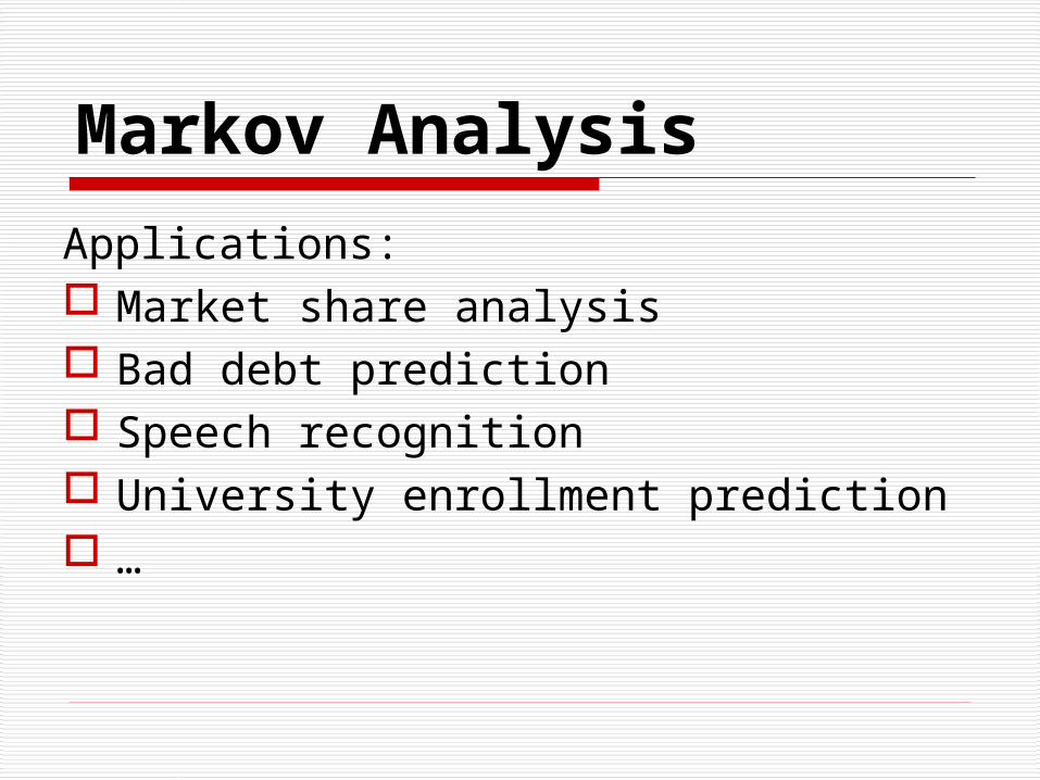
Markov Analysis

Applications: Market share analysis Bad debt prediction Speech recognition University enrollment prediction …

Markov Analysis Two competing manufacturers might

have 40% & 60% market share today. May be in two months time, their market shares would become 45% & 55% respectively

Predicting these future states involve knowing the system’s probabilities of changing from one state to another

Matrix of transition probabilities This is Markov Process

Markov Analysis1. A finite number of possible states.

2. Probability of change remains the same over

time.

3. Future state predictable from current state.

4. Size of system remains the same.

5. States collectively exhaustive.

6. States mutually exclusive.

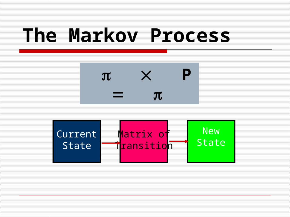
The Markov Process

Matrix ofTransition

NewState

CurrentState

P

Markov ProcessEquations

P11 P12 P13...P1n

P21 P22 P23...P2n

Pm1 ... Pmn

Matrix oftransition probabilities

= P =

(i) = State probabilities = [1 2 3 … n]

(i+1) = (i)P

Predicting Future States

Market Share of Grocery Stores

AMERICAN FOOD STORE: 40%

FOOD MART: 30%

ATLAS FOODS: 30%

∏(1)=[0.4,0.3,0.3]


28.031.041.0)2(

.6*.3.2*.3.1*.4

.2*.3*.7*.3.1*.4

.2*.3*.1*.3.8*.4)2(

6.2.2.

2.7.1.

1.1.8.

.3.3.4 )2(

)1()2(

6.2.2.

2.7.1.

1.1.8.

.3.3.4 (1)

iesprobabilit Stateπ

P

P


•Will this trend continue in the future?

•Is it an equilibrium state?

•WILL Atlas food lose all of its market share?

Markov Analysis: Machine Operations

P= 0.8 0.2

0.1 0.9State1: machine functioning correctly

State2: machine functioning incorrectly

P11 = 0.8 = probability that the machine will be correctly functioning given it was correctly functioning last month

∏[2]=∏[1]P=[1,0]P=[0.8,0.2]

∏[3]=∏[2]P=[0.8,0.2]P=[0.66,0.34]

Machine Example: Periods to Reach Equilibrium

Period

123456789

101112131415

State 1

1.0 .8

.66 .562

.4934 .44538

.411766 .388236 .371765 .360235 .352165 .346515 .342560 .339792 .337854

0.0 .2

.34 .438

.5066 .55462

.588234 .611763 .628234 .639754 .647834 .653484 .657439 .660207 .662145

State 2

Equilibrium Equations

1

and 1

:

:or

:Then

P , (i) :Assume

)()1(

22

1212

11

2121

2221212 ,2121111

22212121211121

2221

121121

p

p

p

p

Therefore

PPPP

PPPP

pp

pp

Pii

Markov System

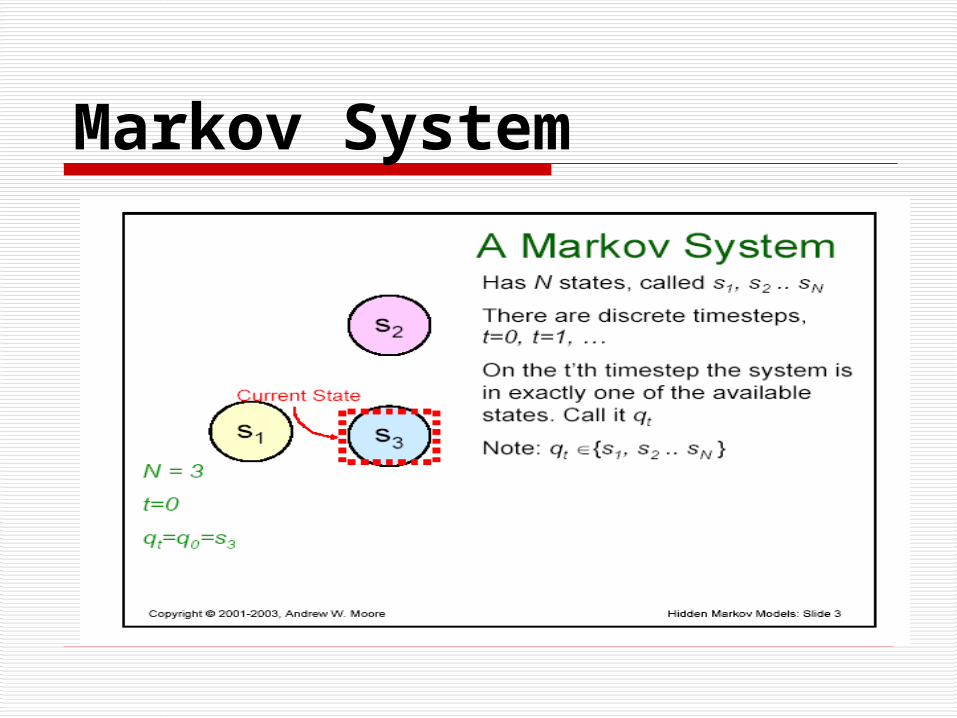
Markov System• At regularly spaced discrete times, the system undergoes a change of state (possibly back to same state)

• Discrete first order Markov Chain

P[qt=Sj|qt-1=Si,qt-2=Sk,…..]= P[qt=Sj|qt-1=Si]

• Consider only those processes in which the RHS is independent of time

• State transition probabilities are given by

aij = P[qt=Sj|qt-1=Si] 1<=i,j<=N

Markov Models A model of sequences of events where the probability

of an event occurring depends upon the fact that a preceding event occurred. Observable states: 1, 2, …, N Observed sequences: O1, O2, …, Ol, …, OT

P(Ol=j|O1=a,…,Ol-1=b,Ol+1=c,…)=P(Ol=j|O1=a,…,Ol-1=b)

Order n model A Markov process is a process which moves from

state to state depending (only) on the previous n states.

Markov Models

First Order Model (n=1) P(Ol=j|Ol-1=a,Ol-2=b,…)=P(Ol=j|Ol-1=a) The state of model depends only on its

previous state. Components: States, initial probabilities &

state transition probabilities

Markov Models Consider a simple 3-state Markov model of weather Assume that once a day (eg at noon), the weather is

observed as one of the folowiing: State 1 Rain or (snow) State 2 Cloudy State 3 Sunny

Transition Probabilities:0.4 0.3 0.30.2 0.6 0.20.1 0.1 0.8

Given that on day 1 the weather is sunny What is the probability that the weather for the next 7

days will be S S R R S C S?

Hidden Markov Model HMMs allow you to estimate

probabilities of unobserved events E.g., in speech recognition, the

observed data is the acoustic signal and the words are the hidden parameters

HMMs and their Usage HMMs are very common in

Computational Linguistics: Speech recognition (observed: acoustic

signal, hidden: words) Handwriting recognition (observed:

image, hidden: words) Machine translation (observed: foreign

words, hidden: words in target language)

Markov Model is used to predict what will come next based on previous observations.

However, sometimes, what we want to predict is not what we observed.

Example Someone trying to deduce the weather from a piece

of seaweed For some reason, he can not access weather

information (sun, cloud, rain) directly But he can know the dampness of a piece of

seaweed (soggy, damp, dryish, dry) And the state of the seaweed is probabilistically

related to the state of the weather

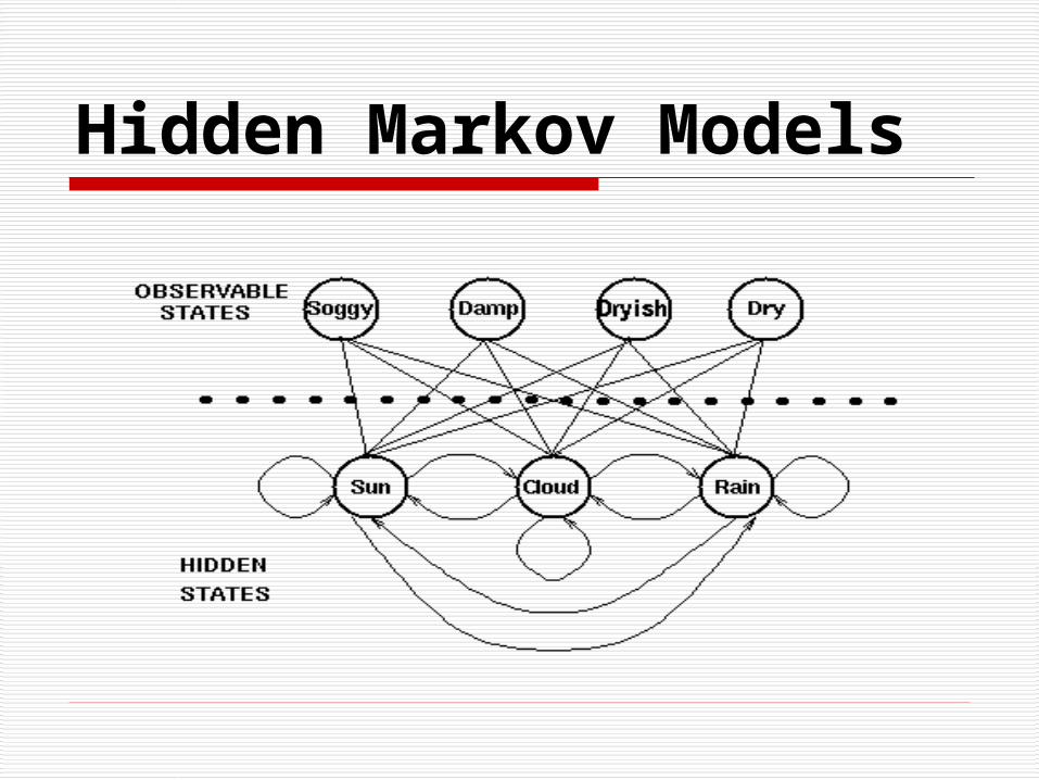
Hidden Markov Models


Hidden Markov Models are used to solve this kind of problems.

Hidden Markov Model is an extension of First Order Markov Model The “true” states are not observable directly

(Hidden) Observable states are probabilistic functions

of the hidden states The hidden system is First Order Markov


A Hidden Markov Model is consist of two sets of states and three sets of probabilities: hidden states : the (TRUE) states of a system that may

be described by a Markov process (e.g. weather states in our example).

observable states : the states of the process that are `visible‘ (e.g. dampness of the seaweed).

Initial probabilities for hidden states Transition probabilities for hidden states Confusion probabilities from hidden states to

observable states


Initial matrix

Transition matrix

Confusion matrix

The Trellis

Coin Toss Problem Observed Sequence: HHTTTHTTH….H How do we build an HMM to explain (model) the observed sequence?

What the states in the model correspond to? How many states should be there in the model?

Single biased coin is tossed 2 state model Each state corresponds to a side of the coin ( H or T) Resultant Markov model is observable Only unknown in the value of the bias

2 biased coins are tossed 2 states in the model Each state corresponds to a different, biased coin being tossed Each state characterized by prob. dist. Of Hs & Ts

3 biased coins are tossed

Coin Toss Problem Single biased coin is tossed

2 state model Each state corresponds to a side of the coin ( H or T) Resultant Markov model is observable Only unknown in the value of the bias

Coin Toss Problem 2 biased coins are tossed

2 states in the model Each state corresponds to a different, biased coin being tossed Each state characterized by prob. dist. Of Hs & Ts

Coin Toss Problem 3 biased coins are tossed

Coin Toss Problem Which model best matches the actual observation? 1coin model has only one unknown parameter – the bias 2 coin model has 4 unknown parameters 3 coin model has 9 unknown parameters Degrees of freedom Larger HMMs more capable of modeling a series of coin tossing

experiments?? Theoretically correct, but not practically Practical considerations impose limitations on the size of the HMM It might be the case that only 1 coin is being tossed

Urn & Coloured Balls Model

Urn & Coloured Balls Model State corresponds to a specific URN, and for which a

(ball) color probability is defined for each state Choice of URNS is dictated by the state transition

matrix of the HMM

Elements of an HMM N, number of states in the model, which are hidden Physical significance attached to the states Coin tossing experiment:

Each state corresponds to a distinct biased coin

Urn ball model State corresponds to urns

Generally the states are interconnected Ergodic Model

Elements of an HMM M, number of distinct observation symbols per state Coin tossing experiment:

Hs or Ts

Urn ball model Colors of the balls

Elements of an HMM A, state transition probability distribution

aij = P[qt+1=Sj|qt=Si] 1<=i,j<=N

Elements of an HMM Observation symbol probability distribution in state j

B={bj(k)}, where

Elements of an HMM The initial state distribution

HMM problems

HMMs are used to solve three kinds of problems Finding the probability of an observed sequence

given a HMM (evaluation); Finding the sequence of hidden states that most

probably generated an observed sequence (decoding).

The third problem is generating a HMM given a sequence of observations (learning). –learning the probabilities from training data.

HMM problems

HMM Problems1. Evaluation

Problem: We have a number of HMMs and a sequence

of observations. We may want to know which HMM most probably generated the given sequence.

Solution: Computing the probability of the observed

sequences for each HMM. Choose the one produced highest probability Can use Forward algorithm to reduce

complexity.

HMM problems2. Decoding

Problem: Given a particular HMM and an observation

sequence, we want to know the most likely sequence of underlying hidden states that might have generated the observation sequence.

Solution: Computing the probability of the observed

sequences for each possible sequence of underlying hidden states.

Choose the one produced highest probability Can use Viterbi algorithm to reduce the

complexity.

HMM Problems

the most probable sequence of hidden states is the sequence that maximizes :

Pr(dry,damp,soggy | sunny,sunny,sunny), Pr(dry,damp,soggy | sunny,sunny,cloudy), Pr(dry,damp,soggy | sunny,sunny,rainy), . . . . Pr(dry,damp,soggy | rainy,rainy,rainy)

HMM problems (cont.)

3. Learning Problem:

Estimate the probabilities of HMM from training data Solution:

Training with labeled data Transition probability P(a,b)=(number of transitions from

a to b)/ total number of transitions of a Confusion probability P(a, o)=(number of symbol o

occurrences in state a)/(number of all symbol occurrences in state a)

Training with unlabeled data Baum-Welch algorithm The basic idea

Random generate HMM at the beginning Estimate new probability from the previous HMM

until P(current HMM) – P( previous HMM) < e (a small number)

Designing HMM for an Isolated Word Recognizer

Vocabulary of V words Each word to be modeled by a distinct HMM For each word, we have a training data set of K

occurrences of each word (spoken by one or more talkers)

Each occurrence of the word constitutes an observation sequence

Observations are some appropriate representations of the characteristics of the word


To do isolated word speech recognition:

HMM Application:Parsing a reference string into fields

Problem Parsing a reference string into fields (author, journal, volume,

page, year, etc.)

Model as HMM Hidden states – fields (author, journal, volume, etc)

and some special characters ( “,”, “and”, etc.) Observable states – words Probability matrixes --learning from training data

Reference parsing Using Viterbi algorithm to find the most possible

sequence of hidden states for an observation sequence

Conclusions

HMM is used to model What we want to predict is not what we observed The underlying system can be model as first order Markov

HMM assumption The next state is independent of all states but its previous

state The probability matrixes learned from samples are the

actual probability matrixes. After learning, the probability matrixes will keep

unchanged

HIDDEN MARKOV MODELS Prof. Navneet Goyal Department of Computer Science BITS, Pilani Presentation...

Documents

Transcript of HIDDEN MARKOV MODELS Prof. Navneet Goyal Department of Computer Science BITS, Pilani Presentation...