Helsinki University of Technology

Department of Electrical and Telecommunications Engineering

Vesa Linja-aho

HOMOTOPY METHODS IN DC CIRCUIT ANALYSIS

Thesis submitted for examination for the degree of Master of Science inTechnology

Espoo 18.9.2006

Thesis supervisor:

Prof. Martti Valtonen

Thesis instructor:

Lic.Sc. (Tech.) Mikko Honkala

Helsinki University of Technology Abstract of

master’s thesis

Author: Vesa Linja-aho

Title: Homotopy Methods in DC Circuit Analysis

Date: 18.9.2006 Language: English Number of pages: 37

Department: Electrical and telecommunications engineering

Professorship: Circuit theory Code: S-55

Supervisor: Prof. Martti Valtonen

Instructor: Lic.Sc. (Tech.) Mikko Honkala

In this thesis, a comprehensive literature study and simulation-basedcomparison for using homotopy methods in DC circuit analysis was made.Homotopy methods are a subclass of continuation methods, which havebeen successfully used to solve nonlinear sets of equations.

Fixed-point, variable stimulus, and modified variable stimulus homotopyfunctions with plain Newton-Raphson, ordinary differential equation-based,and pseudo-arclength-based solver algorithms for finding DC operatingpoints for electric circuits were tested.

Plain Newton-Raphson and pseudo-arclength methods were implemented inMATLAB and tested with the MATLAB-APLAC interface. The simulationresults are discussed.

Keywords: Circuit simulation, homotopy methods, DC analysis

Teknillinen korkeakoulu Diplomityon

tiivistelma

Tekija: Vesa Linja-aho

Tyon nimi: Homotopiamenetelmat virtapiirien DC-analyysissa

Paivamaara: 18.9.2006 Kieli: Englanti Sivumaara: 37

Osasto: Sahko- ja tietoliikennetekniikka

Professuuri: Circuit theory Koodi: S-55

Valvoja: Prof. Martti Valtonen

Ohjaaja: TkL Mikko Honkala

Tassa diplomityossa suoritettiin kattava kirjallisuustutkimus ja simulaa-tiovertailu homotopiamenetelmista tasavirtapiirien analyysissa. Homo-topiamenetelmat ovat kontinuaatiomenetelmien alaluokka. Homotopi-amenetelmia on menestyksellisesti kaytetty epalineaaristen yhtaloryhmienratkaisemiseen.

Kiintopistehomotopiafunktio, muuttuvan heratteen homotopiafunk-tio ja modifioitu muuttuvan heratteen homotopiafunktio testattiinvirtapiiriyhtaloiden ratkaisemisessa. Ratkaisualgoritmeina kaytettiinNewton-Raphson-kontinuaatiota, pseudokaarenpituusalgoritmia ja differen-tiaaliyhtaloihin pohjautuvaa menetelmaa.

Newton-Raphson-kontinuaatio ja pseudokaarenpituusalgoritmi implemen-toitiin MATLABiin ja testattiin MATLAB-APLAC-rajapinnalla. Simuloin-tituloksia tarkasteltiin.

Avainsanat: Piirisimulointi, homotopiamenetelmat, DC-analyysi

Preface

”I devoted myself to study and toexplore by wisdom all that is done

under heaven. What a heavy burdenGod has laid on men!”

- The Holy Bible, NIV, Eccl. 1:13

I wish to thank professor Martti Valtonen and my instructor Mikko Honkalafor patiently supporting me with this endless-seeming project.

I deeply appreciate support from all my colleagues at the Circuit theory labora-tory, especially Luis Costa for helping me with the LATEX typesetting program.The great work atmosphere, especially the fun discussions at the coffee table,helped me withstand the moments when this project felt frustrating. Financialsupport received through MOSAICS project is acknowledged.

This work could not have been finished without support from my lovely wifeMinttu — thank you for your encouragement and help.

I dedicate this thesis to my dear parents Hannele, who died this year, andMartti, who died last year. You always supported me in my studies — so sadyou did not see me graduate.

And finally, to anyone who is starting his or her master’s thesis and reads this:choose to do your thesis as full-time employee, not part-time as I did. Theother work assignments will wait you, no matter how well-paid and interestingthey are.

Otaniemi, September 18, 2006

Vesa Linja-aho

iv

Contents

Abstract ii

Abstract (in Finnish) iii

Preface iv

Contents v

Symbols and notational conventions vii

1 Introduction 1

2 Background on DC Circuit Analysis 1

2.1 Circuit Simulation . . . . . . . . . . . . . . . . . . . . . . . . . 1

2.2 APLAC Circuit Simulation and Design Tool . . . . . . . . . . . 2

2.3 DC Analysis and Newton-Raphson Method . . . . . . . . . . . . 2

2.4 Convergence-Aiding Techniques . . . . . . . . . . . . . . . . . . 2

2.4.1 Model Damping . . . . . . . . . . . . . . . . . . . . . . . 3

2.4.2 Source Stepping . . . . . . . . . . . . . . . . . . . . . . . 3

2.4.3 Voltage Limiting . . . . . . . . . . . . . . . . . . . . . . 4

2.4.4 Diode Damping . . . . . . . . . . . . . . . . . . . . . . . 4

2.4.5 Norm Reduction . . . . . . . . . . . . . . . . . . . . . . 4

2.4.6 Temperature Sweeping . . . . . . . . . . . . . . . . . . . 5

3 Homotopy Methods 6

3.1 Bifurcation and Folds . . . . . . . . . . . . . . . . . . . . . . . . 7

3.2 Homotopy Function . . . . . . . . . . . . . . . . . . . . . . . . . 9

3.2.1 Fixed-Point Homotopy Function . . . . . . . . . . . . . . 9

3.2.2 Variable Stimulus Homotopy Function . . . . . . . . . . 10

3.2.3 Modified Variable Stimulus Homotopy Function . . . . . 11

3.2.4 Combinations and Other Homotopy Functions . . . . . . 11

3.3 Solving the Homotopy Equations . . . . . . . . . . . . . . . . . 12

v

3.3.1 Standard Newton–Raphson Solver . . . . . . . . . . . . . 12

3.3.2 ODE-based Solver . . . . . . . . . . . . . . . . . . . . . 13

3.3.3 Pseudo-arclength Solver . . . . . . . . . . . . . . . . . . 13

3.3.4 HOMPACK – A Suite of Solver Algorithms . . . . . . . 15

3.4 Practical Viewpoints . . . . . . . . . . . . . . . . . . . . . . . . 17

3.4.1 Selecting Parameters . . . . . . . . . . . . . . . . . . . . 17

3.4.2 Ensuring the Convergence . . . . . . . . . . . . . . . . . 17

4 MATLAB Tests 19

4.1 Experiment setup . . . . . . . . . . . . . . . . . . . . . . . . . . 19

4.1.1 MATLAB–APLAC Interface . . . . . . . . . . . . . . . . 19

4.1.2 Implementation and Benchmark Circuits . . . . . . . . . 19

4.2 A Simple Simulation Example . . . . . . . . . . . . . . . . . . . 20

4.3 Standard Newton-Raphson Solver . . . . . . . . . . . . . . . . . 22

4.3.1 The Fixed-Point Homotopy Function . . . . . . . . . . . 23

4.3.2 The Variable Stimulus Homotopy Function . . . . . . . . 24

4.3.3 The Modified Variable Stimulus Homotopy Function . . 25

4.3.4 Test for NR-Continuation with Equal Parameters . . . . 25

4.4 ODE-Based Curve Tracing . . . . . . . . . . . . . . . . . . . . . 25

4.4.1 The Fixed-Point Homotopy . . . . . . . . . . . . . . . . 25

4.5 Pseudo-Arclength Solver with the Planar Corrector . . . . . . . 27

4.6 Pseudo-Arclength Solver with the Spherical Algorithm . . . . . 27

5 Discussion 29

6 Conclusion 31

References 32

Appendix A 35

Appendix B 36

vi

Symbols and notational conventions

Symbolic Notations

x scalarx node voltage vectorddt

derivative with respect to t∂∂t

partial derivative with respect to tf(x) set of nodal equations for a circuitJ Jacobian matrixGmin the minimum conductance in model damping techniqueVT thermal voltage of a semiconductor diodeIS saturation current of a semiconductor diodeǫ current imbalance in norm reduction techniqueλ homotopy parameterH(x, λ) homotopy functiona initial guess vector for homotopy functionG conductance scaling diagonal matrix for homotopy functionu unit vector in λ − x hyperplane∆s step length in pseudo-arclength methods

Abbreviations

AC alternating currentAPLAC circuit simulator and design tool

(originally Analysis Program for Linear Active Circuits)BJT bipolar junction transistorDC direct currentJFET junction field effect transistorMATLAB Matrix Laboratory (a computer program)MOSFET metal-oxide semiconductor field effect transistorNR Newton–RhapsonODE ordinary differential equationSPICE Simulation Program with Integrated Circuit Emphasis

vii

1 Introduction

In computer-based circuit simulation, finding the DC operating point of thecircuit is usually the first step of all other analyses. Therefore, if the simulatorcannot find the operating point, also all other simulations are impossible torun.

Determining the DC operating point requires solving a set of nonlinear equa-tions. The most usual methods are based on Newton–Raphson iteration witha bunch of convergence-aiding techniques.

Strongly nonlinear circuits and circuits which have multiple DC operatingpoints are very difficult for conventional solver algorithms. One way to improveconvergence is to use so called homotopy methods. Homotopy methods can helpto find the DC operating point for a troublesome circuit.

For this thesis, homotopy methods have been studied and tested with trouble-some circuits. The practical testing of homotopy algorithms was carried outusing APLAC circuit simulation and design tool [1, 2] and MATLAB software.Before doing this, a comprehensive literature study on homotopy methods wascarried out.

The main goal of the research was testing the homotopy methods with practicalcircuits. The practical implementation of a homotopy method consists of twoparts: deciding which homotopy equation to use, and solving the equation.

2 Background on DC Circuit Analysis

2.1 Circuit Simulation

Circuit simulation is an important part of electronic circuit design at present.By simulating the operation of the circuit beforehand, the need for expensiveprototypes is avoided. Using circuit simulation, the design process is acceler-ated and designers can test circuits which can be practically impossible to testin real world [3]. For example, it can be simulated how a certain improvementin characteristics of semiconductor component will affect the performance of adevice. The simulation will help in deciding how much effort is reasonable totake in improving the certain characteristic.

Circuit simulation can be used to optimize the yield of the manufacturingprocess, thus reducing the manufacturing costs. Dealing with component valuetolerances is practically impossible without circuit simulation, especially whendesigning large circuits.

1

2.2 APLAC Circuit Simulation and Design Tool

APLAC is a flexible circuit simulator suite originally created by professorMartti Valtonen. Nowadays, the development is made under the AWR-APLACCorporation.

2.3 DC Analysis and Newton-Raphson Method

The problem of finding the DC operating point can be described as a set ofnonlinear equations

f (x) = 0 (1)

where x is a node voltage vector.

The basic method for numerically solving the circuit equations is the Newton–Raphson method [3, ch. 4.2]. The equation 1 is solved iteratively with theformula

x(j+1) = x(j) − [J(xj)]−1f (x(j)), (2)

where J represents the Jacobian matrix of the function f (x) and j is therunning index for the iteration count [6, ch. 5.4.3].

The Newton-Raphson method can be guaranteed to be globally convergent forsingle-BJT circuits [16]. In certain conditions described in [16], the convergencecan be guaranteed for most of the practical BJT-circuits.

The DC analysis in APLAC circuit simulator is carried out by solving modifiednodal equations of the circuit. The set of modified nodal equations is formedvia the gyrator transform. [2]

2.4 Convergence-Aiding Techniques

In DC analysis, Newton–Raphson algorithm converges well if the initial guessfor the operating point is good. For a computer program, it is very difficult tomake a good guess for the operating point. Additionally, almost all practicalcircuits are strongly nonlinear. An ordinary semiconductor diode, for example,has a very steep exponential characteristic function.

Because the convergence of the plain Newton–Raphson algorithm cannot beguaranteed for all practical circuits, a number of convergence-aiding methodshave been developed. Model damping, source stepping, voltage limiting, diodedamping, norm reduction, piecewise-linear analysis [4] and dogleg method [5]are in use in the APLAC circuit simulator.

2

No method guarantees convergence alone. APLAC uses different combina-tions of convergence-aiding techniques to find the operating point. Usuallythe source stepping method is the last resort when all the other methods fail[2].

Some of the convergence aiding techniques are introduced in the followingsections. They are described in [2]. One of the methods, the source steppingmethod, is a so called continuation method or homotopy method. Homotopymethods have been efficiently used to solve sets of nonlinear equations.

2.4.1 Model Damping

In model damping, every nonlinear static source in the circuit is shunted witha conductance having the value

G = 10mGmin, (3)

where Gmin is the minimum conductance in the circuit and m is an integer.Conductance G is also added between every node and ground.1 The defaultvalues for Gmin and m are 10−12 and 6, respectively. User can alter both of thevalues. The iteration of the DC operating point is started with the m given,and after the iteration converges, m is reduced by one. This is repeated, untilm = 0.

2.4.2 Source Stepping

In the source stepping method, all the voltage sources in the circuit are mul-tiplied by a constant k ∈ [0, 1]. When making a DC analysis, the iteration isstarted with k = 1 (the original circuit). If convergence is not achieved, theconstant k is decreased and a new iteration is attempted.

When the iteration converges, k is increased gradually, until k = 1. Theoperating point found with the previous convergent iteration is used as aninitial guess for the next iteration.

Source stepping method has an easy physical interpretation — the circuit is“powered up” gradually by increasing the source voltages. Source stepping isa very efficient method when dealing with strongly nonlinear circuits.

1A popular convergence aiding technique which consists only of adding small conduc-tances between all nodes and ground is called the Gmin stepping method [10].

3

2.4.3 Voltage Limiting

Voltage limiting is a simple method for preventing semiconductor componentsfrom switching on and off repeatedly during the iteration. The user can define aconstant Umax, which describes the maximum allowed voltage change betweeniteration cycles. If the voltage change between two iteration cycles exceedsUmax, all the voltages are multiplied with a constant β so that the maximumvoltage change is Umax:

un+1 = un + β(un+1 − un) (4)

where

β =Umax

max |un+1 − un|. (5)

If none of the voltage changes exceeds Umax, β = 1.

2.4.4 Diode Damping

Diode damping is a convergence improvement method for dealing with thesteep exponential characteristic curve of diodes. It is closely related to thevoltage limiting method. Every diode monitors its voltage, and the dampingfactor is calculated

β = 1, if un+1 ≤ VT ln

(

VT√2IS

)

(6)

and

β =VT ln(un+1−un

VT+ 1)

un+1 − un

, if un+1 > VT ln

(

VT√2IS

)

, (7)

where VT and IS are the thermal voltage and the saturation current of thediode, respectively. The new voltage is then calculated from the equation (4).

2.4.5 Norm Reduction

Norm reduction is practically equivalent to line search optimization. On eachiteration cycle, the current imbalance ε between the feeding and loading cir-cuits is monitored. If the current imbalance

ε = max

∣

∣

∣

∣

∣

I − i(u) − ∂i

∂u

∣

∣

∣

u=un

u

∣

∣

∣

∣

∣

(8)

increases, a damping factor β = 0.5 is applied. If the norm still increases,parabolic fitting is used in order to find a damping factor which reduces theerror.

The procedure is repeated until an error-reducing step length is found or themaximum error criteria is satisfied.

4

2.4.6 Temperature Sweeping

In the temperature-sweeping [8] method the temperature of the circuit is sweptfrom a certain value (usually zero) to the final value, which is the operatingtemperature of the circuit. The method requires that the component modelswork in the whole temperature range. For example, if a model is verified onlyto work at temperatures near room temperature, the temperature sweep hasno purpose. The temperature sweeping method is not implemented in APLACsimulator.

5

3 Homotopy Methods

“A continuous transformation from one function to another” is called a ho-motopy [7]. For this thesis, a number of scientific publications concerninghomotopy methods were examined.

Homotopy methods are a subset of continuation methods. In a continuationmethod, a solution of an algebraic nonlinear problem is treated as an instantof a dynamic problem [3]. For instance, the source stepping method is acontinuation method. Sweeping the source voltages from small values to thefinal value is like powering up the circuit.

In a homotopy method, an auxiliary equation is constructed for solving theoriginal problem. If the original problem is

f(x) = 0, (9)

one example of a homotopy equation for the problem is

H(x, λ) = λf(x) + (1 − λ)g(x) = 0. (10)

The idea of the homotopy method is the following: an easy function is chosen asg(x). After that, the parameter λ is swept from 0 to 1, so that the easy problemis continuously deformed into the original problem. The homotopy functionH(x, λ) may be constructed and solved in numerous ways. The concept ofusing a homotopy method for solving a set of nonlinear equations consists of

1. the formation of the homotopy function

2. choosing an efficient solver

3. making a working implementation of them.

If one of the three elements has problems, the whole homotopy method maynot work (Figure 1).

For normal circuit equations, the solutions for the homotopy function whenλ is swept form a continuous path in λ–x –plane. For example in [9], thehomotopy method is defined to be “the class of continuation methods wherethe homotopy parameter does not necessarily vary monotonically as the pathfrom the original solution to the final solution is followed”. According to thedefinition, the source stepping, for example, is not a homotopy method.

Homotopy methods can be divided into two groups. In natural parameterhomotopy methods, the homotopy parameter is a parameter with an obviousphysical interpretation. That is, for example, if we multiply the supply voltage

6

Figure 1: The ingredients of a well-working homotopy method.

of the circuit by λ [12]. The opposite of the natural parameter homotopy meth-ods are artificial parameter homotopy methods. The homotopy in Equation10 is a good example of an artificial parameter homotopy method.

Homotopy methods have been used successfully for improving convergence inDC circuit analysis [11, 14]. The main idea of homotopy methods is to convertthe set of circuit equations into a simple equation, and convert it graduallyinto the original equation set. The homotopy methods are less sensitive tothe initial guess than the bare Newton–Raphson method. Some homotopymethods can, with certain conditions, even be globally convergent [8].

The main drawback of homotopy methods is their computational intensity[11]. For example, curve–tracing methods which use predictor and correctorneed a lot of computing power. Other difficulties with practical use of homo-topy methods pertain to the implementation of homotopy methods [13]. Thealgorithm for solving the homotopy equations has to be carefully implemented.

Solving the DC operating point with a homotopy method is usually done bytracing the zero curve on the λ–x -plane. It is also possible to just step theembedded parameter forward. Numerical problems can be met if the zerocurve has sharp turns, or the homotopy curve bifurcates.

3.1 Bifurcation and Folds

The main purpose of homotopy methods is to find the DC operating point for acircuit, when all conventional methods fail. Homotopy methods can guaranteeconvergence, if implemented properly.

The two major problems homotopy solver algorithm may face are bifurcation

7

and folds in the homotopy curve. Bifurcation means that the homotopy curvein λ–x -plane splits into two or more curves, as in Figure 2.

0 0.2 0.4 0.6 0.8 1 1.20

0.1

0.2

0.3

0.4

0.5

0.6

0.7

0.8

0.9

1

λ

xBifurcation point

Figure 2: An example of bifurcation.

The bifurcation points can be troublesome for homotopy solvers. The solvercan diverge especially if the new branches of the curve diverge steeply fromeach other.

Folds in the homotopy curve may cause convergence problems too. If the curvefolds back steeply, as in Figure 3 while λ ≈ 10.5, the curve-tracing algorithmmay get stuck in the steep turn.

If a monotonic continuation, where λ always increases, is used, folds cause thealgorithm to fail. The reason for this is that if the λ always increases, thenumerical algorithm cannot follow the curve to the final solution. In Figure3, when λ is stepped third time, the algorithm seeks the solution near therightmost blue dot. Because λ cannot be decreased and the correct solutionfor that value of lambda is too far away, the algorithm will fail. The sourcestepping, for example, can suffer from this problem.

The problems caused by folds can be dealt with the so called curve tracingmethods. Instead of just stepping the parameter λ forward, the zero curve ofthe homotopy function is followed by a numerical algorithm. The simplest wayto do this is to take a step on the curve to the direction of the tangent vectorof the curve, and then use a corrector algorithm to get back on the originalcurve.

8

Very steep folds may cause problems even for curve tracing methods. One wayfor avoiding steep folds is to use complex parameter homotopies [21].

Figure 3: Monotonic continuation cannot handle folds.

3.2 Homotopy Function

In this thesis, the fixed-point, variable stimulus and modified variable stimulushomotopy functions described in e.g., [8] are reviewed and tested with differentsolvers.

3.2.1 Fixed-Point Homotopy Function

In a fixed-point homotopy, the original set of nodal functions

f (x) (11)

is transformed into homotopy function

H(x, λ) = (1 − λ)G(x − a) + λf(x), (12)

9

where x is the node voltage vector, λ ∈ [0, 1] is the homotopy parameter and a

is a randomly chosen vector. G ∈ Rn×Rn is an embedded conductance scalingparameter. When the homotopy parameter λ = 0, the function represents asimple circuit having node voltages described by a. When λ = 1, the originalfunction is obtained. By varying the parameter λ from 0 to 1, the simplecircuit is gradually transformed into the original (difficult) circuit.

The fixed-point homotopy has a simple physical representation. All the nodesin the circuit are connected to ground via a branch, which consists of a con-ductance λ

1−λGk in series with a voltage source having voltage ak, where k is

the index of the node.

The fixed-point homotopy can be considered as an improved version of theGmin stepping method. The voltage sources in series with the conductancesguarantee that the homotopy does not bifurcate. In a circuit with two or moreoperating points, the vector a defines which of the operating points is found.Bifurcation is described more accurately in Section 3.1. Homotopy curve mayalso fold back, which results in finding multiple operating points, if solver canhandle a folding curve.

Because of the simple physical interpretation, the fixed-point homotopy isrelatively easy to implement into a circuit simulator. Tampering of the existingmodels is not required.

3.2.2 Variable Stimulus Homotopy Function

Variable stimulus homotopy function is

H(x, λ) = (1 − λ)G(x − a) + f(x, λ), (13)

where the function f (x) is modified so that the node voltages of nonlinearelements are multiplied by the factor λ. Thus, the solution of the function atthe starting point λ = 0 is the solution of a linear circuit. Then the circuit isgradually converted to a more and more nonlinear circuit.

One disadvantage of the variable stimulus homotopy is that the simulatorcore and/or component models have to be tampered in order to multiply thevoltages of nonlinear circuit elements.

According to [8], one advantage of variable stimulus homotopy is a remark-able improvement of numerical stability when dealing with p-n junctions oftransistors and diodes.

10

3.2.3 Modified Variable Stimulus Homotopy Function

The modified variable stimulus homotopy is closely related to the variablestimulus homotopy. The equation is slightly different

H(x, λ) = (1 − λ)G(x − a) + f(λx). (14)

The main advantage of the modified variable stimulus homotopy is its simplic-ity. The circuit element models need no modifications, because all of the nodevoltages are multiplied with the same factor λ.

The modified variable-stimulus homotopy has been tested earlier [9] withADVICE–HOMPACK -interface. ADVICE is a circuit simulator and HOM-PACK is a suite of homotopy methods on Fortran language. The results werepromising. Two circuits which did not converge with the ordinary simulator,converged successfully with HOMPACK homotopy solver. For more detaileddescription of HOMPACK, see Chapter 3.3.4.

3.2.4 Combinations and Other Homotopy Functions

The homotopy function can be constructed in practically infinite number ofways. However, certain simplicity should be preserved. In addition to thethree homotopies presented, there are several others to mention.

In the variable gain homotopy the transistor forward current gains are multi-plied with the homotopy parameter

H(x, λ) = (1 − λ)G(x − a) + f (x, λα), (15)

where the α is a column vector consisting of the forward current gains ofthe transistors. According to [8], the variable gain homotopy is the fastestconverging homotopy for bipolar circuits. The implementation of the variablegain homotopy requires tampering the bipolar transistor models, which makesit harder to test.

In the hybrid homotopy introduced in [8], the starting point for variable gainhomotopy is calculated with the variable stimulus homotopy. In the same pa-per, an update homotopy, which is useful in determining how the DC operatingpoint varies over a range of circuit parameters (such as temperature or somecomponent values)

H(x, λ) = S(λ)G(x − a) + λf b(x) + (1 − λ)fa(x) (16)

is introduced. The function S(λ) is an any smooth function with S(0) =S(1) = 0, f a(x) is the nodal function for circuit just being calculated (for

11

example at temperature of 10 ◦C), and f b(x) describes the circuit that shouldbe solved with a new parameter value (for example at temperature of 15 ◦C).

In [14], a two-parameter homotopy algorithm called BLHOM for large-scaleMOSFET circuits, is presented. The method utilizes two parameters, λ1 andλ2, which control the drain–source characteristics and transfer characteristics,respectively. According to the publication, the homotopy converges on vir-tually all practical circuits and has led to significant savings in the AT&Tcompany.

Two interesting categories of homotopy methods to mention are complex pa-rameter homotopy methods and piecewise-linear homotopy methods. Accord-ing to [21], complex parameter homotopy methods are very effective whendealing with folds in the homotopy curve. Piecewise-linear homotopy methods[23] are considered less efficient than conventional predictor-corrector methods,but require no smoothness of the equations to be solved. Homotopy methodshave also been successfully used in fault diagnosis of piecewise-linear circuits[20].

3.3 Solving the Homotopy Equations

A robust solver is a necessity in order to utilize homotopy methods in con-vergence aiding. For this thesis, three different solvers were tested: a simpleNewton-Raphson continuation, an ordinary differential equation (ODE) -basedsolver, and pseudo-arclength continuation (with both spherical and planar cor-rector).

3.3.1 Standard Newton–Raphson Solver

The simplest way to utilize the homotopy equations is just stepping the homo-topy parameter, λ, forward and using the standard Newton-Raphson iteration.Starting from λ = 0, the homotopy parameter is increased a bit and the equa-tion is solved with Newton-Raphson iteration. This procedure is repeated untilλ = 1 and therefore the original problem solved. The result of previous itera-tion is used as an initial guess for next iteration cycle. The algorithm goes asfollows:

1. Start with λ = 0 and solve H(x, λ) = 0

2. Step λ forward.

3. Solve H(x, λ) = 0 with Newton–Raphson algorithm

4. If λ < 1, go to step 2.

5. Return the final solution

12

3.3.2 ODE-based Solver

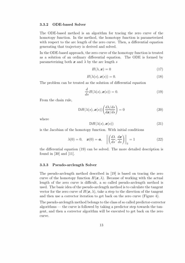
The ODE-based method is an algorithm for tracing the zero curve of thehomotopy function. In the method, the homotopy function is parameterizedwith respect to the arc length of the zero curve. Then, a differential equationgenerating that trajectory is derived and solved.

In the ODE-based approach, the zero curve of the homotopy function is treatedas a solution of an ordinary differential equation. The ODE is formed byparameterizing both x and λ by the arc length s

H(λ, x) = 0 (17)

H(λ(s), x(s)) = 0. (18)

The problem can be treated as the solution of differential equation

d

dsH(λ(s), x(s)) = 0. (19)

From the chain rule,

DH(λ(s), x(s))

(

dλ/ds

dx/ds

)

= 0 (20)

whereDH(λ(s), x(s)) (21)

is the Jacobian of the homotopy function. With initial conditions

λ(0) = 0, x(0) = a,

∣

∣

∣

∣

∣

∣

∣

∣

∣

∣

(

dλ

ds,dx

ds

)∣

∣

∣

∣

∣

∣

∣

∣

∣

∣

2

= 1 (22)

the differential equation (19) can be solved. The more detailed description isfound in [30] and [11].

3.3.3 Pseudo-arclength Solver

The pseudo-arclength method described in [19] is based on tracing the zerocurve of the homotopy function H(x, λ). Because of working with the actuallength of the zero curve is difficult, a so called pseudo-arclength method isused. The basic idea of the pseudo-arclength method is to calculate the tangentvector for the zero curve of H(x, λ), take a step to the direction of the tangentand then use a corrector iteration to get back on the zero curve (Figure 4).

The pseudo-arclength method belongs to the class of so called predictor-correctoralgorithms — the curve is followed by taking a predictor step towards the tan-gent, and then a corrector algorithm will be executed to get back on the zerocurve.

13

Figure 4: A predictor-corrector method.

Consider the zero curve of H(x, λ) in the λ−x hyperplane. Let the unit vectorbe

u = (ux, uλ). (23)

The tangent vector can be computed by solving a system of equations

dH(x,λ)dx

ux + dH(x,λ)dλ

uλ = 0

‖ux‖2 + u2λ = 1

. (24)

The solution of equation 24 is

uλ = ± 1√1+‖v‖2

2

ux = uλv

, (25)

where

v =−dH(x,λ)

dλdH(x,λ)

dx

. (26)

When the unit vectors ux and uλ have been calculated, the predictor step istaken

{

xi+1 = xi + ux∆sλi+1 = λi + uλ∆s

, (27)

14

where ∆s is the chosen step length. Because equation (25) has two possiblesolutions (the curve has two tangent vectors pointing in opposite directions),a test must be made in order to prevent the algorithm reverse the direction onthe curve. A simple way to do this is to evaluate, which of the selections takesus further from the previous point on the curve (if the wrong sign is selected,the new predicted point is very close to the previous predicted point). Then,a corrector algorithm (Newton-Raphson) is executed in order to get back onthe zero curve.

In order to get back on the solution curve, the corrector algorithm needs oneextra equation added to the system of original equations. The original systemconsists of n modified nodal equations and n unknown voltages, and we haveadded the homotopy parameter λ. To invoke the corrector algorithm, oneextra equation g(x, λ) is added. The most common choice is to use equation

g(x, λ) = u · ((xi+1, λi+1) − (xi, λi)) − ∆s = 0 (28)

which means that the next point lies on a hyperplane perpendicular to theunit tangent vector u.

Using a hyperplane as the additional equation may cause problems if the zerocurve of H(x, λ) has very steep turns on it. For example, if the curve makes asmall-radius 180 degrees turn, the hyperplane doesn’t intersect the zero curveat all and the corrector will fail. Other choice is to use a hyperball instead ofa hyperplane [22]. A ball will always intersect the zero curve at two points.The equation for the hyperball condition is

g(x, λ) = (x1 − c1)2 + (x2 − c2)

2 + . . . + (xn − cn)2 + (λ− λn)2 − r2 = 0, (29)

where cn corresponds to the previous point on the zero curve. The hyperballwill always intersect the zero curve in two points, regardless of the shape ofthe curve (Figure 5).

After selecting the additional equation, the system of n+1 unknowns and n+1equations is to be solved, to get back to the zero curve. The most commonalgorithm is the Newton-Raphson, introduced in the Chapter 2.3:

[

dH(x,λ)dx

dH(x,λ)dλ

dg(x,λ)dx

dg(x,λ)dλ

] [

xj+1 − xj

λj+1 − λj

]

= −[

H(x, λ)g(x, λ)

]

. (30)

3.3.4 HOMPACK – A Suite of Solver Algorithms

HOMPACK [29] is a suite of program codes in FORTRAN language. InHOMPACK, three different methods for solving systems of nonlinear equations

15

Figure 5: The hyperball condition for corrector.

are implemented: ODE-based, normal flow and augmented Jacobian matrixmethod. [30]. The HOMPACK algorithms have been successfully used to findDC operating points in a circuit simulator [34].

HOMPACK is designed for artificial parameter homotopies and it cannot han-dle homotopy curves which have bifurcations.

The ODE-based solver utilizes the same technique introduced in Chapter 3.3.2– the zero curve of the homotopy function is treated as a solution of an ordinarydifferential equation.

The normal flow algorithm is based on a concept called the Davidenko flow:when parameter a of the homotopy function is varied, the zero curve of thehomotopy function H(x, λ) also varies. This family of zero curves is knownas Davidenko flow. In the normal flow algorithm, the corrector iterates backon the zero curve along flow, which is normal to the Davidenko flow. Theprinciple of normal flow method is illustrated in [31].

The augmented Jacobian algorithm uses a Hermite cubic predictor and a quasi-Newton corrector, and the tangent vector of the zero curve is augmented intothe Jacobian matrix of the homotopy map. The augmented Jacobian algorithmis a modified version of an algorithm known as PITCON [32].

16

3.4 Practical Viewpoints

3.4.1 Selecting Parameters

For the fixed-point homotopy, the variable stimulus homotopy and the modi-fied variable stimulus homotopy, the formation of homotopy function has twocircuit-specific parameters: the initial voltage vector a and the conductancescaling matrix G. Determining values for these parameters has a significanteffect in ensuring fast convergence.

The randomness of a also guarantees a bifurcation-free path. It will alsoprevent finding the non-stable operating point of the circuit.

One difficulty with handling the homotopy function is the choice of the impedancescaling matrix G. It may be hard to automatically calculate reasonable val-ues. In [9], the matrix G was chosen to be a diagonal matrix with constantentries. The value for elements should correlate with the average impedancelevel of the circuit. For example, in a circuit dealing with power electronicsand low impedances like less than ten ohms, adding conductances of 1 mS maynot linearize the circuit and aid convergence adequately. Because it is hard todefine good separate values for diagonal elements of G, choosing all of themto be the same is a rational choice. In the simulation examples, the value ofthe diagonal elements is denoted with G.

The choice of vector a has also an impact on convergence – it defines thestarting point of the homotopy path. For fixed–point, variable stimulus, andmodified variable stimulus homotopies, the solution for H(x, λ) = 0 for λ = 0is x = a. Selection of the parameter defines also, which operating point isfound, if the circuit has multiple operating points. If a curve tracing methodwhich can find multiple operating points is used, the vector a will determinethe starting point for the homotopy curve and affect the shape of the homotopycurve. Therefore, a determines, which of the operating points are found. Forexample, if the circuit has 11 operating points, three of them can be foundwith a certain value of a and two of them with a different value of a. How thevalue of a affects, depends on the circuit topology.

3.4.2 Ensuring the Convergence

The main advantage of homotopy methods is their robustness. The fixed-point, variable stimulus, and modified variable stimulus homotopies can beguaranteed to be globally convergent with certain conditions described in [15].

The homotopy method has to be implemented carefully in order to ensure con-vergence. In [15] it has been proven that the three homotopy functions studiedin this thesis are globally convergent for a circuit satisfying passivity and no-gain properties. Almost all practical circuits fulfill these requirements. All

17

circuits consisting of non-negative resistors, diodes, tunnel diodes, thyristors,BJTs, MOSFETs and JFETs are passive and possess the no-gain property[15].

18

4 MATLAB Tests

Some of the homotopy methods reviewed were tested on actual circuits withthe MATLAB–APLAC interface. The fixed-point homotopy function, vari-able stimulus homotopy function, and modified variable stimulus function weretested with a Newton–Raphson solver. Additionally, the fixed-point homotopyfunction was tested with a pseudo-arclength (both with planar and sphericalcorrector) and the ODE-based algorithm.

4.1 Experiment setup

4.1.1 MATLAB–APLAC Interface

The tests for the homotopy methods were run on a specific MATLAB–APLAC–interface developed in the Circuit theory laboratory of the Helsinki Universityof Technology . The interface allows for using the MATLAB language to testnumerical methods with circuits described in the APLAC input language.

The interface takes node voltages as an input, and returns the values of thecircuit equations as well as the Jacobian matrix. Programming and testingnumerical methods with MATLAB is more convenient in comparison with C-language programming, although the interface sets certain limitations for themaximum size of the benchmark circuit. The interface also slows down thecomputing.

The availability of source code of the simulator is an essential thing in testingof the homotopy methods. For example it is also possible to import circuit de-scription files of the popular SPICE circuit simulator, which makes it possibleto run tests with different kind of circuits. Benchmarking circuit descriptionfiles for SPICE are widely available.

4.1.2 Implementation and Benchmark Circuits

The algorithms for testing a simple Newton-Raphson and pseudo-arclengthmethod were implemented. The source codes are presented in appendices Aand B, respectively. Tests for ODE-based method were made with a readyMATLAB source code by professor Heath Hoffmann [33]. The source codewas modified to use sparse matrices. The solver utilizes a variable step 4thorder predictor-corrector method to trace the solution curve.

Combinations of homotopy functions and solvers were tested with 12 circuits.The circuits used for testing and benchmarking the methods are summarizedin Table 1. The circuit schmitt.i is a simple circuit described in [15] and thecircuit ref6.i is a circuit with 11 DC operating points, described in [17].

19

Table 1: Summary of benchmark circuits

Name Nodes Diode BJT MOS OpAmppalikka.i 2 1 - - -simdc.i 3 - 1 - -toronto.i 26 - - 58 -voter.i 1710 - - 1710 -flipflop.i 5 - 2 - -globtest.i 113 - 17 42 -dcprob.i 475 - 104 41 4ssjudc.i 653 - 55 151 - -schmitt.i 6 - 2 - -ref6.i 17 3 6 - -dc demo.i 129 3 17 - -dcprob2.i 487 - 104 41 4

The following simulation sets were made:

• A simple simulation example to demonstrate the effect of initial guess.

• A test set for simple NR continuation to qualitatively test their capabil-ities

• A test set for simple NR continuation with fixed set of parameters

• A test set with Hoffmann’s ODE solver

• A test set with pseudo arclength solver, with planar and spherical cor-rectors

4.2 A Simple Simulation Example

In order to better understand the homotopy methods, a test for a simplenonlinear set of equations was carried out with MATLAB. Consider the set ofequations

{

x2 + y2 − 1 = 0−x2 + y = 0

, (31)

which describes a unity circle and parabola crossing each other in two points

y =

√5 − 1

2≈ 0.61803, x = ±

√√5 − 1

2≈ ±0.78615 (32)

20

0 1 2 3 4 5 6 7 8 9 10 11−2

−1.5

−1

−0.5

0

0.5

1

1.5

2

λ

x,y

xy

Figure 6: Fixed-point homotopy curves of Equation 31.

0.92 0.94 0.96 0.98 1 1.02 1.04 1.06 1.08

−1

−0.5

0

0.5

1

λ

x,y

xy

y=0.6180

x=0.7862

x=−0.7862

Figure 7: The solution is found at λ = 1.

21

0 0.1 0.2 0.3 0.4−30

−20

−10

0

10

20

30

λ

x,y

xy

Figure 8: Diverging homotopy.

The ODE-based solver by Heath Hoffmann [33] was used in tracking the zerocurve. The fixed-point homotopy was used, resulting in function

{

(1 − λ)(x − a1) + λ(x2 + y2 − 1 ) = 0(1 − λ)(x − a2) + λ(−x2 + y ) = 0

. (33)

The initial guess is important for finding the solutions. For example,ifthe initial guess is [a1 = 0.1, a2 = −0.1], the algorithm will find both thesolutions. If the initial guess is [a1 = 3, a2 = 4], the homotopy curve will foldback before λ = 1 and none of the solutions is found (see Figure 8). Resultsfor different values of a are collected in Table 2.

4.3 Standard Newton-Raphson Solver

The standard Newton-Raphson combined with homotopy functions is not anefficient way to solve the circuit equations. The main drawback of the algo-rithm is that it is not able to deal with foldbacks of the curve.

Three homotopy equations were tested: the fixed-point homotopy, the variablestimulus homotopy, and the modified variable stimulus homotopy.

Newton-Raphson continuation was tested using following values: the step forλ = 0.05, the conductance G = 10−2 and the criterion for terminating thecorrector iteration is that the norm of the function is smaller than 10−5. Thenumber of iterations depends on initial guess a. The solver was run five timesand the average is written on Table 3. The range for initial guess was a ∈ [0, 1].

22

Table 2: The effect of initial guess

a1 a2 Solutions found0.1 0.0 Positive0.0 0.1 Positive0.1 0.1 Positive0.0 -0.1 Both-0.1 0.0 Positive-0.1 -0.1 Both0.1 -0.1 Both-0.1 0.1 Both1.2 1 Both1 1.2 Both3 4 None

Table 3: The standard Newton-Raphson continuation - the number of Jacobianevaluations.

Fixed-point Variable stimulus Mod. variable stimuluspalikka.i 50 154 369simdc.i 82 58 289toronto.i 63(1 57 367voter.i fail fail failflipflop.i 70 72 331globtest.i fail fail faildcprob.i fail fail failssjudc.i fail fail failschmitt.i 72 90 1071ref6.i 143(1 452(1 994dc demo.i fail fail faildcprob2.i fail fail fail

1 Converged only after modifications to certain parameters.

4.3.1 The Fixed-Point Homotopy Function

Toronto.i required setting G = 10−4 in order to converge. Voter.i caused afloating point error near λ = 1. Both of the stable operating points of flipflop.iare found. The operating point which is found depends on the initial guess ofa.

Globtest.i has a nearly singular Jacobian at λ = 0.95. Dcprob.i will fail at

23

λ = 0.65 for the same reason. Ssjudc.i is even more difficult, it will fail in anearly singular Jacobian matrix when λ = 0.05.

MATLAB detects the (nearly) singularity of Jacobian matrix from the con-dition number of the matrix. For a well-conditioned matrix, the conditionnumber is close to 1. For a nearly singular matrix, the condition numberis very large, 10100 for example. The most common reason for the singularJacobian is that the iteration diverges.

The schmitt.i circuit has two operating points, of which just one is found withthe parameters described. However, if the range of the initial guess is extendedto a ∈ [0, 2], the other operating point is found, too.

The circuit ref6.i has numerical problems at λ = 1. The Jacobian remainsnon-singular but the iteration does not converge. The problem can be workedaround by raising the norm condition (the criteria for stopping the iterationbased on the norm of the homotopy function) from 10−5 → 10−4 and changingthe range of initial guess to a ∈ [0, 10]. In this manner, at least four differentoperating points (of 11 possible) are found.

The dc demo.i first converges well but at λ = 1 a floating point error occurs dueto nearly singular Jacobian matrix. The circuit dcprob2.i has similar problemsat λ = 0.9.

4.3.2 The Variable Stimulus Homotopy Function

Palikka.i and simdc.i converged without problems. Toronto.i converged with-out the modifications needed in fixed-point homotopy. Some of the initialguesses resulted in numerical failure due to nearly singular Jacobian matrix.

Voter.i has a nearly singular Jacobian near λ = 1, and fails to converge. Forflipflop.i, both of the stable operating points are found.

Simulation of circuits globtest.i, dcprob.i and ssjudc.i fail in similar manner asin fixed-point homotopy. Both of the operating points of the Schmitt triggerare found when the initial voltage vector range is extended to a ∈ [0, 2].

The circuit ref6.i needs the initial voltage vector values to be a ∈ [0, 10] inorder to converge. Unlike in fixed-point homotopy, the iteration stop criterianeeds no changes. Unfortunately, only one operating point is found. Someiterations do not converge. If the stopping criteria for function norm is alteredto 10−4, three more operating points are found.

The circuits dc demo.i and dcprob2.i fail. The iteration does not converge atλ = 1.

The variable stimulus homotopy doesn’t seem to have any remarkable advan-tages when compared to the fixed-point homotopy.

24

4.3.3 The Modified Variable Stimulus Homotopy Function

The modified variable stimulus homotopy seems to converge very poorly, if Gis few decades smaller than 1. For example, palikka.i did not converge after10000 iterations. Therefore, value 1 was used.

The simple circuits palikka.i and simdc.i did converge well. The voter.i didconverge extremely slowly and resulted in a numerical failure due to closelysingular Jacobian matrix. Both of the operating points of flipflop.i are found.

Globtest.i will fail at λ = 0.95 and the circuits dcprob.i and ssjudc.i fail too,all due to closely singular Jacobian matrix. For schmitt.i the initial voltagerange must be a ∈ [0, 4] in order to find both of the operating points.

The circuit ref6.i converges, but only one operating point is found. Dc demo.iand dcprob2.i both fail due to nearly singular Jacobian.

Combination of the Newton-Raphson solver and the modified variable stimulushomotopy seem to be inefficient if compared to the other two methods, becausemore iterations are needed, see Table 3.

4.3.4 Test for NR-Continuation with Equal Parameters

Some methods, which do not converge, can be made convergent by adjustingthe error criteria, step length, or the conductance scaling factor. However,to compare objectively the efficiency of the methods, a test with constantparameters is made. The results are shown in Table 4. The values are anaverage of five different solver runs. The source code for the method is includedin Appendix A.

4.4 ODE-Based Curve Tracing

The ODE-based homotopy solver was used with default tolerance options withthe fixed-point homotopy function and two different values for G. The sum-mary of Jacobian evaluations needed for finding the DC operating point (orthe first DC operating point, if multiple operating points exist) is presented inTable 5. The values are calculated as an average of five different solver runs.

4.4.1 The Fixed-Point Homotopy

The operating points of palikka.i and simdc.i are found easily. The operatingpoint of toronto.i is found easily, but the solver experiences numerical oscil-lation at λ = 1. That is, the zero curve is traced many times over the lineλ = 1, so that the solver finds the same operating point about ten times. The

25

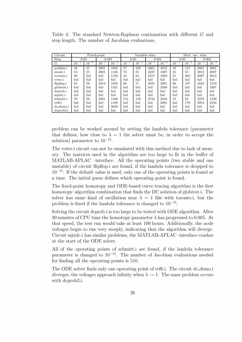
Table 4: The standard Newton-Raphson continuation with different G andstep length. The number of Jacobian evaluations.

Circuit Fixed-point Variable stim. Mod. var. stimStep 0.05 0.001 0.05 0.001 0.05 0.001G 10−1 10−3 10−1 10−3 10−1 10−3 10−1 10−3 10−1 10−3 10−1 10−3

palikka.i 46 47 2001 1092 57 339 2001 4072 49 147 2001 2001simdc.i 53 55 2001 1126 73 55 2227 1007 55 55 2012 2007toronto.i 46 fail fail 1103 44 64 2217 1003 51 263 2007 2012voter.i fail fail fail fail fail fail fail fail fail fail fail failflipflop.i 62 59 2013 1059 69 71 2021 2001 60 107 2022 1319globtest.i fail fail fail 1321 fail fail fail 2568 fail fail fail 3287dcprob.i fail fail fail fail fail fail fail fail fail fail fail failssjudc.i fail fail fail fail fail fail fail fail fail fail fail failschmitt.i 70 56 2001 1106 151 159 2734 2524 55 82 2270 1430ref6.i fail fail fail 1198 fail fail fail 2001 fail 178 3954 2192dc demo.i fail fail fail 2649 fail fail fail fail fail fail fail faildcprob2.i fail fail fail fail fail fail fail fail fail fail fail fail

problem can be worked around by setting the lambda tolerance (parameterthat defines, how close to λ = 1 the solver must be, in order to accept thesolution) parameter to 10−15.

The voter.i circuit can not be simulated with this method due to lack of mem-ory. The matrices used in the algorithm are too large to fit in the buffer ofMATLAB-APLAC –interface. All the operating points (two stable and oneunstable) of circuit flipflop.i are found, if the lambda tolerance is dropped to10−15. If the default value is used, only one of the operating points is found ata time. The initial guess defines which operating point is found.

The fixed-point homotopy and ODE-based curve tracing algorithm is the firsthomotopy–algorithm combination that finds the DC solution of globtest.i. Thesolver has same kind of oscillation near λ = 1 like with toronto.i, but theproblem is fixed if the lambda tolerance is changed to 10−15.

Solving the circuit dcprob.i is too large to be tested with ODE algorithm. After30 minutes of CPU time the homotopy parameter λ has progressed to 0.005. Atthat speed, the test run would take at least 100 hours. Additionally, the nodevoltages begin to rise very steeply, indicating that the algorithm will diverge.Circuit ssjudc.i has similar problems, the MATLAB-APLAC -interface crashesat the start of the ODE solver.

All of the operating points of schmitt.i are found, if the lambda toleranceparameter is changed to 10−15. The number of Jacobian evaluations neededfor finding all the operating points is 510.

The ODE solver finds only one operating point of ref6.i. The circuit dc demo.idiverges, the voltages approach infinity when λ → 1. The same problem occurswith dcprob2.i.

26

Table 5: The ODE-based homotopy method with different values of G.

G = 0.1 G = 0.001palikka.i 83 115simdc.i 207 260toronto.i 477 470voter.i fail (memory)flipflop.i 197 184globtest.i 1372 1334dcprob.i fail (too slow to be tested)ssjudc.i fail (program crash)schmitt.i 158 175ref6.i 344 310dc demo.i fail faildcprob2.i fail fail

4.5 Pseudo-Arclength Solver with the Planar Corrector

The pseudo-arclength solver introduced in Chapter 3.3.3 was tested with dif-ferent step size and the conductance scaling factor G. The results are in Table6. The method seems to be computationally efficient, and choice of G has nosignificant influence in the count of Jacobian evaluations. The source code forthe solver is included in Appendix B.

4.6 Pseudo-Arclength Solver with the Spherical Algo-rithm

A spherical algorithm is a predictor-corrector method for curve tracing. Theoutlines of the algorithm are presented at the end of Chapter 3.3.3. The testswere run for two different values for G and sphere radius. The results arepresented in Table 7.

27

Table 6: The arclength algorithm for fixed-point homotopy function with dif-ferent G and step length.

Circuit G = 0.1 G = 0.001Step 0.2 0.05 0.2 0.05

palikka.i 78 306 84 314simdc.i 93 247 71 77toronto.i 96 552 151 626voter.i fail fail fail failflipflop.i 65 317 87 301globtest.i fail fail 307 faildcprob.i fail fail fail failssjudc.i fail fail fail failschmitt.i 106 583 153 581ref6.i 215 1011 239 1235dc demo.i fail fail fail faildcprob2.i fail fail fail fail

Table 7: The Spherical algorithm and fixed-point homotopy function withdifferent radius of sphere and different values of G.

Circuit G = 0.1 G = 0.01Radius 0.01 0.005 0.01 0.005

palikka.i 1383 2942 fail 4553simdc.i 1543 2397 fail failtoronto.i 2605 6082 fail failvoter.i fail fail fail failflipflop.i 1162 2294 fail failglobtest.i fail fail fail faildcprob.i fail fail fail failssjudc.i fail fail fail failschmitt.i 3297 6459 fail 7758ref6.i 4633 8223 fail faildc demo.i fail fail fail faildcprob2.i fail fail fail fail

28

5 Discussion

In the literature, the homotopy methods are mentioned to be globally conver-gent. In theory, that is the fact. In practice, while tracing the zero curve ofthe homotopy function, the usual numerical problems are encountered. TheJacobian may be nearly singular near λ = 1. The zero curve has very steepfolds which cause the method to jump back on a point on the curve alreadytraced and therefore the algorithm will end up in an endless loop.

As with the plain Newton–Raphson method without homotopy implementa-tion or any other convergence-aiding technique, the homotopy methods seemto be very sensitive to the initial guess a. A good starting point is essential forfast convergence of the algorithm [25, 27]. For example, the circuits schmitt.iand ref6.i failed to converge on some initial guesses.

The most common problem with the curve tracing methods tested, was singu-larity or nearly singularity (condition number > 1090) of the Jacobian matrixnear the final solution λ = 1. The actual reasons of singularity are hard to findout for a set of hundreds of very complex nonlinear equations. One possiblereason may be high-impedance nodes in the circuit [26].

One goal for this thesis was to try to find out which homotopy method (ormethods) would be good enough to implement into the APLAC circuit simu-lator. Based on this thesis, the pseudo-arclength looks to be the most robustmethod for such implementation.

An efficient algorithm for step length control is a necessity when implementinghomotopy methods into a production version of a circuit simulator. In thisthesis, the step length was kept constant, but in order to save computationtime and improve accuracy at problem points on the zero curve, an efficientimplementation of step control algorithm should be reviewed. A good startingpoint for such a study would be [24].

The main problems confronted with testing the homotopy methods were nu-merical problems while tracing the zero curve of the homotopy function.

In the MATLAB–APLAC -interface, all the other convergence-aiding tech-niques implemented in APLAC were not in use. By implementing a homotopymethod directly into the simulator core (written in C programming language),the convergence-aiding techniques already implemented would be used to im-prove the numerical stability of the homotopy algorithm.

In [21] it is stated that complex parameter homotopy methods can find allsolutions of circuit without passing through folds or singular points. Thecomplex parameter homotopy methods would be worth deeper study and im-plementation tests. Another interesting kind of homotopy method for auto-matically finding all the DC operating points for circuits is described in [28].

29

The disadvantage of the method is that implementation requires tamperingthe component models of the nonlinear elements in the circuits.

It may be also worth to test calling HOMPACK or PITCON source codesdirectly from the simulator.

30

6 Conclusion

In this thesis, improving the convergence of DC analysis of a circuit simulatorby using homotopy methods was studied.

A literature review about homotopy methods in finding DC operating points ofelectric circuits was made. Three methods of constructing homotopy functionsand three methods for solving them were reviewed more closely and tested withAPLAC circuit simulator utilizing the MATLAB–APLAC -interface developedin the Circuit Theory laboratory of the Helsinki University of Technology.

Two solver algorithms were implemented in MATLAB language and one readyalgorithm was tested. The results from the MATLAB tests were reviewed.

According to MATLAB tests, choosing the homotopy function is not a crucialpart of a successful homotopy method. The solver algorithm, which is capableof dealing with problematic points on the zero curve, is a necessity for anefficient homotopy method.

The succession of the homotopy methods tested depends on the initial guessa of the homotopy path, especially with large and complex circuits.

The fixed-point homotopy method was found to be robust, easy to implement,and computationally efficient. All the homotopy methods were clearly helpfulin improving convergence — the circuit simdc.i, for example, does not convergewith ordinary Newton–Raphson iteration.

The arclength continuation method with planar corrector turned out to beefficient and stable when tracing the zero curve of the fixed-point homotopyfunction.

The homotopy methods were tested without any other convergence-aidingmethods. Homotopy methods combined with other convergence-aiding tech-niques have potential to improve the DC analysis convergence drastically inAPLAC circuit simulator.

31

References

[1] Aplac Solutions Corporation, Finland, APLAC 8.00 Reference Manualand User’s manual, 2004, http://www.aplac.com.

[2] M. Valtonen, P. Heikkila, H. Jokinen, and T. Veijola, “APLAC – object-oriented circuit simulator and design tool,” in Low-power HF Microelec-tronics: a Unifed Approach (G. A. S. Machado, ed.), pp. 333-372, IEE,1996.

[3] J. Ogrodzki, Circuit Simulation Methods and Algorithms, CRC Press Inc.,1994.

[4] J. Roos, “Improving the Speed and Convergence of DC Analysis by Meansof Self-Generating Lookup Tables and Piecewise-Linear Analysis,” Doc-toral thesis, Helsinki University of Technology, Espoo, 1999.

[5] M. Honkala, J. Roos, and V. Karanko, “On Nonlinear Iteration Meth-ods for DC Analysis of Industrial Circuits”, in Mathematics in Industry8: Progress in Industrial Mathematics at ECMI 2004 (A. Di Bucchian-ico, R. M. M. Mattheij, and M. A. Peletier, ed.), pp. 144-148, Springer,Berlin/Heidelberg, 2006.

[6] L.O. Chua and P.-M. Lin, Computer-Aided Analysis of Electronic Circuits:Algorithms & Computational Techniques, Prentice & Hall Inc., 1975.

[7] E. W. Weisstein, CRC Concise Encyclopedia of Mathematics, CRC Press,1999.

[8] L. Trajkovic, R. C. Melville and S. C. Fang, “Finding dc operating pointsof transistor circuits using homotopy methods,” Proc. IEEE Int. Symp.Circuits and Systems, Singapore, June 1991, pp. 758-761.

[9] L. Trajkovic, R. C. Melville and S. C. Fang, “Improving dc convergencein a circuit simulator using a homotopy method,” Proc. IEEE CustomIntegrated Circuits Conference, San Diego, CA, May 1991, pp. 8.1.1-8.1.4.

[10] Cadence Design Systems, USA, PSpice Convergence Guide, 2003,http://www.orcad.com

[11] A. Dyess, E. Chan, H. Hofmann, W. Horia, and L. Trajkovic, “Simpleimplementations of homotopy algorithms for finding dc solutions of non-linear circuits,” Proc. IEEE Int. Symp. Circuits and Systems, Orlando,FL, June 1999, vol. VI, pp. 290–293.

32

[12] R. C. Melville, L. Trajkovic, S. C. Fang, and L. T. Watson, “Artificialparameter homotopy methods for the dc operating point problem,” IEEETrans. on CAD, vol. 12, pp. 861–877, June 1993.

[13] L. Watson, “Globally Convergent Homotopy Methods,” SIAG/OPTViews-and-News, vol. 11, pp. 1–6, April 2000.

[14] J. S. Roychowdhury, R. C. Melville, “Homotopy techniques for obtaining aDC solution of large-scale MOS circuits,” Proceedings of the 33rd AnnualConference on Design Automation, United States, pp. 286-291, June 1996.

[15] L. Trajkovic, R. C. Melville and S. C. Fang, “Passivity and no-gain prop-erties establish global convergence of a homotopy method for dc operatingpoints,” Proc. IEEE Int. Symp. Circuits and Systems, New Orleans, LA,May 1990, pp. 914-917.

[16] C. P. Reames and A.N. Willson, Jr., “Global Convergence of Newton’sMethod in the DC analysis of Single-Transistor Networks,” ElectronicsLetters, vol. 18, no. 12, pp. 519-520, June 1982.

[17] K. Yamamura, T. Sekiguchi and Y. Inoue, “A Fixed-Point HomotopyMethod for Solving Modified Nodal Equations,” IEEE Transactions onCircuits and Systems, vol. 46, no. 6, June 1999.

[18] M. M. Green, “An Efficient Continuation Method for Use in GloballyConvergent DC Circuit Simulation,” ISSSE ’05 Proceedings, pp. 497-500,October 1995.

[19] P. Rodrigues, Computer-aided analysis of nonlinear microwave circuits,Artech House, 1998.

[20] A. Robotycki, R. Zielonko, “Fault Diagnosis of Analog Piecewise LinearCircuits Based on Homotopy,” IEEE Transactions on Instrumentationand Measurement, vol. 51, pp. 876-881, no. 4, August 2002.

[21] D. M. Wolf, S. R. Sanders, “Multiparameter Homotopy Methods for Find-ing DC Operating Points of Nonlinear Circuits,” IEEE Transactions onCircuits and Systems–I: Fundamental Theory and Applications, vol. 43,no. 10, October 1996.

[22] K. Yamamura, “Simple algorithms for tracing solution curves,” IEEETransactions on Circuits and Systems–I: Fundamental Theory and Appli-cations, vol.40, no.8, pp. 537-541, August 1993.

[23] E. L. Allgower, K. Georg, Numerical Continuation Methods – An Intro-duction, Springer-Verlag, 1990.

33

[24] R. Kearfott, Z. Xing, “An Interval Step Control for Continuation Meth-ods”, SIAM J. Numer. Anal., vol. 31, pp. 892–914, 1994.

[25] L. Trajkovic, Wiley Encyclopedia of Electrical and Electronics Engineer-ing, vol. 9, pp. 171–176, John Wiley & Sons, Inc., 1999.

[26] L. Goldgeisser, M. Green, “Using Continuation Methods to Improve Con-vergence of Circuits with High Impedance Nodes”, IEEE InternationalSymposium on Circuits and Systems, May 28–31, 2000, Geneva.

[27] L. Trajkovic, W. Mathis, “Parameter embedding methods for finding dcoperating points: formulation and implementation”, Proc. NOLTA ’95,Las Vegas, NV, Dec. 1995, pp. 1159–1164.

[28] L. Goldgeisser, M. Green, “A Method for Automatically Finding MultipleOperating Points in Nonlinear Circuits”, IEEE Transactions on Circuitsand Systems, vol. 52, no. 4, April 2005.

[29] L.T. Watson, “A Globally Convergent Algorithm for Computing Fixedpoints of C2 Maps”, Appl. Math. Comput. 5, 1979, pp. 297-311.

[30] L.T. Watson, S.C. Billups, A.P. Morgan, “ALGORITHM 652: HOM-PACK: a suite of codes for globally convergent homotopy algorithms”,ACM Transactions on Mathematical Software (TOMS), vol. 13, no. 3,pp. 281-310, September 1987.

[31] S. A. Ragon, Z. Grdal, L.T. Watson, “A comparison of three algorithmsfor tracing nonlinear equilibrium paths of structural systems”, Internat.J. Solids Structures, vol. 39, pp. 689–698, 2002.

[32] W. Rheinboldt and J. Burkardt, “Algorithm 596: A Program for a LocallyParameterized Continuation Process”, ACM Trans. Math. Softw., vol. 9,no. 2, pp. 236–241, 1983.

[33] Heath Hoffmann, ODE Based Homotopy Solver, http://www-power.eecs.berkeley.edu/heath/matlab.html

[34] L. Trajkovic, E. Fung, S. Sanders, “HomSPICE: simulator with homotopyalgorithms for finding DC and steady-state solutions of nonlinear circuits”,Proc. ISCAS ’98, Monterey, CA, May 1998, pp. 227–231.

34

Appendix A

% A source code for testing simple NR continuation

% with MATLAB-APLAC interface.

clear all;

file_name=’/u1/vesa/erikoistyo/ajot/toronto/toronto.i’;

% Select the homotopy function

hom=3 % 1 = fixed-point, 2 = modified var.stimulus and 3 = var.stimulus

[h,n,n2] = startaplac(’../aplac.run’,file_name); % Start APLAC

a=rand(n,1); % Initialize the random vector.

x=a;

l=0.0;

gg=0.001;

step=0.001;

[ff,J,f,dl] = acalcf(x,h,n,l,a,hom,n2,gg); % Calculate function

nstep=1; % values and Jacobian.

niter=1;

while l<1

l=l+step;

normf=1;

while normf>1e-4 % Solve the function with NR method

dx = J\-f;

x = x+dx;

[ff,J,f,dl] = acalcf(x,h,n,l,a,hom,n2,gg);

normf=norm(f)

niter=niter+1; % Count the Jacobian evaluations

end

xx(nstep)=x(1);

ll(nstep)=l;

nstep=nstep+1;

end

endaplac(h); % Close APLAC.

niter % Show number of Jacobian evaluations.

35

Appendix B

% File for testing arc-length method for homotopies.

close all; % Ikkunat sulki

clear all; % Siivousoperaatio

hom=1; % 1 is fixed-point, 2 is mod.var.stim, 3 is var.stim

%file_name=’/u1/vesa/erikoistyo/ajot/toronto/toronto.i’;

[h,n,n2] = startaplac(’../aplac.run’,file_name);

a = rand(n,1);

l = 0.0; % Homotopy parameter lambda

ds=0.05; % The step length

nn=1;

rst=0;

itertotal=0;

x=a;

gg=0.1;

xp=0;

lp=0;

change=1;

lastnorm=1;

%predictor

while l<1

[f,J,hh]=acalcf(x,h,n,l,a,hom,n2,gg);

v = J\(-f+(x-a)*gg);

ul=1/sqrt(1+norm(v)^2);

ux=ul*v;

xpt=xp;

lpt=lp;

xp=x+ux*ds;

lp=l+ul*ds;

iter=0;

while change>1e-6

iter=iter+1;

36

[f,J,hh]=acalcf(xp,h,n,lp,a,hom,n2,gg);

g=[ux;ul]’*[xp-x;lp-l]-ds;

dxl=[J,f+gg*(a-xp);ux’,ul]\-[hh;g];

newxl=[xp;lp]+dxl;

lp=newxl(n+1); % l -> lp

xp=newxl(1:n);

itertotal=itertotal+1;

change=norm(hh)-lastnorm;

lastnorm=norm(hh);

end

x=xp;

l=lp;

% Store the points for drawing curves.

lvec(nn)=l;

x1vec(nn)=x(1);

x2vec(nn)=x(2);

nn=nn+1;

itervec(nn)=iter;

itercnt=0;

itertotal=itertotal+1;

end

endaplac(h); % closes APLAC

plot(lvec,x1vec,lvec,x2vec) % Plot some node voltage curves.

itertotal % Show the total number of iterations.

37