Hedonic Quality Adjustments for Real Estate Prices in India · Hedonic Quality Adjustments for Real...

Hedonic Quality Adjustments forReal Estate Prices in India

* Dr. Abhiman Das is Assistant Advisor and Smt. Manjusha Senapati and Shri JoiceJohn are Research Officers in the Department of Statistics and Information Management.The views expressed in the paper are strictly personal.

Abhiman Das, Manjusha Senapati and Joice John*

Measurement of house price at an aggregate level poses several challenges. House

prices vary significantly with associated quality attributes and in order to capture the true

price change, the effect of quality of house should be adjusted appropriately. In this context,

hedonic price index principle is a widely accepted method for quality adjustment. This

paper attempts to construct hedonic price index by two different hedonic methods, viz.,

Time Dummy Method and Characteristics Price Index method, using survey data on rent

and sale/resale prices of residential properties in Mumbai for the period January 2004 to

November 2007. The results reveal that impact of quality adjustment is sizable and hedonic

house price indices are much lower than traditional median weighted average price indices.

JEL Classification : C43, C51, O18, R20

Keywords : House price, Hedonic, Price index

Reserve Bank of India Occasional PapersVol. 30, No. 1, Summer 2009

Introduction

House is a basic necessity of our life. Besides providing shelter,it is a major form of individual wealth. Understanding its pricemovements is important for a number of reasons. Changes in its valuemay influence consumer spending and saving decisions, which inturn affect overall economic activity. Changes in housing pricesimpact and reflect the health of the residential investment sector, amajor source of employment. More importantly, many fundamentalfactors that shape the market’s expectations of future supply anddemand relating to house price movements are not directly observable.As a result, it is difficult to ascertain whether rapid shifts in houseprices are reflecting changes in the underlying fundamentals or not.

74 RESERVE BANK OF INDIA OCCASIONAL PAPERS

When the expectations turn out to be wrong or get revised as newinformation becomes available, real estate market witnesses dramaticadjustments in prices and this raises concern that prices have losttouch with the underlying fundamentals (Plosser, 2007). Therefore,from the Central Banks’ point of view, monitoring of house pricemovements is important for maintaining financial stability. In this context,it is essential to have accurate measure of aggregate housing prices.

As with many economic statistics, measurement of house pricesalso poses conceptual and practical problems. It is not easy to define‘a house’ uniquely. Each house is associated with many qualityattributes and thus making price comparison is difficult across units.Thus, standard index number theory is not applicable directly. Thecomputation of a price index requires reliable data and a rigorousand robust methodology. The methodological problems associatedwith compilation of a housing price index are somewhat differentfrom that of any standard price index: how is pure price evolution tobe separated from changes in the quality of houses? First, for example,two houses are never exactly the same, because they have manycharacteristics, the unique combination of which translates into aparticular housing service. Second, frequency of exchange of housesis much less than the other goods. These features lead to the problemof understanding the price evolution of a house or of a given groupof dwellings, when very few prices are observed at each period. Theobserved transactions are few, and are a non-random sample of thehousing stock. On the other hand, the housing stock itself is not fixed:it keeps changing through destruction, deterioration, improvement,new construction, extension, etc. Should the housing stock beperfectly fixed, transactions would have to be a large enough randomsample of the housing stock to be validly used to compute priceevolution. In addition, market does discount the age factor of thehouse in arriving at a price. Ideally the average price index should bea weighted average of prices of different ages and othercharacteristics. Thus the comparison of average sale prices is amixture of true price evolution and change in the quality of the sampleof transactions drawn from the stock. Further, house prices vary

HEDONIC QUALITY ADJUSTMENTS 75

significantly with associated quality attributes like location, floor,facing side and many other facilities directly linked to standard ofliving. These are like add-on items; for every add-on item, there isan additional price. For all these reasons, the use of econometrictechniques cannot be avoided. In the face of such challenges, differentmethodologies have been followed to measure aggregate price of housing.This paper attempts to estimate hedonic price index by two differentmethods using the data on sale/resale prices of residential properties inMumbai based on a survey undertaken by Reserve Bank of India (RBI).

The paper is organised as follows. Section II presents a briefliterature review, section III gives different methodologies ofcompilation of housing price index and section IV presents hedonicprice index model used in the present study. Section V provides issuesrelating to house price measurement in India and presents a briefaccount of the overall residential property price movements inMumbai based on the RBI survey results. Estimation and analysis ispresented in section VI. Concluding remarks follow.

Section IILiterature Review

A price index intends to measure the effects of price changesover time while keeping other economic factors constant. Qualitychanges that take place over time in a rapid phase pose a fundamentalproblem in constructing a robust price index that measures only thepure price change over time. Separating pure price change and thequality change components from the total price change is a majorchallenge for the price index producer. Traditionally, several methodsare available for quality adjustments. These include overlap pricing,direct quality adjustment using information from producers, andlinking methods. But all these methods potentially suffer fromsubjective biases in selecting newly appeared products that mostclosely resemble the old ones.

Waugh (1928) and Court (1939) first used hedonic method toexplain the relationship between price and quality characteristics. A


more objective way of dealing with quality change as compared withthese methods was recommended by the Price Statistics ReviewCommittee (US) in 1961. This committee suggested that statisticalagencies explore hedonic methods, referring to the major study onhedonic price index method and its application by Griliches (1961).Works of Griliches (1961) and Chow (1967) received much attentionin the potential use of hedonics which were further supported byLancaster (1971) and Rosen (1974). Triplett and McDonald (1977)studied hedonic quality adjustments to replacement items in therefrigerator price index. Diewert (2001) developed a consumer theoryapproach to hedonic regression as a simplification of Rosen’s (1974)theory.

Several European countries and countries like U.S. and Japan,have adopted hedonic regression methodology in their CPI qualitycontrol, particularly in areas where quality adjustment is proved to bedifficult using traditional methods. The result has been quite successfulin some areas like housing, electronic goods, computers, clothing andcars (Pakes, 2001; Bascher and Lacroix, 1999; Liegey and Shepler,1999; Shiratsuka, 1999; Fixler et al, 1999; Okamoto and Sato, 2001).

As mentioned earlier, houses have various idiosyncraticcharacteristics, including location, size, number of rooms, occupancy,age, etc. This heterogeneity translates into different sub-markets,various turnover rates, and prices. It leads to difficulties in analysinghousing prices which are less frequently observable. As between twosales, the value of a house, in the economic sense, cannot be given. Ithas to be estimated from a model of price. To estimate the value ofthe reference stock, econometric models are used relating prices (thelog of the price per square metre) to the characteristics of thedwellings. Sutton (2002) studied the joint behaviour of house prices,national incomes, real interest rates and stock prices within the contextof a simple empirical model. He identified the typical response ofhouse prices to changes in a small set of key determinants.

Among official house price series, the Halifax House Price Indexis the UK’s longest running monthly house price series with data


covering the whole country going back to January 1983. Themethodology is based on the hedonic approach to price measurementcharacterised by valuing goods for the attributes. In the case ofhousing, prices are supposed to reflect the valuation placed by apurchaser on the particular set of physical and locational attributespossessed by the property they wish to buy. Prices are disaggregatedinto their constituent parts using multivariate regression analysis. Thispermits the estimation of the change in average price from one period toanother on a standardised basis. An obvious analogy can be drawn withthe standard basket of goods used for calculating the retail price index.

The US Office of Federal Housing Enterprise Oversight(OFHEO) publishes the OFHEO HPI, a quarterly broad measure ofthe movement of single-family house prices. The HPI is a weighted,repeat-sales index, meaning that it measures average price changesin repeat sales or refinancing on the same properties. This informationis obtained by reviewing repeat mortgage transactions on single-family properties whose mortgages have been purchased orsecuritized by Fannie Mae or Freddie Mac since January 1975. TheHPI was developed in conjunction with OFHEO’s responsibilities asa regulator of Fannie Mae and Freddie Mac. It is used to measure theadequacy of their capital against the value of their assets, which areprimarily home mortgages.

Section IIIMethodology for Compilation of House Price Index

Like any other price index, house price index also captures therelative price movement of houses over two time periods. Methodologyof compilation of housing price index for major developed countriesis summarized in Table 1. There are mainly 4 different methods ofprice measurements, as discussed is the following section.

III.1 Median/mean transactions price:

The simplest measures of house prices use some indicator ofcentral tendency from the distribution of prices for houses sold during


a period. Since house price distributions are generally positivelyskewed (predominantly reflecting the heterogeneous nature ofhousing, the positive skew in income distributions and the zero lowerbound on transaction prices), the median is typically used rather thanthe mean. Further, as no data on housing characteristics, other thanthe size of house or location of the house are required to calculate amedian or mean, a price series can be easily compiled.

Table 1: Housing Price Series in Selected Countries

Methodology and Background

Australia a. Medians: produced by the Real Estate Institute of Australia and theCommonwealth Bank of Australia.

b. Mix-adjusted: produced by the Australian Bureau of Statistics (groupshouses mostly according to region) and Australian Property Monitors(groups houses and apartments according to the long-run average priceof the suburb).

c. Repeat-sales: produced by Residex.

Canada a. Means: produced by the Canadian Real Estate Organization.

b. Mix-adjusted: published by the Bank of Canada/Royal Le Page (groupstransactions by region and dwelling type).

Europe a. Median and means: produced in most countries, with some countriesmaking a rudimentary adjustment for quality by measuring prices inper square metre terms.

b. Mix-adjusted: produced by Deutsche Bundesbank/Bulwien AG inGermany and Ministerio de Formento in Spain. Transactions tend tobe grouped by region and dwelling type.

c. Hedonic: produced by the National Statistical Institute of France.

New Zealand a. Medians: published by the Real Estate Institute of New Zealand.

United Kingdom a. Medians: produced by the Land Registry.

b. Mix-adjusted: produced by Hometrack and Rightmove (both grouptransactions according to dwelling type and region) and the Office ofthe Deputy Prime Minister (where a hedonic regression is used tocalculate a price for each group).

c. Hedonic: produced using loan approvals data from Halifax andNationwide. In the recent past, Bank of England was involved in thehouse price survey of Halifax and Nationwide.

United States a. Medians and means: published by the National Association of Realtors.

b. Repeat-sales: produced using mortgage lenders data by the Office ofFederal Housing Enterprise Oversight and Freddie Mac.


The main problem with median and mean prices is that they aresubject to distortion by ‘compositional’ factors. Compositional factorsinclude the volume of property sales within specific price bands. Forexample, if mainly low value properties in an area are sold in a month(and few of the superior properties in that area) then this can indicatea drop in the median or average. However, in the next month mostsales in that area may be in superior properties (i.e., higher values)and this would then show that the median and average house pricehad increased when in fact overall values may have fallen. Medianprices are affected by compositional change and seasonality. Hence,samples of observed transactions cannot be considered to be random.While median prices are widely used, alternative methodologies areemployed in a number of countries to deal with the problem ofcompositional change and to obtain improved measures of housing prices.

III.2 Mix-adjusted

One means of controlling for changes in the mix of propertiessold is to use the technique of stratification to construct a mix-adjustedmeasure of house prices. This is the methodology used by theAustralian Bureau of Statistics (ABS) in its indices for establishedhouse prices. Mix-adjusted measures have also been used in a numberof other countries including Canada, Germany and the UnitedKingdom, although there are differences between the approaches usedin each country reflecting the diverse nature of housing markets acrossregions. In this method, typically, small geographic regions (e.g.,suburbs) are clustered into larger geographic regions and then aweighted average of price changes in those larger regions is taken.Another approach along these lines uses price-based stratification,based on the evidence of marked compositional change betweenlower- and higher-priced suburbs. This appears to be highly effectivein reducing the influence of compositional change. In particular, housesand societies sold in any period can be divided into groups (or strata)according to the long-run median price of their respective suburbs. Themix-adjusted measure of the city-wide average price change is thencalculated as the average of the change in the medians for each group.


III.3 Repeat-sales

Rather than focusing on the price level in each transaction, thisapproach relies on the observed changes in price for those propertiesthat have been sold more than once. It seeks to identify the commoncomponent in price changes over time. One limitation of a pure repeat-sales approach is that it uses only the data from those transactionsinvolving properties for which there is a record of an earlier sale. Anadditional factor is that estimates of price changes in any quarterwill generally continue to be revised based on sales that occur insubsequent quarters.

III.4 Hedonic method

In addition to repeat sales method, hedonic regression-basedapproaches have also been used by researchers and are used in theofficial measures produced in some countries, including the UnitedKingdom and United States. This method attempts to explain the pricein each transaction by a range of property attributes, such as thelocation, type and size of a property, as well as the period in which itwas sold. The resulting index of house prices can be thought of asthe average price level of the transactions that occurred in each period,after controlling for the observable attributes of the properties thatwere sold. Hence, a hedonic approach can take account of shifts inthe composition of transactions in each period. In principle, it canalso control for quality improvements, although the ability to do soin practice depends on the comprehensiveness of data on housingcharacteristics.

Section IV

Hedonic Regression Model Specification

The hedonic method is basically a regression technique used toestimate the prices of qualities of an object. A hedonic price index isa price index that uses a hedonic function in some way. Four majormethods, viz., time dummy variable method, characteristics priceindex method, hedonic price imputation method and hedonic quality


adjustment method for calculating hedonic price indexes have beendeveloped. Each of these four hedonic price index methods uses adifferent kind of information from the hedonic function. The firsttwo methods (the time dummy variable method and the characteristicsprice index method) have sometimes been referred to as “direct”methods, because all their price information comes from the hedonicfunction; no prices come from an alternative source. Direct methodsrequire that a hedonic function be estimated for each period for whicha price index is needed. The next two hedonic price index methods(viz., the hedonic price imputation method and the hedonic qualityadjustment method) have been described as “indirect” or “composite”methods. They are often called “imputation” methods, because thehedonic function is used only to impute prices or to adjust for qualitychanges in the sample in cases where matched comparisons breakdown. The rest of the index is computed according to conventionalmatched-model methods, using the prices that are collected in theusual sample.

In this paper, we use two direct methods, viz. Time DummyVariable Index method and the Characristics Price Index method forconstructing the house price index. These two methods are describedin the following sections.

IV.1 Time dummy variable index method

A time dummy hedonic regression model is specified with thecharacteristics as independent variables and the natural log of thecollected price as the dependent variable. Model specification forthe time dummy method looks like this:

(1)

For k set of observations and time period t; and not all housesappearing in all periods; p

it is the price of ith observation in tth time

period expressed in natural logarithmic scale. α is the constant term,β

k is the regression coefficient or implicit hedonic price, z

ik is the


value of the characteristics, δt is the regression coefficient for time

dummy, Dt is the time dummy variable with a value of 1 in period t

and 0 otherwise and εit, error term.

The quality-adjusted price index can be calculated directly bytaking the exponential of the time-dummy coefficients of interestafter estimating the regression coefficients. In other words, Index =exp (δ

t), where δ

t is the regression coefficient of the time dummy

when the hedonic functional form is semi-log. When we comparethe relative price of a house, between period t and period t-1, for anygiven quality specification, then this ratio is equal to the relativeexponential of the time dummy variables (Melser, 2005). This is thesimplest and most common approach. Many statistical agenciesworld-wide use this method to calculate price indexes.

Whenever an item replacement takes place between the base andreference periods, quality change potentially occurs. The change inquality due to item replacement is taken care of by the associatedcharacteristics, and the pure price change will be captured by theregression coefficient of the time dummy variable. The disadvantageof the time dummy variable index is that it is sensitive to specificationbias and multi-collinearity.

IV.2 Characteristics price index method

An alternative approach for a comparison between price of housesin period t and t+1 is to estimate a hedonic regression for period t+1, andinsert the values of the characteristics of modal house in period t into theperiod t+1 regression. This would generate predictions of the price ofmodal house existing in period t, at period t+1 shadow or implicit prices.This price can be compared with the price of the modal house in periodt obtained from regression for period t.

Similarly another set of implicit prices could be generated byinserting the characteristics of modal house of period t+1 into theperiod t regression coefficients. This price is then compared with theprice of the same modal house in period t+1 obtained from regressionequation for period t+1.


The geometric mean of these two indexes gives us the desiredcharacteristics price index. Let the regression equation for the periodt be given as

(2)

where xit = variable for characteristics i and β

0 , β

i are the regression

coefficients.

Substituting in regression equations of t and t+1, specification ofmodal house in the period t, we have

The hedonic index specification in period t = (3)

Similarly, substituting average specification in the period t+1for variables in regression equations of t and t+1, we have

The hedonic index specification in period t = (4)

and the final hedonic index is the geometric mean of (3) and (4).

Geometric mean of (3) and (4) = (5)


In other words, this is nothing but the valuation of the typicalbase period (t) house by the current period’s implicit prices, obtainedfrom the current period’s hedonic function, and compared with thesame valuation for the base period. This is analogous to the Laspeyrestype price index. Similarly the alternative index is the comparison oftypical current period’s price with the hedonic function of the baseperiod. The geometric mean of these two indexes would give the desiredcharacteristics price index (Okamoto and Sato, 2001; Triplett, 2001).

Section VHouse Price Measures in India

Until recently, India had no official system of collection andmonitoring of real estate price movement. A proxy indicator in theform of rent is collected as a part of consumer price index. BothCPI(UNME) and CPI(IW) capture house rent price movements at half-yearly intervals. For CPI(UNME), apart from the middle class pricecollection data, a representative sample of rented dwelling occupiedby non-manual employee families, the middle class house rent andmiddle class off-take are canvassed under the house rent and off takesurvey at the interval of six months for collection of comparable houserent data. For CPI(IW), the change in rent and related charges, whichconstitute a single item under housing group, is captured through repeathouse rent surveys, which are conducted in the form of six-monthlyrounds. This survey is conducted on a sub-sample of dwellings coveredduring the main income & expenditure survey in 1999-2000. The index iscalculated once in every six months and is kept constant for the entire sixmonths on account of the tendency of house rent to remain more or lessstable over short periods. Under the house rent survey, three types ofdwellings, viz. rented, rent free and self-owned are covered uniformlyacross all the centres. As the names suggest, both these indices capturehouse rent price movements for specific target population. Therefore, rentprice movements based on these indices do not necessarily reflect truerent price movement of a city as a whole.

National Housing Bank, a government agency brought out anindex of real estate price movements called Residex. It was developed


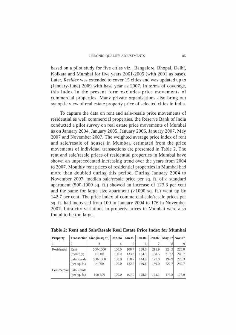
based on a pilot study for five cities viz., Bangalore, Bhopal, Delhi,Kolkata and Mumbai for five years 2001-2005 (with 2001 as base).Later, Residex was extended to cover 15 cities and was updated up to(January-June) 2009 with base year as 2007. In terms of coverage,this index in the present form excludes price movements ofcommercial properties. Many private organisations also bring outsynoptic view of real estate property price of selected cities in India.

To capture the data on rent and sale/resale price movements ofresidential as well commercial properties, the Reserve Bank of Indiaconducted a pilot survey on real estate price movements of Mumbaias on January 2004, January 2005, January 2006, January 2007, May2007 and November 2007. The weighted average price index of rentand sale/resale of houses in Mumbai, estimated from the pricemovements of individual transactions are presented in Table 2. Therent and sale/resale prices of residential properties in Mumbai haveshown an unprecedented increasing trend over the years from 2004to 2007. Monthly rent prices of residential properties in Mumbai hadmore than doubled during this period. During January 2004 toNovember 2007, median sale/resale price per sq. ft. of a standardapartment (500-1000 sq. ft.) showed an increase of 123.3 per centand the same for large size apartment (>1000 sq. ft.) went up by142.7 per cent. The price index of commercial sale/resale prices persq. ft. had increased from 100 in January 2004 to 176 in November2007. Intra-city variations in property prices in Mumbai were alsofound to be too large.

Table 2: Rent and Sale/Resale Real Estate Price Index for Mumbai

Property Transaction Size (in sq. ft.) Jan-04 Jan-05 Jan-06 Jan-07 May-07 Nov-07

1 2 3 4 5 6 7 8 9

Residential Rent 500-1000 100.0 108.7 138.6 211.9 224.3 228.8(monthly) >1000 100.0 133.8 164.9 188.5 219.2 240.7

Sale/Resale 500-1000 100.0 118.7 144.9 177.0 194.9 223.3(per sq. ft.) >1000 100.0 122.2 149.6 189.0 222.7 242.7

Commercial Sale/Resale(per sq. ft.) 100-500 100.0 107.0 128.0 164.1 175.8 175.9


In the present paper, using the same data, we develop the hedonicprice index for residential properties in Mumbai.

Section VI

Estimation and Analysis of Hedonic Regression

As indicated earlier, hedonic regression was estimated based onthe data obtained from the RBI pilot survey conducted in 25 areas ofGreater Mumbai during January 2004-November 2007 covering bothresidential and commercial properties. The actual transaction price,inclusive of land but exclusive of registration fee, stamp duty,brokerage fee, etc., was taken as the purchase price. The selection ofsample in Mumbai was based on the municipal administrative zones.Six urban municipal administrative zones and six municipalitiesconstituted the strata for selection of areas. In all 25 representativeareas with high number of transactions were selected across the 12areas (six zones + six municipalities) on the basis of their share inthe total areas in zones. For proper representation, a total of 20transactions per year in each of the 25 areas were captured. Thus, asample of 500 transactions was collected as on January 2004, January2005, January 2006, January 2007, May 2007 and November 2007.The information for each transaction within a particular area wasclassified according to whether it is a residential property or acommercial property. Within the residential and commercial propertyselected, the transactions were further classified into whether theproperty is used for rental purposes or is subjected to sale/resale inthe time period under consideration.

Six quality attributes associated with price variations areconsidered in the hedonic model. These are: floor (F) in which houseis situated; floor space area (FSA), number of rooms (R), number ofbath rooms (B), whether it is sale or resale (S) and availability of lift(L). Classifications of these attributes are presented in Table 3. Inthe hedonic regression model, all the categories are represented bydummy variables. Apart from these attributes, dummy variables areused to represent separate areas (corresponding to 6 zones in GreaterMumbai, indicated by zone Z1 to Z6, and 6 municipalities,) and 6


time periods (T). The list of the areas under each zone andmunicipality is given in Table D1 in the Annex. As expected, thereexists a large price disparity across zones. For example, the per squarefeet price in Malabar Hill, which comes under the zone 1, is expectedto be much higher than any of the areas in the suburbs. Among thedifferent zones in suburbs also, the house prices are expected to beheterogenous. Results of the hedonic regression method are presentedseparately for time dummy method and characteristics price method.

VI.1 Hedonic Index for Residential Properties: Time Dummy Method

VI.1.1. Rent

For obtaining the hedonic index using this method, the dependentvariable is natural logarithm of per square feet rent. The regressioncoefficients obtained are presented in the Table A of Annex. It can be

Table 3: Quality attributes of selected real estate properties

Sl. No Attribute Category

1 2 3

1. Floors(F) 1 = 0<F<1

2 = 1<F<3

3 = 3<F<5

4 = F>5

2. Floor Space Area (FSA)(in sq. ft.) 1 = 0<FSA=600

2 = 600<FSA<1000

3 = FSA>1000

3. Number of rooms (R) 1 = 1R

2 = 2R

3 = R>3

4. Number of bathrooms (B) 1 = 1B

2 = 2B

3 = B>3

5. Sale or Resale (S) 1= Sale

0 = Resale

6. Availability of lift(L) 1= Lift

0 = No Lift


seen that all zones are having significantly higher rent compared tothe average rent for zone 5. Further the rent of zone 1 is 7.3 times(exp(1.99)) than that of zone 5. Further, higher floors are found tohave more rent, as coefficients corresponding to all floor categoriesare found to be significantly positive. As expected, larger floor spacearea leads to higher rent. The rent of two room houses is notsignificantly different from one room house. This can be viewed asthe number of rooms being insignificant when considered independentof the floor space area. However, for the three room houses, rent issignificantly higher. Rent in case of three bathroom house is alsosignificantly different from one bathroom house.

The quality-adjusted index is calculated directly by taking theexponential of the time-dummy coefficient. The Table 4 gives priceindex for rented residential properties in Greater Mumbai with January2004 as base. The hedonic rent index, taking into account the changesin attributes of residential properties was increasing on an average atthe rate of 20 per cent per annum (Table 4). The index registeredhighest growth during January 2006 - January 2007 of 30.4 per cent.Afterwards, it decelerated. Chart 1 shows the house rent index usingTime Dummy method for different areas of Greater Mumbai.

VI.1.2. Sale/Resale

Regression coefficients obtained are presented in Table B in Annex.Zones 1, 2, and 3 are having significantly higher price compared to the

Table 4: Hedonic Rent Index for Greater Mumbai- Time Dummy Method

Time Period Hedonic Index for Rent Annual Growth Rate(using Time Dummy Method) (in %)

1 2 3

Jan-04 100.0Jan-05 106.2 6.2Jan-06 131.5 23.8Jan-07 171.5 30.4May-07 193.0 12.5 *Nov-07 215.1 25.4 *

* : Over Jan 2007.


average price of zone 6. Further the price of zone 1 is 4.5 times (exp(1.50))than that of zone 6. The zone 4 and zone 6 are found to be have nosignificant difference in their average house price. The price of zone 5 isfound to be significantly lower than that of zone 6. As expected the firsthand sale is priced significantly more than that of resale price. It is foundthat the higher floors are priced significantly more than that of groundfloor. The larger area, as expected, is significantly priced more. It isfound that number of rooms is related negatively to price and it is foundto be significant for more than 3 rooms category. It can viewed as lessprice for more number of rooms for a given floor space area. Table 5shows zone wise hedonic price indices for sale/resale of residential

Table 5: Hedonic Index using Sale/resale prices of ResidentialProperties in Greater Mumbai (Time Dummy Method)

Zones Jan-04 Jan-05 Jan-06 Jan-07 May-07 Nov-07

1 2 3 4 5 6 7

Zone 1 100.0 111.7 154.8 205.8 268.3 311.3Zone 2 100.0 117.4 134.6 165.3 164.6 175.3Zone 3 100.0 124.0 161.8 172.0 202.2 222.9Zone 4 100.0 136.2 158.0 189.8 200.6 208.5Zone 5 100.0 118.2 147.7 179.6 201.6 218.0Zone 6 100.0 119.3 131.8 163.6 163.8 160.5Greater Mumbai 100.0 121.9 147.8 177.5 194.3 209.6


properties using time dummy method. During the four year period, viz.,2004-07, the index grew at an average rate of 18 per cent per annum.The growth rate of the index for zone 1 area was the highest (25 per centper annum) whereas, for zone 6 area, it was the lowest (13 per cent). Forzone 2 to zone 5, the price increase was in the range of 15-19 per centper annum.

Table 6 shows hedonic index of sale/resale prices of residentialproperties in adjacent municipalities of Mumbai using time dummymethod. The average rate of growth of index was highest in Badlapur(40 per cent) whereas it was lowest in Thane (9 per cent). Table C inAnnex presents regression results for adjacent municipalities.

V.2 Hedonic Price Index for Residential Properties: CharacteristicsPrice Index Method

For calculating the index based on the characteristics price indexmethod, we first identified the modal houses for different zones anddifferent time periods. The modal values of the characteristics, viz.,number of bathrooms, rooms, availability of lift, etc., are taken asthe characteristics of the representative modal house in each zonefor different time periods (Table E in Annex). The modal house isthe most frequently transacted attribute of different characteristicsin different zones during a particular period. The price movement ofMumbai city is estimated as the weighted average prices of 6 major

Table 6: Hedonic Index using Sale/resale prices of ResidentialProperties in Adjacent Municipalities of Greater Mumbai

(Time Dummy Method)

Municipalities Jan-04 Jan-05 Jan-06 Jan-07 May-07 Nov-07

1 2 3 4 5 6 7

Navi Mumbai 100.0 138.9 166.1 203.8 210.4 246.9Thane 100.0 111.1 128.3 146.5 213.3 202.1Kalyan 100.0 151.8 180.2 232.2 238.7 240.3Mira Road/ Bhyander 100.0 160.9 227.5 299.8 321.3 310.0Virar/ Vasai 100.0 159.1 241.8 292.4 303.7 337.0Badlapur 100.0 162.7 281.4 338.8 340.7 351.5


tax zones (excluding municipalities), weights being the proportionof house stocks of the tax zones (Table D2 in Annex). The regressioncoefficients obtained are given in Table F of Annex. The relative priceof zone 1, 2 and 3 with respect to zone 6 had been increasing steadilyover the time points considered. This indicates the widening housingprice gap between southern areas of Mumbai and its suburbs. Thecoefficients of zones 4 and 5 which are found to be negative in 2004and 2005 became significantly positive in November 2007. Thisindicates that the price in zone 4 and 5 were less than zone 6 in 2004and 2005, which had appreciated more and overtook zone 6 in 2007.

The Table 7 gives hedonic price index for residential propertiesin Mumbai using characteristics price index method. For residentialproperties of Mumbai using characteristic price index method, theaverage growth rate of index was around 17 per cent annum. Growthrate of house prices was highest for zone 1 areas (27 per cent) whereasit was lowest for zone 6 areas (9 per cent). For other areas of greaterMumbai, the growth rate was in the range of 12-20 per cent.

Table G in Annex gives regression results obtained for adjacentmunicipalities. In contrast to the coefficients of the zones in GreaterMumbai, the coefficients of adjacent municipalities tend to fall. Thisshows that the difference in house prices in the surrounding part ofGreater Mumbai was decreasing. The Table 8 shows the price indexfor residential properties in adjacent municipalities of Mumbai using

Table 7: Hedonic price Index using sale/resale prices of ResidentialProperties in Mumbai - Characteristics Price Index Method

Zones Jan-04 Jan-05 Jan-06 Jan-07 May-07 Nov-07

1 2 3 4 5 6 7

Zone1 100.0 109.9 166.0 215.3 258.1 304.2Zone2 100.0 114.7 126.1 153.1 154.4 157.5Zone3 100.0 120.1 152.8 162.8 187.3 211.8Zone4 100.0 129.6 147.1 199.2 198.9 203.8Zone5 100.0 118.4 140.8 176.2 197.8 219.0Zone6 100.0 118.0 122.5 151.4 161.6 146.3Greater Mumbai 100.0 118.9 142.1 173.7 189.5 202.9


Table 8: Hedonic Index using Sale/resale Prices ofResidential Properties in Adjacent Municipalities -

Characteristics Price Index Method

Municipalities Jan-04 Jan-05 Jan-06 Jan-07 May-07 Nov-07

1 2 3 4 5 6 7

Navi Mumbai 100.0 161.8 245.8 302.6 308.8 301.1

Thane 100.0 161.2 259.3 265.3 317.6 301.1

Kalyan 100.0 214.4 304.0 317.0 337.2 255.1

Mira Road/Bhayander 100.0 170.0 271.7 346.2 325.4 323.0

Virar/Vashi 100.0 170.0 283.7 346.2 345.3 341.0

Badlapur 100.0 171.4 305.5 383.5 359.7 363.4

Characteristics Price Index method. The prices in adjacent areas ofmunicipalities were growing at a higher rate than in the GreaterMumbai area. Growth rate in Badlapur municipality was the highest(44 per cent) whereas it was lowest in Thane (30 per cent).

Chart 2 gives comparison of price indexes obtained from thefour different methods. The hedonic price indices are less as comparedto other indices for the period under consideration. That is, priceincrease is subdued once the effect of quality attribute is controlled.This indicates that in order to asses the price movements of housingsector, quality attribute must be considered. The price indexes for


greater Mumbai obtained from two hedonic methods, viz., timedummy and characteristic price method were moving together till January2007. However, the index obtained from characteristic price method wasmoving slowly as compared to time dummy after January 2007.

Section VII

Conclusion

House is a major form of individual wealth. Understanding itsprice changes is important as changes in its value may influenceconsumer spending and saving decisions, and thus affect overalleconomic activity. From the Central Banks’ point of view, these areparticularly important for maintaining financial stability. While it isimportant to have accurate measure of aggregate housing prices, itsmeasurement poses significant conceptual and practical problems aseach house is associated with many quality attributes which makesprice comparisons difficult across units. Different methodologies havebeen followed to measure aggregate price of housing. This paperattempts to construct hedonic price index by two different methods,viz., Time Dummy Method and Characteristics Price Index methodusing the data on rent and sale/resale prices of residential propertiesin Mumbai for the period from January 2004 to November 2007.Results reveal that the price indices for Greater Mumbai obtainedfrom the above-mentioned two methods were moving together tillJanuary 2007. However, the index obtained from characteristic pricemethod moved slowly as compared to time dummy method afterJanuary 2007. The hedonic price indices are less as compared to otherindices for the period under consideration. That is, price increase issubdued once the effect of quality attribute is controlled. Thisindicates that in order to asses the price movements of housing sector,effect of quality attributes must be considered.


References:

Bascher, J. and Lacroix T. (1999), “Dishwashers and PCs in the FrenchCPI: Hedonic Modelling from Design to Practice”, presented at the Fifthmeeting of the International Working Group on Price Indexes, Reykjavik,Iceland, August, 1999.

Chow, G.C. (1967), “Technological Change and the Demand forComputers”, American Economic Review 57, pp. 1117–1130.

Court, A. (1939), “Hedonic Price Indexes with Automotive Examples”,The Dynamics of Automobile Demand, pp.99-117, General MotorsCorporation.

Diewert W.E. (2001), “Hedonic Regressions: A Consumer TheoryApproach”, Discussion Paper, Department of Economics, University ofBritish Columbia.

Fixler, D., Fortuna, C., Greenlees, J. and Wlater, L . (1999), “The Use ofHedonic Regressions to Handle Quality Change: The Experience in theUS CPI”, paper presented at the Fifth Meeting of the International Workinggroup of Price Indexes, Reykjavik, Iceland, August 1999.

Griliches, Z. (1961), “Hedonic Price Indexes for Automobiles: AnEconometric Analysis of Quality Change”, The Price Statistics of FederalGovernment, New York, National Bureau of Economic Research.

Lancaster, K. (1971), “Consumer Demand: A New Approach”, ColumbiaUniversity Press, New York.

Liegey, P.R. and Shepler, N. (1999), “Adjusting VCR Prices for QualityChange: A Study Using Hedonic Method”, Monthly Labour Review.

Melser, D. (2005), “The Hedonic Regression Time-Dummy Method AndThe Monotonicity Axioms”, Journal of Business & Economic Statistics,23(4): 485-492.

Okamoto, M. and Sato, T. (2001), “Comparison of Hedonic Method andMatched Models Methods using Scanner Data: The Case of PCs, TVs andDigital Cameras”, Paper presented at the Sixth Meeting of the InternationalWorking Group on Price Indexes, Canberra, Australia, 2-6 April 2001.


Pakes, A. (2001), “A Reconsideration of Hedonic Price Indexes with anApplication to PC’s”, NBER working paper 8715, Cambridge MA.

Plosser, C. I. (2007), “House Prices and Monetary Policy”, Speech by thePresident, Federal Reserve Bank of Philadelphia, European Economics andFinancial Centre, Distinguished Speakers Series.

Rosen, S. (1974), “Hedonic Prices and Implicit markets: ProductDifferentiation and Pure Competition”, Journal of Political Economy, 82,34-49.

Shiratsuka, S. (1999), “Asset Price Fluctuation and Price Indices”, Monetaryand Economic Studies.

Sutton, G. (2002), “Explaining Changes in House Prices”, BIS QuarterlyReview.

Triplett, J. E (2001), Handbook on Quality Adjustment of Price Indexesfor Information and Communication Technology Products, Paris: OECD.

Triplett, J.E., and McDonald R.J. (1977), “Assessing the Quality Error inOutput Measures: The Case of Refrigerators”, The Review of Income andWealth, 23, 137-156.

Waugh, Frederick, V. (1928): “Quality Factors Influencing VegetablePrices”, Journal of Farm Economics, 10,185-196.


Figures in parenthesis are SE ; *Significant at 5 per cent level; **Significant at 10 per cent level;

Note : The regression equation is attempted with logarithm of house price as the dependent variable.The coefficients corresponding to the attributes zone 6, time period corresponding to January2004, floor space area in the range 0 to 600 square feet, one bed room house and onebathroom house are set to zero. Thus the coefficients corresponding to other attributes ofthat variable are interpreted in relation to that attribute which is set to zero.

Table B: Regression coefficients –Time Dummy Hedonic for Greater Mumbai – Sale/Resale

Con S L z01 z02 z03 z04 z05 t02 t03 t04

1 2 3 4 5 6 7 8 9 10 11

8.18* 0.40* 0.03 1.50* 0.75* 0.54* 0.00 -0.07* 0.20* 0.39* 0.57*(0.08) (0.04) (0.03) (0.04) (0.03) (0.03) (0.03) (0.03) (0.02) (0.02) (0.02)

t05 t06 f02 f03 f04 a02 a03 r02 r03 b02 b03

12 13 14 15 16 17 18 19 20 21 22

0.66* 0.74* 0.06* 0.09* 0.11* 0.09* 0.15* -0.07 -0.13** 0.03 0.09**(0.02) (0.02) (0.02) (0.02) (0.03) (0.02) (0.03) (0.07) (0.07) (0.04) (0.05)

Annex

Figures in parenthesis are SE; * Significant at 5 per cent level ; **Significant at 10 per cent level;

Note : The regression equation is formulated in a semi-log form with logarithm of house rentas the dependent variable. The data corresponding to zone 6 were very few in number.So those were not taken into account while calculating the rent price index for GreaterMumbai. The coefficients corresponding to the attributes of houses in zone 5 in January2004 with FSA in the range of 0 to 600 sq. ft and having one bedroom and one bathroomhouse are set to zero.

t06 f02 f03 f04 a02 a03 r02 r03 b02 b03

11 12 13 14 15 16 17 18 19 20

0.77* 0.09** 0.14* 0.14* 0.14* 0.33* 0.07 0.29* 0.00 0.32**(0.06) (0.05) (0.06) (0.06) (0.05) (0.09) (0.16) (0.20) (0.10) (0.17)

Table A: Regression coefficients –Time Dummy Hedonic for Greater Mumbai - Rent

Con Lift z01 z02 z03 z04 t02 t03 t04 t05

1 2 3 4 5 6 7 8 9 10

1.98* 0.02 1.99* 0.52* 0.37* 0.16* 0.06 0.27* 0.54* 0.66*(0.2) (0.08) (0.07) (0.07) (0.07) (0.07) (0.05) (0.06) (0.06) (0.05)


Table C : Regression coefficients – Time Dummy Hedonic forGreater Mumbai (Zone-wise) and Adjacent Municipalities- Price

Area Zone Zone Zone Zone Zone Zone Navi Thane Kalyan Mira Virar/ Badla-1 2 3 4 5 6 Mumbai Road/ Vasai pur

Bhaya-nder

1 2 3 4 5 6 7 8 9 10 11 12 13

Con 9.18* 8.55* 8.18* 7.71* 7.35* 8.38* 7.33* 7.01* 7.82* 7.04* 6.93* 5.73*(0.16) (0.13) (0.57) (0.16) (0.26) (0.04) (0.16) (0.45) (0.04) (0.12) (0.05) (0.04)

S @ 0.04 0.07 0.10 0.23 0.52* 0.18* 0.08 0.58* 0.20* 0.36* @(0.11) (0.24) (0.08) (0.14) (0.02) (0.08) (0.11) (0.03) (0.05) (0.03)

L 0.05 0.21* 0.31 0.1* 0.00 0.01 0.05 0.10 0.00 @ -0.03 0.03(0.15) (0.03) (0.47) (0.03) (0.19) (0.02) (0.1) (0.29) (0.03) (0.02) (0.03)

t02 0.11* 0.16* 0.21* 0.31* 0.17* 0.18* 0.34* 0.09 0.42* 0.48* 0.47* 0.49*(0.04) (0.04) (0.1) (0.04) (0.03) (0.02) (0.05) (0.11) (0.02) (0.05) (0.04) (0.03)

t03 0.44* 0.3* 0.48* 0.46* 0.39* 0.28* 0.52 0.25* 0.59 0.82* 0.89* 1.03*(0.05) (0.04) (0.09) (0.04) (0.03) (0.02) (0.04) (0.1) (0.02) (0.05) (0.04) (0.03)

t04 0.72* 0.5* 0.54* 0.64* 0.59* 0.49* 0.72* 0.38* 0.84 1.1* 1.08* 1.22*(0.04) (0.04) (0.09) (0.04) (0.03) (0.02) (0.05) (0.11) (0.02) (0.05) (0.04) (0.03)

t05 0.99* 0.5* 0.7* 0.7* 0.7* 0.49* 0.75* 0.76* 0.87 1.17* 1.11* 1.23*(0.05) (0.04) (0.1) (0.04) (0.03) (0.02) (0.05) (0.11) (0.02) (0.05) (0.04) (0.03)

t06 1.14* 0.56* 0.8* 0.73* 0.78* 0.47* 0.92* 0.7* 0.88 1.13* 1.22* 1.26*(0.04) (0.04) (0.09) (0.04) (0.03) (0.02) (0.05) (0.12) (0.02) (0.05) (0.04) (0.03)

f02 -0.05 0.06 0.28* -0.01 0.00 0.00 0.01 0.07 -0.01 -0.06 0.01 -0.01(0.05) (0.04) (0.09) (0.03) (0.03) (0.01) (0.04) (0.1) (0.01) (0.11) (0.04) (0.02)

f03 0 0.17* 0.17 -0.01 0.01 0 0.01 -0.01 0.00 -0.04 0.02 -0.05(0.05) (0.04) (0.09) (0.04) (0.03) (0.03) (0.05) (0.11) (0.02) (0.11) (0.05) (0.06)

f04 0.01 0.2* 0.18 0.09 0.04 -0.03 0.04 0.11 @ @ 0.08 @(0.04) (-0.05) (0.1) (0.04) (0.04) (0.06) (0.06) (0.12) (0.11)

a02 0.04 0.15* -0.13 0.03 0.00 -0.02 -0.15* 0.13 0.02 -0.03 0.00 0.04(0.06) (0.03) (0.11) (0.04) (0.05) (0.02) (0.07) (0.14) (0.02) (0.03) (0.02) (0.03)

a03 0.12 0.14* -0.04 0.19* -0.01 -0.02 -0.11 0.27 @ @ 0.03 0.01(0.08) (0.08) (0.14) (0.05) (0.06) (0.04) (0.08) (0.19) (0.15) (0.05)

r02 0.04 -0.12* -0.28 0.23 0.14* 0.03 -0.17 0.00 0.01 0.08* -0.03 0.00(0.07) (0.06) (0.15) (0.13) (0.1) (0.04) (0.12) (0.22) (0.03) (0.04) (0.02) (0.03)

r03 @ -0.4* @ 0.12 @ 0.1 0.21 @ @ @ @ @(0.08) (0.13) (0.04) (0.23)

b02 -0.03 0.02 -0.1 0.1* 0.27* -0.05 -0.18 0.14 0.00 -0.06 0.00 -0.05(0.04) (0.05) (0.09) (0.05) (0.1) (0.02) (0.19) (0.17) (0.03) (0.07) (0.04) (0.03)

b03 @ 0 @ 0.09 0.35* @ -0.20 @ @ @ @ @(0.11) (0.07) (0.11) (0.19)

@ Not Estimable due to insufficient data ; Figures in parenthesis are SE; * Significant at 5 per cent level

Note : The regression equations are attempted with logarithm of house price as the dependent variable. The coefficientscorresponding to the attributes of houses in January 2004 with FSA in the range of 0 to 600 sq. ft and having onebedroom and one bathroom house are set to zero in all the regression equations.


Table D1. Distribution of Sample Colonies byAdministrative Zones

Administrative zones Area

Zone 1 (z01) 1. Cuffe Parade2. Malabar Hill

Zone 2 (z02) 3. Lower Parel4. Matunga East5. Mahim West

Zone 3 (z03) 6. Bandra West7. Andheri East8. Oshivara

Zone 4 (z04) 9. Kurla East10. Tungwa/ Chandivali11. Chembur

Zone 5 (z05) 12. Malad13. Borivali/Kandivali14. Dahisar15. Goregoan

Zone 6 (z06) 16. Bhandup17. Mulund

Municipalities

Navi Mumbai (z07) 18. Vashi19. Khargarh Road

Thane (z08) 20. Pokaran Road 1&2

Kalyan (z09) 21. Near Railway Station

Mira Road/Bhyander (z10) 22. Mira Road

Virar/Vasai (z11) 23. Virar24. Nala Sopara

Other Municipalities (z12) 25. Badlapur

Table D2: Housing Stock Distribution

Zone No. of House Holds Population(as per Census-2001)

1 2 3

1 270644 13775782 406519 19604533 513317 24289084 371736 16756795 372291 18671186 351499 1640978


Table E: Modal Houses

Time Zone S L F (floor) A (area) R B(whether (availability (no. of (no. of

sale/ of lift) rooms) bath-resale) rooms)

1 2 3 4 5 6 7 8

Jan-04 1 Sale Lift > 5 F >1000 SF >2R 2B

Jan-04 2 Sale Lift 4-5 F 600-1000 SF 2R 1B

Jan-04 3 Sale Lift 2-3 F 600-1000 SF >2R 2B

Jan-04 4 Sale Lift 2-3 F < 600 SF 2R 1B





Jan-05 3 Sale Lift 2-3 F < 600 SF >2R 2B












Jan-07 3 Sale Lift 2-3 F >1000 SF >2R 2B

Jan-07 4 Sale Lift > 5 F 600-1000 SF >2R 2B



May-07 1 Sale Lift 2-3 F >1000 SF >2R 2B

May-07 2 Sale Lift 2-3 F < 600 SF 2R 1B

May-07 3 Sale Lift 2-3 F >1000 SF >2R 2B

May-07 4 Sale Lift 2-3 F < 600 SF >2R 2B

May-07 5 Sale Lift 2-3 F < 600 SF 2R 1B

May-07 6 Resale Lift 2-3 F 600-1000 SF >2R 1B

Nov-07 1 Sale Lift > 5 F >1000 SF >2R 2B

Nov-07 2 Sale Lift 4-5 F < 600 SF 2R 1B

Nov-07 3 Sale Lift 2-3 F >1000 SF >2R 2B

Nov-07 4 Sale Lift 2-3 F 600-1000 SF >2R 2B

Nov-07 5 Sale Lift 2-3 F < 600 SF >2R 1B

Nov-07 6 Sale Lift 0-1 F 600-1000 SF >2R 2B


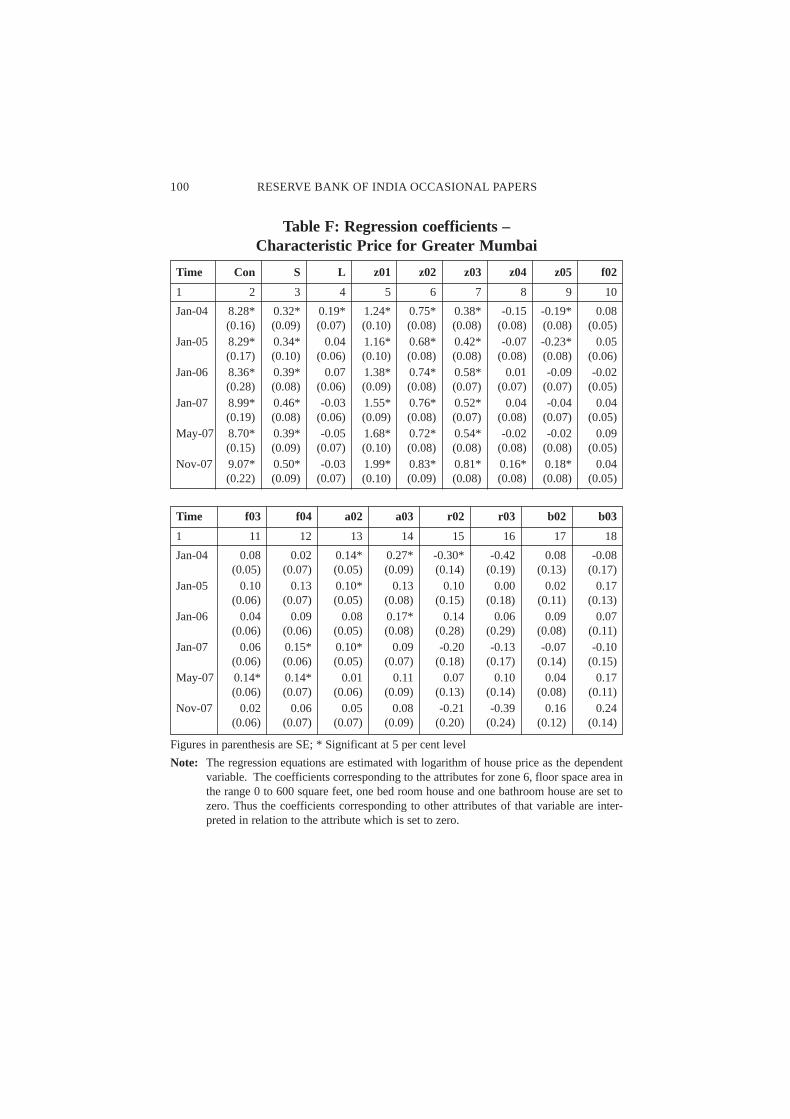
Table F: Regression coefficients –Characteristic Price for Greater Mumbai

Time Con S L z01 z02 z03 z04 z05 f02

1 2 3 4 5 6 7 8 9 10

Jan-04 8.28* 0.32* 0.19* 1.24* 0.75* 0.38* -0.15 -0.19* 0.08(0.16) (0.09) (0.07) (0.10) (0.08) (0.08) (0.08) (0.08) (0.05)

Jan-05 8.29* 0.34* 0.04 1.16* 0.68* 0.42* -0.07 -0.23* 0.05(0.17) (0.10) (0.06) (0.10) (0.08) (0.08) (0.08) (0.08) (0.06)

Jan-06 8.36* 0.39* 0.07 1.38* 0.74* 0.58* 0.01 -0.09 -0.02(0.28) (0.08) (0.06) (0.09) (0.08) (0.07) (0.07) (0.07) (0.05)

Jan-07 8.99* 0.46* -0.03 1.55* 0.76* 0.52* 0.04 -0.04 0.04(0.19) (0.08) (0.06) (0.09) (0.08) (0.07) (0.08) (0.07) (0.05)

May-07 8.70* 0.39* -0.05 1.68* 0.72* 0.54* -0.02 -0.02 0.09(0.15) (0.09) (0.07) (0.10) (0.08) (0.08) (0.08) (0.08) (0.05)

Nov-07 9.07* 0.50* -0.03 1.99* 0.83* 0.81* 0.16* 0.18* 0.04(0.22) (0.09) (0.07) (0.10) (0.09) (0.08) (0.08) (0.08) (0.05)

Time f03 f04 a02 a03 r02 r03 b02 b03

1 11 12 13 14 15 16 17 18

Jan-04 0.08 0.02 0.14* 0.27* -0.30* -0.42 0.08 -0.08(0.05) (0.07) (0.05) (0.09) (0.14) (0.19) (0.13) (0.17)

Jan-05 0.10 0.13 0.10* 0.13 0.10 0.00 0.02 0.17(0.06) (0.07) (0.05) (0.08) (0.15) (0.18) (0.11) (0.13)

Jan-06 0.04 0.09 0.08 0.17* 0.14 0.06 0.09 0.07(0.06) (0.06) (0.05) (0.08) (0.28) (0.29) (0.08) (0.11)

Jan-07 0.06 0.15* 0.10* 0.09 -0.20 -0.13 -0.07 -0.10(0.06) (0.06) (0.05) (0.07) (0.18) (0.17) (0.14) (0.15)

May-07 0.14* 0.14* 0.01 0.11 0.07 0.10 0.04 0.17(0.06) (0.07) (0.06) (0.09) (0.13) (0.14) (0.08) (0.11)

Nov-07 0.02 0.06 0.05 0.08 -0.21 -0.39 0.16 0.24(0.06) (0.07) (0.07) (0.09) (0.20) (0.24) (0.12) (0.14)

Figures in parenthesis are SE; * Significant at 5 per cent level

Note: The regression equations are estimated with logarithm of house price as the dependentvariable. The coefficients corresponding to the attributes for zone 6, floor space area inthe range 0 to 600 square feet, one bed room house and one bathroom house are set tozero. Thus the coefficients corresponding to other attributes of that variable are inter-preted in relation to the attribute which is set to zero.


Table G: Regression coefficients –Characteristic Price for adjacent municipalities

Time cons Sale lift z07 z08 z09 z10 z11 f02

1 2 3 4 5 6 7 8 9 10

Jan-04 5.74* 0.12 0.09 1.62* 1.55* 1.88* 1.10* 0.94* -0.02(0.11) (0.06) (0.06) (0.07) (0.08) (0.10) (0.09) (0.08) (0.05)

Jan-05 6.51* 0.39* 0.11 1.42* 1.11* 1.46* 1.03* 0.80* -0.01(0.09) (0.06) (0.06) (0.08) (0.09) (0.09) (0.09) (0.07) (0.05)

Jan-06 7.08* 0.32* -0.04 1.19* 0.89* 1.33* 0.93* 0.69* 0.02(0.11) (0.09) (0.05) (0.07) (0.07) (0.11) (0.08) (0.07) (0.05)

Jan-07 7.14* 0.21* -0.06 1.22* 0.87* 1.54* 1.04* 0.71* 0.06(0.10) (0.07) (0.05) (0.07) (0.08) (0.11) (0.09) (0.07) (0.05)

May-07 7.19* 0.22* -0.03 1.24* 1.14* 1.52* 1.09* 0.75* -0.05(0.09) (0.06) (0.05) (0.07) (0.08) (0.10) (0.08) (0.07) (0.05)

Nov-07 7.07* 0.06 0.11 1.43* 1.17* 1.70* 1.04* 0.83* 0.05(0.10) (0.06) (0.06) (0.07) (0.08) (0.10) (0.09) (0.07) (0.05)

Time f03 f04 a02 a03 r02 r03 b02 b03

1 11 12 13 14 15 16 17 18

Jan-04 0.02 0.05 -0.07 -0.04 0.07 0.24* -0.03 0.10(0.07) (0.09) (0.04) (0.09) (0.05) (0.12) (0.09) (0.22)

Jan-05 -0.01 -0.05 -0.07 -0.13 0.08 0.14 0.12 0.28(0.06) (0.10) (0.05) (0.11) (0.06) (0.13) (0.09) (0.18)

Jan-06 0.01 0.09 0.02 0.11 -0.03 0.03 -0.02 -0.07(0.06) (0.13) (0.04) (0.10) (0.05) (0.11) (0.08) (0.13)

Jan-07 -0.01 -0.05 0.09* 0.30* -0.08 0.00 -0.06 -0.38*(0.06) (0.09) (0.05) (0.09) (0.06) (0.11) (0.07) (0.11)

May-07 -0.07 0.01 0.00 0.09 0.01 0.05 -0.01 -0.13(0.06) (0.07) (0.04) (0.09) (0.05) (0.10) (0.07) (0.11)

Nov-07 0.06 0.07 0.01 -0.05 -0.07 -0.04 0.00 0.16(0.05) (0.09) (0.05) (0.09) (0.05) (0.10) (0.07) (0.12)

Figures in parenthesis are SE; * Significant at 5 per cent level.

Note: The regression equations are estimated with logarithm of house price as the dependentvariable. The coefficients corresponding to the attributes for Badalapur, floor space areain the range 0 to 600 square feet, one bed room house and one bathroom house are set tozero. Thus the coefficients corresponding to other attributes of that variable are interpretedin relation to the attribute which is set to zero.

Hedonic Quality Adjustments for Real Estate Prices in India · Hedonic Quality Adjustments for Real...

Documents

Transcript of Hedonic Quality Adjustments for Real Estate Prices in India · Hedonic Quality Adjustments for Real...