HEC-RAS MODELING OF RAINBOW RIVER MFL ......SWFWMD TWA# 15TW0000033 HEC-RAS MODELING OF RAINBOW...
90
Submitted by: 1408 North Westshore Boulevard, Suite 115 Tampa, Florida 33607 (813) 289-9338 www.ectinc.com ECT No. 150176-0800-1200 September 25, 2015 SWFWMD TWA# 15TW0000033 HEC-RAS MODELING OF RAINBOW RIVER MFL TECHNICAL SUPPORT – FRESHWATER STREAM FINAL REPORT Submitted to: Southwest Florida Water Management District 2379 Broad Street (U.S. 41 South) Brooksville, FL 34604-6899
Transcript of HEC-RAS MODELING OF RAINBOW RIVER MFL ......SWFWMD TWA# 15TW0000033 HEC-RAS MODELING OF RAINBOW...

Submitted by:
1408 North Westshore Boulevard, Suite 115 Tampa, Florida 33607
(813) 289-9338 www.ectinc.com
ECT No. 150176-0800-1200
September 25, 2015
SWFWMD TWA# 15TW0000033
HEC-RAS MODELING OF RAINBOW RIVER MFL TECHNICAL SUPPORT – FRESHWATER STREAM
FINAL REPORT
Submitted to:
Southwest Florida Water Management District 2379 Broad Street (U.S. 41 South)
Brooksville, FL 34604-6899

SWFWMD TWA# 15TW0000033
HEC-RAS MODELING OF RAINBOW RIVERMFL TECHNICAL SUPPORT - FRESHWATER STREAM
FINAL REPORT
Prepared for:
Southwest Florida Water Management District2379 Broad Street (U.S. 41 South)Brooksville, Florida 34604-6899
Prepared by:
Environmental Consulting & Technology, Inc.1408 North Westshore BoulevardSuite 115Tampa, Florida 33607
Engineer
September 25, 2015

HEC-RAS Modeling of Rainbow River MFL Technical Support – Freshwater Streams (TWA 15TW0000033) Final Report
i P:\S2300_SWFWMD\150176_Rainbow River\5-Reports\Task_8_Final_Report\Rainbow_Final Report_20150925.docx
TABLE OF CONTENTS 1. INTRODUCTION ........................................................................................ 1-1 1.1 Background ...................................................................................................................................... 1-1 1.2 Project Study Area........................................................................................................................... 1-1 2. HEC-RAS MODEL DEVELOPMENT ......................................................... 2-1 2.1 Geometric Data Development in HEC-GeoRAS ........................................................................... 2-1
2.1.1 River Centerline ....................................................................................................................... 2-1 2.1.2 Cross-Section Cutlines ............................................................................................................. 2-1 2.1.3 Bridges ..................................................................................................................................... 2-3 2.1.4 Optional GIS Layers ................................................................................................................. 2-3
2.2 Geometric Data Development in HEC-RAS .................................................................................. 2-4 2.2.1 Cross-Sections .......................................................................................................................... 2-5 2.2.2 Bridges ..................................................................................................................................... 2-6
2.3 Preliminary HEC-RAS Model Simulation .................................................................................... 2-7 2.3.1 Channel Flow Profiles .............................................................................................................. 2-7 2.3.2 Downstream Boundary Conditions ........................................................................................ 2-11 2.3.3 Steady-State Model Simulation .............................................................................................. 2-14
3. HEC-RAS MODEL CALIBRATION ........................................................... 3-1 3.1 Gage Data Analysis .......................................................................................................................... 3-1 3.2 Dynamic Flow Data – Boundary Conditions ................................................................................. 3-6
3.2.1 Flow Hydrograph Boundary Conditions .................................................................................. 3-6 3.2.2 Stage Hydrograph Boundary Conditions .................................................................................. 3-7 3.2.3 Lateral Inflow Hydrograph Boundary Conditions .................................................................... 3-8
3.3 Dynamic HEC-RAS Model Simulation and Calibration ............................................................ 3-10 3.3.1 Model Simulation ................................................................................................................... 3-10 3.3.2 Model Stabilization ................................................................................................................ 3-10 3.3.3 Model Calibration .................................................................................................................. 3-11 3.3.4 Model Verification ................................................................................................................. 3-30
3.4 Summary of Dynamic HEC-RAS Model Calibration ................................................................. 3-33 4. MFL SCENARIO SIMULATIONS .............................................................. 4-1 4.1 Steady-State Model Parameterization ........................................................................................... 4-1
4.1.1 USGS Stream-Gauging Stations .............................................................................................. 4-1 4.1.2 Steady-State Flow Scenarios .................................................................................................... 4-1 4.1.3 Channel Flow Profiles .............................................................................................................. 4-4 4.1.4 Downstream Boundary Conditions .......................................................................................... 4-4
4.2 Steady-State Model Simulation ...................................................................................................... 4-8 4.2.1 Model Simulation ..................................................................................................................... 4-8 4.2.2 Simulation Results.................................................................................................................... 4-8
4.3 Steady-State Model Verification ................................................................................................... 4-14 4.3.1 Model Verification Targets .................................................................................................... 4-14 4.3.2 Model Verification Results .................................................................................................... 4-14
4.4 Summary of MFL Scenario Simulations ..................................................................................... 4-17 5. CONCLUSIONS AND RECOMMENDATIONS .......................................... 5-1 6. REFERENCES ........................................................................................... 6-1

HEC-RAS Modeling of Rainbow River MFL Technical Support – Freshwater Streams (TWA 15TW0000033) Final Report
ii P:\S2300_SWFWMD\150176_Rainbow River\5-Reports\Task_8_Final_Report\Rainbow_Final Report_20150925.docx
TABLE OF CONTENTS (Continued, Page 2 of 2)
LIST OF APPENDICES APPENDIX A - REFERENCES ON HYDRAULIC PARAMETERS APPENDIX B - HEC-RAS MODEL INPUT & OUTPUT DATA (Located on CD)

HEC-RAS Modeling of Rainbow River MFL Technical Support – Freshwater Streams (TWA 15TW0000033) Final Report
iii P:\S2300_SWFWMD\150176_Rainbow River\5-Reports\Task_8_Final_Report\Rainbow_Final Report_20150925.docx
LIST OF TABLES
Table 2–1. Summary of Data Sources for Cross-Section Characterization ..................... 2-3 Table 2–2. Summary of Flow Distribution Analysis Results ........................................ 2-10 Table 2–3. Summary of Channel Flow Profile .............................................................. 2-10 Table 3–1. Summary of Stage Datasets in Rainbow and Withlacoochee Rivers ............ 3-3 Table 3–2 Summary of Lateral/Uniform Lateral Inflow Hydrograph Boundary
Conditions ...................................................................................................... 3-9 Table 3–3. Summary of Calibration Targets for Model Calibration.............................. 3-11 Table 3–4. Summary of Flow Roughness Factors in Cross-Sections (RS 3.11 - 6.00) . 3-12 Table 3–5. Summary of Model Calibration Results ...................................................... 3-13 Table 3–6. Summary of Stage Datasets Used in Model Verification ............................ 3-31 Table 4–1. Summary of Flow Impact Factors at USGS 02313100 ................................. 4-2 Table 4–2. Summary of Selected Steady-State Flow Scenarios at USGS 02313100 ...... 4-3 Table 4–3. Summary of Selected Steady-State Stage Scenarios at USGS 02313200 ..... 4-6 Table 4–4. Summary of Downstream Boundary Conditions – Stages at USGS 02313100
Using Multiple Regression Curve .................................................................. 4-7 Table 4–5. Summary of Model Verification Targets - Simple Linear Regression Curve 4-16 Table 4–6. Summary of Model Verification Targets - Multiple Regression Curve ..... 4-18 Table 4–7. Summary of Model Simulation Results – Stage at Spring Head (RS 6.00) 4-19
HEC-RAS Modeling of Rainbow River MFL Technical Support – Freshwater Streams (TWA 15TW0000033) Final Report
iv P:\S2300_SWFWMD\150176_Rainbow River\5-Reports\Task_8_Final_Report\Rainbow_Final Report_20150925.docx
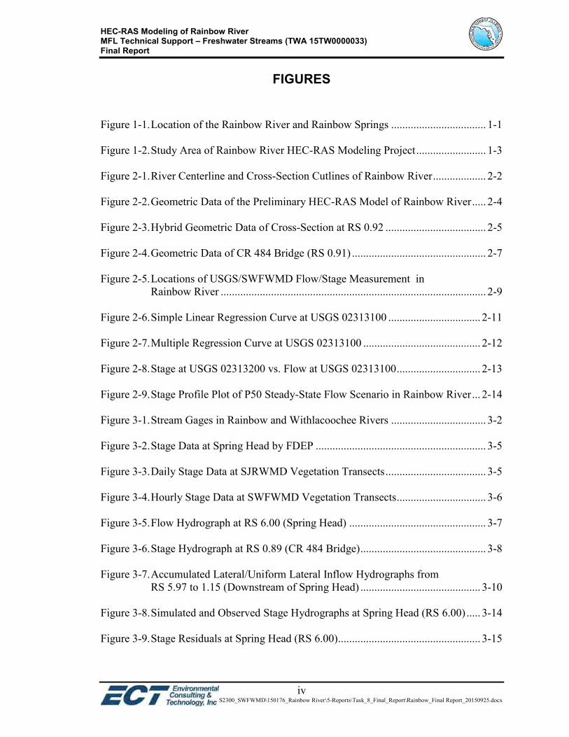
FIGURES
Figure 1-1. Location of the Rainbow River and Rainbow Springs .................................. 1-1 Figure 1-2. Study Area of Rainbow River HEC-RAS Modeling Project ......................... 1-3 Figure 2-1. River Centerline and Cross-Section Cutlines of Rainbow River ................... 2-2 Figure 2-2. Geometric Data of the Preliminary HEC-RAS Model of Rainbow River ..... 2-4 Figure 2-3. Hybrid Geometric Data of Cross-Section at RS 0.92 .................................... 2-5 Figure 2-4. Geometric Data of CR 484 Bridge (RS 0.91) ................................................ 2-7 Figure 2-5. Locations of USGS/SWFWMD Flow/Stage Measurement in Rainbow River ............................................................................................... 2-9 Figure 2-6. Simple Linear Regression Curve at USGS 02313100 ................................. 2-11 Figure 2-7. Multiple Regression Curve at USGS 02313100 .......................................... 2-12 Figure 2-8. Stage at USGS 02313200 vs. Flow at USGS 02313100 .............................. 2-13 Figure 2-9. Stage Profile Plot of P50 Steady-State Flow Scenario in Rainbow River ... 2-14 Figure 3-1. Stream Gages in Rainbow and Withlacoochee Rivers .................................. 3-2 Figure 3-2. Stage Data at Spring Head by FDEP ............................................................. 3-5 Figure 3-3. Daily Stage Data at SJRWMD Vegetation Transects .................................... 3-5 Figure 3-4. Hourly Stage Data at SWFWMD Vegetation Transects ................................ 3-6 Figure 3-5. Flow Hydrograph at RS 6.00 (Spring Head) ................................................. 3-7 Figure 3-6. Stage Hydrograph at RS 0.89 (CR 484 Bridge) ............................................. 3-8 Figure 3-7. Accumulated Lateral/Uniform Lateral Inflow Hydrographs from RS 5.97 to 1.15 (Downstream of Spring Head) ........................................... 3-10 Figure 3-8. Simulated and Observed Stage Hydrographs at Spring Head (RS 6.00) ..... 3-14 Figure 3-9. Stage Residuals at Spring Head (RS 6.00)................................................... 3-15

HEC-RAS Modeling of Rainbow River MFL Technical Support – Freshwater Streams (TWA 15TW0000033) Final Report
v P:\S2300_SWFWMD\150176_Rainbow River\5-Reports\Task_8_Final_Report\Rainbow_Final Report_20150925.docx
FIGURES (Continued, Page 2 of 4)
Figure 3-10. Scatter Plot Comparing Simulated and Observed Stages at Spring Head
(RS 6.00) ...................................................................................................... 3-15 Figure 3-11. Scatter Plot Comparing Stage Residuals and Observed Stages at Spring
Head (RS 6.00)............................................................................................. 3-16 Figure 3-12. Simulated and Observed Stage Hydrographs at SJR T4 (RS 5.77) ...... 3-16 Figure 3-13. Stage Residuals at SJR T4 (RS 5.77) ..................................................... 3-17 Figure 3-14. Scatter Plot Comparing Simulated and Observed Stages at SJR T4 (RS
5.77) ............................................................................................................. 3-17 Figure 3-15. Scatter Plot Comparing Stage Residuals and Observed Stages at SJR T4
(RS 5.77) ...................................................................................................... 3-18 Figure 3-16. Simulated and Observed Stage Hydrographs at SJR T3 (RS 4.31) ....... 3-18 Figure 3-17. Stage Residuals at SJR T3 (RS 4.31) ..................................................... 3-19 Figure 3-18. Scatter Plot Comparing Simulated and Observed Stages at SJR T3 (RS
4.31) ............................................................................................................. 3-19 Figure 3-19. Scatter Plot Comparing Stage Residuals and Observed Stages at SJR T3
(RS 4.31) ...................................................................................................... 3-20 Figure 3-20. Simulated and Observed Stage Hydrographs at SJR T2 (RS 3.09) ....... 3-20 Figure 3-21. Stage Residuals at SJR T2 (RS 3.09) ..................................................... 3-21 Figure 3-22. Scatter Plot Comparing Simulated and Observed Stages at SJR T2 (RS
3.09) ............................................................................................................. 3-21 Figure 3-23. Scatter Plot Comparing Stage Residuals and Observed Stages at SJR T2
(RS 3.09) ...................................................................................................... 3-22 Figure 3-24. Simulated and Observed Stage Hydrographs at SJR T1 (RS 1.97) ....... 3-22 Figure 3-25. Stage Residuals at SJR T1 (RS 1.97) ..................................................... 3-23 Figure 3-26. Scatter Plot Comparing Simulated and Observed Stages at SJR T1 (RS
1.97) ............................................................................................................. 3-23

HEC-RAS Modeling of Rainbow River MFL Technical Support – Freshwater Streams (TWA 15TW0000033) Final Report
vi P:\S2300_SWFWMD\150176_Rainbow River\5-Reports\Task_8_Final_Report\Rainbow_Final Report_20150925.docx
FIGURES (Continued, Page 3 of 4)
Figure 3-27. Scatter Plot Comparing Stage Residuals and Observed Stages at SJR T1
(RS 1.97) ...................................................................................................... 3-24 Figure 3-28. Simulated and Observed Stage Hydrographs at Veg 7 (RS 5.77) ......... 3-24 Figure 3-29. Stage Residuals at Veg 7 (RS 5.77) ....................................................... 3-25 Figure 3-30. Scatter Plot Comparing Simulated and Observed Stages at Veg 7 (RS
5.77) ............................................................................................................. 3-25 Figure 3-31. Scatter Plot Comparing Stage Residuals and Observed Stages at Veg 7
(RS 5.77) ...................................................................................................... 3-26 Figure 3-32. Simulated and Observed Stage Hydrographs at PHAB 2 (RS 3.09) .... 3-26 Figure 3-33. Stage Residuals at PHAB 2 (RS 3.09) ................................................... 3-27 Figure 3-34. Scatter Plot Comparing Simulated and Observed Stages at PHAB 2 (RS
3.09) ............................................................................................................. 3-27 Figure 3-35. Scatter Plot Comparing Stage Residuals and Observed Stages at PHAB 2
(RS 3.09) ...................................................................................................... 3-28 Figure 3-36. Simulated and Observed Stage Hydrographs at Veg 1 (RS 1.36) ......... 3-28 Figure 3-37. Stage Residuals at Veg 1 (RS 1.36) ....................................................... 3-29 Figure 3-38. Scatter Plot Comparing Simulated and Observed Stages at Veg 1 (RS
1.36) ............................................................................................................. 3-29 Figure 3-39. Scatter Plot Comparing Stage Residuals and Observed Stages at Veg 1
(RS 1.36) ...................................................................................................... 3-30 Figure 3-40. Simulated Stage Hydrographs and Observed Stage Data at Spring Head,
PHAB 1, PHAB Pool & PHAB 2 ................................................................ 3-31 Figure 3-41. Simulated Stage Hydrographs and Observed Stage Data at Veg 7, Veg 4
& Veg 2 ........................................................................................................ 3-32 Figure 3-42. Simulated Stage Hydrographs and Observed Stage Data at Veg 6, Veg 3
& Veg 1 ........................................................................................................ 3-32

HEC-RAS Modeling of Rainbow River MFL Technical Support – Freshwater Streams (TWA 15TW0000033) Final Report
vii P:\S2300_SWFWMD\150176_Rainbow River\5-Reports\Task_8_Final_Report\Rainbow_Final Report_20150925.docx
FIGURES (Continued, Page 4 of 4)
Figure 3-43. Simulated Stage Hydrographs and Observed Stage Data at Veg 2.5 & Veg
BBP .............................................................................................................. 3-33 Figure 4-1. Baseline Flow Data at USGS 02313100 ........................................................ 4-2 Figure 4-2. Flow-Duration Curve of Baseline Flow Data at USGS 02313100 ................ 4-3 Figure 4-3. Historic Stage Data at USGS 02313200 ........................................................ 4-5 Figure 4-4. Stage-Duration Curve at USGS 02313200 .................................................... 4-5 Figure 4-5. Stage Profile Plot of 15 Flow Scenarios in Rainbow River with P50 Stage
Scenario (S10) in Withlacoochee River ....................................................... 4-10 Figure 4-6. Stage Profile Plot of 15 Stage Scenarios in Withlacoochee River with P50
Flow Scenario (F9) in Rainbow River ......................................................... 4-11 Figure 4-7. Cross-Section Plot at Veg 1 (RS 1.36) for P50 Flow Scenario (F9) in Rainbow
River and P50 Stage Scenario (S10) in Withlacoochee River ..................... 4-12 Figure 4-8. Profile Output Table for Steady-State HEC-RAS Model Output Review ... 4-12 Figure 4-9. Stage-Flow Rating Curves at Veg 1 (RS 1.36) ............................................ 4-13 Figure 4-10. Stage-Flow Rating Curves at PHAB 1 (RS 4.96) .................................. 4-13 Figure 4-11. Multiple Regression Curve at Spring Head (RS 6.00) ........................... 4-15 Figure 4-12. Simple Linear Regression Curve at Spring Head (RS 6.00) .................. 4-16 Figure 4-13. Stage Residuals at Spring Head (RS 6.00) Using Multiple Regression
Curve ............................................................................................................ 4-20 Figure 4-14. Stage Residuals at Spring Head (RS 6.00) Using Simple Linear
Regression Curve ......................................................................................... 4-21

HEC-RAS Modeling of Rainbow River MFL Technical Support – Freshwater Streams (TWA 15TW0000033) Final Report
1-1 P:\S2300_SWFWMD\150176_Rainbow River\5-Reports\Task_8_Final_Report\Rainbow_Final Report_20150925.docx
1. INTRODUCTION
1.1 BACKGROUND
Environmental Consulting & Technology, Inc. (ECT) was authorized by the Southwest
Florida Water Management District (SWFWMD or the District) to conduct HEC-RAS
modeling in support of establishing Minimal Flows and Levels (MFLs) for Rainbow
River (the River).
1.2 PROJECT STUDY AREA
The Rainbow River is located in western Marion County, 120 kilometers (75 miles) north
of Tampa and 32 kilometers (20 miles) southeast of Ocala, near the town of Dunnellon
(Figure 1-1). The Rainbow River watershed is approximately 73.5 square miles or 47,000
acres. Land use is primarily urban on the western side of the River and wetland and
upland forest on the eastern side (SWFWMD, 2004). The River starts at Rainbow Springs
and empties into the Withlacoochee River 9.2 kilometers (5.7 miles) to the south of the
headsprings. The Withlacoochee River flows westward into Lake Rousseau, past the
Inglis Dam, and eventually into the Gulf of Mexico.
Figure 1-1. Location of the Rainbow River and Rainbow Springs

HEC-RAS Modeling of Rainbow River MFL Technical Support – Freshwater Streams (TWA 15TW0000033) Final Report
1-2 P:\S2300_SWFWMD\150176_Rainbow River\5-Reports\Task_8_Final_Report\Rainbow_Final Report_20150925.docx
The project study area is selected at the upstream portion of the River, a river segment of
approximately 5.1 river miles in length that is defined by the springhead to the north and
CR 484 Bridge to the south, as graphically presented in Figure 1-2. The overall length of
the River is approximately 6.0 river miles measured from the springhead to its confluence
at Withlacoochee River to the south.
Of the 33 first magnitude springs in the State of Florida, Rainbow Springs, forming the
headwaters of the Rainbow River, is the fourth largest in terms of discharge. The
Rainbow River discharges an average of 763 cubic feet per second (CFS), or 493 million
gallons of water per day (MGD) into the Withlacoochee River, just upstream of Lake
Rousseau. Because of the Rainbow River's exceptional scenic beauty and its ecological
significance, the river has been designated by the State, to be an Outstanding Florida
Water (OFW), an Aquatic Preserve, and a SWIM priority water body (SWFWMD,
2004b).
A staff gage operated by the Florida Department of Environmental Protection (FDEP) is
located just downstream of the springhead, which is the upstream end of the study area.
U.S. Geological Survey (USGS) 02313098 Rainbow River near Dunnellon, Florida, a
short-term stream gage, was recently installed upstream of a rocky shoal in 2013. USGS
02313100 Rainbow River at Dunnellon, Florida, a long-term stream gage that was
installed at the downstream side of CR 484 Bridge, is used to define the downstream
boundary conditions of the HEC-RAS model to be developed in this task.
A long-term USGS groundwater well station, named as USGS 290514082270701
Rainbow Springs Well near Dunnellon, Florida, is located on the east side of U.S.
Highway 41, approximately 2.8 miles north of Dunnellon, Florida. The well records are
used to determine flow of the River at CR 484 Bridge by USGS (Lambeth, D., 2010). A
long-term USGS stream gage at the Withlacoochee River, identified as USGS 02313200
Withlacoochee River at Dunnellon, Florida, is located near center of span on the
downstream side of bridge on U.S. Highway 41, approximately 0.6 mile downstream
from the River. Severe backwater effects are concluded by comparing the stage records

HEC-RAS Modeling of Rainbow River MFL Technical Support – Freshwater Streams (TWA 15TW0000033) Final Report
1-3 P:\S2300_SWFWMD\150176_Rainbow River\5-Reports\Task_8_Final_Report\Rainbow_Final Report_20150925.docx
collected at this USGS gages and USGS gage 02313100 in the River. Locations of
USGS and FDEP gage stations described above are presented in Figure 1-2.
Figure 1-2. Study Area of Rainbow River HEC-RAS Modeling Project

HEC-RAS Modeling of Rainbow River MFL Technical Support – Freshwater Streams (TWA 15TW0000033) Final Report
2-1 P:\S2300_SWFWMD\150176_Rainbow River\5-Reports\Task_8_Final_Report\Rainbow_Final Report_20150925.docx
2. HEC-RAS MODEL DEVELOPMENT
2.1 GEOMETRIC DATA DEVELOPMENT IN HEC-GEORAS
HEC-GeoRAS 4.2.92, an ArcGIS 9.2 extension for HEC-RAS, was used in developing
the HEC-GeoRAS database of the River. A geometry exchange file was created by
HEC-GeoRAS prior to being imported into the new HEC-RAS model.
2.1.1 RIVER CENTERLINE
The river centerline of the River, as shown in Figure 2-1, was provided by SWFWMD for
the river segment within the project study area, from the spring head to CR 484 Bridge.
The river centerline between CR 484 Bridge and the confluence at the Withlacoochee
River was derived from the high-resolution USGS National Hydrography Dataset (NHD),
which was generally developed at a scale of 1:24,000 or 1:12,000.
The river centerline was used to assign the river station (RS) values of the cross-sections,
measured in river miles from the river confluence at the Withlacoochee River along the
river reach, by utilizing HEC-GeoRAS in ArcGIS.
2.1.2 CROSS-SECTION CUTLINES
The primary data source used in characterizing cross-sections in the study area is the
cross-section dataset provided by Dr. Xinjian Chen of SWFWMD, which includes a total
of 165 cross-sections in the project study area.
The secondary data sources include: 1) the 2008 vegetation transect survey performed by
SWFWMD and St. Johns River Water Management District (SJRWMD), including a
total of 12 cross-sections; 2) the 2014 topographic survey of CR 484 Bridge performed
by SWFWMD; and 3) the 2003 Light Detection and Ranging (LiDAR) topographic
survey by SWFWMD in Marion County, as summarized in Table 2-1.
As listed in Table 2-1, a total of 196 raw cross-sections were either provided or derived
from the survey data sources. Based on these raw cross-sections, a total of 179 cross-

HEC-RAS Modeling of Rainbow River MFL Technical Support – Freshwater Streams (TWA 15TW0000033) Final Report
2-2 P:\S2300_SWFWMD\150176_Rainbow River\5-Reports\Task_8_Final_Report\Rainbow_Final Report_20150925.docx
sections, with river stations ranged from 0.89 to 6.00, were digitized and stored in the
HEC-GeoRAS geodatabase, as shown in Figure 2-1, which includes 164 of 165 cross-
sections from 2015 Cross-Section Dataset, 12 of 14 from 2008 Vegetation Transect
Survey, and 3 of 5 from 2014 Topo Survey at CR 484 Bridge.
Figure 2-1. River Centerline and Cross-Section Cutlines of Rainbow River

HEC-RAS Modeling of Rainbow River MFL Technical Support – Freshwater Streams (TWA 15TW0000033) Final Report
2-3 P:\S2300_SWFWMD\150176_Rainbow River\5-Reports\Task_8_Final_Report\Rainbow_Final Report_20150925.docx
Table 2–1. Summary of Data Sources for Cross-Section Characterization
Data Source Name Provider Cross-Section No.
Description
2003 LiDAR DEM SWFWMD - In Marion County, Florida. Used in developing cross-section geometry data in floodplain area.
2008 Bathymetry Survey
SWFWMD/Jones
Edmunds 14
ArcGIS geodatabase point feature (X, Y, Z). Not involved in Geometric Data Development in HEC-GeoRAS as this dataset does not provide additional benefits after compared with the 2015 Cross-Section Dataset.
2008 Vegetation Transect Survey
SWFWMD/ SJRWMD 12
11 Veg Transects by SWFWMD in ESR Shapefile format. 4 Veg Transect by SJRWMD in MS Excel Table (X, Y, Z).
2014 Topo Survey SWFWMD 5 Provided in MS Excel Table (X, Y, Z). For CR 484 bridge.
2015 Cross-Section Dataset
SWFWMD (Dr. Chen) 165
Provided in MS Excel Table (X, Y, Z). Cross-sections at a 164-foot interval A FORTRAN code was developed by Dr. Chen to calculate cross-section geometry data on the basis of 2015 bathymetry survey provided by University of South Florida (USF) and 2003 LiDAR DEM data by SWFWMD.
2.1.3 BRIDGES
Only one bridge centerline was digitized at CR 484 Bridge and stored in the HEC-
GeoRAS geodatabase.
2.1.4 OPTIONAL GIS LAYERS
Optional GIS layers, including flow path and bank line polylines, were also digitized in
support of developing the required cross-section geometric parameters, such as river
stations, downstream reach lengths, bank stations, and others.
With the required and optional GIS layers, a HEC-GeoRAS geodatabase was developed
for the River, including the station-elevation data pairs for all the 179 cross-sections.
A geometry exchange file was then generated by HEC-GeoRAS for future use in HEC-
RAS. The projection coordination system of the geometric data was geo-referenced to
“NAD_1983_HARN_StatePlane_Florida_West_FIPS_0902_Feet.”
HEC-RAS Modeling of Rainbow River MFL Technical Support – Freshwater Streams (TWA 15TW0000033) Final Report
2-4 P:\S2300_SWFWMD\150176_Rainbow River\5-Reports\Task_8_Final_Report\Rainbow_Final Report_20150925.docx
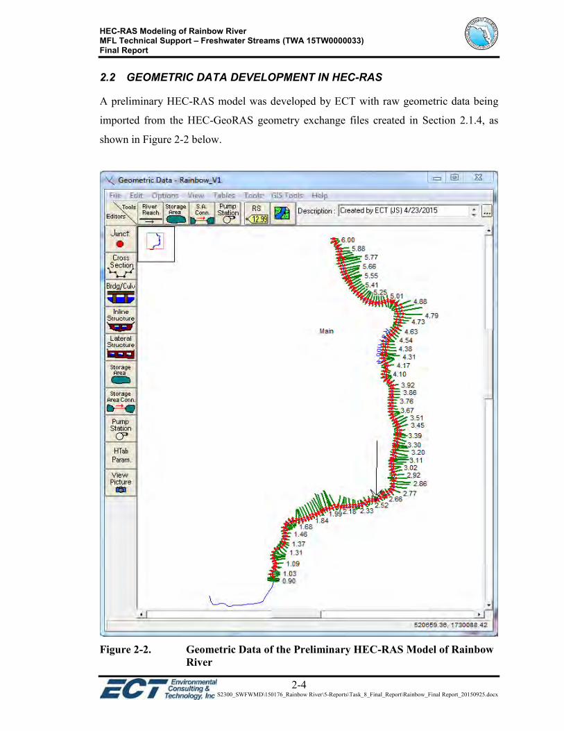
2.2 GEOMETRIC DATA DEVELOPMENT IN HEC-RAS
A preliminary HEC-RAS model was developed by ECT with raw geometric data being
imported from the HEC-GeoRAS geometry exchange files created in Section 2.1.4, as
shown in Figure 2-2 below.
Figure 2-2. Geometric Data of the Preliminary HEC-RAS Model of Rainbow
River

HEC-RAS Modeling of Rainbow River MFL Technical Support – Freshwater Streams (TWA 15TW0000033) Final Report
2-5 P:\S2300_SWFWMD\150176_Rainbow River\5-Reports\Task_8_Final_Report\Rainbow_Final Report_20150925.docx
2.2.1 CROSS-SECTIONS
As part of the HEC-GeoRAS geometry exchange files, the station-elevation data for the
179 cross-sections was derived from the 2003 LiDAR-based DEM data. Given that the
LiDAR-based DEM data is not appropriate to represent the river bathymetry in main
channel, the station-elevation data derived from the survey data sources as listed in Table
2-1 was employed to substitute the main channel portion of the LiDAR-based cross-
section geometric data, for example the cross-section at RS 0.92 as presented in Figure 2-
3 below.
The “hybrid” cross-section geometric data was reviewed by ECT staff, with some minor
adjustments of station-elevation data points and other parameters, such as bank stations
and ineffective flow areas.
Figure 2-3. Hybrid Geometric Data of Cross-Section at RS 0.92
2.2.1.1 Manning’s N Value
Parameterization of Manning’s roughness coefficient (n) is critical to the accuracy of the
simulated water surface levels in hydraulic modeling. The Manning’s n value varies
depending on surface roughness, vegetation, channel irregularities, channel alignment,
2003 LiDAR-based DEM 2003 LiDAR-based DEM 2014 Topo Survey

HEC-RAS Modeling of Rainbow River MFL Technical Support – Freshwater Streams (TWA 15TW0000033) Final Report
2-6 P:\S2300_SWFWMD\150176_Rainbow River\5-Reports\Task_8_Final_Report\Rainbow_Final Report_20150925.docx
scour and deposition, obstructions, size and shape of the channel, stage and discharge,
seasonal changes, temperature, and suspended material and bedload.
The initial values of Manning’s n were assigned with the values used in the existing
HEC-RAS model developed by SWFWMD in 2008. The Manning’s n values were
further adjusted in the subsequent model calibration task, in which the natural conditions
of the main channel and floodplain of the River were reevaluated for modification of the
Manning’s n values for each cross-section, with the assistance of aerial map, land use
map, field observations performed under Task 2, as well as analyses of model results of
calibration runs conducted under Task 5 in this project.
2.2.1.2 Contraction & Expansion Coefficients
The subcritical flow regime is used for steady state flow simulation in the HEC-RAS
modeling. Within the selected study area of the River, the change in effective cross-
section area is not abrupt. Therefore, the expansion and contraction coefficients of 0.1
and 0.3 were applied to most of the 179 cross-sections, except at the cross-sections near
CR 484 Bridge, where expansion and contraction coefficients of 0.3 and 0.5 were
assigned, respectively.
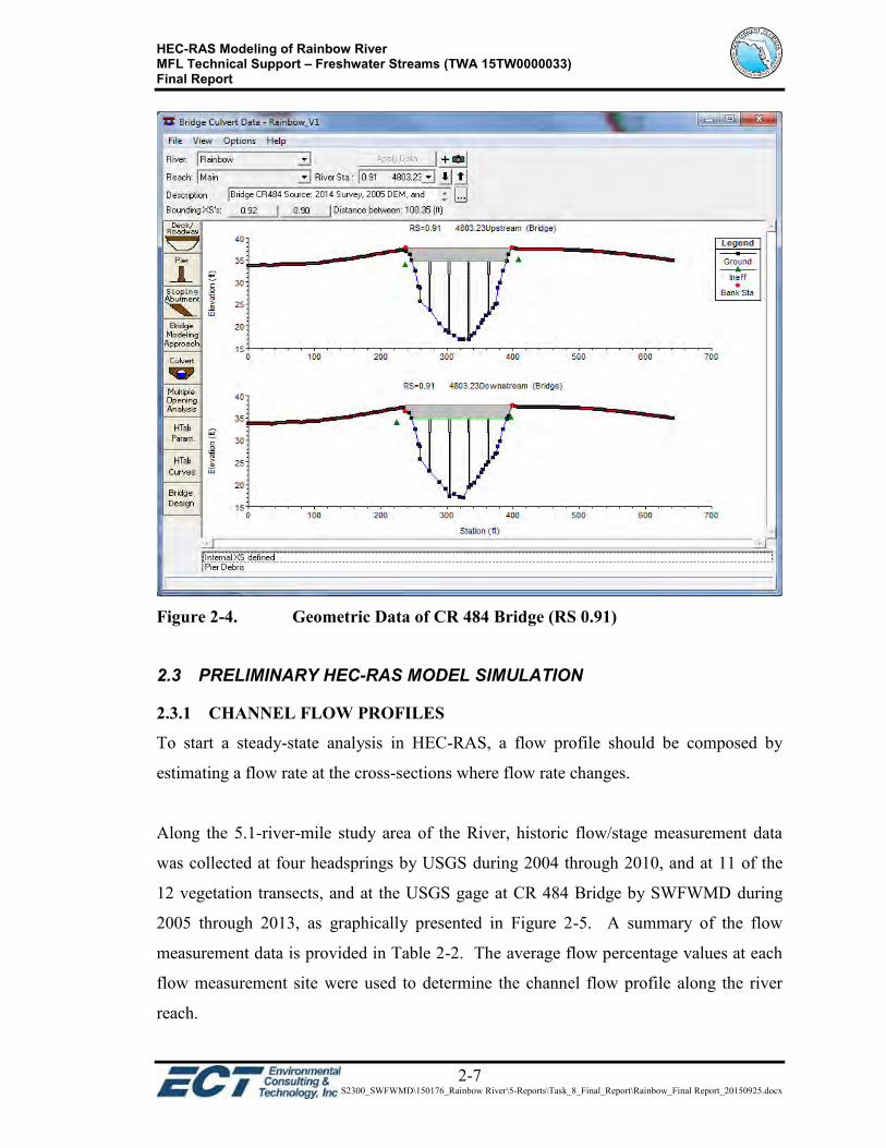
2.2.2 BRIDGES
For the only bridge (CR 484) included in the HEC-RAS model, as shown in Figure 2-4
the geometric data of roadway/deck and piers was mostly derived from the 2014 Topo
Survey data and supplemented with the 2003 LiDAR-based DEM data for the roadway
(Table 2-1).
HEC-RAS Modeling of Rainbow River MFL Technical Support – Freshwater Streams (TWA 15TW0000033) Final Report
2-7 P:\S2300_SWFWMD\150176_Rainbow River\5-Reports\Task_8_Final_Report\Rainbow_Final Report_20150925.docx
Figure 2-4. Geometric Data of CR 484 Bridge (RS 0.91)
2.3 PRELIMINARY HEC-RAS MODEL SIMULATION
2.3.1 CHANNEL FLOW PROFILES
To start a steady-state analysis in HEC-RAS, a flow profile should be composed by
estimating a flow rate at the cross-sections where flow rate changes.
Along the 5.1-river-mile study area of the River, historic flow/stage measurement data
was collected at four headsprings by USGS during 2004 through 2010, and at 11 of the
12 vegetation transects, and at the USGS gage at CR 484 Bridge by SWFWMD during
2005 through 2013, as graphically presented in Figure 2-5. A summary of the flow
measurement data is provided in Table 2-2. The average flow percentage values at each
flow measurement site were used to determine the channel flow profile along the river
reach.

HEC-RAS Modeling of Rainbow River MFL Technical Support – Freshwater Streams (TWA 15TW0000033) Final Report
2-8 P:\S2300_SWFWMD\150176_Rainbow River\5-Reports\Task_8_Final_Report\Rainbow_Final Report_20150925.docx
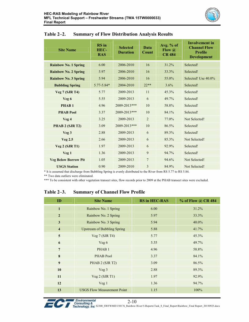
Upon review of the flow distribution analysis results summarized in Table 2-2, it was
concluded that only selected flow measurement sites were used in developing the channel
flow profile due to the following considerations:
First of all, the SWFWMD flow measurement sites near various vegetation
transect locations have a higher priority over the USGS sites at the springs.
Veg 4 and USGS Station – not selected due to limited amount of flow records.
Veg 2.5 and Veg below Borrow Pit (BBP) – not selected in order to maintain an
incremental flow profile along the river reach.
Rainbow No. 3 Spring – percentage of flow at CR 484 Bridge was reduced from
55% to 40% using professional judgment, which is lower than the percentage
value of 41.7% estimated at upstream of Bubbling Spring (45.3% at Veg 7 minus
3.6% from Bubbling Spring), as shown in Table 2-3. The flow percentage
difference between Rainbow No. 3 Spring at RS 5.94 and upstream of Bubbling
Spring at RS 5.88 is calculated at 1.7%, which seems a reasonable estimate to
account for any incidental groundwater inflows between these two river stations.
Per Water-Year summary for USGS Gage 02313100, the flow measurement for this gage
was conducted at 0.25 mile upstream of CR 484 Bridge or RS 1.15 in the HEC-RAS
model set up. It is assumed that no additional groundwater or surface water discharges to
the river reach downstream of RS 1.15; and therefore, 100% of flow at CR 484 Bridge
was defined at this location.
In summary, a total of 13 cross-sections or river stations have been assigned with a flow
relationship between the cross-section and USGS 02313100 Rainbow River at
Dunnellon, Florida, as listed in Table 2-3. Note that at RS 5.88 the percentage value of
41.7% was estimated by subtracting the discharge from Bubbling Spring (3.6%, see
Table 2-2) from the value of 45.3% at Veg 7 (SJR T4).
A linear interpolation approach was used to generate the flow values at each cross-section
depending on its distances to the 13 cross-sections or river stations listed in Table 2-3.

HEC-RAS Modeling of Rainbow River MFL Technical Support – Freshwater Streams (TWA 15TW0000033) Final Report
2-9 P:\S2300_SWFWMD\150176_Rainbow River\5-Reports\Task_8_Final_Report\Rainbow_Final Report_20150925.docx
Figure 2-5. Locations of USGS/SWFWMD Flow/Stage Measurement
in Rainbow River
HEC-RAS Modeling of Rainbow River MFL Technical Support – Freshwater Streams (TWA 15TW0000033) Final Report
2-10 P:\S2300_SWFWMD\150176_Rainbow River\5-Reports\Task_8_Final_Report\Rainbow_Final Report_20150925.docx
Table 2–2. Summary of Flow Distribution Analysis Results
Site Name RS in HEC-RAS
Selected Duration
Data Count
Avg. % of Flow @ CR 484
Involvement in Channel Flow
Profile Development
Rainbow No. 1 Spring 6.00 2006-2010 16 31.2% Selected!
Rainbow No. 2 Spring 5.97 2006-2010 16 33.3% Selected!
Rainbow No. 3 Spring 5.94 2006-2010 16 55.0% Selected! Use 40.0%
Bubbling Spring 5.77-5.84* 2004-2010 22** 3.6% Selected!
Veg 7 (SJR T4) 5.77 2009-2013 11 45.3% Selected!
Veg 6 5.55 2009-2013 6 49.7% Selected!
PHAB 1 4.96 2009-2013*** 10 58.8% Selected!
PHAB Pool 3.37 2009-2013*** 10 84.1% Selected!
Veg 4 3.25 2009-2013 2 77.0% Not Selected!
PHAB 2 (SJR T2) 3.09 2009-2013*** 10 86.5% Selected!
Veg 3 2.88 2009-2013 6 89.3% Selected!
Veg 2.5 2.66 2009-2013 6 85.3% Not Selected!
Veg 2 (SJR T1) 1.97 2009-2013 6 92.9% Selected!
Veg 1 1.36 2009-2013 9 94.7% Selected!
Veg Below Borrow Pit 1.05 2009-2013 7 94.6% Not Selected!
USGS Station 0.90 2009-2010 3 84.9% Not Selected! * It is assumed that discharge from Bubbling Spring is evenly distributed to the River from RS 5.77 to RS 5.84. ** Two data outliers were eliminated. *** To be consistent with other vegetation transect sites, flow records prior to 2009 at the PHAB transect sites were excluded.
Table 2–3. Summary of Channel Flow Profile
ID Site Name RS in HEC-RAS % of Flow @ CR 484
1 Rainbow No. 1 Spring 6.00 31.2%
2 Rainbow No. 2 Spring 5.97 33.3%
3 Rainbow No. 3 Spring 5.94 40.0%
4 Upstream of Bubbling Spring 5.88 41.7%
5 Veg 7 (SJR T4) 5.77 45.3%
6 Veg 6 5.55 49.7%
7 PHAB 1 4.96 58.8%
8 PHAB Pool 3.37 84.1%
9 PHAB 2 (SJR T2) 3.09 86.5%
10 Veg 3 2.88 89.3%
11 Veg 2 (SJR T1) 1.97 92.9%
12 Veg 1 1.36 94.7%
13 USGS Flow Measurement Point 1.15 100%

HEC-RAS Modeling of Rainbow River MFL Technical Support – Freshwater Streams (TWA 15TW0000033) Final Report
2-11 P:\S2300_SWFWMD\150176_Rainbow River\5-Reports\Task_8_Final_Report\Rainbow_Final Report_20150925.docx
2.3.2 DOWNSTREAM BOUNDARY CONDITIONS
Generally, the downstream boundary will be selected at a USGS gage station where a
USGS stage-flow rating curve is available. However, a defined stage-flow rating curve is
not available at the selected downstream boundary at USGS 02313100 Rainbow River at
Dunnellon, Florida (CR 484 Bridge), mostly due to the severe backwater effects from
Withlacoochee River through a short river reach, approximately 0.9 mile, between the
gage at CR 484 Bridge and the river confluence.
A simple linear regression method, with one independent variable X – Flow at USGS
Gage 02313100, was first employed to develop a stage-flow rating curve at USGS Gage
02313100. The flow/stage records at this USGS gage, in a period of 2005 through 2013,
were utilized in the regression analysis. The resultant regression curve is plotted in Figure
2-6, with a coefficient of multiple determination (R2) value of 0.5258.
Figure 2-6. Simple Linear Regression Curve at USGS 02313100
Model a*x 3̂+b*x 2̂+c*x+d
Y -
Sta
ge @
CR
484 B
ridge (
ft-N
AV
D)
X - Flow @ CR 484 Bridge (CFS)
25.5
26.0
26.5
27.0
27.5
28.0
28.5
29.0
350.0 400.0 450.0 500.0 550.0 600.0 650.0 700.0 750.0 800.0
USGS Gage Dataa*x^3+b*x^2+c*x+d
a = 1.486166601E-007
b = -0.0002657810491
c = 0.1592523627
d = -4.678130539
R2 = 0.5258

HEC-RAS Modeling of Rainbow River MFL Technical Support – Freshwater Streams (TWA 15TW0000033) Final Report
2-12 P:\S2300_SWFWMD\150176_Rainbow River\5-Reports\Task_8_Final_Report\Rainbow_Final Report_20150925.docx
Upon review of the historic stage/flow records at the two USGS long-term gages, USGS
02313100 Rainbow River at Dunnellon, Florida and USGS 02313200 Withlacoochee
River at Dunnellon, Florida (Figure 2-1), it is deemed feasible to improve the rating curve
described above by implementing multiple regression method and the historic stage/flow
data at these two USGS gages.
In the multiple regression analysis, two independent variables were involved: X1 - Flow
at USGS 02313100 at CR 484 bridge; and X2 - Stage at USGS 02313200 Withlacoochee
River at Dunnellon, Florida (US 41 bridge), and the dependent variable is Y - Stage of
USGS 02313100 at CR 484 Bridge. The flow/stage records in a period of 3/112005
through 9/30/2013 were utilized in the multiple regression analysis. The resultant
multiple regression curve is plotted in Figure 2-7, with a significantly improved R2 value
of 0.9860.
Figure 2-7. Multiple Regression Curve at USGS 02313100
Model a+b*x1+c*x1 2̂+d*x1 3̂+e*x2
Y -
Sta
ge @
CR
484 B
ridge (
ft-N
AV
D)
Y -
Sta
ge @
CR
484 B
ridge (
ft-N
AV
D)
X2 - Stage @ Withlacoochee River (ft-NAVD) X1 - Flow @ CR 484 Bridge (CFS)
25.526.0
26.527.0
27.528.0
750.0700.0650.0600.0550.0500.0450.0400.0350.0
25.5
26.0
26.5
27.0
27.5
28.0
28.5
29.0
25.5
26.0
26.5
27.0
27.5
28.0
28.5
29.0
USGS Gage Dataa+b*x1+c*x1^2+d*x1^3+e*x2
a = -1.903647847
b = 0.009929658
c = -2.021798675E-05
d = 1.361798027E-08
e = 1.016261988
R2 = 0.9860

HEC-RAS Modeling of Rainbow River MFL Technical Support – Freshwater Streams (TWA 15TW0000033) Final Report
2-13 P:\S2300_SWFWMD\150176_Rainbow River\5-Reports\Task_8_Final_Report\Rainbow_Final Report_20150925.docx
To verify whether these two “independent” variables used in the multiple regression
analysis are correlated with each other or not, a linear regression analysis was performed
based on the stage data at USGS 02313200 and flow data at USGS 02313100. The
resultant linear regression curve is plotted in Figure 2-8, with a R2 value of 0.1159, which
suggests there is a very weak correlation between the stage in Withlacoochee River and
the flow in Rainbow River. Therefore, the multiple regression analysis with these two
“independent” variables seems appropriate in general.
Figure 2-8. Stage at USGS 02313200 vs. Flow at USGS 02313100
In summary, at the downstream boundary of USGS Gage 02313100, the stage-flow rating
curve has been significantly improved by using multiple regression method (Figure 2-7).
However, for a given flow scenario to be simulated in HEC-RAS, two independent
variables - flow in Rainbow River and stage in Withlacoochee River, have to be defined
prior to estimating an reasonable boundary condition (stage) at CR 484 Bridge.
y = 0.0015x + 26.108 R² = 0.1159
22
23
24
25
26
27
28
29
30
31
32
300 400 500 600 700 800 900 1000 1100
Sta
ge a
t U
SG
S 0
2313200 (
US
41 B
rid
ge)
(ft-
NA
VD
)
Flow at USGS 02313100 (CR 484 Bridge) (cfs)

HEC-RAS Modeling of Rainbow River MFL Technical Support – Freshwater Streams (TWA 15TW0000033) Final Report
2-14 P:\S2300_SWFWMD\150176_Rainbow River\5-Reports\Task_8_Final_Report\Rainbow_Final Report_20150925.docx
2.3.3 STEADY-STATE MODEL SIMULATION
To identify any potential errors or omissions in the geometric data of the preliminary
HEC-RAS model of Rainbow River, a steady-state flow scenario was developed and
simulated. The steady-state flow scenario assumed a 50 percentile (P50) flow condition
in both Rainbow River and Withlacoochee River.
The channel flow profile and downstream boundary condition for the P50 flow scenario
were first formulated using the methodology discussed in Sections 2.3.1 and 2.3.2, and
stored in an Excel working spreadsheet prior to being imported into the HEC-RAS
model. Computation message of the steady-state flow analysis was reviewed to fix errors
or warnings in the river geometric data and flow profile data, if any.
The stage profile plot for this steady-state flow scenario is presented in Figure 2-9. The
stage profile plot could be used to check the overall water elevation profile for a given
flow scenario, or be zoomed in to identify the type of flow profile, e.g., M1 profile.
Figure 2-9. Stage Profile Plot of P50 Steady-State Flow Scenario in Rainbow
River
0 5000 10000 15000 20000 25000 3000010
15
20
25
30
35
Rainbow_V1 Plan: Rainbow_V1_50% 4/23/2015
Main Channel Distance (ft)
Ele
vation
(ft)
Legend
WS 50%
Ground
1.0
01
.09
1.1
81
.28
1.3
71
.46
1.5
61
.65
1.7
41
.84
1.9
32
.02
2.1
22
.21
2.3
02
.40
2.4
92
.58
2.6
82
.77
2.8
62
.96
3.0
53
.14
3.2
33
.33
3.4
23
.51
3.6
13
.70
3.7
93
.89
3.9
84
.07
4.1
74
.26
4.3
54
.45
4.5
44
.63
4.7
34
.82
4.9
15
.01
5.1
05
.19
5.2
95
.38
5.4
75
.57
5.6
65
.75
5.8
45
.94
Rainbow Main

HEC-RAS Modeling of Rainbow River MFL Technical Support – Freshwater Streams (TWA 15TW0000033) Final Report
3-1 P:\S2300_SWFWMD\150176_Rainbow River\5-Reports\Task_8_Final_Report\Rainbow_Final Report_20150925.docx
3. HEC-RAS MODEL CALIBRATION
3.1 GAGE DATA ANALYSIS
Long-term daily flow and stage data at USGS gages is usually required to develop the
dynamic flow and stage hydrographs used at boundary conditions for a dynamic HEC-
RAS model analysis. Two long-term USGS gages in the Rainbow and Withlacoochee
Rivers, as listed below and presented in Figure 3-1 and Table 3-1, are employed in
developing the dynamic flow and stage hydrographs to be used in the dynamic HEC-RAS
model.
USGS 02313100 Rainbow River at Dunnellon, Florida at CR 484 Bridge provides
long-term daily average flow and stage data at the downstream boundary of the
HEC-RAS model.
USGS 02313200 Withlacoochee River at Dunnellon, Florida at U.S. Highway 41
Bridge provides long-term daily average stage data that was used to estimate the
missing stage data at USGS 02313100 in the Rainbow River (River).
Short-term stage data collected at various gage stations and vegetation transect sites
facilitates comparison with the model predicted water level elevations at the same
locations, for model calibration or verification purposes. Four agencies, including USGS,
FDEP, SWFWMD, and SJRWMD, have conducted miscellaneous stage measurements at
a total of 14 river stations or sites along the river segment as shown in Figure 3-1 and
listed in Table 3-1.

HEC-RAS Modeling of Rainbow River MFL Technical Support – Freshwater Streams (TWA 15TW0000033) Final Report
3-2 P:\S2300_SWFWMD\150176_Rainbow River\5-Reports\Task_8_Final_Report\Rainbow_Final Report_20150925.docx
Figure 3-1. Stream Gages in Rainbow and Withlacoochee Rivers

HEC-RAS Modeling of Rainbow River MFL Technical Support – Freshwater Streams (TWA 15TW0000033) Final Report
3-3 P:\S2300_SWFWMD\150176_Rainbow River\5-Reports\Task_8_Final_Report\Rainbow_Final Report_20150925.docx
Table 3–1. Summary of Stage Datasets in Rainbow and Withlacoochee Rivers
Station/Site Name
Station ID Agency
RS in HEC-RAS
Start Date End Date* Stage Data**
Count
Rainbow River at Spring Head*** FDEP 6.00 10/8/2005 1/25/2013 582
Rainbow River at Spring Head*** USGS 6.00 1/14/1965 1/31/2012 224
Veg 7**** SWFWMD 5.77 7/1/2009 3/12/2015 34
Veg 7 SWFWMD 5.77 5/22/2014 9/2/2014 2,473 (hourly)
SJR T4 SJRWMD 5.77 9/1/2009 9/26/2011 712 (daily)
Veg 6**** SWFWMD 5.55 7/1/2009 3/12/2015 21
PHAB 1**** SWFWMD 4.96 8/17/2005 3/12/2015 47
SJR T3 SJRWMD 4.31 9/1/2009 9/27/2011 757 (daily)
PHAB Pool**** SWFWMD 3.37 8/30/2005 3/12/2015 38
Rainbow River near Dunnellon 02313098 USGS 3.33 11/15/2013 3/17/2015 47,098 (15-min)
483 (daily)
Veg 4**** SWFWMD 3.25 7/1/2009 7/29/2009 3
PHAB 2**** SWFWMD 3.09 8/11/2005 3/12/2015 46
PHAB 2 SWFWMD 3.09 3/10/2014 2/9/2015 8,065 (hourly)
SJR T2 SJRWMD 3.09 9/1/2009 9/26/2011 687 (daily)
Veg 3**** SWFWMD 2.88 7/14/2009 3/12/2015 27
Veg 2.5**** SWFWMD 2.66 7/1/2009 3/12/2015 31
Veg 2**** SWFWMD 1.97 7/1/2009 3/12/2015 31
SJR T1 SJRWMD 1.97 9/2/2009 9/26/2011 706 (daily)
Veg 1**** SWFWMD 1.36 7/1/2009 3/12/2015 40
Veg 1 SWFWMD 1.36 9/24/2009 2/9/2015 3,311 (hourly)
Veg Below Borrow Pit (BBP) **** SWFWMD 1.05 7/1/2009 3/12/2015 31
Rainbow River at Dunnellon 02313100 USGS 0.90 3/11/2005 3/17/2015 3,245 (daily)
Withlacoochee River at Dunnellon 02313200 USGS - 2/6/1963 3/17/2015 18,896 (daily)
Notes: RS – River station is measured in river miles from the river confluence at the Withlacoochee River. * End date of the USGS stage data was selected at the end of the simulation span (3/11/2005 -3/17/2015) of the dynamic
HEC-RAS model. ** 15-min, hourly, and daily stage data was derived from the real-time data loggers installed by USGS, SWFWMD, and
SJRWMD at various gage locations. *** Stage data at the spring head was either read from staff gage by FDEP staff (Mr. Jeff Sowards) or measured by USGS staff. **** Stage data was read from staff gage or surveyed at the same day when flow measurement was conducted at these
vegetation transects.
HEC-RAS Modeling of Rainbow River MFL Technical Support – Freshwater Streams (TWA 15TW0000033) Final Report
3-4 P:\S2300_SWFWMD\150176_Rainbow River\5-Reports\Task_8_Final_Report\Rainbow_Final Report_20150925.docx
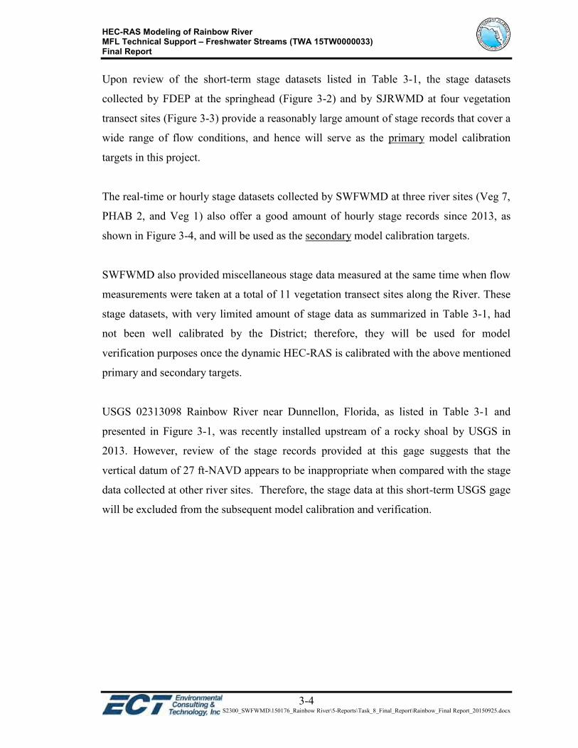
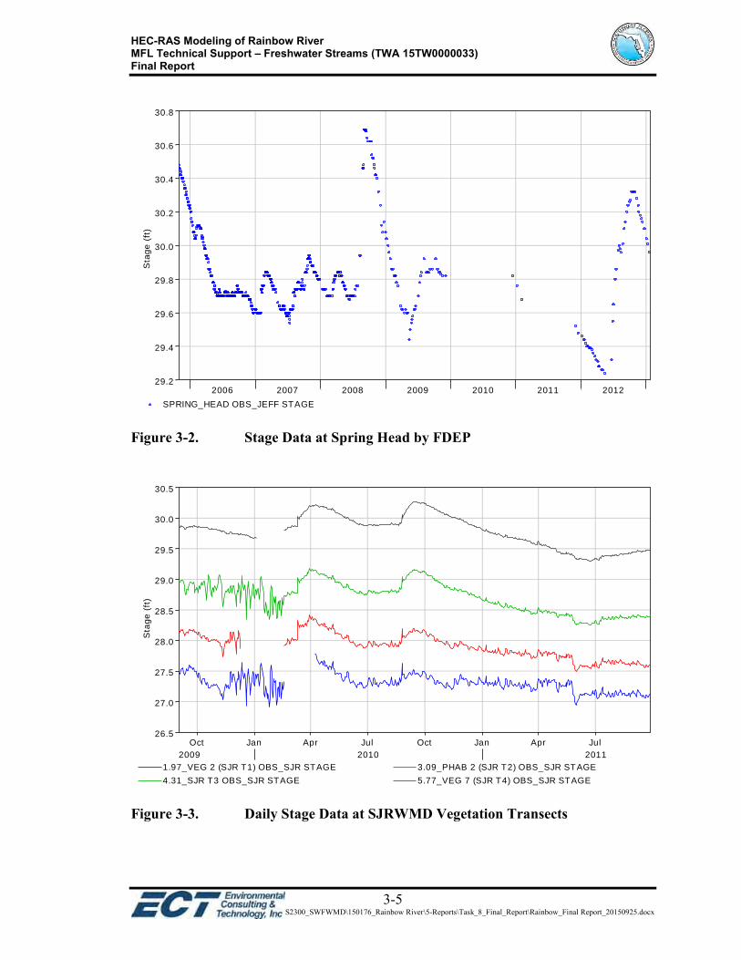
Upon review of the short-term stage datasets listed in Table 3-1, the stage datasets
collected by FDEP at the springhead (Figure 3-2) and by SJRWMD at four vegetation
transect sites (Figure 3-3) provide a reasonably large amount of stage records that cover a
wide range of flow conditions, and hence will serve as the primary model calibration
targets in this project.
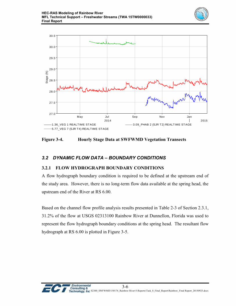
The real-time or hourly stage datasets collected by SWFWMD at three river sites (Veg 7,
PHAB 2, and Veg 1) also offer a good amount of hourly stage records since 2013, as
shown in Figure 3-4, and will be used as the secondary model calibration targets.
SWFWMD also provided miscellaneous stage data measured at the same time when flow
measurements were taken at a total of 11 vegetation transect sites along the River. These
stage datasets, with very limited amount of stage data as summarized in Table 3-1, had
not been well calibrated by the District; therefore, they will be used for model
verification purposes once the dynamic HEC-RAS is calibrated with the above mentioned
primary and secondary targets.
USGS 02313098 Rainbow River near Dunnellon, Florida, as listed in Table 3-1 and
presented in Figure 3-1, was recently installed upstream of a rocky shoal by USGS in
2013. However, review of the stage records provided at this gage suggests that the
vertical datum of 27 ft-NAVD appears to be inappropriate when compared with the stage
data collected at other river sites. Therefore, the stage data at this short-term USGS gage
will be excluded from the subsequent model calibration and verification.
HEC-RAS Modeling of Rainbow River MFL Technical Support – Freshwater Streams (TWA 15TW0000033) Final Report
3-5 P:\S2300_SWFWMD\150176_Rainbow River\5-Reports\Task_8_Final_Report\Rainbow_Final Report_20150925.docx
Figure 3-2. Stage Data at Spring Head by FDEP
Figure 3-3. Daily Stage Data at SJRWMD Vegetation Transects
2006 2007 2008 2009 2010 2011 2012
Sta
ge
(ft
)
29.2
29.4
29.6
29.8
30.0
30.2
30.4
30.6
30.8
SPRING_HEAD OBS_JEFF STAGE
Oct Jan Apr Jul Oct Jan Apr Jul
2009 2010 2011
Sta
ge
(ft
)
26.5
27.0
27.5
28.0
28.5
29.0
29.5
30.0
30.5
1.97_VEG 2 (SJR T1) OBS_SJR STAGE 3.09_PHAB 2 (SJR T2) OBS_SJR STAGE
4.31_SJR T3 OBS_SJR STAGE 5.77_VEG 7 (SJR T4) OBS_SJR STAGE
HEC-RAS Modeling of Rainbow River MFL Technical Support – Freshwater Streams (TWA 15TW0000033) Final Report
3-6 P:\S2300_SWFWMD\150176_Rainbow River\5-Reports\Task_8_Final_Report\Rainbow_Final Report_20150925.docx
Figure 3-4. Hourly Stage Data at SWFWMD Vegetation Transects
3.2 DYNAMIC FLOW DATA – BOUNDARY CONDITIONS
3.2.1 FLOW HYDROGRAPH BOUNDARY CONDITIONS
A flow hydrograph boundary condition is required to be defined at the upstream end of
the study area. However, there is no long-term flow data available at the spring head, the
upstream end of the River at RS 6.00.
Based on the channel flow profile analysis results presented in Table 2-3 of Section 2.3.1,
31.2% of the flow at USGS 02313100 Rainbow River at Dunnellon, Florida was used to
represent the flow hydrograph boundary conditions at the spring head. The resultant flow
hydrograph at RS 6.00 is plotted in Figure 3-5.
May Jul Sep Nov Jan
2014 2015
Sta
ge
(ft
)
27.0
27.5
28.0
28.5
29.0
29.5
30.0
30.5
1.36_VEG 1 REALTIME STAGE 3.09_PHAB 2 (SJR T2) REALTIME STAGE
5.77_VEG 7 (SJR T4) REALTIME STAGE

HEC-RAS Modeling of Rainbow River MFL Technical Support – Freshwater Streams (TWA 15TW0000033) Final Report
3-7 P:\S2300_SWFWMD\150176_Rainbow River\5-Reports\Task_8_Final_Report\Rainbow_Final Report_20150925.docx
Figure 3-5. Flow Hydrograph at RS 6.00 (Spring Head)
3.2.2 STAGE HYDROGRAPH BOUNDARY CONDITIONS
A stage hydrograph boundary condition is defined at RS 0.89, the downstream end of the
River located downstream of CR 484 Bridge. The cross-section at RS 0.89 was
intentionally added to the river geometric data, as HEC-RAS requires at least two cross-
sections downstream of a structure to run dynamic flow analysis. The stage records of
USGS 02313100 Rainbow River at Dunnellon, Florida at CR 484 Bridge (RS 0.90) are
used to define the stage hydrograph boundary conditions at RS 0.89, by assuming there is
no noticeable head loss between the gage location and downstream boundary node.
Stage records at this gage are missing for entire Water Year (WY) of 2014. Data filling
was performed by using the multiple regression curve previously developed in this
project (Section 2.3.2). The flow data provided at this gage and the stage data at USGS
02313200 Withlacoochee River at Dunnellon, Florida are the two independent variables
used in the multiple regression analysis.
2005 2006 2007 2008 2009 2010 2011 2012 2013 2014
Flo
w (
cfs
)
120
140
160
180
200
220
240
RS 6.00 (SPRING HEAD) 31.2% OF FLOW AT USGS 02313100

HEC-RAS Modeling of Rainbow River MFL Technical Support – Freshwater Streams (TWA 15TW0000033) Final Report
3-8 P:\S2300_SWFWMD\150176_Rainbow River\5-Reports\Task_8_Final_Report\Rainbow_Final Report_20150925.docx
The stage hydrograph at RS 0.89, consisting of the stage records obtained from USGS
and the values estimated using the multiple regression analysis for WY 2014, is plotted in
Figure 3-6.
Figure 3-6. Stage Hydrograph at RS 0.89 (CR 484 Bridge)
3.2.3 LATERAL INFLOW HYDROGRAPH BOUNDARY CONDITIONS
The lateral inflow hydrograph is used as an internal boundary condition in HEC-RAS to
represent inflow, e.g., surface water inflow from a tributary or groundwater inflow from a
spring, at a specified point or cross-section along the river reach. In the dynamic HEC-
RAS model of Rainbow River, two lateral inflow hydrograph boundary conditions were
defined at RS 5.97 and RS 5.94 to represent the groundwater inflow from Rainbow No. 2
Spring and Rainbow No. 3 Spring, respectively, as listed in Table 3-2.
The uniform lateral inflow hydrograph is used as an internal boundary condition in HEC-
RAS to represent uniformly distributed inflow along the river reach between two
specified cross-section locations. The uniform lateral inflow hydrograph is very useful
when the inflow could not be assigned to a specified point along the river reach, e.g.,
2005 2006 2007 2008 2009 2010 2011 2012 2013 2014
Sta
ge
(ft
)
25.5
26.0
26.5
27.0
27.5
28.0
28.5
29.0
RS 0.89 (USGS 02313100) OBS_SYN STAGE

HEC-RAS Modeling of Rainbow River MFL Technical Support – Freshwater Streams (TWA 15TW0000033) Final Report
3-9 P:\S2300_SWFWMD\150176_Rainbow River\5-Reports\Task_8_Final_Report\Rainbow_Final Report_20150925.docx
multiple small springs or surface water runoff along a river reach. A total of 10 uniform
lateral inflow hydrograph boundary conditions were defined in the dynamic HEC-RAS
model, between RS 5.91 and RS 1.15 to represent the groundwater and surface water
inflows along the River, as listed in Table 3-2.
The percentage values of listed in Table 3-2 were derived from the channel flow profile
analysis results presented in Table 2-3 of Section 2.3.1. The total flow percentage values
for the lateral/uniform lateral inflow hydrographs is 68.8% of flow at CR 484, as plotted
in Figure 3-7. The remaining 31.2% of flow at CR 484 has been assigned to the spring
head at RS 6.00, modeled as a flow hydrograph boundary condition in Section 3.2.1.
Note that it is not practical to develop time-variant percentage values at each river site in
long-term dynamic flow analysis, mostly due to the very limited flow measurement data
in the study area (Table 2-2).
Table 3–2 Summary of Lateral/Uniform Lateral Inflow Hydrograph Boundary Conditions
ID RS in HEC-RAS
% of Flow @ CR 484
Boundary Condition Type Comments
1 5.97 2.10% Lateral Inflow Rainbow No. 2 Spring and others
2 5.94 6.70% Lateral Inflow Rainbow No. 3 Spring and others
3 5.91 - 5.88 1.70% Uniform Lateral Inflow Waterfall Spring and others
4 5.88 - 5.77 3.60% Uniform Lateral Inflow Bubbling Spring
5 5.77 - 5.55 4.40% Uniform Lateral Inflow Between Veg 7 (SJR T4) and Veg 6
6 5.55 - 4.96 9.10% Uniform Lateral Inflow Between Veg 6 and PHAB 1
7 4.96 - 3.37 25.30% Uniform Lateral Inflow Between PHAB 1 and PHAB Pool
8 3.37 - 3.09 2.40% Uniform Lateral Inflow Between PHAB Pool and PHAB 2 (SJR T2)
9 3.09 - 2.88 2.80% Uniform Lateral Inflow Between PHAB 2 (SJR T2) and Veg 3
10 2.88 - 1.97 3.60% Uniform Lateral Inflow Between Veg 3 and Veg 2 (SJR T1)
11 1.97 - 1.36 1.80% Uniform Lateral Inflow Between Veg 2 (SJR T1) and Veg 1
12 1.36 - 1.15 5.30% Uniform Lateral Inflow USGS Flow Measurement Point
Total: 68.8 %

HEC-RAS Modeling of Rainbow River MFL Technical Support – Freshwater Streams (TWA 15TW0000033) Final Report
3-10 P:\S2300_SWFWMD\150176_Rainbow River\5-Reports\Task_8_Final_Report\Rainbow_Final Report_20150925.docx
Figure 3-7. Accumulated Lateral/Uniform Lateral Inflow Hydrographs from
RS 5.97 to 1.15 (Downstream of Spring Head)
3.3 DYNAMIC HEC-RAS MODEL SIMULATION AND CALIBRATION
3.3.1 MODEL SIMULATION
A total of 10 years from 3/11/2005 to 3/17/2015 are selected as a simulation span for
unsteady flow analysis of the Rainbow River. As discussed in the previous section, all
required boundary conditions have been developed and stored in several DSS database
files to be used for the unsteady flow analysis in HEC-RAS.
The boundary conditions and initial conditions are defined in the “Unsteady Flow
Analysis Editor” in HEC-RAS.
3.3.2 MODEL STABILIZATION
During low flow conditions, the unsteady flow simulation is expected to fail at certain
hydraulic critical points of the River, where subcritical flow changes to supercritical flow
within a very short distance (i.e., rocky shoal near RS 3.10). To improve model stability
of the dynamic HEC-RAS model at the hydraulic critical points, Manning’s n values
2005 2006 2007 2008 2009 2010 2011 2012 2013 2014
Flo
w (
cfs
)
250
300
350
400
450
500
550
RS 5.97 - 1.15 (DOWNSTREAM OF SPRING HEAD) 68.8% OF FLOW AT USGS 02313100
HEC-RAS Modeling of Rainbow River MFL Technical Support – Freshwater Streams (TWA 15TW0000033) Final Report
3-11 P:\S2300_SWFWMD\150176_Rainbow River\5-Reports\Task_8_Final_Report\Rainbow_Final Report_20150925.docx
were adjusted in order to increase critical water depth and reduce Froude number.
Adding interpolated cross-sections and/or reducing computation interval were also
considered, if the instability still exists. Upon a few iterations of model coefficient
adjustments, the dynamic HEC-RAS model was stabilized to be able to simulate all flow
conditions experienced within the 10-year simulation span.
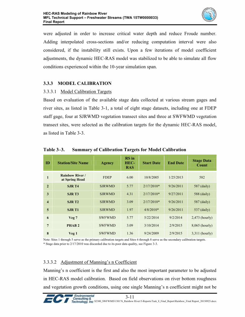
3.3.3 MODEL CALIBRATION
3.3.3.1 Model Calibration Targets
Based on evaluation of the available stage data collected at various stream gages and
river sites, as listed in Table 3-1, a total of eight stage datasets, including one at FDEP
staff gage, four at SJRWMD vegetation transect sites and three at SWFWMD vegetation
transect sites, were selected as the calibration targets for the dynamic HEC-RAS model,
as listed in Table 3-3.
Table 3–3. Summary of Calibration Targets for Model Calibration
ID Station/Site Name Agency RS in HEC-RAS
Start Date End Date Stage Data Count
1 Rainbow River / at Spring Head FDEP 6.00 10/8/2005 1/25/2013 582
2 SJR T4 SJRWMD 5.77 2/17/2010* 9/26/2011 587 (daily)
3 SJR T3 SJRWMD 4.31 2/17/2010* 9/27/2011 588 (daily)
4 SJR T2 SJRWMD 3.09 2/17/2010* 9/26/2011 587 (daily)
5 SJR T1 SJRWMD 1.97 4/8/2010* 9/26/2011 537 (daily)
6 Veg 7 SWFWMD 5.77 5/22/2014 9/2/2014 2,473 (hourly)
7 PHAB 2 SWFWMD 3.09 3/10/2014 2/9/2015 8,065 (hourly)
8 Veg 1 SWFWMD 1.36 9/24/2009 2/9/2015 3,311 (hourly)
Note: Sites 1 through 5 serve as the primary calibration targets and Sites 6 through 8 serve as the secondary calibration targets. * Stage data prior to 2/17/2010 was discarded due to its poor data quality, see Figure 3-3.
3.3.3.2 Adjustment of Manning’s n Coefficient
Manning’s n coefficient is the first and also the most important parameter to be adjusted
in HEC-RAS model calibration. Based on field observations on river bottom roughness
and vegetation growth conditions, using one single Manning’s n coefficient might not be

HEC-RAS Modeling of Rainbow River MFL Technical Support – Freshwater Streams (TWA 15TW0000033) Final Report
3-12 P:\S2300_SWFWMD\150176_Rainbow River\5-Reports\Task_8_Final_Report\Rainbow_Final Report_20150925.docx
adequate to represent the real roughness of the river under different flow conditions.
Roughness generally decreased with increases flow and depth. This is especially true for
the river segment upstream of the rocky shoal near RS 3.10, where the aquatic plant
overgrowth could dramatically increase river bottom roughness with reduced flow and
depth.
Therefore, to improve the model calibration results, roughness coefficients were
automatically adjusted in HEC-RAS with changes in flow, using a set of flow roughness
factors at each cross-section. Table 3-4 provides a set of flow roughness factors in
corresponding to the flow at CR 484 Bridge (RS 0.89). Between the flows listed in this
table, HEC-RAS will use linear interpolation to obtain a roughness factor (Brunner,
2010b). The flow roughness factors in the cross-sections from RS 3.11 to RS 6.00 could
be developed by varying flow rates based on the flow profile analysis results listed in
Table 2-3 of Section 2.3.1. Note that no flow roughness factors were used in the cross-
sections downstream of the rocky shoal (RS 3.11) due to less vegetation overgrowth
observed in this river segment.
In summary, flow roughness factors provide the modeler a more effective and flexible
tool to meet the calibration targets under different flow conditions.
Table 3–4. Summary of Flow Roughness Factors in Cross-Sections (RS 3.11 - 6.00)
ID Flow at CR 484 (CFS) Roughness Factor
1 350 1.25
2 400 1.2
3 450 1.1
4 500 1.0
5 550 1.0
6 600 1.0
7 800 1.0
8 1000 1.0
HEC-RAS Modeling of Rainbow River MFL Technical Support – Freshwater Streams (TWA 15TW0000033) Final Report
3-13 P:\S2300_SWFWMD\150176_Rainbow River\5-Reports\Task_8_Final_Report\Rainbow_Final Report_20150925.docx
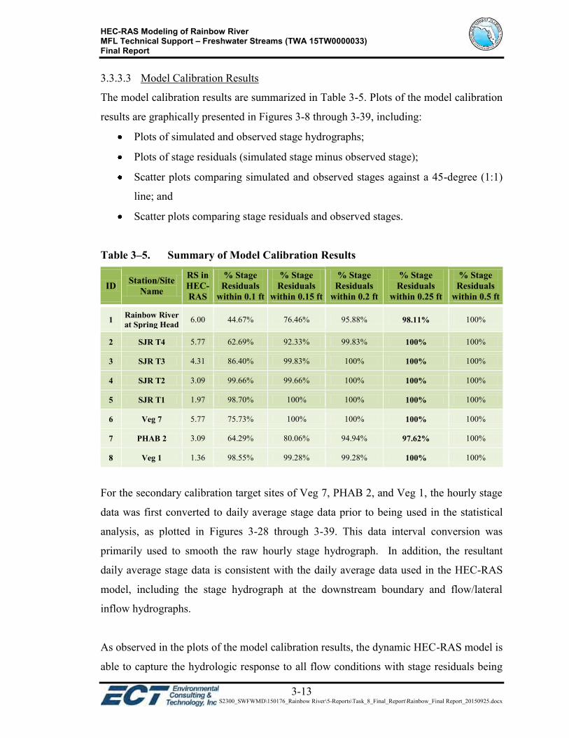
3.3.3.3 Model Calibration Results
The model calibration results are summarized in Table 3-5. Plots of the model calibration
results are graphically presented in Figures 3-8 through 3-39, including:
Plots of simulated and observed stage hydrographs;
Plots of stage residuals (simulated stage minus observed stage);
Scatter plots comparing simulated and observed stages against a 45-degree (1:1)
line; and
Scatter plots comparing stage residuals and observed stages.
Table 3–5. Summary of Model Calibration Results
ID Station/Site Name
RS in HEC-RAS
% Stage Residuals
within 0.1 ft
% Stage Residuals
within 0.15 ft
% Stage Residuals
within 0.2 ft
% Stage Residuals
within 0.25 ft
% Stage Residuals
within 0.5 ft
1 Rainbow River at Spring Head 6.00 44.67% 76.46% 95.88% 98.11% 100%
2 SJR T4 5.77 62.69% 92.33% 99.83% 100% 100%
3 SJR T3 4.31 86.40% 99.83% 100% 100% 100%
4 SJR T2 3.09 99.66% 99.66% 100% 100% 100%
5 SJR T1 1.97 98.70% 100% 100% 100% 100%
6 Veg 7 5.77 75.73% 100% 100% 100% 100%
7 PHAB 2 3.09 64.29% 80.06% 94.94% 97.62% 100%
8 Veg 1 1.36 98.55% 99.28% 99.28% 100% 100%
For the secondary calibration target sites of Veg 7, PHAB 2, and Veg 1, the hourly stage
data was first converted to daily average stage data prior to being used in the statistical
analysis, as plotted in Figures 3-28 through 3-39. This data interval conversion was
primarily used to smooth the raw hourly stage hydrograph. In addition, the resultant
daily average stage data is consistent with the daily average data used in the HEC-RAS
model, including the stage hydrograph at the downstream boundary and flow/lateral
inflow hydrographs.
As observed in the plots of the model calibration results, the dynamic HEC-RAS model is
able to capture the hydrologic response to all flow conditions with stage residuals being
HEC-RAS Modeling of Rainbow River MFL Technical Support – Freshwater Streams (TWA 15TW0000033) Final Report
3-14 P:\S2300_SWFWMD\150176_Rainbow River\5-Reports\Task_8_Final_Report\Rainbow_Final Report_20150925.docx
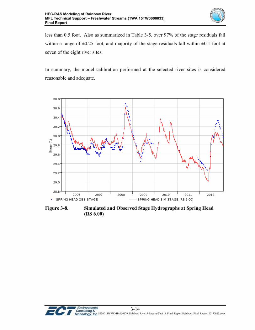
less than 0.5 foot. Also as summarized in Table 3-5, over 97% of the stage residuals fall
within a range of ±0.25 foot, and majority of the stage residuals fall within ±0.1 foot at
seven of the eight river sites.
In summary, the model calibration performed at the selected river sites is considered
reasonable and adequate.
Figure 3-8. Simulated and Observed Stage Hydrographs at Spring Head
(RS 6.00)
2006 2007 2008 2009 2010 2011 2012
Sta
ge
(ft
)
28.8
29.0
29.2
29.4
29.6
29.8
30.0
30.2
30.4
30.6
30.8
SPRING HEAD OBS STAGE SPRING HEAD SIM STAGE (RS 6.00)

HEC-RAS Modeling of Rainbow River MFL Technical Support – Freshwater Streams (TWA 15TW0000033) Final Report
3-15 P:\S2300_SWFWMD\150176_Rainbow River\5-Reports\Task_8_Final_Report\Rainbow_Final Report_20150925.docx
Figure 3-9. Stage Residuals at Spring Head (RS 6.00)
Figure 3-10. Scatter Plot Comparing Simulated and Observed Stages
at Spring Head (RS 6.00)
2006 2007 2008 2009 2010 2011 2012
Sta
ge
Dif
fere
nc
e (
Sim
-Ob
s)
(ft)
-0.4
-0.3
-0.2
-0.1
0.0
0.1
0.2
0.3
0.4
STAGE RESIDUAL AT SPRING HEAD (RS 6.00)
Observed Stage (ft)
29 29.2 29.4 29.6 29.8 30 30.2 30.4 30.6 30.8
Sim
ula
ted
Sta
ge
(ft
)
29.0
29.2
29.4
29.6
29.8
30.0
30.2
30.4
30.6
30.8
SIM STAGE VS OBS STAGE AT SPRING HEAD (RS 6.00)
1:1 Line

HEC-RAS Modeling of Rainbow River MFL Technical Support – Freshwater Streams (TWA 15TW0000033) Final Report
3-16 P:\S2300_SWFWMD\150176_Rainbow River\5-Reports\Task_8_Final_Report\Rainbow_Final Report_20150925.docx
Figure 3-11. Scatter Plot Comparing Stage Residuals and Observed Stages
at Spring Head (RS 6.00)
Figure 3-12. Simulated and Observed Stage Hydrographs
at SJR T4 (RS 5.77)
Observed Stage (ft)
29.2 29.4 29.6 29.8 30 30.2 30.4 30.6 30.8
Sta
ge
Dif
fere
nc
e (
Sim
-Ob
s)
(ft)
-0.4
-0.3
-0.2
-0.1
0.0
0.1
0.2
0.3
0.4
STAGE RESIDUAL VS OBS STAGE AT SPRING HEAD (RS 6.00)
Apr Jul Oct Jan Apr Jul
2010 2011
Sta
ge
(ft
)
29.2
29.4
29.6
29.8
30.0
30.2
30.4
SJR T4 OBS STAGE SJR T4 SIM STAGE (RS 5.77)

HEC-RAS Modeling of Rainbow River MFL Technical Support – Freshwater Streams (TWA 15TW0000033) Final Report
3-17 P:\S2300_SWFWMD\150176_Rainbow River\5-Reports\Task_8_Final_Report\Rainbow_Final Report_20150925.docx
Figure 3-13. Stage Residuals at SJR T4 (RS 5.77)
Figure 3-14. Scatter Plot Comparing Simulated and Observed Stages
at SJR T4 (RS 5.77)
Apr Jul Oct Jan Apr Jul
2010 2011
Sta
ge
Dif
fere
nc
e (
Sim
-Ob
s)
(ft)
-0.3
-0.2
-0.1
0.0
0.1
0.2
0.3
STAGE RESIDUAL AT SJR T4 (RS 5.77)
Observed Stage (ft)
29 29.2 29.4 29.6 29.8 30 30.2 30.4
Sim
ula
ted
Sta
ge
(ft
)
29.0
29.2
29.4
29.6
29.8
30.0
30.2
30.4
SIM STAGE VS OBS STAGE AT SJR T4 (RS 5.77) 1:1 Line

HEC-RAS Modeling of Rainbow River MFL Technical Support – Freshwater Streams (TWA 15TW0000033) Final Report
3-18 P:\S2300_SWFWMD\150176_Rainbow River\5-Reports\Task_8_Final_Report\Rainbow_Final Report_20150925.docx
Figure 3-15. Scatter Plot Comparing Stage Residuals and Observed Stages
at SJR T4 (RS 5.77)
Figure 3-16. Simulated and Observed Stage Hydrographs at SJR T3 (RS 4.31)
Observed Stage (ft)
29.2 29.4 29.6 29.8 30 30.2
Sta
ge
Dif
fere
nc
e (
Sim
-Ob
s)
(ft)
-0.3
-0.2
-0.1
0.0
0.1
0.2
0.3
STAGE RESIDUAL VS OBS STAGE AT SJR T4 (RS 5.77)
Apr Jul Oct Jan Apr Jul
2010 2011
Sta
ge
(ft
)
28.2
28.4
28.6
28.8
29.0
29.2
29.4
SJR T3 OBS STAGE SJR T3 SIM STAGE (RS 4.31)

HEC-RAS Modeling of Rainbow River MFL Technical Support – Freshwater Streams (TWA 15TW0000033) Final Report
3-19 P:\S2300_SWFWMD\150176_Rainbow River\5-Reports\Task_8_Final_Report\Rainbow_Final Report_20150925.docx
Figure 3-17. Stage Residuals at SJR T3 (RS 4.31)
Figure 3-18. Scatter Plot Comparing Simulated and Observed Stages
at SJR T3 (RS 4.31)
Apr Jul Oct Jan Apr Jul
2010 2011
Sta
ge
Dif
fere
nc
e (
Sim
-Ob
s)
(ft)
-0.3
-0.2
-0.1
0.0
0.1
0.2
0.3
STAGE RESIDUAL AT SJR T3 (RS 4.31)
Observed Stage (ft)
28 28.2 28.4 28.6 28.8 29 29.2 29.4
Sim
ula
ted
Sta
ge
(ft
)
28.0
28.2
28.4
28.6
28.8
29.0
29.2
29.4
SIM STAGE VS OBS STAGE AT SJR T3 (RS 4.31) 1:1 Line

HEC-RAS Modeling of Rainbow River MFL Technical Support – Freshwater Streams (TWA 15TW0000033) Final Report
3-20 P:\S2300_SWFWMD\150176_Rainbow River\5-Reports\Task_8_Final_Report\Rainbow_Final Report_20150925.docx
Figure 3-19. Scatter Plot Comparing Stage Residuals and Observed Stages
at SJR T3 (RS 4.31)
Figure 3-20. Simulated and Observed Stage Hydrographs at SJR T2 (RS 3.09)
Observed Stage (ft)
28.2 28.3 28.4 28.5 28.6 28.7 28.8 28.9 29 29.1
Sta
ge
Dif
fere
nc
e (
Sim
-Ob
s)
(ft)
-0.3
-0.2
-0.1
0.0
0.1
0.2
0.3
STAGE RESIDUAL VS OBS STAGE AT SJR T3 (RS 4.31)
Apr Jul Oct Jan Apr Jul
2010 2011
Sta
ge
(ft
)
27.4
27.6
27.8
28.0
28.2
28.4
28.6
SJR T2 OBS STAGE SJR T2 SIM STAGE (RS 3.09)

HEC-RAS Modeling of Rainbow River MFL Technical Support – Freshwater Streams (TWA 15TW0000033) Final Report
3-21 P:\S2300_SWFWMD\150176_Rainbow River\5-Reports\Task_8_Final_Report\Rainbow_Final Report_20150925.docx
Figure 3-21. Stage Residuals at SJR T2 (RS 3.09)
Figure 3-22. Scatter Plot Comparing Simulated and Observed Stages
at SJR T2 (RS 3.09)
Apr Jul Oct Jan Apr Jul
2010 2011
Sta
ge
Dif
fere
nc
e (
Sim
-Ob
s)
(ft)
-0.3
-0.2
-0.1
0.0
0.1
0.2
0.3
STAGE RESIDUAL AT SJR T2 (RS 3.09)
Observed Stage (ft)
27.2 27.4 27.6 27.8 28 28.2 28.4 28.6
Sim
ula
ted
Sta
ge
(ft
)
27.2
27.4
27.6
27.8
28.0
28.2
28.4
28.6
SIM STAGE VS OBS STAGE AT SJR T2 (RS 3.09) 1:1 Line

HEC-RAS Modeling of Rainbow River MFL Technical Support – Freshwater Streams (TWA 15TW0000033) Final Report
3-22 P:\S2300_SWFWMD\150176_Rainbow River\5-Reports\Task_8_Final_Report\Rainbow_Final Report_20150925.docx
Figure 3-23. Scatter Plot Comparing Stage Residuals and Observed Stages
at SJR T2 (RS 3.09)
Figure 3-24. Simulated and Observed Stage Hydrographs at SJR T1 (RS 1.97)
Observed Stage (ft)
27.4 27.6 27.8 28 28.2 28.4
Sta
ge
Dif
fere
nc
e (
Sim
-Ob
s)
(ft)
-0.3
-0.2
-0.1
0.0
0.1
0.2
0.3
STAGE RESIDUAL VS OBS STAGE AT SJR T2 (RS 3.09)
Jul Oct Jan Apr Jul
2010 2011
Sta
ge
(ft
)
26.9
27.0
27.1
27.2
27.3
27.4
27.5
27.6
27.7
27.8
SJR T1 OBS STAGE SJR T1 SIM STAGE (RS 1.97)

HEC-RAS Modeling of Rainbow River MFL Technical Support – Freshwater Streams (TWA 15TW0000033) Final Report
3-23 P:\S2300_SWFWMD\150176_Rainbow River\5-Reports\Task_8_Final_Report\Rainbow_Final Report_20150925.docx
Figure 3-25. Stage Residuals at SJR T1 (RS 1.97)
Figure 3-26. Scatter Plot Comparing Simulated and Observed Stages
at SJR T1 (RS 1.97)
Jul Oct Jan Apr Jul
2010 2011
Sta
ge
Dif
fere
nc
e (
Sim
-Ob
s)
(ft)
-0.3
-0.2
-0.1
0.0
0.1
0.2
0.3
STAGE RESIDUAL AT SJR T1 (RS 1.97)
Observed Stage (ft)
26.8 27 27.2 27.4 27.6 27.8 28 28.2
Sim
ula
ted
Sta
ge
(ft
)
26.8
27.0
27.2
27.4
27.6
27.8
28.0
28.2
SIM STAGE VS OBS STAGE AT SJR T1 (RS 1.97) 1:1 Line

HEC-RAS Modeling of Rainbow River MFL Technical Support – Freshwater Streams (TWA 15TW0000033) Final Report
3-24 P:\S2300_SWFWMD\150176_Rainbow River\5-Reports\Task_8_Final_Report\Rainbow_Final Report_20150925.docx
Figure 3-27. Scatter Plot Comparing Stage Residuals and Observed Stages
at SJR T1 (RS 1.97)
Figure 3-28. Simulated and Observed Stage Hydrographs at Veg 7 (RS 5.77)
Observed Stage (ft)
26.9 27 27.1 27.2 27.3 27.4 27.5 27.6 27.7
Sta
ge
Dif
fere
nc
e (
Sim
-Ob
s)
(ft)
-0.3
-0.2
-0.1
0.0
0.1
0.2
0.3
STAGE RESIDUAL VS OBS STAGE AT SJR T1 (RS 1.97)
1 15 29 13 27 10 24
May2014 Jun2014 Jul2014 Aug2014
Sta
ge
(ft
)
30.00
30.05
30.10
30.15
30.20
30.25
30.30
VEG 7 OBS STAGE VEG 7 SIM STAGE (RS 5.77)

HEC-RAS Modeling of Rainbow River MFL Technical Support – Freshwater Streams (TWA 15TW0000033) Final Report
3-25 P:\S2300_SWFWMD\150176_Rainbow River\5-Reports\Task_8_Final_Report\Rainbow_Final Report_20150925.docx
Figure 3-29. Stage Residuals at Veg 7 (RS 5.77)
Figure 3-30. Scatter Plot Comparing Simulated and Observed Stages
at Veg 7 (RS 5.77)
1 15 29 13 27 10 24
May2014 Jun2014 Jul2014 Aug2014
Sta
ge
Dif
fere
nc
e (
Sim
-Ob
s)
(ft)
-0.3
-0.2
-0.1
0.0
0.1
0.2
0.3
STAGE RESIDUAL AT VEG 7 (RS 5.77)
Observed Stage (ft)
29.8 29.9 30 30.1 30.2 30.3
Sim
ula
ted
Sta
ge
(ft
)
29.8
29.9
30.0
30.1
30.2
30.3
SIM STAGE VS OBS STAGE AT VEG 7 (RS 5.77) 1:1 Line

HEC-RAS Modeling of Rainbow River MFL Technical Support – Freshwater Streams (TWA 15TW0000033) Final Report
3-26 P:\S2300_SWFWMD\150176_Rainbow River\5-Reports\Task_8_Final_Report\Rainbow_Final Report_20150925.docx
Figure 3-31. Scatter Plot Comparing Stage Residuals and Observed Stages
at Veg 7 (RS 5.77)
Figure 3-32. Simulated and Observed Stage Hydrographs at PHAB 2
(RS 3.09)
Observed Stage (ft)
30.08 30.1 30.12 30.14 30.16 30.18 30.2 30.22 30.24
Sta
ge
Dif
fere
nc
e (
Sim
-Ob
s)
(ft)
-0.3
-0.2
-0.1
0.0
0.1
0.2
0.3
STAGE RESIDUAL VS OBS STAGE AT VEG 7 (RS 5.77)
May Jul Sep Nov Jan
2014 2015
Sta
ge
(ft
)
27.9
28.0
28.1
28.2
28.3
28.4
28.5
PHAB 2 OBS STAGE PHAB 2 SIM STAGE (RS 3.09)

HEC-RAS Modeling of Rainbow River MFL Technical Support – Freshwater Streams (TWA 15TW0000033) Final Report
3-27 P:\S2300_SWFWMD\150176_Rainbow River\5-Reports\Task_8_Final_Report\Rainbow_Final Report_20150925.docx
Figure 3-33. Stage Residuals at PHAB 2 (RS 3.09)
Figure 3-34. Scatter Plot Comparing Simulated and Observed Stages
at PHAB 2 (RS 3.09)
May Jul Sep Nov Jan
2014 2015
Sta
ge
Dif
fere
nc
e (
Sim
-Ob
s)
(ft)
-0.4
-0.3
-0.2
-0.1
0.0
0.1
0.2
0.3
0.4
STAGE RESIDUAL AT PHAB 2 (RS 3.09)
Observed Stage (ft)
27.6 27.8 28 28.2 28.4 28.6 28.8 29
Sim
ula
ted
Sta
ge
(ft
)
27.6
27.8
28.0
28.2
28.4
28.6
28.8
29.0
SIM STAGE VS OBS STAGE AT PHAB 2 (RS 3.09) 1:1 Line

HEC-RAS Modeling of Rainbow River MFL Technical Support – Freshwater Streams (TWA 15TW0000033) Final Report
3-28 P:\S2300_SWFWMD\150176_Rainbow River\5-Reports\Task_8_Final_Report\Rainbow_Final Report_20150925.docx
Figure 3-35. Scatter Plot Comparing Stage Residuals and Observed Stages
at PHAB 2 (RS 3.09)
Figure 3-36. Simulated and Observed Stage Hydrographs at Veg 1 (RS 1.36)
Observed Stage (ft)
27.9 28 28.1 28.2 28.3 28.4 28.5
Sta
ge
Dif
fere
nc
e (
Sim
-Ob
s)
(ft)
-0.4
-0.3
-0.2
-0.1
0.0
0.1
0.2
0.3
0.4
STAGE RESIDUAL VS OBS STAGE AT PHAB 2 (RS 3.09)
5 19 2 16 30 14 28 11 25 8
Oct2014 Nov2014 Dec2014 Jan2015
Sta
ge
(ft
)
27.2
27.3
27.4
27.5
27.6
27.7
27.8
27.9
28.0
VEG 1 OBS STAGE VEG 1 SIM STAGE (RS 1.36)
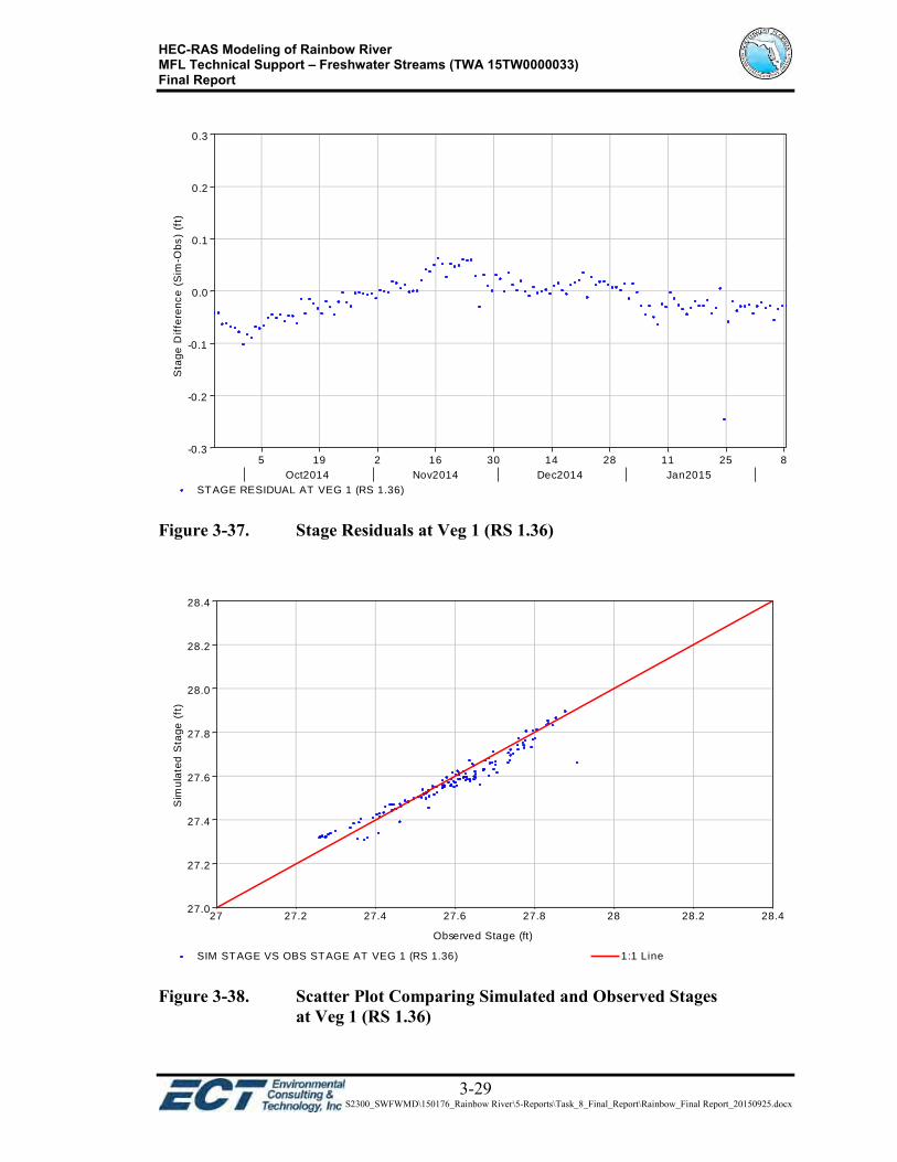
HEC-RAS Modeling of Rainbow River MFL Technical Support – Freshwater Streams (TWA 15TW0000033) Final Report
3-29 P:\S2300_SWFWMD\150176_Rainbow River\5-Reports\Task_8_Final_Report\Rainbow_Final Report_20150925.docx
Figure 3-37. Stage Residuals at Veg 1 (RS 1.36)
Figure 3-38. Scatter Plot Comparing Simulated and Observed Stages
at Veg 1 (RS 1.36)
5 19 2 16 30 14 28 11 25 8
Oct2014 Nov2014 Dec2014 Jan2015
Sta
ge
Dif
fere
nc
e (
Sim
-Ob
s)
(ft)
-0.3
-0.2
-0.1
0.0
0.1
0.2
0.3
STAGE RESIDUAL AT VEG 1 (RS 1.36)
Observed Stage (ft)
27 27.2 27.4 27.6 27.8 28 28.2 28.4
Sim
ula
ted
Sta
ge
(ft
)
27.0
27.2
27.4
27.6
27.8
28.0
28.2
28.4
SIM STAGE VS OBS STAGE AT VEG 1 (RS 1.36) 1:1 Line

HEC-RAS Modeling of Rainbow River MFL Technical Support – Freshwater Streams (TWA 15TW0000033) Final Report
3-30 P:\S2300_SWFWMD\150176_Rainbow River\5-Reports\Task_8_Final_Report\Rainbow_Final Report_20150925.docx
Figure 3-39. Scatter Plot Comparing Stage Residuals and Observed Stages
at Veg 1 (RS 1.36)
3.3.4 MODEL VERIFICATION
In addition to the model calibration performed using the long-term daily or real-time
stage data, miscellaneous stage data collected by USGS at the spring head and by
SWFWMD at a total of 11 vegetation transect sites was used to verify if the dynamic
HEC-RAS model is also able to predict reasonable water surface elevations at these
selected river sites. The stage datasets used in the model verification process are
summarized in Table 3-6.
The model verification results are graphically presented in Figures 3-40 through 3-43,
including plots of simulated stage hydrographs and observed stage data at the selected
river sites.
Review of the model verification results suggests most of the stage residuals fall within a
range of ±0.5 foot, except in the cases when accuracy of the measured stages is highly
questionable, e.g., the stage data collected in 2011 and the data in 2005 through 2007 at
Observed Stage (ft)
27.2 27.3 27.4 27.5 27.6 27.7 27.8 27.9
Sta
ge
Dif
fere
nc
e (
Sim
-Ob
s)
(ft)
-0.3
-0.2
-0.1
0.0
0.1
0.2
0.3
STAGE RESIDUAL VS OBS STAGE AT VEG 1 (RS 1.36)

HEC-RAS Modeling of Rainbow River MFL Technical Support – Freshwater Streams (TWA 15TW0000033) Final Report
3-31 P:\S2300_SWFWMD\150176_Rainbow River\5-Reports\Task_8_Final_Report\Rainbow_Final Report_20150925.docx
PHAB 1, PHAB Pool, and PHAB 2. A thorough quality control of the observed stage
data could eliminate these data errors and improve the model verification results.
Table 3–6. Summary of Stage Datasets Used in Model Verification
Station/Site Name Agency RS in HEC-RAS Start Date End Date Stage Data
Count
Rainbow River at Spring Head USGS 6.00 3/21/2005 1/31/2012 39
Veg 7 SWFWMD 5.77 7/1/2009 3/12/2015 34
Veg 6 SWFWMD 5.55 7/1/2009 3/12/2015 21
PHAB 1 SWFWMD 4.96 8/17/2005 3/12/2015 47
PHAB Pool SWFWMD 3.37 8/30/2005 3/12/2015 38
Veg 4 SWFWMD 3.25 7/1/2009 7/29/2009 3
PHAB 2 SWFWMD 3.09 8/11/2005 3/12/2015 46
Veg 3 SWFWMD 2.88 7/14/2009 3/12/2015 27
Veg 2.5 SWFWMD 2.66 7/1/2009 3/12/2015 31
Veg 2 SWFWMD 1.97 7/1/2009 3/12/2015 31
Veg 1 SWFWMD 1.36 7/1/2009 3/12/2015 40
Veg BBP SWFWMD 1.05 7/1/2009 3/12/2015 31
Figure 3-40. Simulated Stage Hydrographs and Observed Stage Data
at Spring Head, PHAB 1, PHAB Pool & PHAB 2
2005 2006 2007 2008 2009 2010 2011 2012 2013 2014
Sta
ge
(ft
)
26.5
27.0
27.5
28.0
28.5
29.0
29.5
30.0
30.5
31.0
31.5
SPRING HEAD OBS STAGE SPRING HEAD SIM STAGE (RS 6.00)
PHAB 1 OBS STAGE PHAB 1 SIM STAGE (RS 4.96)
PHAB POOL OBS STAGE PHAB POOL SIM STAGE (RS 3.37)
PHAB 2 OBS STAGE PHAB 2 SIM STAGE (RS 3.09)

HEC-RAS Modeling of Rainbow River MFL Technical Support – Freshwater Streams (TWA 15TW0000033) Final Report
3-32 P:\S2300_SWFWMD\150176_Rainbow River\5-Reports\Task_8_Final_Report\Rainbow_Final Report_20150925.docx
Figure 3-41. Simulated Stage Hydrographs and Observed Stage Data
at Veg 7, Veg 4 & Veg 2
Figure 3-42. Simulated Stage Hydrographs and Observed Stage Data
at Veg 6, Veg 3 & Veg 1
2009 2010 2011 2012 2013 2014
Sta
ge
(ft
)
26.0
26.5
27.0
27.5
28.0
28.5
29.0
29.5
30.0
30.5
VEG 7 OBS STAGE VEG 4 OBS STAGE VEG 2 OBS STAGE
VEG 7 SIM STAGE (RS 5.77) VEG 4 SIM STAGE (RS 3.25) VEG 2 SIM STAGE (RS 1.97)
2009 2010 2011 2012 2013 2014
Sta
ge
(ft
)
25.5
26.0
26.5
27.0
27.5
28.0
28.5
29.0
29.5
30.0
30.5
VEG 6 OBS STAGE VEG 3 OBS STAGE VEG 1 OBS STAGE
VEG 6 SIM STAGE (RS 5.55) VEG 3 SIM STAGE (RS 2.88) VEG 1 SIM STAGE (RS 1.36)

HEC-RAS Modeling of Rainbow River MFL Technical Support – Freshwater Streams (TWA 15TW0000033) Final Report
3-33 P:\S2300_SWFWMD\150176_Rainbow River\5-Reports\Task_8_Final_Report\Rainbow_Final Report_20150925.docx
Figure 3-43. Simulated Stage Hydrographs and Observed Stage Data
at Veg 2.5 & Veg BBP
3.4 SUMMARY OF DYNAMIC HEC-RAS MODEL CALIBRATION
In summary, a dynamic HEC-RAS model of Rainbow River has been developed and used
for dynamic flow analysis of a time period of 10 years from 3/11/2005 to 3/17/2015. The
stage data collected at various river sites were employed in the model calibration and
verification.
Upon review of the preliminary model calibration and verification results, it was
concluded that the model calibration task is accomplished and the HEC-RAS model
could be employed in the subsequent modeling of a series of District-provided MFLs
flow scenarios.
2009 2010 2011 2012 2013 2014
Sta
ge
(ft
)
25.5
26.0
26.5
27.0
27.5
28.0
28.5
VEG 2.5 OBS STAGE VEG BBP OBS STAGE VEG 2.5 SIM STAGE (RS 2.66)
VEG BBP SIM STAGE (RS 1.05)
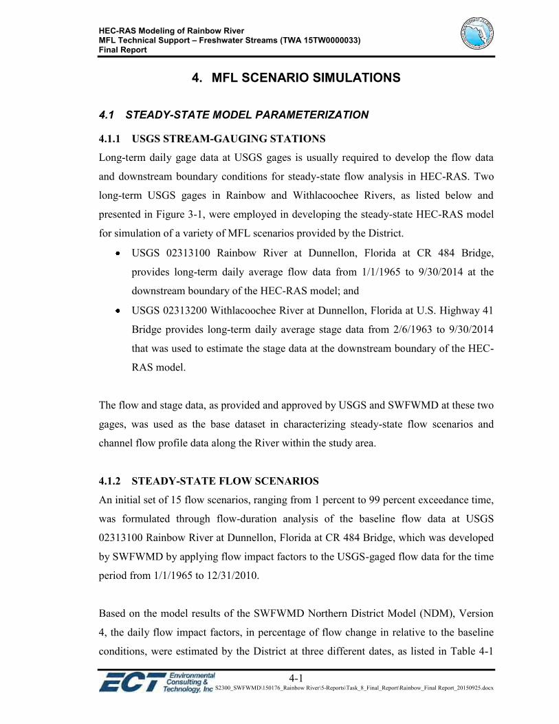
HEC-RAS Modeling of Rainbow River MFL Technical Support – Freshwater Streams (TWA 15TW0000033) Final Report
4-1 P:\S2300_SWFWMD\150176_Rainbow River\5-Reports\Task_8_Final_Report\Rainbow_Final Report_20150925.docx
4. MFL SCENARIO SIMULATIONS
4.1 STEADY-STATE MODEL PARAMETERIZATION
4.1.1 USGS STREAM-GAUGING STATIONS
Long-term daily gage data at USGS gages is usually required to develop the flow data
and downstream boundary conditions for steady-state flow analysis in HEC-RAS. Two
long-term USGS gages in Rainbow and Withlacoochee Rivers, as listed below and
presented in Figure 3-1, were employed in developing the steady-state HEC-RAS model
for simulation of a variety of MFL scenarios provided by the District.
USGS 02313100 Rainbow River at Dunnellon, Florida at CR 484 Bridge,
provides long-term daily average flow data from 1/1/1965 to 9/30/2014 at the
downstream boundary of the HEC-RAS model; and
USGS 02313200 Withlacoochee River at Dunnellon, Florida at U.S. Highway 41
Bridge provides long-term daily average stage data from 2/6/1963 to 9/30/2014
that was used to estimate the stage data at the downstream boundary of the HEC-
RAS model.
The flow and stage data, as provided and approved by USGS and SWFWMD at these two
gages, was used as the base dataset in characterizing steady-state flow scenarios and
channel flow profile data along the River within the study area.
4.1.2 STEADY-STATE FLOW SCENARIOS
An initial set of 15 flow scenarios, ranging from 1 percent to 99 percent exceedance time,
was formulated through flow-duration analysis of the baseline flow data at USGS
02313100 Rainbow River at Dunnellon, Florida at CR 484 Bridge, which was developed
by SWFWMD by applying flow impact factors to the USGS-gaged flow data for the time
period from 1/1/1965 to 12/31/2010.
Based on the model results of the SWFWMD Northern District Model (NDM), Version
4, the daily flow impact factors, in percentage of flow change in relative to the baseline
conditions, were estimated by the District at three different dates, as listed in Table 4-1

HEC-RAS Modeling of Rainbow River MFL Technical Support – Freshwater Streams (TWA 15TW0000033) Final Report
4-2 P:\S2300_SWFWMD\150176_Rainbow River\5-Reports\Task_8_Final_Report\Rainbow_Final Report_20150925.docx
below, representing the baseline conditions in 1965 and the post-development conditions
in 1995 and 2010. A linear interpolation approach was used to generate the daily flow
impact factor for each day in between 1/1/1965 and 12/31/2010.
The resultant baseline flow data and flow-duration curve are graphically presented in
Figures 4-1 and 4-2. The 15 flow scenarios, as summarized in Table 4-2, cover a wide
range of flow conditions, from extreme low, average, to high flow.
Table 4–1. Summary of Flow Impact Factors at USGS 02313100
ID Date Daily Flow Impact Factor in Percent of Flow Change
1 1/1/1965 0.0
2 12/31/1995 1.1
3 12/31/2010 1.7
Data Source: SWFWMD, 2015.
Figure 4-1. Baseline Flow Data at USGS 02313100
1965 1970 1975 1980 1985 1990 1995 2000 2005 2010
Flo
w (
cfs
)
400
500
600
700
800
900
1,000
1,100
usgs 02313100 @ CR484 BRIDGE - Baseline Flow
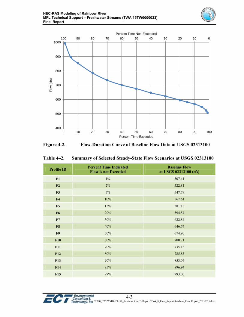
HEC-RAS Modeling of Rainbow River MFL Technical Support – Freshwater Streams (TWA 15TW0000033) Final Report
4-3 P:\S2300_SWFWMD\150176_Rainbow River\5-Reports\Task_8_Final_Report\Rainbow_Final Report_20150925.docx
Figure 4-2. Flow-Duration Curve of Baseline Flow Data at USGS 02313100 Table 4–2. Summary of Selected Steady-State Flow Scenarios at USGS 02313100
Profile ID Percent Time Indicated Flow is not Exceeded
Baseline Flow at USGS 02313100 (cfs)
F1 1% 507.41
F2 2% 522.81
F3 5% 547.79
F4 10% 567.61
F5 15% 581.18
F6 20% 594.54
F7 30% 622.84
F8 40% 646.74
F9 50% 674.90
F10 60% 700.71
F11 70% 735.18
F12 80% 785.85
F13 90% 853.04
F14 95% 896.94
F15 99% 993.00
0 10 20 30 40 50 60 70 80 90 100
400
500
600
700
800
900
1000
0 10 20 30 40 50 60 70 80 90 100
Percent Time Non-Exceeded
Flo
w (
cfs
)
Percent Time Exceeded

HEC-RAS Modeling of Rainbow River MFL Technical Support – Freshwater Streams (TWA 15TW0000033) Final Report
4-4 P:\S2300_SWFWMD\150176_Rainbow River\5-Reports\Task_8_Final_Report\Rainbow_Final Report_20150925.docx
4.1.3 CHANNEL FLOW PROFILES
A channel flow profile analysis has been previously developed at the study river reach, as
documented in Section 2.3.1. Utilizing the methodology and results of the channel flow
profile analysis, flow rates for all given steady-state flow scenarios were estimated for
each of the cross-sections in the HEC-RAS model.
4.1.4 DOWNSTREAM BOUNDARY CONDITIONS
As described in Section 2.3.3, the downstream boundary conditions at USGS 02313100
Rainbow River at Dunnellon, Florida have been defined to run a steady-state flow
analysis for the preliminary HEC-RAS model. The methodology used in developing the
downstream boundary conditions was described in Section 2.3.2. For a given MFL
scenario to be simulated in HEC-RAS, two independent variables - Flow in Rainbow
River and Stage in Withlacoochee River, have to be defined prior to estimating a stage
boundary condition at CR 484 Bridge using the multiple regression method (Figure 2-7).
Similar to the flow-duration analysis performed for the baseline flow data at USGS
02313100 at CR 484 Bridge, a stage-duration analysis was conducted for the stage data at
USGS 02313200 at US 41 Bridge, for a period from 1/1/1965 through 12/31/2010
(Figure 4-3). The resultant stage-duration curve is plotted in Figure 4-4 and a total of 15
steady-state stage scenarios were formulated as listed in Table 4-3.
By applying the multiple regression curve (Figure 2-7), a matrix of downstream boundary
conditions, including a total of 225 stage values, were estimated at USGS 02313100 at
CR 484 Bridge, as summarized in Table 4-4.

HEC-RAS Modeling of Rainbow River MFL Technical Support – Freshwater Streams (TWA 15TW0000033) Final Report
4-5 P:\S2300_SWFWMD\150176_Rainbow River\5-Reports\Task_8_Final_Report\Rainbow_Final Report_20150925.docx
Figure 4-3. Historic Stage Data at USGS 02313200
Figure 4-4. Stage-Duration Curve at USGS 02313200
1965 1970 1975 1980 1985 1990 1995 2000 2005 2010
Sta
ge
(ft
-NA
VD
)
22
23
24
25
26
27
28
29
30
USGS 02313200 @ US 41 BRIDGE - Stage
0 10 20 30 40 50 60 70 80 90 100
25.0
25.5
26.0
26.5
27.0
27.5
28.0
28.5
0 10 20 30 40 50 60 70 80 90 100
Percent Time Non-Exceeded
Sta
ge (
ft-N
AV
D)
Percent Time Exceeded

HEC-RAS Modeling of Rainbow River MFL Technical Support – Freshwater Streams (TWA 15TW0000033) Final Report
4-6 P:\S2300_SWFWMD\150176_Rainbow River\5-Reports\Task_8_Final_Report\Rainbow_Final Report_20150925.docx
Table 4–3. Summary of Selected Steady-State Stage Scenarios at USGS 02313200
Profile ID Percent Time Indicated Stage is not Exceeded
Stage at USGS 02313200 (ft-NAVD)
S1 1% 25.09
S2 1.25% 25.98
S3 1.5% 26.18
S4 1.75% 26.31
S5 2% 26.37
S6 3% 26.60
S7 5% 26.72
S8 10% 26.80
S9 25% 26.92
S10 50% 27.07
S11 75% 27.30
S12 85% 27.49
S13 90% 27.60
S14 95% 27.82
S15 99% 28.36

HEC-RAS Modeling of Rainbow River MFL Technical Support – Freshwater Streams (TWA 15TW0000033) Final Report
4-7 P:\S2300_SWFWMD\150176_Rainbow River\5-Reports\Task_8_Final_Report\Rainbow_Final Report_20150925.docx
Table 4–4. Summary of Downstream Boundary Conditions – Stages at USGS 02313100 Using Multiple Regression Curve
ID
Percent Time Indicated
Flow is not Exceeded
Flow at USGS
02313100 (cfs)
Downstream Boundary Conditions – Stage at USGS 02313100 (ft-NAVD) With Selected Steady-State Stage Scenarios at USGS 02313200, Stage in ft-NAVD
S1 S2 S3 S4 S5 S6 S7 S8 S9 S10 S11 S12 S13 S14 S15 1% 1.25% 1.5% 1.75% 2% 3% 5% 10% 25% 50% 75% 85% 90% 95% 99%
25.09 25.98 26.18 26.31 26.37 26.60 26.72 26.80 26.92 27.07 27.30 27.49 27.60 27.82 28.36
F1 1% 507.41 25.20 26.11 26.31 26.44 26.51 26.74 26.86 26.94 27.07 27.22 27.45 27.65 27.76 27.98 28.53
F2 2% 522.81 25.20 26.11 26.31 26.44 26.51 26.74 26.86 26.94 27.07 27.22 27.45 27.64 27.76 27.98 28.53
F3 5% 547.79 25.20 26.11 26.31 26.44 26.51 26.74 26.86 26.94 27.07 27.22 27.45 27.64 27.76 27.98 28.53
F4 10% 567.61 25.20 26.11 26.31 26.45 26.51 26.74 26.86 26.94 27.07 27.22 27.45 27.65 27.76 27.98 28.53
F5 15% 581.18 25.21 26.11 26.32 26.45 26.51 26.74 26.87 26.95 27.07 27.22 27.46 27.65 27.76 27.98 28.54
F6 20% 594.54 25.21 26.12 26.32 26.45 26.51 26.75 26.87 26.95 27.07 27.23 27.46 27.65 27.76 27.99 28.54
F7 30% 622.84 25.22 26.13 26.33 26.46 26.53 26.76 26.88 26.96 27.09 27.24 27.47 27.67 27.78 28.00 28.55
F8 40% 646.74 25.24 26.15 26.35 26.48 26.54 26.78 26.90 26.98 27.10 27.26 27.49 27.68 27.79 28.02 28.57
F9 50% 674.90 25.27 26.18 26.38 26.51 26.57 26.81 26.93 27.01 27.13 27.29 27.52 27.71 27.82 28.05 28.60
F10 60% 700.71 25.31 26.21 26.42 26.55 26.61 26.85 26.97 27.05 27.17 27.32 27.56 27.75 27.86 28.08 28.64
F11 70% 735.18 25.38 26.28 26.49 26.62 26.68 26.91 27.03 27.12 27.24 27.39 27.62 27.82 27.93 28.15 28.70
F12 80% 785.85 25.52 26.43 26.63 26.76 26.82 27.06 27.18 27.26 27.38 27.53 27.77 27.96 28.07 28.30 28.85
F13 90% 853.04 25.80 26.71 26.91 27.04 27.11 27.34 27.46 27.54 27.67 27.82 28.05 28.24 28.36 28.58 29.13
F14 95% 896.94 26.06 26.97 27.17 27.30 27.36 27.60 27.72 27.80 27.92 28.07 28.31 28.50 28.61 28.84 29.39
F15 99% 993.00 26.85 27.76 27.96 28.09 28.15 28.39 28.51 28.59 28.71 28.86 29.10 29.29 29.40 29.63 30.18

HEC-RAS Modeling of Rainbow River MFL Technical Support – Freshwater Streams (TWA 15TW0000033) Final Report
4-8 P:\S2300_SWFWMD\150176_Rainbow River\5-Reports\Task_8_Final_Report\Rainbow_Final Report_20150925.docx
4.2 STEADY-STATE MODEL SIMULATION
4.2.1 MODEL SIMULATION
The channel flow profiles and downstream boundary conditions for the 225 steady-state
scenarios were developed and stored in an Excel spreadsheet prior to being imported into
the HEC-RAS model.
4.2.2 SIMULATION RESULTS
A good collection of post-processing tools are available in HEC-RAS to review model
output data in both tabular and graphic views, including stage profile plot, cross-section
plot, profile output table, x-y-z perspective plot, etc. Using these post-processing tools,
the hydraulic characteristics of the cross-sections (e.g., water surface elevation, average
depth, top surface width, wetted perimeter, and shear stress), could be reviewed in HEC-
RAS. The model output data could also be exported to GIS files and/or customized
reports. The followings are three commonly used post-processing tools for model output
review:
Stage Profile Plot
The stage profile plot could be used to check the overall water elevation profile shape for
a given steady-state scenario and be zoomed in to identify the type of flow profile (e.g.,
M1 profile), within a small river segment. An example stage profile plot is presented in
Figure 4-5, illustrating a total of 15 steady-state flow scenarios (F1 through F15) in
Rainbow River at a 50 percentile (P50) stage scenario (S10) in Withlacoochee River. For
comparison purposes, Figure 4-6 illustrates the stage profile plot for a total of 15 steady-
state stage scenarios (S1 through S15) in Withlacoochee River at a P50 flow scenario
(F9) in Rainbow River.
Cross-Section Plot
The cross-section plot is another useful tool to check water depth and flow (velocity)
distribution within the main channel or floodplain of a cross-section for a given scenario.
A cross-section is allowed to be divided into up to 45 subsections and the output data of
each subsection can be presented in both tabular and graphic formats in HEC-RAS.

HEC-RAS Modeling of Rainbow River MFL Technical Support – Freshwater Streams (TWA 15TW0000033) Final Report
4-9 P:\S2300_SWFWMD\150176_Rainbow River\5-Reports\Task_8_Final_Report\Rainbow_Final Report_20150925.docx
A sample cross-section plot is presented in Figure 4-7, at one of the SWFWMD river site
Veg 1 or RS 1.36. The main channel at this cross-section was evenly subdivided into 43
subsections and the flow distribution in the main channel is symbolized in graduated
colors based on the flow velocity magnitude calculated in each subsection.
Profile Output Table
An example profile output table is presented in Figure 4-8, showing one of the standard
tables for model output data review. The model output data summarized in the profile
output tables, including water surface elevation and total flow, could be exported to an
Excel spreadsheet for additional data processing, analysis, and presentation.
Figures 4-9 and 4-10 illustrate the stage-flow rating curves developed at the SWFWMD
river sites Veg 1 and PHAB 1, respectively, based on the model output data of the 225
steady-state scenarios. Similar stage-flow rating curves could be developed for other
cross-sections in the HEC-RAS model, and be used to assess which is the predominant
variable in determining the water surface elevations at a specific cross-section or river
site, between the flow in Rainbow River and the stage in Withlacoochee River.
For example at the river site Veg 1 at RS 1.36 (Figure 3-1), review of the resultant stage-
flow rating curves in Figure 4-9 suggests the stage in Withlacoochee River is the major
factor controlling the water surface elevations at this site. This conclusion is also
supported by the historic USGS gage data as well as the field observations of the severe
backwater effects (zero or reverse flow) from the downstream Withlacoochee River,
particularly in the river segment downstream of the rocky shoal near RS 3.10.
The stage-flow rating curves for the river site PHAB 1 at RS 4.96 (Figure 3-1), as plotted
in Figure 4-10, indicate much less backwater effects at this location compared to the
downstream river site Veg 1 at RS 1.36. The flow from Rainbow River appears to be the
predominant factor controlling the surface water elevations at this location.

HEC-RAS Modeling of Rainbow River MFL Technical Support – Freshwater Streams (TWA 15TW0000033) Final Report
4-10 P:\S2300_SWFWMD\150176_Rainbow River\5-Reports\Task_8_Final_Report\Rainbow_Final Report_20150925.docx
Figure 4-5. Stage Profile Plot of 15 Flow Scenarios in Rainbow River with P50 Stage Scenario (S10) in Withlacoochee River
0 5000 10000 15000 20000 25000 3000010
15
20
25
30
35
Rainbow_V3 Plan: Rainbow_V3_SS_RF 8/11/2015
Main Channel Distance (ft)
Ele
vation
(ft)
Legend
WS F15S10
WS F14S10
WS F13S10
WS F12S10
WS F11S10
WS F10S10
WS F9S10
WS F8S10
WS F7S10
WS F6S10
WS F5S10
WS F4S10
WS F3S10
WS F2S10
WS F1S10
Ground
1.0
01
.09
1.1
81
.28
1.3
6
1.4
61
.56
1.6
51
.74
1.8
41
.93
2.0
2
2.1
22
.21
2.3
0
2.4
02
.49
2.5
82
.66
2.7
72
.86
2.9
63
.05
3.1
4
3.2
33
.33
3.4
2
3.5
13
.61
3.7
0
3.7
93
.89
3.9
84
.07
4.1
74
.26
4.3
5
4.4
54
.54
4.6
3
4.7
34
.82
4.9
1
5.0
15
.10
5.1
9
5.2
95
.38
5.4
7
5.5
75
.66
5.7
5
5.8
45
.94
Rainbow Main

HEC-RAS Modeling of Rainbow River MFL Technical Support – Freshwater Streams (TWA 15TW0000033) Final Report
4-11 P:\S2300_SWFWMD\150176_Rainbow River\5-Reports\Task_8_Final_Report\Rainbow_Final Report_20150925.docx
Figure 4-6. Stage Profile Plot of 15 Stage Scenarios in Withlacoochee River with P50 Flow Scenario (F9) in Rainbow River
0 5000 10000 15000 20000 25000 3000010
15
20
25
30
35
Rainbow_V3 Plan: Rainbow_V3_SS_RF 8/11/2015
Main Channel Distance (ft)
Ele
vation
(ft)
Legend
WS F9S15
WS F9S14
WS F9S13
WS F9S12
WS F9S11
WS F9S10
WS F9S9
WS F9S8
WS F9S7
WS F9S6
WS F9S5
WS F9S4
WS F9S3
WS F9S2
WS F9S1
Ground
1.0
01
.09
1.1
81
.28
1.3
6
1.4
61
.56
1.6
51
.74
1.8
4
1.9
32
.02
2.1
22
.21
2.3
0
2.4
02
.49
2.5
82
.68
2.7
7
2.8
62
.96
3.0
5
3.1
43
.23
3.3
33
.42
3.5
1
3.6
13
.70
3.7
93
.89
3.9
8
4.0
74
.17
4.2
6
4.3
54
.45
4.5
44
.63
4.7
3
4.8
24
.91
5.0
15
.10
5.1
9
5.2
95
.38
5.4
75
.55
5.6
6
5.7
55
.84
5.9
4
Rainbow Main

HEC-RAS Modeling of Rainbow River MFL Technical Support – Freshwater Streams (TWA 15TW0000033) Final Report
4-12 P:\S2300_SWFWMD\150176_Rainbow River\5-Reports\Task_8_Final_Report\Rainbow_Final Report_20150925.docx
Figure 4-7. Cross-Section Plot at Veg 1 (RS 1.36) for P50 Flow Scenario (F9) in Rainbow River and P50 Stage Scenario (S10) in Withlacoochee River
Figure 4-8. Profile Output Table for Steady-State HEC-RAS Model Output Review
250 300 350 400 450
15
20
25
30
Rainbow_V3 Pl an: Rainbow_V3_SS_RF 8/11/2015 RS = 1.36 Section: Veg 1 Source: 2008 Veg Transect Survey
Station (ft)
Ele
vation
(ft)
Legend
WS F9S10
0.0 ft/s
0.1 ft/s
0.2 ft/s
0.3 ft/s
0.4 ft/s
0.5 ft/s
0.6 ft/s
Ground
Bank Sta
.22 .033 .22
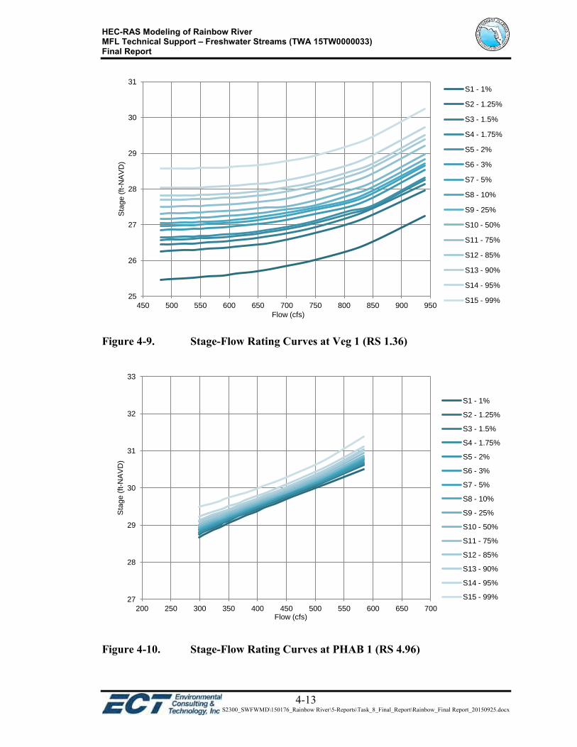
HEC-RAS Modeling of Rainbow River MFL Technical Support – Freshwater Streams (TWA 15TW0000033) Final Report
4-13 P:\S2300_SWFWMD\150176_Rainbow River\5-Reports\Task_8_Final_Report\Rainbow_Final Report_20150925.docx
Figure 4-9. Stage-Flow Rating Curves at Veg 1 (RS 1.36)
Figure 4-10. Stage-Flow Rating Curves at PHAB 1 (RS 4.96)
25
26
27
28
29
30
31
450 500 550 600 650 700 750 800 850 900 950
Sta
ge (
ft-N
AV
D)
Flow (cfs)
S1 - 1%
S2 - 1.25%
S3 - 1.5%
S4 - 1.75%
S5 - 2%
S6 - 3%
S7 - 5%
S8 - 10%
S9 - 25%
S10 - 50%
S11 - 75%
S12 - 85%
S13 - 90%
S14 - 95%
S15 - 99%
27
28
29
30
31
32
33
200 250 300 350 400 450 500 550 600 650 700
Sta
ge
(ft-N
AV
D)
Flow (cfs)
S1 - 1%
S2 - 1.25%
S3 - 1.5%
S4 - 1.75%
S5 - 2%
S6 - 3%
S7 - 5%
S8 - 10%
S9 - 25%
S10 - 50%
S11 - 75%
S12 - 85%
S13 - 90%
S14 - 95%
S15 - 99%
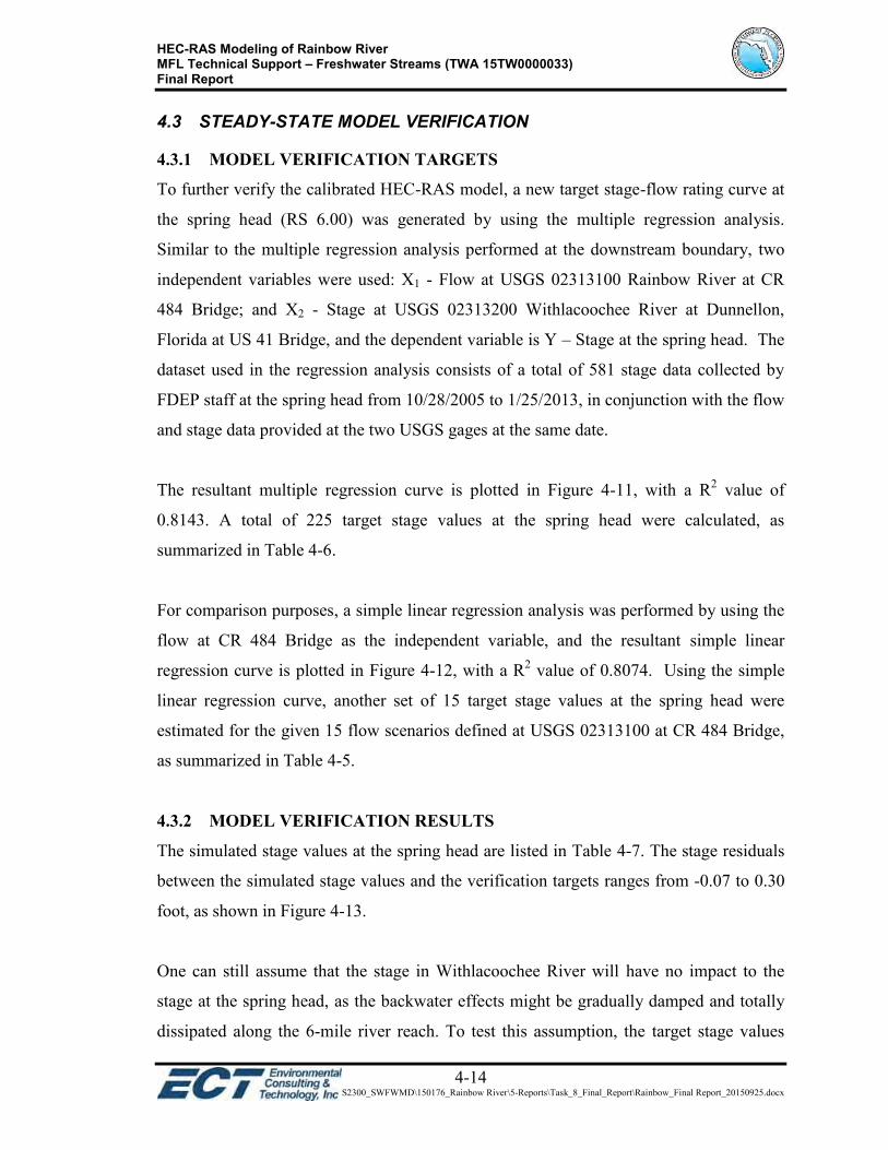
HEC-RAS Modeling of Rainbow River MFL Technical Support – Freshwater Streams (TWA 15TW0000033) Final Report
4-14 P:\S2300_SWFWMD\150176_Rainbow River\5-Reports\Task_8_Final_Report\Rainbow_Final Report_20150925.docx
4.3 STEADY-STATE MODEL VERIFICATION
4.3.1 MODEL VERIFICATION TARGETS
To further verify the calibrated HEC-RAS model, a new target stage-flow rating curve at
the spring head (RS 6.00) was generated by using the multiple regression analysis.
Similar to the multiple regression analysis performed at the downstream boundary, two
independent variables were used: X1 - Flow at USGS 02313100 Rainbow River at CR
484 Bridge; and X2 - Stage at USGS 02313200 Withlacoochee River at Dunnellon,
Florida at US 41 Bridge, and the dependent variable is Y – Stage at the spring head. The
dataset used in the regression analysis consists of a total of 581 stage data collected by
FDEP staff at the spring head from 10/28/2005 to 1/25/2013, in conjunction with the flow
and stage data provided at the two USGS gages at the same date.
The resultant multiple regression curve is plotted in Figure 4-11, with a R2 value of
0.8143. A total of 225 target stage values at the spring head were calculated, as
summarized in Table 4-6.
For comparison purposes, a simple linear regression analysis was performed by using the
flow at CR 484 Bridge as the independent variable, and the resultant simple linear
regression curve is plotted in Figure 4-12, with a R2 value of 0.8074. Using the simple
linear regression curve, another set of 15 target stage values at the spring head were
estimated for the given 15 flow scenarios defined at USGS 02313100 at CR 484 Bridge,
as summarized in Table 4-5.
4.3.2 MODEL VERIFICATION RESULTS
The simulated stage values at the spring head are listed in Table 4-7. The stage residuals
between the simulated stage values and the verification targets ranges from -0.07 to 0.30
foot, as shown in Figure 4-13.
One can still assume that the stage in Withlacoochee River will have no impact to the
stage at the spring head, as the backwater effects might be gradually damped and totally
dissipated along the 6-mile river reach. To test this assumption, the target stage values

HEC-RAS Modeling of Rainbow River MFL Technical Support – Freshwater Streams (TWA 15TW0000033) Final Report
4-15 P:\S2300_SWFWMD\150176_Rainbow River\5-Reports\Task_8_Final_Report\Rainbow_Final Report_20150925.docx
estimated by the simple linear stage-flow rating curve (Table 4-5 and Figure 4-12) were
used to substitute the verification targets listed in Table 4-6. As presented in Figure 4-14,
the stage residuals range from -0.30 to 0.41 foot, which almost doubles the range when
using the multiple regression curve (Figure 4-13). Obviously, the simple linear regression
curve based on the assumption of zero backwater effects is not as successful as the
multiple regression curve in terms of model verification results. Therefore, the stage at
the spring head appears to be influenced by the stage in Withlacoochee River, to a certain
extent, while significant influence of backwater effect was observed in the lower portion
of the River.
Figure 4-11. Multiple Regression Curve at Spring Head (RS 6.00)

HEC-RAS Modeling of Rainbow River MFL Technical Support – Freshwater Streams (TWA 15TW0000033) Final Report
4-16 P:\S2300_SWFWMD\150176_Rainbow River\5-Reports\Task_8_Final_Report\Rainbow_Final Report_20150925.docx
Figure 4-12. Simple Linear Regression Curve at Spring Head (RS 6.00) Table 4–5. Summary of Model Verification Targets - Simple Linear Regression
Curve
ID Percent Time Indicated Flow is not Exceeded
Baseline Flow at USGS 02313100 (cfs)
Model Verification Targets Stage at Spring Head (ft-NAVD)
F1 1% 507.41 29.46
F2 2% 522.81 29.53
F3 5% 547.79 29.64
F4 10% 567.61 29.72
F5 15% 581.18 29.78
F6 20% 594.54 29.84
F7 30% 622.84 29.96
F8 40% 646.74 30.06
F9 50% 674.90 30.18
F10 60% 700.71 30.30
F11 70% 735.18 30.44
F12 80% 785.85 30.66
F13 90% 853.04 30.95
F14 95% 896.94 31.14
F15 99% 993.00 31.55
HEC-RAS Modeling of Rainbow River MFL Technical Support – Freshwater Streams (TWA 15TW0000033) Final Report
4-17 P:\S2300_SWFWMD\150176_Rainbow River\5-Reports\Task_8_Final_Report\Rainbow_Final Report_20150925.docx
4.4 SUMMARY OF MFL SCENARIO SIMULATIONS
In summary, a steady-state HEC-RAS model of Rainbow River was developed on the
basis of the dynamic HEC-RAS model previously developed and calibrated in Section 3.
Steady-state flow analysis was conducted for each of the 225 steady-state or MFL
scenarios that represent the combinations of the 15 flow scenarios in Rainbow River and
the 15 stage scenarios in Withlacoochee River.
Review of the model simulation and verification results suggests that the MFL Scenario
Simulations task is successfully accomplished and the steady-state HEC-RAS model
could be utilized in the subsequent ecological analysis and ultimately MFLs
establishment in Rainbow River by the District.

HEC-RAS Modeling of Rainbow River MFL Technical Support – Freshwater Streams (TWA 15TW0000033) Final Report
4-18 P:\S2300_SWFWMD\150176_Rainbow River\5-Reports\Task_8_Final_Report\Rainbow_Final Report_20150925.docx
Table 4–6. Summary of Model Verification Targets - Multiple Regression Curve
ID
Percent Time Indicated
Flow is not Exceeded
Baseline Flow at USGS
02313100 (cfs)
Model Verification Targets - Stage at Spring Head (ft-NAVD) With Selected Steady-State Stage Scenarios at USGS 02313200, Stage in ft-NAVD
S1 S2 S3 S4 S5 S6 S7 S8 S9 S10 S11 S12 S13 S14 S15
1% 1.25% 1.5% 1.75% 2% 3% 5% 10% 25% 50% 75% 85% 90% 95% 99%
25.09 25.98 26.18 26.31 26.37 26.60 26.72 26.80 26.92 27.07 27.30 27.49 27.60 27.82 28.36
F1 1% 507.41 29.31 29.39 29.40 29.41 29.42 29.44 29.45 29.45 29.46 29.48 29.50 29.51 29.52 29.54 29.59
F2 2% 522.81 29.37 29.45 29.47 29.48 29.48 29.50 29.51 29.52 29.53 29.54 29.56 29.58 29.59 29.60 29.65
F3 5% 547.79 29.48 29.55 29.57 29.58 29.58 29.60 29.61 29.62 29.63 29.64 29.66 29.68 29.69 29.71 29.75
F4 10% 567.61 29.56 29.63 29.65 29.66 29.67 29.69 29.70 29.70 29.71 29.72 29.74 29.76 29.77 29.79 29.83
F5 15% 581.18 29.61 29.69 29.71 29.72 29.72 29.74 29.75 29.76 29.77 29.78 29.80 29.82 29.83 29.84 29.89
F6 20% 594.54 29.67 29.74 29.76 29.77 29.78 29.80 29.81 29.81 29.82 29.84 29.86 29.87 29.88 29.90 29.95
F7 30% 622.84 29.78 29.86 29.88 29.89 29.89 29.91 29.92 29.93 29.94 29.95 29.97 29.99 30.00 30.02 30.06
F8 40% 646.74 29.88 29.96 29.97 29.99 29.99 30.01 30.02 30.03 30.04 30.05 30.07 30.09 30.10 30.11 30.16
F9 50% 674.90 30.00 30.07 30.09 30.10 30.11 30.13 30.14 30.14 30.15 30.17 30.19 30.20 30.21 30.23 30.28
F10 60% 700.71 30.10 30.18 30.20 30.21 30.21 30.23 30.24 30.25 30.26 30.27 30.29 30.31 30.32 30.34 30.38
F11 70% 735.18 30.25 30.32 30.34 30.35 30.35 30.37 30.38 30.39 30.40 30.41 30.43 30.45 30.46 30.48 30.52
F12 80% 785.85 30.45 30.53 30.55 30.56 30.56 30.58 30.59 30.60 30.61 30.62 30.64 30.66 30.67 30.69 30.73
F13 90% 853.04 30.73 30.81 30.82 30.83 30.84 30.86 30.87 30.87 30.89 30.90 30.92 30.93 30.94 30.96 31.01
F14 95% 896.94 30.91 30.99 31.00 31.01 31.02 31.04 31.05 31.06 31.07 31.08 31.10 31.11 31.12 31.14 31.19
F15 99% 993.00 31.30 31.38 31.40 31.41 31.41 31.43 31.44 31.45 31.46 31.47 31.49 31.51 31.52 31.54 31.58

HEC-RAS Modeling of Rainbow River MFL Technical Support – Freshwater Streams (TWA 15TW0000033) Final Report
4-19 P:\S2300_SWFWMD\150176_Rainbow River\5-Reports\Task_8_Final_Report\Rainbow_Final Report_20150925.docx
Table 4–7. Summary of Model Simulation Results – Stage at Spring Head (RS 6.00)
ID
Percent Time Indicated
Flow is not Exceeded
Baseline Flow at USGS
02313100 (cfs)
Model Simulation Results - Stage at Spring Head (ft-NAVD) With Selected Steady-State Stage Scenarios at USGS 02313200, Stage in ft-NAVD
S1 S2 S3 S4 S5 S6 S7 S8 S9 S10 S11 S12 S13 S14 S15
1% 1.25% 1.5% 1.75% 2% 3% 5% 10% 25% 50% 75% 85% 90% 95% 99%
25.09 25.98 26.18 26.31 26.37 26.60 26.72 26.80 26.92 27.07 27.30 27.49 27.60 27.82 28.36
F1 1% 507.41 29.27 29.32 29.34 29.36 29.37 29.4 29.42 29.43 29.45 29.48 29.53 29.57 29.6 29.67 29.87
F2 2% 522.81 29.35 29.4 29.42 29.43 29.44 29.47 29.49 29.5 29.52 29.55 29.59 29.64 29.67 29.73 29.93
F3 5% 547.79 29.47 29.52 29.54 29.55 29.56 29.59 29.61 29.62 29.64 29.66 29.7 29.74 29.77 29.83 30.02
F4 10% 567.61 29.57 29.62 29.63 29.65 29.65 29.68 29.69 29.71 29.72 29.75 29.78 29.82 29.85 29.91 30.09
F5 15% 581.18 29.63 29.68 29.7 29.71 29.71 29.74 29.76 29.77 29.78 29.81 29.84 29.88 29.9 29.96 30.14
F6 20% 594.54 29.7 29.74 29.76 29.77 29.77 29.8 29.81 29.82 29.84 29.86 29.89 29.93 29.96 30.01 30.18
F7 30% 622.84 29.82 29.87 29.88 29.89 29.9 29.92 29.93 29.94 29.96 29.98 30.01 30.05 30.07 30.12 30.28
F8 40% 646.74 29.93 29.97 29.98 29.99 30 30.02 30.03 30.04 30.06 30.08 30.11 30.14 30.16 30.21 30.37
F9 50% 674.90 30.05 30.08 30.1 30.11 30.11 30.13 30.15 30.16 30.17 30.19 30.22 30.25 30.27 30.32 30.47
F10 60% 700.71 30.15 30.19 30.2 30.21 30.22 30.24 30.25 30.26 30.27 30.29 30.32 30.35 30.37 30.42 30.57
F11 70% 735.18 30.29 30.33 30.34 30.35 30.36 30.38 30.39 30.4 30.41 30.42 30.46 30.49 30.51 30.56 30.7
F12 80% 785.85 30.49 30.53 30.54 30.55 30.55 30.58 30.59 30.6 30.6 30.62 30.66 30.69 30.71 30.76 30.9
F13 90% 853.04 30.74 30.78 30.8 30.81 30.81 30.83 30.84 30.85 30.87 30.89 30.92 30.96 30.98 31.03 31.18
F14 95% 896.94 30.9 30.95 30.96 30.97 30.97 31 31.02 31.03 31.04 31.07 31.11 31.15 31.17 31.22 31.38
F15 99% 993.00 31.25 31.32 31.34 31.36 31.37 31.41 31.43 31.44 31.47 31.5 31.56 31.61 31.61 31.67 31.88

HEC-RAS Modeling of Rainbow River MFL Technical Support – Freshwater Streams (TWA 15TW0000033) Final Report
4-20 P:\S2300_SWFWMD\150176_Rainbow River\5-Reports\Task_8_Final_Report\Rainbow_Final Report_20150925.docx
Figure 4-13. Stage Residuals at Spring Head (RS 6.00) Using Multiple Regression Curve
-0.5
-0.4
-0.3
-0.2
-0.1
0
0.1
0.2
0.3
0.4
0.5
S1 S2 S3 S4 S5 S6 S7 S8 S9 S10 S11 S12 S13 S14 S15
Sta
ge
Diffe
ren
ce
(ft
)
F1
F2
F3
F4
F5
F6
F7
F8
F9
F10
F11
F12
F13
F14
F15
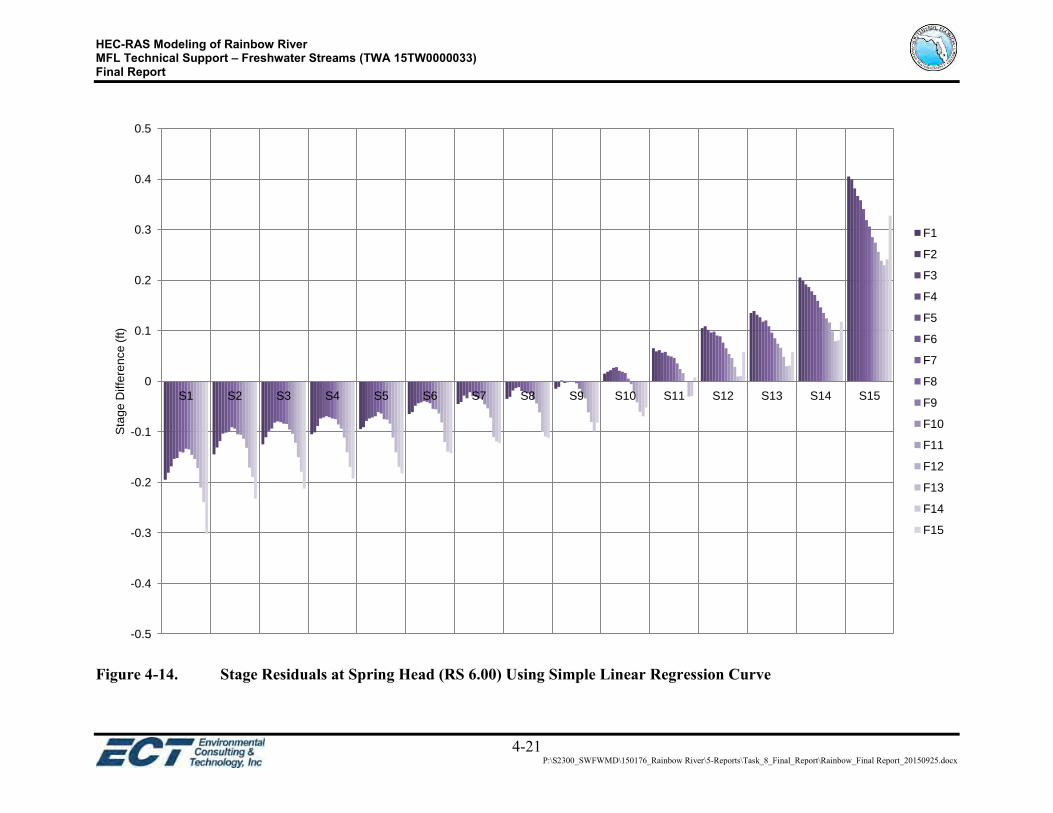
HEC-RAS Modeling of Rainbow River MFL Technical Support – Freshwater Streams (TWA 15TW0000033) Final Report
4-21 P:\S2300_SWFWMD\150176_Rainbow River\5-Reports\Task_8_Final_Report\Rainbow_Final Report_20150925.docx
Figure 4-14. Stage Residuals at Spring Head (RS 6.00) Using Simple Linear Regression Curve
-0.5
-0.4
-0.3
-0.2
-0.1
0
0.1
0.2
0.3
0.4
0.5
S1 S2 S3 S4 S5 S6 S7 S8 S9 S10 S11 S12 S13 S14 S15
Sta
ge
Diffe
ren
ce
(ft
)
F1
F2
F3
F4
F5
F6
F7
F8
F9
F10
F11
F12
F13
F14
F15

HEC-RAS Modeling of Rainbow River MFL Technical Support – Freshwater Streams (TWA 15TW0000033) Final Report
5-1 P:\S2300_SWFWMD\150176_Rainbow River\5-Reports\Task_8_Final_Report\Rainbow_Final Report_20150925.docx
5. CONCLUSIONS AND RECOMMENDATIONS
HEC-RAS 4.1.0, HEC-GeoRAS 4.2.92, ArcGIS 9.2, and other software were selected in
developing the Rainbow River HEC-RAS model. A total of 179 cross-sections and one
bridge were modeled along the 5.1-river-mile study area.
A long-term dynamic HEC-RAS model was developed and used in dynamic flow
analysis for a time period of 10 years from 3/11/2005 to 3/17/2015. The long-term and
short-term stage data collected at various river sites was employed in the model
calibration and verification. Detailed model calibrations were performed and the model
calibration results indicated that over 97% of the stage residuals between the simulated
water elevations and the calibration targets fall within ±0.25 foot.
A steady-state HEC-RAS model was developed and used in simulation of a total of 225
MFL scenarios that represent the combinations of the 15 flow scenarios in Rainbow
River and the 15 stage scenarios in Withlacoochee River, as recommended by the District.
The baseline flow data provided by the District was used in defining the 15 flow
scenarios in Rainbow River. Model verification was conducted to match the verification
targets, which were generated by multiple regression analysis at the spring head. The
residuals between the simulated stage values and the verification targets ranges from
-0.07 to 0.30 foot.
In summary, the HEC-RAS model has been well calibrated/verified in long-term dynamic
flow analysis and further verified in steady-state flow analysis. Upon successful
simulation of a series of steady-state MFL scenarios, the HEC-RAS model can be used
for the subsequent ecologic analysis and ultimately the MFLs establishment in Rainbow
River by the District.
The precision and accuracy in this current HEC-RAS modeling effort, as summarized
above, is controlled by:

HEC-RAS Modeling of Rainbow River MFL Technical Support – Freshwater Streams (TWA 15TW0000033) Final Report
5-2 P:\S2300_SWFWMD\150176_Rainbow River\5-Reports\Task_8_Final_Report\Rainbow_Final Report_20150925.docx
1. Limited flow measurements at various springs and other river sites (vegetation
transects by SWFWMD/SJRWMD) were employed in development of the
channel flow profiles;
2. Short-term stage measurements at various river sites were not well verified by
professional surveyor;
3. Limited bathymetric survey data in the vicinity of the rocky shoal near RS 3.10;
4. It was very challenging to model the excessive vegetation overgrowth conditions
observed in the river bed, most likely due to the prolonged low flow conditions
(e.g., WYs 2011 & 2012). Manning’s n values used were not adjusted to reflect
the vegetation conditions in the river bed due to deficits in vegetation survey data;
5. The excessive vegetation overgrowth will increase water levels in the River,
which may result in reduction of the groundwater discharge to the River
(damming effect). The potential groundwater inflow reduction was not considered
in the HEC-RAS modeling;
6. In the dynamic flow analysis, gravity wave propagation along the river reach was
not considered, i.e., time-variant percentage values were not used in the
development of the flow boundary conditions in the HEC-RAS model; and
7. Simple linear regression curves developed by USGS were used to estimate the
flow in Rainbow River at CR 484 Bridge, based on the well levels measured at a
nearby groundwater site. The uncertainty of flow measurements and regression
curve development may lead to unfavorable model calibration results at some
time periods.
Thus, the precision and accuracy could be improved significantly by recalibrating the
HEC-RAS model when the following additional data becomes available.
1. Bathymetric survey data in the vicinity of the rocky shoal near RS 3.10;
2. Continuous stage data at five river sites (Veg 1, PHAB 2, SJR T3, Veg 7, and the
spring head ) for at least five years;
3. Monthly flow measurement at the existing river sites listed in Table 2-2, for at
least five years;
4. Annual vegetation survey data for at least five years; and
HEC-RAS Modeling of Rainbow River MFL Technical Support – Freshwater Streams (TWA 15TW0000033) Final Report
5-3 P:\S2300_SWFWMD\150176_Rainbow River\5-Reports\Task_8_Final_Report\Rainbow_Final Report_20150925.docx
5. Continuous groundwater level data for at least five years, at a new permanent
groundwater well station to be installed just upstream or north of the spring head.
Nevertheless, a two-dimensional (2-D) model, such as HEC-RAS 5.0 (it has not been
officially released by U.S. Army Corps of Engineers [USACE] at the time of writing this
report), could be considered by the District in future modeling updates. The 2-D model
could be used to predict water levels across a given cross-section and flow exchange
between the main channel and floodplain areas, in order to refine the MFLs establishment
in Rainbow River.

HEC-RAS Modeling of Rainbow River MFL Technical Support – Freshwater Streams (TWA 15TW0000033) Final Report
6-1 P:\S2300_SWFWMD\150176_Rainbow River\5-Reports\Task_8_Final_Report\Rainbow_Final Report_20150925.docx
6. REFERENCES
Atkins, 2012. 2011 Rainbow River Vegetation Evaluation. Prepared for Southwest
Florida Water Management District.
Brunner, G. W., 2010a. HEC-RAS, River Analysis System Hydraulic Reference Manual. U.S. Army Corps of Engineers, Hydrologic Engineering Center, Davis, CA.
Brunner, G. W., 2010b. HEC-RAS, River Analysis System User’s Manual. U.S. Army Corps of Engineers, Hydrologic Engineering Center, Davis, CA.
Donthamsetti (Don) V. Rao, 2011. Development of long-term stage data for the Rainbow River at CR 484 and the SJRWMD Transects (Base Conditions). St. Johns River Water Management District.
Engineering & Applied Science, Inc., 2009. HEC-RAS Modeling of Withlacoochee River, Final Report. Prepared for Southwest Florida Water Management District.
HDR Engineering, Inc., 2009. Rainbow Springs Springshed Assessment - Development and Application of a GIS-Based Nonpoint Source Pollutant Loading Model for Rainbow Springs, Final Report. Prepared for Southwest Florida Water Management District, Brooksville, Florida.
Lambeth, D, 2010. Rainbow Springs Discharge Rating Methodology. In PowerPoint presentation. U.S. Geological Survey.
SWFWMD, 2001. Withlacoochee River Comprehensive Watershed Management Plan. Southwest Florida Water Management District, Brooksville, Florida.
SWFWMD, 2002. Upper Peace River, An Analysis of Minimum Flows and Levels. Southwest Florida Water Management District, Brooksville, Florida.
SWFWMD, 2004a. Florida River Flow Patterns and the Atlantic Multidecadal Oscillation, Draft. Southwest Florida Water Management District, Brooksville, Florida.
SWFWMD, 2004b. Rainbow River Surface Water Improvement and Management (SWIM) Plan. Southwest Florida Water Management District, Brooksville, Florida.
SWFWMD, 2005a. Minimum and Guidance Levels for Tsala Apopka Lake in Citrus County, Florida, Draft. Southwest Florida Water Management District, Brooksville, Florida.
SWFWMD, 2005b. Proposed Minimum Flows and Levels for the Middle Segment of the Peace River, from Zolfo Springs to Arcadia. Southwest Florida Water Management District, Brooksville, Florida.
HEC-RAS Modeling of Rainbow River MFL Technical Support – Freshwater Streams (TWA 15TW0000033) Final Report
6-2 P:\S2300_SWFWMD\150176_Rainbow River\5-Reports\Task_8_Final_Report\Rainbow_Final Report_20150925.docx
SWFWMD, 2010. HEC-RAS Model for Rainbow River, Draft. Southwest Florida Water Management District, Brooksville, Florida.
SWFWMD, 2015. Rainbow River Surface Water Improvement and Management (SWIM) Plan, Draft. Southwest Florida Water Management District, Brooksville, Florida.
USACE, 2004. Withlacoochee River Basin Feasibility Study: Hydrology and Hydraulics Data Collection and Review, Final Report. U.S. Army Corps of Engineers, Hydrologic Engineering Center, Davis, CA.
Warner, J. C., G. W. Brunner, B. C. Wolfe, and S. S. Piper, 2008. HEC-RAS, River Analysis System Application Guide. U.S. Army Corps of Engineers, Hydrologic Engineering Center, Davis, CA.

APPENDIX A
REFERENCES ON HYDRAULIC PARAMETERS

HEC-RAS Modeling of Rainbow River MFL Technical Support – Freshwater Streams (TWA 15TW0000033) Final Report
A-1 P:\S2300_SWFWMD\150176_Rainbow River\5-Reports\Task_8_Final_Report\Rainbow_Final Report_20150925.docx

HEC-RAS Modeling of Rainbow River MFL Technical Support – Freshwater Streams (TWA 15TW0000033) Final Report
A-2 P:\S2300_SWFWMD\150176_Rainbow River\5-Reports\Task_8_Final_Report\Rainbow_Final Report_20150925.docx

HEC-RAS Modeling of Rainbow River MFL Technical Support – Freshwater Streams (TWA 15TW0000033) Final Report
A-3 P:\S2300_SWFWMD\150176_Rainbow River\5-Reports\Task_8_Final_Report\Rainbow_Final Report_20150925.docx
Data Source: USACE (Brunner, G. W., 2010)

APPENDIX B
HEC-RAS MODEL INPUT & OUTPUT DATA
(Located on CD)