HEC-RAS Tutorial Flume Example
53
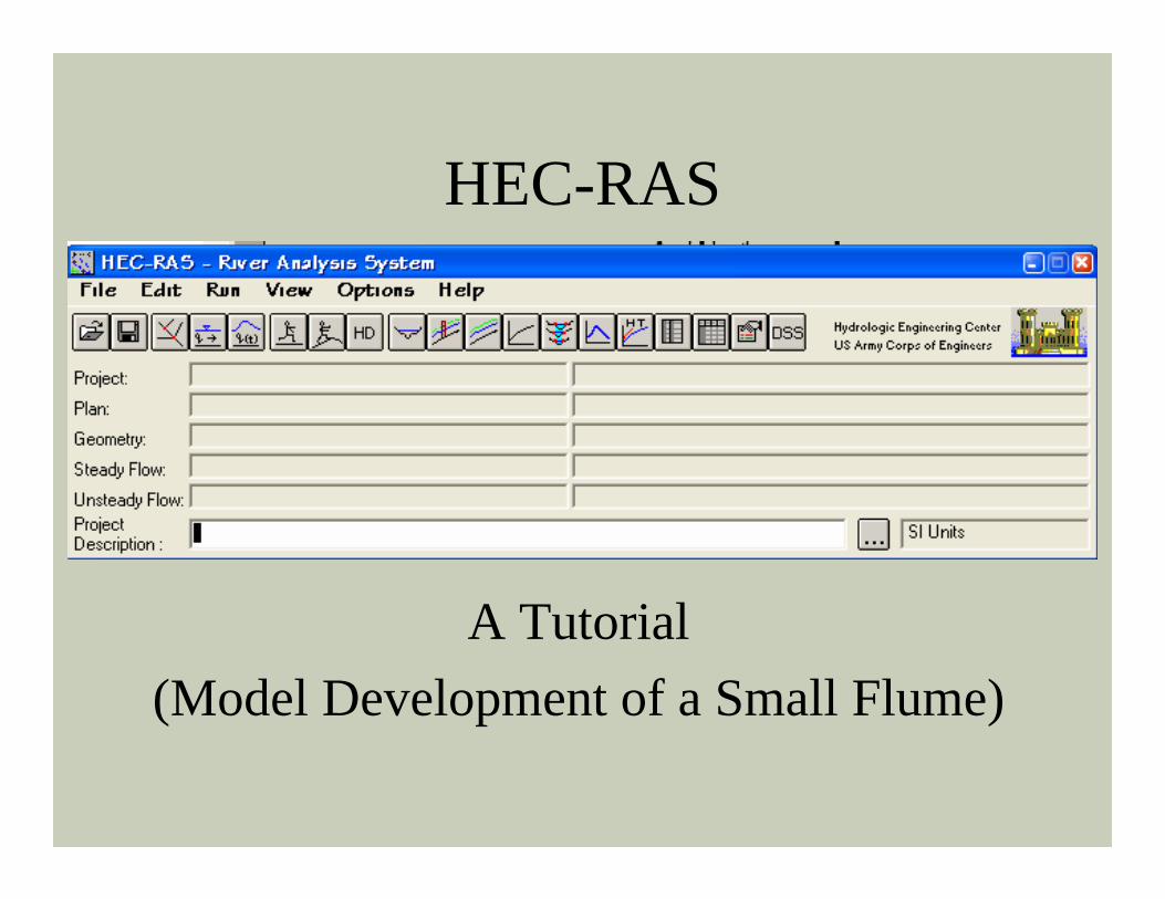
HEC-RAS A Tutorial (Model Development of a Small Flume)
-
Upload
ozren-djuric -
Category
Documents
-
view
48 -
download
0
Transcript of HEC-RAS Tutorial Flume Example
HEC-RAS
A Tutorial(Model Development of a Small Flume)
HEC-RAS
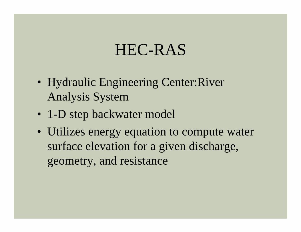
• Hydraulic Engineering Center:River Analysis System
• 1-D step backwater model• Utilizes energy equation to compute water
surface elevation for a given discharge, geometry, and resistance
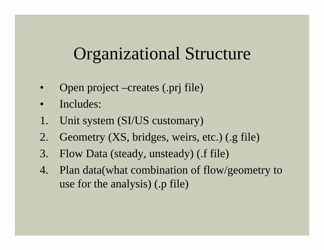
Organizational Structure
• Open project –creates (.prj file)• Includes:1. Unit system (SI/US customary)2. Geometry (XS, bridges, weirs, etc.) (.g file)3. Flow Data (steady, unsteady) (.f file)4. Plan data(what combination of flow/geometry to
use for the analysis) (.p file)
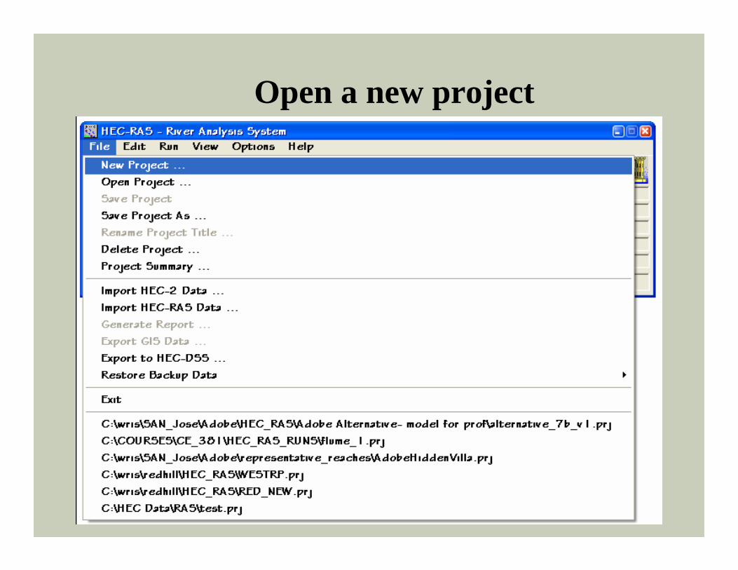
Open a new project
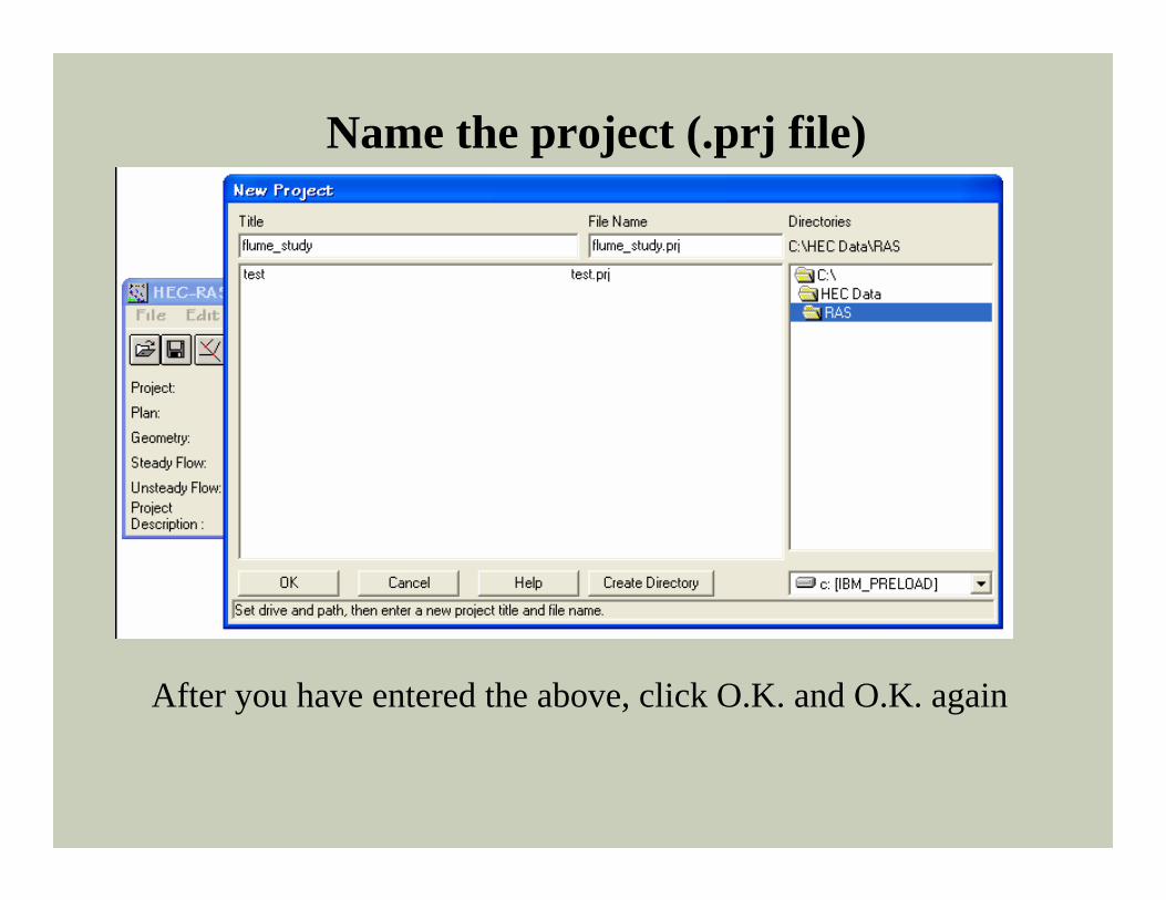
Name the project (.prj file)
After you have entered the above, click O.K. and O.K. again
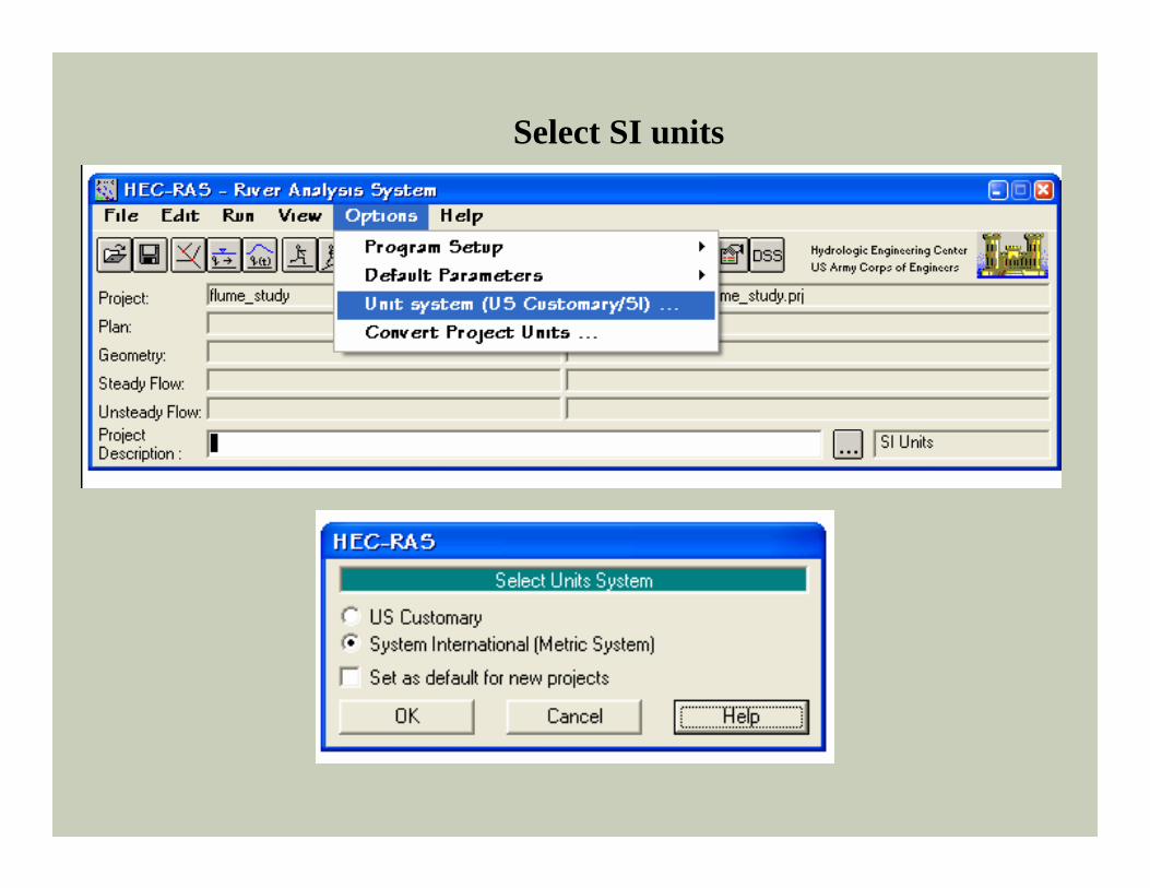
Select SI units
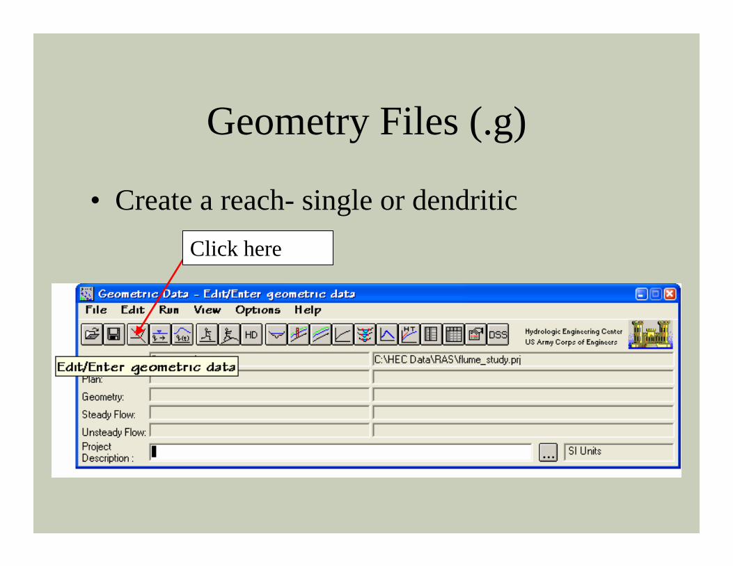
Geometry Files (.g)
• Create a reach- single or dendriticClick here
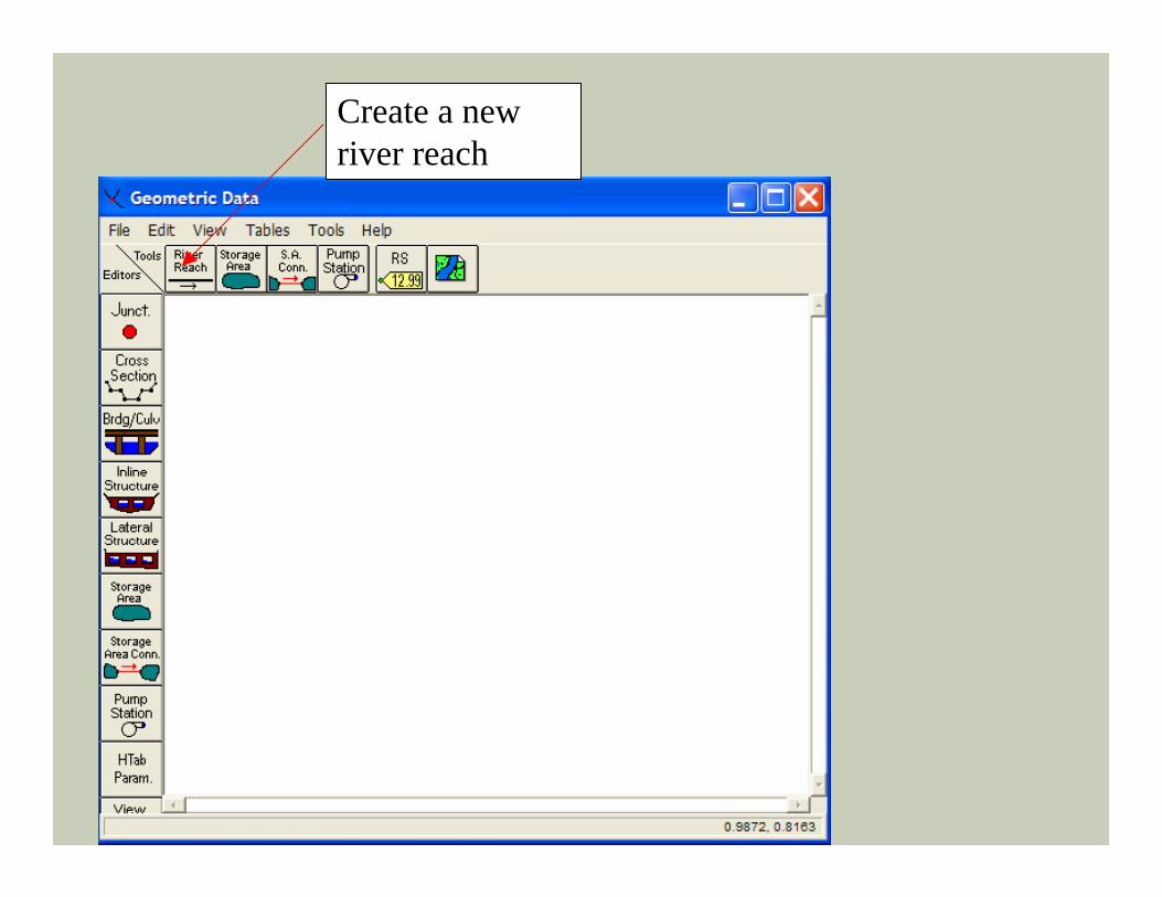
Create a new river reach
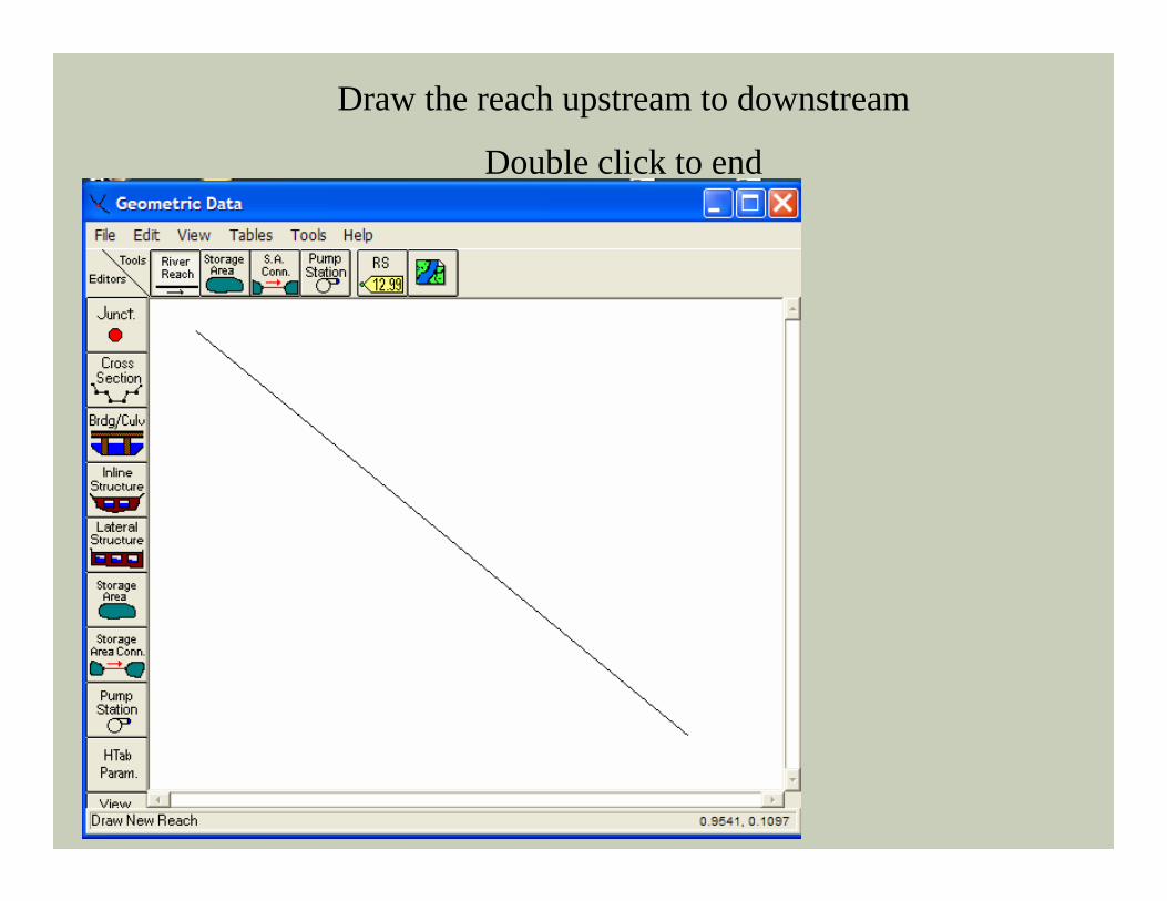
Draw the reach upstream to downstream
Double click to end
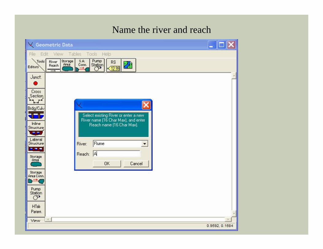
Name the river and reach
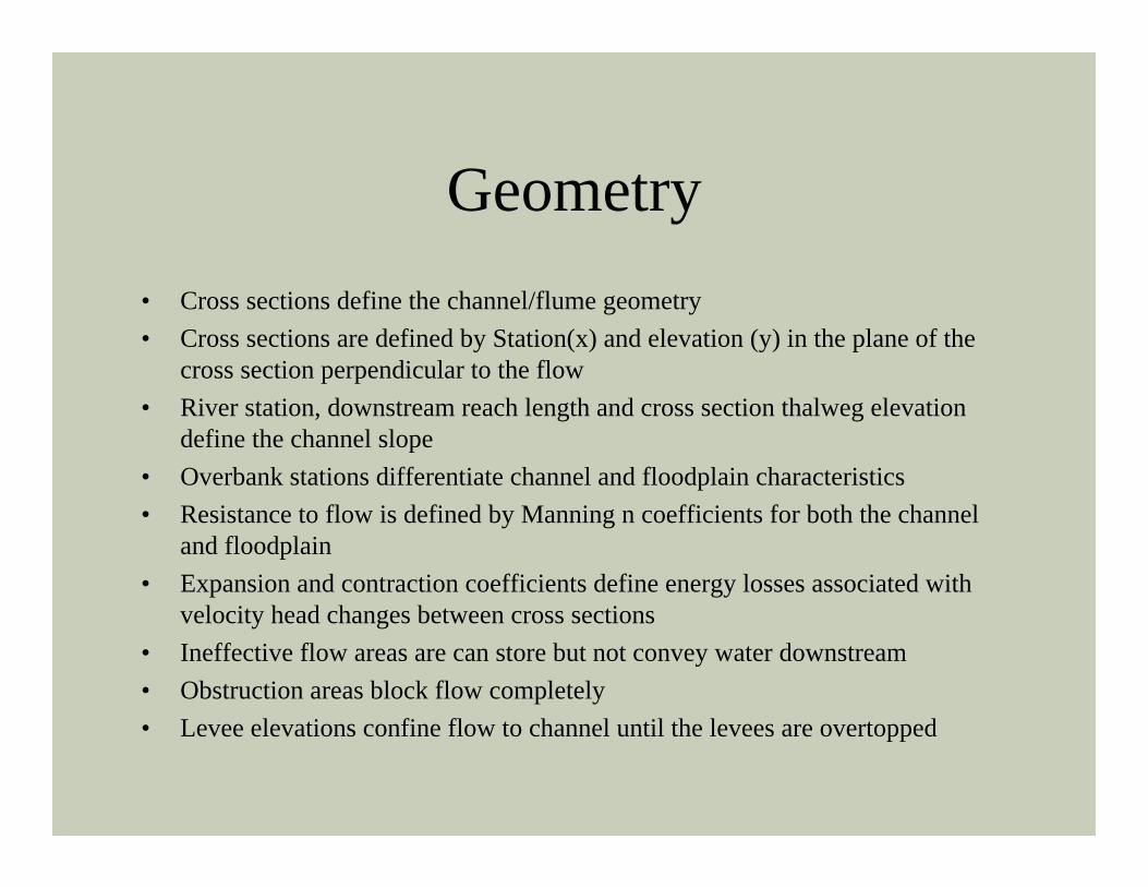
Geometry• Cross sections define the channel/flume geometry• Cross sections are defined by Station(x) and elevation (y) in the plane of the
cross section perpendicular to the flow• River station, downstream reach length and cross section thalweg elevation
define the channel slope• Overbank stations differentiate channel and floodplain characteristics• Resistance to flow is defined by Manning n coefficients for both the channel
and floodplain• Expansion and contraction coefficients define energy losses associated with
velocity head changes between cross sections• Ineffective flow areas are can store but not convey water downstream• Obstruction areas block flow completely• Levee elevations confine flow to channel until the levees are overtopped
More geometry
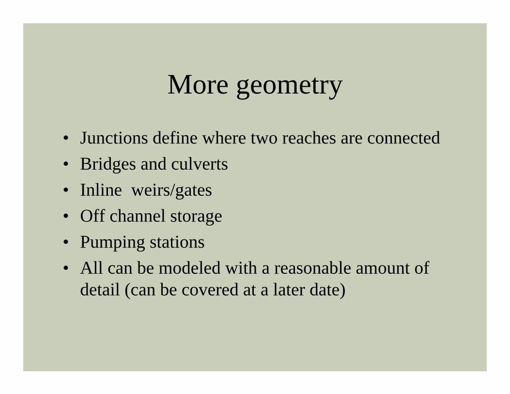
• Junctions define where two reaches are connected• Bridges and culverts• Inline weirs/gates• Off channel storage• Pumping stations• All can be modeled with a reasonable amount of
detail (can be covered at a later date)
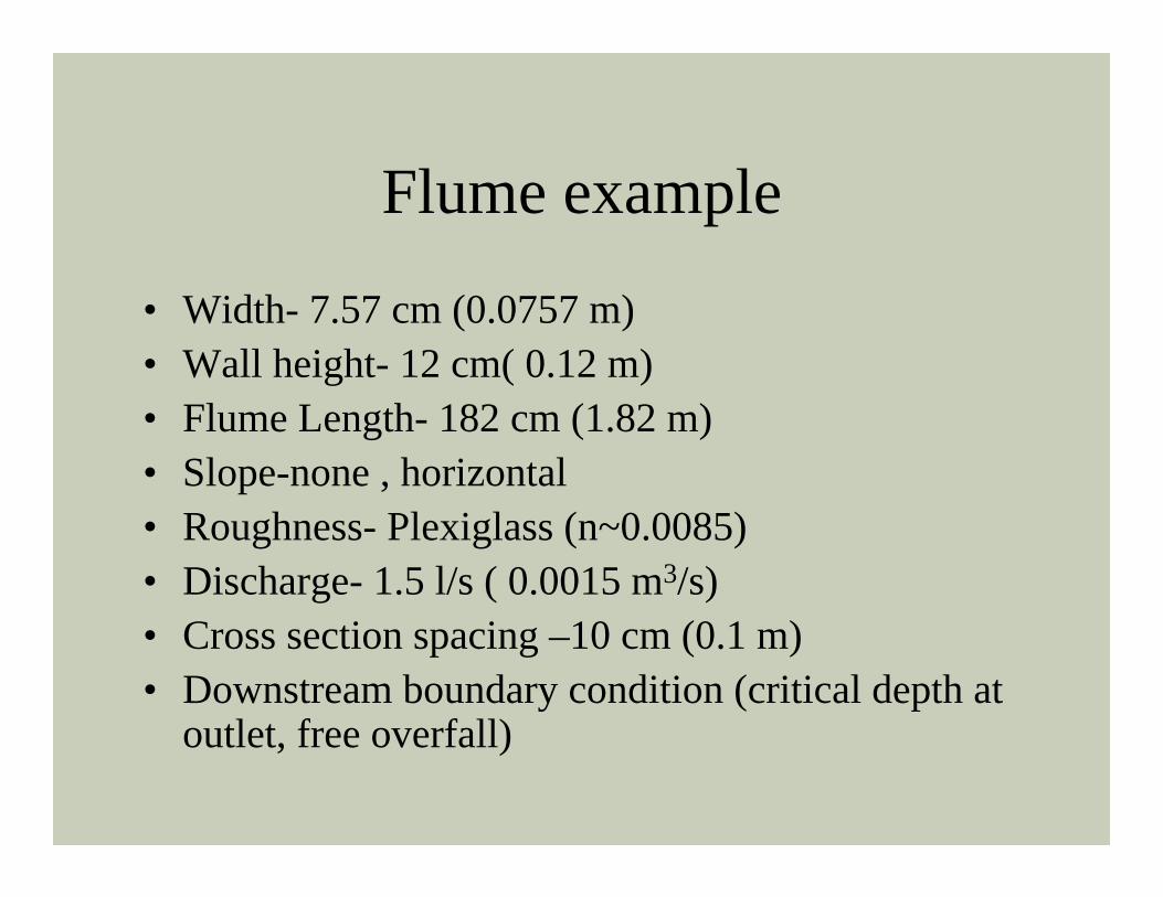
Flume example
• Width- 7.57 cm (0.0757 m)• Wall height- 12 cm( 0.12 m)• Flume Length- 182 cm (1.82 m)• Slope-none , horizontal• Roughness- Plexiglass (n~0.0085)• Discharge- 1.5 l/s ( 0.0015 m3/s)• Cross section spacing –10 cm (0.1 m)• Downstream boundary condition (critical depth at
outlet, free overfall)
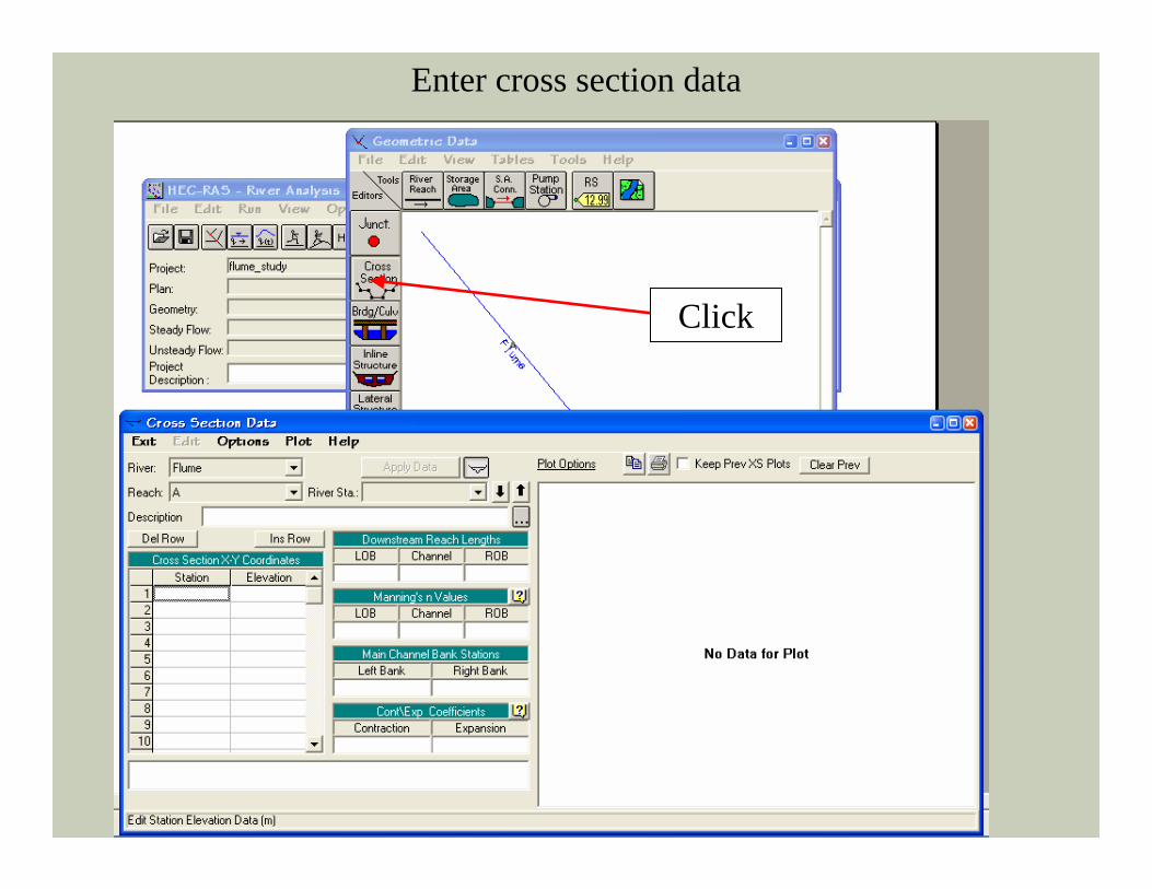
Enter cross section data
Click
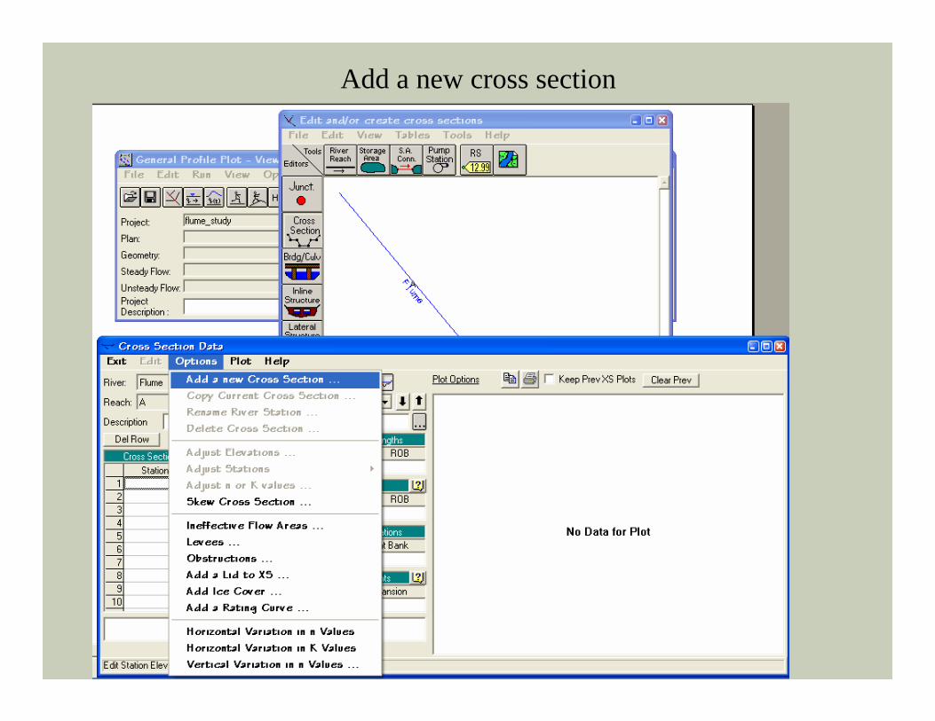
Add a new cross section
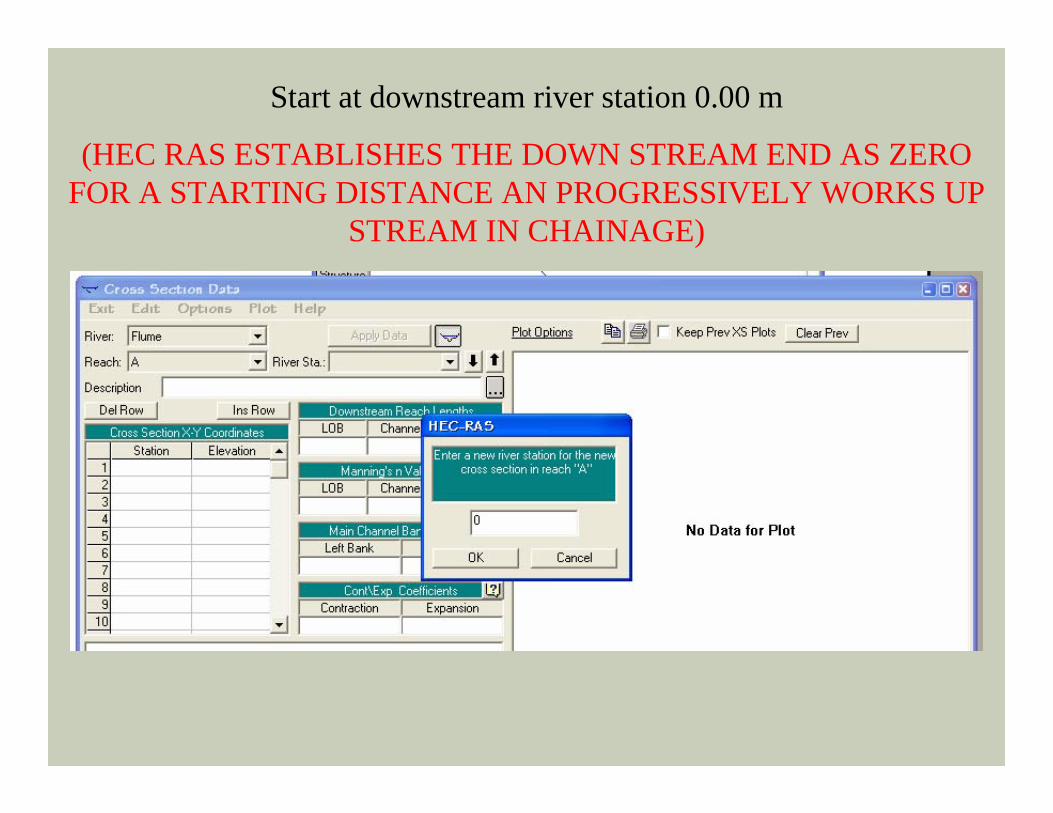
Start at downstream river station 0.00 m
(HEC RAS ESTABLISHES THE DOWN STREAM END AS ZERO FOR A STARTING DISTANCE AN PROGRESSIVELY WORKS UP
STREAM IN CHAINAGE)
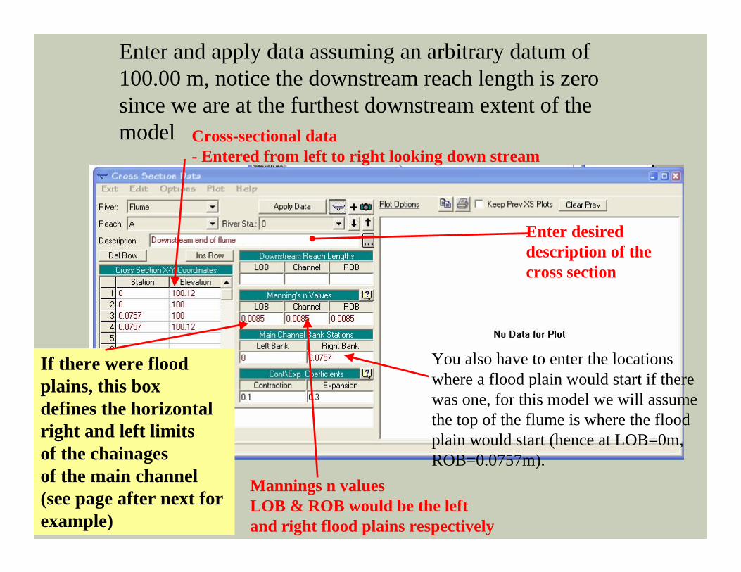
Enter and apply data assuming an arbitrary datum of 100.00 m, notice the downstream reach length is zero since we are at the furthest downstream extent of the model Cross-sectional data
- Entered from left to right looking down stream
Mannings n valuesLOB & ROB would be the left and right flood plains respectively
If there were floodplains, this boxdefines the horizontalright and left limitsof the chainagesof the main channel(see page after next for example)
Enter desired description of the cross section
You also have to enter the locations where a flood plain would start if there was one, for this model we will assume the top of the flume is where the flood plain would start (hence at LOB=0m, ROB=0.0757m).
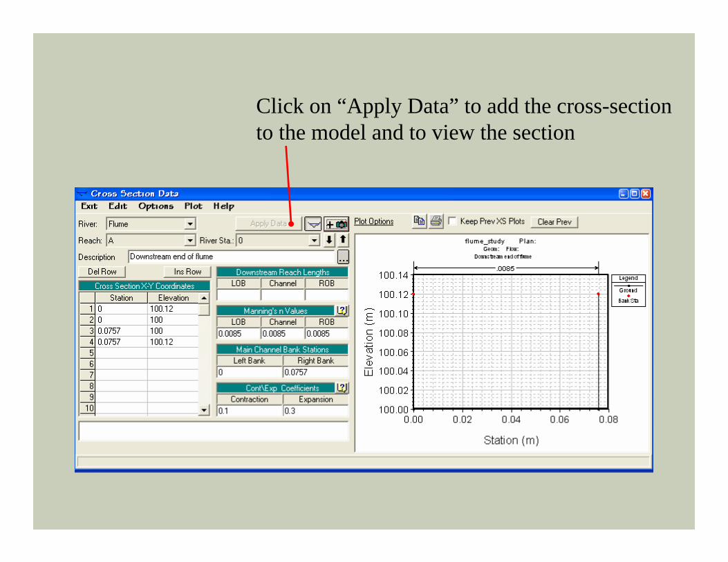
Click on “Apply Data” to add the cross-sectionto the model and to view the section

Main Channel Chainage Definition
Flume Example Note the differentManning’s nvalues in the channeland on the right andleft flood plains for a river.
AdobeCreekExample
Since the geometry is uniform from the upstream to downstream extent, we can make use of the cross section interpolation tool to compute the geometry with the specified cross section spacing
This will take
a few steps….

Add a new cross section at the upstream end river station 1.82 m
(Since we have the same geometry we are going to make use of thecopy section function)
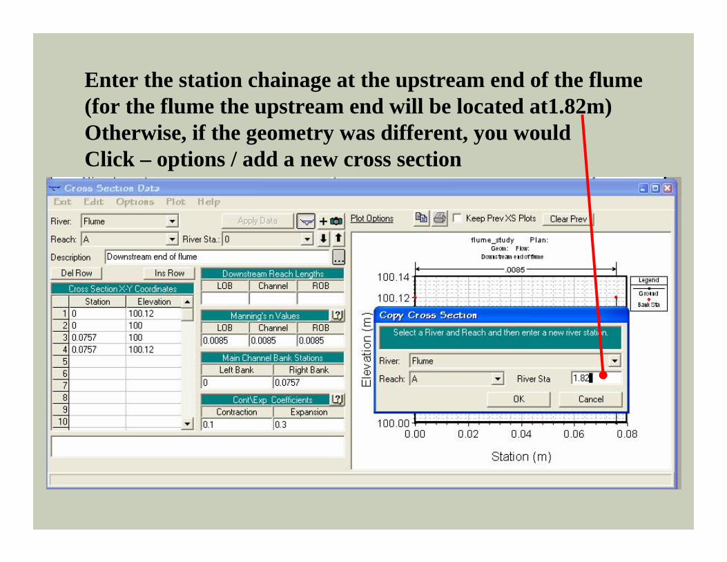
Enter the station chainage at the upstream end of the flume(for the flume the upstream end will be located at1.82m)Otherwise, if the geometry was different, you wouldClick – options / add a new cross section
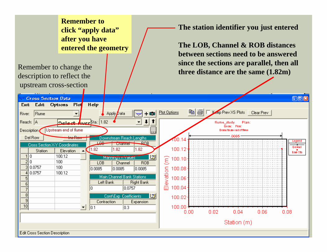
The station identifier you just entered
The LOB, Channel & ROB distancesbetween sections need to be answeredsince the sections are parallel, then all three distance are the same (1.82m)
Remember toclick “apply data”after you haveentered the geometry
Remember to change thedescription to reflect theupstream cross-section
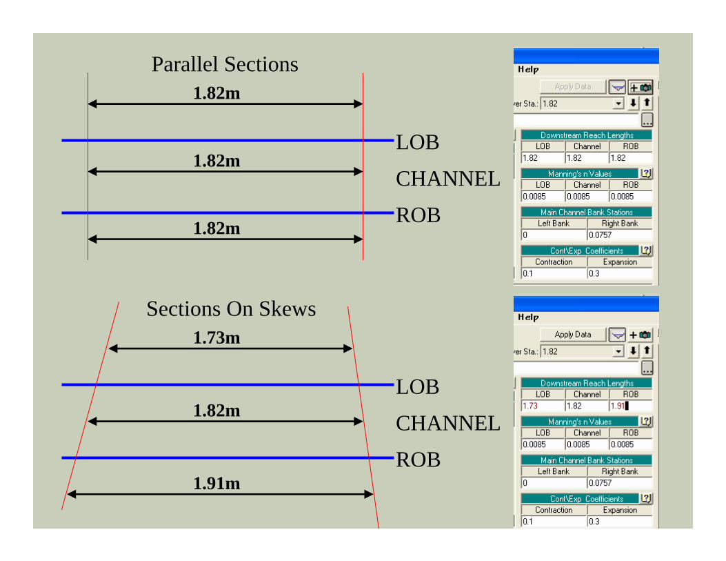
LOB
ROB
CHANNEL
Parallel Sections
Sections On Skews
1.82m
1.91m
1.82m
1.73m
1.82m
1.82m
LOB
ROB
CHANNEL
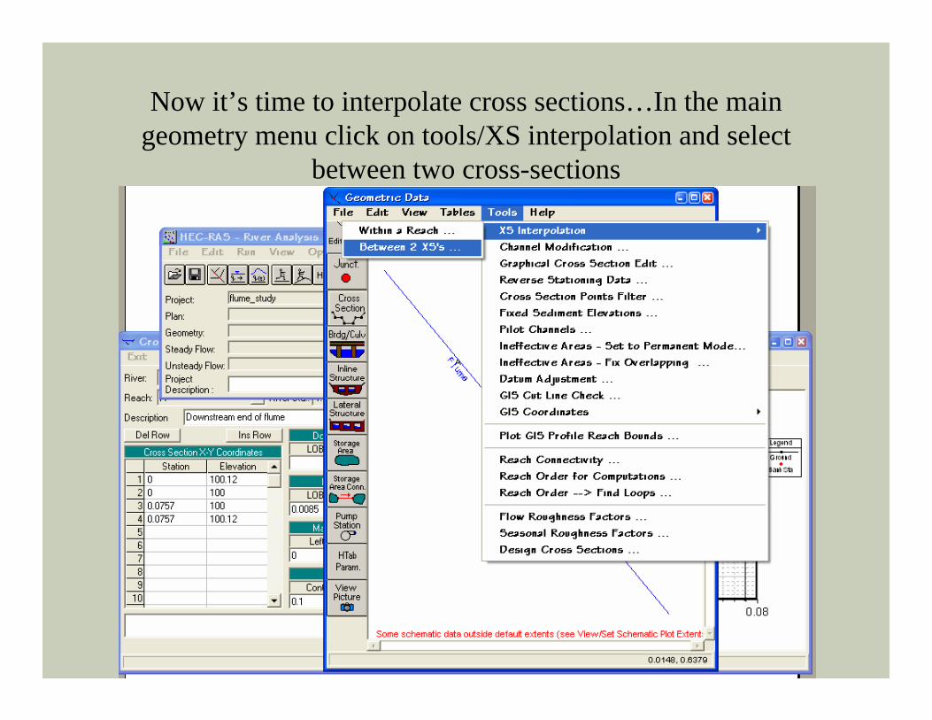
Now it’s time to interpolate cross sections…In the main geometry menu click on tools/XS interpolation and select
between two cross-sections
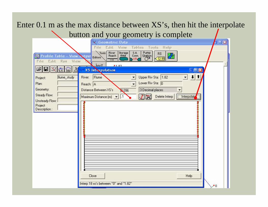
Enter 0.1 m as the max distance between XS’s, then hit the interpolate button and your geometry is complete
If you continued to have different cross sectional geometry at each cross-section, you would continue to add new cross-
sections and enter the distances between each section.
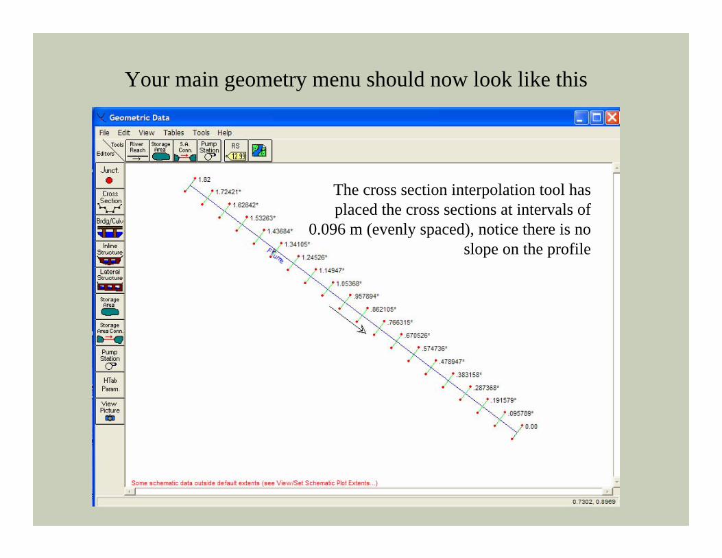
Your main geometry menu should now look like this
The cross section interpolation tool has placed the cross sections at intervals of
0.096 m (evenly spaced), notice there is no slope on the profile
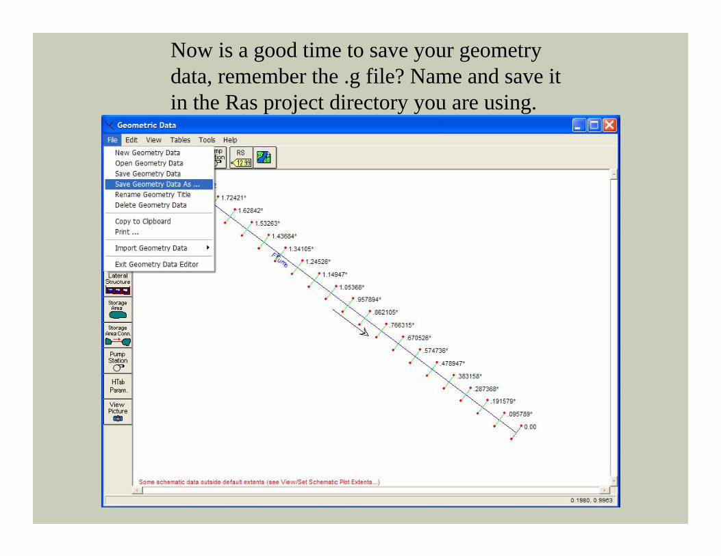
Now is a good time to save your geometry data, remember the .g file? Name and save it in the Ras project directory you are using.
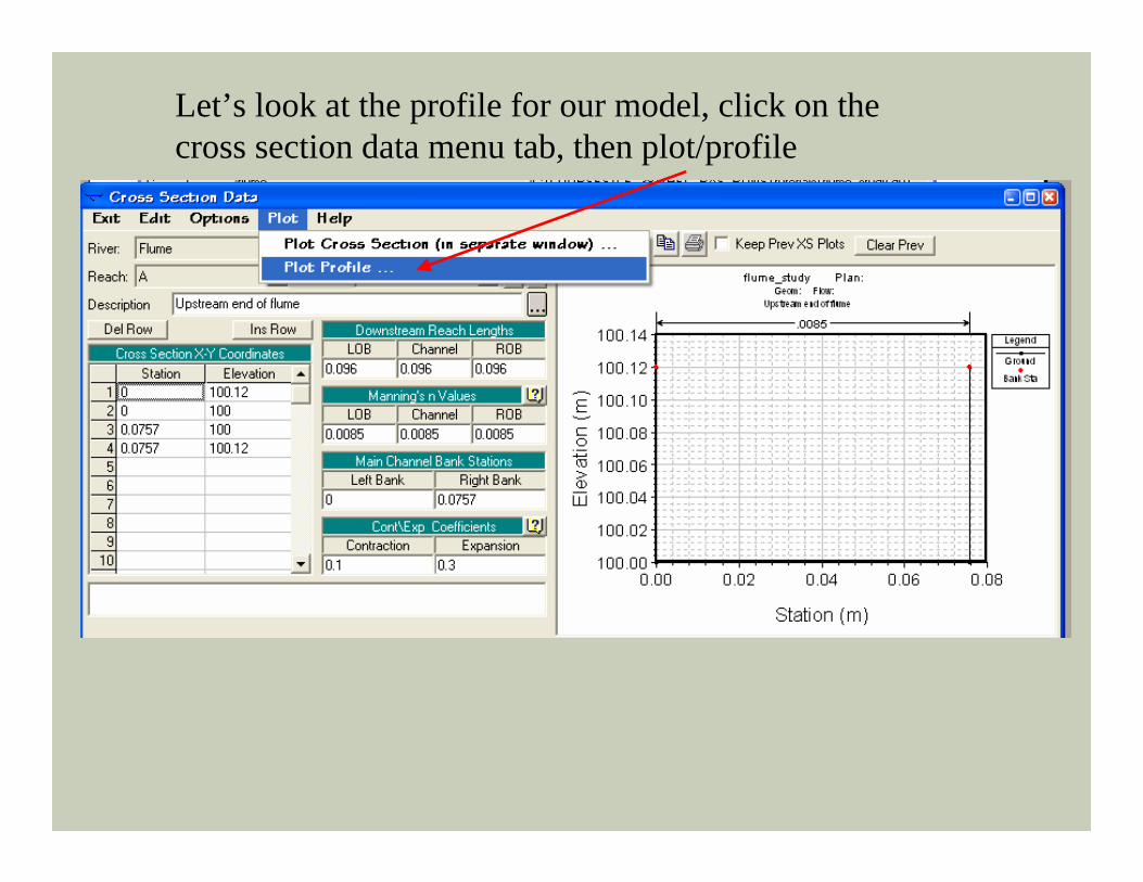
Let’s look at the profile for our model, click on the cross section data menu tab, then plot/profile
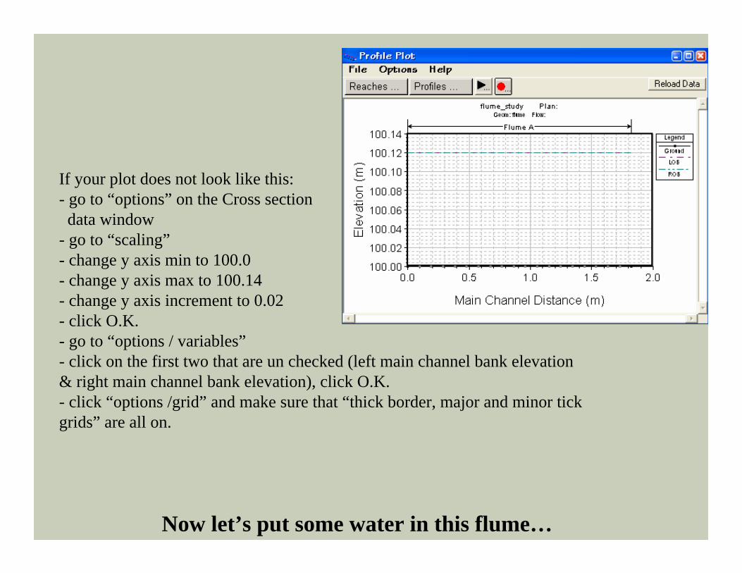
Now let’s put some water in this flume…
If your plot does not look like this:- go to “options” on the Cross section data window
- go to “scaling”- change y axis min to 100.0- change y axis max to 100.14- change y axis increment to 0.02- click O.K.- go to “options / variables”- click on the first two that are un checked (left main channel bank elevation & right main channel bank elevation), click O.K.- click “options /grid” and make sure that “thick border, major and minor tick grids” are all on.
Flow data (.f files)
• Steady (constant with time)• Unsteady (varies with time)• Regimes( supercritical, subcritical, mixed)• Boundary conditions:
1. Supercritical-upstream2. Subcritical-downstream3. Mixed-both
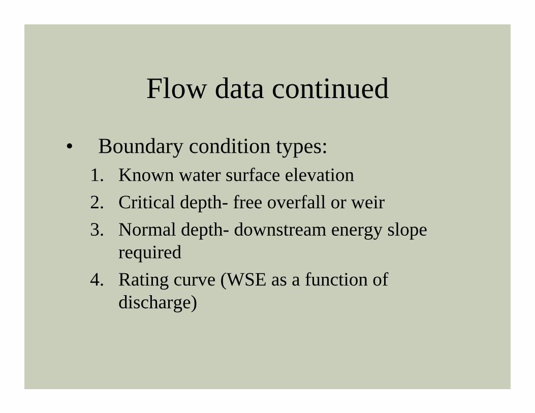
Flow data continued
• Boundary condition types:1. Known water surface elevation2. Critical depth- free overfall or weir3. Normal depth- downstream energy slope
required4. Rating curve (WSE as a function of
discharge)
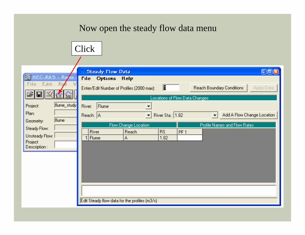
Click
Now open the steady flow data menu
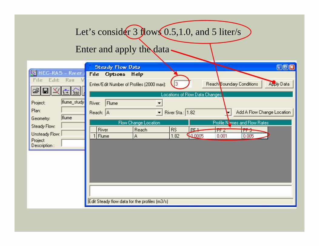
Let’s consider 3 flows 0.5,1.0, and 5 liter/s
Enter and apply the data
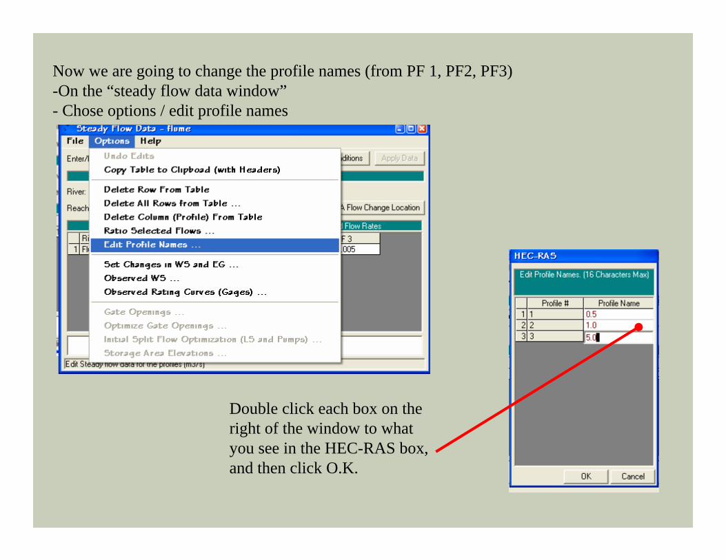
Now we are going to change the profile names (from PF 1, PF2, PF3)-On the “steady flow data window”- Chose options / edit profile names
Double click each box on the right of the window to what you see in the HEC-RAS box, and then click O.K.
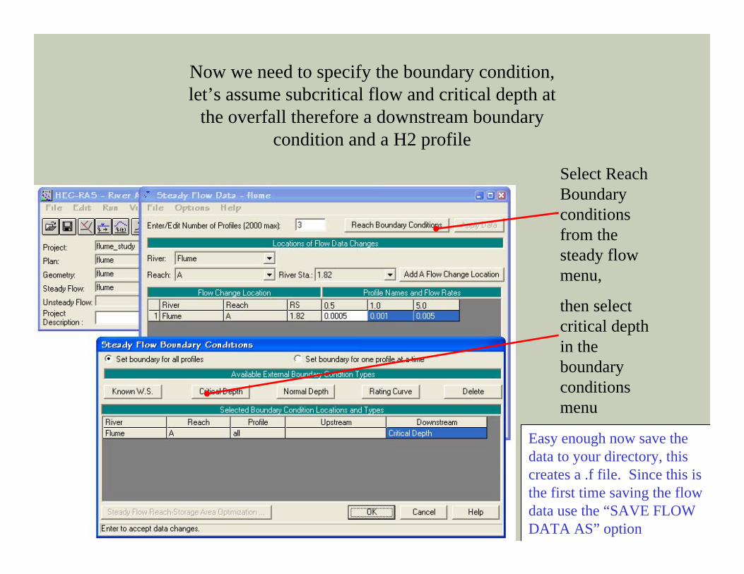
Now we need to specify the boundary condition, let’s assume subcritical flow and critical depth at
the overfall therefore a downstream boundary condition and a H2 profile
Select Reach Boundary conditions from the steady flow menu,
then select critical depth in the boundary conditions menu
Easy enough now save the data to your directory, this creates a .f file. Since this is the first time saving the flow data use the “SAVE FLOW DATA AS” option
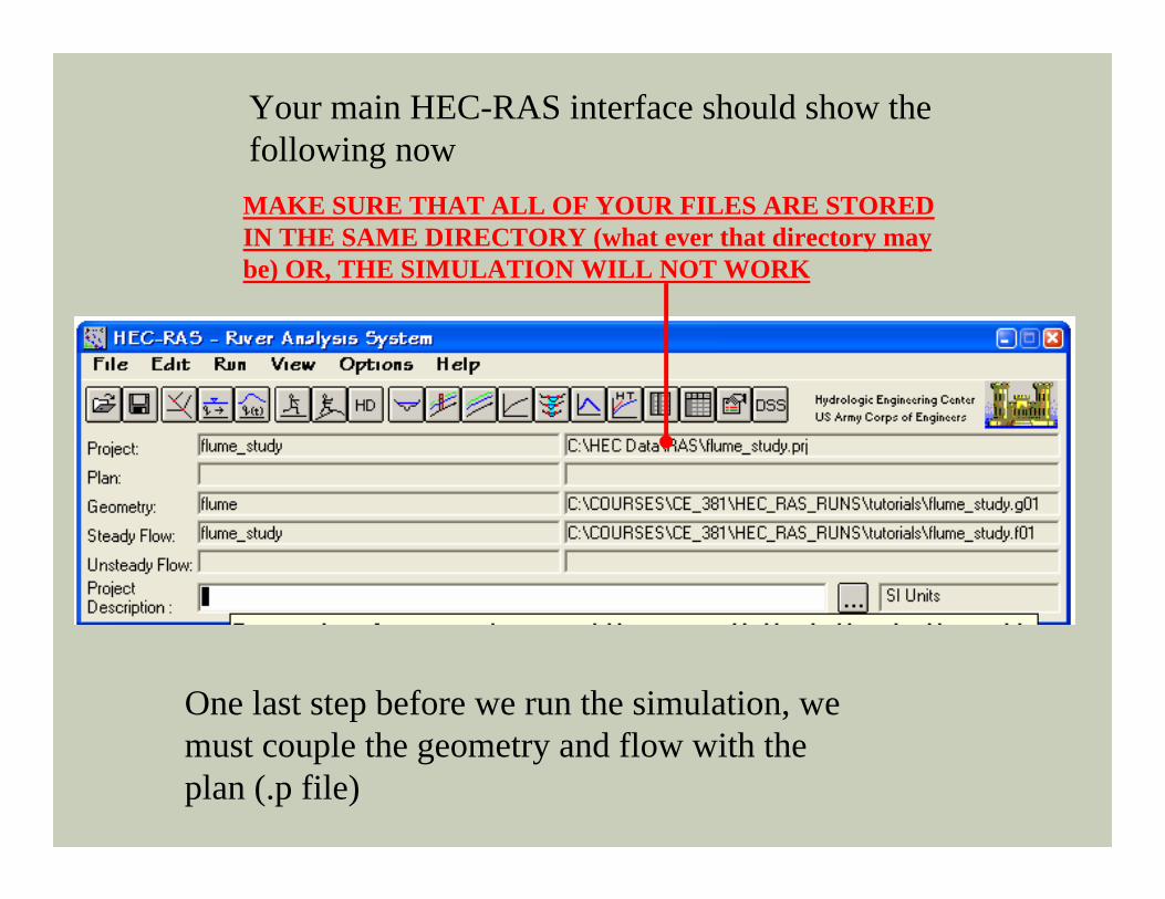
Your main HEC-RAS interface should show the following now
One last step before we run the simulation, we must couple the geometry and flow with the plan (.p file)
MAKE SURE THAT ALL OF YOUR FILES ARE STORED IN THE SAME DIRECTORY (what ever that directory may be) OR, THE SIMULATION WILL NOT WORK
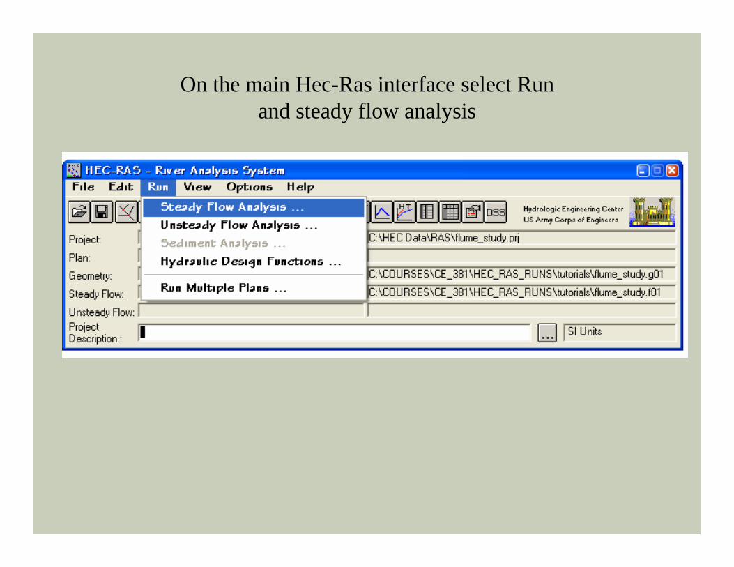
On the main Hec-Ras interface select Run and steady flow analysis
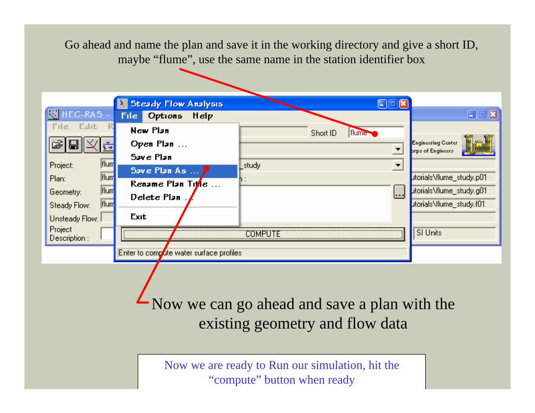
Now we can go ahead and save a plan with the existing geometry and flow data
Go ahead and name the plan and save it in the working directory and give a short ID, maybe “flume”, use the same name in the station identifier box
Now we are ready to Run our simulation, hit the “compute” button when ready
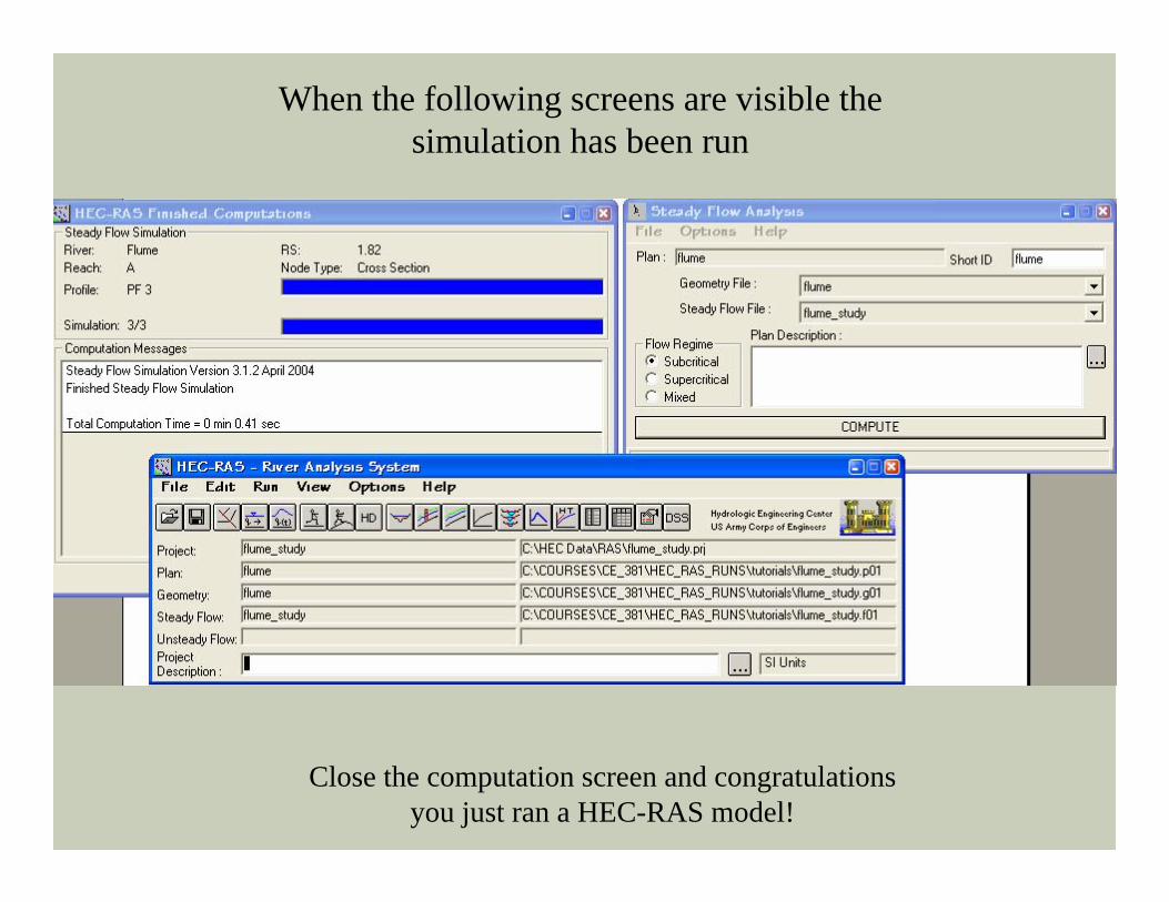
When the following screens are visible the simulation has been run
Close the computation screen and congratulations you just ran a HEC-RAS model!
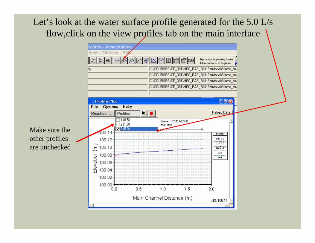
Let’s look at the water surface profile generated for the 5.0 L/s flow,click on the view profiles tab on the main interface
Make sure theother profilesare unchecked

A series of variables can be plotted on the profile.Lets add the critical flow depth….Navigate to options / variables on the Profile Plot Window
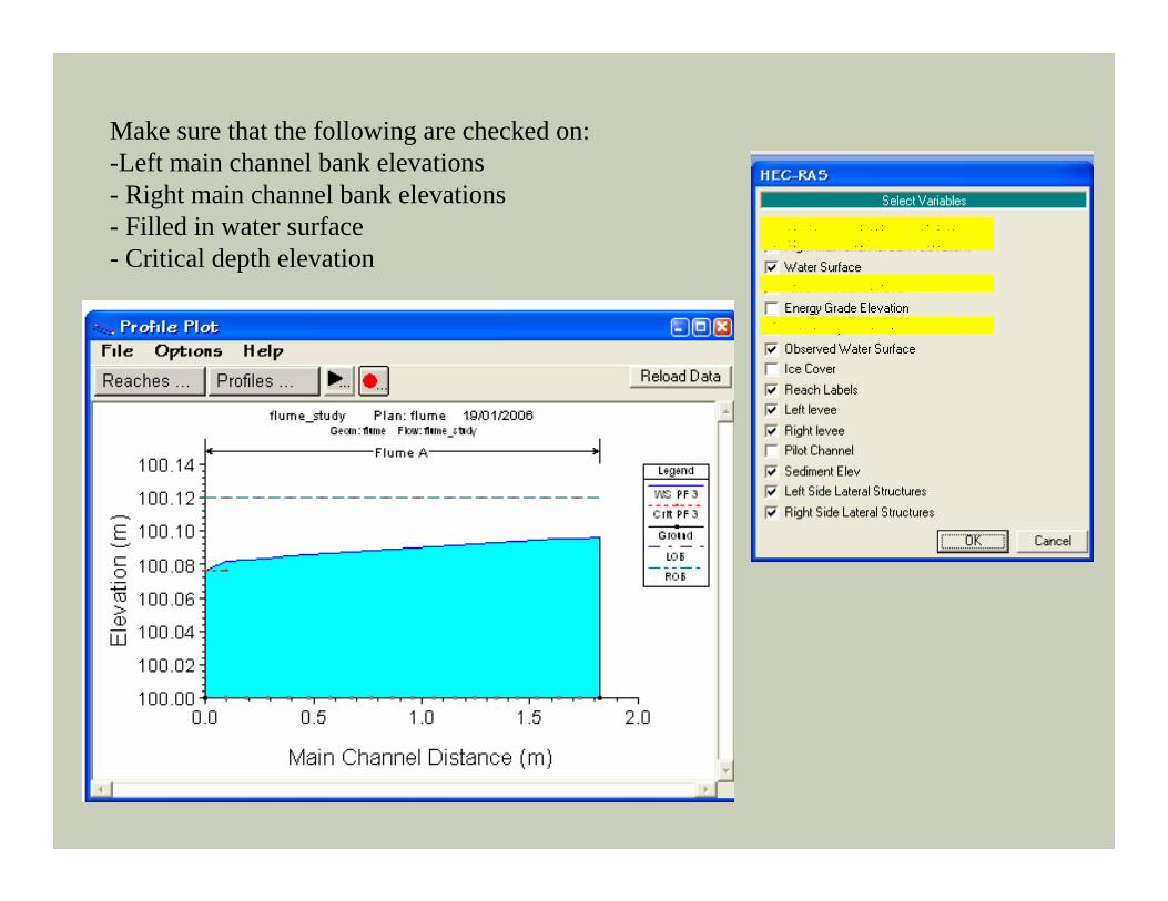
Make sure that the following are checked on:-Left main channel bank elevations- Right main channel bank elevations- Filled in water surface- Critical depth elevation
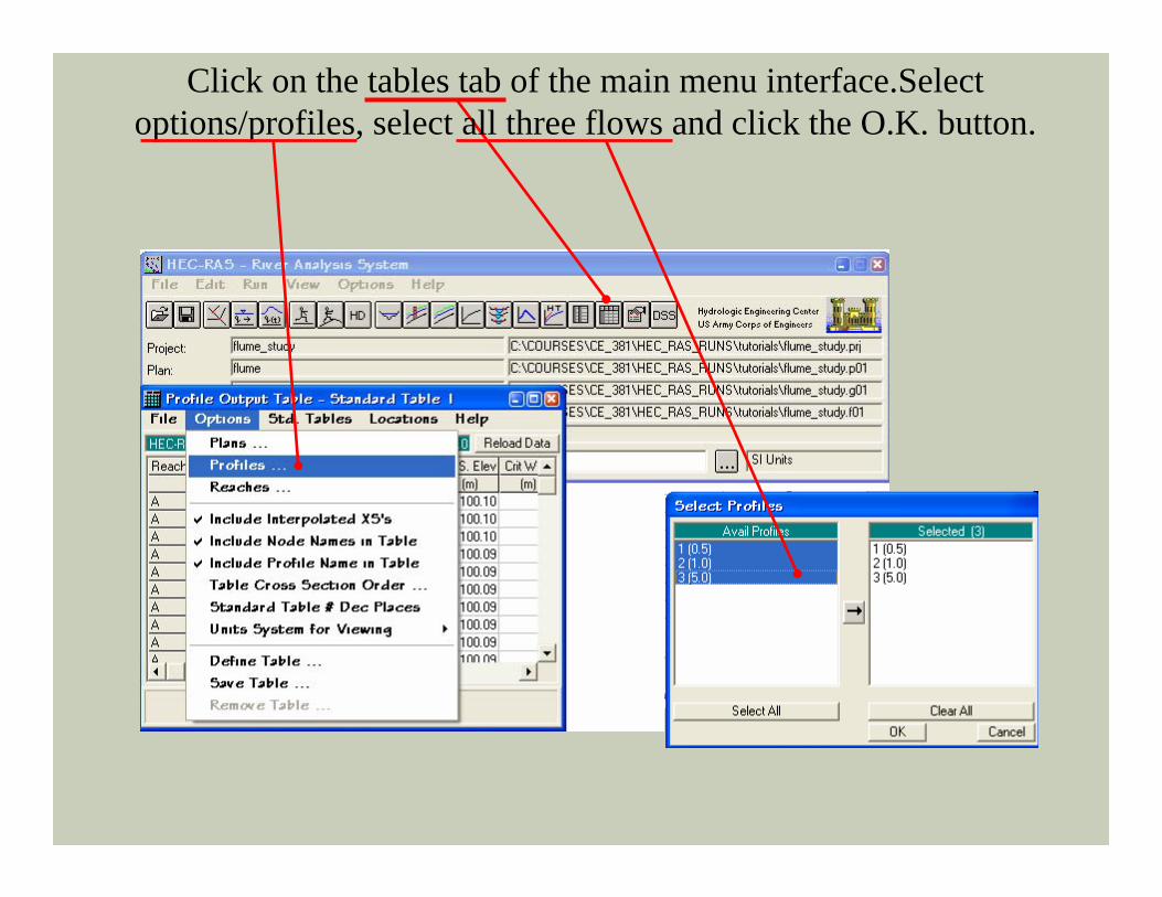
Click on the tables tab of the main menu interface.Select options/profiles, select all three flows and click the O.K. button.
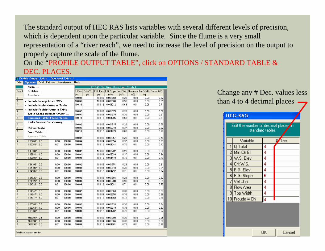
The standard output of HEC RAS lists variables with several different levels of precision, which is dependent upon the particular variable. Since the flume is a very small representation of a “river reach”, we need to increase the level of precision on the output to properly capture the scale of the flume.On the “PROFILE OUTPUT TABLE”, click on OPTIONS / STANDARD TABLE & DEC. PLACES.
Change any # Dec. values less than 4 to 4 decimal places
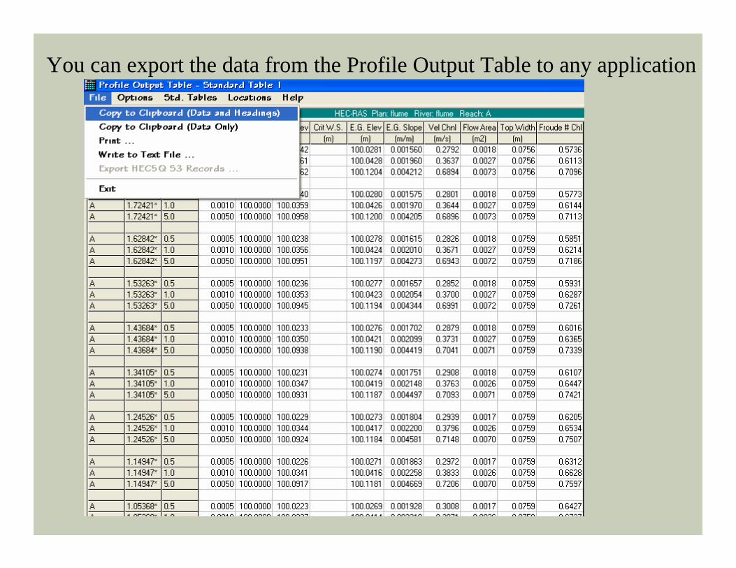
You can export the data from the Profile Output Table to any application
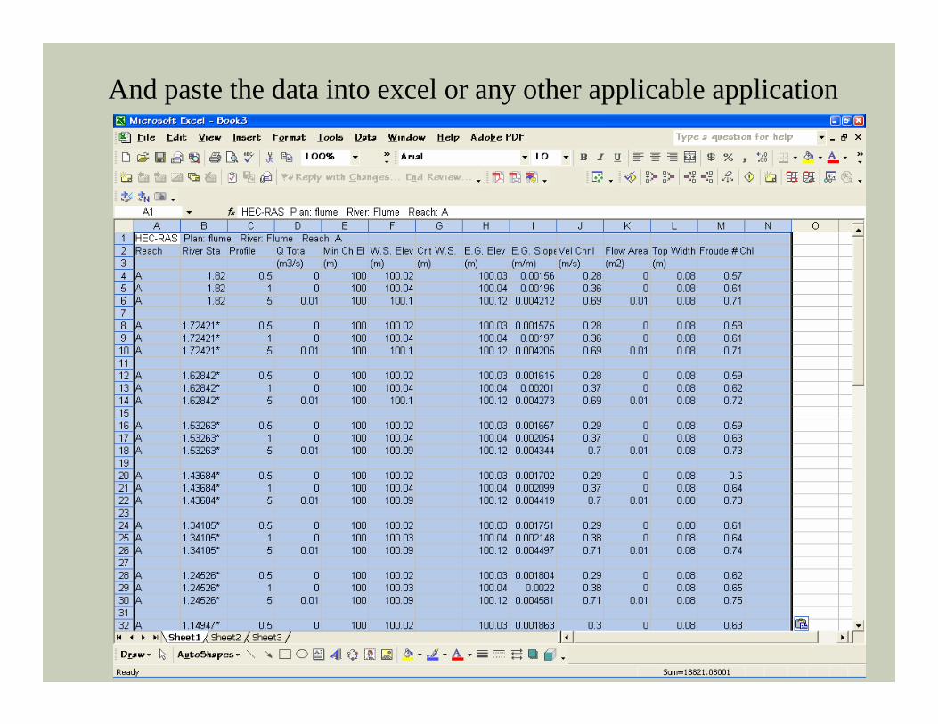
And paste the data into excel or any other applicable application
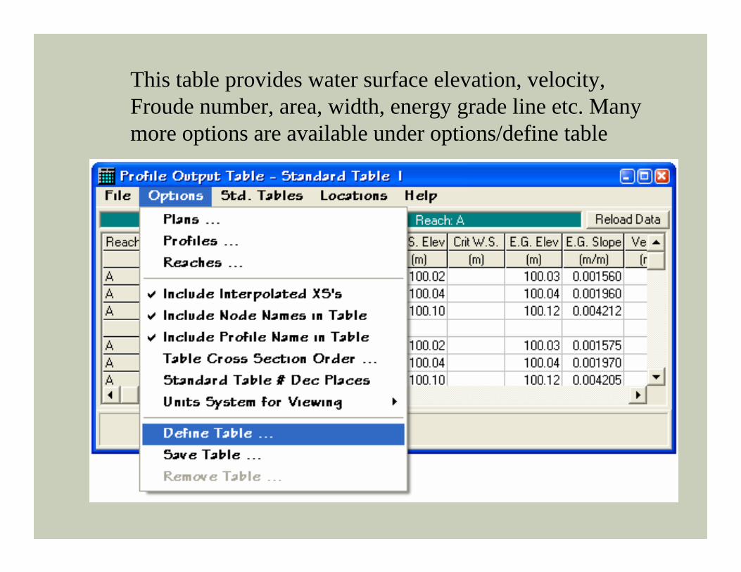
This table provides water surface elevation, velocity, Froude number, area, width, energy grade line etc. Many more options are available under options/define table
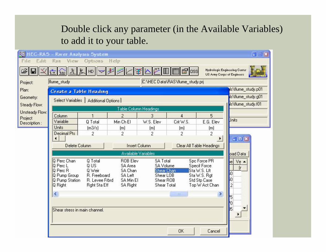
Double click any parameter (in the Available Variables)to add it to your table.
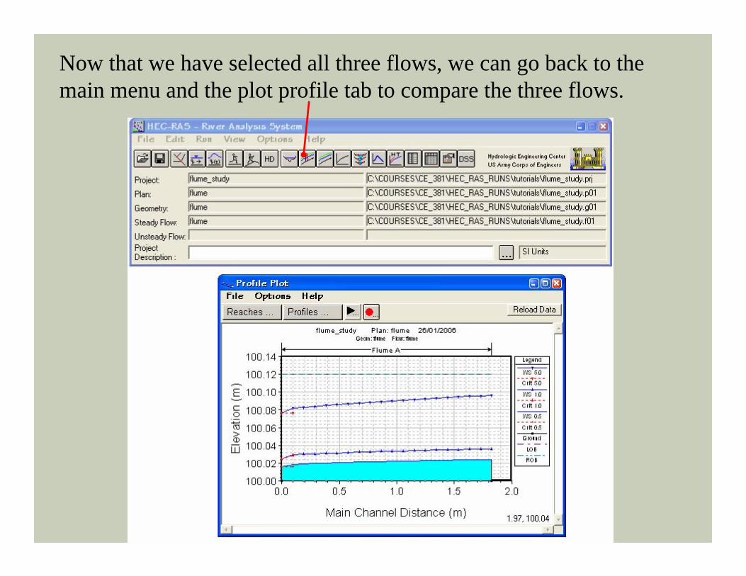
Now that we have selected all three flows, we can go back to themain menu and the plot profile tab to compare the three flows.
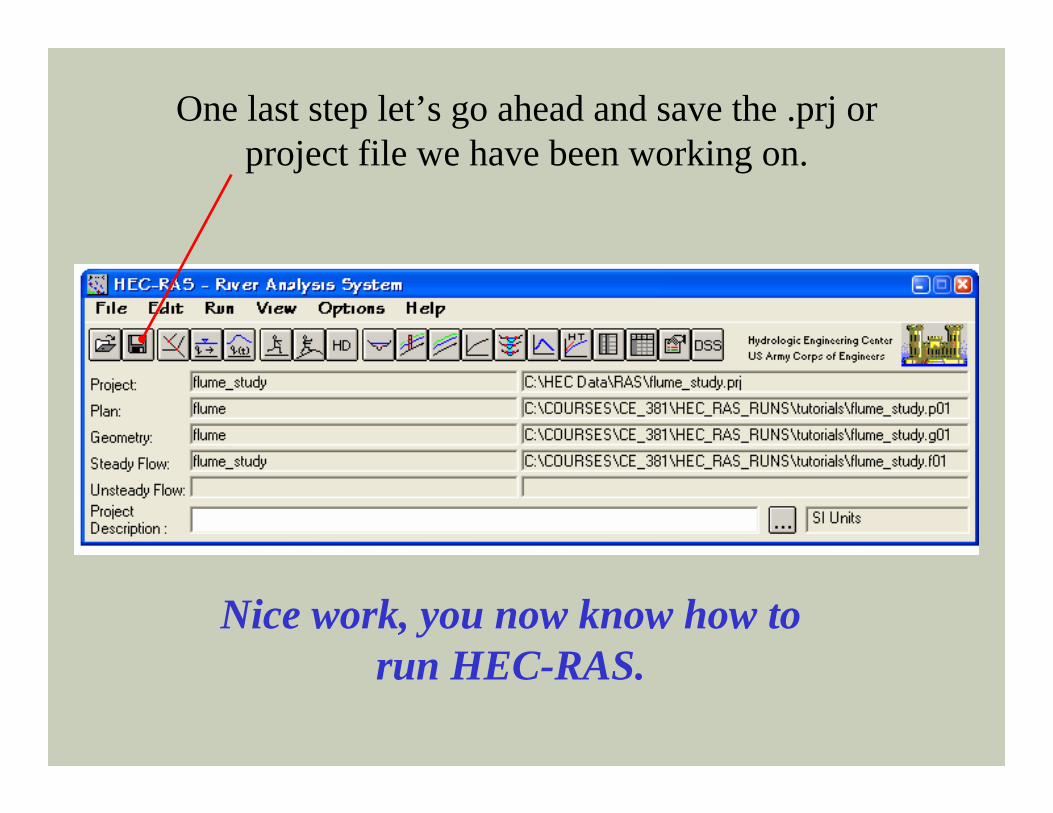
One last step let’s go ahead and save the .prj or project file we have been working on.
Nice work, you now know how to run HEC-RAS.
0 0.1 0.2 0.3 0.4 0.5 0.6 0.7 0.8 0.9 1 1.1 1.2 1.3 1.4 1.5 1.6 1.7 1.8
CHAINAGE (m)
100.00
100.01
100.02
100.03
100.04
100.05
100.06
100.07
100.08
100.09
100.10
100.11
100.12
Rel
eativ
e El
evat
ion
(m)
HEC RAS Model (Best fit)OBSERVED DATA
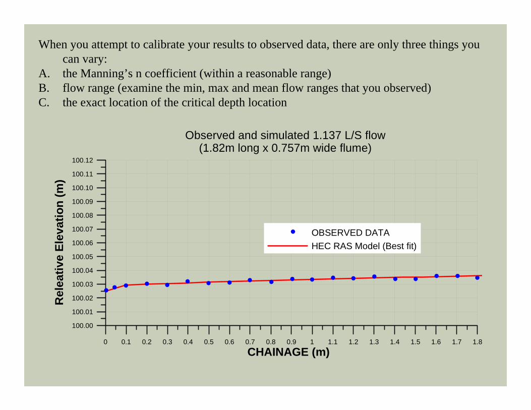
Observed and simulated 1.137 L/S flow(1.82m long x 0.757m wide flume)
When you attempt to calibrate your results to observed data, there are only three things you can vary:
A. the Manning’s n coefficient (within a reasonable range)B. flow range (examine the min, max and mean flow ranges that you observed)C. the exact location of the critical depth location