Heat and Mass Transfer - sv.20file.orgsv.20file.org/up1/419_0.pdf · analysis method to replace the...
368
Transcript of Heat and Mass Transfer - sv.20file.orgsv.20file.org/up1/419_0.pdf · analysis method to replace the...
Heat and Mass Transfer
Series Editors: D. Mewes and F. Mayinger
For further volumes:http://www.springer.com/series/4247

Deyi Shang
Theory of Heat Transferwith Forced ConvectionFilm Flows
With 62 Figures
123
Prof. Dr. Deyi Shang9 Westmeath Cr.Ottawa, ON, CanadaK2K [email protected]
ISSN 1860-4846 e-ISSN 1860-4854ISBN 978-3-642-12580-5 e-ISBN 978-3-642-12581-2DOI 10.1007/978-3-642-12581-2Springer Heidelberg Dordrecht London New York
Library of Congress Control Number: 2010933612
c© Springer-Verlag Berlin Heidelberg 2011This work is subject to copyright. All rights are reserved, whether the whole or part of the materialis concerned, specifically the rights of translation, reprinting, reuse of illustrations, recitation,broadcasting, reproduction on microfilm or in any other way, and storage in data banks. Duplicationof this publication or parts thereof is permitted only under the provisions of the German CopyrightLaw of September 9, 1965, in its current version, and permission for use must always be obtained fromSpringer. Violations are liable to prosecution under the German Copyright Law.The use of general descriptive names, registered names, trademarks, etc. in this publication does notimply, even in the absence of a specific statement, that such names are exempt from the relevantprotective laws and regulations and therefore free for general use.
Cover design: deblik, Berlin
Printed on acid-free paper
Springer is part of Springer Science+Business Media (www.springer.com)

Preface
This book presents recent developments in my research on heat transfer of laminarforced convection and its film condensation. It is a monograph on advanced heattransfer, provided for university postgraduate students as textbook, students in self-study, researchers and professors as an academic reference book, and engineers anddesigners as a scientific handbook. A primary goal is to present a new similarityanalysis method to replace the traditional Falkner-Skan type transformation for adeep investigation in this book. This method is so important that it becomes a theo-retical basis of this book. A secondary goal is to report a system of research devel-opments for heat and mass transfer of laminar forced convection and its two-phasefilm condensation, based on the present new similarity analysis method.
The book includes three parts: (1) theoretical foundation, including presenta-tion of basic conservation equations for laminar convection, review of Falkner-Skan transformation for laminar forced convection boundary layer, and creationof the new similarity analysis method related to laminar forced convection and itstwo-phase film condensation; (2) laminar forced convection, including a systemof complete similarity mathematical models based on the new similarity analysismethod, rigorous numerical results of velocity and temperature fields, and advancedresearch results on heat transfer with ignoring variable physical properties or viscousthermal dissipation, considering viscous thermal dissipation, and considering cou-pled effect of variable physical properties; and (3) laminar forced film condensation,including a system of complete similarity mathematical models based on the newsimilarity analysis method, rigorous numerical results of velocity, temperature, andconcentration fields, and advanced research achievements on condensate heat andmass transfer. In the research of this book, the following difficult issues have beenresolved. They are (i) creating the new similarity analysis method, (ii) developingthe system of complete similarity mathematical models, (iii) rigorously dealing withthe variable physical properties, (iv) obtaining the reliable numerical results withsatisfying whole interfacial physical matching conditions for the forced convectionfilm condensation, (v) clarifying the effect of noncondensable gas on interfacialvapour saturation temperature as well as heat and mass transfer of the film con-densation of vapour–gas mixture, (vi) clarifying the coupled effects of temperature-dependent physical properties on heat transfer of laminar forced convection, (vii)clarifying the coupled effect of concentration and temperature- dependent physical
v

vi Preface
properties on heat and mass transfer of forced convection film condensation, (viii)creating a series of reliable prediction equations on heat and mass transfer for prac-tical application, etc. Having resolved all above difficult issues demonstrates thescientific contributions of this book to extensive research on heat and mass transferof laminar forced convection and its film condensation.
Obviously, all above difficult issues resolved in this book are big challengesencountered in my recent research. While the most significant challenge is howto clarify heat and mass transfer and create the related reliable prediction equationswith consideration of various complicated physical factors including the coupledeffect of variable physical properties, in order to realize theoretically reliable andconvenient prediction of heat and mass transfer. For this purpose, all related variablephysical properties are based on the experimental data, and rigorously dealt with inthe complete similarity mathematical models in the system of related investigationsof this book. On this basis, the theoretical research results of this book have theirreliable application values.
In this book, all flows are taken on a horizontal flat plate for a research system-ization. However, the present new similarity analysis method is suitable for generaltype of laminar forced convection and its film condensation. The research of thisbook has a spread space.
Here, I am very sincerely grateful to Professor Liangcai Zhong, NortheasternUniversity, China, who provided his great help for development of the related math-ematical models and numerical calculation. This book involves his significant con-tribution. I am heartily thankful to Professor B.X. Wang, my supervisor of my Ph.Dr.study from 1988 to 1991 in Tsinghua University, China, whose profound knowledgeof the speciality, strict style of investigation, encouragement, and support enabledme to develop the challenging research. My respective friend, Mr. Sam Gelman gaveup his holiday during the period of New Year going through parts of the manuscript.I would like to offer my sincere gratitude to him for all his help, support, hints, andvaluable improvements.
I am so thankful for my wife Shihua Sun’s sustained moral encouragements,which gave me a long-term power to persist in completing this book and carryingout the significant research work before that.
Ottawa, ON, Canada Deyi ShangJune 2010

Contents
1 Introduction . . . . . . . . . . . . . . . . . . . . . . . . . . . . . . . . . . . . . . . . . . . . . . . . . . . 11.1 Scope . . . . . . . . . . . . . . . . . . . . . . . . . . . . . . . . . . . . . . . . . . . . . . . . . . 21.2 Application Background . . . . . . . . . . . . . . . . . . . . . . . . . . . . . . . . . . . 31.3 Previous Developments of the Research . . . . . . . . . . . . . . . . . . . . . . 3
1.3.1 Laminar Forced Convection Boundary Layer . . . . . . . . . . 31.3.2 Laminar Forced Film Condensation of Pure Vapour . . . . 41.3.3 Laminar Forced Film Condensation of Vapour–Gas
Mixture . . . . . . . . . . . . . . . . . . . . . . . . . . . . . . . . . . . . . . . . . 51.4 Challenges Associated with Investigations of Laminar Forced
Convection and Film Condensation . . . . . . . . . . . . . . . . . . . . . . . . . 51.4.1 Investigation of the Laminar Forced Convection
Boundary Layer . . . . . . . . . . . . . . . . . . . . . . . . . . . . . . . . . . 51.4.2 Investigation of Laminar Forced Film Condensation
of Pure Vapour . . . . . . . . . . . . . . . . . . . . . . . . . . . . . . . . . . . 61.4.3 Investigation of Laminar Forced Film Condensation
of Vapour–Gas Mixture . . . . . . . . . . . . . . . . . . . . . . . . . . . 61.5 Limitations of Falkner-Skan Type Transformation . . . . . . . . . . . . . 71.6 Recent Developments of Research in This Book . . . . . . . . . . . . . . . 8
1.6.1 New Similarity Analysis Method . . . . . . . . . . . . . . . . . . . . 81.6.2 Treatment of Variable Physical Properties . . . . . . . . . . . . . 91.6.3 Coupled Effect of Variable Physical Properties
on Heat and Mass Transfer . . . . . . . . . . . . . . . . . . . . . . . . . 91.6.4 Extensive Study of Effect of Viscous Thermal
Dissipation on Laminar Forced Convection . . . . . . . . . . . 101.6.5 Laminar Forced Film Condensation of Vapour . . . . . . . . . 111.6.6 Laminar Forced Film Condensation of Vapour–Gas
Mixturer . . . . . . . . . . . . . . . . . . . . . . . . . . . . . . . . . . . . . . . . 12References . . . . . . . . . . . . . . . . . . . . . . . . . . . . . . . . . . . . . . . . . . . . . . . . . . . . . 14
Part I Theoretical Foundation
2 Basic Conservation Equations for Laminar Convection . . . . . . . . . . . . 212.1 Continuity Equation . . . . . . . . . . . . . . . . . . . . . . . . . . . . . . . . . . . . . . 21
vii

viii Contents
2.2 Momentum Equation (Navier–Stokes Equations) . . . . . . . . . . . . . . 232.3 Energy Equation . . . . . . . . . . . . . . . . . . . . . . . . . . . . . . . . . . . . . . . . . 262.4 Governing Partial Differential Equations of Laminar Forced
Convection Boundary Layers with Consideration of VariablePhysical Properties . . . . . . . . . . . . . . . . . . . . . . . . . . . . . . . . . . . . . . . 302.4.1 Principle of the Quantitative Grade Analysis . . . . . . . . . . 302.4.2 Continuity Equation . . . . . . . . . . . . . . . . . . . . . . . . . . . . . . . 312.4.3 Momentum Equations (Navier–Stokes Equations) . . . . . . 312.4.4 Energy Equations . . . . . . . . . . . . . . . . . . . . . . . . . . . . . . . . . 33
2.5 Summary . . . . . . . . . . . . . . . . . . . . . . . . . . . . . . . . . . . . . . . . . . . . . . . 36
3 Review of Falkner-Skan Type Transformation for Laminar ForcedConvection Boundary Layer . . . . . . . . . . . . . . . . . . . . . . . . . . . . . . . . . . . . 393.1 Introduction . . . . . . . . . . . . . . . . . . . . . . . . . . . . . . . . . . . . . . . . . . . . . 393.2 Basic Conservation Equations . . . . . . . . . . . . . . . . . . . . . . . . . . . . . . 393.3 Derivation Review of Similarity Variables of Falkner-Skan
Transformation on Laminar Forced Convection . . . . . . . . . . . . . . . 403.4 Example of Similarity Transformation with Falkner-Skan
Transformation . . . . . . . . . . . . . . . . . . . . . . . . . . . . . . . . . . . . . . . . . . 443.5 Summary . . . . . . . . . . . . . . . . . . . . . . . . . . . . . . . . . . . . . . . . . . . . . . . 463.6 Limitations of the Falkner-Skan Type Transformation . . . . . . . . . . 46Exercises . . . . . . . . . . . . . . . . . . . . . . . . . . . . . . . . . . . . . . . . . . . . . . . . . . . . . . 48References . . . . . . . . . . . . . . . . . . . . . . . . . . . . . . . . . . . . . . . . . . . . . . . . . . . . . 49
4 A New Similarity Analysis Method for Laminar Forced ConvectionBoundary Layer . . . . . . . . . . . . . . . . . . . . . . . . . . . . . . . . . . . . . . . . . . . . . . . 514.1 Introduction . . . . . . . . . . . . . . . . . . . . . . . . . . . . . . . . . . . . . . . . . . . . . 514.2 Typical Basis Conservation Equations of Laminar
Forced Convection . . . . . . . . . . . . . . . . . . . . . . . . . . . . . . . . . . . . . . . 524.3 Brief Review on Determination of Dimensionless Similarity
Parameters (Number) . . . . . . . . . . . . . . . . . . . . . . . . . . . . . . . . . . . . . 534.3.1 Select Whole Physical Independent Variables
Dominating the Physical Phenomenon . . . . . . . . . . . . . . . 534.3.2 Select Basic Dimension System . . . . . . . . . . . . . . . . . . . . . 544.3.3 Determine the Dimensionless Similarity
Parameters π1, π2, and π3 . . . . . . . . . . . . . . . . . . . . . . . . . 544.4 Investigation of the Dimensionless Similarity Variables
on the Velocity Field . . . . . . . . . . . . . . . . . . . . . . . . . . . . . . . . . . . . . . 564.4.1 Derivation of Dimensionless Coordinate Variable . . . . . . 574.4.2 Derivation for Dimensionless Velocity Components . . . . 58
4.5 Application Example of the New Similarity Analysis Method . . . . 634.5.1 Similarity Transformation of (3.1) . . . . . . . . . . . . . . . . . . . 634.5.2 Similarity Transformation of (3.2) . . . . . . . . . . . . . . . . . . . 644.5.3 Similarity Transformation of (3.3) . . . . . . . . . . . . . . . . . . . 65

Contents ix
4.6 Comparison of the Two Similarity Methods . . . . . . . . . . . . . . . . . . . 674.6.1 Different Derivation Process of the Dimensionless
Similarity Variables on Momentum Field . . . . . . . . . . . . . 684.6.2 Different Dimensionless Expressions
on Momentum Field . . . . . . . . . . . . . . . . . . . . . . . . . . . . . . 684.6.3 Different Similarity Analysis Governing
Mathematical Models . . . . . . . . . . . . . . . . . . . . . . . . . . . . . 684.7 Remarks . . . . . . . . . . . . . . . . . . . . . . . . . . . . . . . . . . . . . . . . . . . . . . . . 69Exercises . . . . . . . . . . . . . . . . . . . . . . . . . . . . . . . . . . . . . . . . . . . . . . . . . . . . . . 70References . . . . . . . . . . . . . . . . . . . . . . . . . . . . . . . . . . . . . . . . . . . . . . . . . . . . . 70
Part II Laminar Forced Convection
5 Heat Transfer on Laminar Forced Convection with IgnoringVariable Physical Properties and Viscous Thermal Dissipation . . . . . . 755.1 Introduction . . . . . . . . . . . . . . . . . . . . . . . . . . . . . . . . . . . . . . . . . . . . . 755.2 Basic Conservation Equations of Laminar Forced Convection . . . . 76
5.2.1 Governing Partial Differential Equations . . . . . . . . . . . . . . 765.2.2 Similarity Transformation Variables . . . . . . . . . . . . . . . . . 775.2.3 Governing Ordinary Differential Equations . . . . . . . . . . . 77
5.3 Numerical Results . . . . . . . . . . . . . . . . . . . . . . . . . . . . . . . . . . . . . . . . 785.3.1 Velocity Fields . . . . . . . . . . . . . . . . . . . . . . . . . . . . . . . . . . . 785.3.2 Temperature Fields . . . . . . . . . . . . . . . . . . . . . . . . . . . . . . . . 79
5.4 Skin-Friction Coefficient . . . . . . . . . . . . . . . . . . . . . . . . . . . . . . . . . . 795.5 Heat Transfer . . . . . . . . . . . . . . . . . . . . . . . . . . . . . . . . . . . . . . . . . . . . 82
5.5.1 Heat Transfer Analysis . . . . . . . . . . . . . . . . . . . . . . . . . . . . 825.5.2 Dimensionless Wall Temperature Gradient . . . . . . . . . . . . 84
5.6 Summary . . . . . . . . . . . . . . . . . . . . . . . . . . . . . . . . . . . . . . . . . . . . . . . 865.7 Remarks . . . . . . . . . . . . . . . . . . . . . . . . . . . . . . . . . . . . . . . . . . . . . . . . 895.8 Calculation Example . . . . . . . . . . . . . . . . . . . . . . . . . . . . . . . . . . . . . . 89Exercise . . . . . . . . . . . . . . . . . . . . . . . . . . . . . . . . . . . . . . . . . . . . . . . . . . . . . . . 92References . . . . . . . . . . . . . . . . . . . . . . . . . . . . . . . . . . . . . . . . . . . . . . . . . . . . . 92
6 Heat Transfer of Laminar Forced Convection with Considerationof Viscous Thermal Dissipation . . . . . . . . . . . . . . . . . . . . . . . . . . . . . . . . . . 936.1 Introduction . . . . . . . . . . . . . . . . . . . . . . . . . . . . . . . . . . . . . . . . . . . . . 936.2 Governing Partial Differential Equations of Laminar
Forced Convection . . . . . . . . . . . . . . . . . . . . . . . . . . . . . . . . . . . . . . . 946.2.1 Governing Partial Differential Equations . . . . . . . . . . . . . . 946.2.2 Similarity Variables . . . . . . . . . . . . . . . . . . . . . . . . . . . . . . . 956.2.3 Governing Ordinary Differential Equations . . . . . . . . . . . 95
6.3 Numerical Results . . . . . . . . . . . . . . . . . . . . . . . . . . . . . . . . . . . . . . . . 986.3.1 Velocity Field . . . . . . . . . . . . . . . . . . . . . . . . . . . . . . . . . . . . 986.3.2 Temperature Fields . . . . . . . . . . . . . . . . . . . . . . . . . . . . . . . . 98
x Contents
6.4 Heat Transfer Analysis . . . . . . . . . . . . . . . . . . . . . . . . . . . . . . . . . . . . 1016.5 Formulated Equation of Dimensionless Wall
Temperature Gradient . . . . . . . . . . . . . . . . . . . . . . . . . . . . . . . . . . . . . 1036.6 Heat Transfer Prediction Equation . . . . . . . . . . . . . . . . . . . . . . . . . . . 1056.7 Heat Transfer Prediction Deviation Caused by Ignoring
the Viscous Thermal Dissipation . . . . . . . . . . . . . . . . . . . . . . . . . . . . 1066.8 Adiabatic Eckert Numbers . . . . . . . . . . . . . . . . . . . . . . . . . . . . . . . . . 1086.9 Summary . . . . . . . . . . . . . . . . . . . . . . . . . . . . . . . . . . . . . . . . . . . . . . . 1106.10 Remarks . . . . . . . . . . . . . . . . . . . . . . . . . . . . . . . . . . . . . . . . . . . . . . . . 1126.11 Calculation Examples . . . . . . . . . . . . . . . . . . . . . . . . . . . . . . . . . . . . . 112Exercise . . . . . . . . . . . . . . . . . . . . . . . . . . . . . . . . . . . . . . . . . . . . . . . . . . . . . . . 117References . . . . . . . . . . . . . . . . . . . . . . . . . . . . . . . . . . . . . . . . . . . . . . . . . . . . . 117
7 Heat Transfer of Gas Laminar Forced Convectionwith Consideration of Variable Physical Properties . . . . . . . . . . . . . . . . 1197.1 Introduction . . . . . . . . . . . . . . . . . . . . . . . . . . . . . . . . . . . . . . . . . . . . . 1197.2 Governing Equations . . . . . . . . . . . . . . . . . . . . . . . . . . . . . . . . . . . . . . 120
7.2.1 Governing Partial Differential Equations . . . . . . . . . . . . . . 1207.2.2 Similarity Transformation Variables . . . . . . . . . . . . . . . . . 1217.2.3 Similarity Transformation of the Governing Partial
Differential Equations . . . . . . . . . . . . . . . . . . . . . . . . . . . . . 1227.3 Treatment of Gas Variable Physical Properties . . . . . . . . . . . . . . . . 1287.4 Velocity and Temperature Fields . . . . . . . . . . . . . . . . . . . . . . . . . . . . 1317.5 Skin-Friction Coefficient with Consideration of Variable
Physical Properties . . . . . . . . . . . . . . . . . . . . . . . . . . . . . . . . . . . . . . . 1337.6 Heat Transfer . . . . . . . . . . . . . . . . . . . . . . . . . . . . . . . . . . . . . . . . . . . . 135
7.6.1 Heat Transfer Analysis . . . . . . . . . . . . . . . . . . . . . . . . . . . . 1367.6.2 Dimensionless Wall Temperature Gradient . . . . . . . . . . . . 1377.6.3 Prediction Equations on Heat Transfer . . . . . . . . . . . . . . . 140
7.7 Remarks . . . . . . . . . . . . . . . . . . . . . . . . . . . . . . . . . . . . . . . . . . . . . . . . 1417.8 Calculation Examples . . . . . . . . . . . . . . . . . . . . . . . . . . . . . . . . . . . . . 142Exercises . . . . . . . . . . . . . . . . . . . . . . . . . . . . . . . . . . . . . . . . . . . . . . . . . . . . . . 146References . . . . . . . . . . . . . . . . . . . . . . . . . . . . . . . . . . . . . . . . . . . . . . . . . . . . . 146
8 Heat Transfer of Liquid Laminar Forced Convectionwith Consideration of Variable Physical Properties . . . . . . . . . . . . . . . . . 1498.1 Introduction . . . . . . . . . . . . . . . . . . . . . . . . . . . . . . . . . . . . . . . . . . . . . 1498.2 Governing Equations . . . . . . . . . . . . . . . . . . . . . . . . . . . . . . . . . . . . . . 150
8.2.1 Governing Partial Differential Equations . . . . . . . . . . . . . . 1508.2.2 Similarity Transformation Variables . . . . . . . . . . . . . . . . . 1518.2.3 Governing Ordinary Differential Equations . . . . . . . . . . . 151
8.3 Treatment of Liquid Variable Physical Properties . . . . . . . . . . . . . . 1528.4 Velocity and Temperature Fields . . . . . . . . . . . . . . . . . . . . . . . . . . . . 154
Contents xi
8.5 Skin-Friction Coefficient with Consideration of VariablePhysical Properties . . . . . . . . . . . . . . . . . . . . . . . . . . . . . . . . . . . . . . . 156
8.6 Heat Transfer Analysis . . . . . . . . . . . . . . . . . . . . . . . . . . . . . . . . . . . . 1578.7 Dimensionless Wall Temperature Gradient . . . . . . . . . . . . . . . . . . . . 1598.8 Prediction Equations on Heat Transfer . . . . . . . . . . . . . . . . . . . . . . . 1648.9 Summary . . . . . . . . . . . . . . . . . . . . . . . . . . . . . . . . . . . . . . . . . . . . . . . 1648.10 Remarks . . . . . . . . . . . . . . . . . . . . . . . . . . . . . . . . . . . . . . . . . . . . . . . . 1678.11 Calculation Examples . . . . . . . . . . . . . . . . . . . . . . . . . . . . . . . . . . . . . 168Exercises . . . . . . . . . . . . . . . . . . . . . . . . . . . . . . . . . . . . . . . . . . . . . . . . . . . . . . 171References . . . . . . . . . . . . . . . . . . . . . . . . . . . . . . . . . . . . . . . . . . . . . . . . . . . . . 172
Part III Laminar Forced Film Condensation
9 Complete Similarity Mathematical Models on LaminarForced Film Condensation of Pure Vapour . . . . . . . . . . . . . . . . . . . . . . . . 1759.1 Introduction . . . . . . . . . . . . . . . . . . . . . . . . . . . . . . . . . . . . . . . . . . . . . 1759.2 Governing Partial Differential Equations . . . . . . . . . . . . . . . . . . . . . 177
9.2.1 Physical Model and Coordinate System . . . . . . . . . . . . . . 1779.2.2 Governing Partial Differential Equations . . . . . . . . . . . . . . 177
9.3 Similarity Variables . . . . . . . . . . . . . . . . . . . . . . . . . . . . . . . . . . . . . . . 1799.3.1 For Liquid Film . . . . . . . . . . . . . . . . . . . . . . . . . . . . . . . . . . 1799.3.2 For Vapour Film . . . . . . . . . . . . . . . . . . . . . . . . . . . . . . . . . . 180
9.4 Similarity Transformation of Governing PartialDifferential Equations . . . . . . . . . . . . . . . . . . . . . . . . . . . . . . . . . . . . . 1809.4.1 For Liquid Film . . . . . . . . . . . . . . . . . . . . . . . . . . . . . . . . . . 1809.4.2 For Vapour Film . . . . . . . . . . . . . . . . . . . . . . . . . . . . . . . . . . 1869.4.3 For Boundary Conditions . . . . . . . . . . . . . . . . . . . . . . . . . . 190
9.5 Remarks . . . . . . . . . . . . . . . . . . . . . . . . . . . . . . . . . . . . . . . . . . . . . . . . 193Exercises . . . . . . . . . . . . . . . . . . . . . . . . . . . . . . . . . . . . . . . . . . . . . . . . . . . . . . 194References . . . . . . . . . . . . . . . . . . . . . . . . . . . . . . . . . . . . . . . . . . . . . . . . . . . . . 194
10 Velocity and Temperature Fields on Laminar Forced FilmCondensation of Pure Vapour . . . . . . . . . . . . . . . . . . . . . . . . . . . . . . . . . . . 19710.1 Introduction . . . . . . . . . . . . . . . . . . . . . . . . . . . . . . . . . . . . . . . . . . . . . 19710.2 Treatment of Temperature-Dependent Physical Properties . . . . . . . 198
10.2.1 For Liquid Film Medium . . . . . . . . . . . . . . . . . . . . . . . . . . . 19810.2.2 For Vapour Film Medium . . . . . . . . . . . . . . . . . . . . . . . . . . 200
10.3 Numerical Solutions . . . . . . . . . . . . . . . . . . . . . . . . . . . . . . . . . . . . . . 20110.3.1 Calculation Procedure . . . . . . . . . . . . . . . . . . . . . . . . . . . . . 20110.3.2 Velocity and Temperature Fields of the Two-Phase
Film Flows . . . . . . . . . . . . . . . . . . . . . . . . . . . . . . . . . . . . . . 20210.4 Remarks . . . . . . . . . . . . . . . . . . . . . . . . . . . . . . . . . . . . . . . . . . . . . . . . 205Exercises . . . . . . . . . . . . . . . . . . . . . . . . . . . . . . . . . . . . . . . . . . . . . . . . . . . . . . 206References . . . . . . . . . . . . . . . . . . . . . . . . . . . . . . . . . . . . . . . . . . . . . . . . . . . . . 206
xii Contents
11 Heat and Mass Transfer on Laminar Forced Film Condensationof Pure Vapour . . . . . . . . . . . . . . . . . . . . . . . . . . . . . . . . . . . . . . . . . . . . . . . . 20911.1 Introduction . . . . . . . . . . . . . . . . . . . . . . . . . . . . . . . . . . . . . . . . . . . . . 21011.2 Condensate Heat Transfer Analysis . . . . . . . . . . . . . . . . . . . . . . . . . . 21011.3 Wall Dimensionless Temperature Gradient . . . . . . . . . . . . . . . . . . . . 21211.4 Prediction Equations on Heat Transfer . . . . . . . . . . . . . . . . . . . . . . . 21311.5 Mass Transfer Analysis . . . . . . . . . . . . . . . . . . . . . . . . . . . . . . . . . . . . 21511.6 Mass Flow Rate Parameter . . . . . . . . . . . . . . . . . . . . . . . . . . . . . . . . . 21711.7 Prediction Equations on Condensate Mass Transfer . . . . . . . . . . . . 22411.8 Condensate Mass–Energy Transformation Equation . . . . . . . . . . . . 225
11.8.1 Derivation on Condensate Mass–EnergyTransformation Equation . . . . . . . . . . . . . . . . . . . . . . . . . . 225
11.8.2 Mass–Energy Transformation Coefficient . . . . . . . . . . . . . 22711.9 Summary . . . . . . . . . . . . . . . . . . . . . . . . . . . . . . . . . . . . . . . . . . . . . . . 23011.10 Remarks . . . . . . . . . . . . . . . . . . . . . . . . . . . . . . . . . . . . . . . . . . . . . . . . 23011.11 Calculation Example . . . . . . . . . . . . . . . . . . . . . . . . . . . . . . . . . . . . . . 237Exercises . . . . . . . . . . . . . . . . . . . . . . . . . . . . . . . . . . . . . . . . . . . . . . . . . . . . . . 239
12 Complete Similarity Mathematical Models on Laminar ForcedFilm Condensation of Vapour–Gas Mixture . . . . . . . . . . . . . . . . . . . . . . . 24112.1 Introduction . . . . . . . . . . . . . . . . . . . . . . . . . . . . . . . . . . . . . . . . . . . . . 24112.2 Governing Partial Differential Equations . . . . . . . . . . . . . . . . . . . . . 242
12.2.1 Physical Model and Coordinate System . . . . . . . . . . . . . . 24212.2.2 Governing Partial Differential Equations . . . . . . . . . . . . . . 243
12.3 Similarity Variables . . . . . . . . . . . . . . . . . . . . . . . . . . . . . . . . . . . . . . . 24512.3.1 For Liquid Film . . . . . . . . . . . . . . . . . . . . . . . . . . . . . . . . . . 24512.3.2 For Vapor–Gas Mixture Film . . . . . . . . . . . . . . . . . . . . . . . 246
12.4 Similarity Transformation of Governing PartialDifferential Equations . . . . . . . . . . . . . . . . . . . . . . . . . . . . . . . . . . . . . 24712.4.1 For Liquid Film . . . . . . . . . . . . . . . . . . . . . . . . . . . . . . . . . . 24712.4.2 For Vapour–Gas Mixture Film . . . . . . . . . . . . . . . . . . . . . . 25312.4.3 For Boundary Conditions . . . . . . . . . . . . . . . . . . . . . . . . . . 263
12.5 Remarks . . . . . . . . . . . . . . . . . . . . . . . . . . . . . . . . . . . . . . . . . . . . . . . . 270Exercises . . . . . . . . . . . . . . . . . . . . . . . . . . . . . . . . . . . . . . . . . . . . . . . . . . . . . . 270References . . . . . . . . . . . . . . . . . . . . . . . . . . . . . . . . . . . . . . . . . . . . . . . . . . . . . 271
13 Velocity, Temperature, and Concentration Fields on LaminarForced Film Condensation of Vapour–Gas Mixture . . . . . . . . . . . . . . . . 27313.1 Introduction . . . . . . . . . . . . . . . . . . . . . . . . . . . . . . . . . . . . . . . . . . . . . 27413.2 Treatment of Variable Physical Properties . . . . . . . . . . . . . . . . . . . . 274
13.2.1 Treatment of Temperature-Dependent PhysicalProperties of Liquid Film . . . . . . . . . . . . . . . . . . . . . . . . . . 275
13.2.2 Treatment of Concentration-Dependent Densitiesof Vapour–Gas Mixture . . . . . . . . . . . . . . . . . . . . . . . . . . . 275
Contents xiii
13.2.3 Treatment of Other Concentration-Dependent PhysicalProperties of Vapour–Gas Mixture . . . . . . . . . . . . . . . . . . 277
13.2.4 Treatment of Temperature-Dependent PhysicalProperties of Vapour–Gas Mixture . . . . . . . . . . . . . . . . . . 278
13.3 Numerical Calculation Procedure . . . . . . . . . . . . . . . . . . . . . . . . . . . 28013.4 Numerical Solutions . . . . . . . . . . . . . . . . . . . . . . . . . . . . . . . . . . . . . . 281
13.4.1 Interfacial Vapour Saturation Temperature . . . . . . . . . . . . 28113.4.2 Effect of the Interfacial Vapour Saturation Temperature
on Wall Subcooled Temperature . . . . . . . . . . . . . . . . . . . . 28113.4.3 Velocity, Concentration, and Temperature Fields
of the Two-Phase Film Flows . . . . . . . . . . . . . . . . . . . . . . 28213.5 Remarks . . . . . . . . . . . . . . . . . . . . . . . . . . . . . . . . . . . . . . . . . . . . . . . . 287Exercises . . . . . . . . . . . . . . . . . . . . . . . . . . . . . . . . . . . . . . . . . . . . . . . . . . . . . . 289References . . . . . . . . . . . . . . . . . . . . . . . . . . . . . . . . . . . . . . . . . . . . . . . . . . . . . 289
14 Heat and Mass Transfer on Laminar Forced Film Condensationof Vapour–Gas Mixture . . . . . . . . . . . . . . . . . . . . . . . . . . . . . . . . . . . . . . . . 29114.1 Introduction . . . . . . . . . . . . . . . . . . . . . . . . . . . . . . . . . . . . . . . . . . . . . 29214.2 Heat Transfer Analysis . . . . . . . . . . . . . . . . . . . . . . . . . . . . . . . . . . . . 29214.3 Wall Dimensionless Temperature Gradient . . . . . . . . . . . . . . . . . . . . 29414.4 Determination of Interfacial Vapour Saturation Temperature . . . . . 29714.5 Simple and Reliable Prediction Equations of Heat Transfer . . . . . . 30014.6 Condensate Mass Transfer Analysis . . . . . . . . . . . . . . . . . . . . . . . . . 30214.7 Mass Flow Rate Parameter . . . . . . . . . . . . . . . . . . . . . . . . . . . . . . . . . 30414.8 Prediction Equations of Condensate Mass Transfer . . . . . . . . . . . . . 31014.9 Equation of Interfacial Vapour Saturation Temperature . . . . . . . . . 310
14.9.1 For Laminar Forced Film Condensation of Vapour–GasMixture . . . . . . . . . . . . . . . . . . . . . . . . . . . . . . . . . . . . . . . . . 310
14.9.2 For Laminar Forced Film Condensation of WaterVapour–Air Mixture . . . . . . . . . . . . . . . . . . . . . . . . . . . . . . 311
14.10 Evaluation of Condensate Mass–Energy TransformationCoefficient . . . . . . . . . . . . . . . . . . . . . . . . . . . . . . . . . . . . . . . . . . . . . . 312
14.11 Summary . . . . . . . . . . . . . . . . . . . . . . . . . . . . . . . . . . . . . . . . . . . . . . . 31314.12 Remarks . . . . . . . . . . . . . . . . . . . . . . . . . . . . . . . . . . . . . . . . . . . . . . . . 32114.13 Calculation Examples . . . . . . . . . . . . . . . . . . . . . . . . . . . . . . . . . . . . . 322Exercises . . . . . . . . . . . . . . . . . . . . . . . . . . . . . . . . . . . . . . . . . . . . . . . . . . . . . . 327
Part IV Appendix
Appendix A Tables with Physical Properties . . . . . . . . . . . . . . . . . . . . . . . . . 331Physical Properties of Gases at Atmospheric Pressure . . . . . . . . . . . . . . . . . 331Physical Properties of Some Saturated Liquid . . . . . . . . . . . . . . . . . . . . . . . . 336Temperature Parameters of Gases [5–7] . . . . . . . . . . . . . . . . . . . . . . . . . . . . . 339References . . . . . . . . . . . . . . . . . . . . . . . . . . . . . . . . . . . . . . . . . . . . . . . . . . . . . 340
Index . . . . . . . . . . . . . . . . . . . . . . . . . . . . . . . . . . . . . . . . . . . . . . . . . . . . . . . . . . . . . 341

Nomenclature
A area, m2
Cmg gas mass fraction in the vapour–gas mixtureCmv vapour mass fraction in the vapour–gas mixtureCmv,s Interfacial vapour mass fractionCmv,∞ bulk vapour mass fractionCx, f local skin-friction coefficient with ignoring variable physical
properties, Cx, f = 0.664(Rex, f )−1/2
Cx,w local skin-friction coefficient with consideration of variable physical
properties, Cx,w = √2 νwν∞ (Rex,∞)−1/2
(dWx (η)
dη
)η=0
Cx, f average skin-friction coefficient with ignoring variable physicalproperties, Cx, f = 1.328Rex, f
−1/2
Cx,w average skin-friction coefficient with consideration of variable
physical properties, Cx,w = 2 × √2 νwν∞ (Rex,∞)−1/2
(dWx (η)
dη
)η=0
Cmh condensate mass–energy transformation coefficientcp specific heat at constant pressure, J/(kg k)cpg gas specific heat, J/(kg K)cpv vapour specific heat, J/(kg K)cpm specific heat of vapour–gas mixture, J/(kg K)Dv vapour mass diffusion coefficient in the non-condensable gas, m2/sE internal energy, Je internal energy per unit mass, J/kg
Ec Eckert number, wx,∞2
cp f (tw−t∞)Eca adiabatic Eckert number (corresponding to qx = 0)E(Qx, f )Ec=0 deviation of heat transfer predicted by ignoring the viscous thermal
dissipation to that by considering the viscous thermal dissipation,(Qx, f )Ec=0−(Qx, f )Ec
(Qx, f )Ec=0
E internal energy per unit time in system, �E = Q + Wout, W�E increment of internal energy in a system, J�E increment of internal energy per unit time in system, W
xv
xvi Nomenclature
F force, NFm mass force acting on the control volume, NFs surface force acting on the control volume, N→F surface force per unit mass fluid, N/kg→F m mass force per unit mass fluid, N/kg→F m,v total mass force in the control volume, Nf (η) intermediate dimensionless similarity variable on momentum fieldG increment momentum increment of the fluid flow per unit time in the control
volume, Ng gravity acceleration, m/s2
gx local mass flow rate entering the fluid film at position x per unitarea of the plate, kg/(m2 s)
Gx total mass flow rate entering the fluid film from position x = 0 to xwith width of b of the plate, kg/s
H enthalpy, E + pV , cpt , Jh specific enthalpy (enthalpy per unit mass), e + pv, J/kgh f g latent heat of vapour condensation, J/kg[J] basic dimension for quantity of heat[K] basic dimension for absolute temperature[kg] basic dimension for mass[m] basic dimension for lengthm increment mass increment per unit time in the control volume, kg/sm in mass flowing per unit time into the control volume, kg/smout mass flowing per unit time out of the control volume, kg/sn number of independent physical variablesNux,w local Nusselt number, with consideration of variable physical
properties, αx,w ·xλw
Nux,w average Nusselt number with consideration of variable physicalproperties, αx,w ·x
λwNux, f local Nussel number with ignoring variable physical properties,
αx, f ·xλ f
[Nux, f ]Ec=0 local Nusselt number with ignoring variable physical propertiesand viscous thermal dissipation, αx, f ·x
λ f
[Nux, f ]Ec=0 average Nusselt number with ignoring variable physical propertiesand viscous thermal dissipation,
αx, f ·xλ f
(Nux, f )Ec local Nusselt number with ignoring variable physical properties
but consideration of viscous thermal dissipation,(αx, f )Ec·x
λ f
(Nux, f )Ec average Nusselt number with ignoring variable physical properties
but consideration of viscous thermal dissipation,(αx, f )Ec·x
λ f
nλ thermal conductivity parameter

Nomenclature xvii
nμ viscosity parameternμλ overall temperature parameter, 0.45nμ + 0.55nλnλ,g thermal conductivity parameter of gasnλ,ν thermal conductivity parameter of vapournμ,g viscosity parameter of gasnμ,ν viscosity parameter of vapourp pressure, N/m2
Pr Prandtl number at any temperature, μ·cpλ
Pr f average Prandtl number,μ f ·cp fλ f
Prg gas Prandtl numberPrv vapour Prandtl numberPrm Prandtl number of vapour–gas mixtureqx, f local heat transfer rate at position x per unit area on the plate with
ignoring variable physical properties, W/m2
Qx, f total heat transfer rate from position x = 0 to x with width of b onthe plate with ignoring variable physical properties, W
qx,w local heat transfer rate at position x per unit area on the plate withconsideration of variable physical properties, W/m2
Qx,w total heat transfer rate from position x = 0 to x with width of b onthe plate with consideration of variable physical properties, W
(qx, f )Ec=0 local heat transfer rate at position x per unit area on the plate, withignoring variable physical properties and viscous thermaldissipation, W/m2
(Qx, f )Ec=0 total heat transfer rate from position x = 0 to x with width of b onthe plate, with ignoring variable physical properties and viscousthermal dissipation, W
(Qx, f )Ec=0 average heat transfer rate on plate area from x = 0 to x with widthof b, with ignoring variable physical properties and viscousthermal dissipation, W
(qx, f )Ec local heat transfer rate at position x per unit area on the plate, withignoring variable physical properties but considering viscousthermal dissipation, W/m2
(Qx, f )Ec total heat transfer rate from position x = 0 to x with width of bon the plate, with ignoring variable physical properties butconsidering viscous thermal dissipation, W
(Qx, f )Ec average heat transfer rate on plate area from x = 0 to x with widthof b, with ignoring variable physical properties but consideringviscous thermal dissipation, W
r number of basic dimensionQ heat, JQ heat entering the system per unit time, WQin heat transferred into the system from its surroundings, JRex,∞ local Reynolds number with consideration of variable physical
properties, wx,∞xν∞

xviii Nomenclature
Rex, f local Reynolds number with ignoring variable thermophysicalproperties, wx,∞x
ν f
Rexl,s local Reynolds number of liquid film flow for filmcondensation of pure vapour, wxv,∞x
νl,s, or that of vapour–gas
mixture, wxm,∞xνl,s
Rexv,∞ local Reynolds number of vapour film for forced filmcondensation of vapour, wxv,∞x
νv,∞[s] basic dimension for timeScm,∞ local Schmidt numbert temperature, ◦Cts vapour saturated temperature at the liquid–vapour interface for
film condensation of pure vapour, or reference vapoursaturation temperature (corresponding to Cmv,s = 1) for filmcondensation of vapour–gas mixture, ◦C
ts,int interfacial vapour saturation temperature for forced filmcondensation of vapour–gas mixture, ◦C
tw wall temperature, ◦Ct∞ temperature in the bulk, ◦Ct f average temperature of boundary layer, tw+t∞
2 ,◦CT absolute temperature, KTr reference temperature, KTw wall temperature, KT∞ bulk temperature, KTwT∞ boundary temperature ratio
V volume, m3
v specific volume, m3/kgwx , wy , wz velocity components in x , y, z coordinates, respectively, m/swxl , wyl velocity components of liquid film flow in the x and y
directions, respectively, m/swxv , wyv velocity components of vapour film flow in the x and y
directions, respectively, m/swxm , wym velocity components of vapour–gas mixture in x and y
coordinates, respectively, m/swxl,s , wyl,s interfacial velocity components of condensate liquid film flow
in x and y coordinates, respectively, m/swxm,s , wym,s interfacial velocity components of vapour–gas mixture film
flow in x and y coordinates, respectively, m/swx,∞ bulk stream velocity. m/swxv,∞ vapour bulk velocity for film condensation of pure vapour, m/swxm,∞ vapour–gas mixture bulk velocity for film condensation of
vapour–gas mixture, m/sWx (η), Wy(η) dimensionless velocity components in the x and y direction,
respectivelyWxl(ηl), Wyl(ηl) dimensionless velocity components of liquid film flow in the x
and y directions, respectively

Nomenclature xix
Wxv(ηv), Wyv(ηv) dimensionless velocity components of vapour film flow inx and y directions, respectively
Wxl,s(ηl), Wyl,s(ηl) interfacial dimensionless velocity components of liquidfilm flow in x and y directions, respectively
Wxm(ηm), Wyv(ηm) interfacial dimensionless velocity components ofvapour–gas mixture film flow in x and y coordinates,respectively
Wxv,s,Wyv,s interfacial velocity components of vapour film flow in xand y coordinates, respectively, m/s
→W velocity, wx i + wy j + wzk, m/sW work done per unit time, WWout work per unit time acting on the system, W(∂Wxl∂ηl
)s
dimensionless interfacial velocity gradient of condensateliquid film
x , y, z coordinate variables
Greek Symbols
δ boundary layer thickness, mδl liquid film thickness, mηlδ dimensionless liquid film thicknessδv vapour film thickness, mηv0 dimensionless thickness of vapour film at the liquid–vapour interfaceηv,∞ dimensionless thickness of vapour filmδc concentration boundary layer thickness of vapour–gas mixture, mδm momentum boundary layer thickness of vapour–gas mixture, mδt temperature boundary layer thickness of vapour–gas mixture, mη dimensionless coordinate variable for boundary layer with
consideration of the variable physical properties, yx
(12 Rex,∞
)1/2
η dimensionless coordinate variable for boundary layer with ignoring
variable physical properties, yx
(12 Rex, f
)1/2
ηl dimensionless coordinate variable of condensate liquid film flow,yx
(12 Rexl,s
)1/2
ηv dimensionless coordinate variable of vapour film flow, yx
(12 Rexv,∞
)1/2
ηlδ dimensionless thickness of liquid filmηvδ dimensionless thickness of vapour filmηm dimensionless co-ordinate variable of vapour–gas mixture film flow,
yx (
12 Rexm,∞)1/2
θ(η) dimensionless temperature, t−t∞tw−t∞

xx Nomenclature
θl(ηl) dimensionless temperature of liquid film flow, tl−tstw−ts
θv(ηv) dimensionless temperature of vapour film flow, tv−t∞ts−t∞
θm(ηm) dimensionless temperature of vapour–gas mixture film flow, t−t∞ts−t∞
α angle, or local heat transfer coefficient, W/(m2k)αx,w local heat transfer coefficient with consideration of variable physical
properties, W/(m2 K )αx,w average heat transfer coefficient with consideration of variable
physical properties, W/(m2 K )[αx, f ]Ec=0 local heat transfer coefficient with ignoring variable physical
properties and viscous thermal dissipation, W/(m2×◦C)[αx, f ]Ec=0 average heat transfer coefficient with ignoring variable physical
properties and viscous thermal dissipation, W/(m2K)(αx, f )Ec local heat transfer coefficient with ignoring variable physical
properties but consideration viscous thermal dissipation, W/(m2K)(αx )Ec average heat transfer coefficient with ignoring variable physical
properties but consideration viscous thermal dissipation, W/(m2K)ρ mass density, kg/m3
ρ f average density, kg/m3
ρg gas density, kg/m3
ρv vapour density, kg/m3
ρm density of vapour–gas mixture, kgm3
ρmg local density of gas in vapour–gas mixture, kgm3
ρmv local density of vapour in vapour–gas mixture, kgm3
1ρ
dρdx density factor
1ρg
dρgdηm
density factor of gas1ρv
dρvdηm
density factor of vapour1ρm
dρmdηm
density factor of vapour–gas mixture
λ thermal conductivity, W/(m ◦C)λ f average thermal conductivity, W/(m K)λg thermal conductivity of gas, W/(m K)λv thermal conductivity of vapour, W/(m K)λm thermal conductivity of vapour–gas mixture, W/(m K)1λ
dλdη thermal conductivity factor
1λg
dλgdηm
thermal conductivity factor of gas1λv
dλvdηm
thermal conductivity factor of vapour1λm
dλmdηm
thermal conductivity factor of vapour-gas mixture
μ absolute viscosity, kg/(m s)μ f average absolute viscosity, kg/(m s)μl,s liquid absolute viscosity at the liquid–vapour interface
Nomenclature xxi
μg gas absolute viscosity, kg/(m s)μv vapour absolute viscosity, kg/(m s)μm absolute viscosity of vapour–gas mixture, kg/(m s)1μ
dμdη viscosity factor
1μg
dμgdηm
viscosity factor of gas, (70)1μv
dμvdηm
viscosity factor of vapour, (69)1μm
dμmdηm
viscosity factor of vapour–gas mixture, (59)
ν kinetic viscosity, m2/sν f average kinetic viscosity, m2/s
β thermal volumetric expansion coefficient. K−1
ψ stream function, m2/s
−(
dθdη
)η=0
wall dimensionless temperature gradient[−(
dθdη
)η=0
]
Tw/T∞→1reference wall dimensionless temperature gradient with
Tw/T∞ → 1 identical to the case with ignoring thevariable thermophysical properties[
−(
dθdη
)η=0
]
f,Ec=0wall dimensionless temperature gradient with ignoring
variable physical properties and viscous thermaldissipation[
−(
dθdη
)η=0
]
f,Ecwall dimensionless temperature gradient with ignoring
variable physical properties but consideration ofviscous thermal dissipation(
dθldηl
)ηl=0
liquid dimensionless temperature gradient on the plate(for short, wall temperature gradient)
�mv vapour relative mass fraction, Cmv−Cmv,∞Cmv,s−Cmv,∞
�tw wall subcooled temperature for film condensation ofpure vapour, ts − tw, where ts is vapour saturationtemperature, ◦C
�twts
wall subcooled grade for film condensation of purevapour, ts−tw
tswhere ts is vapour saturation
temperature,(�tw)s reference wall subcooled temperature for film
condensation of vapour–gas mixture, ts − tw, where tsis reference vapour saturation temperature, ◦C
(�tw)sts
reference wall subcooled grade for film condensation ofvapour–gas mixture, ts−tw
tswhere ts is reference vapour
saturation temperature�t∞ vapour superheated temperature of film condensation of
pure vapour, t∞ − ts , where ts is vapour saturationtemperature, ◦C
xxii Nomenclature
�t∞ts
vapour superheated grade for film condensation of pure vapour,t∞−ts
tswhere ts is vapour saturation temperature
(�t∞)s reference vapour superheated temperature for film condensation ofvapour–gas mixture, where ts is reference vapour saturationtemperature, ◦C(
�t∞ts
)s
reference vapour superheated grade for film condensation ofvapour–gas mixture, where ts is reference vapour saturationtemperature
ts,int − tw wall subcooled temperature for film condensation of vapour–gasmixture, ◦C
τ time, s, or shear force, N/m2
τw wall skin shear force, N/m2, μ(∂wx∂y
)y=0
(for Newtonian fluid flow)→τ surface force acting on unit area , N/m2
→τ n surface force per unit mass fluid flow at per area of surface, N/m2
→τ n,A surface force in the control volume, N� viscous dissipation function�s mass flow rate parameterε deformation rate[ ] symbol of tensor{ } symbol of quantity grade
Subscripts
Ec = 0 with ignoring viscous thermal dissipationEc with consideration of viscous thermal dissipationf mean valueg gasl liquidm mass force or vapour–gas mixtures saturation temperature for vapour, and reference vapour saturation
temperature for vapour-gas fractionv vapourw at wall∞ far from the wall surface


Chapter 1Introduction
Abstract A new similarity analysis method is proposed in this book through a com-plete theoretical derivation. It leads to establishing systems of complete similaritygoverning mathematical models for deep investigations of laminar forced convec-tion and its film flows for resolving the challenges in the research. The proposednovel similarity variables, the dimensionless velocity components, directly describemomentum field, which shows that the new similarity analysis method is differentfrom the traditional Falkner–Skan transformation with the dimensionless functionvariable f(η) for indirect description of the momentum field. With the new similarityanalysis method, it is convenient to consider variable physical properties, especiallyto conveniently treat the interfacial physical matching conditions of two-phase filmcondensation and even to conveniently investigate the effect of noncondensable gason the film condensation, compared to those with the traditional Falkner–Skan-typetransformation. A series of results on rigorous analysis and calculation are reportedfor effects of the viscous thermal dissipation and variable physical properties on heattransfer of laminar forced convection, and a series of related prediction equations areprovided. Furthermore, the complete similarity mathematical models for forced filmcondensation of pure vapour and vapour–gas mixture are developed, respectively,based on the new similarity analysis method, in which the coupled effect of thecondensate liquid film flow and the induced vapour film flow is considered. Thevapour film flow for the general forced film condensation involves vapour momen-tum and temperature boundary layers, while the laminar forced film condensationof vapour–gas mixture flow involves the additional concentration boundary layer.An even big challenge is resolved for rigorous calculation of the interfacial vapoursaturation temperature, a decisive issue of heat and mass transfer for laminar filmcondensation of vapour–gas mixture. Then, it is realized to rigorously evaluate heatand mass transfer of the forced film condensation of vapour–gas mixture. Further-more, a condensate mass–energy transformation equation is created under the newsimilarity analysis system, for a better clarification of the internal relations betweenheat and mass transfer of the forced film condensation.
D.Y. Shang, Theory of Heat Transfer with Forced Convection Film Flows,Heat and Mass Transfer, DOI 10.1007/978-3-642-12581-2_1,C© Springer-Verlag Berlin Heidelberg 2011
1

2 1 Introduction
1.1 Scope
This book systematically presents my recent investigation developments on heatand mass transfer of laminar forced convection boundary layer and two-phase filmcondensation. The range of research in this book involves the following three parts.
In Part I, a new similarity analysis method is presented through a complete the-oretical derivation. With the novel similarity variables, the dimensionless velocitycomponents for direct description of momentum field, this new similarity analy-sis method is different from the traditional Falkner-Skan transformation with thedimensionless function variable f (η) for indirect description of the momentumfield. Such difference leads to more convenience, with the new similarity analysismethod to consider variable physical properties, investigate heat and mass transferof two-phase film condensation, and even clarify the effect of noncondensable gason the film condensation than those with the traditional Falkner-Skan type transfor-mation. This new similarity analysis method becomes a basis of whole investigationin this book for laminar forced convection and two-phase film flow condensation.
Part II is devoted to an extensive study of the laminar forced convection boundarylayer. The effects of viscous thermal dissipation on heat transfer are investigatedin depth. A series of results are reported on rigorous analysis and calculation ofthe effect of the viscous thermal dissipation on heat transfer. The related predic-tion equations on heat transfer are proposed with variations in a large range ofthe Eckert number and Prandtl number. On this basis, the rigorous equations areprovided to describe the calculated deviation on heat transfer caused by ignoringthe viscous thermal dissipation. Additionally, the studies are further conducted forcomprehensive consideration of the coupled effects of variable physical propertieson heat transfer. Since liquids and gases have quite different characteristics withtemperature variation, the study developments of forced convection heat transfer ofliquid and gas are presented separately. Subsequently, rigorous prediction equationson heat transfers are further created with consideration of the coupled effects of thetemperature-dependent physical properties.
Part III of this book describes an extensive study of heat and mass transfer of lam-inar forced film condensation, corresponding to the coupled two-phase film flows.In this part, the laminar forced film condensations of pure vapour and vapour–gasmixture are respectively investigated in depth. The laminar forced film condensa-tion of pure vapour consists of condensate liquid film flow and the induced vapourfilm flow. In fact, the vapour film flow involves vapour momentum and tempera-ture boundary layers. While, the laminar forced film condensation of vapour–gasmixture flow consists of condensate film flow and vapour–gas mixture film flow.The vapour–gas mixture film flow involves vapour–gas mixture momentum, tem-perature, and concentration boundary layers. The temperature-dependent physicalproperties of liquid film flow and the concentration and temperature-dependentphysical properties of vapour–gas mixture flow medium are considered for thesephenomena. With these complex relationships, the study of laminar forced filmcondensation becomes very complicated and difficult for traditional analysis andcalculation methods.
1.3 Previous Developments of the Research 3
This complexity underlies the development of the new similarity analysismethod. This methodology establishes a system of complete similarity governingmathematical models for clarification of these complexities. On this basis, the newsystems of governing similarity mathematical models resolve the difficult point forsatisfaction of whole interfacial physical matching conditions in numerical calcu-lation. The key numerical results are used to derive rigorous prediction equations,which are further transformed to the prediction equations on condensate heat andmass transfer by combining them with the developed theoretical equations of heatand mass transfer.
The new similarity governing mathematical models also enable the interfacialvapour saturation temperature to be determined together with the system of numeri-cal solutions of laminar forced film condensation of vapour–gas mixture. The systemof rigorous numerical solutions on the interfacial vapour saturation temperature isformulated, and then the effect of the noncondensable gas on the interfacial vapoursaturation temperature is clarified. In fact, the rigorous calculated result on the inter-facial vapour saturation temperature is absolutely necessary for the reliable predic-tion of heat and mass transfer of laminar forced film condensation of vapour–gasmixture.
1.2 Application Background
Heat transfer with forced convection and its film condensation often involves largetemperature differences. Its practical applications exist widely in various branchesof industry, such as the metallurgical, chemical, mechanical, energy, electrical andfood industries. The heat transfer on surfaces such as those of boilers, heating andsmelting furnaces, heat exchangers, condensers, and other types of industrial andcivic equipments is often caused by various forms of forced convection and itsfilm condensation under large temperature differences. The heat transfer rate affectsthe related industrial heating process. While, in the electronic industry, the coolingprocess occurs with forced convection on the surface integrated circuits and tends torestrict the surface temperature to go below the allowable temperature. In addition, itis widely known that forced film condensation has significant applications in variouscondensers, which are widely used in various industries, especially nuclear powerplants. The optimal design of the corresponding heating equipment and the opti-mal control of heat transfer processes of the heating devices depend on the correctprediction of heat transfer.
1.3 Previous Developments of the Research
1.3.1 Laminar Forced Convection Boundary Layer
Prandtl initiated the study of convection by means of boundary layer theory [1]. Itsessential idea is to divide a flow into two major parts. The larger part concerns
4 1 Introduction
a stream of fluid far from any solid surface. The smaller part constitutes a thinlayer next to a solid surface in which the effects of molecular transport properties(viscosity and thermal conductivity) are considered using some approximation. Ashort time later, Blasius [2] described the steady two-dimensional boundary layer oflaminar forced convection on a semi-infinite plate parallel to a main constant flow.He transformed the partial differential equations related to the momentum bound-ary layer to a single ordinary differential equation by transforming the coordinatesystem. Then, Bohlhausen [3] applied the Blasius coordinate system, obtained thevelocity field, and calculated the convective heat transfer with consideration of con-stant physical properties in the boundary layer on a horizontal flat plate.
Later on, the Blasius transformation approach was generalized by Falkner-Skantype transformation [4] for outer flows of the form = cxm results. Since then, lam-inar forced convection heat transfer by means of the boundary layer analysis hashad widespread development, and only the studies undertaken in [5–29] are iden-tified here for saving space. The research developments related to laminar forcedconvection and heat transfer have been collected and summarized in a series ofbooks; see [30–37]. The above-mentioned studies are generally based on the bound-ary layer analysis. Meanwhile, the Falkner-Skan type analysis approach has hadwidespread application in the previous studies. Several studies have employed otheranalytical methods, for example, the asymptotic method and perturbation technique[13, 19, 25]. Additionally, in some studies, such as those in [6, 9, 10, 12, 19, 25, 26,and 29], the effect of the variable physical variables on laminar forced film con-vection and heat transfer were considered to a certain extent. To sum up, in thesestudies, the reference temperature method is taken as their general approach forinvestigation of the effect of variable physical properties.
1.3.2 Laminar Forced Film Condensation of Pure Vapour
Since the pioneer scientist Nusselt published his research [38] on film condensation,numerous studies have followed for laminar film condensation from free or forcedpure vapour flows. There are numerous studies on the laminar forced convection filmcondensation (for short, laminar forced film condensation, the same below) so far,but only some of them, such as in [39–48], are listed here due to space limitations.Some detailed reviews on heat and mass transfer of laminar forced film condensa-tion of vapour can be found in [49–53]. Generally, these studies are based on theapproximate analysis on two-phase boundary layer equations to investigate the heatand mass transfer of the laminar forced film condensation. In these studies, therewas a lack of consideration of the coupled physical relations between the conden-sate liquid film and the induced vapour film flows, such as interfacial temperaturebalance, velocity component balance, shear forced balance, mass transfer balance,and heat transfer balance. Meanwhile, there was a lack of studies on considerationof the coupled effects of variable physical properties on condensate heat and masstransfer.
1.4 Challenges Associated with Investigations 5
1.3.3 Laminar Forced Film Condensation of Vapour–Gas Mixture
Although the laminar forced film condensation of pure vapour plays an importantrole in many industrial applications, the related condensation from vapour in thepresence of noncondensable gas is equally important. This is due to its universalexistence in general condensation. In the design of heat exchangers and condensers,as well as in the related optimal prediction of heat transfer processes in the chemicaland power industries, including nuclear power plants, it is necessary to deal with thecorrect analysis and calculation of condensation from vapour–gas mixtures.
There were also numerous theoretical and experimental studies undertaken forlaminar forced film condensation of vapour–gas mixture; however, only the studieswith [54–68] are listed here for saving space. Some detailed reviews on heat andmass transfer of laminar condensation forced film condensation of vapour–gas mix-ture can be found in [69–73]. These studies demonstrated that the bulk concentrationof noncondensable gas could have a decisive effect on the heat transfer rate, andtheir results indicated greater reductions in heat transfer. This is because of the factthat the presence of noncondensable gas lowers the partial pressure of the vapourand then reduces the condensate saturation temperature at liquid–vapour interface.Generally, in these previous studies, there was a lack of consideration of the coupledphysical relations between the condensate liquid film and the induced vapour–gasmixture film flows, such as interfacial temperature, velocity component, shear force,mass flow, and energy rate matching conditions, as well as concentration matchingcondition corresponding to the interfacial vapour saturation temperature, and thebalance matching conditions between the condensate liquid mass flow and vapourmass diffusion matching conditions. Meanwhile, there was a lack of the studies forclarification of the effect of noncondensable gas on the interfacial vapour satura-tion temperature. Additionally, there was a lack of studies on consideration of thecoupled effects of concentration- and temperature-dependent physical properties oncondensate heat and mass transfer of vapour–gas mixture.
1.4 Challenges Associated with Investigations of Laminar ForcedConvection and Film Condensation
From the previous studies presented in Sect. 1.3, we can find the followingchallenges associated with investigations of laminar forced convection and filmcondensation.
1.4.1 Investigation of the Laminar Forced ConvectionBoundary Layer
Investigations of laminar forced convection are made difficultly by consideration ofthe coupled effect of variable physical properties. Due to the universality of forced

6 1 Introduction
convection with large temperature differences, consideration of the effect of variabletemperature-dependent properties is very important in the corresponding studies. Tosum up, in previous studies, the reference temperature method was often taken asthe approach for investigation of the effect of variable physical properties, and therewas an absence of reliable correlations of the variable physical properties used atany local temperature in numerical calculations. Additionally, the studies did notgive consideration to the coupled effects of the whole temperature-dependent prop-erties, such as viscosity, thermal conductivity, and density on heat transfer of laminarforced convection. In fact, based on the Falkner-Skan type analysis approach, it isnot convenient to consider the coupled effect of these variable physical propertiesdependent on the local temperature for analysis and calculation of laminar forcedconvection.
1.4.2 Investigation of Laminar Forced Film Condensationof Pure Vapour
There are two challenges in studies of laminar forced film condensation of purevapour. The first one is characterizing the variable physical properties of condensateliquid and vapour film fluids; the second one is to satisfy all interfacial physicalmatching conditions. The laminar forced film condensation of vapour consists ofcondensate liquid film flow and induced vapour film flow. Actually, at the liquid–vapour interface, the condensation follows five balance conditions: temperature bal-ance, velocity component balance, shear forced balance, mass transfer balance, andheat transfer balance. Theoretically, the reliable calculated results of the related gov-erning equations should satisfy the above five balance conditions. Therefore, satis-fying these interfacial conditions is also the prerequisite for the reliable solutionsof the governing equations of the two-phase forced film flows. However, satisfyingall interfacial physical matching conditions is a difficult challenge, particularly inconsideration of variable physical properties. So far, it is still a challenging work todevelop a complete similarity model and a numerical approach for satisfying all theinterfacial balance conditions for the laminar forced film condensation of vapour tofurther permit the reliable investigation of the velocity and temperature distributions,as well as condensate heat mass transfer.
Major challenges also exist in developing a complete similarity model and thenumerical approach for assessing the coupled effect of temperature-dependent prop-erties of condensate liquid and vapour film fluids of laminar forced film conden-sation of vapour. In fact, the traditional Falkner-Skan similarity model and someother models are inconveniently coupled with the models of the variable physicalproperties for the treatment of these variable properties.
1.4.3 Investigation of Laminar Forced Film Condensationof Vapour–Gas Mixture
There are three difficult challenges associated with investigations of laminar forcedfilm condensation of vapour–gas mixture. The first one is to consider variable

1.5 Limitations of Falkner-Skan Type Transformation 7
physical properties of condensate liquid and vapour film fluids; the second one is tosatisfy all interfacial physical matching conditions; and the third one is to determinethe interfacial vapour saturation temperature. For laminar forced film condensationof vapour–gas mixture, all seven interfacial physical matching conditions shouldbe satisfied for a reliable solution. They include temperature, velocity, shear force,mass flow rate, and energy rate matching conditions, as well as concentration condi-tion corresponding to the interfacial vapour saturation temperature and the balancematching conditions between the condensate liquid mass flow and the vapour massflow with diffusion. With an additional concentration boundary layer existing inthe vapour–gas mixture film flow, the investigation of laminar forced film conden-sation of vapour–gas mixture is an even more complicated issue. In this case, theconcentration-dependent physical properties of the vapour–gas mixture should befurther taken into account.
Since the wall subcooled temperature is the driving force of the condensate heattransfer, correct determination of the interfacial vapour saturation temperature isextremely important for reliable prediction of heat and mass transfer of laminarforced film condensation of the vapour–gas mixture. Since the interfacial vapoursaturation temperature depends on the interfacial vapour mass fraction, it is difficultissue to correctly determine the interfacial vapour saturation temperature. Correctdetermination of the interfacial vapour saturation temperature is further complicatedby the temperature-dependent physical properties of condensate liquid film fluid andconcentration and temperature-dependent physical properties of vapour–gas mix-ture film fluids. A decline in the condensate saturation temperature in combinationwith increasing mass fraction of noncondensable gas in the vapour–gas mixture filmflow should be dealt with seriously. This will enable clarification of the effects ofvapour (or gas) concentration and temperature boundary conditions on velocity,temperature, and concentration fields of the two-phase flow phenomenon, as wellas the condensate heat and mass transfer. For resolving these difficult points, it isnecessary to develop the related advanced theoretical mathematical model and cal-culation approach. Developing an advanced mathematical model governing thesedifficult issues and obtaining the reliable solutions for investigations of film con-densation of vapour–gas mixtures remains challenging work.
1.5 Limitations of Falkner-Skan Type Transformation
Theoretically, there are different numerical methods, which can be used for deal-ing with the calculation for the problem with laminar forced boundary layer andfilm condensation. However, an appropriate similarity analysis and transformationof the governing partial differential equations is always useful for simplificationof the numerical calculation and further for heat and mass transfer analysis. Sofar, for similarity analysis and transformation of the governing partial differentialequations of laminar forced convection boundary layer and two-phase film conden-sation, the popular approach is traditional Falkner-Skan type transformation. Withthis method, a stream function has to be induced at first, and then the dimension-less function variable f (η) and its derivatives are produced for transformation of

8 1 Introduction
governing differential equations. However, with such dimensionless function vari-able f (η), the traditional Falkner-Skan type transformation is not easily applied totreat forced convection boundary layer and film issues, such as those for consid-eration of variable physical properties, as well as for dealing with two-phase filmflows condensation with three-point boundary value problems. Especially, with thegoverning similarity mathematical model of the laminar forced film condensationbased on the Falkner-Skan type transformation, it is not convenient to treat andsatisfy the whole set of interfacial physical matching conditions, in order to obtainreliable calculation results on condensate heat and mass and transfer. Up to now,these limitations of the Falkner-Skan type transformation have hampered extensivestudy on laminar forced convection with larger temperature differences and investi-gation of forced film condensation of vapour or vapour–gas mixture.
1.6 Recent Developments of Research in This Book
My recent research has focused on dealing with the difficult challenges associatedwith research on laminar forced convection boundary layer and two-phase filmcondensation. A number of significant developments have been achieved and arereported upon in this book. They are briefly summarized below.
1.6.1 New Similarity Analysis Method
In view of the challenges facing research on laminar forced convection boundarylayer and forced film condensation, Chap. 4 presents a new similarity analysismethod via a system of theoretical and mathematical derivations. With this method,the proposed expressions on the dimensionless similarity velocity components forlaminar forced convection are proportional to the related velocity components. Inthis case, the solutions of the velocity components of the similarity model basedon the new similarity analysis method can more directly express the real velocityfield than the solution, the function variable f (η) based on the Falkner-Skan typetransformation. Although the present new similarity analysis method is derived bymeans of the governing partial differential equations with laminar forced convectionboundary layers for ignoring the variable physical properties, it is suitable for theissues with consideration of variable physical properties. Furthermore, it is suitablefor complete similarity analysis and transformation of the governing partial differen-tial equations on laminar forced film condensation of vapour or vapour–gas mixturewith the two-phase film flows. Meanwhile, by using the new similarity analysismethod, a series of detailed derivations for creating the related complete similaritymodels are done in different chapters for the different issues. Also, with the new sim-ilarity analysis method, all variable physical properties become the related dimen-sionless physical factors existing in the derived dimensionless governing models.With the advanced approach on treatment of variable physical properties described
1.6 Recent Developments of Research in This Book 9
in Chaps. 7 and 8, respectively, for laminar forced convection of gases and liquids,the system of the physical properties factor will be similarly transformed under thenew similarity system. Thus, systems of complete similarity models are obtainedrespectively for laminar forced convection with and without consideration of vari-able physical properties, as well as for two-phase film condensation of vapour orvapour–gas mixture even with the consideration of concentration and temperature-dependent physical properties.
1.6.2 Treatment of Variable Physical Properties
In Chap. 7, the advanced temperature parameter method [74] is first applied forconvenient and reliable treatment of variable thermophysical properties of gas lam-inar forced convection. In Chap. 8, the polynomial formulations suggested in [74]are first applied for that of liquid laminar forced convection. The physical prop-erty expressions based on the temperature parameter method of gases and poly-nomial equations of liquids respectively describe the local property values at anylocal temperature. The predicted values of the properties coincide with the relatedtypical experimentally measurement values. In addition, in Chaps. 12, 13, and 14for laminar forced film condensation of vapour–gas mixture, the concentration-dependent physical properties are further taken into account for the vapour–gasmixture film flow. Furthermore, the concentration-dependent physical properties arecoupled with the temperature-dependent physical properties in any local position ofthe vapour–gas mixture film flow.
In the transformed similarity analysis models of laminar forced convection andtwo-phase film condensation of vapour or vapour–gas mixture, all thermal physicalproperties exist in the form of the physical property factor, which are beneficial inthe treatment of the variable physical properties. Using the new similarity analysismethod, these physical property factors become the functions of the dimensionlesstemperature and concentration. This is beneficial for simultaneous solution of thecomplete dimensionless similarity model of governing equations. Furthermore, theproposed similarity analysis method has functions effectively for the treatment ofvariable physical properties on laminar forced convection and film condensationof pure vapour or vapour–gas mixture. These attributes demonstrate that the newsimilarity method is a better alternative to the Falkner-Skan transformation for con-sideration of the variable physical properties.
1.6.3 Coupled Effect of Variable Physical Propertieson Heat and Mass Transfer
In Chaps. 7, 8, 9, 10, 11, 12, 13, and 14, by using the developed complete similaritygoverning models, and the above advanced treatment of variable physical properties,the rigorous numerical solutions are obtained respectively for gas laminar forced

10 1 Introduction
convection, liquid laminar forced convection, laminar forced film condensation ofpure vapour, and laminar forced film condensation of vapour–gas mixture. Due tothe coupled effect of the variable physical properties, the numerical solutions notonly depend on the Prandtl number but also depend on the temperature boundaryconditions for laminar forced convection. For laminar forced film condensation ofpour vapour, the coupled effect of variable physical properties is transformed tothe effect of the wall subcooled grade and vapour superheated grade. While forlaminar forced film condensation of vapour–gas mixture, the additional effect ofbulk vapour mass fraction is also expressed, which exists in the coupled effect ofvariable physical properties on the numerical solutions.
By means of heat transfer analysis based on the present new similarity analysismethod, a series of novel prediction equations on heat transfer and Nusselt numberare contributed respectively for gas laminar forced convection, liquid laminar forcedconvection, laminar forced film condensation of pure vapour, and laminar forcedfilm condensation of vapour–gas mixture. In these heat transfer prediction equa-tions, only the wall dimensionless temperature gradient is the unknown variablefor gas laminar forced convection, liquid laminar forced convection, and laminarforced film condensation of pure vapour. While for laminar forced film conden-sation of vapour–gas mixture, the interfacial vapours saturation temperature is alsothe unknown variable besides the wall dimensionless temperature gradient. The sys-tem of key numerical solutions on the wall dimensionless temperature gradient andinterfacial vapour saturation temperature are rigorously formulated, and the relatedreliable formulated equations are created. Then, combined with the theoretical equa-tions created based on the present new similarity analysis method, it is possible withthese formulated equations of the key solutions to do the simple and reliable predic-tion of heat transfer on laminar forced convection and forced film condensation withconsideration of the coupled effects of variable physical properties. Meanwhile, thecoupled effects of variable physical properties on heat and mass transfer for therelated issues are clarified.
1.6.4 Extensive Study of Effect of Viscous Thermal Dissipationon Laminar Forced Convection
In Chap. 6, the present new similarity analysis method is used for extensive studyon heat transfer of laminar forced convection with consideration of viscous thermaldissipation. By means of the completely transformed governing similarity modelcreated by the present new similarity method, a system of numerical solutions havebeen obtained in the wide ranges of the average Prandtl number and Eckert number.With these numerical solutions, the effect of Eckert number on heat transfer of lam-inar forced convection is demonstrated. The system of key numerical solutions onwall dimensionless temperature gradient is formulated with variation of the viscousthermal dissipation and average Prandtl number. The formulated equations are soreliable that they coincide with the related numerical results. Combined with the
1.6 Recent Developments of Research in This Book 11
theoretical equations on heat transfer, the formulated equation on wall dimension-less temperature gradient becomes the simple and reliable prediction equation forheat transfer of laminar forced convection with consideration of viscous thermaldissipation.
Additionally, deviation equations of heat transfer predicted by ignoring the vis-cous thermal dissipation are obtained based on the provided formulated equations ofthe wall dimensionless temperature gradient. Then, it is easy to predict the deviationon heat transfer caused by ignoring the viscous thermal dissipation. Furthermore, asystem of the adiabatic Eckert numbers is determined and formulated with variationof average Prandtl number, in order for further judgment of the heat flux direction.It is clear that the adiabatic Eckert number will increase at an accelerated pace witha decrease in the average Prandt number, especially in the region with lower Prandtlnumbers.
1.6.5 Laminar Forced Film Condensation of Vapour
The laminar forced film condensation of vapour is extensively investigated inChaps. 9, 10, and 11 with consideration of coupled effect of variable physicalproperties.
In Chap. 9, the new similarity analysis method is first successfully applied for thedevelopment of a complete similarity governing mathematical model on the laminarforced film condensation of superheated and saturated vapours for considerationof variable thermophysical properties. The laminar forced film condensation withtwo-phase film flows consists of the condensate liquid film and vapour film; and inboth film flows, the variable thermophysical properties are considered in detail. Forthe model of the condensate liquid film, the determination of the similarity variablesand consideration of the variable physical properties are based on the approach inChap. 8 for liquid laminar forced convection. While for the model of the vapour film,the proposal of the similarity variables and consideration of the variable physicalproperties are based on the approach in Chap. 7 for gas laminar forced convec-tion. The two models are combined with the five international matching balanceequations, respectively, describing the velocity component balance, mass flow ratebalance, the balance of shear force, the energy balance, and the temperature balance.On these bases, by using the new similarity analysis method, a system of completesimilarity dimensionless governing model is created for rigorous investigation onlaminar forced film condensation of saturated and superheated vapours.
In Chap. 10, the laminar forced film condensation of water vapour is taken as anexample for treatment of variable physical properties. Meanwhile, the temperatureparameter method for gases is used for treatment of vapour film variable physicalproperties, and the polynomial formulations are applied for treatment liquid filmvariable physical properties. Then, the physical property factors are further trans-formed under the present new similarity analysis model. An effective numerical pro-cedure is developed for solution of the complete similarity governing mathematical

12 1 Introduction
model, satisfying the whole set of the interfacial matching conditions of the three-point boundary value problem. Thus, a system of the numerical solutions on thevelocity and temperature fields of the two-phase film flows is rigorously determined.The system of numerical solutions expresses the effect of the wall subcooled gradeon condensate liquid film thickness, vapour film thickness, wall temperature gradi-ent, vapour film temperature gradient, and the interfacial velocity level. It is alsofound that compared with the effect of the wall subcooled grade on these physicalphenomena, the effect of the vapour subcooled grade is very slight.
On the basis of Chaps. 9 and 10, heat and mass transfer analysis is illustratedin Chap. 11, and the theoretical equations on condensate heat and mass transfer areprovided under the new similarity analysis system. From these theoretical equationsit is found that the wall dimensionless temperature gradient and the induced con-densate mass flow rate parameter, respectively, dominate condensate heat and masstransfer. Take the laminar forced film condensation of water vapour as an example,the systems of key numerical solutions on the dimensionless wall temperature gradi-ent and mass flow rate parameter have been obtained and then formulated to rigorousequations. Combined with the theoretical equations on condensate heat and mass,the reliable formulated equations on the wall dimensionless temperature gradientand mass flow rate parameter are available for reliable prediction of condensate heatand mass transfer results.
It is also found that compared with the effect of the wall subcooled grade on theforced film condensation, the effect of the vapour subcooled grade is very slight inthe relatively large range of bulk vapour superheated grade, and can be ignored in alarge range (between 0 and 4.27) of the bulk vapour superheated grade for laminarforced film condensation of water vapour. The reason is that in a relatively largerange of bulk vapour superheated grade, the heat capacity of superheated vapour isfar smaller than the vapour condensate latent heat in this case.
At last, a condensate mass–energy transformation equation is created under thenew similarity system, for a better clarification of the internal relations between heatand mass transfer balance of the forced film condensation.
1.6.6 Laminar Forced Film Condensationof Vapour–Gas Mixturer
In Chap. 12, the complete similarity mathematical model of two-phase laminar filmcondensation from vapour–gas mixture is developed based on the new similarityanalysis method. The similarity models for the liquid and vapour–gas mixture filmflows are coupled with seven interfacial matching conditions including the temper-ature condition, shear force balance, mass flow rate balance, temperature balance,heat transfer balance, concentration condition, as well as the balance between thecondensate mass flow and the vapour mass diffusion. The focus of this chapteris to successfully apply the present new similarity analysis method in the lami-nar forced film condensation of vapour–gas mixture, for developing the complete

1.6 Recent Developments of Research in This Book 13
similarity mathematical model. In the developed complete similarity model for liq-uid film flow, the temperature-dependent physical properties are considered, whilefor vapour–gas mixture film flow the concentration and temperature-dependentphysical properties are taken into account. In the developed similarity governingmathematical model, these variable physical properties exist as the related dimen-sionless physical property factors. All these prove that the present new similaritymethod is a better alternative to the traditional Falkner-Skan type transformation forextensive investigation of laminar film condensation from vapour–gas mixture.
In Chap. 13, through a series of treatments on concentration- and temperature-dependent physical properties, the set of physical property factors in the developedcomplete similarity governing model becomes functions of the dimensionless tem-perature, dimensionless concentration, and their derivatives for convenient numeri-cal calculation. By means of the available numerical procedure, the seven interfacialmatching conditions are rigorously satisfied in the numerical calculation. Takingthe laminar forced film condensation of water vapour–air mixture as an example, aformulation is provided for determination of the interfacial vapour saturation tem-perature at atmospheric pressure as the system pressure for iteration calculation.Then, the interfacial vapour saturation temperature is evaluated as the solution atthe end of the numerical calculation. The correct determination of the interfacialvapour saturation temperature will lead to rigorous and reliable numerical resultson the laminar forced film condensation of vapour–gas mixture. On the other hand,it is found the interfacial vapour saturation temperature is strongly reduced by thenoncondensable gas existing in the vapour–gas mixture.
With the example of numerical calculation for laminar forced film condensationof water vapour–air mixture, a system of rigorous numerical results is successfullyobtained, including velocity, temperature and concentration fields of the two-phasefilm flows. This facilitates identifying the effect of the bulk vapour mass fraction andthe wall temperatures Tw on the velocity and temperature fields of the condensateliquid film and the induced vapour gas mixture film, as well as the concentrationfield of the vapour–gas mixture film.
Based on the rigorous numerical calculation, the interfacial vapour mass fractionand interfacial vapour saturation temperature, the decisive issues of heat and masstransfer for laminar film condensation of vapour–gas mixture are deeply investi-gated. A system of the numerical solutions on the interfacial vapour mass frac-tion and interfacial vapour saturation temperature is obtained for the laminar filmcondensation of water vapour–air mixture. On this basis, the formulated equationon reliable prediction of the interfacial vapour saturation temperature is rigorouslycreated. Reliable determination of the interfacial vapour saturation temperature isnecessary not only for reliable numerical solutions but also for correct prediction ofcondensate heat and mass transfer results.
Through the condensate heat and mass transfer analysis in Chap. 14, the theoreti-cal equations of condensate heat and mass transfer rates are provided. These theoret-ical equations demonstrate that the unknown physical variables, the dimensionlesswall temperature gradient, interfacial vapour saturation temperature, and inducedmass flow rate parameter, respectively, dominate the condensate heat and mass

14 1 Introduction
transfer results. The defined mass flow rate parameter depends on condensate liquidfilm thickness as well as the interfacial condensate liquid velocity components.
The system of the rigorous key solutions on the wall dimensionless temperaturegradient and mass flow rate parameter are formulated respectively to the simple andreliable equations for the laminar film condensation of water vapour–air mixture.Combined with the theoretical heat transfer equations, the formulated equations onthe wall dimensionless temperature gradient and interfacial vapour saturation tem-perature are available for simple and reliable evaluation of condensate heat transferon laminar film condensation of water vapour–air mixture. On this basis, with thecondensate mass–energy equation provided in Chap. 11, the condensate mass trans-fer rate can be easily determined.
All above investigation developments demonstrate that the present new similarityanalysis method is a better alternative to the traditional Falkner-Skan transformationfor extensive study on laminar forced convection and film condensation.
Finally, the author believes the analysis and calculation methods reported in thisbook on horizontal flat plate can be extended to other different types of laminarforced convection and forced film condensation. The research results (including thenovel similarity analysis method, the systems of the complete similarity governingmathematical models, the system of reliable numerical solutions, as well as theseries of developed prediction equations on heat and mass transfer) are not onlydevoted to the theoretical investigations for laminar forced convection and forcedfilm condensation but can be equally applied to practical industrial applications.
References
1. L. Prandtl, Uber Flussigkeits bewegung bei sehr kleiner Reibung. Verhaldlg III Int. Math.Kong (Heidelberg, Teubner, 1904), pp. 484–491, Also available in translation as: Motion offluids with very little viscosity. NACA TM 452 (March 1928)
2. H. Blasius, Grenzschichten in Flussigkeiten mit kleiner Reibung. Z. Math. Phys. 56, 1–37(1908)
3. E. Pohlhausen, Der Wärmeaustausch zwischen festen Körpern und Flüssigkeiten mit kleinerReibung und kleiner Wärmeleitung. Z . Angew. Math. Mech. 1, 115–121 (1921)
4. V.M. Falkner, S.W. Skan, Some approximate solutions of the boundary layer equations. Phil.Mag. 12, 865 (1931)
5. E.R.G. Eckert, O. Drewitz, The heat transfer to a plate in flow at high speed. NASA Tech.Mem. 1045 (1943), Transl. of Der Waermeuebergang an einer mit grosser GeschwindigkeitLaengs angestroemte platte, Forschung auf dem Gebiete des Ingenieurwesens 11, 116–124(1940)
6. E.R.van Driest, The Laminar Boundary Layer with Variable Fluid Properties (North Ameri-caln Aviation rep. AL-1866, Los Angelos, 1954)
7. G.W. Morgan, W.H. Warmer, On heat transfer in laminar boundary layers at a high Prandtlnumbers. J. Aeronaut. Sci. 23, 937–948 (1956)
8. N.B. Cohen, Boundary-layer similar solutions and correlation equations for laminar heat trans-fer distribution in equilibrium air at velocities up to 41000 feet per second, NASA Tech. Rep.R-118 (1961)
9. R.E. Wilson, Real-gas laminar-boundary layer skin friction and heat transfer. J. Aerosp. Sci.29, 640–647 (1962)

References 15
10. R.A. Seban, Laminar Boundary Layer of a Liquid with Variable Viscosity, in Heat Trans-fer Thermodynamics and Education, ed. by H.A. Johnson. Boelter Annyversary Volume(Mcgtraw-Hiill, New York, NY, 1964), pp. 319–329
11. S.C.R. Dennis, N. Smith, Forced convection from a heated flat plate. J. Fluid Mech. 24, 509–519, Part: Part 3 (1966)
12. G. Poots, G.F. Raggett, Theoretical results for variable property, laminar boundary layers inwater. Int.J. Heat Mass Transfer 10, 597–610 (1967)
13. R. Narasimh, N. Afzal, Laminar boundary layer on a flat plate at low Prandtl number. Int. J.Heat Mass Transfer, 14(2), 279–292 (1971)
14. S. Churchill, H. Ozeo, Correlations for laminar forced convection in flow over an isothermalflat plate and in developing and fully developed flow in an isothermal tube. J. Heat TransferTrans. ASME. 95(4), 540–541 (1973)
15. V.M. Soundalgekar, H.S. Takhar, M. Singh, Velocity and temperature-field in MHD Falkner-Skan flow. J. Phys. Soc Japan, 50(9), 3139–3143 (1981)
16. C.A. Forbrich, improved solutions to the Falkner-Skan boundary-layer equation. AIAA J. 20,1306–1307 (1982)
17. H. Chuang, improved solutions to the Falkner-Skan boundary-layer equation – comment.AIAA J. 23, 2004–2005 (1985)
18. Lin HT, Lin LK, Similarity solutions for laminar forced-convection heat transfer from wedgedto fluids of any Prandtl number. Int. J. Heat Mass Transfer 30(6), 1111–1118 (1987)
19. H. Herwig, G. Wickern, The effect of variable properties on laminar boundary layer flow.Warme und Stoffubertragung 20, 47–57 (1986)
20. L. Yu, L. Yili, New Series expansion method for the solution of the Falkner-Skan equations.AIAA J 27, 1453–1455 (1989)
21. A. Kumar, B.B. Singh, Some aspects related to the asymptotic solutions of the laminarboundary-layer equations with heat-flux. Astrophys. Space Sci. 165(1), 41–49 (1990)
22. J.S. Lim, A. Bejan, J.H. Kim, The optimal thickness of a wall with convection on one side.Int. J. Heat Mass Transfer. 35(7), 1673–1679 (1992)
23. M. Vynnycky, S. Kimura, K. Kanev, et al., Forced convection heat transfer from a flat plate:The conjugate problem. Int. J. Heat Mass Transfer 41(1), 45–59 (1998)
24. G. Polidori, M. Rebay, J. Padet, Revisited results about the theory of steady laminar forcedconvection for 2D external boundary layer flows. Int. J. Thermal Sci. 38(5), 398–409(1999)
25. M.A. Hossain, M.S. Munir, Mixed convection flow from a vertical flat plate with temperaturedependent viscosity. Int. J. Thermal Sci. 39(2), 173–183 (2000)
26. A. Postelnicu, T. Grosan, I. Pop, The effect of variable viscosity on forced convection flow pasta horizontal flat plate in a porous medium with internal heat generation. Mech. Res. Commun.28(3), 331–337 (2001)
27. D.A. Nield, A.V. Kuznetsov, Boundary-layer analysis of forced convection with a plate andporous substrate. Acta Mechanica 166(1–4), 141–148 (2003)
28. G.E. Cossali, Similarity solutions of energy and momentum boundary layer equations for apower-law shear driven flow over a semi-infinite flat plate. Eur. J. Mech B-Fluids, 25(1), 18–32(2006)
29. Weyburne DW, Approximate heat transfer coefficients based on variable thermophysical prop-erties for laminar flow over a uniformly heated flat plate. Heat Mass Transfer 44(7), 805–813(2008)
30. M.W. Rubenson, H.A. Johnson, A summary of skin friction and heat transfer solution of thelaminar boundary layer on a flat plate. Proc. 1948 Heat transfer fluid Mech. Inst.; also Trans.ASME 71, 383–388 (1949)
31. E.R.G. Eckert, R.M. Drake, Analysis of Heat and Mass Transfer (McGraw-Hill, New York,NY 1972)
32. J.W. Rose, Boundary-Layer Flow on a Flat-Plate. Int. J. Heat Mass Transfer, 22(6), 969–969(1979)
33. B. Louis, et al., Convective Heat Transfer, 2nd edn. (Wiley, New York, NY, 1993)

16 1 Introduction
34. S. Kakaç, et al., Convective Heat Transfer, 2nd edn. (CRC Press, Boca Raton, FL), p. 431(1994)
35. I. Pop, D.B. Ingham, Convective Heat Transfer – Mathematical and Computational Modellingof Viscous Fluids and Porous Media (Elsevier, Amsterdam, 2001)
36. T. Cebeci, Convective Heat Transfer, 2nd edn (Springer, Heidelberg 2002)37. H. Schlichting, Boundary-Layer Theory (Springer, Heidelberg 2004)38. W. Nusselt, Die Oberflaechenkondensation des Wasserdampfes, Z VDI, 60, 541–546, 569–575
(1916)39. R.D. Cess, Laminar film condensation on a flat plate in the absence of a body force, Zeitschrift
für Angewandte Mathematik und Physik (ZAMP), 11, 426–433 (1960)40. J.C.Y. Koh, Film condensation in a forced-convection boundary-layer flow. Int J Heat Mass
Transfer 5, 941–954 (1962)41. I.G. Shekriladze, V.I. Gomelauri, Theoretical study of laminar film condensation of flowing
vapor. Int. J. Heat Mass Transfer 9, 581–591 (1966)42. Jacobs HR, An integral treatment of combined body force and forced convection in laminar
film condensation. Int. J. Heat Mass Transfer 9, 637–648 (1966)43. P. Beckett, G. Poots, Laminar film condensation in forced flows, The Quarterly J. Mech. Appl.
Maths 25(1), 125–152 (1972)44. T. Fujii, H. Uehara, Laminar filmwise condensation on a vertical surface, Int.I. Heat Mass
Transfer. 15, 217–233 (1972)45. H. Honda, T. Fujii, Condensation of a flowing vapor on a horizontal tube – numerical anal-
ysis on a conjugate heat transfer problem, Trans ASME. J Heat Transfer 106, 841–848(1984)
46. J.W. Rose, A new interpolation formula for forced-convection on a horizontal surface, TransASME. J Heat Transfer 111, 818–819(1989)
47. S.B. Memory, V.H. Adams, P.J. Marto, Free and forced convection laminar film condensationon horizontal elliptical tubes, Int. J. Heat Mass Transfer, 40(14), 3395–3406 (1997)
48. F. Méndez, C. Trevinõ, Analysis of a forced laminar film condensation including finite longi-tudinal heat conduction effects, Heat Mass Transfer 39, 489–498 (2003)
49. D. Butterwoth, R.G. Sardesai, P. Griffith, A.E. Bergles, Condensation, In: Heat ExchangerDesign Handbook (Hemisphere, Washington, DC, 1983) Chapter 2.6
50. P.J. Marto, Fundamemtals of condensation, in Two-Phase Flow Heat Exchangers: Thermal-Hydraulic Fundamentals and Design, eds. by S. Kakac, A.E. Bergles, E.Q. Fernandes,(Kluwer Academic, Dordrecht, 1988), pp. 221–291
51. T. Fujii, Theory of Laminar Film Condensation (Springer, Berlin, 1991)52. J.G. Collier, J.R. Thome, in Convective Boiling and Condensation, 3rd edn (Oxford University
Press, New York, NY 1996), pp. 430–48753. J.W. Rose, Condensation heat transfer. Heat Mass Transfer 35, 479–485 (1999)54. W.J. Minkowycz, E.M. Sparrow, Condensation heat transfer in the presence of noncondens-
ables, interfacial resistance, superheating, variable properties, and diffusion. Int. J. Heat MassTransfer 9, 1125–1144 (1966)
55. D.G. Kroger, W.M. Rohsenow, Condensation heat transfer in presence of non-condensablegas. Int. J. Heat Mass Transfer 11(1), 15–26 (1968)
56. L. Slegers, R.A. Seban, Laminar film condensation of steam containing small concentrationof air. Int. J. Heat Mass Transfer 13, 1941–1947 (1970)
57. V.E. Denny, A.F. Mills, V.J. Jusionis, Laminar film condensation from a steam-air mixtureundergoing forced flow down a vertical surface. J. Heat Transfer 93, 297–304 (1971)
58. R.K. Oran, C.J. Chen, Effect of lighter noncond-Nsa3l -Gas on laminar film condensation overa vertical plate. Int. J. Heat Mass Transfer 18, 993–996 (1975)
59. K. Lucas, Combined body forced and forced-convection in laminar-film condensation ofmixed vapour-Integral and finite-difference treatment, Int. J. Heat Mass Transfer 19(11),1273–1280 (1976)
60. V. M. Borishanskiy, O.P. Volkov, Effect of uncondensable gases content on heat transfer insteam condensation in a vertical tube. Heat Transfer Soviet Res. 9, 35–41 (1977)

References 17
61. J.W. Rose, Approximate equations for forced-convection in the presence of a non-condensinggas on a flat-plate and horizontal tube. Int. J. Heat Mass Transfer. 23, 539–545 (1980)
62. S. Kotake, Effect of a small amount of noncondensable gas on film condensation of multicom-ponent mixtures. Int. J. Heat Mass Transfer 28(2), 407–414 (1985)
63. P.J. Vernier and P. Solignac, A test of some condensation models in the presence of a noncon-densable gas against the ecotra experiment. Nucl. Technol. 77(1), 82–91 (1987)
64. S.M. Chiaasaan, B.K. Kamboj, S.I. Abdel-Khalik, Two-fluid modeling of condensation in thepresence of noncondensables in two-phase channel flows. Nucl. Sci. Eng. 119, 1–17 (1995)
65. V. Srzic, H.M. Soliman, S.J. Ormiston, Analysis of laminar mixedconvection condensation onisothermal plates using the full boundary layer equations: Mixtures of a vapor and a lightergas. Int. J. Heat Mass Transfer 42(4), 685–695 (1999)
66. E.C. Siow, S.J. Ormiston, H.M. Soliman, A two-phase model for laminar film condensa-tion from steam–air mixtures in vertical parallel-plate channels. Heat Mass Transfer 40(5),365–375 (2004)
67. S.T.Revankar, D. Pollock, Laminar film condensation in a vertical tube in the presence ofnoncondensable gas. Appl. Math. Model. 29(4), 341–359 (2005)
68. S. Oh, S.T. Revankar, Experimental and theoretical investigation of film condensation withnoncondensable gas. Int. J. Heat Mass Transfer 49(15–16), 2523–2534 (2006)
69. Tamasawa, Advances in Condensation Heat Transfer, Advances in Heat Transfer (Academic,New York, 1991), pp. 55–139
70. K. Stephan, Heat Transfer in Condensation and Boiling (Springer, New York, NY, 1992)71. T. Fujii, Theory of Laminar Film Condensation (Springer, New York, NY, 1991)72. G.F. Hewitt, G.L. Shires, T.R. Bott, Process Heat Transfer (CRC Press, Boca Raton, FL, 1994)73. D.R. Webb, Condensation of vapour mixtures, Heat Exchanger Design Handbook Update
(Begell House Publishers, New York, 1995)74. D.Y. Shang, L.C. Zhong, Extensive study on laminar free film condensation from vapor–gas
mixture. Int. J. Heat Mass Transfer 51, 4300–4314 (2008)

Part ITheoretical Foundation

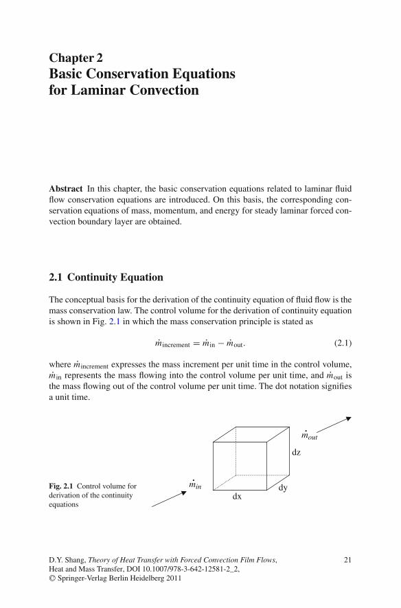
Chapter 2Basic Conservation Equationsfor Laminar Convection
Abstract In this chapter, the basic conservation equations related to laminar fluidflow conservation equations are introduced. On this basis, the corresponding con-servation equations of mass, momentum, and energy for steady laminar forced con-vection boundary layer are obtained.
2.1 Continuity Equation
The conceptual basis for the derivation of the continuity equation of fluid flow is themass conservation law. The control volume for the derivation of continuity equationis shown in Fig. 2.1 in which the mass conservation principle is stated as
mincrement = min − mout. (2.1)
where mincrement expresses the mass increment per unit time in the control volume,min represents the mass flowing into the control volume per unit time, and mout isthe mass flowing out of the control volume per unit time. The dot notation signifiesa unit time.
Fig. 2.1 Control volume forderivation of the continuityequations
dz
dydx
•min
•mout
D.Y. Shang, Theory of Heat Transfer with Forced Convection Film Flows,Heat and Mass Transfer, DOI 10.1007/978-3-642-12581-2_2,C© Springer-Verlag Berlin Heidelberg 2011
21

22 2 Basic Conservation Equations for Laminar Convection
In the control volume, the mass of fluid flow is given by ρ dx dy dz, and the massincrement per unit time in the control volume can be expressed as
mincrement = ∂ρ
∂τdx dy dz. (2.2)
The mass flowing per unit time into the control volume in the x direction is givenby ρwx dy dz. The mass flowing out of the control volume in a unit time in the x
direction is given by
[ρwx + ∂(ρwx )
∂xdx
]dy dz. Thus, the mass increment per unit
time in the x direction in the control volume is given by∂(ρwx )
∂xdx dy dz. Similarly,
the mass increments in the control volume in the y and z directions per unit time are
given by∂(ρwy)
∂ydy dx dz and
∂(ρwz)
∂zdz dx dy, respectively. We thus obtain
mout − min =[∂(ρwx )
∂x+ ∂(ρwy)
∂y+ ∂(ρwz)
∂z
]dx dy dz. (2.3)
With (2.2) and (2.3), (2.1) becomes in Cartesian coordinates:
∂ρ
∂τ+ ∂(ρwx )
∂x+ ∂(ρwy)
∂y+ ∂(ρwz)
∂z= 0, (2.4)
or in the vector notation
∂ρ
∂τ+ ∇ · (ρ →
W ) = 0, (2.5)
where→W = iwx + jwy + kwz is the fluid velocity.
For steady state, the vector and Cartesian forms of the continuity equation aregiven by
∂
∂x(ρwx )+ ∂
∂y(ρwy)+ ∂
∂z(ρwz) = 0, (2.6)
and
∂
∂x(ρwx )+ ∂
∂y(ρwy) = 0, (2.7)
respectively for three- and two- dimensional continuity equations.

2.2 Momentum Equation (Navier–Stokes Equations) 23
2.2 Momentum Equation (Navier–Stokes Equations)
The control volume for derivation of the momentum equation of fluid flow is shownin Fig. 2.2. Take an enclosed surface A that includes the control volume. Meanwhile,
take→F m as mass force per unit mass fluid,
→F m,v as the total mass force in the control
volume,→τ n as surface force per unit mass fluid flow at per area of surface,
→τ n,A as
surface force in the control volume, G increment as momentum increment of the perunit mass fluid flow at unit time, and G increment as momentum increment of the fluidflow per unit time in the volume. According to the momentum law, the momentumincrement of the fluid flow per unit time in the control volume equals the sum oftotal mass force and surface forced in the same volume, as
Gincrement = →F m,v + →
τ n,A. (2.8)
→F m,v,
→τ n,A, and G increment in the control volume are expressed as, respectively,
→F m,v =
∫
Vρ
→Fm dV, (2.9)
→τ n,A =
∫
A
→τ n d A, (2.10)
G increment = D
Dτ
∫
Vρ
→W dV . (2.11)
According to tensor calculation, the right side of (2.10) is expressed as
∫
A
→τ ndA =
∫
V∇ · [τ ]dV , (2.12)
where ∇ · [τ ] is divergence of the shear force tensor.With (2.9), (2.10), (2.11), and (2.12), (2.8) is rewritten as
D
Dτ
∫
Vρ
→W dV =
∫
Vρ
→Fm dV +
∫
V∇ · [τ ]dV , (2.13)
Fig. 2.2 Control volume forderivation of momentumequations
Gx, in•
Gx, out•
dxdy
dzFx

24 2 Basic Conservation Equations for Laminar Convection
i.e.∫
V
⎧⎨⎩
D(ρ→W )
Dτ− ρ
→F −∇ · [τ ]
⎫⎬⎭ dV = 0. (2.14)
Therefore, we have
D(ρ→W )
Dτ= ρ
→F+∇ · [τ ]. (2.15)
This is the Navier–Stokes equations of fluid flow. For Cartesian coordinates, (2.15)can be expressed as
D(ρwx )
Dτ= ∂τxx
∂x+ ∂τyx
∂y+ ∂τzx
∂z+ ρgx , (2.16)
D(ρwy)
Dτ= ∂τxy
∂x+ ∂τyy
∂y+ ∂τzy
∂z+ ρgy, (2.17)
D(ρwz)
Dτ= ∂τxz
∂x+ ∂τyz
∂y+ ∂τzz
∂z+ ρgz, (2.18)
where
τxx = −[
p + 2
3μ
(∂wx
∂x+ ∂wy
∂y+ ∂wz
∂z
)]+ 2μ
∂wx
∂x,
τyy = −[
p + 2
3μ
(∂wx
∂x+ ∂wy
∂y+ ∂wz
∂z
)]+ 2μ
∂wy
∂y,
τzz = −[
p + 2
3μ
(∂wx
∂x+ ∂wy
∂y+ ∂wz
∂z
)]+ 2μ
∂wz
∂z,
τxy = τyx = μ
(∂wy
∂x+ ∂wx
∂y
),
τyz = τzy = μ
(∂wz
∂y+ ∂wy
∂z
),
τzx = τxz = μ
(∂wx
∂z+ ∂wz
∂x
),
gx , gy , and gz are gravity accelerations in x , y, and z directions, respectively.Then, (2.16) to (2.18) become
D(ρwx )
Dτ= − ∂p
∂x+ 2
∂
∂x
(μ∂wx
∂x
)+ ∂
∂y
[μ
(∂wx
∂y+ ∂wy
∂x
)]+ ∂
∂z
[μ
(∂wx
∂ z+ ∂wz
∂x
)]
− ∂
∂x
[2
3μ
((∂wx
∂x+ ∂wy
∂ y+ ∂wz
∂z
)]+ ρgx , (2.19)

2.2 Momentum Equation (Navier–Stokes Equations) 25
D(ρwy)
Dτ= − ∂p
∂y+ ∂
∂x
[μ
(∂wx
∂y+ ∂wy
∂x
)]+ 2
∂
∂y
(μ∂wy
∂y
)+ ∂
∂z
[μ
(∂wy
∂z+ ∂wz
∂y
)]
− ∂
∂y
[2
3μ
(∂wx
∂x+ ∂wy
∂y+ ∂wz
∂z
)]+ ρgy , (2.20)
D(ρwz)
Dτ= − ∂p
∂z+ ∂
∂x
[μ
(∂wx
∂z+ ∂wz
∂x
)]+ ∂
∂y
[μ
(∂wy
∂z+ ∂wz
∂y
)]+ 2
∂
∂z
[μ∂wz
∂z
)
− ∂
∂z
[2
3μ
(∂wx
∂x+ ∂wy
∂y+ ∂wz
∂z
)]+ ρgz (2.21)
For steady state, the momentum equations (2.19) – (2.21) are given as follows,respectively,
ρ
(∂wx
∂xwx + ∂wx
∂ywy + ∂wx
∂zwz
)+ wx
(wx∂ρ
∂x+ wy
∂ρ
∂y+ wz
∂ρ
∂z
)=
− ∂p
∂x+ 2
∂
∂x
(μ∂wx
∂x
)+ ∂
∂y
[μ
(∂wx
∂y+ ∂wy
∂x
)]+ ∂
∂z
[μ
(∂wx
∂z+ ∂wz
∂x
)]
− ∂
∂x
[2
3μ
(∂wx
∂x+ ∂wy
∂y+ ∂wz
∂z
)]+ ρgx , (2.22)
ρ
(∂wy
∂xwx + ∂wy
∂ywy + ∂wy
∂zwz
)+ wy
(wx∂ρ
∂x+ wy
∂ρ
∂y+ wz
∂ρ
∂z
)=
− ∂p
∂y+ ∂
∂x
[μ
(∂wx
∂y+ ∂wy
∂x
)]+ 2
∂
∂y
(μ∂wy
∂y
)+ ∂
∂z
[μ
(∂wy
∂z+ ∂wz
∂y
)]
− ∂
∂y
[2
3μ
(∂wx
∂x+ ∂wy
∂y+ ∂wz
∂z
)]+ ρgy, (2.23)
ρ
(∂wz
∂xwx + ∂wz
∂ywy + ∂wz
∂zwz
)+ wz
(wx∂ρ
∂x+ wy
∂ρ
∂y+ wz
∂ρ
∂z
)=
− ∂p
∂z+ ∂
∂x
[μ
(∂wx
∂z+ ∂wz
∂x
)]+ ∂
∂y
[μ
(∂wy
∂z+ ∂wz
∂y
)]+ 2
∂
∂z
(μ∂wz
∂z
)
− ∂
∂z
[2
3μ
(∂wx
∂x+ ∂wy
∂y+ ∂wz
∂z
)]+ ρgz . (2.24)
Let us compare term ρ(∂wx∂x wx + ∂wx
∂y wy + ∂wx∂z wz
)with term wx
(wx
∂ρ∂x +
wy∂ρ∂y + wz
∂ρ∂z
)in (2.22). In general, derivatives ∂wx
∂x , ∂wx∂y , and ∂wx
∂z are much
larger than the derivatives ∂ρx∂x , ∂ρx
∂y , and ∂ρx∂z , respectively. In this case, the term
wx
(wx
∂ρ∂x + wy
∂ρ∂y + wz
∂ρ∂z
)is omitted, and (2.22) is rewritten as generally

26 2 Basic Conservation Equations for Laminar Convection
ρ
(∂wx
∂xwx + ∂wx
∂ywy + ∂wx
∂zwz
)= −∂p
∂x+ 2
∂
∂x
(μ∂wx
∂x
)
+ ∂
∂y
[μ
(∂wx
∂y+ ∂wy
∂x
)]+ ∂
∂z
[μ
(∂wx
∂z+ ∂wz
∂x
)]
− ∂
∂x
[2
3μ
(∂wx
∂x+ ∂wy
∂y+ ∂wz
∂z
)]+ ρgx . (2.25)
Similarly, in general, (2.23) and (2.24) are rewritten as respectively
ρ
(∂wy
∂xwx + ∂wy
∂ywy + ∂wy
∂zwz
)= −∂p
∂y+ ∂
∂x
[μ
(∂wx
∂y+ ∂wy
∂x
)]
+ 2∂
∂y
(μ∂wy
∂y
)+ ∂
∂z
[μ
(∂wy
∂z+ ∂wz
∂y
)]
− ∂
∂y
[2
3μ
(∂wx
∂x+ ∂wy
∂y+ ∂wz
∂z
)]+ ρgy, (2.26)
ρ
(∂wz
∂xwx + ∂wz
∂ywy + ∂wz
∂zwz
)= −∂p
∂z+ ∂
∂x
[μ
(∂wx
∂z+ ∂wz
∂x
)]
+ ∂
∂y
[μ
(∂wy
∂z+ ∂wz
∂y
)]+ 2
∂
∂z
(μ∂wz
∂z
)
− ∂
∂z
[2
3μ
(∂wx
∂x+ ∂wy
∂y+ ∂wz
∂z
)]+ ρgz (2.27)
2.3 Energy Equation
The control volume for derivation of the energy equation of fluid flow is shown inFig. 2.3. Take an enclosed surface A that includes the control volume. According tothe first law of thermodynamics, we have the following equation:
Fig. 2.3 Control volumefor derivation of the energyequations of fluid flow
Wout
Qin dx
dy
dzΔE
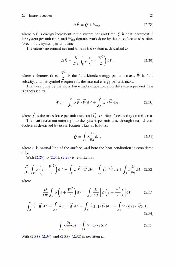
2.3 Energy Equation 27
�E = Q + Wout, (2.28)
where �E is energy increment in the system per unit time, Q is heat increment inthe system per unit time, and Wout denotes work done by the mass force and surfaceforce on the system per unit time.
The energy increment per unit time in the system is described as
�E = D
Dτ
∫
Vρ
(e + W 2
2
)dV , (2.29)
where τ denotes time,W 2
2is the fluid kinetic energy per unit mass, W is fluid
velocity, and the symbol e represents the internal energy per unit mass.The work done by the mass force and surface force on the system per unit time
is expressed as
Wout =∫
Vρ
→F · →
W dV +∫
A
→τn · →
W dA, (2.30)
where→F is the mass force per unit mass and
→τn is surface force acting on unit area.
The heat increment entering into the system per unit time through thermal con-duction is described by using Fourier’s law as follows:
Q =∫
Aλ∂t
∂ndA, (2.31)
where n is normal line of the surface, and here the heat conduction is consideredonly.
With (2.29) to (2.31), (2.28) is rewritten as
D
Dτ
∫
Vρ
(e + W 2
2
)dV =
∫
Vρ
→F · →
W dV +∫
A
→τn · →
W dA +∫
Aλ∂t
∂ndA, (2.32)
where
D
Dτ
∫
Vρ
(e + W 2
2
)dV =
∫
V
D
Dτ
[ρ
(e + W 2
2
)]dV, (2.33)
∫
A
→τn · →
W dA =∫
A
→n [τ ] · →
W dA =∫
A
→n ([τ ] · →
W )dA =∫
v
∇ · ([τ ] · →W )dV,
(2.34)
∫
Aλ∂t
∂ndA =
∫
V∇ · (λ∇t)dV . (2.35)
With (2.33), (2.34), and (2.35), (2.32) is rewritten as
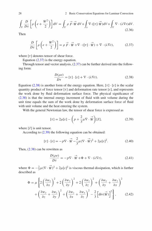
28 2 Basic Conservation Equations for Laminar Convection
∫
V
D
Dτ
[ρ
(e + W 2
2
)]dV =
∫
Vρ
→F ·→
W dV +∫
v
∇·([τ ]·→W )dV +
∫
V∇ · (λ∇t)dV .
(2.36)Then
D
Dτ
[ρ
(e + W 2
2
)]= ρ
→F · →
W +∇ · ([τ ] · →W )+ ∇ · (λ∇t), (2.37)
where [τ ] denotes tensor of shear force.Equation (2.37) is the energy equation.Through tensor and vector analysis, (2.37) can be further derived into the follow-
ing form:
D(ρe)
Dτ= [τ ] · [ε] + ∇ · (λ∇t). (2.38)
Equation (2.38) is another form of the energy equation. Here, [τ ] · [ε] is the scalarquantity product of force tensor [τ ] and deformation rate tensor [ε], and representsthe work done by fluid deformation surface force. The physical significance of(2.38) is that the internal energy increment of fluid with unit volume during theunit time equals the sum of the work done by deformation surface force of fluidwith unit volume and the heat entering the system.
With the general Newtonian law, the tensor of shear force is expressed as
[τ ] = 2μ[ε] −(
p + 2
3μ∇ · →
W
)[I ], (2.39)
where [I ] is unit tensor.According to (2.39) the following equation can be obtained:
[τ ] · [ε] = −p∇ · →W −2
3μ(∇ · →
W )2 + 2μ[ε]2. (2.40)
Then, (2.38) can be rewritten as
D(ρe)
Dτ= −p∇ · →
W +�+ ∇ · (λ∇t), (2.41)
where � = − 23μ(∇ · →
W )2 + 2μ[ε]2 is viscous thermal dissipation, which is furtherdescribed as
� = μ
{2
(∂wx
∂x
)2
+ 2
(∂wy
∂y
)2
+ 2
(∂wz
∂z
)2
+(∂wx
∂y+ ∂wy
∂x
)2
+(∂wy
∂z+ ∂wz
∂y
)2
+(∂wz
∂x+ ∂wx
∂z
)2
− 2
3
[div(
→W )]2}
, (2.42)

2.3 Energy Equation 29
where
div(→W ) = ∂wx
∂x+ ∂wy
∂y+ ∂wz
∂z.
According to continuity equation (2.5), we have
∇ · →W = − 1
ρ
Dρ
Dτ= ρ
D
Dτ
(1
ρ
).
With the above equation, (2.41) is changed into the following form:
[D(ρe)
Dτ+ pρ
D
Dτ
(1
ρ
)]= �+ ∇ · (λ∇t). (2.43)
According to thermodynamics equation of fluid, we have
D(ρh)
Dτ= D(ρe)
Dτ+ pρ
D
Dτ
(1
ρ
)+ Dp
Dτ. (2.44)
Then, Equation (2.43) can be expressed as the following enthalpy form:
D(ρh)
Dτ= Dp
Dτ+�+ ∇ · (λ∇t), (2.45)
or
D(ρcp · t)
Dτ= Dp
Dτ+�+ ∇ · (λ∇t), (2.46)
where h = cp · t , while cp is specific heat.In Cartesian form, the energy (2.46) can be rewritten as
∂(ρcp · t)
∂τ+ wx
∂(ρcp · t)
∂x+ wy
∂(ρcp · t)
∂y+ wz
∂(ρcp · t)
∂z
= D P
Dτ+ ∂
∂x
(λ∂t
∂x
)+ ∂
∂y
(λ∂t
∂y
)+ ∂
∂z
(λ∂t
∂z
)+�.
(2.47)
For steady state, the three-dimensional Cartesian form of the energy equa-tion (2.47) is changed into
wx∂(ρcpt)
∂x+ wy
∂(ρcpt)
∂y+ wz
∂(ρcpt)
∂z= ∂
∂x
(λ∂t
∂x
)+ ∂
∂y
(λ∂t
∂y
)
+ ∂
∂z
(λ∂t
∂z
)+�. (2.48)

30 2 Basic Conservation Equations for Laminar Convection
Above equation is usually approximately rewritten as
ρ
[wx∂(cp · t)
∂x+ wy
∂(cp · t)
∂y+ wz
∂(cp · t)
∂z
]= ∂
∂x
(λ∂t
∂x
)+ ∂
∂y
(λ∂t
∂y
)
+ ∂
∂z
(λ∂t
∂z
)+�, (2.49)
where the temperature-dependence of density is ignored.For steady state, the two-dimensional Cartesian form of the energy equa-
tion (2.48) is changed into
wx∂(ρcpt)
∂x+ wy
∂(ρcpt)
∂y= ∂
∂x
(λ∂t
∂x
)+ ∂
∂y
(λ∂t
∂y
)+�. (2.50)
Above equation is usually approximately rewritten as
ρ
[wx∂(cpt)
∂x+ wy
∂(cpt)
∂y
]= ∂
∂x
(λ∂t
∂xt
)+ ∂
∂y
(λ∂t
∂y
)+�. (2.51)
With the two-dimensional form, the viscous thermal dissipation is
� = μ
{2
(∂wx
∂x
)2
+ 2
(∂wy
∂y
)2
+(∂wx
∂y+ ∂wy
∂x
)2
− 2
3
[div(
→W )]2}
, (2.52)
where
div(→W ) = ∂wx
∂x+ ∂wy
∂y.
2.4 Governing Partial Differential Equations of Laminar ForcedConvection Boundary Layers with Consideration of VariablePhysical Properties
2.4.1 Principle of the Quantitative Grade Analysis
The general governing partial differential equations can be transformed to therelated boundary layer equations. In fact, the only difference between the gov-erning equations of free and forced convection is that buoyant force is onlyconsidered in the related momentum equation of free convection. Before thequantitative grade analysis, it is necessary to define its analytical standard. Anormal quantitative grade is regarded as {1}, i.e. unit quantity grade, a verysmall quantitative grade is regarded as {δ}, even very small quantitative grade
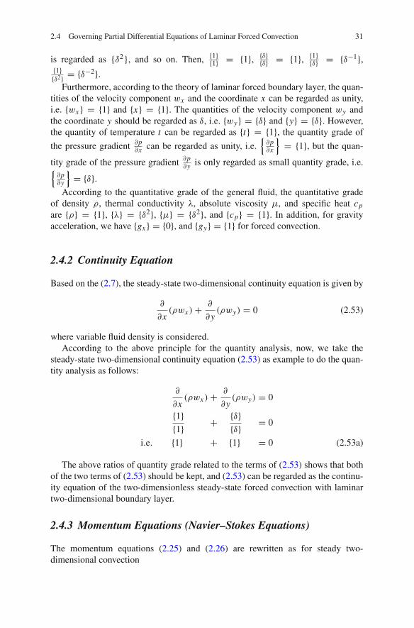
2.4 Governing Partial Differential Equations of Laminar Forced Convection 31
is regarded as {δ2}, and so on. Then, {1}{1} = {1}, {δ}
{δ} = {1}, {1}{δ} = {δ−1},
{1}{δ2} = {δ−2}.
Furthermore, according to the theory of laminar forced boundary layer, the quan-tities of the velocity component wx and the coordinate x can be regarded as unity,i.e. {wx } = {1} and {x} = {1}. The quantities of the velocity component wy andthe coordinate y should be regarded as δ, i.e. {wy} = {δ} and {y} = {δ}. However,the quantity of temperature t can be regarded as {t} = {1}, the quantity grade of
the pressure gradient ∂p∂x can be regarded as unity, i.e.
{∂p∂x
}= {1}, but the quan-
tity grade of the pressure gradient ∂p∂y is only regarded as small quantity grade, i.e.{
∂p∂y
}= {δ}.
According to the quantitative grade of the general fluid, the quantitative gradeof density ρ, thermal conductivity λ, absolute viscosity μ, and specific heat cp
are {ρ} = {1}, {λ} = {δ2}, {μ} = {δ2}, and {cp} = {1}. In addition, for gravityacceleration, we have {gx } = {0}, and {gy} = {1} for forced convection.
2.4.2 Continuity Equation
Based on the (2.7), the steady-state two-dimensional continuity equation is given by
∂
∂x(ρwx )+ ∂
∂y(ρwy) = 0 (2.53)
where variable fluid density is considered.According to the above principle for the quantity analysis, now, we take the
steady-state two-dimensional continuity equation (2.53) as example to do the quan-tity analysis as follows:
∂
∂x(ρwx )+ ∂
∂y(ρwy) = 0
{1}{1} + {δ}
{δ} = 0
i.e. {1} + {1} = 0 (2.53a)
The above ratios of quantity grade related to the terms of (2.53) shows that bothof the two terms of (2.53) should be kept, and (2.53) can be regarded as the continu-ity equation of the two-dimensionless steady-state forced convection with laminartwo-dimensional boundary layer.
2.4.3 Momentum Equations (Navier–Stokes Equations)
The momentum equations (2.25) and (2.26) are rewritten as for steady two-dimensional convection
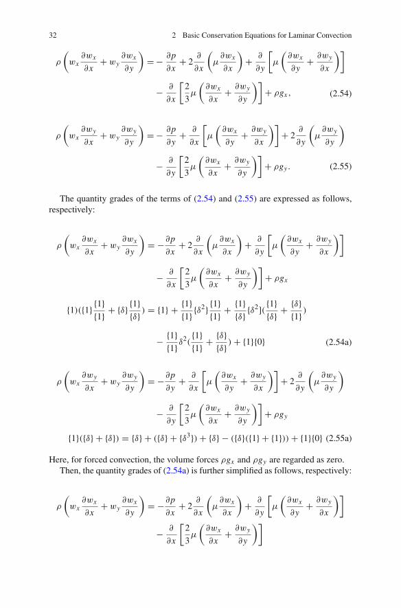
32 2 Basic Conservation Equations for Laminar Convection
ρ
(wx∂wx
∂x+ wy
∂wx
∂y
)= − ∂p
∂x+ 2
∂
∂x
(μ∂wx
∂x
)+ ∂
∂y
[μ
(∂wx
∂y+ ∂wy
∂x
)]
− ∂
∂x
[2
3μ
(∂wx
∂x+ ∂wy
∂y
)]+ ρgx , (2.54)
ρ
(wx∂wy
∂x+ wy
∂wy
∂y
)= − ∂p
∂y+ ∂
∂x
[μ
(∂wx
∂y+ ∂wy
∂x
)]+ 2
∂
∂y
(μ∂wy
∂y
)
− ∂
∂y
[2
3μ
(∂wx
∂x+ ∂wy
∂y
)]+ ρgy . (2.55)
The quantity grades of the terms of (2.54) and (2.55) are expressed as follows,respectively:
ρ
(wx∂wx
∂x+ wy
∂wx
∂y
)= −∂p
∂x+ 2
∂
∂x
(μ∂wx
∂x
)+ ∂
∂y
[μ
(∂wx
∂y+ ∂wy
∂x
)]
− ∂
∂x
[2
3μ
(∂wx
∂x+ ∂wy
∂y
)]+ ρgx
{1)({1} {1}{1} + {δ} {1}
{δ} ) = {1} + {1}{1} {δ
2} {1}{1} + {1}
{δ} {δ2]( {1}{δ} + {δ}
{1} )
− {1}{1}δ
2({1}{1} + {δ}
{δ} )+ {1}{0} (2.54a)
ρ
(wx∂wy
∂x+ wy
∂wy
∂y
)= −∂p
∂y+ ∂
∂x
[μ
(∂wx
∂y+ ∂wy
∂x
)]+ 2
∂
∂y
(μ∂wy
∂y
)
− ∂
∂y
[2
3μ
(∂wx
∂x+ ∂wy
∂y
)]+ ρgy
{1}({δ} + {δ}) = {δ} + ({δ} + {δ3})+ {δ} − ({δ}({1} + {1}))+ {1}{0} (2.55a)
Here, for forced convection, the volume forces ρgx and ρgy are regarded as zero.Then, the quantity grades of (2.54a) is further simplified as follows, respectively:
ρ
(wx∂wx
∂x+ wy
∂wx
∂y
)= −∂p
∂x+ 2
∂
∂x
(μ∂wx
∂x
)+ ∂
∂y
[μ
(∂wx
∂y+ ∂wy
∂x
)]
− ∂
∂x
[2
3μ
(∂wx
∂x+ ∂wy
∂y
)]

2.4 Governing Partial Differential Equations of Laminar Forced Convection 33
{1)({1} + {1}) = {1} + {δ2} + {1} + {δ2} − ({δ2} + {δ2}) (2.54b)
Observing the quantity grades in (2.54a) it is found that the terms 2 ∂∂x
(μ∂wx∂x
),
∂wy∂x in term ∂
∂y
[μ(∂wx∂y + ∂wy
∂x
)], ∂∂x
[23μ(∂wx∂x + ∂wy
∂y
)]are very small and can be
ignored. Then, (2.54a) is simplified as follows:
ρ
(wx∂wx
∂x+ wy
∂wx
∂y
)= −∂p
∂x+ ∂
∂y
[μ
(∂wx
∂y
)]. (2.56)
Comparing the quantity grades of (2.55a) with those of (2.54b), it is found that thequantity grades of (2.55a) are very small. Then, (2.55) can be ignored, and only(2.56) is taken as the momentum equation of steady-state forced convection withtwo-dimensional boundary layer.
2.4.4 Energy Equations
The quantity grades of the terms of (2.51) for laminar two-dimensional energy equa-tion is expressed as
ρ
[wx∂(cpt)
∂x+ wy
∂(cpt)
∂y
]= ∂
∂x
(λ∂t
∂x
)+ ∂
∂y
(λ∂t
∂y
)+�
{1}[{1} · {1}
{1} + {δ} · {1}{δ}]
= {1}{1}(δ2 {1}
{1})
+ {1}{δ} δ
2 {1}{δ}
(2.51a)
The quantity grade of (2.51a) is simplified to
ρ
[wx∂(cpt)
∂x+ wy
∂(cpt)
∂y
]= ∂
∂x
(λ∂t
∂x
)+ ∂
∂y
(λ∂t
∂y
)+�
{1}[{1} + {1}·] = {1}(δ2} + {1})(2.51b)
With the quantity grade analysis from (2.51b), it is seen that the term ∂∂x
(λ ∂t∂x
)is
very small compared with other terms, and then can be omitted from the equation.Then, the energy equation for steady-state forced convection with two-dimensionallaminar boundary layer is simplified to
ρ
[wx∂(cpt)
∂x+ wy
∂(cpt)
∂y
]= ∂
∂y
(λ∂t
∂y
)+�. (2.57)
Now, we analyze the viscous thermal dissipation �. According to (2.52), � isthe following equation for the laminar stead state convection:

34 2 Basic Conservation Equations for Laminar Convection
� = μ
{2
(∂wx
∂x
)2
+ 2
(∂wy
∂y
)2
+(∂wx
∂y+ ∂wy
∂x
)2
− 2
3
(∂wx
∂x+ ∂wy
∂y
)2}.
(2.52a)
With quantity grade analysis, the right side of (2.52a) is expressed as
� = μ
{2
(∂wx
∂x
)2
+ 2
(∂wy
∂y
)2
+(∂wx
∂y+ ∂wy
∂x
)2
− 2
3
(∂wx
∂x+ ∂wy
∂y
)2}
{δ2}(( {1}
{1})2
+( {δ}
{δ})2
+( {1}
{δ} + {δ}{1})2
−( {1}
{1} + {δ}{δ})2)
The quantity grade of the above equation is equivalent to
{δ2}(
{1} + {1} +( {1}
{δ2} + {δ2})
− ({1} + {1})2)
(2.52b)
With the quantity grade comparison, it is found that only the term μ(∂wx∂y
)2may
be kept. Then, for the stead state forced convection with two-dimensional boundarylayer, the viscous thermal dissipation is simplified to
� = μ
(∂wx
∂y
)2
. (2.52c)
With (2.52c), (2.57) is changed to the following equation
ρ
[wx∂(cpt)
∂x+ wy
∂(cpt)
∂y
]= ∂
∂y
(λ∂t
∂y
)+ μ
(∂wx
∂y
)2
(2.58)
as the steady-state energy equation with laminar forced convection for two-dimensional boundary layer.
In a later chapter, I will investigate the effect of the viscous thermal dissipationon heat transfer of laminar forced convection.
Now the basic governing partial differential equations for description of mass,momentum, and energy conservation of two-dimensional laminar steady-stateforced convection boundary layers are shown as follows with consideration viscousthermal dissipation and variable physical properties:
∂
∂x(ρwx )+ ∂
∂y(ρwy) = 0, (2.53)
ρ
(wx∂wx
∂x+ wy
∂wx
∂y
)= −∂p
∂x+ ∂
∂y
[μ
(∂wx
∂y
)], (2.56)
ρ
[wx∂(cpt)
∂x+ wy
∂(cpt)
∂y
]= ∂
∂y
(λ∂t
∂y
)+ μ
(∂wx
∂y
)2
. (2.58)

2.4 Governing Partial Differential Equations of Laminar Forced Convection 35
Suppose a bulk flow with the velocity wx,∞ beyond the boundary layer, (2.56) issimplified to the following form:
wx,∞∂wx,∞∂x
= − 1
ρ
dp
dx,
i.e.
dp
dx= −ρwx,∞
∂wx,∞∂x
.
Then (2.56) is changed to
ρ
(wx∂wx
∂x+ wy
∂wx
∂y
)= ρwx,∞
∂wx,∞∂x
+ ∂
∂y
(μ
(∂wx
∂y
))(2.56a)
Obviously, if the main stream velocity wx,∞ is constant, i.e. ∂wx,∞∂x = 0, (2.56a) is
identical to the following equations:
ρ
(wx∂wx
∂x+ wy
∂wx
∂y
)= ∂
∂y
[μ
(∂wx
∂y
)]. (2.56b)
For rigorous solutions of the governing equations, the fluid temperature-dependent properties, such as density ρ, absolute viscosity μ, specific heat cp,and thermal conductivity λ will be considered in the successive chapters of thisbook.
The laminar forced convection with two-dimensional boundary layer belongs totwo-point boundary value problem, which is the basis of three-point boundary valueproblem for film condensation.
Obviously, the basic governing partial differential equations for mass, momen-tum, and energy conservation of two-dimensional laminar steady-state forced con-vection boundary layers with considering viscous thermal dissipation but ignoringthe variable physical properties are obtained as based on (2.53), (2.56), and (2.58):
∂wx
∂x+ ∂wy
∂y= 0 (2.59)
wx∂wx
∂x+ wy
∂wx
∂y= − 1
ρ
∂p
∂x+ ν
∂2wx
∂y2(2.60)
with − 1
ρ
dp
dx= wx,∞
∂wx,∞∂x
[wx
∂t
∂x+ wy
∂t
∂y
]= ν
Pr
∂2t
∂2+ (ν/cp
) (∂wx
∂y
)2
. (2.61)
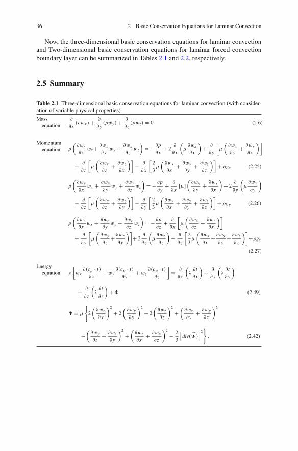
36 2 Basic Conservation Equations for Laminar Convection
Now, the three-dimensional basic conservation equations for laminar convectionand Two-dimensional basic conservation equations for laminar forced convectionboundary layer can be summarized in Tables 2.1 and 2.2, respectively.
2.5 Summary
Table 2.1 Three-dimensional basic conservation equations for laminar convection (with consider-ation of variable physical properties)
Massequation
∂
∂x(ρwx )+ ∂
∂y(ρwy)+ ∂
∂z(ρwz) = 0 (2.6)
Momentumequation ρ
(∂wx
∂xwx + ∂wx
∂ywy + ∂wx
∂zwz
)= − ∂p
∂x+ 2
∂
∂x
(μ∂wx
∂x
)+ ∂
∂y
[μ
(∂wx
∂y+ ∂wy
∂x
)]
+ ∂
∂z
[μ
(∂wx
∂z+ ∂wz
∂x
)]− ∂
∂x
[2
3μ
(∂wx
∂x+ ∂wy
∂y+ ∂wz
∂z
)]+ ρgx (2.25)
ρ
(∂wy
∂xwx + ∂wy
∂ywy + ∂wy
∂zwz
)= − ∂p
∂y+ ∂
∂x[μ]
(∂wx
∂y+ ∂wy
∂x
)+ 2
∂
∂y
(μ∂wy
∂y
)
+ ∂
∂z
[μ
(∂wy
∂z+ ∂wz
∂y
)]− ∂
∂y
[2
3μ
(∂wx
∂x+ ∂wy
∂y+ ∂wz
∂z
)]+ ρgy (2.26)
ρ
(∂wz
∂xwx + ∂wz
∂ywy + ∂wz
∂zwz
)= − ∂p
∂z+ ∂
∂x
[μ
(∂wx
∂z+ ∂wz
∂x
)]
+ ∂
∂y
[μ
(∂wy
∂z+ ∂wz
∂y
)]+ 2
∂
∂z
(μ∂wz
∂z
)− ∂
∂z
[2
3μ
(∂wx
∂x+ ∂wy
∂y+ ∂wz
∂z
)]+ρgz
(2.27)
Energyequation ρ
[wx∂(cp · t)
∂x+ wy
∂(cp · t)
∂y+ wz
∂(cp · t)
∂z
]= ∂
∂x
(λ∂t
∂x
)+ ∂
∂y
(λ∂t
∂y
)
+ ∂
∂z
(λ∂t
∂z
)+� (2.49)
� = μ
{2
(∂wx
∂x
)2
+ 2
(∂wy
∂y
)2
+ 2
(∂wz
∂z
)2
+(∂wx
∂y+ ∂wy
∂x
)2
+(∂wy
∂z+ ∂wz
∂y
)2
+(∂wz
∂x+ ∂wx
∂z
)2
− 2
3
[div(
→W )]2}
, (2.42)
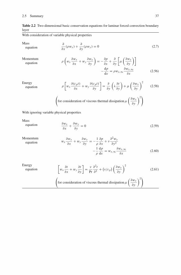
2.5 Summary 37
Table 2.2 Two-dimensional basic conservation equations for laminar forced convection boundarylayer
With consideration of variable physical properties
Massequation
∂
∂x(ρwx )+ ∂
∂y(ρwy) = 0 (2.7)
Momentumequation ρ
(wx∂wx
∂x+ wy
∂wx
∂y
)= − ∂p
∂x+ ∂
∂y
[μ
(∂wx
∂y
)]
−dp
dx= ρwx,∞
∂wx,∞∂x
(2.56)
Energyequation ρ
[wx∂(cpt)
∂x+ wy
∂(cpt)
∂y
]= ∂
∂y
(λ∂t
∂y
)+ μ
(∂wx
∂y
)2
(2.58)
(for consideration of viscous thermal dissipationμ
(∂wx
∂y
)2)
With ignoring variable physical properties
Massequation ∂wx
∂x+ ∂wy
∂y= 0 (2.59)
Momentumequation wx
∂wx
∂x+ wy
∂wx
∂y= − 1
ρ
∂p
∂x+ ν
∂2wx
∂y2
− 1
ρ
dp
dx= wx,∞
∂wx,∞∂x
(2.60)
Energyequation
[wx
∂t
∂x+ wy
∂t
∂y
]= ν
Pr
∂2t
∂2+ (ν/cp
) ( ∂wx
∂y
)2
(2.61)
(for consideration of viscous thermal dissipationμ
(∂wx
∂y
)2)


Chapter 3Review of Falkner-Skan Type Transformationfor Laminar Forced Convection Boundary Layer
Abstract In this chapter, the traditional Falkner–Skan-type transformation forlaminar forced convection boundary layer is reviewed. The typical two-dimensionalbasic conservation equations for laminar forced convection boundary layer are takenas example for derivation of the related similarity variables for Falkner–Skan-typetransformation. By means of the stream function and the procedure with the methodfor group theory, the similarity intermediate function variable f(η) is induced. Then,the velocity components are transformed to the related functions with the similarityintermediate function variable f(η). On this basis, partial differential momentumequation of the forced convection boundary layer is transformed to related ordinaryequation. At last, the limitations of the Falkner–Skan-type transformation are ana-lyzed in detail.
3.1 Introduction
For solution of the laminar boundary layer problem, Falkner and Skan [1] proposedtheir similarity method in 1931, Now, the widely applied similarity analysis andtransformation for the laminar convection and film flows is based on the Falkner-Skan type transformation. So far, the Falkner-Skan type transformation has beencollected in numerous publications, but only some of them such as [2–14] are listedhere for saving space. So, before the presentation of my related new similarity anal-ysis method in this book for laminar forced convection and film flows, it is necessaryhere to review briefly the Falkner-Skan type similarity method.
3.2 Basic Conservation Equations
Based on (2.59) to (2.61), the typical two-dimensional basic conservation equationsfor laminar forced convection boundary layer are shown below with ignoring vari-able physical properties and viscous thermal dissipation:
∂
∂x(wx )+ ∂
∂y(wy) = 0, (3.1)
D.Y. Shang, Theory of Heat Transfer with Forced Convection Film Flows,Heat and Mass Transfer, DOI 10.1007/978-3-642-12581-2_3,C© Springer-Verlag Berlin Heidelberg 2011
39

40 3 Review of Falkner-Skan Type Transformation
wx∂wx
∂x+ wy
∂wx
∂y= − 1
ρ f
∂p
∂x+ ν f
∂2wx
∂y2 , (3.2)
− 1
ρ f
dp
dx= wx,∞
∂wx,∞∂x
,
wx∂t
∂x+ wy
∂t
∂y= ν f
Pr f
∂2t
∂y2, (3.3)
with the boundary condition equations
y = 0: wx = 0, wy = 0, t = tw, (3.4)
y → ∞ : wx = wx,∞, t = t∞. (3.5)
Here,wx andwy are velocity components of the fluids in x and y directions, respec-tively, wx,∞ is the constant mainstream velocity, t is temperature. While the sub-script “ f ” is induced in the equations for inferring in particular to the constant phys-
ical properties with the average temperature of boundary layer, i.e. t f = tw + t∞2
(the same below). Here, (3.1), (3.2), and (3.3) will be taken as a basis for introduc-tion of the Falkner-Skan type transformation method.
3.3 Derivation Review of Similarity Variables of Falkner-SkanTransformation on Laminar Forced Convection
For introducing the Falkner-Skan type transformation, first the solution of the aboveequations is expressed as the following form:
wx
wx,∞= φ1(x, y), (3.6)
t − t∞tw − t∞
= φ2(x, y). (3.7)
In some special cases, (3.6) and (3.7) can be rewritten as
wx
wx,∞= φ1(η), (3.8)
t − t∞tw − t∞
= φ2(η), (3.9)
where η is dimensionless similarity variable, a function of x and y. Later, it will be
shown that η is proportional toy
δ(x)where δ(x) is some function of x . Then, the
number of independent coordinate variables can be reduced from two to one.

3.3 Derivation Review of Similarity Variables of Falkner-Skan Transformation 41
A prerequisite of the Falkner-Skan transformation is the derivation of the simi-larity variables. The typical method for this procedure is group theory, which wasdiscussed at length by Hansen [15] and Na [16]. For application of this method, astream function ψ(x, y) is assumed to satisfy the equation (3.1), i..e
wx = ∂ψ
∂y, wy = −∂ψ
∂x(3.10)
Using (3.10), (3.2) is transformed into
∂ψ
∂y
∂2ψ
∂x∂y− ∂ψ
∂x
∂2ψ
∂y2= wx,∞
dwx,∞dx
+ ν∂3ψ
∂y3(3.11)
Subsequently, (3.11) is solved by using the group theory. For this purpose, it isimportant to introduce the following linear transformation:
x = Aa1 x, y = Aa2 y, ψ = Aa3ψ, wx,∞ = Aa4wx,∞, (3.12)
where a1, a2, a3 and a4 are constant, and A is the transformation parameter.With (3.12), (3.11) can be rewritten as
A2a3−a1−2a2
(∂ψ
∂ y
∂2ψ
∂x∂ y− ∂ψ
∂x
∂2ψ
∂x2
)= A2a4−a1wx,∞
dwx,∞dx
+ νAa3−3a2∂3ψ
∂ y3 .
(3.13)
From (3.13), due to the constancy of the variables, we compare the exponents of Ain each of the terms and obtain
2a3 − a1 − 2a2 = 2a4 − a1 = a3 − 3a2. (3.14)
The incomplete solution of (3.14) is
a3 = a1 − a2, a4 = a3 − a2. (3.15)
Defining a new variable a = a2
a1, (3.15) can be rewritten as
a3
a1= 1 − a,
a4
a1= 2
a3
a1− 1 = 1 − 2a. (3.16)
From (3.12) we get
A =( x
x
) 1a1 =(
y
y
) 1a2 =(ψ
ψ
) 1a3 =(wx,∞wx,∞
) 1a4. (3.17)

42 3 Review of Falkner-Skan Type Transformation
Using (3.16), (3.17) can be transformed as
y
xa= y
xa ,ψ
x1−a= ψ
(x)1−a,
wx,∞x1−2a
= wx,∞(x)1−2a
. (3.18)
These combined variables in (3.18) are called absolute variables in the linear trans-formation of (3.12). According to Morgan theorem [15], if the boundary conditionsof the velocity field of (3.4) and (3.5) can also be transformed, these absolute vari-ables are similarity variables. We set now
η = y
xa , f (η) = ψ
x1−a, (3.19)
h(η) = wx,∞x1−2a
= constant = C. (3.20)
Suppose the main stream velocity wx,∞ is only function of x , then it is never incon-stant function of η. Because variable y is induced in η, h(η) must be constant.
The second part of (3.19) can be rewritten as
ψ = x1−a f (η)xa
xa= x1−2a xa f (η).
With (3.20) this equation can be transformed into
ψ = wx,∞C
xa f (η). (3.21)
By using the first equation of (3.10), the first equation of (3.19), and (3.21), wx isrewritten as
wx = ∂ψ
∂y= ∂ψ
∂η
∂η
∂y= wx,∞
C
∂ f (η)
∂η,
or
wx
wx,∞= f ′(η)
C. (3.22)
Now, we set m = 1 − 2a. From (3.20) we obtain
wx,∞ = Cxm . (3.23)
Using (3.23) the first equation of (3.19) will be transformed to
η = y
x (1−m)/2=(wx,∞
Cx
)1/2y =(wx,∞x
C
)1/2 y
x.
Replace C with 2ν f , the above equation is
η = y
x
(wx,∞x
2ν f
)1/2
= y
x
(1
2Rex, f
)1/2
(3.24)
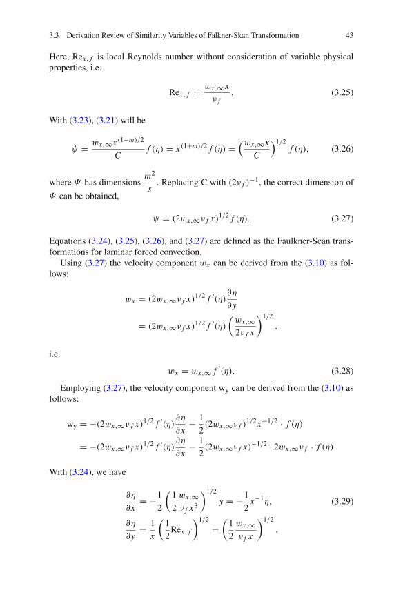
3.3 Derivation Review of Similarity Variables of Falkner-Skan Transformation 43
Here, Rex, f is local Reynolds number without consideration of variable physicalproperties, i.e.
Rex, f = wx,∞x
ν f. (3.25)
With (3.23), (3.21) will be
ψ = wx,∞x (1−m)/2
Cf (η) = x (1+m)/2 f (η) =
(wx,∞x
C
)1/2f (η), (3.26)
where Ψ has dimensionsm2
s. Replacing C with (2ν f )
−1, the correct dimension of
Ψ can be obtained,
ψ = (2wx,∞ν f x)1/2 f (η). (3.27)
Equations (3.24), (3.25), (3.26), and (3.27) are defined as the Faulkner-Scan trans-formations for laminar forced convection.
Using (3.27) the velocity component wx can be derived from the (3.10) as fol-lows:
wx = (2wx,∞ν f x)1/2 f ′(η)∂η∂y
= (2wx,∞ν f x)1/2 f ′(η)(wx,∞2ν f x
)1/2
,
i.e.
wx = wx,∞ f ′(η). (3.28)
Employing (3.27), the velocity component wy can be derived from the (3.10) asfollows:
wy = −(2wx,∞ν f x)1/2 f ′(η) ∂η∂x
− 1
2(2wx,∞ν f )
1/2x−1/2 · f (η)
= −(2wx,∞ν f x)1/2 f ′(η) ∂η∂x
− 1
2(2wx,∞ν f x)−1/2 · 2wx,∞ν f · f (η).
With (3.24), we have
∂η
∂x= −1
2
(1
2
wx,∞ν f x3
)1/2
y = −1
2x−1η, (3.29)
∂η
∂y= 1
x
(1
2Rex, f
)1/2
=(
1
2
wx,∞ν f x
)1/2
.
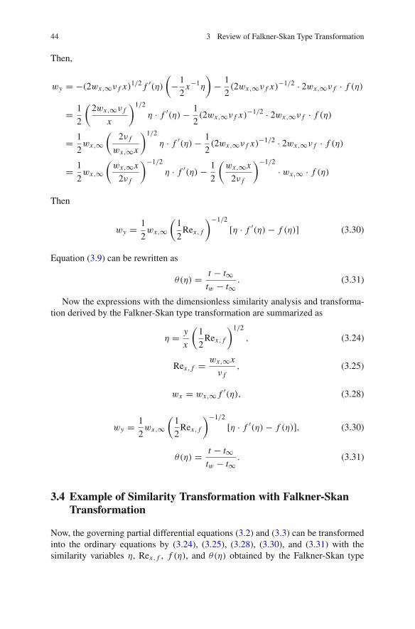
44 3 Review of Falkner-Skan Type Transformation
Then,
wy = −(2wx,∞ν f x)1/2 f ′(η)(
−1
2x−1η
)− 1
2(2wx,∞ν f x)−1/2 · 2wx,∞ν f · f (η)
= 1
2
(2wx,∞ν f
x
)1/2
η · f ′(η)− 1
2(2wx,∞ν f x)−1/2 · 2wx,∞ν f · f (η)
= 1
2wx,∞
(2ν f
wx,∞x
)1/2
η · f ′(η)− 1
2(2wx,∞ν f x)−1/2 · 2wx,∞ν f · f (η)
= 1
2wx,∞
(wx,∞x
2ν f
)−1/2
η · f ′(η)− 1
2
(wx,∞x
2ν f
)−1/2
· wx,∞ · f (η)
Then
wy = 1
2wx,∞
(1
2Rex, f
)−1/2
[η · f ′(η)− f (η)] (3.30)
Equation (3.9) can be rewritten as
θ(η) = t − t∞tw − t∞
. (3.31)
Now the expressions with the dimensionless similarity analysis and transforma-tion derived by the Falkner-Skan type transformation are summarized as
η = y
x
(1
2Rex, f
)1/2
, (3.24)
Rex, f = wx,∞x
ν f, (3.25)
wx = wx,∞ f ′(η), (3.28)
wy = 1
2wx,∞
(1
2Rex, f
)−1/2
[η · f ′(η)− f (η)], (3.30)
θ(η) = t − t∞tw − t∞
. (3.31)
3.4 Example of Similarity Transformation with Falkner-SkanTransformation
Now, the governing partial differential equations (3.2) and (3.3) can be transformedinto the ordinary equations by (3.24), (3.25), (3.28), (3.30), and (3.31) with thesimilarity variables η, Rex, f , f (η), and θ(η) obtained by the Falkner-Skan type
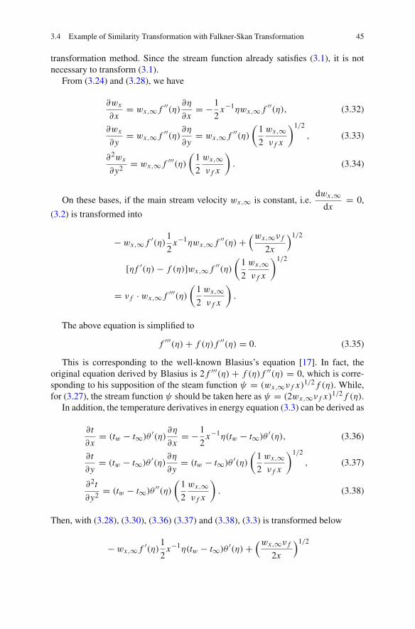
3.4 Example of Similarity Transformation with Falkner-Skan Transformation 45
transformation method. Since the stream function already satisfies (3.1), it is notnecessary to transform (3.1).
From (3.24) and (3.28), we have
∂wx
∂x= wx,∞ f ′′(η) ∂η
∂x= −1
2x−1ηwx,∞ f ′′(η), (3.32)
∂wx
∂y= wx,∞ f ′′(η)∂η
∂y= wx,∞ f ′′(η)
(1
2
wx,∞ν f x
)1/2
, (3.33)
∂2wx
∂y2= wx,∞ f ′′′(η)
(1
2
wx,∞ν f x
). (3.34)
On these bases, if the main stream velocity wx,∞ is constant, i.e.dwx,∞
dx= 0,
(3.2) is transformed into
− wx,∞ f ′(η)1
2x−1ηwx,∞ f ′′(η)+
(wx,∞ν f
2x
)1/2
[η f ′(η)− f (η)]wx,∞ f ′′(η)(
1
2
wx,∞ν f x
)1/2
= ν f · wx,∞ f ′′′(η)(
1
2
wx,∞ν f x
).
The above equation is simplified to
f ′′′(η)+ f (η) f ′′(η) = 0. (3.35)
This is corresponding to the well-known Blasius’s equation [17]. In fact, theoriginal equation derived by Blasius is 2 f ′′′(η) + f (η) f ′′(η) = 0, which is corre-sponding to his supposition of the steam function ψ = (wx,∞ν f x)1/2 f (η). While,for (3.27), the stream function ψ should be taken here as ψ = (2wx,∞ν f x)1/2 f (η).
In addition, the temperature derivatives in energy equation (3.3) can be derived as
∂t
∂x= (tw − t∞)θ ′(η) ∂η
∂x= −1
2x−1η(tw − t∞)θ ′(η), (3.36)
∂t
∂y= (tw − t∞)θ ′(η)∂η
∂y= (tw − t∞)θ ′(η)
(1
2
wx,∞ν f x
)1/2
, (3.37)
∂2t
∂y2= (tw − t∞)θ ′′(η)
(1
2
wx,∞ν f x
). (3.38)
Then, with (3.28), (3.30), (3.36) (3.37) and (3.38), (3.3) is transformed below
− wx,∞ f ′(η)1
2x−1η(tw − t∞)θ ′(η)+
(wx,∞ν f
2x
)1/2

46 3 Review of Falkner-Skan Type Transformation
[η · f ′(η)− f (η)](tw − t∞)θ ′(η)(
1
2
wx,∞ν f x
)1/2
= ν f
Pr f(tw − t∞)θ ′′(η)
(1
2
wx,∞ν f x
)
Simplifying this equation, we obtain
− f ′(η)θ ′(η)η + [η · f ′(η)− f (η)]θ ′(η) = 1
Pr fθ ′′(η),
i.e.
θ ′′(η)+ Pr f f (η)θ ′(η) = 0. (3.39)
Now, the similarity governing ordinary equations for laminar forced convectiontransformed by Falkner-Skan transformation are collected below:
f ′′′(η)+ f (η) f ′′(η) = 0, (3.35)
θ ′′(η)+ Pr f f (η)θ ′(η) = 0. (3.39)
The boundary conditions for equations (3.4) and (3.5) are now transformed into
η = 0 : f (η) = f ′(η) = 0 θ(η) = 1 (3.40)
η → ∞ : f (η) = 1, θ(η) = 0 (3.41)
3.5 Summary
Now it is time to summary the related basic conservation equations for laminarforced convection boundary layer, the similarity variables based on the Falkner-Skantype transformation, and the related transformed dimensionless similarity equationsin Table 3.1.
3.6 Limitations of the Falkner-Skan Type Transformation
From the similarity governing equations on laminar forced convection boundarylayer transformed by using Falkner-Skan type transformation, it is not difficult tofind some disadvantages of this traditional similarity method.:
a. By means of group theory, derivation on a suitable stream function and obtainingthe appropriate dimensional variables related to two-dimensional velocity com-ponents are complicated processes, which have caused a restriction for applica-

3.6 Limitations of the Falkner-Skan Type Transformation 47
Table 3.1 Basic conservation equations for laminar forced convection boundary layer (withoutconsideration of variable physical properties), the similarity variables based on the Falkner–Skan-type transformation, and the similarity conservation equations transformed by the Falkner-Skantransformation
Two-Dimensional Basic Conservation Equations for Laminar Forced Convection BoundaryLayer
with ignoring variable physical propertiesMass equation
∂wx
∂x+ ∂wy
∂y= 0
Momentumequation wx
∂wx
∂x+ wy
∂wx
∂y= ν f
∂2wx
∂y2
Energy equation [wx
∂t
∂x+ wy
∂t
∂y
]= ν f
Pr f
∂2t
∂y2
(with ignoring viscous thermal dissipationμ
(∂wx
∂y
)2)
Boundaryconditions
y = 0 : wx = 0, wy = 0, t = tw
y → ∞ : wx = wx,∞, t = t∞
Equations with dimensionless similarity variables
Local Reynoldsnumber Rex, f Rex, f = wx,∞x
ν f
Coordinatevariable η
η = y
x
(1
2Rex, f
)1/2
Dimensionlesstemperature θ θ = t − t∞
tw − t∞
Velocitycomponent wx wx = wx,∞ · f ′(η)
Velocitycomponent wy
wy = 1
2wx,∞
(1
2Rex, f
)−1/2
[η · f ′(η)− f (η)]

48 3 Review of Falkner-Skan Type Transformation
Table 3.1 (continued)
Transformed governing ordinary differential equations
Mass equation -
Momentumequation f ′′′(η)+ f (η) · f ′′(η) = 0
Energyequation θ ′′(η)+ Pr f · f (η) · θ ′(η) = 0
Boundaryconditions
η = 0 : f (η) = f ′(η) = 0, θ(η) = 1
η → ∞ : f ′(η) = 1, θ(η) = 0
tion of the Falkner-Skan type transformation on extensive study of laminar forcedconvection boundary layer and two-phase film flows.
b. By using the Falkner-Skan type similarity transformation, the dimensionlessfunction f (η) and its derivatives become the main dimensionless similarity vari-ables on momentum field, and the velocity components wx and wy are algebraicexpressions with the function f (η) and its derivatives. Then, inconvenience iscaused for investigation of the velocity field of laminar forced convection. Suchinconvenience even causes difficult investigation of two-phase forced film con-densation.
c. With the Falkner-Skan type transformation, a difficulty is encountered for simi-larity transformation of the governing equations for the laminar forced convec-tion with consideration of variable thermophysical properties. It is because thatderivation for obtaining an appropriate stream function expression as well as theexpressions of the two-dimensional velocity components is difficult work, in par-ticular consideration of variable physical properties. Since rigorous considerationof variable physical properties is closely related to the reliability of investigationof laminar forced convection and two-phase film flows, this difficulty has hin-dered the research development of laminar forced convection and its two-phasefilm flows
To resolve the above problems caused by the traditional Falkner-Skan type trans-formation, in the following chapters, a related novel similarity analysis method willbe presented for extensive investigation of laminar forced convection and two-phasefilm flows.
Exercises
1. In which special cases, (3.4) and (3.5) can be rewritten aswx
wx,∞= φ1(η) and
t − t∞tw − t∞
= φ2(η) for similarity analysis and transformation?
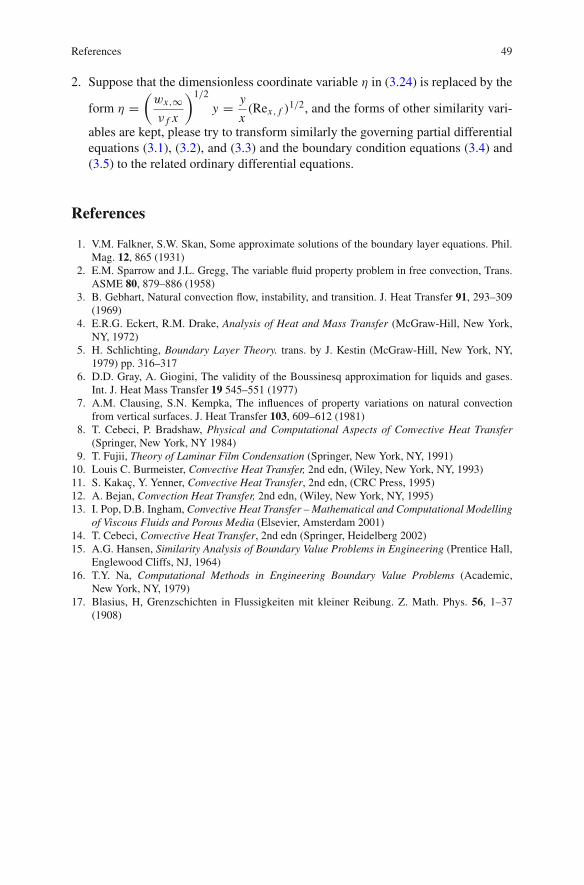
References 49
2. Suppose that the dimensionless coordinate variable η in (3.24) is replaced by the
form η =(wx,∞ν f x
)1/2
y = y
x(Rex, f )
1/2, and the forms of other similarity vari-
ables are kept, please try to transform similarly the governing partial differentialequations (3.1), (3.2), and (3.3) and the boundary condition equations (3.4) and(3.5) to the related ordinary differential equations.
References
1. V.M. Falkner, S.W. Skan, Some approximate solutions of the boundary layer equations. Phil.Mag. 12, 865 (1931)
2. E.M. Sparrow and J.L. Gregg, The variable fluid property problem in free convection, Trans.ASME 80, 879–886 (1958)
3. B. Gebhart, Natural convection flow, instability, and transition. J. Heat Transfer 91, 293–309(1969)
4. E.R.G. Eckert, R.M. Drake, Analysis of Heat and Mass Transfer (McGraw-Hill, New York,NY, 1972)
5. H. Schlichting, Boundary Layer Theory. trans. by J. Kestin (McGraw-Hill, New York, NY,1979) pp. 316–317
6. D.D. Gray, A. Giogini, The validity of the Boussinesq approximation for liquids and gases.Int. J. Heat Mass Transfer 19 545–551 (1977)
7. A.M. Clausing, S.N. Kempka, The influences of property variations on natural convectionfrom vertical surfaces. J. Heat Transfer 103, 609–612 (1981)
8. T. Cebeci, P. Bradshaw, Physical and Computational Aspects of Convective Heat Transfer(Springer, New York, NY 1984)
9. T. Fujii, Theory of Laminar Film Condensation (Springer, New York, NY, 1991)10. Louis C. Burmeister, Convective Heat Transfer, 2nd edn, (Wiley, New York, NY, 1993)11. S. Kakaç, Y. Yenner, Convective Heat Transfer, 2nd edn, (CRC Press, 1995)12. A. Bejan, Convection Heat Transfer, 2nd edn, (Wiley, New York, NY, 1995)13. I. Pop, D.B. Ingham, Convective Heat Transfer – Mathematical and Computational Modelling
of Viscous Fluids and Porous Media (Elsevier, Amsterdam 2001)14. T. Cebeci, Convective Heat Transfer, 2nd edn (Springer, Heidelberg 2002)15. A.G. Hansen, Similarity Analysis of Boundary Value Problems in Engineering (Prentice Hall,
Englewood Cliffs, NJ, 1964)16. T.Y. Na, Computational Methods in Engineering Boundary Value Problems (Academic,
New York, NY, 1979)17. Blasius, H, Grenzschichten in Flussigkeiten mit kleiner Reibung. Z. Math. Phys. 56, 1–37
(1908)

Chapter 4A New Similarity Analysis Method for LaminarForced Convection Boundary Layer
Abstract A new similarity analysis method with a new set of dimensionlesssimilarity variables is provided for complete similarity transformation of the gov-erning partial differential equations of laminar forced convection and two-phase filmflows. First, the derivation of the Reynolds number together with the Nusselt numberand Prandtl number is reviewed by means of Buckingham π -theorem and dimensionanalysis, where the Reynolds number is taken as the one of the new set of dimension-less analysis variables. Then the essential work focuses on derivation of equationsfor the dimensionless velocity components and the dimensionless coordinate vari-able, by means of a detailed analysis of quantity grade of the governing conservationpartial differential equations of laminar forced convection. On this basis, the newsimilarity analysis method is produced for complete similarity transformation ofthe conservation partial differential equations of laminar forced convection and itsfilm flows. Owing to dimensionless velocity components devoted in this chapter, thenew similarity analysis method has obvious advantages compared with the Falkner–Skan transformation. These advantages are the following: (i) more convenient forconsideration and treatment of the variable physical properties, (ii) more convenientfor analysis and investigation of the two-dimensional velocity field, and (iii) moreconvenient for satisfaction of the interfacial mass transfer matching conditions in thenumerical calculation and for rigorous investigation of mass transfer for two-phasefilm flows with three-point boundary problem. These advantages will be found fromthe successive chapters.
4.1 Introduction
In Chap. 3, we have briefly reviewed the Falkner-Skan type transformation. Up tonow, Falkner-Skan type transformation is a main approach applied for similarityanalysis and transformation of the governing partial differential equations of lam-inar forced convection and its two-phase film flows. With this method a streamfunction need to be induced, and then the dimensionless variable function f (η)and its derivatives are included in the transformed similarity mathematical model.It can be found that the disadvantages of the method are: (i) difficult for analysis
D.Y. Shang, Theory of Heat Transfer with Forced Convection Film Flows,Heat and Mass Transfer, DOI 10.1007/978-3-642-12581-2_4,C© Springer-Verlag Berlin Heidelberg 2011
51

52 4 A New Similarity Analysis Method
and investigation of the two-dimensional velocity field, (ii) difficult for satisfactionof the interfacial mass transfer matching conditions in the numerical calculation anddifficult for rigorous investigation of mass transfer for two-phase film flows withthree-point boundary problem, and (iii) difficult for consideration and treatment ofthe variable physical properties.
In [1], a new similarity analysis method was proposed on extensive investigationfor heat transfer of laminar free convection, and collected in [2]. Since then the seriesrelated studies have already proved that this new similarity method is better alter-native to the traditional Falkner-Skan type transformation for extensive studies onheat transfer of laminar free convection [3, 4], two-phase film flow boiling and con-densation [5–7], and falling film flow of non-Newtonian power-law fluids [8–10].In this chapter, a novel similarity analysis method will be reported for extensiveinvestigation of laminar forced convection and two-phase film condensation, forresolving the difficulties caused by the Falkner-Skan type transformation method.First, a system of dimensionless similarity variables, such as Reynolds num-ber, dimensionless coordinate variable, and dimensionless velocity components, isderived and determined through the analysis with the typical basis conservationequations on laminar forced convection. In derivation of the dimensionless simi-larity variables, it is never necessary to induce the stream function ψ, intermediatevariable f (η), and its derivatives. In this way, the above difficult points caused bythe Falkner-Skan type transformation can be overcome, which can be found in thesuccessive chapters of this book by using the present new similarity analysis methodfor extensive investigation of fluid forced convection and the two-phase forced filmcondensation.
4.2 Typical Basis Conservation Equations of LaminarForced Convection
For presentation of the present new similarity analysis method, (3.1), (3.2), and(3.3) are taken as the governing partial differential equations for laminar forced filmconvection boundary layer without consideration of variable physical properties andviscous thermal dissipation:
∂
∂x(wx)+ ∂
∂y(wy) = 0, (3.1)
wx∂wx
∂x+ wy
∂wx
∂y= ν f
∂2wx
∂y2 , (3.2)
wx∂t
∂x+ wy
∂t
∂y= ν f
Pr f
∂2t
∂y2, (3.3)
with the boundary condition equations
y = 0 : wx = 0, wy = 0, t = tw (3.4)
y → ∞ : wx = wx,∞(constant), t = t∞. (3.5)

4.3 Brief Review on Determination of Dimensionless Similarity Parameters (Number) 53
Here, the subscript “ f ” demonstrates that the value of the related physical prop-erty is taken at the boundary layer average temperature t f = tw+t∞
2 .Equations (3.1), (3.2), and (3.3) with the constant properties are now taken as
examples for presentation of the new similarity analysis method. First of all, it isnecessary to briefly review the determination on the dimensionless similarity param-eters for laminar forced convection.
4.3 Brief Review on Determination of Dimensionless SimilarityParameters (Number)
There are already three main dimensionless similarity parameters (number) for lam-inar forced convection, Nusselt number Nu, Reynolds number Re, and Prandtl num-ber Pr. The Nusselt number is used to express heat transfer at a boundary (surface)within a fluid; the Reynolds number gives a measure of the ratio of inertial forcesto viscous forces; and Pr is the ratio of momentum diffusivity (kinematic viscos-ity) and thermal diffusivity. Although only the Reynolds number is used for thesimilarity analysis and transformation of the governing partial differential equationsof laminar forced convection and film flows, the review for determination on allthese dimensionless similarity parameters will be presented here for fluid laminarforced convection. The popular method for creating the dimensionless similarityparameters is based on Buckingham π -theorem in dimensional analysis [11–21].Here, the π -theorem with dimension analysis is applied to derive the dimensionlesssimilarity parameters on laminar forced convection boundary layer.
With π -theorem, it is known that if a dependent physical phenomenon (variable)F0 is completely determined by a set of n independent variables, in which r basicdimensions are included, the suitable dependent principle F0 will be completelydetermined by n − r dimensionless similarity parameters. According to π -theorem,the derivation on the dimensionless similarity parameters is done successively asfollowing procedures.
4.3.1 Select Whole Physical Independent Variables Dominatingthe Physical Phenomenon
Observing governing equations (3.1), (3.2), and (3.3), it is seen that the whole phys-ical independent variables dominating the physical phenomenon of laminar forcedconvection boundary layer can be obtained and expressed as the following form:
F0(λ f , wx,∞, x, μ f , αx , ρ f , cp f ) = 0. (4.1)
Here, x is taken as the local length coordinate in the plate surface, the physicalproperties λ,μ, ρ, and cp are thermal conductivity, absolute viscosity, density, andspecific heat of the fluid, respectively, and α is heat transfer coefficient. While wx,∞
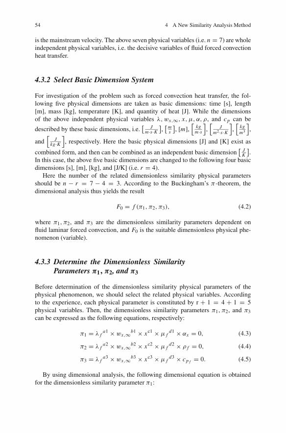
54 4 A New Similarity Analysis Method
is the mainstream velocity. The above seven physical variables (i.e. n = 7) are wholeindependent physical variables, i.e. the decisive variables of fluid forced convectionheat transfer.
4.3.2 Select Basic Dimension System
For investigation of the problem such as forced convection heat transfer, the fol-lowing five physical dimensions are taken as basic dimensions: time [s], length[m], mass [kg], temperature [K], and quantity of heat [J]. While the dimensionsof the above independent physical variables λ,wx,∞, x, μ, α, ρ, and cp can be
described by these basic dimensions, i.e.[ J
m·s·K],[m
s
], [m],
[kgm·s],[
Jm2·s·K
],[
kgm3
],
and[
Jkg·K], respectively. Here the basic physical dimensions [J] and [K] exist as
combined form, and then can be combined as an independent basic dimension[ J
K
].
In this case, the above five basic dimensions are changed to the following four basicdimensions [s], [m], [kg], and [J/K] (i.e. r = 4).
Here the number of the related dimensionless similarity physical parametersshould be n − r = 7 − 4 = 3. According to the Buckingham’s π -theorem, thedimensional analysis thus yields the result
F0 = f (π1, π2, π3), (4.2)
where π1, π2, and π3 are the dimensionless similarity parameters dependent onfluid laminar forced convection, and F0 is the suitable dimensionless physical phe-nomenon (variable).
4.3.3 Determine the Dimensionless SimilarityParameters π1, π2, and π3
Before determination of the dimensionless similarity physical parameters of thephysical phenomenon, we should select the related physical variables. Accordingto the experience, each physical parameter is constituted by r + 1 = 4 + 1 = 5physical variables. Then, the dimensionless similarity parameters π1, π2, and π3can be expressed as the following equations, respectively:
π1 = λ fa1 × wx,∞b1 × xc1 × μ f
d1 × αx = 0, (4.3)
π2 = λ fa2 × wx,∞b2 × xc2 × μ f
d2 × ρ f = 0, (4.4)
π3 = λ fa3 × wx,∞b3 × xc3 × μ f
d3 × cp f = 0. (4.5)
By using dimensional analysis, the following dimensional equation is obtainedfor the dimensionless similarity parameter π1:

4.3 Brief Review on Determination of Dimensionless Similarity Parameters (Number) 55
[J
s · K · m
]a1
·[m
s
]b1 · [m]c1 ·[
kg
m · s
]d1
·[
J
s · K · m2
]= 0.
Obviously, the indexes a1 to d1 are suitable to the following equations:
For dimension [kg] balance: d1 = 0For dimension [m] balance: −a1 + b1 + c1 − d1 − 2 = 0For dimension [s] balance: −a1 − b1 − d1 − 1 = 0For dimension [J/K]: a1 + 1 = 0The solutions are a1 = −1, b1 = 0, c1 = 1, d1 = 0
Then the dimensionless similarity parameter π1 is
π1 = αx x
λ f.
It is the well-known local Nusselt number without consideration of thermophysicalphysical properties, i.e.
Nux, f = αx x
λ f, (4.6)
where λ f is the average thermal conductivity at the boundary layer averagetemperature
t f = tw + t∞2
.
By using dimensional analysis, the following dimensional equation is obtainedfor the dimensionless similarity parameter π2:
[J
s · K · m
]a2
·[m
s
]b2 · [m]c2 ·[
kg
m · s
]d2
·[
kg
m3
]= 0.
Obviously, the indexes a2 to d2 are suitable to the following equations:
For dimension [kg] balance: d2 + 1 = 0For dimension [m] balance: −a2 + b2 + c2 − d2 − 3 = 0For dimension [s] balance: −a2 − b2 − d2 = 0For dimension [J/K]: a2 = 0The solutions are a2 = 0, b2 = 1, c2 = 1, d2 = −1.
Then, we can obtain a following dimensionless parameter:
π2 = wx,∞xρ f
μ for π2 = wx,∞x
ν f.

56 4 A New Similarity Analysis Method
This is the well-known local Reynolds number without consideration of variablethermophysical properties, i.e.
Rex, f = wx,∞x
ν f. (4.7)
By using dimensional analysis, the following dimensional equation is obtained forthe dimensionless similarity parameter π3:
[J
s · K · m
]a3
·[m
s
]b3 · [m]c3 ·[
kg
m · s
]d3
·[
J
kg · K
]= 0.
Obviously, the indexes a3 to d3 are suitable to the following equations:
For dimension [kg] balance: d3 − 1 = 0For dimension [m] balance: −a3 + b3 + c3 − d3 = 0For dimension [s] balance: −a3 − b3 − d3 = 0For dimension [J/K]: a3 + 1 = 0The solutions are a3 = −1, b3 = 0, c3 = 0, d3 = 1.
Then
π3 = μ f · cp f
λ f.
This is the average Prandtl number Prf, i.e.
Pr f = μ f · cp f
λ f. (4.8)
So far, we have reviewed the derivation for obtaining thee dimensionless similarityparameters, Nusselt number, Reynolds number, and Prandtl number, respectively,for fluid laminar forced convection. On this basis, in the following section, we fur-ther investigate the dimensionless similarity variables related to the velocity field,which is the focal point of this chapter.
4.4 Investigation of the Dimensionless Similarity Variableson the Velocity Field
Here, with the basic momentum conservation equation, an analysis method will beapplied for investigation of the dimensionless similarity variables on the velocityfield of laminar forced convection boundary layer.
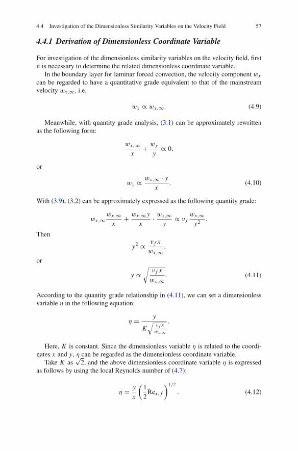
4.4 Investigation of the Dimensionless Similarity Variables on the Velocity Field 57
4.4.1 Derivation of Dimensionless Coordinate Variable
For investigation of the dimensionless similarity variables on the velocity field, firstit is necessary to determine the related dimensionless coordinate variable.
In the boundary layer for laminar forced convection, the velocity component wx
can be regarded to have a quantitative grade equivalent to that of the mainstreamvelocity wx,∞, i.e.
wx ∝ wx,∞. (4.9)
Meanwhile, with quantity grade analysis, (3.1) can be approximately rewrittenas the following form:
wx,∞x
+ wy
y∝ 0,
or
wy ∝ wx,∞ · y
x. (4.10)
With (3.9), (3.2) can be approximately expressed as the following quantity grade:
wx,∞wx,∞
x+ wx,∞y
x· wx,∞
y∝ ν f
wx,∞y2 .
Then
y2 ∝ ν f x
wx,∞,
or
y ∝√ν f x
wx,∞. (4.11)
According to the quantity grade relationship in (4.11), we can set a dimensionlessvariable η in the following equation:
η = y
K√
ν f xwx,∞
.
Here, K is constant. Since the dimensionless variable η is related to the coordi-nates x and y, η can be regarded as the dimensionless coordinate variable.
Take K as√
2, and the above dimensionless coordinate variable η is expressedas follows by using the local Reynolds number of (4.7):
η = y
x
(1
2Rex, f
)1/2
. (4.12)

58 4 A New Similarity Analysis Method
4.4.2 Derivation for Dimensionless Velocity Components
After determination of the expression of the dimensionless coordinate variable η,the investigation focuses on creation of the appropriate forms of the dimensionlessvelocity components. For this purpose, first, set Wx (η) as the dimensionless veloc-ity component in x coordinate and suppose the velocity component wx is directlyproportional to Wx (η), mainstream velocity wx,∞, and the pth power of the localReynolds number, i.e. (Rex, f )
p. Additionally, set Wy(η) as the dimensionless veloc-ity component in y coordinate and suppose the velocity component wy is directlyproportional to Wy(η), the mainstream velocity wx,∞ and qth power of the localReynolds number, i.e. (Rex, f )
q . Then, we have the following supposed equationsabout the two-dimensional velocity components wx and wy , respectively:
wx = wx,∞(
1
2Rex, f
)p
· Wx (η), (4.13)
wy = wx,∞(
1
2Rex, f
)q
Wy(η). (4.14)
From (4.12) with (4.7), we have
∂η
∂x= −1
2x−3/2 y
(1
2
wx,∞ν f
)1/2
,
= −1
2x−2 y
(1
2
wx,∞ · x
ν f
)1/2
, (4.15)
= −1
2x−1η.
∂η
∂y= 1
x
(1
2Rex
)1/2
. (4.16)
The partial derivative ∂wx∂x is expressed as
∂wx
∂x= wx,∞ · p
(1
2Rex, f
)p−1(
1
2
wx,∞ν f
)· Wx (η)
+ wx,∞(
1
2Rex, f
)p dWx (η)
dη· ∂η∂x,
= x−1wx,∞ · p
(1
2
wx,∞x
ν f
)p−1(1
2
wx,∞x
ν f
)·Wx (η)
+ wx,∞(
1
2Rex, f
)p dWx (η)
dη· ∂η∂x,

4.4 Investigation of the Dimensionless Similarity Variables on the Velocity Field 59
= px p−1wx,∞
(1
2
wx,∞ν f
)p
· Wx (η)+ wx,∞(
1
2Rex, f
)p dWx (η)
dη· ∂η∂x,
= px−1wx,∞(
1
2Rex, f
)p
· Wx (η)+ wx,∞(
1
2Rex, f
)p dWx (η)
dη· ∂η∂x.
With (4.15), the above equation becomes
∂wx
∂x= px−1wx,∞
(1
2Rex, f
)p
· Wx (η)+ wx,∞(
1
2Rex, f
)p
· dWx (η)
dη
(−1
2x−1η
),
= x−1(
1
2Rex, f
)p
· wx,∞[
p · Wx (η)− 1
2η
dWx (η)
dη
]. (4.17)
With (4.14) we have
∂wx
∂y=(
1
2Rex, f
)p
wx,∞dWx (η)
dη· ∂η∂y.
With (4.16) the above equation becomes
∂wx
∂y=(
1
2Rex, f
)p
wx,∞dWx (η)
dη· 1
x
(1
2Rex, f
)1/2
, (4.18)
= 1
x
(1
2Rex, f
)p+1/2
wx,∞dWx (η)
dη.
Also
∂2wx
∂y2 = 1
x
(1
2Rex, f
)p+1/2
wx,∞d2Wx (η)
dη2 · ∂η∂y,
= 1
x
(1
2Rex, f
)p+1/2
wx,∞d2Wx (η)
dη2· 1
x
(1
2Rex, f
)1/2
, (4.19)
= 1
x2
(1
2Rex, f
)p+1
wx,∞d2Wx (η)
dη2 .
Then (3.2) is transformed to

60 4 A New Similarity Analysis Method
wx,∞(
1
2Rex, f
)p
· Wx (η) · x−1(
1
2Rex, f
)p
wx,∞[
p · Wx (η)− 1
2η
dWx (η)
dη
]
+ wx,∞(
1
2Rex, f
)q
· Wy(η) · 1
x
(1
2Rex, f
)p+1/2
wx,∞dWx (η)
dη
= ν f1
x2
(1
2Rex, f
)p+1
wx,∞d2Wx (η)
dη2.
The above equation is rewritten as
wx,∞(
1
2Rex, f
)p
· Wx (η) · x−1(
1
2Rex, f
)p
wx,∞[
p · Wx (η)− 1
2η
dWx (η)
dη
]
+ wx,∞(
1
2Rex, f
)q
· Wy(η)1
x
(1
2Rex, f
)p+1/2
wx,∞dWx (η)
dη
= ν f
wx,∞ · x· 1
x
(1
2Rex, f
)p+1
· wx,∞2 · d2Wx (η)
dη2.
i.e.
wx,∞(
1
2Rex, f
)p
· Wx (η) · x−1(
1
2Rex, f
)p
wx,∞[
pWx (η)− 1
2η
dWx (η)
dη
]
+ wx,∞(
1
2Rex, f
)q
· Wy(η) · 1
x
(1
2Rex, f
)p+1/2
wx,∞dWx (η)
dη
= 1
2x
(1
2Rex, f
)p
wx,∞2 d2Wx (η)
dη2.
The above equation is divided by 1x
(12 Rex, f
)2p · wx,∞2 and simplified to
Wx (η) ·[
p · Wx (η)− 1
2η
dWx (η)
dη
]+ Wy(η) ·
(1
2Rex, f
)−p+q+1/2 dWx (η)
dη
=(
1
2
)(1
2Rex, f
)−p d2Wx (η)
dη2 (4.20)
If (4.20) becomes a complete similarity dimensionless equations, obviously weshould have

4.4 Investigation of the Dimensionless Similarity Variables on the Velocity Field 61
−p + q + 1
2= 0. (4.21)
−p = 0. (4.22)
Then, p = 0 and q = − 12 .
Then the supposed equations (4.13) and (4.14) for the two-dimensionalvelocity components of laminar forced boundary layer are expressed as,respectively,
wx = wx,∞ · Wx (η), (4.23)
wy = wx,∞ ·(
1
2Rex, f
)−1/2
· Wy(η), (4.24)
or
Wx (η) = wx
wx,∞, (4.23a)
Wy(η) = wy
wx,∞
(1
2Rex, f
)1/2
. (4.24a)
These are expressions for the new similarity velocity components Wx (η) and Wy(η)
derived by using the new similarity analysis method for laminar forced convectionboundary layer.
The related expressions on the two-dimensional velocity components wx and wy
based on the Falkner-Skan transformation are
wx = wx,∞ f ′(η), (3.28)
wy = 1
2wx,∞
(1
2Rex, f
)−1/2
[η · f ′(η)− f (η)]. (3.30)
Comparing (3.28) and (3.30) with (4.23) and (4.24), respectively, we can obtainthe following equations for relationship of the new similarity velocity componentsWx (η) and Wy(η) with the dimensionless function f (η):
Wx (η) = f ′(η), (4.25)
Wy(η) =(
1
2
) [η f ′(η)− f (η)
]. (4.26)
From (4.23), (4.24), (4.25), and (4.26), the following points can be concluded fromcomparison of the dimensionless similarity variables Wx (η) and Wy(η) with thedimensionless function f (η) on the momentum velocity field: The derived dimen-sionless similarity velocity components Wx (η) and Wy(η) based on the present new

62 4 A New Similarity Analysis Method
similarity analysis method are directly proportional to the related velocity compo-nents wx and wy , while the relationships of dimensionless function f (η) based onthe Falkner-Skan type transformation with the velocity components wx and wy aremore complicated, and even complicated issue caused by (3.30), which expresses amore complicated relationship between f (η) and wy .
On contrary, the simpler relationships of the dimensionless similarity variablesWx (η) and Wy(η) with the related velocity component wx and wy lead to two fol-lowing advantages for the dimensionless governing equations derived by the newsimilarity analysis method compared with those by the Falkner-Skan type trans-formation: (i) more convenient to consider and treat the variable thermophysicalproperties, and (ii) more convenient to treat and satisfy the interfacial matching con-ditions for further rigorous investigation of heat and mass transfer of laminar forcedfilm condensation. In the following chapters, these advantages with the present newsimilarity analysis method can be found successively.
Additionally, for dimensionless similarity analysis and transformation of the gov-erning energy partial differential equation of fluid laminar forced convection, (3.3),we take the well-known form of the dimensionless temperature variable θ(η) as
θ(η) = t − t∞tw − t∞
. (4.27)
Up to now, the whole set of equations for the dimensionless similarity analysis vari-ables, i.e. the local Reynolds number Rex, f , dimensionless similarity variables η,dimensionless velocity components Wx (η) and Wy(η), and dimensionless temper-ature θ , based on the new similarity analysis method can be collected below for aclear expression:
Rex, f = wx,∞x
ν f, (4.7)
η = y
x
(1
2Rex, f
)1/2
, (4.12)
wx = wx,∞ · Wx (η), (4.23)
wy = wx,∞ ·(
1
2Rex, f
)−1/2
· Wy(η), (4.24)
θ(η) = t − t∞tw − t∞
. (4.27)
Comparing the above set of similarity dimensionless variable for the new simi-larity analysis method with those in (3.24), (3.25), (3.28), (3.30), and (3.31) forthe Falkner-Skan type transformation, it is found that their differences are in thedimensionless similarity variables related to the velocity field. However, in the nextsection, we will find that these differences will lead to quite different similarity

4.5 Application Example of the New Similarity Analysis Method 63
dimensionless equations for laminar forced convection boundary layer based on thepresent new similarity analysis method from those based on the Falkner-Skan typetransformation.
4.5 Application Example of the New Similarity Analysis Method
In this section, the expressions (4.7), (4.12), (4.23), (4.24), and (4.27), respectively,for the new system of similarity variables Rex, f , η, Wx , Wy , and θ based on the newsimilarity analysis method will be applied for complete similarity transformation ofthe governing partial differential equations (3.1) (3.2) and (3.3) with their boundarycondition equations (3.4) and (3.5) of laminar forced convection boundary layer forignoring constant properties.
4.5.1 Similarity Transformation of (3.1)
With (4.12) and (4.23), we have
∂wx
∂x= wx,∞
dWx (η)
dη· ∂η∂x.
Where with (4.7), we have
∂η
∂x= −1
2x−3/2 y
(1
2
wx,∞ν f
)1/2
= −1
2x−2 y
(1
2
wx,∞ · x
ν f
)1/2
. (4.28)
= −1
2x−1η
Then
∂wx
∂x= −1
2x−1η · wx,∞
dWx (η)
dη. (4.29)
With (4.24) we have
∂wy
∂y= wx,∞
(1
2Rex, f
)−1/2 dWy(η)
dη· ∂η∂y.
Where according to (4.12)

64 4 A New Similarity Analysis Method
∂η
∂y= x−1
(1
2Rex, f
)1/2
. (4.30)
Then
∂wy
∂y= wx,∞
(1
2Rex, f
)−1/2 dWy(η)
dηx−1(
1
2Rex, f
)1/2
. (4.31)
= x−1wx,∞dWy(η)
dη
Then (3.1) is changed to
−1
2x−1η · wx,∞
dWx (η)
dη+ x−1wx,∞
dWy(η)
dη= 0.
The above equation is simplified to
− ηdWx (η)
dη+ 2
dWy(η)
dη= 0. (4.32)
4.5.2 Similarity Transformation of (3.2)
With (4.12) and (4.23) we have
∂wx
∂y= wx,∞
dWx (η)
dη· ∂η∂y.
With (4.12) we have
∂η
∂y= x−1
(1
2Rex, f
)1/2
. (4.33)
Then
∂wx
∂y= x−1
(1
2Rex, f
)1/2
wx,∞dWx (η)
dη, (4.34)
∂2wx
∂y2 = x−1(
1
2Rex, f
)1/2
wx,∞d2Wx (η)
dη2 · dη
dy
= x−1(
1
2Rex, f
)1/2
wx,∞d2Wx (η)
dη2 x−1(
1
2Rex, f
)1/2
. (4.35)
= x−2(
1
2Rex, f
)· wx,∞
d2Wx (η)
dη2

4.5 Application Example of the New Similarity Analysis Method 65
Then (3.2) is changed to
− 1
2wx,∞Wx (η) · x−1η · wx,∞
dWx (η)
dη+ wx,∞
(1
2Rex, f
)−1/2
Wy(η) · x−1(
1
2Rex, f
)1/2
wx,∞dWx (η)
dη
= ν f · x−2(
1
2Rex, f
)· wx,∞
d2Wx (η)
dη2.
The above equation is simplified to
−1
2wx,∞Wx (η) · x−1η · wx,∞
dWx (η)
dη+ wx,∞ · Wy(η) · x−1 · wx,∞
dWx (η)
dη
= ν f · x−2(
1
2
wx,∞x
ν f
)· wx,∞
d2Wx (η)
dη2.
The above equation is divided by 12 x−1 · wx,∞2, and simplified to
[−η · Wx (η)+ 2Wy(η)]dWx (η)
dη= d2Wx (η)
dη2 . (4.36)
4.5.3 Similarity Transformation of (3.3)
With (4.27), we have
∂t
∂x= (tw − t∞)
dθ(η)
dη· ∂η∂x.
With (4.28), the above equation is expressed as
∂t
∂x= −1
2x−1η(tw − t∞)
dθ(η)
dη(4.37)
With (4.27), we have
∂t
∂y= (tw − t∞)
dθ(η)
dη· ∂η∂y

66 4 A New Similarity Analysis Method
With (4.33), the above equation is expressed as
∂t
∂y= (tw − t∞)
dθ(η)
dηx−1(
1
2Rex, f
)1/2
, (4.38)
∂2t
∂y2= (tw − t∞)x−1
(1
2Rex, f
)1/2 d2θ(η)
dη2· ∂η∂y, (4.39)
= (tw − t∞)x−1(
1
2Rex, f
)1/2 d2θ(η)
dη2· x−1
(1
2Rex, f
)1/2
,
= 1
2(tw − t∞)x−2Rex, f
d2θ(η)
dη2 .
Then (3.3) is changed to
wx,∞W (η)x ·[−1
2x−1η · (tw − t∞)
dθ(η)
dη
]+ wx,∞
(1
2Rex, f
)−1/2
Wy(η) · (tw − t∞)dθ(η)
dηx−1(
1
2Rex, f
)1/2
= ν f
Pr f
1
2(tw − t∞)x−2Rex, f
d2θ(η)
dη2 .
i.e.
−1
2wx,∞Wx (η) · x−1η · (tw − t∞)
dθ(η)
dη+ wx,∞Wy(η) · (tw − t∞)
dθ(η)
dηx−1
= 1
2
ν f
Pr f(tw − t∞)x−2Rex, f
d2θ(η)
dη2
.
With the definition of Rex, f in (4.7), the above equation is further simplified to
−1
2wx,∞Wx (η) · x−1η · (tw − t∞)
dθ(η)
dη+ wx,∞Wy(η)(tw − t∞)
dθ(η)
dηx−1
= 1
2
ν f
Pr f(tw − t∞)x−2wx,∞x
ν f
d2θ(η)
dη2
.
The above equation is divided by 12 x−1wx,∞(tw − t∞), and simplified to
−Wx (η) · ηdθ(θ)
dη+ 2Wy(η) · dθ(η)
dη= 1
Pr f
d2θ(η)
dη2,
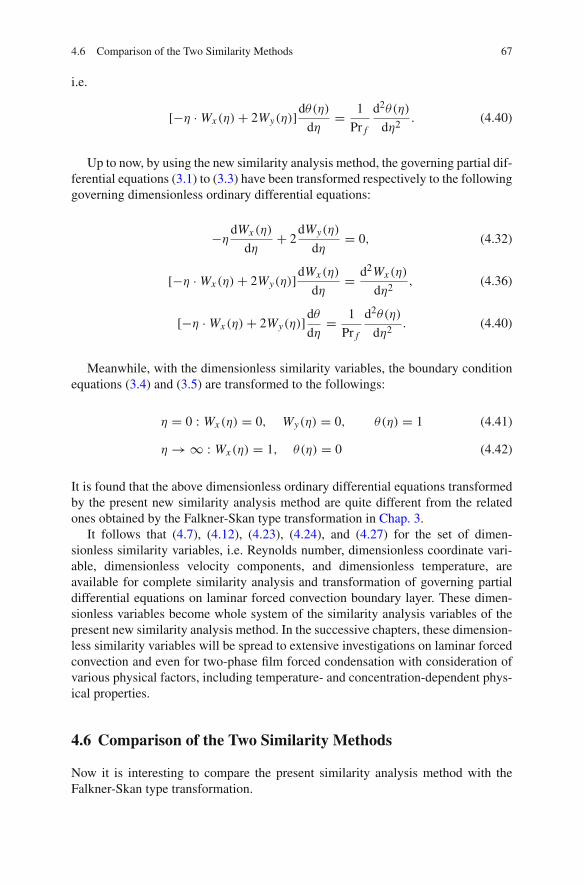
4.6 Comparison of the Two Similarity Methods 67
i.e.
[−η · Wx (η)+ 2Wy(η)]dθ(η)
dη= 1
Pr f
d2θ(η)
dη2. (4.40)
Up to now, by using the new similarity analysis method, the governing partial dif-ferential equations (3.1) to (3.3) have been transformed respectively to the followinggoverning dimensionless ordinary differential equations:
−ηdWx (η)
dη+ 2
dWy(η)
dη= 0, (4.32)
[−η · Wx (η)+ 2Wy(η)]dWx (η)
dη= d2Wx (η)
dη2, (4.36)
[−η · Wx (η)+ 2Wy(η)]dθ
dη= 1
Pr f
d2θ(η)
dη2 . (4.40)
Meanwhile, with the dimensionless similarity variables, the boundary conditionequations (3.4) and (3.5) are transformed to the followings:
η = 0 : Wx (η) = 0, Wy(η) = 0, θ(η) = 1 (4.41)
η → ∞ : Wx (η) = 1, θ(η) = 0 (4.42)
It is found that the above dimensionless ordinary differential equations transformedby the present new similarity analysis method are quite different from the relatedones obtained by the Falkner-Skan type transformation in Chap. 3.
It follows that (4.7), (4.12), (4.23), (4.24), and (4.27) for the set of dimen-sionless similarity variables, i.e. Reynolds number, dimensionless coordinate vari-able, dimensionless velocity components, and dimensionless temperature, areavailable for complete similarity analysis and transformation of governing partialdifferential equations on laminar forced convection boundary layer. These dimen-sionless variables become whole system of the similarity analysis variables of thepresent new similarity analysis method. In the successive chapters, these dimension-less similarity variables will be spread to extensive investigations on laminar forcedconvection and even for two-phase film forced condensation with consideration ofvarious physical factors, including temperature- and concentration-dependent phys-ical properties.
4.6 Comparison of the Two Similarity Methods
Now it is interesting to compare the present similarity analysis method with theFalkner-Skan type transformation.

68 4 A New Similarity Analysis Method
4.6.1 Different Derivation Process of the Dimensionless SimilarityVariables on Momentum Field
The dimensionless similarity variables on momentum field corresponding to theFalkner-Skan type transformation were derived by the group theory. In the deriva-tion, the stream function was induced, and dimensionless function f (η) was takenas the intermediate variable related to two-dimensional velocity components. Suchderivation process is corresponding to a more complicated procedure.
The dimensionless similarity variables on momentum field corresponding tothe present similarity analysis method are derived by the analysis on the basicmass and momentum conservation equations of laminar forced convection boundarylayer. First, the appropriate dimensionless models for the two-dimensional similarityvelocity components are respectively supposed to be a product of the related veloc-ity component, mainstream velocity, and a power of local Reynolds number. Thendetermination of the exponent of local Reynolds number becomes the key work. Itis seen that such derivation processes of the appropriate relations are distinct andclear by using the present similarity analysis method.
4.6.2 Different Dimensionless Expressions on Momentum Field
By comparing the dimensionless similarity variables in (3.35) and (3.39) derivedby the Falkner-Skan type transformation with those in (4.32), (4.36), and (4.40)obtained by the present similarity analysis method, it is found that their differenceis in the expressions of the similarity momentum field. The latter dimensionlesssimilarity variables on the momentum field are dimensionless velocity components,proportional directly to the mainstream velocity and related velocity component forx and y coordinates, and also a power of the Reynolds number. But the formerdimensionless similarity variables on the momentum field have more complicatedform with the velocity component wy . Such more complicated form on the velocitycomponent wy related to the dimensionless similarity variable on momentum fieldbased on the Falkner-Skan type transformation will hinder a series of extensiveinvestigations of laminar forced convection and two-phase film forced condensa-tion, such as for consideration of momentum field, variable physical properties,two-phase film flow interfacial matching conditions, and condensate mass transfer,and so on.
4.6.3 Different Similarity Analysis GoverningMathematical Models
The quite different dimensionless similarity variables on momentum fields basedon the Falkner-Skan type transformation and the present similarity analysis methodlead to quite different dimensionless similarity governing mathematical models. Thesimilarity governing mathematical model based on the Falkner-Skan transformation

4.7 Remarks 69
causes a difficulty for clarifying the two-dimensional flow velocity field, for consid-eration of variable physical properties, and even for further investigating heat andmass transfer of two-phase film condensation. It will be found in the successivechapters that the dimensionless similarity governing mathematical model based onthe present similarity analysis method can resolve the above shortages caused bythe traditional Falkner-Skan transformation, can be suitable for broad respects ofresearch on laminar forced convection and two-phase film condensation, such asthat with consideration and treatment of concentration and temperature-dependentphysical properties, for dealing with the interfacial physical matching conditions,and for deep investigation of heat and mass transfer.
4.7 Remarks
In this chapter, a new similarity analysis method is reported with a detailed deriva-tion for similarity analysis and transformation of laminar forced convection andtwo-phase film flows. A system of dimensionless similarity variables are providedincluding the dimensionless coordinate variable η, local Reynolds number Rex, f ,dimensionless velocity components Wx (η) and Wy(η), and dimensionless tempera-ture variable θ(η) for complete similarity analysis and transformation of a system ofgoverning partial differential equations of laminar forced convection. In particular,the expressions of the similarity variables, i.e. dimensionless velocity componentsdevoted in this book, have special advantages over those of the Falkner–Skan-typetransformation for resolving the challenges of extensive investigations of laminarforced convection and its film condensation. These advantages can be found in suc-cessive chapters.
First, the derivation of the Reynolds number together with the Nusselt numberand Prandtl number is reviewed by means of π -theorem for dimension analysis,where the local Reynolds number is useful in determination of the dimensionlesssimilarity variables. The next work focuses on derivation of the dimensionless sim-ilarity variables on the momentum field by means of a series of special analyseson the governing partial differential equations. These derived similarity variableson the momentum field are dimensionless coordinate variable η and dimensionlessvelocity components Wx (η) and Wy(η). On this basis, the system of the dimension-less similarity variables is proposed for the similarity analysis and transformation ofthe governing partial differential equations on laminar forced convection. Finally,by means of the system of provided equations with the dimensionless similarityvariables, the typical partial differential equations on laminar forced convection arecompletely transformed to the related dimensionless differential equations. It veri-fied that the provided system of the dimensionless similarity variables are availablefor the complete similarity analysis and transformation of the governing partial dif-ferential equations of the laminar forced convection, and the present new similarityanalysis method is valid.
The biggest difference of the present similarity analysis method from the Falkner-Skan type transformation is in their dimensionless similarity variables on the
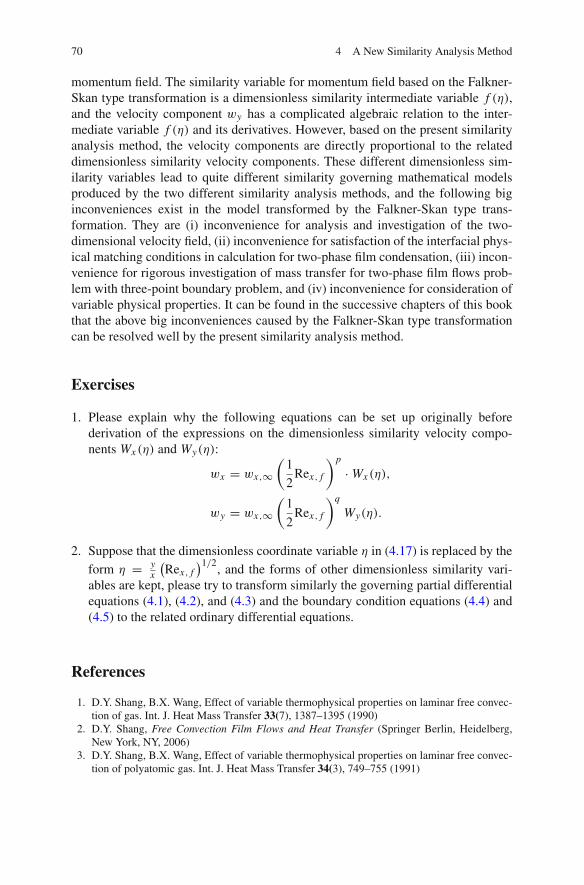
70 4 A New Similarity Analysis Method
momentum field. The similarity variable for momentum field based on the Falkner-Skan type transformation is a dimensionless similarity intermediate variable f (η),and the velocity component wy has a complicated algebraic relation to the inter-mediate variable f (η) and its derivatives. However, based on the present similarityanalysis method, the velocity components are directly proportional to the relateddimensionless similarity velocity components. These different dimensionless sim-ilarity variables lead to quite different similarity governing mathematical modelsproduced by the two different similarity analysis methods, and the following biginconveniences exist in the model transformed by the Falkner-Skan type trans-formation. They are (i) inconvenience for analysis and investigation of the two-dimensional velocity field, (ii) inconvenience for satisfaction of the interfacial phys-ical matching conditions in calculation for two-phase film condensation, (iii) incon-venience for rigorous investigation of mass transfer for two-phase film flows prob-lem with three-point boundary problem, and (iv) inconvenience for consideration ofvariable physical properties. It can be found in the successive chapters of this bookthat the above big inconveniences caused by the Falkner-Skan type transformationcan be resolved well by the present similarity analysis method.
Exercises
1. Please explain why the following equations can be set up originally beforederivation of the expressions on the dimensionless similarity velocity compo-nents Wx (η) and Wy(η):
wx = wx,∞(
1
2Rex, f
)p
· Wx (η),
wy = wx,∞(
1
2Rex, f
)q
Wy(η).
2. Suppose that the dimensionless coordinate variable η in (4.17) is replaced by theform η = y
x
(Rex, f
)1/2, and the forms of other dimensionless similarity vari-
ables are kept, please try to transform similarly the governing partial differentialequations (4.1), (4.2), and (4.3) and the boundary condition equations (4.4) and(4.5) to the related ordinary differential equations.
References
1. D.Y. Shang, B.X. Wang, Effect of variable thermophysical properties on laminar free convec-tion of gas. Int. J. Heat Mass Transfer 33(7), 1387–1395 (1990)
2. D.Y. Shang, Free Convection Film Flows and Heat Transfer (Springer Berlin, Heidelberg,New York, NY, 2006)
3. D.Y. Shang, B.X. Wang, Effect of variable thermophysical properties on laminar free convec-tion of polyatomic gas. Int. J. Heat Mass Transfer 34(3), 749–755 (1991)

References 71
4. Shang, B.X. Wang, Y. Wang, Y. Quan, Study on liquid laminar free convection with consid-eration of variable thermophysical properties. Int. J. Heat Mass Transfer 36(14), 3411–3419(1993)
5. D.Y. Shang , B.X. Wang, L.C. Zhong, A study on laminar film boiling of Liquid along anisothermal vertical plate in a pool with consideration of variable thermophysical properties.Int. J. Heat Mass Transfer 37(5), 819–828 (1994)
6. D.Y. Shang, T. Adamek, Study on laminar film condensation of saturated steam on a verti-cal flat plate for consideration of various physical factors including variable thermophysicalproperties. Wärme- und Stoffübertragung 30, 89–100 (1994)
7. D.Y. Shang, B.X. Wang, An extended study on steady-state laminar film condensation of asuperheated vapor on an isothermal vertical plate. Int. J. Heat Mass Transfer 40(4), 931–941(1997)
8. H.I. Andersson, D.Y. Shang, An extended study of hydrodynamics of gravity- driven film flowof power-law fluids. Fluid Dyn Res 22, 345–357 (1998)
9. D.Y. Shang, H. Andersson, Heat transfer in gravity-driven film flow of power-law fluids. Int.J. Heat Mass Transfer 42(11), 2085–2099 (1999)
10. D.Y. Shang, J. Gu, Analyses of pseudo-similarity and boundary layer thickness for non-Newtonian falling film flow. Heat Mass Transfer 41(1), 44–50, (2004)
11. E. Buckingham, On physically similar systems; illustrations of the use of dimensional equa-tions. Phys. Rev. 4, 345–376 (1914)
12. E. Buckingham, The principle of similitude. Nature 96, 396–397 (1915)13. E. Buckingham, Model experiments and the forms of empirical equations. Trans. A.S.M.E 37,
263–296 (1915)14. S.G. Taylor, The formation of a blast wave by a very intense explosion I. theoretical discussion.
Proc. Roy. Soc. A 201, 159–174 (1950)15. S.G. Taylor, The formation of a blast wave by a very intense explosion II. the atomic explosion
of 1945. Proc. Roy. Soc. A 201, 175–186 (1950)16. H. Hanche-Olsen, Buckingham’s pi-theorem, TMA4195 Mathematical modelling, NTNU
(2004)17. S J. Kline Similitude and Approximation Theory (Springer, New York, NY, 1986)18. F. Y.M. Wan, Mathematical Models and their Analysis (Harper & Row Publishers, New York,
NY, 1989)19. G.W. Hart Multidimensional Analysis: Algebras and Systems for Science and Engineering
(Springer, Heidelberg, 1995)20. Vignaux, G.A., Dimensional analysis in data modelling, Victoria University of Wellington,
1991. Retrieved December 15 (2005)21. Mike Sheppard, Systematic Search for Expressions of Dimensionless Constants using the
NIST database of Physical Constants (2007)

Part IILaminar Forced Convection

Chapter 5Heat Transfer on Laminar Forced Convectionwith Ignoring Variable Physical Propertiesand Viscous Thermal Dissipation
Abstract The present new similarity analysis method is applied for similarity trans-formation of governing partial differential equations for laminar forced convectionwithout consideration of variable physical properties and viscous thermal dissi-pation, and then the complete similarity mathematical model is obtained. In thetransformed dimensionless equations, dimensionless similarity velocity componentsWx (η) and Wy(η) describe clearly the forced convection momentum field. The rigor-ous numerical solutions on velocity and temperature fields, as well as heat transferequations, are obtained, which are very well coincident to Blasius and Pohlhausensolutions. All these prove that the present new similarity analysis method isvalid.
5.1 Introduction
Blasius [1] described the two-dimensional boundary layer of laminar forced convec-tion on a semi-infinite plate parallel to a main constant flow wx,∞. He transformedthe partial differential equations related to the momentum field to a single ordinarydifferential equation by transforming the coordinate system. Then, the Blasius trans-formation approach was generalised by Falkner-Skan type transformation [2] forouter flows of the form = cxm results, and then the Falkner-Skan type transforma-tion has had widespread application and widely collected in numerous books, suchas [3–11] for laminar forced convection with boundary layer analysis. However, theFalkner-Skan type transformation has some disadvantages, which will cause diffi-culties for consideration of variable physical properties, and for treatment of thetwo-phase film flow interfacial physical matching conditions. The latter advantagewill further lead to a difficulty for reliable investigation of two-phase flow conden-sation heat and mass transfer. In order to overcome these disadvantages, the newsimilarity analysis method was presented in detail in Chap. 4. From this chapteronwards, this new similarity analysis method will be successively used in extensiveinvestigation on the laminar forced convection and two-phase film condensation.First, in this chapter, a typical case on laminar forced convection will be touched forignoring variable physical properties and viscous thermal dissipation.
D.Y. Shang, Theory of Heat Transfer with Forced Convection Film Flows,Heat and Mass Transfer, DOI 10.1007/978-3-642-12581-2_5,C© Springer-Verlag Berlin Heidelberg 2011
75
76 5 Heat Transfer on Laminar Forced Convection
5.2 Basic Conservation Equations of Laminar Forced Convection
5.2.1 Governing Partial Differential Equations
In Fig. 5.1 the physical model and coordinate system of boundary layer with two-dimensional laminar forced convection are shown schematically. A flat plate is hor-izontally located in parallel fluid flow with its mainstream velocity wx,∞. The platesurface temperature is tw and the fluid bulk temperature is t∞. Then, a velocityboundary layer is produced near the plate. If tw is not equal to t∞, a temperatureboundary layer will occur near the plate together with the related velocity boundarylayer. Then, (3.1), (3.2), and (3.3) can be taken as follows for governing partialdifferential equations of laminar forced convection boundary layer without consid-eration of variable physical properties and viscous thermal dissipation:
∂
∂x(wx)+ ∂
∂y(wy) = 0, (3.1)
wx∂wx
∂x+ wy
∂wx
∂y= ν f
∂2wx
∂y2 , (3.2)
wx∂t
∂x+ wy
∂t
∂y= ν f
Prf
∂2t
∂y2 , (3.3)
with the boundary condition equations
y = 0 : wx = 0, wy = 0, t = tw, (3.4)
y → ∞ : wx = wx,∞ (constant), t = t∞, (3.5)
where the subscript f of the physical property variables denotes that the related
reference temperature is the average temperature t f = tw + t∞2
. Here in energy
equation (4.3), the viscous thermal dissipation is neglected.
Fig. 5.1 Physical model andcoordinate system ofboundary layer for laminarforced convection on ahorizontal flat plate
t∞
wx,∞
t
wx
tw
x
y
boundary layer
t
δδ

5.2 Basic Conservation Equations of Laminar Forced Convection 77
5.2.2 Similarity Transformation Variables
According to Chap. 4, the following equations with the new set of dimensionlesssimilarity variables, such as the local Reynolds number Rex, f , dimensionless coor-dinate variable η, dimensionless velocity components Wx (η) and Wy(η), and dimen-sionless temperature θ(η) used for the similarity transformation of the above basicconservation equations of fluid laminar forced convection are
Rex, f = wx,∞x
νf, (4.7)
η = y
x
(1
2Rex, f
)1/2
, (4.12)
wx = wx,∞Wx (η), (4.23)
wy = wx,∞(
1
2Rex, f
)−1/2
Wy(η), (4.24)
θ(η) = t − t∞tw − tw
. (4.27)
5.2.3 Governing Ordinary Differential Equations
According to the derivation in Chap. 4, with the above dimensionless similarityvariables, the typical basic conservation equations (3.1) to (3.3) with the boundaryconditions (3.4) and (3.5) are transformed equivalently to the following dimension-less governing differential equations:
−ηdWx (η)
dη+ 2
dWy(η)
dη= 0, (4.32)
[−η · Wx (η)+ 2Wy(η)]dWx (η)
dη= d2Wx (η)
dη2 , (4.36)
[−η · Wx (η)+ 2Wy(η)]dθ(η)
dη= 1
Prf
d2θ(η)
dη2 , (4.40)
with the dimensional boundary condition equations
η = 0 : Wx (η) = 0, Wy(η) = 0, θ(η) = 1, (4.41)
η → ∞ : Wx (η) = 1, θ(η) = 0. (4.42)
Here, in the dimensionless governing differential equations (4.32), (4.36), and (4.40)and their boundary condition equations (4.41) and (4.42) transformed based onthe present new similarity analysis method, the dimensionless velocity components
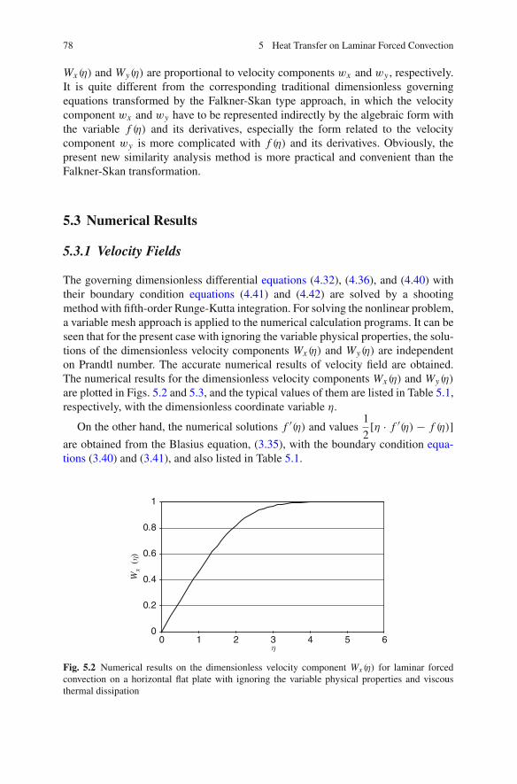
78 5 Heat Transfer on Laminar Forced Convection
Wx (η) and Wy(η) are proportional to velocity components wx and wy , respectively.It is quite different from the corresponding traditional dimensionless governingequations transformed by the Falkner-Skan type approach, in which the velocitycomponent wx and wy have to be represented indirectly by the algebraic form withthe variable f (η) and its derivatives, especially the form related to the velocitycomponent wy is more complicated with f (η) and its derivatives. Obviously, thepresent new similarity analysis method is more practical and convenient than theFalkner-Skan transformation.
5.3 Numerical Results
5.3.1 Velocity Fields
The governing dimensionless differential equations (4.32), (4.36), and (4.40) withtheir boundary condition equations (4.41) and (4.42) are solved by a shootingmethod with fifth-order Runge-Kutta integration. For solving the nonlinear problem,a variable mesh approach is applied to the numerical calculation programs. It can beseen that for the present case with ignoring the variable physical properties, the solu-tions of the dimensionless velocity components Wx (η) and Wy(η) are independenton Prandtl number. The accurate numerical results of velocity field are obtained.The numerical results for the dimensionless velocity components Wx (η) and Wy(η)
are plotted in Figs. 5.2 and 5.3, and the typical values of them are listed in Table 5.1,respectively, with the dimensionless coordinate variable η.
On the other hand, the numerical solutions f ′(η) and values1
2[η · f ′(η)− f (η)]
are obtained from the Blasius equation, (3.35), with the boundary condition equa-tions (3.40) and (3.41), and also listed in Table 5.1.
0
0.2
0.4
0.6
0.8
1
0 1 2 3 4 5 6
Wx
(η)
η
Fig. 5.2 Numerical results on the dimensionless velocity component Wx (η) for laminar forcedconvection on a horizontal flat plate with ignoring the variable physical properties and viscousthermal dissipation
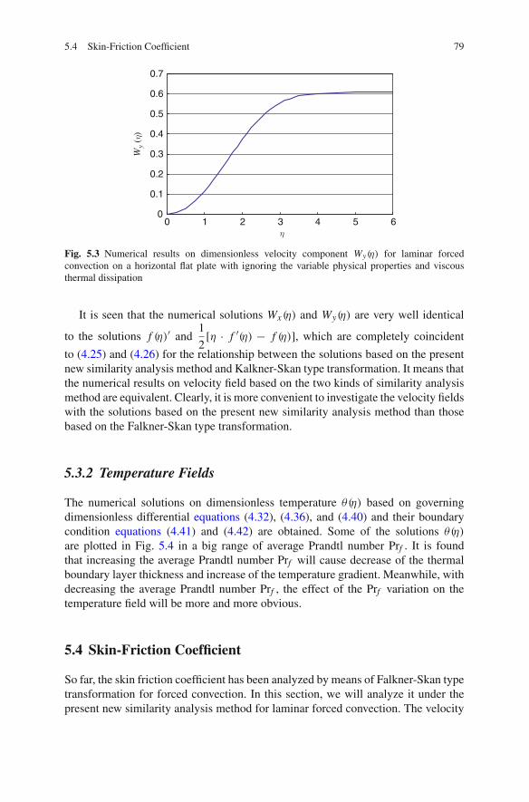
5.4 Skin-Friction Coefficient 79
0
0.1
0.2
0.3
0.4
0.5
0.6
0.7
0 1 2 3 4 5 6
Wy
(η)
η
Fig. 5.3 Numerical results on dimensionless velocity component Wy(η) for laminar forcedconvection on a horizontal flat plate with ignoring the variable physical properties and viscousthermal dissipation
It is seen that the numerical solutions Wx (η) and Wy(η) are very well identical
to the solutions f (η)′ and1
2[η · f ′(η) − f (η)], which are completely coincident
to (4.25) and (4.26) for the relationship between the solutions based on the presentnew similarity analysis method and Kalkner-Skan type transformation. It means thatthe numerical results on velocity field based on the two kinds of similarity analysismethod are equivalent. Clearly, it is more convenient to investigate the velocity fieldswith the solutions based on the present new similarity analysis method than thosebased on the Falkner-Skan type transformation.
5.3.2 Temperature Fields
The numerical solutions on dimensionless temperature θ(η) based on governingdimensionless differential equations (4.32), (4.36), and (4.40) and their boundarycondition equations (4.41) and (4.42) are obtained. Some of the solutions θ(η)are plotted in Fig. 5.4 in a big range of average Prandtl number Prf . It is foundthat increasing the average Prandtl number Prf will cause decrease of the thermalboundary layer thickness and increase of the temperature gradient. Meanwhile, withdecreasing the average Prandtl number Prf , the effect of the Prf variation on thetemperature field will be more and more obvious.
5.4 Skin-Friction Coefficient
So far, the skin friction coefficient has been analyzed by means of Falkner-Skan typetransformation for forced convection. In this section, we will analyze it under thepresent new similarity analysis method for laminar forced convection. The velocity

80 5 Heat Transfer on Laminar Forced Convection
Table 5.1 Numerical solutions related to velocity field respectively based on the Falkner-Skantype transformation and the present new similarity analysis method for laminar forced convectionon a horizontal flat plate without consideration of variable thermophysical properties and viscousthermal dissipation
η
Solutions of (3.35) (transformed byFalkner-Skan pe transformation)
Solutions of (4.32) and (4.36)(transformed by the newsimilarity analysis method)
f (η) f ′(η) 1
2[η · f ′(η)− f (η)] Wy(η) Wx (η)
0 0 0 0 0 00.2 0.009391 0.093905 0.004695 0.004695 0.0939050.4 0.037549 0.187505 0.018727 0.018746 0.1876050.6 0.084386 0.280505 0.041959 0.04198 0.2805760.8 0.149575 0.371963 0.073998 0.073948 0.3719641 0.232990 0.460632 0.113821 0.113821 0.4606331.2 0.333657 0.545246 0.160319 0.160319 0.5452471.4 0.450723 0.624386 0.211709 0.211709 0.6243871.6 0.582956 0.696699 0.265881 0.265882 0.69671.8 0.728872 0.761057 0.320515 0.320516 0.7610582 0.886796 0.816694 0.373296 0.373297 0.8166952.2 1.054946 0.863303 0.42216 0.422161 0.8633052.4 1.231527 0.901065 0.465515 0.465515 0.9010662.6 1.414823 0.930601 0.50237 0.50237 0.9306022.8 1.603282 0.952875 0.532384 0.532384 0.9528763 1.795567 0.969054 0.555798 0.555798 0.9690553.2 1.990580 0.980365 0.573294 0.573294 0.9803663.4 2.187466 0.987970 0.585816 0.585816 0.9879713.6 2.385589 0.992888 0.594404 0.594403 0.9928893.8 2.584497 0.995944 0.600045 0.600045 0.9959454 2.783885 0.997770 0.603598 0.603597 0.9977714.2 2.983554 0.998818 0.605741 0.605741 0.9988194.4 3.183381 0.999396 0.606981 0.606981 0.9993974.6 3.383294 0.999703 0.60767 0.607669 0.9997044.8 3.583252 0.999859 0.608036 0.608036 0.999865 3.783232 0.999936 0.608224 0.608222 0.9999375.2 3.983224 0.999971 0.608313 0.608314 0.9999735.4 4.183220 0.999988 0.608358 0.608357 0.9999895.6 4.383218 0.999995 0.608377 0.608376 0.9999965.8 4.583217 0.999998 0.608386 0.608385 0.9999996 4.783217 0.999999 0.608389 0.608388 1
gradient at the wall is important characteristic of the solution, and the local skin-friction coefficient C f,x is a dimensionless measure of the shear stress at the wall, i.e.
Cx, f = τw,x
1
2ρfw2
x,∞=μ f
(∂wx
∂y
)
y=0
1
2ρfw2
x,∞. (5.1)
With (4.23), we have
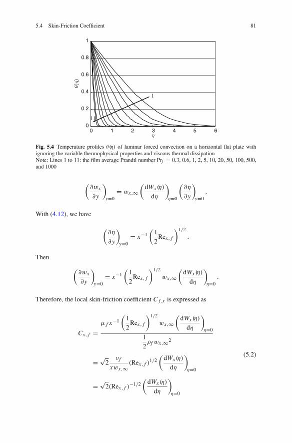
5.4 Skin-Friction Coefficient 81
0
0.2
0.4
0.6
0.8
1
0 1 2 3 4 5 6
1
11
θ(η)
η
Fig. 5.4 Temperature profiles θ(η) of laminar forced convection on a horizontal flat plate withignoring the variable thermophysical properties and viscous thermal dissipationNote: Lines 1 to 11: the film average Prandtl number Prf = 0.3, 0.6, 1, 2, 5, 10, 20, 50, 100, 500,and 1000
(∂wx
∂y
)
y=0= wx,∞
(dWx (η)
dη
)
η=0
(∂η
∂y
)
y=0.
With (4.12), we have
(∂η
∂y
)
y=0= x−1
(1
2Rex, f
)1/2
.
Then
(∂wx
∂y
)
y=0= x−1
(1
2Rex, f
)1/2
wx,∞(
dWx (η)
dη
)
η=0.
Therefore, the local skin-friction coefficient C f,x is expressed as
Cx, f =μ f x−1
(1
2Rex, f
)1/2
wx,∞(
dWx (η)
dη
)
η=0
1
2ρfwx,∞2
= √2
νf
xwx,∞(Rex, f )
1/2(
dWx (η)
dη
)
η=0
= √2(Rex, f )
−1/2(
dWx (η)
dη
)
η=0
(5.2)

82 5 Heat Transfer on Laminar Forced Convection
Since the numerical solution
(dWx (η)
dη
)
η=0= 0.4696, the well-known expression
of local skin friction coefficient Cx, f is obtained as
Cx, f == 0.664(Rex, f )−1/2 (5.3)
for laminar forced convection on a horizontal flat plate.The average skin friction coefficient from x = 0 to x is described as
Cx, f = 1
x
∫ x
0Cx, f dx = 0.664
1
x
∫ x
0(Rex, f )
−1/2dx = 1.328Re−1/2x, f . (5.4)
5.5 Heat Transfer
5.5.1 Heat Transfer Analysis
The local heat transfer rate (qx, f )Ec=0 at position x per unit area from the surface ofthe plate with ignoring the viscous thermal dissipation and variable physical prop-erties can be calculated by Fourier’s law as
(qx, f )Ec=0 = −λf
[(∂t
∂y
)
y=0
]
f,Ec=0
.
The subscript Ec = 0 demonstrates that in the related investigation the viscousthermal dissipation is not considered, and the subscript f denotes the case that
the boundary layer average temperature tf = tw + t∞2
is taken as the reference
temperature with ignoring the variable physical properties.With (4.7), (4.12), and (4.27), we have
(qx, f )Ec=0 = −λf (tw − t∞)[(
dθ(η)
dη
)
η=0
]
f,Ec=0
∂η
∂y,
(qx, f )Ec=0 = λf (tw − t∞)(
1
2Rex, f
)1/4
x−1
[−(
dθ(η)
dη
)
η=0
]
f,Ec=0
. (5.5)
It should be indicated that in analysis and calculation of this chapter, the viscousthermal dissipation is not considered in the energy governing differential equation,and then the corresponding wall temperature gradient and local heat transfer rate
are expressed as
[−(
dθ(η)
dη
)
η=0
]
f,Ec=0
and (qx, f )Ec=0. In next chapter, we will
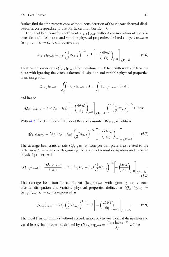
5.5 Heat Transfer 83
further find that the present case without consideration of the viscous thermal dissi-pation is corresponding to that for Eckert number Ec = 0.
The local heat transfer coefficient [αx, f ]Ec=0 without consideration of the vis-cous thermal dissipation and variable physical properties, defined as (qx, f )Ec=0 =(αx, f )Ec=0(tw − t∞), will be given by
(αx, f )Ec=0 = λ f
(1
2Rex, f
)1/2
x−1
[−(
dθ(η)
dη
)
η=0
]
f,Ec=0
. (5.6)
Total heat transfer rate (Qx, f )Ec=0 from position x = 0 to x with width of b on theplate with ignoring the viscous thermal dissipation and variable physical propertiesis an integration
(Qx, f)Ec=0 =∫∫
A
[qx, f ]Ec=0 dA =∫ x
0[qx, f ]Ec=0 b · dx,
and hence
(Qx, f )Ec=0 = λf b(tw − t∞)[−(
dθ(η)
dη
)
η=0
]
f,Ec=0
∫ x
0
(1
2Rex, f
)1/2
x−1dx .
With (4.7) for definition of the local Reynolds number Rex, f , we obtain
(Qx, f)Ec=0 = 2bλf (tw − t∞)(
1
2Rex, f
)1/2[−(
dθ(η)
dη
)
η=0
]
f,Ec=0
. (5.7)
The average heat transfer rate (Qx, f )Ec=0 from per unit plate area related to theplate area A = b × x with ignoring the viscous thermal dissipation and variablephysical properties is
(Qx, f)Ec=0 = (Qx, f)Ec=0
b × x= 2x−1λf (tw − t∞)
(1
2Rex, f
)1/2[−(dθ(η)
dη
)
η=0
]
f,Ec=0
.
(5.8)
The average heat transfer coefficient ([αx, f )Ec=0 with ignoring the viscousthermal dissipation and variable physical properties defined as (Qx, f )Ec=0 =(αx, f )Ec=0(tw − t∞) is expressed as
(αx, f )Ec=0 = 2λf
(1
2Rex, f
)1/2
x−1
[−(
dθ(η)
dη
)
η=0
]
f,Ec=0
. (5.9)
The local Nusselt number without consideration of viscous thermal dissipation and
variable physical properties defined by (Nux, f )Ec=0 = [αx, f ]Ec=0 · x
λfwill be

84 5 Heat Transfer on Laminar Forced Convection
(Nux, f )Ec=0 = λf
(1
2Rex, f
)1/2
x−1
[−(
dθ(η)
dη
)
η=0
]
f,Ec=0
x
λf,
i.e.
(Nux, f )Ec=0 =(
1
2Rex, f
)1/2[−(
dθ(η)
dη
)
η=0
]
f,Ec=0
. (5.10)
The average Nusselt number without consideration of variable thermal dissipation
and variable thermophysical properties is defined as (Nux, f )Ec=0 = (αx, f )Ec=0 x
λf,
and hence
(Nux, f )Ec=0 = 2
(1
2Rex, f
)1/2[−(
dθ(η)
dη
)
η=0
]
f,Ec=0
,
i.e.
(Nux, f )Ec=0 = √2Rex, f
1/2
[−(
dθ(η)
dη
)
η=0
]
f,Ec=0
. (5.11)
5.5.2 Dimensionless Wall Temperature Gradient
In the heat transfer equations (5.5) to (5.11) obtained by heat transfer analysis, the
dimensionless temperature gradient
[−(
dθ(η)
dη
)
η=0
]
f,Ec=0
is only one no-given
variable for prediction of heat transfer. Then, evaluation of the dimensionless tem-
perature gradient
[−(
dθ(η)
dη
)
η=0
]
f,Ec=0
becomes the important issue for the pre-
diction of heat transfer results.From Fig. 5.4, it is clear that the wall dimensionless temperature gradient[
−(
dθ(η)
dη
)
η=0
]
f,Ec=0
varies with Prandtl number Pr f . A system of the numerical
results of the wall temperature gradients
[−(
dθ(η)
dη
)
η=0
]
f,Ec=0
is obtained and
plotted in Fig. 5.5, and some typical values are listed in Table 5.2. It is clear thatdecrease of average Prandtl number Prf will cause decrease of the wall temperature
gradient
[−(
dθ(η)
dη
)
η=0
]
f,Ec=0
at an accelerative pace.

5.5 Heat Transfer 85
0
0.5
1
1.5
2
2.5
0 20 40 60 80 100Prf
[−(
)η
= 0]
f, E
c = 0
dθ (η
)dη
Fig. 5.5 Numerical solutions on wall temperature gradient
[−(
dθ(η)
dη
)
η=0
]
f,Ec=0
of laminar
forced convection on a horizontal plate with ignoring the viscous thermal dissipation
Table 5.2 Numerical solutions and the predicted values for the wall temperature gradients[−(
dθ(η)
dη
)
η=0
]
f,Ec=0
as well as their predicted deviations by using (5.12) for laminar forced con-
vection on a horizontal flat plate with ignoring the viscous thermal dissipation and variable physicalproperties
[−(
dθ(η)
dη
)
η=0
]
f,Ec=0
Numerical Predicted by Deviation predictedPrf Solution (5.12) by (5.12)
0.3 0.30401 0.314366 3.34%0.6 0.391718 0.396076 1.11%1 0.469601 0.4696 02 0.597234 0.591659 −0.93%3 0.686202 0.67728 −1.3%5 0.815561 0.803005 −1.54%10 1.029735 1.011723 −1.75%20 1.298819 1.274691 −1.86%30 1.487318 1.459156 −1.89%50 1.763922 1.730021 −1.92%70 1.97446 1.935356 −1.98%100 2.222905 2.17969 −1.94%
By using a curve-matching approach, the numerical results of[−(
dθ(η)
dη
)
η=0
]
f,Ec=0
for
ignoring the thermal viscous dissipation and variable physical properties are here
formulated to (5.12). Meanwhile, the values of[−(
dθ(η)
dη
)
η=0
]
f,Ec=0
predicted by (5.12)
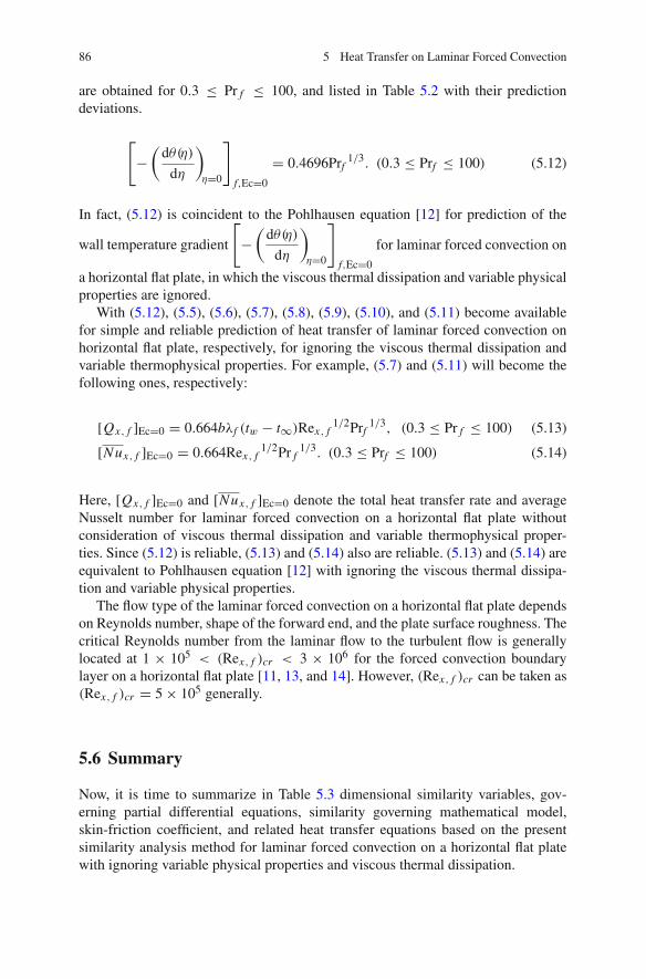
86 5 Heat Transfer on Laminar Forced Convection
are obtained for 0.3 ≤ Pr f ≤ 100, and listed in Table 5.2 with their predictiondeviations.
[−(
dθ(η)
dη
)
η=0
]
f,Ec=0
= 0.4696Prf1/3. (0.3 ≤ Prf ≤ 100) (5.12)
In fact, (5.12) is coincident to the Pohlhausen equation [12] for prediction of the
wall temperature gradient
[−(
dθ(η)
dη
)
η=0
]
f,Ec=0
for laminar forced convection on
a horizontal flat plate, in which the viscous thermal dissipation and variable physicalproperties are ignored.
With (5.12), (5.5), (5.6), (5.7), (5.8), (5.9), (5.10), and (5.11) become availablefor simple and reliable prediction of heat transfer of laminar forced convection onhorizontal flat plate, respectively, for ignoring the viscous thermal dissipation andvariable thermophysical properties. For example, (5.7) and (5.11) will become thefollowing ones, respectively:
[Qx, f ]Ec=0 = 0.664bλf (tw − t∞)Rex, f1/2Prf
1/3, (0.3 ≤ Pr f ≤ 100) (5.13)
[Nux, f ]Ec=0 = 0.664Rex, f1/2Pr f
1/3. (0.3 ≤ Prf ≤ 100) (5.14)
Here, [Qx, f ]Ec=0 and [Nux, f ]Ec=0 denote the total heat transfer rate and averageNusselt number for laminar forced convection on a horizontal flat plate withoutconsideration of viscous thermal dissipation and variable thermophysical proper-ties. Since (5.12) is reliable, (5.13) and (5.14) also are reliable. (5.13) and (5.14) areequivalent to Pohlhausen equation [12] with ignoring the viscous thermal dissipa-tion and variable physical properties.
The flow type of the laminar forced convection on a horizontal flat plate dependson Reynolds number, shape of the forward end, and the plate surface roughness. Thecritical Reynolds number from the laminar flow to the turbulent flow is generallylocated at 1 × 10⁵ < (Rex, f )cr < 3 × 10⁶ for the forced convection boundarylayer on a horizontal flat plate [11, 13, and 14]. However, (Rex, f )cr can be taken as(Rex, f )cr = 5 × 10⁵ generally.
5.6 Summary
Now, it is time to summarize in Table 5.3 dimensional similarity variables, gov-erning partial differential equations, similarity governing mathematical model,skin-friction coefficient, and related heat transfer equations based on the presentsimilarity analysis method for laminar forced convection on a horizontal flat platewith ignoring variable physical properties and viscous thermal dissipation.
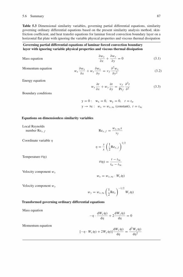
5.6 Summary 87
Table 5.3 Dimensional similarity variables, governing partial differential equations, similaritygoverning ordinary differential equations based on the present similarity analysis method, skin-friction coefficient, and heat transfer equations for laminar forced convection boundary layer on ahorizontal flat plate with ignoring the variable physical properties and viscous thermal dissipation
Governing partial differential equations of laminar forced convection boundarylayer with ignoring variable physical properties and viscous thermal dissipation
Mass equation∂wx
∂x+ ∂wy
∂y= 0 (3.1)
Momentum equationwx∂wx
∂x+ wy
∂wx
∂y= ν f
∂2wx
∂y2(3.2)
Energy equation
wx∂t
∂x+ wy
∂t
∂y= ν f
Pr f
∂2t
∂2(3.3)
Boundary conditions
y = 0 : wx = 0, wy = 0, t = twy → ∞ : wx = wx,∞ (constant), t = t∞
Equations on dimensionless similarity variables
Local Reynoldsnumber Rex, f Rex, f = wx,∞x
νf
Coordinate variable η
η = y
x
(1
2Rex, f
)1/2
Temperature θ(η)
θ(η) = t − t∞tw − t∞
Velocity component wxwx = wx,∞ · Wx (η)
Velocity component wy
wy = wx,∞(
1
2Rex
)−1/2
Wy(η)
Transformed governing ordinary differential equations
Mass equation
−η · dWx (η)
dη+ 2
dWy(η)
dη= 0
Momentum equation
[−η · Wx (η)+ 2Wy(η)]dWx (η)
dη= d2Wx (η)
dη2

88 5 Heat Transfer on Laminar Forced Convection
Table 5.3 (continued)
Energy equation
[−η · Wx (η)+ 2Wy(η)]dθ(η)
dη= 1
Pr f
d2θ(η)
dη2
Boundary conditions
η = 0 : Wx (η) = 0,Wy(η) = 0, θ(η) = 1
η → ∞ : Wx (η) = 1, θ(η) = 0
Skin-friction coefficient
Local skin-frictioncoefficient C f,x Cx, f == 0.664Rex, f
−1/2
Average skin-frictioncoefficient Cx, f C x, f = 1.328Rex, f
−1/2
Equations related to heat transfer
[−(
dθ(η)
dη
)
η=0
]
f,Ec=0
[−(
dθ(η)
dη
)
η=0
]
f,Ec=0
= 0.4696Prf1/3 (0.3 ≤ Prf ≤ 100)
Local values(Nux, f )Ec=0 =[αx, f ]Ec=0 · x
λf
(qx, f )Ec=0 = λf (tw − t∞)(
1
2Rex, f
)1/4
x−1
[−(
dθ(η)
dη
)
η=0
]
f,Ec=0
(Nux, f )Ec=0 =(
1
2Rex, f
)1/2[−(
dθ(η)
dη
)
η=0
]
f,Ec=0
Average values(Nux, f )Ec=0 =(αx, f )Ec=0x
λf
(Qx, f )Ec=0 = 2x−1λf (tw − t∞)(
1
2Rex, f
)1/2[−(
dθ(η)
dη
)
η=0
]
f,Ec=0
(Nux, f )Ec=0 = √2Rex, f
1/2
[−(
dθ(η)
dη
)
η=0
]
f,Ec=0
Total value
(Qx, f )Ec=0 = 2bλf (tw − t∞)(
1
2Rex, f
)1/2[−(
dθ(η)
dη
)
η=0
]
f,Ec=0
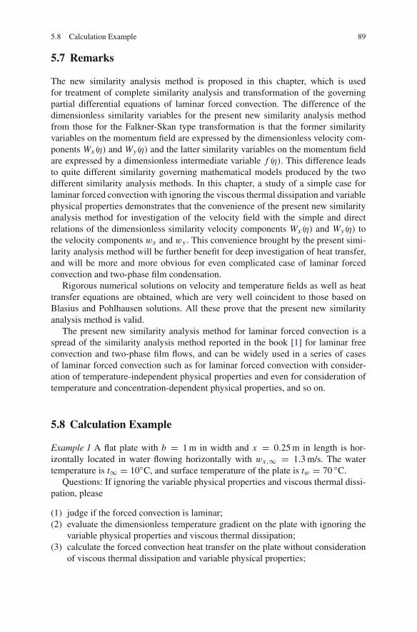
5.8 Calculation Example 89
5.7 Remarks
The new similarity analysis method is proposed in this chapter, which is usedfor treatment of complete similarity analysis and transformation of the governingpartial differential equations of laminar forced convection. The difference of thedimensionless similarity variables for the present new similarity analysis methodfrom those for the Falkner-Skan type transformation is that the former similarityvariables on the momentum field are expressed by the dimensionless velocity com-ponents Wx (η) and Wy(η) and the latter similarity variables on the momentum fieldare expressed by a dimensionless intermediate variable f (η). This difference leadsto quite different similarity governing mathematical models produced by the twodifferent similarity analysis methods. In this chapter, a study of a simple case forlaminar forced convection with ignoring the viscous thermal dissipation and variablephysical properties demonstrates that the convenience of the present new similarityanalysis method for investigation of the velocity field with the simple and directrelations of the dimensionless similarity velocity components Wx (η) and Wy(η) tothe velocity components wx and wy . This convenience brought by the present simi-larity analysis method will be further benefit for deep investigation of heat transfer,and will be more and more obvious for even complicated case of laminar forcedconvection and two-phase film condensation.
Rigorous numerical solutions on velocity and temperature fields as well as heattransfer equations are obtained, which are very well coincident to those based onBlasius and Pohlhausen solutions. All these prove that the present new similarityanalysis method is valid.
The present new similarity analysis method for laminar forced convection is aspread of the similarity analysis method reported in the book [1] for laminar freeconvection and two-phase film flows, and can be widely used in a series of casesof laminar forced convection such as for laminar forced convection with consider-ation of temperature-independent physical properties and even for consideration oftemperature and concentration-dependent physical properties, and so on.
5.8 Calculation Example
Example 1 A flat plate with b = 1 m in width and x = 0.25 m in length is hor-izontally located in water flowing horizontally with wx,∞ = 1.3 m/s. The watertemperature is t∞ = 10◦C, and surface temperature of the plate is tw = 70 ◦C.
Questions: If ignoring the variable physical properties and viscous thermal dissi-pation, please
(1) judge if the forced convection is laminar;(2) evaluate the dimensionless temperature gradient on the plate with ignoring the
variable physical properties and viscous thermal dissipation;(3) calculate the forced convection heat transfer on the plate without consideration
of viscous thermal dissipation and variable physical properties;
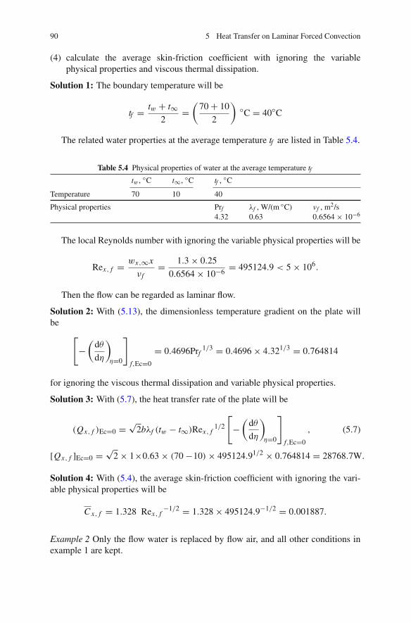
90 5 Heat Transfer on Laminar Forced Convection
(4) calculate the average skin-friction coefficient with ignoring the variablephysical properties and viscous thermal dissipation.
Solution 1: The boundary temperature will be
tf = tw + t∞2
=(
70 + 10
2
)◦C = 40◦C
The related water properties at the average temperature tf are listed in Table 5.4.
Table 5.4 Physical properties of water at the average temperature tf
tw , ◦C t∞, ◦C tf , ◦C
Temperature 70 10 40
Physical properties Prf λf , W/(m ◦C) νf , m2/s4.32 0.63 0.6564 × 10⁻⁶
The local Reynolds number with ignoring the variable physical properties will be
Rex, f = wx,∞x
νf= 1.3 × 0.25
0.6564 × 10−6= 495124.9 < 5 × 10⁶.
Then the flow can be regarded as laminar flow.
Solution 2: With (5.13), the dimensionless temperature gradient on the plate willbe
[−(
dθ
dη
)
η=0
]
f,Ec=0
= 0.4696Prf1/3 = 0.4696 × 4.321/3 = 0.764814
for ignoring the viscous thermal dissipation and variable physical properties.
Solution 3: With (5.7), the heat transfer rate of the plate will be
(Qx, f )Ec=0 = √2bλf (tw − t∞)Rex, f
1/2
[−(
dθ
dη
)
η=0
]
f,Ec=0
, (5.7)
[Qx, f ]Ec=0 = √2 × 1×0.63 × (70 −10)× 495124.91/2 × 0.764814 = 28768.7W.
Solution 4: With (5.4), the average skin-friction coefficient with ignoring the vari-able physical properties will be
Cx, f = 1.328 Rex, f−1/2 = 1.328 × 495124.9−1/2 = 0.001887.
Example 2 Only the flow water is replaced by flow air, and all other conditions inexample 1 are kept.

5.8 Calculation Example 91
Questions:
(1) Please judge if the forced convection is laminar;(2) Please evaluate the dimensionless temperature gradient on the plate with ignor-
ing the variable physical properties and viscous thermal dissipation;(3) Please calculate the forced convection heat transfer on the plate without
consideration of viscous thermal dissipation and variable physical properties;(4) Please calculate the average skin-friction coefficient with ignoring the variable
physical properties and viscous thermal dissipation.
Solution 1: The related air properties at the average temperature tf are listed inTable 6.5.
Table 5.5 Physical properties of air at the average temperature tf
tw , ◦C t∞, ◦C tf , ◦C
Temperature 70 10 40
Physical properties Prf λf , W/(m ◦C) ν f , m2/s
0.7 0.02726 17.20 × 10⁻⁶
The local Reynolds number will be
Rex, f = wx,∞x
νf= 1.3 × 0.25
17.20 × 10−6= 18895.3 < 5 × 10⁵.
Then the flow can be regarded as laminar flow.
Solution 2: With (5.13), the dimensionless temperature gradient on the plate willbe
[−(
dθ
dη
)
η=0
]
f,Ec=0
= 0.4696Prf1/3 = 0.4696 × 0.71/3 = 0.41696
for ignoring the viscous thermal dissipation and variable physical properties.
Solution 3: With (5.7), the forced convection heat transfer result of air laminarforced convection with ignoring viscous thermal dissipation and variable physicalproperties will be
[Qx, f ]Ec=0 = √2bλf (tw − t∞)Rex, f
1/2
[−(
dθ
dη
)
η=0
]
f,Ec=0
,
= √2 × 1 × 0.02726 × (70 − 10)× 18895.31/2 × 0.41696,
= 132.6 W.

92 5 Heat Transfer on Laminar Forced Convection
Solution 4: With (5.4), the average skin-friction coefficient with ignoring variablephysical properties is calculated as
Cx, f = 1.328 Rex, f−1/2 = 1.328 × 18895.3−1/2 = 0.009661.
Exercise
1. Follow example 1. Only the wall temperature is changed to 90◦C, and all otherconditions are kept.Questions: If ignoring the variable physical properties and viscous thermal dis-sipation, please
(1) judge if the forced convection is laminar;(2) evaluate the dimensionless temperature gradient on the plate by ignoring the
variable physical properties and viscous thermal dissipation;(3) calculate the forced convection heat transfer on the plate by ignoring the
variable physical properties and viscous thermal dissipation;(4) calculate the average skin-friction coefficient by ignoring the variable phys-
ical properties and viscous thermal dissipation.
References
1. H. Blasius, Grenzschichten in Flussigkeiten mit kleiner Reibung, Z. Math. Phys. 56, 1–37(1908)
2. V.M. Falkner, S.W. Skan, Some approximate solutions of the boundary layer Equations. Phil.Mag, 12, 865 (1931)
3. E.R.G. Eckert, R.M. Drake, Analysis of heat and mass transfer. (McGraw-Hill, NewYork, NY,1972)
4. T. Cebeci, P. Bradshaw, Physical and Computational aspects of convective heat transfer.(Springer, New York, NY, 1984)
5. T. Fujii, Theory of Laminar Film Condensation. (Springer, New York, NY, 1991)6. B. Louis, etc., Convective Heat Transfer, 2nd edn, (John Wiley & sons, Inc., 1993)7. S. Kakaç, Y. Yenner Convective Heat Transfer, 2nd edn, CRC Press, 1995)8. A. Bejan, Convection Heat Transfer, 2nd edn, (Wiley, New York, NY, 1995)9. I. Pop, D.B. Ingham, Convective heat transfer – Mathematical and Computational Modelling
of Viscous Fluids and Porous Media (Elsevier, Amsterdam, 2001)10. T. Cebeci, Convective Heat Transfer, 2nd edn, (Springer, Heidelberg, 2002)11. H. Schlichting, Boundary-Layer Theory (Springer, Heidelberg, 2004)12. E. Pohlhausen, Der Wärmeaustausch zwischen festen Körpern und Flüssigkeiten mit kleiner
Reibung und kleiner Wärmeleitung. Z. Angew. Math. Mech. 1, 115–121, (1921)13. J.H. Lienhard, A Heat Transfer Textbook, (Prentice-Hall, Englewood Cliffs, 1981)14. S.W. Churchill, A comprehensive correlating equation for forced convection from flat plates.
AICHE J. 22(2), 264–268, (1976)

Chapter 6Heat Transfer of Laminar Forced Convectionwith Consideration of Viscous ThermalDissipation
Abstract The present new similarity analysis method is used for extensive studyon heat transfer of laminar forced convection with consideration of viscous thermaldissipation. The proposed expressions of the dimensionless similarity velocity com-ponents related to the momentum field are proportional to the related velocity com-ponents, and it is obvious that the similarity governing mathematical model based onthe present new similarity analysis method is more clear and direct than that trans-formed by the Falkner-Skan type transformation. With the complete similarity gov-erning mathematical model based on the new similarity analysis method, a systemof numerical solutions is found out in a wide range of the average Prandtl numberand Eckert number. With these numerical solutions, it is clear that: (i) Increasingthe Eckert number causes decrease of the positive heat transfer (from the wall toflow), and increase of the negative heat transfer (from the flow to the wall); and (ii)Increase of the Prandtl number will cause increase the effect of the viscous thermaldissipation on heat transfer. The system of key numerical solutions on wall dimen-sionless temperature gradient is formulated with the Eckert number and averagePrandtl number, and the formulated equations are so reliable that they are very wellcoincident to the related numerical results. Combined with the theoretical equa-tions on heat transfer, the formulated equations on wall dimensionless temperaturegradient can be used to predict heat transfer simply and reliably for considerationof viscous thermal dissipation and average Prandtl number. Additionally, deviationof heat transfer rate predicted by ignoring the viscous thermal dissipation is for-mulated for judgement of the validity for ignoring the viscous thermal dissipation.Furthermore, a system of the adiabatic Eckert numbers is formulated with variationof average Prandtl number for judgement of the heat flux direction. It is clear thatthe adiabatic Eckert number will increase at an accelerative pace with decrease ofthe average Prandtl number, especially in the region with lower Prandtl number.
6.1 Introduction
In treatment of energy equation of forced convection, the viscous thermal dissipationis usually neglected in a lot of previous theoretical analysis and calculation. Ignoringthe viscous thermal dissipation is equivalent to regard Eckert number Ec [1] as zero
D.Y. Shang, Theory of Heat Transfer with Forced Convection Film Flows,Heat and Mass Transfer, DOI 10.1007/978-3-642-12581-2_6,C© Springer-Verlag Berlin Heidelberg 2011
93

94 6 Heat Transfer of Laminar Forced Convection
in the dimensionless form of the energy equation. As we know, the Eckert number,
defined as Ec = w2
cp ·�t , expresses the ratio of a flow’s kinetic energy to the boundarylayer enthalpy difference, and is used to characterize viscous thermal dissipation ofconvection, especially for forced convection. So far, numerous investigations havebeen done for the effect of the viscous thermal dissipation on the fluid flows andheat transfer, such as those of [1–9], and some investigation results were furthercollected in a series books, such as [10, 11]. Those studies showed that in the fluidflows with high Eckert number, generated heat due to the viscous thermal dissipationdominates the fluid temperature, and then the Eckert number can never be taken aszero in the investigation of convection heat transfer.
Therefore, in theoretical study and engineering practice, it is very important toclarify the effect of viscous thermal dissipation on convection heat transfer, in orderto understand in which condition the Eckert number can be neglected without anyobvious deviation produced in the prediction result on heat transfer. In this presentwork, laminar forced convection on a horizontal flat plate is taken as an example forextensive investigation of these issues.
6.2 Governing Partial Differential Equations of LaminarForced Convection
6.2.1 Governing Partial Differential Equations
The physical model and co-ordinate system of boundary layer with two-dimensionallaminar forced convection are shown schematically in Fig. 5.1. A flat plate is hori-zontally located in parallel fluid flow with its mainstream velocity wx,∞. The platesurface temperature is tw and the fluid bulk temperature is t∞. Then, a velocityboundary layer is produced near the plate. If tw is not equal to t∞, a temperatureboundary layer will occur near the plate. We assume that the velocity boundarylayer is laminar. Then the governing partial differential equations (2.53), (2.56),and (2.58) for laminar forced convection boundary layer are simplified as followsfor consideration of the viscous thermal dissipation but with ignoring the variablephysical properties:
∂wx
∂x+ ∂wy
∂y= 0, (6.1)
wx∂wx
∂x+ wy
∂wx
∂y= νf
∂2wx
∂y2 , (6.2)
wx∂t
∂x+ wy
∂t
∂y= νf
Prf
∂2t
∂y2+ νf
cpf
(∂wx
∂y
)2
, (6.3)
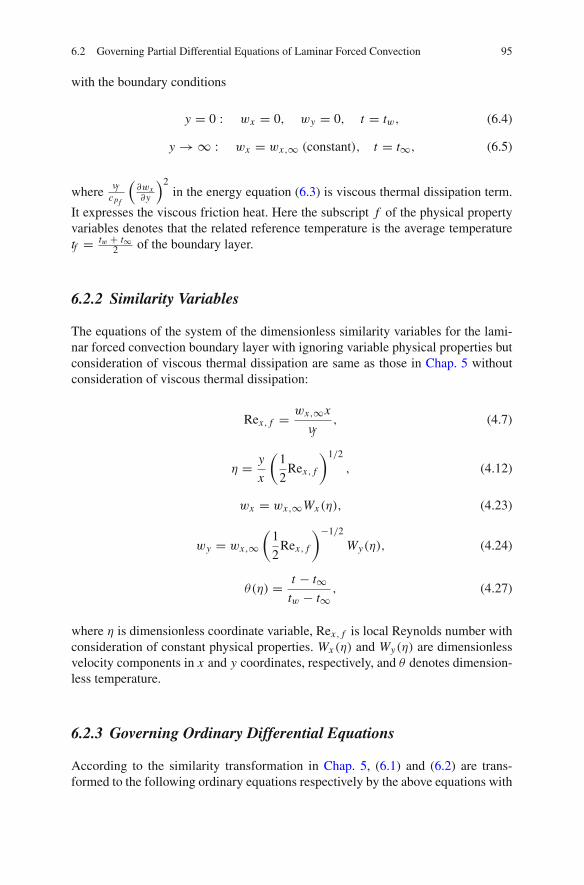
6.2 Governing Partial Differential Equations of Laminar Forced Convection 95
with the boundary conditions
y = 0 : wx = 0, wy = 0, t = tw, (6.4)
y → ∞ : wx = wx,∞ (constant), t = t∞, (6.5)
whereνf
cpf
(∂wx∂y
)2in the energy equation (6.3) is viscous thermal dissipation term.
It expresses the viscous friction heat. Here the subscript f of the physical propertyvariables denotes that the related reference temperature is the average temperaturetf = tw + t∞
2 of the boundary layer.
6.2.2 Similarity Variables
The equations of the system of the dimensionless similarity variables for the lami-nar forced convection boundary layer with ignoring variable physical properties butconsideration of viscous thermal dissipation are same as those in Chap. 5 withoutconsideration of viscous thermal dissipation:
Rex, f = wx,∞x
νf, (4.7)
η = y
x
(1
2Rex, f
)1/2
, (4.12)
wx = wx,∞Wx (η), (4.23)
wy = wx,∞(
1
2Rex, f
)−1/2
Wy(η), (4.24)
θ(η) = t − t∞tw − t∞
, (4.27)
where η is dimensionless coordinate variable, Rex, f is local Reynolds number withconsideration of constant physical properties. Wx (η) and Wy(η) are dimensionlessvelocity components in x and y coordinates, respectively, and θ denotes dimension-less temperature.
6.2.3 Governing Ordinary Differential Equations
According to the similarity transformation in Chap. 5, (6.1) and (6.2) are trans-formed to the following ordinary equations respectively by the above equations with
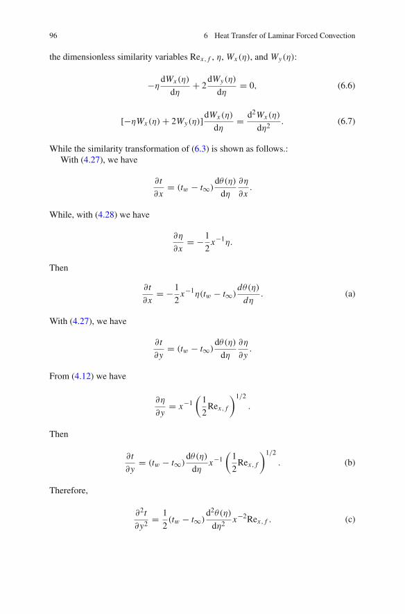
96 6 Heat Transfer of Laminar Forced Convection
the dimensionless similarity variables Rex, f , η, Wx (η), and Wy(η):
−ηdWx (η)
dη+ 2
dWy(η)
dη= 0, (6.6)
[−ηWx (η)+ 2Wy(η)]dWx (η)
dη= d2Wx (η)
dη2. (6.7)
While the similarity transformation of (6.3) is shown as follows.:With (4.27), we have
∂t
∂x= (tw − t∞)
dθ(η)
dη
∂η
∂x.
While, with (4.28) we have
∂η
∂x= −1
2x−1η.
Then
∂t
∂x= −1
2x−1η(tw − t∞)
dθ(η)
dη. (a)
With (4.27), we have
∂t
∂y= (tw − t∞)
dθ(η)
dη
∂η
∂y.
From (4.12) we have
∂η
∂y= x−1
(1
2Rex, f
)1/2
.
Then
∂t
∂y= (tw − t∞)
dθ(η)
dηx−1(
1
2Rex, f
)1/2
. (b)
Therefore,
∂2t
∂y2= 1
2(tw − t∞)
d2θ(η)
dη2x−2Rex, f . (c)

6.2 Governing Partial Differential Equations of Laminar Forced Convection 97
With (4.23), (4.24), (a), (b) and (c) and (4.34), (6.3) is changed to
− 1
2x−1ηwx,∞Wx (η)(tw − t∞)
dθ(η)
dη
+ wx,∞(
1
2Rex, f
)−1/2
Wy(η)(tw − t∞)dθ(η)
dηx−1(
1
2Rex, f
)1/2
= 1
2
ν f
Prf(tw − t∞)
d2θ(η)
dη2 x−2 Rex, f + ν f
cpf
[x−1(
1
2Rex, f
)1/2
wx,∞dWx (η)
dη
]2
With the definition of Rex, f , the above equation is further simplified to
− 1
2x−1ηwx,∞Wx (η)(tw − t∞)
dθ(η)
dη+ wx,∞Wy(η)(tw − t∞)
dθ(η)
dηx−1
= 1
2
ν f
Prf(tw − t∞)
d2θ(η)
dη2 x−2wx,∞x
ν f+ ν f
cpf
x−2(
1
2
wx,∞x
νf
)wx,∞2
(dWx (η)
dη
)2
.
With the definition of Reynolds number, the above equation is divided by 12 x−1
(tw − t∞)wx,∞, and simplified to
[−η · Wx (η)+ 2 · Wy(η)]dθ(η)
dη= 1
Prf
d2θ(η)
dη2+ Ec
(dWx (η)
dη
)2
. (6.8)
The boundary condition equations (6.4) and (6.5) are transformed to the followingdimensionless ones:
η = 0 : Wx (η) = 0, Wy(η) = 0, θ(η) = 1, (6.9)
η → ∞ : Wx (η) = 1, θ(η) = 0, (6.10)
where
Ec = wx,∞2
cpf (tw − t∞)(6.11)
is the Eckert number for descript of the viscous thermal dissipation.
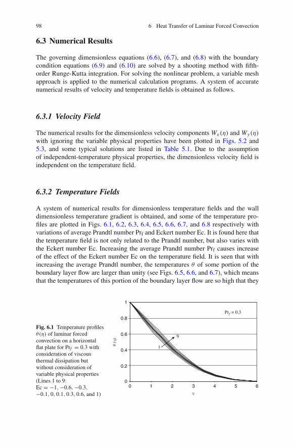
98 6 Heat Transfer of Laminar Forced Convection
6.3 Numerical Results
The governing dimensionless equations (6.6), (6.7), and (6.8) with the boundarycondition equations (6.9) and (6.10) are solved by a shooting method with fifth-order Runge-Kutta integration. For solving the nonlinear problem, a variable meshapproach is applied to the numerical calculation programs. A system of accuratenumerical results of velocity and temperature fields is obtained as follows.
6.3.1 Velocity Field
The numerical results for the dimensionless velocity components Wx (η) and Wy(η)
with ignoring the variable physical properties have been plotted in Figs. 5.2 and5.3, and some typical solutions are listed in Table 5.1. Due to the assumptionof independent-temperature physical properties, the dimensionless velocity field isindependent on the temperature field.
6.3.2 Temperature Fields
A system of numerical results for dimensionless temperature fields and the walldimensionless temperature gradient is obtained, and some of the temperature pro-files are plotted in Figs. 6.1, 6.2, 6.3, 6.4, 6.5, 6.6, 6.7, and 6.8 respectively withvariations of average Prandtl number Prf and Eckert number Ec. It is found here thatthe temperature field is not only related to the Prandtl number, but also varies withthe Eckert number Ec. Increasing the average Prandtl number Prf causes increaseof the effect of the Eckert number Ec on the temperature field. It is seen that withincreasing the average Prandtl number, the temperatures θ of some portion of theboundary layer flow are larger than unity (see Figs. 6.5, 6.6, and 6.7), which meansthat the temperatures of this portion of the boundary layer flow are so high that they
Fig. 6.1 Temperature profilesθ(η) of laminar forcedconvection on a horizontalflat plate for Prf = 0.3 withconsideration of viscousthermal dissipation butwithout consideration ofvariable physical properties(Lines 1 to 9:Ec = −1,−0.6,−0.3,−0.1, 0, 0.1, 0.3, 0.6, and 1)
0
0.2
0.4
0.6
0.8
1
0 1 2 3 4 5 6
9
Prf = 0.3
1θ (η
)
η

6.3 Numerical Results 99
Fig. 6.2 Temperature profilesθ(η) of laminar forcedconvection on a horizontalflat plate for Prf = 0.6 withconsideration of viscousthermal dissipation butwithout consideration ofvariable physical properties(Lines 1 to 9:Ec = −1,−0.6,−0.3,−0.1, 0, 0.1, 0.3, 0.6, and 1)
0
0.2
0.4
0.6
0.8
1
0 1 2 3 4 5 6
9
1
Prf = 0.6
θ (η
)
η
Fig. 6.3 Temperature profilesθ(η) of laminar forcedconvection on a horizontalflat plate for Prf = 1 withconsideration of viscousthermal dissipation butwithout consideration ofvariable physical properties(Lines 1 to 9:Ec = −1,−0.6,−0.3,−0.1, 0, 0.1, 0.3, 0.6, and 1)
00 1 2 3 4 5 6
0.2
0.4
0.6
0.8
1
1
9
θ (η
)
η
Prf = 1
Fig. 6.4 Temperature profilesθ(η) of laminar forcedconvection on a horizontalflat plate for Prf = 3 withconsideration of viscousthermal dissipation butwithout consideration ofvariable physical properties(lines 1 to 9:Ec = −1,−0.6,−0.3,−0.1, 0, 0.1, 0.3, 0.6, and 1)
0
0.2
0.4
0.6
0.8
1
1
9θ (η
)
0 1 2 3 4 5 6η
Prf = 3

100 6 Heat Transfer of Laminar Forced Convection
Fig. 6.5 Temperature profilesθ(η) of laminar forcedconvection on a horizontalflat plate for Prf = 10 withconsideration of viscousthermal dissipation butwithout consideration ofvariable physical properties(Lines 1 to 9:Ec = −1,−0.6,−0.3,−0.1, 0, 0.1, 0.3, 0.6, and 1)
0
0.2
0.4
0.6
0.8
1
1.2
0 1 2 3 4 5 6
θ (η
)
η
9
Prf = 10
1
Fig. 6.6 Temperature profilesθ(η) of laminar forcedconvection on a horizontalflat plate for Prf = 30 withconsideration of viscousthermal dissipation butwithout consideration ofvariable physical properties(Lines 1 to 9:Ec = −1,−0.6,−0.3,−0.1, 0, 0.1, 0.3, 0.6, and 1)
0
0.2
0.4
0.6
0.8
1
1.2
1.4
1
9
θ (η)
Prf = 30
0 1 2 3 4 5 6η
Fig. 6.7 Temperature profilesθ(η) of laminar forcedconvection on a horizontalflat plate for Prf = 100 withconsideration of viscousthermal dissipation butwithout consideration ofvariable physical properties(Lines 1 to 9:Ec = −1,−0.6,−0.3,−0.1, 0, 0.1, 0.3, 0.6, and 1)
0
0.2
0.4
0.6
0.8
1
1.2
1.4
1.6
1.8
2
1
9
0 1 2 3 4 5 6
θ (η
)
η
Prf = 100
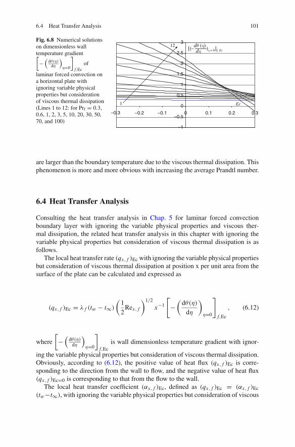
6.4 Heat Transfer Analysis 101
Fig. 6.8 Numerical solutionson dimensionless walltemperature gradient[−(
dθ(η)dη
)η=0
]
f,Ecof
laminar forced convection ona horizontal plate withignoring variable physicalproperties but considerationof viscous thermal dissipation(Lines 1 to 12: for Prf = 0.3,0.6, 1, 2, 3, 5, 10, 20, 30, 50,70, and 100)
[( )η = 0]f, Ec
–1
–0.5
0
1
1.5
2
2.5
3
–0.3 –0.2 –0.1 0 0.1 0.2 0.3
Ec1
12 dθ (η)dη−
0.5
are larger than the boundary temperature due to the viscous thermal dissipation. Thisphenomenon is more and more obvious with increasing the average Prandtl number.
6.4 Heat Transfer Analysis
Consulting the heat transfer analysis in Chap. 5 for laminar forced convectionboundary layer with ignoring the variable physical properties and viscous ther-mal dissipation, the related heat transfer analysis in this chapter with ignoring thevariable physical properties but consideration of viscous thermal dissipation is asfollows.
The local heat transfer rate (qx, f )Ec with ignoring the variable physical propertiesbut consideration of viscous thermal dissipation at position x per unit area from thesurface of the plate can be calculated and expressed as
(qx, f )Ec = λ f (tw − t∞)(
1
2Rex, f
)1/2
x−1
[−(
dθ(η)
dη
)
η=0
]
f,Ec
, (6.12)
where
[−(
dθ(η)dη
)η=0
]
f,Ecis wall dimensionless temperature gradient with ignor-
ing the variable physical properties but consideration of viscous thermal dissipation.Obviously, according to (6.12), the positive value of heat flux (qx, f )Ec is corre-sponding to the direction from the wall to flow, and the negative value of heat flux(qx, f )Ec=0 is corresponding to that from the flow to the wall.
The local heat transfer coefficient (αx, f )Ec, defined as (qx, f )Ec = (αx, f )Ec(tw−t∞), with ignoring the variable physical properties but consideration of viscous
102 6 Heat Transfer of Laminar Forced Convection
thermal dissipation will be given by
(αx, f )Ec = λ f
(1
2Rex, f
)1/2
x−1
[−(
dθ(η)
dη
)
η=0
]
f,Ec
. (6.13)
Total heat transfer rate (Qx, f )Ec from position x = 0 to x with width of b onthe plate with ignoring the variable physical properties but consideration of viscousthermal dissipation is
(Qx, f )Ec = √2bλ f (tw − t∞)Rex, f
1/2
[−(
dθ(η)
dη
)
η=0
]
f,Ec
. (6.14)
The average heat transfer rate (Qx,f)Ec from per unit plate area related to the platearea A = b × x with ignoring the variable physical properties but consideration ofviscous thermal dissipation is expressed as
(Qx, f )Ec = (Qx, f )Ec
b × x= √
2x−1λ f (tw − t∞)Rex, f1/2
[−(
dθ(η)
dη
)
η=0
]
f,Ec
. (6.15)
The average heat transfer coefficient (αx, f )Ec defined as (Qx, f )Ec(αx, f )Ec(tw−t∞)with ignoring the variable physical properties but consideration of viscous thermaldissipation is expressed as
(αx, f )Ec = √2λ f Rex, f
1/2x−1
[−(
dθ(η)
dη
)
η=0
]
f,Ec
. (6.16)
The local Nusselt number with ignoring variable physical properties but considera-tion of viscous thermal dissipation, defined by [Nux, f ]Ec = [αx, f ]Ec·x
λ f, will be
[Nux, f ]Ec =(
1
2Rex, f
)1/2[−(
dθ(η)
dη
)
η=0
]
f,Ec
. (6.17)
The average Nusselt number is defined as (Nux, f )Ec = (αx, f )Ec·xλ f
, with ignoringvariable physical properties but consideration of viscous thermal dissipation, andhence
(Nux, f )Ec = √2 Rex, f
1/2
[−(
dθ(η)
dη
)
η=0
]
f,Ec
. (6.18)
6.5 Formulated Equation of Dimensionless Wall Temperature Gradient 103
6.5 Formulated Equation of Dimensionless WallTemperature Gradient
It is found that in the heat transfer (6.12), (6.13), (6.14), (6.15), (6.16),(6.17), and (6.18) obtained by heat transfer analysis, the dimensionless tem-
perature gradient
[−(
dθ(η)dη
)η=0
]
f,Ecis only one no-given variable for the
prediction of heat transfer. In this section, we will further investigate itsevaluation so that the heat transfer results can be predicted simply andreliably.
Figures 6.1, 6.2, 6.3, 6.4, 6.5, 6.6, 6.7, and 6.8 demonstrate that the temperature
fields as well as the wall temperature gradient
[−(
dθ(η)dη
)η=0
]
f,Ecfor ignoring the
variable physical properties but consideration of viscous thermal dissipation varywith Prandtl number Pr f and Eckert number Ec. A system of the numerical results
of the wall temperature gradients
[−(
dθ(η)dη
)η=0
]
f,Ecare obtained and plotted in
Fig. 6.8, and some of them are listed in Table 6.1. It is clear that increasing the Eck-
ert number causes decrease of the wall temperature gradient
[−(
dθ(η)dη
)η=0
]
f,Ec.
On the other hand, increase of Prandtl number Prf will cause increase in the effectof the viscous thermal dissipation on the dimensionless wall temperature gradient[−(
dθ(η)dη
)η=0
]
f,Ec.
By using a curve-fitting approach, the dimensionless temperature gradient[−(
dθ(η)dη
)η=0
]
f,Ecwith ignoring variable physical properties but consideration
of viscous thermal dissipation is formulated based on the system of the rigorousnumerical solutions, i.e.
[−(
dθ(η)
dη
)
η=0
]
f,Ec
= a · Ec +[−(
dθ(η)
dη
)
η=0
]
f,Ec=0
,
(−0.1 ≤ Ec ≤ 0.1) and (0.3 ≤ Prf ≤ 3) (6.19)
[−(
dθ(η)
dη
)
η=0
]
f,Ec
= b · Ec2 + c · Ec +[−(
dθ(η)
dη
)
η=0
]
f,Ec=0
,
(−0.1 ≤ Ec ≤ 0.1) and (3 ≤ Prf ≤ 100) (6.20)

104 6 Heat Transfer of Laminar Forced Convection
Table 6.1 Numerical solutions and evaluated values on wall temperature gradient[−(
dθ(η)dη
)η=0
]
f,Ecof laminar forced convection on a horizontal plate with ignoring variable
physical properties but consideration of viscous thermal dissipation
Ec
−0.1 −0.03 −0.01 0 0.01 0.03 0.1
Prf
[−(
dθ(η)dη
)η=0
]
f,Ec
0.3 (1) 0.31224 0.306478 .304832 0.30401 0.303187 0.301542 0.29578(2) 0.322797 0.316895 0.315209 0.314366 0.31352 0.3118 0.30593(3) 0.0327 0.0329 0.0329 0.0329 0.0329 0.0330 0.0332
0.6 (1) 0.40685 0.396258 0.393231 0.39172 0.390204 0.387177 0.37658(2) 0.411049 0.400568 0.397573 0.396076 0.394579 0.391584 0.381103(3) 0.0102 0.01076 0.01092 0.011 0.0110 0.01125 0.0119
1 (1) 0.49308 0.476645 0.471949 0.46960 0.467252 0.462556 0.44612(2) 0.49291 0.476593 0.471931 0.4696 0.467269 0.462607 0.44629(3) −0.00034 −0.00011 −3.81E-05 0 3.64E-05 0.00011 0.00038
2 (1) 0.63925 0.609839 0.601436 0.59723 0.593033 0.584630 0.55522(2) 0.633879 0.604325 0.595880 0.591659 0.587437 0.578993 0.549439(3) −0.0085 −0.0091 −0.0093 −0.0094 −0.0095 −0.0097 −0.0105
3 (1) 0.74466 0.703738 0.692048 0.68620 0.680357 0.668666 0.62775(2) 0.736723 0.695115 0.683225 0.677280 0.671335 0.659445 0.61782384(3) −0.0108 −0.0124 −0.01291 −0.0132 −0.0134 −0.01398 −0.0161
5 (1) 0.90349 0.842056 0.824401 0.81556 0.806717 .789030 0.72712(2) 0.889663 0.829055 0.8116931 0.8030047 0.794311 0.776909 0.71584454(3) −0.0155 −0.0157 −0.0156 −0.0156 −0.0156 −0.0156 −0.0158
10 (1) 1.17655 1.074676 1.044835 1.02974 1.014506 .984024 0.87734(2) 1.159622 1.056645 1.026749 1.0117225 0.996643 0.966326 0.858559(3) −0.0146 −0.01706 −0.0176 −0.0178 −0.0179 −0.0183 −0.0218
20 (1) 1.53638 1.372632 1.323778 1.29882 1.272997 1.221358 1.04062(2) 1.513667 1.34856 1.299520 1.2746905 1.249653 1.198956 1.014989(3) −0.015 −0.01785 −0.0186 −0.0189 −0.0187 −0.01868 −0.0253
30 (1) 1.79972 1.584863 1.520512 1.48732 1.452399 1.382560 1.13813(2) 1.772507 1.55692 1.492103 1.4591563 1.425851 1.358166 1.109982(3) −0.0154 −0.0179 −0.01906 −0.01936 −0.0186 −0.0179 −0.0254
50 (1) 2.20267 1.901544 1.812972 1.76392 1.713498 1.612651 1.25969(2) 2.168313 1.86832 1.776772 1.730021 1.68262 1.585869 1.226785(3) −0.01584 −0.01778 −0.020374 −0.0195944 −0.01835 −0.01689 −0.026822
70 (1) 2.51602 2.145805 2.032571 1.97446 1.913859 1.783148 1.33413(2) 2.480924 2.108752 1.9940806 1.93535558 1.875704 1.753623 1.2971627(3) −0.01415 −0.01757 −0.0193 −0.0202 −0.02035 −0.01685 −0.0285
100 (1) 2.90624 2.441331 2.299284 2.22291 2.142979 1.979899 1.40442(2) 2.867333 2.399785 2.2543694 2.17969012 2.103696 1.947766 1.360603(3) −0.01357 −0.0173 −0.0199 −0.0198 −0.01867 −0.0165 −0.0322
Note: (1) numerical solution, (2) evaluated values by using (6.19) and (6.20), and (3) the evaluateddeviations
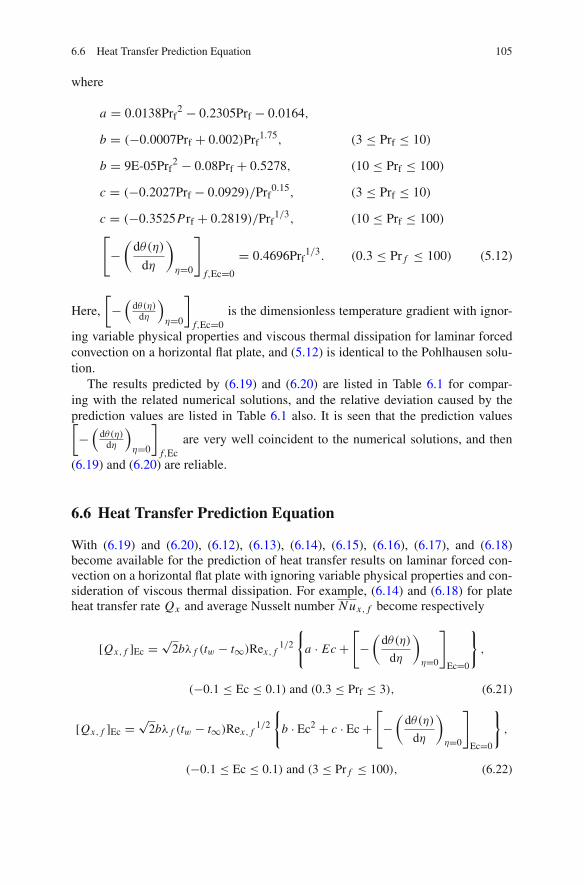
6.6 Heat Transfer Prediction Equation 105
where
a = 0.0138Prf2 − 0.2305Prf − 0.0164,
b = (−0.0007Prf + 0.002)Prf1.75, (3 ≤ Prf ≤ 10)
b = 9E-05Prf2 − 0.08Prf + 0.5278, (10 ≤ Prf ≤ 100)
c = (−0.2027Prf − 0.0929)/Prf0.15, (3 ≤ Prf ≤ 10)
c = (−0.3525Prf + 0.2819)/Prf1/3, (10 ≤ Prf ≤ 100)
[−(
dθ(η)
dη
)
η=0
]
f,Ec=0
= 0.4696Prf1/3. (0.3 ≤ Pr f ≤ 100) (5.12)
Here,
[−(
dθ(η)dη
)η=0
]
f,Ec=0is the dimensionless temperature gradient with ignor-
ing variable physical properties and viscous thermal dissipation for laminar forcedconvection on a horizontal flat plate, and (5.12) is identical to the Pohlhausen solu-tion.
The results predicted by (6.19) and (6.20) are listed in Table 6.1 for compar-ing with the related numerical solutions, and the relative deviation caused by theprediction values are listed in Table 6.1 also. It is seen that the prediction values[−(
dθ(η)dη
)η=0
]
f,Ecare very well coincident to the numerical solutions, and then
(6.19) and (6.20) are reliable.
6.6 Heat Transfer Prediction Equation
With (6.19) and (6.20), (6.12), (6.13), (6.14), (6.15), (6.16), (6.17), and (6.18)become available for the prediction of heat transfer results on laminar forced con-vection on a horizontal flat plate with ignoring variable physical properties and con-sideration of viscous thermal dissipation. For example, (6.14) and (6.18) for plateheat transfer rate Qx and average Nusselt number Nux, f become respectively
[Qx, f ]Ec = √2bλ f (tw − t∞)Rex, f
1/2
{a · Ec +
[−(
dθ(η)
dη
)
η=0
]
Ec=0
},
(−0.1 ≤ Ec ≤ 0.1) and (0.3 ≤ Prf ≤ 3), (6.21)
[Qx, f ]Ec = √2bλ f (tw − t∞)Rex, f
1/2
{b · Ec2 + c · Ec +
[−(
dθ(η)
dη
)
η=0
]
Ec=0
},
(−0.1 ≤ Ec ≤ 0.1) and (3 ≤ Pr f ≤ 100), (6.22)

106 6 Heat Transfer of Laminar Forced Convection
[Nux, f ]Ec = √2Rex, f
1/2
{a · Ec +
[−(
dθ(η)
dη
)
η=0
]
Ec=0
},
(−0.1 ≤ Ec ≤ 0.1) and (0.3 ≤ Prf ≤ 3) (6.23)
[Nux, f ]Ec = √2Rex, f
1/2
{b · Ec2 + c · Ec +
[(−dθ(η)
dη
)
η=0
]
Ec=0
},
(−0.1 ≤ Ec ≤ 0.1) and (3 ≤ Pr f ≤ 100), (6.24)
where
a = 0.0138Prf2 − 0.2305Prf − 0.0164,
b = (−0.0007Prf + 0.002)Prf1.75, (3 ≤ Prf ≤ 10)
b = 9E-05Prf2 − 0.08Prf + 0.5278, (10 ≤ Pr ≤ 100)
c = (−0.2027Prf − 0.0929)/Prf0.15, (3 ≤ Prf ≤ 10)
c = (−0.3525Prf + 0.2819)/Prf1/3, (10 ≤ Prf ≤ 100)
[(−dθ(η)
dη
)
η=0
]
f,Ec=0
= 0.4696Prf1/3, 0.3 ≤ Prf ≤ 100). (5.12)
The accuracies of (6.21), (6.22), (6.23), and (6.24) depend on those of (6.19) and(6.20), then are reliable for their practical prediction on heat transfer for laminarforced convection on a horizontal flat plate with ignoring variable physical proper-ties but consideration of viscous thermal dissipation.
6.7 Heat Transfer Prediction Deviation Caused by Ignoringthe Viscous Thermal Dissipation
If we take E(Nux, f )Ec=0as average Nusselt number prediction deviation caused by
ignoring the viscous thermal dissipation, it can be expressed as E(Nux, f )Ec=0=
(Nux, f )Ec=0−(Nux, f )Ec
(Nux, f )Ec=0. Here, (Nux, f )Ec denotes average Nusselt number for ignor-
ing variable physical properties but consideration of viscous thermal dissipation,and (Nux, f )Ec=0 denotes average Nusselt number with ignoring variable physicalproperties and viscous thermal dissipation. With (5.11) and (6.18), E(Nux, f )Ec=0
can

6.7 Heat Transfer Prediction Deviation 107
be expressed as
E(Nux, f )Ec=0=
√2Rex, f
1/2[(
− dθ(η)dη
)η=0
]
f,Ec=0− √
2(Rex, f )1/2[(
− dθ(η)dη
)η=0
]
f,Ec
√2Rex, f
1/2[(
− dθ(η)dη
)η=0
]
f,Ec=0
,
i.e.
E(Nux, f )Ec=0=
[(− dθ(η)
dη
)η=0
]
f,Ec=0−[(
− dθ(η)dη
)η=0
]
f,Ec[(− dθ(η)
dη
)η=0
]
f,Ec=0
. (6.25)
Similarly,
E(Qx, f )Ec=0 = (Qx, f )Ec=0 − (Qx, f )Ec
(Qx, f )Ec=0=
[(− dθ(η)
dη
)η=0
]
f,Ec=0−[(
− dθ(η)dη
)η=0
]
f,Ec[(− dθ(η)
dη
)η=0
]
f,Ec=0
,
(6.26)
where E(Qx, f )Ec=0 = (Qx, f )Ec=0−(Qx, f )Ec(Qx, f )Ec=0
is the heat transfer prediction deviationcaused by ignoring the viscous thermal dissipation.
On this basis, the numerical solutions on the heat transfer prediction deviationE(Qx )Ec=0 caused by ignoring the viscous thermal dissipation are found out, andplotted in Fig. 6.9. Then, it is clear that increasing the Eckert number causes increaseof the positive deviation E(Qx )Ec=0 , which demonstrates the effect of the viscousthermal dissipation on heat transfer. Meanwhile, increasing the Prandtl number Prfcauses increase of the effect of the viscous thermal dissipation on the deviationE(Qx )Ec=0 .
With (5.12), (6.19), and (6.20), (6.25) and (6.26) are changed to
E(Qx, f )Ec=0 = E(Nux, f )Ec=0= − a · Ec
0.4696Pr f1/3
(−0.1 ≤ Ec ≤ 0.1) and (0.3 ≤ Prf ≤ 3) (6.27)
E(Qx, f )Ec=0 = E(Nux, f )Ec=0= −b · Ec2 + c · Ec
0.4696Pr f1/3
(−0.1 ≤ Ec ≤ 0.1) and (3 ≤ Prf ≤ 100), (6.28)

108 6 Heat Transfer of Laminar Forced Convection
–0.1
–0.08
–0.06
–0.04
–0.02
0
0.02
0.04
0.06
0.08
0.1
Ec
E(Qx,f)EC = 0
12
12
11
–0.1 –0.08 –0.06 –0.04 –0.02 0 0.02 0.04 0.06 0.08 0.1
Fig. 6.9 Numerical solutions on E(Qx, f )Ec=0 for laminar forced film convection on a horizontal flatplate with ignoring variable physical properties but with consideration of viscous thermal dissipa-tion (Lines 1 to 12: for = 0.3. 0.6, 1, 2, 3, 5, 10, 20, 30, 50, 70, and 100)
where
a = 0.0138Prf2 − 0.2305Prf − 0.0164
b = (−0.0007Prf + 0.002)Prf1.75 (3 ≤ Prf ≤ 10)
b = 9E-05Prf2 − 0.08Prf + 0.5278 (10 ≤ Prf ≤ 100)
c = (−0.2027Prf − 0.0929)/Prf0.15 (3 ≤ Prf ≤ 10)
c = (−0.3525Prf + 0.2819)Prf1/3, (10 ≤ Prf ≤ 100)
[(−dθ(η)
dη
)
η=0
]
Ec=0
= 0.4696Pr f1/3 (0.3 ≤ Pr f ≤ 100). (5.12)
Equations (6.27) and (6.28) are important for further investigation on laminar forcedconvection and film flows, because they are used to determine if it is not necessaryto consider the viscous thermal dissipation without any obvious deviation.
6.8 Adiabatic Eckert Numbers
From the above analysis, it is clear that increasing Eckert number Ec causes thedecrease of the positive heat transfer (from the plate to flow). When heat trans-fer decreases to zero, the related Eckert number Ec is so-called adiabatic Eckertnumber Eca.

6.8 Adiabatic Eckert Numbers 109
In fact, the adiabatic Eckert number Eca is so important that it is the judgementof the heat flux direction. The heat flux direction with Ec < Eca is different fromthat with Ec > Eca. On the other hand, from Fig. 6.8, it is found that increasingthe absolute deviation |�Ec| = |Ec − Eca| will cause increase of heat flux |qx | nomatter heat flux direction.
A series of adiabatic Eckert numbers Eca are evaluated here numerically withaverage Prandtl number Prf , plotted in Fig. 6.10, and are listed in Table 6.2. It isseen that decreasing the Prandtl number will cause increase of the adiabatic Eckertnumber Eca at an accelerative pace, especially for lower Prandtl number region.
The numerical results of the adiabatic Eckert numbers Eca are formulated hereas (6.29) by a curve-matching approach. The values of Eca predicted by (6.29) andits prediction deviations are obtained and listed in Table 6.2 also.
Eca = 2Pr f[0.0135·ln(Prf )−0.4996]. (0.3 ≤ Pr f ≤ 100) (6.29)
Fig. 6.10 Adiabatic Eckertnumber Eca with variation ofaverage Prandtl number Prffor the laminar forcedconvection on the horizontalflat plate
0
0.5
1
1.5
2
2.5
3
3.5
4
0 20 40 60 80 100
Ec
Ec < Eca(corresponding to qx > 0)
Prf
Eca (corresponding to qx = 0)
(corresponding to qx < 0)Ec > Eca
Table 6.2 Adiabatic Eckert number Eca with variation of average Prandtl number Prf for thelaminar forced convection on the horizontal flat plate
Eca
Prf Numerical solutions Predicted by (6.29) Predicted deviations
0.3 3.699 3.72185 0.62%0.6 2.589 2.590571 0.0607%0.7 (air) 2.3933 2.394225 0.0386%1 (water vapour) 2 2 02 1.4215 1.423811 0.16%3 1.171 1.174185 0.27%5 0.9221 0.926854 0.516%10 0.6757 0.680009 0.638%20 0.5027 0.50542 0.54%30 0.4259 0.427449 0.36%50 0.35015 0.348298 −0.53%70 0.3077 0.305523 −0.707%100 0.271345 0.26679 −1.68%

110 6 Heat Transfer of Laminar Forced Convection
6.9 Summary
Now, it is time to summarize in Table 6.3 the equations on dimensional similarityvariables, governing partial differential equations, governing similarity ordinarydifferential equations, and related heat transfer equations based on the presentsimilarity analysis method for laminar forced convection on a horizontal flatplate with ignoring variable physical properties but consideration viscous thermaldissipation.
Table 6.3 Equations on dimensional similarity variables, governing partial differential equations,governing similarity ordinary differential equations, and heat transfer equations based on thepresent similarity analysis method for laminar forced convection boundary layer on a horizontal flatplate with ignoring the variable physical properties but consideration of viscous thermal dissipation
Governing partial differential equations of laminar forced convection boundary layer with ignoring vari-able physical properties but consideration of viscous thermal dissipation
Mass equation ∂wx
∂x+ ∂wy
∂y= 0 (3.1)
Momentum equation wx∂wx
∂x+ wy
∂wx
∂y= ν f
∂2wx
∂y2(3.2)
Energy equationwx
∂t
∂x+wy
∂t
∂y= νf
Prf
∂2t
∂y2+ νf
cpf
(∂wx
∂y)2 (3.3)
Boundary conditions y = 0 : wx = 0, wy = 0, t = tw
y → ∞ : wx = wx,∞(constant), t = t∞
Equations on dimensionless similarity variables
Local Reynolds number Rex, f Rex, f = wx,∞xν f
Coordinate variable η η = yx
(12 Rex, f
)1/2
Temperature θ θ = t−t∞tw−t∞
Velocity component wx wx = wx,∞ · Wx (η)
Velocity component wy wy = wx,∞(
12 Rex
)−1/2Wy(η)
Transformed governing ordinary differential equations
Mass equation −η · dWx (η)dη + 2 dWy (η)
dη = 0
Momentum equation [−η · Wx (η)+ 2Wy (η)] dWx (η)dη = d2 Wx (η)
dη2
Energy equation [−η · Wx (η)+ 2 · Wy (η)] dθ(η)dη = 1
Prf
d2θ(η)
dη2 + Ec(
dWx (η)dη
)2
Boundary conditions η = 0 : Wx (η) = 0,Wy(η) = 0, θ(η) = 1
η → ∞ : Wx (η) = 1, θ(η) = 0
Skin-friction coefficient
Local skin-friction coefficient C f,x Cx, f == 0.664(Rex, f )−1/2
Average skin-friction coefficient Cx, f Cx, f = 1.328Re−1/2x, f
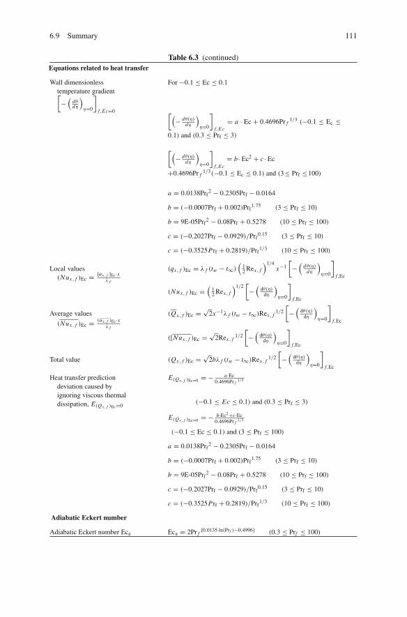
6.9 Summary 111
Table 6.3 (continued)Equations related to heat transfer
Wall dimensionlesstemperature gradient[−(
dθdη
)η=0
]
f,Ec=0
For −0.1 ≤ Ec ≤ 0.1
[(− dθ(η)
dη
)η=0
]
f,Ec= a · Ec + 0.4696Pr f
1/3 (−0.1 ≤ Ec ≤0.1) and (0.3 ≤ Prf ≤ 3)
[(− dθ(η)
dη
)η=0
]
f,Ec= b· Ec2 + c· Ec
+0.4696Pr f1/3(−0.1 ≤ Ec ≤ 0.1) and (3≤ Prf ≤100)
a = 0.0138Prf2 − 0.2305Prf − 0.0164
b = (−0.0007Prf + 0.002)Prf1.75 (3 ≤ Prf ≤ 10)
b = 9E-05Prf2 − 0.08Prf + 0.5278 (10 ≤ Prf ≤ 100)
c = (−0.2027Prf − 0.0929)/Prf0.15 (3 ≤ Prf ≤ 10)
c = (−0.3525Prf + 0.2819)/Prf1/3 (10 ≤ Prf ≤ 100)
Local values(Nux, f )Ec = [αx, f ]Ec ·x
λ f
(qx, f )Ec = λ f (tw − t∞)(
12 Rex, f
)1/4x−1[−(
dθ(η)dη
)η=0
]
f,Ec
(Nux, f )Ec =(
12 Rex, f
)1/2[−(
dθ(η)dη
)η=0
]
f,Ec
Average values
(Nux, f )Ec = (αx, f )Ec·xλ f
(Qx, f )Ec = √2x−1λ f (tw − t∞)Rex, f
1/2[−(
dθ(η)dη
)η=0
]
f,Ec
([Nux, f )Ec = √2Rex, f
1/2[−(
dθ(η)dη
)η=0
]
f,Ec
Total value (Qx, f )Ec = √2bλ f (tw − t∞)Rex, f
1/2[−(
dθ(η)dη
)η=0
]
f,Ec
Heat transfer predictiondeviation caused byignoring viscous thermaldissipation, E(Qx, f )Ec=0
E(Qx, f )Ec=0 = − a·Ec0.4696Pr f
1/3
(−0.1 ≤ Ec ≤ 0.1) and (0.3 ≤ Prf ≤ 3)
E(Qx, f )Ec=0 = − b·Ec2+c·Ec0.4696Pr f
1/3
(−0.1 ≤ Ec ≤ 0.1) and (3 ≤ Prf ≤ 100)
a = 0.0138Prf2 − 0.2305Prf − 0.0164
b = (−0.0007Prf + 0.002)Prf1.75 (3 ≤ Prf ≤ 10)
b = 9E-05Prf2 − 0.08Prf + 0.5278 (10 ≤ Prf ≤ 100)
c = (−0.2027Prf − 0.0929)/Prf0.15 (3 ≤ Prf ≤ 10)
c = (−0.3525Prf + 0.2819)/Prf1/3 (10 ≤ Prf ≤ 100)
Adiabatic Eckert number
Adiabatic Eckert number Eca Eca = 2Pr f[0.0135·ln(Prf )−0.4996] (0.3 ≤ Prf ≤ 100)

112 6 Heat Transfer of Laminar Forced Convection
6.10 Remarks
The work in this chapter is an extensive study for effect of the viscous thermal dis-sipation on heat transfer of laminar forced convection. Based on the new similarityanalysis method, a system of similarity governing mathematical model is providedfor laminar forced convection with consideration of viscous thermal dissipation andconstant physical properties for the extensive investigation.
A system of numerical solution is rigorously found out together with variationof Eckert number and average Prandtl number. With these numerical solutions, itis clear that: (i) Increasing the Eckert number causes decrease of the positive heattransfer (from the wall to flow), and causes increase of the negative heat transfer(from the flow to the wall); (ii) With increasing the Prandtl number, the effect of theviscous thermal dissipation on heat transfer will increase.
The system of key numerical solutions on wall dimensionless temperature gradi-ent are formulated with the viscous thermal dissipation and average Prandtl numberby using a curve-fitting approach, and the formulated equations are so reliable thatthey are very coincident to the related key numerical solutions. Then, combinedwith the theoretical equations on heat transfer, the simple and reliable predictionof heat transfer is realized by using these formulated equations on the wall dimen-sionless temperature gradient. Furthermore, deviation of heat transfer predicted byignoring the viscous thermal dissipation is formulated, which is used for judgementof validity of ignoring the viscous thermal dissipation in practical calculation.
The adiabatic Eckert number Eca is provided for judgement of heat flux direction,that is positive (from wall to the flow bulk) with Ec < Eca and negative (fromflow bulk to wall) with Ec > Eca. Increasing the absolute value of the increment,|Ec − Eca|, will cause increase of heat transfer no matter heat flux direction. A sys-tem of numerical solutions on the adiabatic Eckert numbers is provided and thenformulated numerically with variation of average Prandtl number. It is clear that theadiabatic Eckert number will increase at an accelerative pace with decrease of theaverage Prandtl number, especially in the region with lower Prandtl number.
6.11 Calculation Examples
Example 1 A flat plate with b = 1 m in width and x = 0.25 m in length is hor-izontally located in water flowing with wx,∞ = 1.3 m/s. The water temperatureis t∞ = 10◦C, and surface temperature of the plate is tw = 70◦C. If we ignorevariable physical properties but consider viscous thermal dissipation, please solvethe following questions:
(1) judge if the forced convection is laminar;(2) calculate the Eckert number;(3) predict heat transfer prediction deviation caused by ignoring the viscous thermal
dissipation.(4) calculate the forced convection heat transfer on the plate;(5) evaluate the adiabatic Eckert numbers Eca.
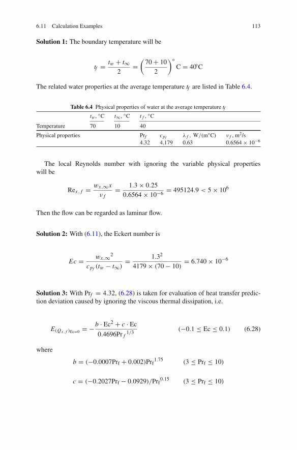
6.11 Calculation Examples 113
Solution 1: The boundary temperature will be
tf = tw + t∞2
=(
70 + 10
2
)◦C = 40◦C
The related water properties at the average temperature tf are listed in Table 6.4.
Table 6.4 Physical properties of water at the average temperature tf
tw , ◦C t∞, ◦C t f , ◦C
Temperature 70 10 40
Physical properties Prf cpf λ f , W/(m◦C) ν f , m2/s4.32 4.179 0.63 0.6564 × 10⁻⁶
The local Reynolds number with ignoring the variable physical propertieswill be
Rex, f = wx,∞x
ν f= 1.3 × 0.25
0.6564 × 10−6 = 495124.9 < 5 × 10⁶
Then the flow can be regarded as laminar flow.
Solution 2: With (6.11), the Eckert number is
Ec = wx,∞2
cpf (tw − t∞)= 1.32
4179 × (70 − 10)= 6.740 × 10⁻⁶
Solution 3: With Prf = 4.32, (6.28) is taken for evaluation of heat transfer predic-tion deviation caused by ignoring the viscous thermal dissipation, i.e.
E(Qx, f )Ec=0 = −b · Ec2 + c · Ec
0.4696Pr f1/3
(−0.1 ≤ Ec ≤ 0.1) (6.28)
where
b = (−0.0007Prf + 0.002)Prf1.75 (3 ≤ Prf ≤ 10)
c = (−0.2027Prf − 0.0929)/Prf0.15 (3 ≤ Prf ≤ 10)
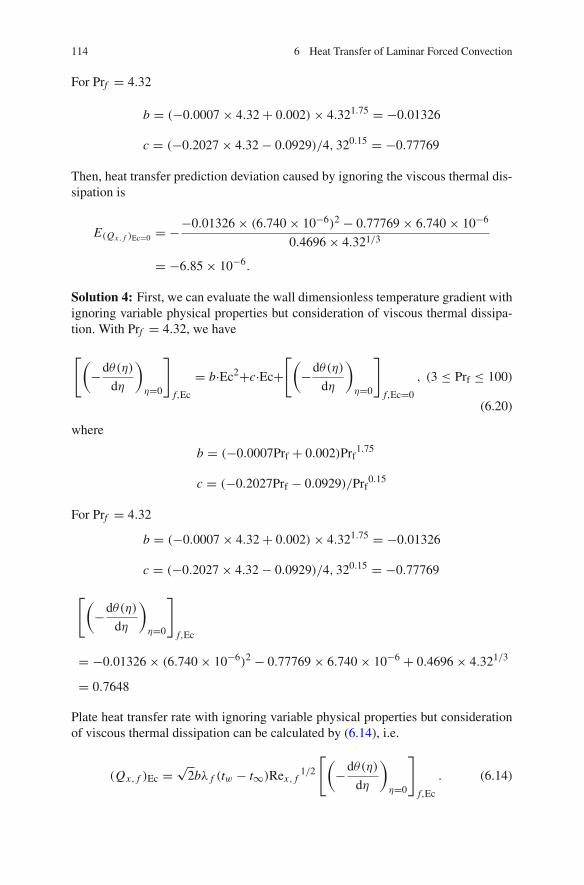
114 6 Heat Transfer of Laminar Forced Convection
For Prf = 4.32
b = (−0.0007 × 4.32 + 0.002)× 4.321.75 = −0.01326
c = (−0.2027 × 4.32 − 0.0929)/4, 320.15 = −0.77769
Then, heat transfer prediction deviation caused by ignoring the viscous thermal dis-sipation is
E(Qx, f )Ec=0 = −−0.01326 × (6.740 × 10−6)2 − 0.77769 × 6.740 × 10−6
0.4696 × 4.321/3
= −6.85 × 10⁻⁶.
Solution 4: First, we can evaluate the wall dimensionless temperature gradient withignoring variable physical properties but consideration of viscous thermal dissipa-tion. With Prf = 4.32, we have
[(−dθ(η)
dη
)
η=0
]
f,Ec
= b·Ec2+c·Ec+[(
−dθ(η)
dη
)
η=0
]
f,Ec=0
, (3 ≤ Prf ≤ 100)
(6.20)
where
b = (−0.0007Prf + 0.002)Prf1.75
c = (−0.2027Prf − 0.0929)/Prf0.15
For Prf = 4.32
b = (−0.0007 × 4.32 + 0.002)× 4.321.75 = −0.01326
c = (−0.2027 × 4.32 − 0.0929)/4, 320.15 = −0.77769
[(−dθ(η)
dη
)
η=0
]
f,Ec
= −0.01326 × (6.740 × 10−6)2 − 0.77769 × 6.740 × 10−6 + 0.4696 × 4.321/3
= 0.7648
Plate heat transfer rate with ignoring variable physical properties but considerationof viscous thermal dissipation can be calculated by (6.14), i.e.
(Qx, f )Ec = √2bλ f (tw − t∞)Rex, f
1/2
[(−dθ(η)
dη
)
η=0
]
f,Ec
. (6.14)

6.11 Calculation Examples 115
Then
(Qx, f )Ec = √2 × 1 × 0.63 × (70 − 10)× 495124.91/2 × 0.764737 = 28765.8 W
Solution 5: According to (6.29), adiabatic Eckert numbers Eca is expressed as
Eca = 2Pr f[0.0135·ln(Prf )−0.4996]
With Prf = 4.32, the adiabatic Eckert numbers Eca is
Eca = 2 × Pr f[0.0135·ln(4.32)−0.4996] = 0.99105
Example 2 Only the water flow is replaced by air flow, all other conditions are sameas those in example 1. If the ignoring variable physical properties but considerationof viscous thermal dissipation, please
(1) judge if the forced convection is laminar;(2) calculate the Eckert number;(3) predict heat transfer prediction deviation caused by ignoring the viscous thermal
dissipation.(4) calculate the forced convection heat transfer on the plate;(5) evaluate the adiabatic Eckert numbers Eca.
Solution 1: The related air properties at the average temperature tf are listed inTable 6.5.
Table 6.5 Physical properties of air at the average temperature tf
tw,◦C t∞,◦C t f ,◦C
Temperature 70 10 40
Physical properties Prf cpf λ f ,W/(m◦C) νf ,m2/s0.7 1.007 0.02726 17.20 × 10⁻⁶
The local Reynolds number with ignoring the variable physical propertieswill be
Rex, f = wx,∞x
νf= 1.3 × 0.25
17.20 × 10−6 = 18895.3 < 5 × 10⁵
Then, the flow can be regarded as laminar flow.
Solution 2: With (6.11), the Eckert number is
Ec = wx,∞2
cpf (tw − t∞)= 1.32
1007 × (70 − 10)= 2.797 × 10⁻⁵

116 6 Heat Transfer of Laminar Forced Convection
Solution 3: With Prf = 0.7, (6.27) is taken for predict heat transfer prediction devi-ation caused by ignoring the viscous thermal dissipation, i.e.
E(Qx, f )Ec=0 = − a · Ec
0.4696Pr f1/3
(−0.1 ≤ Ec ≤ 0.1) and (0.3 ≤ Prf ≤ 3) (6.27)
where
a = 0.0138Prf2 − 0.2305Prf − 0.0164
Then
a = 0.0138 × 0.72 − 0.2305 × 0.7 − 0.0164 = −0.17099
E(Qx, f )Ec=0 = −−0.17099 × 2.797 × 10−5
0.4696 × 0.71/3 = −1.147 × 10⁻⁵
Solution 4: First, we can evaluate the wall dimensionless temperature gradient withignoring variable physical properties but consideration of viscous thermal dissipa-tion. With Prf = 0.7, we have
[(−dθ(η)
dη
)
η=0
]
f,Ec
= a · Ec + 0.4696Pr f1/3 (0.3 ≤ Prf ≤ 3) (6.19)
Then,
[(−dθ(η)
dη
)
η=0
]
f,Ec
= −0.17099 × 2.797 × 10−5 + 0.4696 × 0.71/3 = 0.416955
With (6.14), the plate heat transfer rate with ignoring variable physical propertiesbut consideration of viscous thermal dissipation will be
(Qx, f )Ec = √2bλ f (tw − t∞)Rex, f
1/2
[(−dθ(η)
dη
)
η=0
]
f,Ec
(6.14)
Then,
(Qx, f )Ec = √2 × 1 × 0.02726 × (70 − 10)× 18895.31/2 × 0.416955 = 132.57 W
Solution 5: According to (6.29), adiabatic Eckert numbers Eca is expressed as
Eca = 2Pr f[0.0135·ln(Prf )−0.4996]
With Prf = 0.7, the adiabatic Eckert numbers Eca is
Eca = 2Pr f[0.0135·ln(8.13)−0.4996] = 2 × 0.7[0.0135·ln(0.7)−0.4996] = 2.394225

References 117
Exercise
1. Follow example 1, change t∞ to 30◦C, but keep all other conditions.If we ignore variable physical properties but consider viscous thermal dissipa-tion, please solve the following:
(1) judge if the forced convection is laminar;(2) calculate the Eckert number;(3) predict heat transfer prediction deviation caused by ignoring the viscous
thermal dissipation;(4) calculate the forced convection heat transfer on the plate;(5) evaluate the adiabatic Eckert numbers Eca.
References
1. H.H. Winter, Viscous dissipation in shear flows of molten polymers. Adv Heat Transfer 13,205–267 (1977).
2. H.H. Winter, Temperature induced pressure gradient in the clearance between screw flight andbarrel of a single screw extruder. Polym Eng Sci 20, 406–412 (1980)
3. V.D. Dang, Heat transfer of a power-law fluid at low Peclet number flow. J. Heat Transfer 105,542–549 (1983)
4. T. Basu, D.N. Roy, Laminar heat transfer in a tube with viscous dissipation. Int J Heat MassTransfer 28, 699–701 (1985)
5. A. Lawal, A.S. Mujumdar, The effects of viscous dissipation on heat transfer to power lawfluids in arbitrary cross-sectional ducts, Warme Stoffübertragung 27, 437–446 (1992)
6. Berardi PG, Cuccurullo G, Acierno D, Russo P. Viscous dissipation in duct flow of moltenpolymers. Proceedings of Eurotherm Seminar 46 (Pisa, Italy, July 1995), pp. 39–43
7. E. Zanchini, Effect of viscous dissipation on the asymptotic behavior of laminar forced con-vection in circular tubes. Int J Heat Mass Transfer 40, 169–178 (1997)
8. O. Aydin, Effects of viscous dissipation on the heat transfer in a forced pipe flow. Part 2:Thermally developing flow. Energy Convers Manage 46(18–19), 3091–3102 (2005)
9. O. Aydin, Effects of viscous dissipation on the heat transfer in a forced pipe flow. Part 1. Bothhydrodynamically and thermally fully developed flow, Energy Convers Manage 46, 757–769(2005)
10. E.R.G. Eckert, R.M. Drake, Analysis of Heat and Mass Transfer (McGraw-Hill, NY, 1972)11. H. Schlichting, J. Kestin, Boundary Layer Theory (McGraw-Hill, NewYork, NY 1955)

Chapter 7Heat Transfer of Gas Laminar ForcedConvection with Consideration of VariablePhysical Properties
Abstract The new similaritye analysis method is applied to develop a novelsimilarity analysis model of laminar forced convection with consideration of vari-able physical properties. It is a better alternative to the traditional Falkner-Skantype transformation for this issue. Meanwhile, an advanced approach on treat-ment of gas variable physical properties, the temperature parameter method, is firstapplied for convenient and reliable treatment of variable thermophysical proper-ties in extensive study on gas laminar forced convection. Theoretical equationson skin-friction coefficient and heat transfer with consideration of variable physi-cal properties are obtained, where only the dimensionless wall velocity and tem-perature gradients are no-given variables, respectively, both of which depend onPrandtl number, boundary temperature ratio, and gas temperature parameters. Thenumerical solutions on the dimensionless wall velocity and temperature gradientsare found out rigorously on laminar forced convection on horizontal flat plate.A system of the wall dimensionless temperature gradient is formulated by a curve-fitting method, and then a difficult point was resolved for simple and reliable predic-tion of heat transfer with consideration of variable physical properties. It is foundthat not only Prandtl number but also gas temperature parameters together with theboundary temperature ratio have significant influences on velocity and temperaturefields as well as heat transfer of gas laminar forced convection. Furthermore, the fol-lowing regulations for the effect of the variable physical properties on heat transfercoefficient are clarified: (i) Effect of the gas variable physical properties on the heattransfer coefficient are dominated by the gas temperature parameters and boundarytemperature ration; (ii) The effect of variable thermal conductivity on heat transfercoefficient is larger than that of the variable absolute viscosity, although the effectof the viscosity can never be ignored; and (iii) Increasing the boundary temperatureratio causes increase of the effect of the variable physical properties on heat transfer.
7.1 Introduction
Heat transfer of forced convection exists widely in every field of engineering prac-tice and human life, so it is important to rigorously investigate this phenomenon.On the early time, the single Blasius ordinary equation transformed from the
D.Y. Shang, Theory of Heat Transfer with Forced Convection Film Flows,Heat and Mass Transfer, DOI 10.1007/978-3-642-12581-2_7,C© Springer-Verlag Berlin Heidelberg 2011
119
120 7 Heat Transfer of Gas Laminar Forced Convection
momentum partial differential equations was applied for prediction of its veloc-ity field [1]. Pohlhausen [2] used Blasius transformation system to further calcu-late heat transfer with constant property assumption for laminar forced convectionon a horizontal flat plate. After their studies, the investigations have been donefor the effect of the variable thermophysical properties on compressible forcedboundary layer (see Schlichting [3]). For incompressible forced boundary layer,there have been some studies with consideration of variable liquid viscosity, forinstance, the studies of Ling and Dybbs [4, 5], who proposed an assumed equa-tion for approximate simulation of the viscosity of the fluid, where the viscos-ity of the fluid is an inverse linear function of temperature. Recently, Postelnicuet al. [6] extended Ling and Dybbs’ problem with an internal heat generationplaced into the fluid-saturated porous medium. However, there still has been arequirement for an extensive investigation of coupled effect of the variable phys-ical properties, such as density, thermal conductivity, and viscosity on heat transferof forced convection. In my recent book [7], the coupled effect of these variablephysical properties on heat transfer with free convection and free film flows weresystematically reported. These studies demonstrated that the variable physical prop-erties have obvious effect on free convection and frees film flows, and then cannever be ignored for reliable prediction of the related heat transfer. In view of theimportance of heat transfer of forced convection, since this Chapter, I will reportsuccessively the coupled effect of variable physical properties on heat transfer oflaminar forced convection boundary layer and force film condensation.
Here, it is necessary to mention again the subscripts for expression of ignoringthe viscous thermal dissipation. In Chaps. 5 and 6 for laminar forced convection forconsideration of constant physical properties, I gave the subscripts Ec = 0 and Ecin the related heat transfer variables for noting the cases with ignoring and consid-ering viscous thermal dissipation respectively. According to these studies and theadditional examples calculation results, it can be found that in the range of laminarforced convection the Eckert number is very small generally, and then ignoring theeffect of the viscous thermal dissipation will not cause obvious influence on lami-nar forced convection and heat transfer. Then, from now on in this book, my workwill focus on the coupled effects of variable physical properties on laminar forcedconvection and film condensation. Although the viscous thermal dissipation will notbe considered in the successive studies, the subscript Ec = 0 will never be notedanymore for saving space.
7.2 Governing Equations
7.2.1 Governing Partial Differential Equations
The physical model and coordinate system of boundary layer with two-dimensionallaminar forced convection shown in Fig. 5.1 schematically. A flat plate ishorizontally located in parallel fluid flow with its mainstream velocity wx,∞. The

7.2 Governing Equations 121
plate surface temperature is tw and the fluid bulk temperature is t∞. Then a velocityboundary layer is produced near the plate. If tw is not equal to t∞, a temperatureboundary layer will occur near the plate. We assume that the velocity boundarylayer is laminar. The only difference of the present issue from that in Chap. 5 is thatthe variable physical properties are considered here, but were never considered inChap. 5. Then if we ignore the viscous thermal dissipation, from Chap. 2 the govern-ing partial differential equations for fluid laminar forced convection boundary layerare expressed as below with consideration of these variable physical properties:
∂
∂x(ρwx )+ ∂
∂y
(ρwy) = 0, (7.1)
ρ
(wx∂wx
∂x+ wy
∂wx
∂y
)= ∂
∂y
(μ∂wx
∂y
), (7.2)
ρ
[wx∂(cpt)
∂x+ wy
∂(cpt)
∂y
]= ∂
∂y
(λ∂t
∂y
), (7.3)
with the boundary conditions
y = 0 : wx = 0, wy = 0, t = tw (7.4)
y → ∞: wx = wx,∞ (constant), t = t∞ (7.5)
Here, temperature-dependent physical properties density ρ, absolute viscosity μ,thermal conductivity λ, and specific heat cp are taken into account.
7.2.2 Similarity Transformation Variables
The similarity transformation variables used in Chap. 5 for laminar forced convec-tion without consideration of variable physical properties can be taken as those withconsideration of variable physical properties in this chapter. Of course, the averagevalue on physical properties should be changed to the related local value; and there-fore, the local Reynolds number Rex, f = wx,∞x
ν fwith the average kinetic viscosity
ν f is changed to the local Reynolds number Rex,∞ = wx,∞xν∞ with the local kinetic
viscosity ν∞. In this case, for the new similarity analysis method, a set of the relateddimensional analysis variables can be shown as follows for consideration of variablephysical properties:
η = y
x
(1
2Rex,∞
)1/2
, (7.6)
Rex,∞ = wx,∞x
ν∞, (7.7)

122 7 Heat Transfer of Gas Laminar Forced Convection
wx = wx,∞Wx (η), (7.8)
wy = wx,∞(
1
2Rex,∞
)−1/2
Wy(η), (7.9)
θ(η) = t − t∞tw − tw
, (7.10)
where η is dimensionless coordinate variable, Rex,∞ is local Reynolds number withconsideration of variable physical properties, Wx (η) and Wy(η) are dimensionlessvelocity components in x and y coordinates, respectively, and θ(η) denotes dimen-sionless temperature.
7.2.3 Similarity Transformation of the Governing PartialDifferential Equations
With (7.6), (7.7), (7.8), (7.9), and (7.10) for the dimensionless similarity variables η,Rex,∞, Wx (η), Wy(η), and θ(η), the governing partial differential equations (7.1),(7.2), and (7.3) are transformed as below respectively.
7.2.3.1 Transformation of (7.1)
Equation (7.1) is changed to the following form
ρ∂wx
∂x+ ρ
∂wy
∂y+ wx
∂ρ
∂x+ wy
∂ρ
∂y= 0. (7.1a)
With (7.8) we have
∂wx
∂x= wx,∞
dWx (η)
dη
∂η
∂x.
Where with (7.6) we have
∂η
∂x= −1
2ηx−1. (a)
Then,
∂wx
∂x= −1
2ηx−1wx,∞
dWx (η)
dη. (b)
With (7.9) we have
∂wy
∂y= wx,∞
(1
2Rex,∞
)−1/2 dWy(η)
dη
∂η
∂y,

7.2 Governing Equations 123
where
∂η
∂y= x−1
(1
2Rex,∞
)1/2
. (c)
Then
∂wy
∂y= wx,∞
dWy(η)
dηx−1. (d)
In addition,
∂ρ
∂x= dρ
dη
∂η
∂x= −1
2
dρ
dηηx−1, (e)
∂ρ
∂y= dρ
dη
∂η
∂y= dρ
dηx−1(
1
2Rex,∞
)1/2
. (f)
With (b), (d), (e), and (f), (7.1a) is changed to
ρ
[−1
2ηx−1wx,∞
dWx (η)
dη+ wx,∞
dWy(η)
dηx−1]
− 1
2
dρ
dηηx−1wx,∞Wx (η)+ dρ
dηx−1(
1
2Rex,∞
)1/2
wx,∞(
1
2Rex,∞
)−1/2
Wy(η)= 0
.
The above equation is divided by 12 x−1wx,∞, and we have
ρ
[−ηdWx (η)
dη+ 2
dWy(η)
dη
]− dρ
dηη · Wx (η)+ 2
dρ
dηWy(η) = 0.
The above equation is simplified to
− ηdWx (η)
dη+ 2
dWy(η)
dη+ 1
ρ
dρ
dη[−η · Wx (η)+ 2Wy(η)] = 0. (7.11)
7.2.3.2 Transformation of (7.2)
Equation (7.2) is changed to
ρ
(wx∂wx
∂x+ wy
∂wx
∂y
)= μ
∂2wx
∂y2+ ∂μ
∂y
∂wx
∂y. (7.2a)
With (7.8) we have
∂wx
∂y= wx,∞
dWx (η)
dη
∂η
∂y.

124 7 Heat Transfer of Gas Laminar Forced Convection
With (c), the above equation is changed to
∂wx
∂y= wx,∞
dWx (η)
dηx−1(
1
2Rex,∞
)1/2
(g)
and
∂2wx
∂y2= wx,∞
d2Wx (η)
dη2x−1(
1
2Rex,∞
)1/2∂η
∂y,
i.e.
∂2wx
∂y2 = wx,∞d2Wx (η)
dη2 x−2(
1
2Rex,∞
). (h)
Additionally,
∂μ
∂y= dμ
dηx−1(
1
2Rex,∞
)1/2
. (i)
With (7.8), (7.9), (b), (g), (h), and (i), (7.2a) is changed to
ρ
[−wx,∞Wx (η)
1
2ηx−1wx,∞
dWx (η)
dη+ wx,∞
(1
2Rex,∞
)−1/2
Wy(η) · wx,∞dWx (η)
dηx−1(
1
2Rex,∞
)1/2]
= μwx,∞d2Wx (η)
dη2x−2(
1
2Rex,∞
)+ dμ
dηx−1(
1
2Rex,∞
)1/2
wx,∞dWx (η)
dηx−1(
1
2Rex,∞
)1/2
.
The above equation is divided by 12 , and simplified to
ρ
[−wx,∞Wx (η) · ηx−1wx,∞
dWx (η)
dη+ 2wx,∞Wy(η) · wx,∞
dWx (η)
dηx−1]
= μwx,∞d2Wx (η)
dη2 x−2(Rex,∞)+ dμ
dηx−1(Rex,∞)wx,∞
dWx (η)
dηx−1
.
With definition of the local Reynolds number, the above equation is changed to
ρ
[−wx,∞Wx (η) · ηx−1wx,∞
dWx (η)
dη+ 2wx,∞Wy(η) · wx,∞
dWx (η)
dηx−1]
= μwx,∞d2Wx (η)
dη2x−2(wx,∞x
ν∞
)+ dμ
dηx−1(wx,∞x
ν∞
)wx,∞
dWx (η)
dηx−1
.
7.2 Governing Equations 125
The above equation is divided by x−1w2x,∞
μν∞ , and simplified to
ν∞ν(−ηWx (η)+ 2Wy(η))
dWx (η)
dη= d2Wx (η)
dη2+ 1
μ
dμ
dη
dWx (η)
dη. (7.12)
7.2.3.3 Transformation of (7.3)
Equation (7.3) is changed to
ρ
(wx cp
∂t
∂x+ wx t
∂cp
∂x+ wycp
∂t
∂y+ wyt
∂cp
∂y
)= λ
∂2t
∂y2+ ∂λ
∂y
∂t
∂y. (7.3a)
With (7.6), (7.10), and (a), we have
∂t
∂x= (tw − t∞)
dθ(η)
dη
∂η
∂x,
= (tw − t∞)dθ(η)
dη
(−1
2ηx−1),
= −1
2ηx−1(tw − t∞)
dθ(η)
dη. (j)
With (7.6), (7.10), and (c), we have
∂t
∂y= (tw − t∞)
dθ(η)
dη
∂η
∂y,
= (tw − t∞)dθ(η)
dηx−1(
1
2Rex,∞
)1/2
,
= x−1(
1
2Rex,∞
)1/2
(tw − t∞)dθ(η)
dη, (k)
∂2t
∂y2 = x−2(
1
2Rex,∞
)(tw − t∞)
d2θ(η)
dη2 . (l)
Similar to (e), we have
∂cp
∂x= −1
2
dcp
dηηx−1. (m)
Similar to (f), we have
∂λ
∂y= ∂λ
∂ηx−1(
1
2Rex,∞
)1/2
, (n)

126 7 Heat Transfer of Gas Laminar Forced Convection
∂cp
∂y= ∂cp
∂ηx−1(
1
2Rex,∞
)1/2
. (o)
With (7.8), (7.9), (i) to (o), (7.3a) is changed to
ρ
[wx,∞Wx (η)cp
(− 1
2ηx−1(tw − t∞) dθ(η)dη
)+ wx,∞Wx (η)t
(− 1
2ηx−1 dcpdη
)
+wx,∞(
12 Rex,∞
)−1/2Wy(η)cpx−1
(12 Rex,∞
)1/2(tw − t∞) dθ(η)
dη
+wx,∞(
12 Rex,∞
)−1/2Wy(η)t
dcpdη x−1
(12 Rex,∞
)1/2]
= λx−2(
1
2Rex,∞
)(tw − t∞)
d2θ(η)
dη2 + ∂λ
∂ηx−1(
1
2Rex,∞
)1/2
x−1(
1
2Rex,∞
)1/2
(tw − t∞)dθ(η)
dη.
The above equation is simplified to
ρ[wx,∞Wx (η)cp
(− 1
2ηx−1(tw − t∞) dθ(η)dη
)+ wx,∞Wx (η)t
(− 1
2ηx−1 dcpdη
)
+wx,∞Wy(η)cpx−1(tw − t∞) dθ(η)dη + wx,∞Wy(η)t
dcpdη x−1
]
= λx−2(
1
2Rex,∞
)(tw − t∞)
d2θ(η)
dη2+ ∂λ
∂ηx−1(
1
2Rex,∞
)x−1(tw − t∞)
dθ(η)
dη
.
With definition of Rex,∞, the above equation is changed to
ρ[wx,∞Wx (η)cp
(− 1
2ηx−1(tw − t∞) dθ(η)dη
)+ wx,∞Wx (η)t
(− 1
2ηx−1 dcpdη
)
+wx,∞Wy(η)cpx−1(tw − t∞) dθ(η)dη + wx,∞Wy(η)t
dcpdη x−1
]
= λx−2(
1
2
wx,∞x
ν∞
)(tw − t∞)
d2θ(η)
dη2 + ∂λ
∂ηx−1(
1
2
wx,∞x
ν∞
)x−1(tw − t∞)
dθ(η)
dη
.
The above equation is divided by 12(tw − t∞) cpwx,∞λ
xν∞ , and changed to
ρν∞λ
[Wx (η)
(−ηdθ(η)
dη
)+ Wx (η)
t
tw − t∞
(−η 1
cp
dcp
dη
)
+ 2Wy(η)dθ(η)
dη+ 2Wy(η)
t
tw − t∞1
cp
dcp
dη
]
= 1
cp
d2θ(η)
dη2+ 1
cp
1
λ
∂λ
∂η
dθ(η)
dη,
(7.3b)

7.2 Governing Equations 127
where
t
tw − t∞= (tw − t∞) · θ(η)+ t∞
tw − t∞= θ(η)+ t∞
tw − t∞. (p)
With (p), (7.3b) is changed to
ρν∞λ
[Wx (η)
(−ηdθ(η)
dη
)+ Wx (η)
(θ + t∞
tw − t∞
)(−η 1
cp
dcp
dη
)+ 2Wy(η)
dθ(η)
dη
+ 2Wy(η)
(θ(η)+ t∞
tw − t∞
)1
cp
dcp
dη
]= 1
cp
d2θ(η)
dη2 + 1
cp
1
λ
∂λ
∂η
dθ(η)
dη,
or
Prλ
μcpcpρν∞λ
[−ηWx (η)
dθ(η)
dη− ηWx (η)
(θ(η)+ t∞
tw − t∞
)1
cp
dcp
dη
+ 2Wy(η)dθ(η)
dη× 2Wy(η)
(θ(η)+ t∞
tw − t∞
)1
cp
dcp
dη
]= d2θ(η)
dη2 + 1
λ
∂λ
∂η
dθ(η)
dη
.
The above equation is further changed to
Prν∞ν
[−ηWx (η)
dθ(η)
dη+ 2Wy(η)
dθ(η)
dη− ηWx (η)
(θ(η)+ t∞
tw − t∞
)1
cp
dcp
dη
+ 2Wy(η)×(θ(η)+ t∞
tw − t∞
)1
cp
dcp
dη
]= d2θ(η)
dη2 + 1
λ
∂λ
∂η
dθ(η)
dη
,
i.e.
Prν∞ν
[(−ηWx (η)+ 2Wy(η))
dθ(η)
dη+ (−ηWx (η)+ 2Wy(η))
×(θ(η)+ t∞
tw − t∞
)1
cp
dcp
dη
]= d2θ(η)
dη2+ 1
λ
∂λ
∂η
dθ(η)
dη. (7.13)
For summary, governing partial differential equations (7.1), (7.2), and (7.3) havebeen transformed to the following governing ordinary differential equations:
− ηdWx (η)
dη+ 2
dWy(η)
dη+ 1
ρ
dρ
dη[−η · Wx (η)+ 2Wy(η)] = 0, (7.11)
ν∞ν(−ηWx (η)+ 2Wy(η))
∂Wx (η)
∂η= ∂2Wx (η)
∂η2+ 1
μ
∂μ
∂η
∂Wx (η)
∂η, (7.12)
128 7 Heat Transfer of Gas Laminar Forced Convection
Prν∞ν
[(−ηWx (η)+ 2Wy(η))
dθ(η)
dη+ (−ηWx (η)+ 2Wy(η))
(θ(η) + t∞
tw − t∞
)1
cp
dcp
dη= d2θ(η)
dη2 + 1
λ
∂λ
∂η
dθ(η)
dη
], (7.13)
with the boundary condition equations
η = 0 : Wx (η) = 0, Wy(η) = 0, θ(η) = 1 (7.14)
η → ∞ : Wx (η) = 1, θ(η) = 0. (7.15)
Equations (7.11), (7.12), and (7.13) are complete ordinary differential equationsof laminar forced convection. These transformed governing ordinary differentialequations are completely dimensionless because of the followings: (i) They involvedimensionless velocity components Wx (η) and Wy(η), dimensionless temperatureθ(η), as well as their dimensionless derivatives, which constitute whole unknownvariables of the governing equations; (ii) All physical properties exist in form ofthe dimensionless physical property factors, such as 1
ρdρdη , 1
μdμdη , 1
λdλdη , 1
cp
dcpdη , and
ν∞ν
as well as the temperature ratio t∞tw−t∞ . The coupled effect of the variable phys-
ical properties on laminar forced convection is dominated by these dimensionlessphysical property factors.
7.3 Treatment of Gas Variable Physical Properties
As illustrated in our research [8, 9], gas variable physical properties have significantimpacts on heat transfer of free convection and free film flows. As a result, they needto be appropriately treated to ensure accurate and reliable solution of the governingequations. In this work, I will apply this method to treat the gas variable physicalproperties for laminar forced convection. With this method, the viscosity, thermalconductivity, and specific heat are expressed as simple power law, i.e. μ ≈ T nμ ,λ ≈ T nλ , and cp ≈ cnλ
p , respectively. The absolute temperature of the gas far awayfrom the wall, T∞, can be taken as the reference temperature for forced convectionanalysis. So we assume as follows at atmospheric pressure:
μ
μ∞=(
T
T∞
)nμ, (7.16)
λ
λ∞=(
T
T∞
)nλ, (7.17)
cp
cp∞=(
T
T∞
)ncp
. (7.18)
While the change of gas density with absolute temperature at atmospheric pressureis expressed as

7.3 Treatment of Gas Variable Physical Properties 129
ρ
ρ∞=(
T
T∞
)−1
. (7.19)
Combining (16) with (19) we have
ν
ν∞=(
T
T∞
)(nμ+1)
, (7.20)
where the exponents nμ, nλ, and ncp are viscosity parameter, thermal conductivityparameter, and specific heat parameter of gas, respectively. According to the studyin [8, 9], the values of nμ, nλ, and ncp are listed in Tables 7.1 and 7.2, respectively,for different gases together with their Prandtl number Pr. These values of gas tem-perature parameters are also included in Appendix A of this book.
According to the study in [8, 9], for monatomic and diatomic gases, air, and watervapour the value of specific heat parameter ncp is so small that it can be ignored.Even for general polyatomic gases such as those listed in Table 7.2, the value of ncp
can be also ignored without any obvious deviation on heat transfer result prediction.Furthermore, with (7.10), (7.16), (7.17), (7.19), and (7.20), the related gas physi-
cal property factors in (7.11), (7.12), and (7.13) become the following ones, respec-tively with the dimensionless temperature variable θ(η) and its derivative dθ(η)/dη,boundary temperature ratio, and the related temperature parameters nμ and nλ:
1
ρ
dρ
dη= − (Tw/T∞ − 1)dθ(η)/dη
(Tw/T∞ − 1)θ(η)+ 1, (7.21)
1
μ
dμ
dη= nμ(Tw/T∞ − 1)dθ(η)/dη
(Tw/T∞ − 1)θ(η)+ 1, (7.22)
1
λ
dλ
dη= nλ(Tw/T∞ − 1)dθ(η)/dη
(Tw/T∞ − 1)θ(η)+ 1, (7.23)
Table 7.1 The value of parameters nμ and nλ with their deviations for monatomic and diatomicgases, air, and water vapour obtained according to the typical experimental data for μ and λ, citedfrom Shang and Wang [8]
Gas T0 K nμTemperaturerange K
Deviation% nλ
Temperaturerange K
Deviation% Pr
Ar 273 0.72 220–1500 ±3 0.73 210–1500 ±4 0.622He 273 0.66 273–873 ±1 0.725 273–873 ±0.3 0.675H2 273 0.68 80–1000 ±2 0.8 220–700 ±1 0.68Air 273 0.68 220–1400 ±3 0.81 220–1000 ±2.5 0.7CO 273 0.71 230–1500 ±2 0.83 220–600 ±2 0.72N2 273 0.67 220–1500 ±3 0.76 220–1200 ±3 0.71O2 273 0.694 230–2000 ±2 0.86 220–600 ±2 0.733Water
Vapour380 1.04 380–1500 ±4 1.185 380–800 ±0.3 1
Note: The value of specific heat parameter ncp is so small for monatomic and diatomic gases, air,and water vapour that it is omitted

130 7 Heat Transfer of Gas Laminar Forced Convection
Tabl
e7.
2T
heva
lues
ofte
mpe
ratu
repa
ram
eter
sn λ
,nμ
,and
n cp
with
thei
rde
viat
ions
for
poly
atom
icga
ses
obta
ined
acco
rdin
gto
the
expe
rim
enta
ldat
a,ci
ted
from
Shan
gan
dW
ang
[9]
Gas
T 0K
n μTe
mpe
ratu
reR
ange
KD
evia
tion
%n λ
Tem
pera
ture
rang
eK
Dev
iatio
n%
n cp
Tem
pera
ture
rang
eK
Dev
iatio
n%
Pr
Gas m
ixtu
re27
30.
7527
3–11
73±3
1.02
273–
1473
±10.
134
273–
1473
±2.5
0.63
CO
227
30.
8822
0–70
0±2
1.3
220–
720
±20.
3423
0–81
0±1
0.73
CH
427
30.
7822
0–10
00±3
1.29
230–
1000
±3.6
0.53
427
3–10
33±4.2
0.74
CC
l 427
30.
912
270–
500
±11.
2926
0–40
0±1
0.28
270–
700
±20.
8SO
227
30.
9120
0–12
50±4
1.32
325
0–90
0±4.5
0.25
727
3–12
00±3
0.81
H2S
273
127
0–50
0±1
1.29
260–
400
±10.
1823
0–70
0±2
0.85
NH
327
31.
0422
0–10
00±1
1.37
525
0–90
0±2
0.34
230–
1033
±0.3
60.
87N
ote:
(1)
n cp
issp
ecifi
che
atpa
ram
eter
,and
acco
rdin
gto
the
stud
yin
[9],
for
gene
ralp
olya
tom
icga
ses
itca
nbe
igno
red
with
outa
nyob
viou
sde
viat
ion
onhe
attr
ansf
erre
sults
.(2)
Not
e:co
mpo
nent
ofth
ega
sm
ixtu
re:C
O2
=0.
13,N
2=
0.76
,and
wat
erva
pour
=0.
11

7.4 Velocity and Temperature Fields 131
1
cp
dcp
dη= ncp (Tw/T∞ − 1)dθ(η)/dη
(Tw/T∞ − 1)θ(η)+ 1, (7.24)
ν∞ν
= [(Tw/T∞ − 1)θ(η)+ 1]−(nμ+1), (7.25)
Pr = Pr∞[(Tw/T∞ − 1)θ(η)+ 1]nμ−nλ+ncp . (7.26)
The Prandtl number is defined as Pr = μcp/λ. Strictly speaking, Pr should alsodepend on temperature, and described as (7.26). However, generally the variationof Prandtl number of gas is slight that it can be taken as the constant shown as inTables 7.1 and 7.2.
With the above dimensionless expressions for the dimensionless physical factors1ρ
dρdη , 1
μdμdη , 1
λdλdη , 1
cp
dcpdη , and ν∞
ν, the ordinary governing equations (7.11), (7.12),
and (7.13) can be solved numerically with the related temperature parameters nμand nλ, as well as the boundary temperature ratio Tw/T∞.
7.4 Velocity and Temperature Fields
It is mentioned according to the study in [8] and [9] that for monatomic and diatomicgases, air, and water vapour, the specific heat parameter ncp can be regarded as zerodue to its very small value, while for general polyatomic gases ncp can also be omit-ted, which will not cause any obvious deviation on heat transfer result prediction.
Since the physical properties vary with temperature, the governing equa-tions (7.11), (7.11), and (7.13) are coupled each other. They are solved by a shootingmethod with fifth-order Runge-Kutta integration with the boundary equations (7.14)and (7.15). For solving the nonlinear problem, a variable mesh approach is appliedto the numerical procedure. In this present work, forced convection for some gases istaken as example for numerical calculation. A system of accurate numerical resultsof the velocity and temperature fields is obtained as follows.
Since the governing equations of laminar forced convection are coupled eachother for consideration of gas variable physical properties, both the velocity and thetemperature fields depend on Prandtl number. In addition, they depend on the tem-perature boundary conditions and gas temperature parameters. The numerical resultsfor the dimensionless velocity component Wx (η) and dimensionless temperatureθ(η) of air, a gas mixture, water vapour, and N H3 laminar forced convection on ahorizontal flat plate are obtained, and plotted in Figs. 7.1, 7.2, 7.3, and 7.4, respec-tively. It is really seen that not only Prandtl number but also temperature parametersnμ and nλ and the boundary temperature ratio Tw
T∞ influence the velocity and tem-perature fields of laminar forced convection. Especially, the effect of the boundarytemperature ratio Tw
T∞ on the velocity and temperature fields of gas laminar forced
convection is even obvious. While increasing the boundary temperature ratio TwT∞
will cause increase of the momentum and temperature boundary layer thicknesses.Furthermore, increasing the overall temperature parameter (nμλ = 0.45nμ+0.55nλ)

132 7 Heat Transfer of Gas Laminar Forced Convection
0
0.2
0.4
0.6
0.8
1
1
11
Wx
(η)
0 2 4 6 8η
(a)
Pr = 0.7, nµ = 0.68, nλ = 0.81, nµλ = 0.7515air forced convection
0
0.2
0.4
0.6
0.8
1
0 2 4 6 8η
1
11
θ (η
)
(b)
Pr = 0.7, nµ = 0.68, nλ = 0.81, nµλ = 0.7515air forced convection
Fig. 7.1 Velocity and temperature profiles of air laminar forced convection on a horizontal platewith variation of the boundary temperature ratio Tw
T∞Note: 1. Lines 1 to 11 for Tw
T∞ = 0.3, 0.5, 0.75, 0.9, → 1, 1.1, 1.25, 1.5, 2, 2.5 and 3; 2. (a) denotesvelocity profile, and (b) denotes temperature profile
1
11
1
11
0
0.2
0.4
0.6
0.8
1
0 2 4 6 8η
(a)
0
0.2
0.4
0.6
0.8
1
0 2 4 6 8η
(b)
Pr = 0.63, nµ = 0.75, nλ = 1.02, nµλ = 0.8985a gas mixture forced convection
Pr = 0.63, nµ = 0.75, nλ = 1.02, nµλ = 0.8985a gas mixture forced convection
Wx
(η)
θ (η
)
Fig. 7.2 Velocity and temperature profiles of a gas mixture laminar forced convection on ahorizontal plate with variation of the boundary temperature ratio Tw
T∞Note: 1. Lines 1 to 11: for Tw
T∞ = 0.3, 0.5, 0.75, 0.9, → 1, 1.1, 1.25, 1.5, 2, 2.5, and 3; 2. Compo-nents of the gas mixture are CO2 = 0.13, water vapour = 0.11 and N2 = 0.76 with Pr = 0.63,nμ = 0.75 and nλ = 1.02; 3. (a) denotes velocity profile, and (b) denotes temperature profile
1
11
1
11
(b)
0
0.2
0.4
0.6
0.8
1
0 2 4 6 8η
0 2 4 6 8η
(a)
0
0.2
0.4
0.6
0.8
1
Pr = 1, nµ = 1.04, nλ = 0.185, nµλ = 1.11975water vapour forced convection
Pr = 1, nµ = 1.04, nλ = 0.185, nµλ = 1.11975water vapour forced convection
θ (η)
Wx
(η)
Fig. 7.3 Velocity and temperature profiles of water vapour laminar forced convection on ahorizontal plate with variation of the boundary temperature ratio Tw
T∞Note: 1. Lines 1 to 11: for Tw
T∞ = 0.3, 0.5, 0.75, 0.9, → 1, 1.1, 1.25, 1.5, 2, 2.5, and 3; 2. (a) denotesvelocity profile, and (b) denotes temperature profile
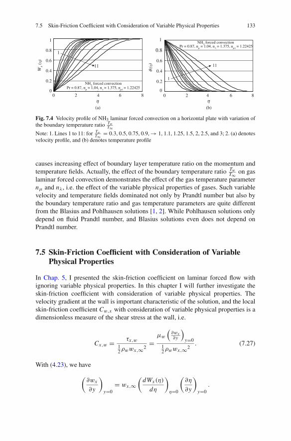
7.5 Skin-Friction Coefficient with Consideration of Variable Physical Properties 133
1
11
0
0.2
0.4
0.6
0.8
1
0 2 4 6 8η(a)
1
11
0
0.2
0.4
0.6
0.8
1
0 2 4 6 8η(b)
Pr = 0.87, nµ = 1.04, nλ = 1.375, nµλ = 1.22425NH3 forced convection
Pr = 0.87, nµ = 1.04, nλ = 1.375, nµλ = 1.22425NH3 forced convection
Wx
(η)
θ (η
)
Fig. 7.4 Velocity profile of NH3 laminar forced convection on a horizontal plate with variation ofthe boundary temperature ratio Tw
T∞Note: 1. Lines 1 to 11: for Tw
T∞ = 0.3, 0.5, 0.75, 0.9, → 1, 1.1, 1.25, 1.5, 2, 2.5, and 3; 2. (a) denotesvelocity profile, and (b) denotes temperature profile
causes increasing effect of boundary layer temperature ratio on the momentum andtemperature fields. Actually, the effect of the boundary temperature ratio Tw
T∞ on gaslaminar forced convection demonstrates the effect of the gas temperature parameternμ and nλ, i.e. the effect of the variable physical properties of gases. Such variablevelocity and temperature fields dominated not only by Prandtl number but also bythe boundary temperature ratio and gas temperature parameters are quite differentfrom the Blasius and Pohlhausen solutions [1, 2]. While Pohlhausen solutions onlydepend on fluid Prandtl number, and Blasius solutions even does not depend onPrandtl number.
7.5 Skin-Friction Coefficient with Consideration of VariablePhysical Properties
In Chap. 5, I presented the skin-friction coefficient on laminar forced flow withignoring variable physical properties. In this chapter I will further investigate theskin-friction coefficient with consideration of variable physical properties. Thevelocity gradient at the wall is important characteristic of the solution, and the localskin-friction coefficient Cw,x with consideration of variable physical properties is adimensionless measure of the shear stress at the wall, i.e.
Cx,w = τx,w12ρwwx,∞2
=μw
(∂wx∂y
)y=0
12ρwwx,∞2
. (7.27)
With (4.23), we have
(∂wx
∂y
)
y=0= wx,∞
(dWx (η)
dη
)
η=0
(∂η
∂y
)
y=0.

134 7 Heat Transfer of Gas Laminar Forced Convection
With (4.12), we have
(∂η
∂y
)
y=0= x−1
(1
2Rex,∞
)1/2
.
Then
(∂wx
∂y
)
y=0= x−1
(1
2Rex,∞
)1/2
wx,∞(
dWx (η)
dη
)
η=0.
Therefore, the local skin-friction coefficient Cm,x is expressed as
Cx,w =μwx−1
(12 Rex,∞
)1/2wx,∞
(dWx (η)
dη
)η=0
12ρwwx,∞2
= √2ν∞ν∞
νw
xwx,∞(Rex,∞)1/2
(dWx (η)
dη
)
η=0
= √2νw
ν∞(Rex,∞)−1/2
(dWx (η)
dη
)
η=0
(7.28)
It should be indicated that the numerical solution(
dWx (η)dη
)η=0
here for considera-
tion of variable physical properties is different from that in Chap. 5 for ignoring the
variable physical properties. The former numerical solution(
dWx (η)dη
)η=0
is variable
with the boundary temperature ratio and gas temperature parameters.The average skin friction coefficient with consideration of variable physical prop-
erties from x = 0 to x is described as
Cx,w = 1
x
∫ x
0Cx,wdx
= √2
1
x
∫ x
0
νw
ν∞(Rex,∞)−1/2
(dWx (η)
dη
)
η=0dx
= 2 × √2νw
ν∞(Rex,∞)−1/2
(dWx (η)
dη
)
η=0
(7.29)
For evaluation of the Skin-friction coefficient with consideration of variable physi-cal properties, the numerical solutions on the wall dimensionless velocity gradient(
dWx (η)dη
)η=0
are plotted in Fig. 7.5, and listed in Table 7.3 for different gas laminar
forced convection on a horizontal flat plate. It is seen that(
dWx (η)dη
)η=0
depends on
Prandtl number Pr, gas temperature parameters nμ and nλ, as well as the bound-ary temperature ratio Tw/T∞. Especially, with increasing the boundary temperature
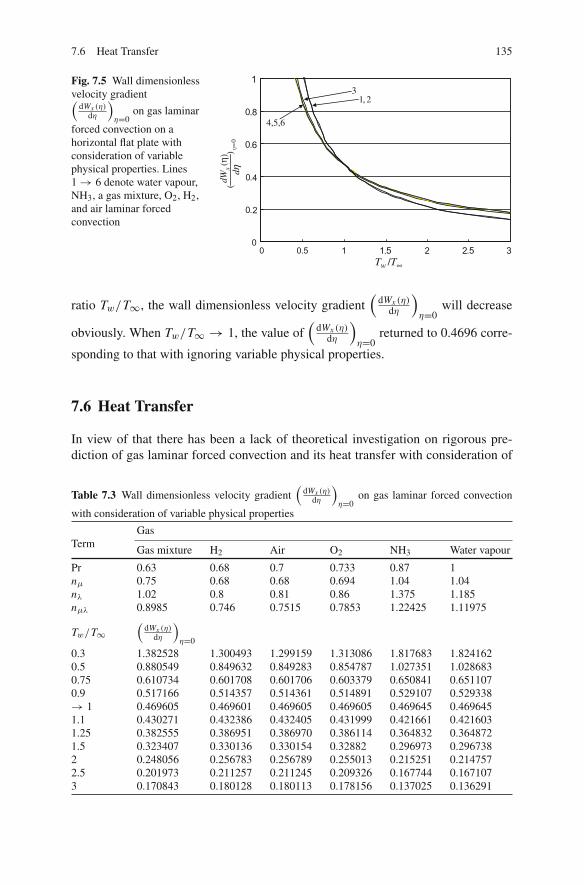
7.6 Heat Transfer 135
Fig. 7.5 Wall dimensionlessvelocity gradient(
dWx (η)dη
)η=0
on gas laminar
forced convection on ahorizontal flat plate withconsideration of variablephysical properties. Lines1 → 6 denote water vapour,NH3, a gas mixture, O2, H2,and air laminar forcedconvection
Tw /T∞
3,1 2
4,5,6
) η =
0(
ηddW
x (η
)
ratio Tw/T∞, the wall dimensionless velocity gradient(
dWx (η)dη
)η=0
will decrease
obviously. When Tw/T∞ → 1, the value of(
dWx (η)dη
)η=0
returned to 0.4696 corre-
sponding to that with ignoring variable physical properties.
7.6 Heat Transfer
In view of that there has been a lack of theoretical investigation on rigorous pre-diction of gas laminar forced convection and its heat transfer with consideration of
Table 7.3 Wall dimensionless velocity gradient(
dWx (η)dη
)η=0
on gas laminar forced convection
with consideration of variable physical properties
TermGas
Gas mixture H2 Air O2 NH3 Water vapour
Pr 0.63 0.68 0.7 0.733 0.87 1nμ 0.75 0.68 0.68 0.694 1.04 1.04nλ 1.02 0.8 0.81 0.86 1.375 1.185nμλ 0.8985 0.746 0.7515 0.7853 1.22425 1.11975
Tw/T∞(
dWx (η)dη
)η=0
0.3 1.382528 1.300493 1.299159 1.313086 1.817683 1.8241620.5 0.880549 0.849632 0.849283 0.854787 1.027351 1.0286830.75 0.610734 0.601708 0.601706 0.603379 0.650841 0.6511070.9 0.517166 0.514357 0.514361 0.514891 0.529107 0.529338→ 1 0.469605 0.469601 0.469605 0.469605 0.469645 0.4696451.1 0.430271 0.432386 0.432405 0.431999 0.421661 0.4216031.25 0.382555 0.386951 0.386970 0.386114 0.364832 0.3648721.5 0.323407 0.330136 0.330154 0.32882 0.296973 0.2967382 0.248056 0.256783 0.256789 0.255013 0.215251 0.2147572.5 0.201973 0.211257 0.211245 0.209326 0.167744 0.1671073 0.170843 0.180128 0.180113 0.178156 0.137025 0.136291

136 7 Heat Transfer of Gas Laminar Forced Convection
variable thermophysical properties due to its complexity, such difficult point will beaddressed here in this work.
7.6.1 Heat Transfer Analysis
The heat transfer analysis on laminar forced convection boundary layer withconsideration of variable physical properties is done as follows.
The local heat transfer rate qx,w at position x per unit area from the surface ofthe plate to the fluid with consideration of variable physical properties and ignoringviscous thermal dissipation is calculated by Fourier’s law as qx,w = −λw( ∂t
∂y )y=0.While, with (k) we have
−(∂t
∂y
)
y=0= x−1
(1
2Rex,∞
)1/2
(tw − t∞)(
−dθ(η)
dη
)
η=0.
Then,
qx,w = λw(tw − t∞)(
1
2Rex,∞
)1/2
x−1(
−dθ(η)
dη
)
η=0, (7.30)
where(− dθ(η)
dη
)η=0
is wall dimensionless temperature gradient with consideration
of variable physical properties.The local heat transfer coefficient αx,w , defined as qx,w = αx,w(tw − t∞), will
be given by
αx,w = λw
(1
2Rex,∞
)1/2
x−1(
−dθ(η)
dη
)
η=0. (7.31)
The local Nusselt number defined by Nux,w = αx,w ·xλw
will be
Nux,w =(
1
2Rex,∞
)1/2 (−dθ(η)
dη
)
η=0. (7.32)
Total heat transfer rate for position x = 0 to x with width of b on the plate is aintegration Qx,w = ∫∫
Aqx,wdA = ∫ x
0 qx,wb dx , and hence
Qx,w = 2bλw(tw − t∞)(
1
2Rex,∞
)1/2 (−dθ(η)
dη
)
η=0. (7.33)
The average heat transfer rate defined as Qx,w = Qx,wb×x is
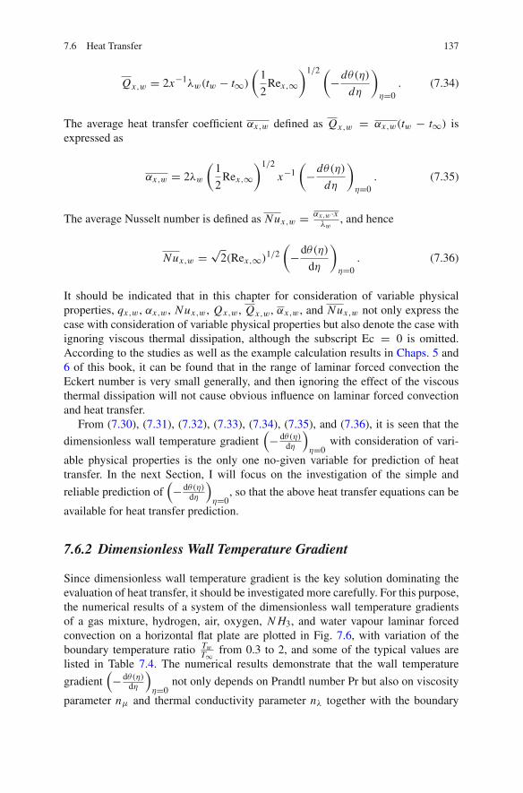
7.6 Heat Transfer 137
Qx,w = 2x−1λw(tw − t∞)(
1
2Rex,∞
)1/2 (−dθ(η)
dη
)
η=0. (7.34)
The average heat transfer coefficient αx,w defined as Qx,w = αx,w(tw − t∞) isexpressed as
αx,w = 2λw
(1
2Rex,∞
)1/2
x−1(
−dθ(η)
dη
)
η=0. (7.35)
The average Nusselt number is defined as Nux,w = αx,w ·xλw
, and hence
Nux,w = √2(Rex,∞)1/2
(−dθ(η)
dη
)
η=0. (7.36)
It should be indicated that in this chapter for consideration of variable physicalproperties, qx,w, αx,w, Nux,w, Qx,w, Qx,w, αx,w, and Nux,w not only express thecase with consideration of variable physical properties but also denote the case withignoring viscous thermal dissipation, although the subscript Ec = 0 is omitted.According to the studies as well as the example calculation results in Chaps. 5 and6 of this book, it can be found that in the range of laminar forced convection theEckert number is very small generally, and then ignoring the effect of the viscousthermal dissipation will not cause obvious influence on laminar forced convectionand heat transfer.
From (7.30), (7.31), (7.32), (7.33), (7.34), (7.35), and (7.36), it is seen that the
dimensionless wall temperature gradient(− dθ(η)
dη
)η=0
with consideration of vari-
able physical properties is the only one no-given variable for prediction of heattransfer. In the next Section, I will focus on the investigation of the simple and
reliable prediction of(− dθ(η)
dη
)η=0
, so that the above heat transfer equations can be
available for heat transfer prediction.
7.6.2 Dimensionless Wall Temperature Gradient
Since dimensionless wall temperature gradient is the key solution dominating theevaluation of heat transfer, it should be investigated more carefully. For this purpose,the numerical results of a system of the dimensionless wall temperature gradientsof a gas mixture, hydrogen, air, oxygen, N H3, and water vapour laminar forcedconvection on a horizontal flat plate are plotted in Fig. 7.6, with variation of theboundary temperature ratio Tw
T∞ from 0.3 to 2, and some of the typical values arelisted in Table 7.4. The numerical results demonstrate that the wall temperature
gradient(− dθ(η)
dη
)η=0
not only depends on Prandtl number Pr but also on viscosity
parameter nμ and thermal conductivity parameter nλ together with the boundary

138 7 Heat Transfer of Gas Laminar Forced Convection
0
0.5
1
1.5
2
0 0.5 1 1.5 2
gas mixturehydrogenairoxygenammoniawater vapour
Tw / T∞
) η =
0(
dηdθ
(η)
Fig. 7.6 Numerical results on wall temperature gradient(− dθ(η)
dη
)η=0
of laminar forced convec-
tion on the horizontal plate with consideration of variable physical properties
temperature ratio Tw/T∞. Decreasing the boundary temperature ratio TwT∞ will cause
increase of the wall temperature gradient(−dθ(η)
dη
)η=0
in accelerative pace. In addi-
tion, different gas convection with different Prandtl numbers and overall temperatureparameters has different curve of the wall temperature gradient. All these demon-strate the effect of the variable physical properties.
It is also found that only in the case TwT∞ → 1 the calculated results on the wall
temperature gradient(−dθ(η)
dη
)μ=0
here is identical to that without consideration
of variable physical properties shown in Chap. 5. It is because only in the caseTwT∞ → 1, the physical properties of the boundary layer can be regarded as constant.
By using a curve-fitting approach, the following equations of(− dθ(η)
dη
)η=0
are
obtained from its system of numerical results.
(−dθ(η)
dη
)=[(
−dθ(η)
dη
)
μ=0
]
Tw/T∞→1
· ( TwT∞
)−m, (7.37)
where
[(− dθ(η)
dη
)η=0
]
Tw/T∞→1is the reference wall dimensionless temperature
gradient with Tw/T∞ → 1 equivalent to the Pohlhausen equation [2], i.e.
[(−dθ(η)
dη
)
η=0
]
Tw/T∞→1
= 0.4696 Pr f1/3. (0.3 ≤ Pr ≤ 1) (7.38)

7.6 Heat Transfer 139
Table 7.4 Wall temperature gradient(− dθ(η)
dη
)η=0
of laminar forced convection on the horizontal
plate with consideration of variable physical properties. A: numerical results; B: predicted resultsby (7.39); C: predicted deviation
Gas Gas mixture H2 Air O2 N H3 Water vapour
Pr 0.63 0.68 0.7 0.733 0.87 1nμ 0.75 0.68 0.68 0.694 1.04 1.04nλ 1.02 0.8 0.81 0.86 1.375 1.185
Tw/T∞(− dθ(η)
dη
)η=0
0.3 A 1.426838 1.232269 1.253236 1.322974 2.217698 2.027272B 1.418567 1.246733 1.265876 1.330267 2.197733 2.070775C −0.0058 0.0117 0.0101 0.0055 −0.00903 0.0215
0.5 A 0.829365 0.774664 0.785671 0.815515 1.116327 1.088393B 0.831311 0.780136 0.790243 0.818456 1.119558 1.103374C 0.0023 0.0071 0.0058 0.0036 0.0029 0.0138
0.75 A 0.539962 0.534171 0.540901 0.554359 0.652639 0.665542B 0.543934 0.537726 0.543671 0.556622 0.655445 0.669429C 0.0074 0.0067 0.0051 0.0041 0.0043 0.0058
0.9 A 0.445409 0.451519 0.456614 0.465518 0.513033 0.533474B 0.449480 0.454875 0.459516 0.468027 0.515212 0.534713C 0.0091 0.0074 0.0064 0.0054 0.0042 0.0023
→ 1 A 0.398737 0.409666 0.413982 0.420815 0.447221 0.469645B 0.402570 0.412950 0.416960 0.423412 0.448299 0.469600C 0.0096 0.0080 0.0072 0.0062 0.0024 −0.0001
1.1 A 0.360705 0.375176 0.378990 0.384211 0.395269 0.418749B 0.364764 0.378133 0.381659 0.386660 0.397157 0.419043C 0.0113 0.0079 0.0070 0.0064 0.0048 0.0007
1.25 A 0.315595 0.333396 0.336543 0.340007 0.335059 0.359249B 0.319571 0.335999 0.338960 0.342328 0.337603 0.359674C 0.0126 0.0078 0.0072 0.0068 0.0076 0.0012
1.5 A 0.261011 0.281755 0.284165 0.285725 0.265436 0.288754B 0.264629 0.283898 0.286192 0.287747 0.267779 0.289253C 0.0139 0.0076 0.0071 0.0071 0.0088 0.0017
2 A 0.194046 0.216157 0.217738 0.217385 0.185277 0.205496B 0.19650 0.217621 0.219127 0.218771 0.185778 0.205098C 0.0126 0.0068 0.0064 0.0064 0.0027 −0.0019
2.5 A 0.1545 0.176127 0.177196 0.17607 0.140552 0.15805B 0.155987 0.177069 0.178136 0.176876 0.139905 0.157088C 0.0096 0.0053 0.0053 0.0046 −0.0046 −0.0061
3 A 0.128883 0.149113 0.149969 0.148376 0.112553 0.127796B 0.129169 0.149612 0.150404 0.148674 0.110969 0.126331C 0.0022 0.0033 0.0029 0.0020 −0.0141 −0.0115

140 7 Heat Transfer of Gas Laminar Forced Convection
Then
(−dθ(η)
dη
)
η=0= 0.4696 Pr f
1/3 · ( TwT∞
)−m, (7.39)
with
m = 0.8419nμλ + 0.2897 (0.3 ≤ Tw/T∞ ≤ 1)
m = 0.725nμλ + 0.3833 (1 ≤ Tw/T∞ ≤ 3)
Here, the overall temperature parameter nμλ is expressed by a weighted sum ofnμ and nλ, as given by
nμλ = 0.45nμ + 0.55nλ.
From (7.39) and the equations with the overall temperature parameter, the fol-lowing effect of the overall temperature parameter on the wall dimensionless tem-perature gradient is found: (1) For 0.3 ≤ Tw/T∞ ≤ 1, the wall dimensionless tem-perature gradient will increase with increasing overall temperature parameter; (2)for 1 ≤ Tw/T∞ ≤ 3, the wall dimensionless temperature gradient will decreasewith increasing overall temperature parameter. A system of the wall dimensionless
temperature gradients(− dθ(η)
dη
)η=0
of laminar forced convection of a gas mix-
ture, hydrogen, air, oxygen, N H3, and water vapour on a horizontal flat plate areevaluated by using (7.38) for different boundary temperature ratio Tw
T∞ , and listedin Table 7.4 with their evaluated deviation. It is seen that the evaluated values of−(
dθ(η)dη
)η=0
are very well coincident to the related numerical solutions.
7.6.3 Prediction Equations on Heat Transfer
With (7.39), (7.30) to (7.36) are available for prediction of heat transfer. For exam-ple, (7.33) and (7.36) will become the following corresponding equations for simpleand reliable prediction of heat transfer rate and average Nusselt number for laminargas forced convection on horizontal flat plate for consideration of coupled effects ofvariable physical properties:
Qx,w = 0.664bλw(tw − t∞)Rex,∞1/2Pr f1/3(
TwT∞
)−m
, (0.3 ≤ Pr ≤ 1) (7.40)
Nux,w = 0.664Rex,∞1/2Pr f1/3(
TwT∞
)−m
, (0.3 ≤ Pr ≤ 1) (7.41)
with
7.7 Remarks 141
m = 0.8419nμλ + 0.2897 (0.3 ≤ Tw/T∞ ≤ 1)
m = 0.725nμλ + 0.3833 (1 ≤ Tw/T∞ ≤ 3)
nμλ = 0.45nμ + 0.55nλ.
Equations (7.40) and (7.41) are used for prediction of heat transfer result of gas lam-inar forced convection on a horizontal flat plate with consideration of the coupledeffect of variable thermophysical properties. Obviously, the accuracy of (7.40) and(7.41), dependent on accuracy of reliable equation (7.39), is reliable for practicalprediction.
7.7 Remarks
A set of dimensionless similarity mathematical models of gas laminar forced con-vection with consideration of variable physical properties is developed by the newsimilarity analysis method. With this new similarity analysis method, the two-dimensional velocity components are directly transformed to the related dimension-less velocity components, which leads to a convenience for dealing with the variablephysical properties.
The advanced method, viz. the temperature parameter method for treatment ofgas variable physical properties, is first applied in extensive study on gas laminarforced convection. With this method a simple power law is applied to treat thevariations of density, viscosity, specific heat, and thermal conductivity of gases withtemperature parameters, conveniently and reliably. However, for general gas laminarconvection, the variation of specific heat with temperature can be ignored withoutany obvious deviation caused on heat transfer results, then the variable physicalproperties, which have significant effect on heat transfer, are density, thermal con-ductivity, and viscosity.
Based on the present new similarity analysis method, the equation on skin-friction coefficient for laminar forced convection is derived for consideration ofvariable physical properties. In the equation on the skin-friction coefficient, thewall dimensionless velocity component gradient as the dominating variable is theonly no-given variable which is dependent on variable physical properties. However,the wall dimensionless velocity component gradient is a constant with ignoring thevariable physical properties.
Based on the present new similarity analysis method, the theoretical equations onheat transfer are obtained through heat transfer analysis. In the theoretical equationson heat transfer, the wall dimensionless temperature gradient exists as only oneno-given variable. The wall dimensionless temperature gradient depends on Prandtlnumber Pr, boundary temperature ratio, and the temperature parameters nμ and nλfor gas laminar forced convection for consideration of variable physical properties.A system of numerical solutions of wall dimensionless temperature gradient for gaslaminar forced convection on a horizontal flat plate is formulated by a curve-fittingapproach. With the formulated equation of wall dimensionless temperature gradient,

142 7 Heat Transfer of Gas Laminar Forced Convection
the theoretical equations on heat transfer become available for simple and reliableprediction of heat transfer.
It is found that not only Prandtl number but also the temperature parameterstogether with the boundary temperature ratio have significant influences on veloc-ity and temperature fields, as well as heat transfer of gas forced convection. Theseinfluences are actually caused by the variable physical properties. Increasing thegas temperature parameters will cause decrease of heat transfer coefficient when theboundary temperature ratio is larger than unity, and cause increase of heat transfercoefficient when the boundary temperature ratio is less than the unity. The effect ofthe variable thermal conductivity on the heat transfer coefficient is slightly largerthan that of the variable viscosity. With decreasing the boundary layer tempera-ture ratio, the heat transfer coefficient will increase at an accelerative pace. Onlyin the special case when the boundary temperature ratio tends to unity, the resultof wall dimensionless temperature gradient is identical to that for ignoring thevariable physical properties. The traditional Blasius solutions on velocity field andPohlhausen equation on heat transfer are only the special cases for consideration thevariable physical properties.
7.8 Calculation Examples
Example 1 A flat plate with b = 1 m in width and x = 0.5 m in length is horizontallylocated in air flowing with the velocity wx,∞ = 7.5 m/s. The surface temperatureof the plate is tw = 427◦C, and air temperature is t∞ = 27◦C. Please solve thefollowings questions:
(1) evaluate the related local Reynolds numbers for determination of the flow types;(2) calculate the related Eckert numbers;(3) determine the related heat transfer prediction deviation caused by ignoring the
viscous thermal dissipation;(4) calculate the related heat transfer results with consideration of coupled effect of
the variable physical properties;(5) evaluate the prediction deviation of heat transfer caused by ignoring the variable
physical properties.
Solution 1: t f = tw+t∞2 = 427+27
2 = 227◦C, and tw − t∞ = 427 − 27 = 400◦C.Then, the related physical properties for air are obtained and listed in Table 7.5.
For ignoring variable physical properties, related local Reynolds number isdescribed with
Rex, f = wx,∞x
ν f= 7.5 × 0.5
38.785 × 10−6= 96686.86 < 5 × 10⁵. Then the flow is
regarded as laminar.
Solution 2: The Eckert number is evaluated as
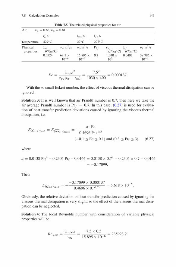
7.8 Calculation Examples 143
Table 7.5 The related physical properties for air
Air, nμ = 0.68, nμ = 0.81
Temperature
t ′wK t∞,K t f ,K
427◦C 27◦C 227◦C
Physicalproperties
λwW/(m◦C)
νw m2/s ν∞m2/s Pr f cp f
kJ/(kg◦C)λ fW/(m◦C)
ν f m2/s
0.0524 68.1 ×10⁻⁶
15.895 ×10⁻⁶
0.7 1.030 ×10³
0.0407 38.785 ×10⁻⁶
Ec = wx,∞2
cp f (tw − t∞)= 7.52
1030 × 400= 0.000137.
With the so small Eckert number, the effect of viscous thermal dissipation can beignored.
Solution 3: It is well known that air Prandtl number is 0.7, then here we take theair average Prandtl number is Pr f = 0.7. In this case, (6.27) is used for evalua-tion of heat transfer prediction deviations caused by ignoring the viscous thermaldissipation, i.e.
E(Qx, f )Ec=0 = E(Nux, f )Ec=0= − a · Ec
0.4696 Pr f1/3
(−0.1 ≤ Ec ≤ 0.1) and (0.3 ≤ Prf ≤ 3) (6.27)
where
a = 0.0138 Prf2 − 0.2305 Prf − 0.0164 = 0.0138 × 0.72 − 0.2305 × 0.7 − 0.0164
= −0.17099.
Then
E(Qx, f )Ec=0 = −−0.17099 × 0.000137
0.4696 × 0.71/3= 5.618 × 10⁻⁵.
Obviously, the relative deviation on heat transfer prediction caused by ignoring theviscous thermal dissipation is very slight, so the effect of the viscous thermal dissi-pation can be neglected.
Solution 4: The local Reynolds number with consideration of variable physicalproperties will be
Rex,∞ = wx,∞x
ν∞= 7.5 × 0.5
15.895 × 10−6= 235923.2.
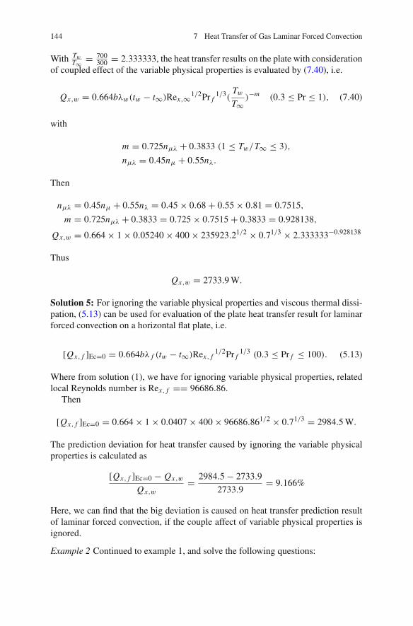
144 7 Heat Transfer of Gas Laminar Forced Convection
With TwT∞ = 700
300 = 2.333333, the heat transfer results on the plate with considerationof coupled effect of the variable physical properties is evaluated by (7.40), i.e.
Qx,w = 0.664bλw(tw − t∞)Rex,∞1/2Pr f1/3(
TwT∞
)−m (0.3 ≤ Pr ≤ 1), (7.40)
with
m = 0.725nμλ + 0.3833 (1 ≤ Tw/T∞ ≤ 3),
nμλ = 0.45nμ + 0.55nλ.
Then
nμλ = 0.45nμ + 0.55nλ = 0.45 × 0.68 + 0.55 × 0.81 = 0.7515,
m = 0.725nμλ + 0.3833 = 0.725 × 0.7515 + 0.3833 = 0.928138,
Qx,w = 0.664 × 1 × 0.05240 × 400 × 235923.21/2 × 0.71/3 × 2.333333−0.928138
Thus
Qx,w = 2733.9 W.
Solution 5: For ignoring the variable physical properties and viscous thermal dissi-pation, (5.13) can be used for evaluation of the plate heat transfer result for laminarforced convection on a horizontal flat plate, i.e.
[Qx, f ]Ec=0 = 0.664bλ f (tw − t∞)Rex, f1/2Pr f
1/3 (0.3 ≤ Pr f ≤ 100). (5.13)
Where from solution (1), we have for ignoring variable physical properties, relatedlocal Reynolds number is Rex, f == 96686.86.
Then
[Qx, f ]Ec=0 = 0.664 × 1 × 0.0407 × 400 × 96686.861/2 × 0.71/3 = 2984.5 W.
The prediction deviation for heat transfer caused by ignoring the variable physicalproperties is calculated as
[Qx, f ]Ec=0 − Qx,w
Qx,w= 2984.5 − 2733.9
2733.9= 9.166%
Here, we can find that the big deviation is caused on heat transfer prediction resultof laminar forced convection, if the couple affect of variable physical properties isignored.
Example 2 Continued to example 1, and solve the following questions:

7.8 Calculation Examples 145
(1) calculate the average skin-friction coefficient with consideration of variablephysical properties;
(2) calculate the average skin-friction coefficient with ignoring variable physicalproperties.
Solution 1: With (7.29) the average skin-friction coefficient with consideration ofvariable physical properties is as follows:
C x,w = 2 × √2νw
ν∞(Rex,∞)−1/2
(dWx (η)
dη
)
η=0.
From example 1, we have Rex,∞ = 235923.2 and TwT∞ = 2.333333.
For tw = 427◦C and t∞ = 27 ◦C, from Fig. 7.6 we have
νw = 68.1 × 10⁻⁶m2/s, ν∞ = 15.895 × 10⁻⁶m2/s.
With TwT∞ = 2.333333, by using interpolation approach, we have the following value
of(
dWx (η)dη
)η=0
from Table 7.3:
(dWx (η)
dη
)
η=0= 0.226426.
Then, for consideration of variable physical properties, the average skin friction is
Cx,w = 2 × √2 × 68.1
15.895× 235923.2−1/2 × 0.226426
= 0.005649.
Solution 2: With (5.2), the average skin friction with ignoring variable physicalproperties is
Cx, f = 1.328Rex, f−1/2.
Then
Cx, f = 1.328 × 96686.86−1/2 = 0.00427.
Then the relative deviation of the average skin-friction with ignoring variable phys-ical properties to that with consideration of variable physical properties is
C x, f − Cx,w
Cx,w= 0.00427 − 0.005649
0.005649= −0.244 = −24.4%.
146 7 Heat Transfer of Gas Laminar Forced Convection
These examples demonstrate that ignoring the variable physical properties willcause very large deviation on prediction of heat transfer and momentum issue.
Exercises
1. According to this chapter, try to explain the importance and necessity for consid-eration of variable physical properties in theoretical investigation on heat transferof gas laminar forced convection.
2. Please try to use Falkner–Skan-type transformation reviewed in Chap. 3, alsotransform similarly the governing partial differential equations (7.1), (7.2), and(7.3) as well as their boundary condition equations (7.4) and (7.5) to the corre-sponding governing ordinary differential equations.
3. On the basis of solution of Example 1, please compare in detail the similaritygoverning ordinary equations with consideration of variable physical propertiesbased on the present new similarity analysis method and Falkner-Skan type trans-formation. What conclusions would you have from such comparison?
4. Follow Example 1, the air is replaced by a typical waste gas of the furnacewhose Prandtl number, viscous parameter, and thermal conductivity parameterare 0.63, 0.75, and 1.02, respectively, and keep all other conditions. Please solvethe following:
(1) evaluate the related local Reynolds numbers for determination of the flowtypes;
(2) calculate the related Eckert numbers;(3) determine the related heat transfer prediction deviation caused by ignoring
the viscous thermal dissipation;(4) calculate the related heat transfer results with consideration of coupled effect
of the variable physical properties;(5) evaluate the prediction deviation on heat transfer caused by ignoring the
variable physical properties.(6) calculate the average skin-friction coefficient with consideration of variable
physical properties;(7) calculate the average skin-friction coefficient with ignoring variable physical
properties.
References
1. H. Blasius, Grenzschichten in Flussigkeiten mit kleiner Reibung, Z. Math. Phys. 56, 1–37(1908)
2. E. Pohlhausen, Der Wärmeaustausch zwischen festen Körpern und Flüssigkeiten mit kleinerReibung und kleiner Wärmeleitung. Z. Angew. Math. Mech. 1, 115–121 (1921)
3. H. Schlichting, J. Kestin, Boundary Layer Theory (McGraw-Hill, New York, NY, 1955)4. J.X. Ling, A. Dybbs, Forced convection over a flat plate submersed in a porous medium: vari-
able viscosity case. Paper 87-WA/HT-23, New York, ASME, (1987)

References 147
5. J.X. Ling, A. Dybbs, The effect of variable viscosity on forced convection. J. Heat Transfer114, 1063 (1992)
6. A. Postelnicu, T. Grosan, I. Pop, The effect of variable viscosity on forced convection flow pasta horizontal flat plate in a porous medium with internal heat generation. Mech. Res. Commun.28(3), 331–337 (2001)
7. D.Y. Shang, Free Convection Film Flows and Heat Transfer (Springer, Berlin, Heidelberg andNew York, NY, 2006)
8. D.Y. Shang, B.X. Wang, Effect of variable thermophysical properties on laminar free convectionof gas. Int. J. Heat Mass Transfer 33(7), 1387–1395 (1990)
9. D.Y. Shang, B. X. Wang, Effect of variable thermophysical properties on laminar free convec-tion of polyatomic gas. Int. J. Heat Mass Transfer 34(3), 749–755 (1991)


Chapter 8Heat Transfer of Liquid Laminar ForcedConvection with Consideration of VariablePhysical Properties
Abstract The new similarity analysis method is applied to develop a novel systemof analysis and transformation models of liquid laminar forced convection withconsideration of variable physical properties. As an example, the formulatedtemperature-dependent equations on density, thermal conductivity, absolute viscos-ity of water, and specific heat are applied, and the reliable numerical solutionson water laminar forced convection are obtained for investigation of the coupledeffect of these variable physical properties. Theoretical equations on heat transferare obtained based on the new similarity model, where the wall dimensionless tem-perature gradient is the no-given variable. The system of key numerical solutionson the wall dimensionless temperature gradient is formulated by a curve-fittingapproach. Combined with the formulated equations of the wall dimensionless tem-perature gradient, the theoretical equations on heat transfer become available forsimple and reliable prediction of heat transfer of water laminar forced convectionwith consideration of coupled effect of the variable physical properties.
8.1 Introduction
In Chap. 7, we investigated heat transfer of gas laminar forced convection with con-sideration of the coupled effect of variable thermophysical properties. In that investi-gation, the temperature-dependent physical properties at atmospheric pressure, suchas density, thermal conductivity, specific heat, and absolute viscosity, are treated by asimple power law with the related temperature parameters. While, for general gases,the specific heat parameter is so small compared with other temperature parameters,their specific heat can be regarded as constant with temperature. Based on the newsimilarity analysis method, in the transformed governing ordinary differential equa-tions the variable physical properties exist in form of the dimensionless physicalproperty factors, which are late treated to the function of the dimensionless temper-ature variable, related temperature parameters, and boundary temperature ratio. Onthis basis, the developed dimensionless governing differential equations are solved
D.Y. Shang, Theory of Heat Transfer with Forced Convection Film Flows,Heat and Mass Transfer, DOI 10.1007/978-3-642-12581-2_8,C© Springer-Verlag Berlin Heidelberg 2011
149
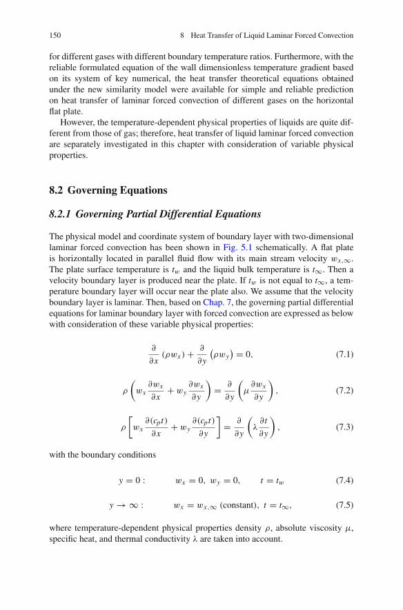
150 8 Heat Transfer of Liquid Laminar Forced Convection
for different gases with different boundary temperature ratios. Furthermore, with thereliable formulated equation of the wall dimensionless temperature gradient basedon its system of key numerical, the heat transfer theoretical equations obtainedunder the new similarity model were available for simple and reliable predictionon heat transfer of laminar forced convection of different gases on the horizontalflat plate.
However, the temperature-dependent physical properties of liquids are quite dif-ferent from those of gas; therefore, heat transfer of liquid laminar forced convectionare separately investigated in this chapter with consideration of variable physicalproperties.
8.2 Governing Equations
8.2.1 Governing Partial Differential Equations
The physical model and coordinate system of boundary layer with two-dimensionallaminar forced convection has been shown in Fig. 5.1 schematically. A flat plateis horizontally located in parallel fluid flow with its main stream velocity wx,∞.The plate surface temperature is tw and the liquid bulk temperature is t∞. Then avelocity boundary layer is produced near the plate. If tw is not equal to t∞, a tem-perature boundary layer will occur near the plate also. We assume that the velocityboundary layer is laminar. Then, based on Chap. 7, the governing partial differentialequations for laminar boundary layer with forced convection are expressed as belowwith consideration of these variable physical properties:
∂
∂x(ρwx )+ ∂
∂y
(ρwy) = 0, (7.1)
ρ
(wx∂wx
∂x+ wy
∂wx
∂y
)= ∂
∂y
(μ∂wx
∂y
), (7.2)
ρ
[wx∂(cpt)
∂x+ wy
∂(cpt)
∂y
]= ∂
∂y
(λ∂t
∂y
), (7.3)
with the boundary conditions
y = 0 : wx = 0, wy = 0, t = tw (7.4)
y → ∞ : wx = wx,∞ (constant), t = t∞, (7.5)
where temperature-dependent physical properties density ρ, absolute viscosity μ,specific heat, and thermal conductivity λ are taken into account.

8.2 Governing Equations 151
8.2.2 Similarity Transformation Variables
According to Chap. 7 for the new similarity analysis method, the set of the relateddimensional analysis variables are shown as follows:
η = y
x
(1
2Rex,∞
)1/2, (7.6)
Rex,∞ = wx,∞x
ν∞, (7.7)
wx = wx,∞Wx (η), (7.8)
wy = wx,∞(
1
2Rex,∞
)−1/2
Wy(η), (7.9)
θ(η) = t − t∞tw − t∞
, (7.10)
where η is dimensionless coordinate variable, Rex,∞ is local Reynolds number,Wx (η) and Wy(η) are dimensionless velocity components in x and y coordinatesrespectively, and θ(η) denotes dimensionless temperature.
8.2.3 Governing Ordinary Differential Equations
Consulting the derivation in Chap. 7, the transformed governing ordinary differen-tial equations for laminar forced convection are
−ηdWx (η)
dη+ 2
dWy(η)
dη+ 1
ρ
dρ
dη[−η · Wx (η)+ 2Wy(η)] = 0, (7.11)
ν∞ν(−ηWx (η)+ 2Wy(η))
dWx (η)
dη= d2Wx (η)
dη2+ 1
μ
dμ
dη
dWx (η)
dη, (7.12)
Prν∞ν
[(−ηWx (η)+ 2Wy(η))
dθ(η)
dη+ (−ηWx (η)+ 2Wy(η)
)
×(θ(η)+ t∞
tw − t∞
)1
cp
dcp
dη
]= d2θ(η)
dη2 + 1
λ
∂λ
∂η
dθ(η)
dη(7.13)
with the boundary condition equations
η = 0 : Wx (η) = 0, Wy(η) = 0, θ(η) = 1 (7.14)
η → ∞ : Wx (η) = 1, θ(η) = 0 (7.15)
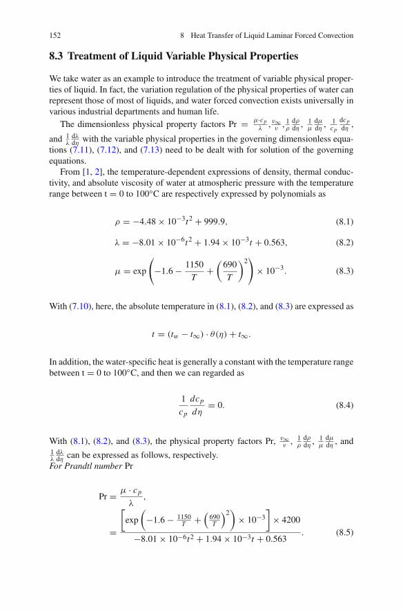
152 8 Heat Transfer of Liquid Laminar Forced Convection
8.3 Treatment of Liquid Variable Physical Properties
We take water as an example to introduce the treatment of variable physical proper-ties of liquid. In fact, the variation regulation of the physical properties of water canrepresent those of most of liquids, and water forced convection exists universally invarious industrial departments and human life.
The dimensionless physical property factors Pr = μ·cpλ
, ν∞ν
, 1ρ
dρdη , 1
μdμdη , 1
cp
dcpdη ,
and 1λ
dλdη with the variable physical properties in the governing dimensionless equa-
tions (7.11), (7.12), and (7.13) need to be dealt with for solution of the governingequations.
From [1, 2], the temperature-dependent expressions of density, thermal conduc-tivity, and absolute viscosity of water at atmospheric pressure with the temperaturerange between t = 0 to 100◦C are respectively expressed by polynomials as
ρ = −4.48 × 10⁻³t2 + 999.9, (8.1)
λ = −8.01 × 10⁻⁶t2 + 1.94 × 10⁻³t + 0.563, (8.2)
μ = exp
(−1.6 − 1150
T+(
690
T
)2)
× 10−3. (8.3)
With (7.10), here, the absolute temperature in (8.1), (8.2), and (8.3) are expressed as
t = (tw − t∞) · θ(η)+ t∞.
In addition, the water-specific heat is generally a constant with the temperature rangebetween t = 0 to 100◦C, and then we can regarded as
1
cp
dcp
dη= 0. (8.4)
With (8.1), (8.2), and (8.3), the physical property factors Pr, ν∞ν
, 1ρ
dρdη , 1
μdμdη , and
1λ
dλdη can be expressed as follows, respectively.
For Prandtl number Pr
Pr = μ · cp
λ,
=
[exp
(−1.6 − 1150
T +(
690T
)2)
× 10−3]
× 4200
−8.01 × 10⁻⁶t2 + 1.94 × 10⁻³t + 0.563. (8.5)

8.3 Treatment of Liquid Variable Physical Properties 153
While the physical property factors 1ρ
dρdη , 1
μdμdη and 1
λdλdη are treated as below:
For physical property factor 1ρ
dρdη
The physical property factor 1ρl
dρdη is expressed as
1
ρ
dρ
dη= 1
ρ
dρ
dt
dt
dη. (a)
With (8.1), the following equation is obtained
dρ
dt= −2 × 4.48 × 10−3t. (b)
With (7.10) we obtain
dt
dη= (tw − t∞)
dθ(η)
dη. (c)
Then
1
ρ
dρ
dη=(−2 × 4.48 × 10−3t)(tw − t∞)
dθ(η)
dη−4.48 × 10⁻³t2 + 999.9
. (8.6)
For physical property factor 1λ
dλdη
The physical property factor 1λ
dλdη is expressed as
1
λ
dλ
dη= 1
λ
dλ
dt
dt
dη. (d)
With (8.2), the following equation is obtained
dλ
dt= −2 × 8.01 × 10−6t + 1.94 × 10⁻³. (e)
Then (d) becomes
1
λ
dλ
dη=(−2 × 8.01 × 10−6t + 1.94 × 10⁻³)(tw − t∞)
dθ(η)
dη−8.01 × 10⁻⁶t2 + 1.94 × 10⁻³t + 0.563
. (8.7)
For physical property facto 1μ
dμdη
The physical property factor 1μ
dμdη is expressed as
1
μ
dμ
dη= 1
μ
dμ
dT
dT
dη. (f)

154 8 Heat Transfer of Liquid Laminar Forced Convection
With (8.3), we have
dμ
dT= exp
[−1.6 − 1150
T+(
690
T
)2]
× 10−3 ·(
1150
T 2 − 2 × 6902
T 3
). (g)
Then, (f) becomes
1
μ
dμ
dη=(
1150
T 2 − 2 × 6902
T 3
)(Tw − T∞)
dθ(η)
dη. (8.8)
For physical property factoν∞ν
ν∞ν
is expressed as
ν∞ν
=(μ∞ρ∞
)/(μ
ρ
)=(μ∞μ
)(ρ
ρ∞
),
=exp
[−1.6 − 1150
T∞ +(
690T∞
)2]
exp
[−1.6 − 1150
T +(
690T
)2] × −4.48 × 10⁻³t2 + 999.9
−4.48 × 10⁻³t2∞ + 999.9, (8.9)
where
t = (tw − t∞) · θ(η)+ t∞ T = t + 273.
Thus, with (8.5), (8.6), (8.7), (8.8), and (8.9), all physical property factors in govern-ing ordinary differential equations (7.11) and (7.13) become function of the dimen-sionless temperature θ(η).
8.4 Velocity and Temperature Fields
Due to the temperature-dependent physical properties, the governing equations(7.11) to (7.13) are coupled with each other, and both velocity and temperature fielddepend on Prandtl number and the temperature boundary conditions. The above cou-pled equations (7.11), (7.12), and (7.13) with the boundary equations (14) and (15)are solved by a shooting method program with fifth-order Runge-Kutta integration.For solving the nonlinear problem, a special variable mesh approach is applied tothe numerical procedure. In this present work, water laminar forced convection ona horizontal flat plate is taken as example for numerical calculation, and a systemof rigorous numerical results of the velocity and temperature fields are obtainedand plotted in Figs. 8.1, 8.2, 8.3, and 8.4, respectively, for the bulk temperatures

8.4 Velocity and Temperature Fields 155
1
11
0
0.2
0.4
0.6
0.8
1
Water forced convectionPr∞ = 9.42t∞=10o C
η η(a)
0 1 2 3 4 65
(b)
0
0.2
0.4
0.6
0.8
1
0 1 2 3 4 65
1
11
Water forced convectionPr∞ = 9.42t∞=10oC
Wx
(η)
θ (η
)
Fig. 8.1 (a) Velocity and (b) temperature profiles of water laminar forced convection on ahorizontal plate with the bulk temperature t∞ = 10◦C and variation of the wall temperature twNote: Lines 1 to 11: for tw = 0, → 10, 20, 30, 40, 50, 60, 70, 80,90 and 100◦C (i.e. tw−t∞ = −10,→ 0, 10, 20, 30, 40, 50, 60, 70, 80, and 90 ◦C)
11
1
111
0
0.2
0.4
0.6
0.8
1
0
0.2
0.4
0.6
0.8
1
(b)
0 1 2 3 4 65
(a)
0 1 2 3 4 65η η
θ (η)
Water forced convectionPr∞ = 4.34t∞ = 40oC
Water forced convectionPr∞ = 4.34t∞ = 40oC
Wx
(η)
Fig. 8.2 (a) Velocity and (b) temperature profiles of water laminar forced convection on ahorizontal plate with the bulk temperature t∞ = 40◦C and variation of the wall temperature twNote: Lines 1 to 11: for tw = 0, 10, 20, 30, → 40, 50,60, 70, 80, 90 and 100 ◦C (i.e. tw−t∞ = −40,−30, −20, −10, → 0, 10, 20, 30, 40, 50, and 60 ◦C)
1
11
1
11
0
0.2
0.4
0.6
0.8
1
0
0.2
0.4
0.6
0.8
1
η η(a)
0 1 2 3 4 65
(b)
0 1 2 3 4 65
θ (η)
Water forced convectionPr∞ = 2.57t∞ = 70oC
Water forced convectionPr∞ = 2.57t∞ = 70oC
Wx
(η)
Fig. 8.3 (a) Velocity and (b) temperature profiles of water laminar forced convection on ahorizontal plate with the bulk temperature t∞ = 70◦C and variation of the wall temperature twNote: Lines 1 to 11: for tw = 0, 10, 20, 30, 40, 50, 60, → 70, 80, 90 and 100◦C (i.e. tw−t∞ = −70,−60, −50, −40, −30, −20, −10, → 0, 10, 20, and 30◦C)

156 8 Heat Transfer of Liquid Laminar Forced Convection
11
1 1
11
0
0.2
0.4
0.6
0.8
1
0
0.2
0.4
0.6
0.8
1
η η(a)
0 1 2 3 4 65
(b)
0 1 2 3 4 65
θ(η)
Water forced convectionPr∞ = 1.76t∞ = 100°C
Water forced convectionPr∞ = 1.76t∞ = 100°C
Wx
(η)
Fig. 8.4 (a) Velocity and (b) temperature profiles of water laminar forced convection on ahorizontal plate with the bulk temperature t∞ =100◦C and variation of the wall temperature twNote: Lines 1 to 11: for tw = 0, 10, 20, 30, 40, 50, 60, 70, 80, 90 and → 100◦C (i.e. tw − t∞ =−100, −90, −80, −70, −60, −50, −40, −30, −20, −10, and → 0◦C)
t∞ = 10◦C, 40◦C, 70◦C), and 100◦C with variations of the wall temperature respec-tively, where the following phenomena are found.
It is seen that, for special bulk temperature t∞ (or special Pr∞), increasing theboundary temperature difference tw − t∞ (i.e. increasing tw or decreasing Prw) willcause increase of dimensionless velocity field level and wall dimensionless temper-ature gradient.
It is obvious that the velocity boundary layer thickness is larger than that oftemperature boundary thickness for liquid laminar forced convection. This phe-nomenon is different from that for gas laminar forced convection, since the Prandtlnumber of liquid is much larger than that of gas. For the same reason, the differencebetween the velocity and temperature boundary layer thicknesses is even obviouswith decreasing t∞ (i.e. increasing Pr∞) for most of laminar forced convection ofliquid, whose Prandtl number increases with decreasing temperature.
All above phenomena demonstrate the effect of variable physical properties onliquid forced convection. These phenomena are different from those expressed byBlasius and Pohlhausen solutions [3, 4] with ignoring the variable physical proper-ties. Obviously, only in the case for tw − t∞ → 0, Blasius and Pohlhausen solutionsare valid.
8.5 Skin-Friction Coefficient with Consideration of VariablePhysical Properties
Following Chap. 7, the equations of local and average skin-friction coefficient withconsideration of variable physical properties for liquid laminar forced convectionare respectively
Cx,w = √2νw
ν∞(Rex,∞)−1/2
(dWx (η)
dη
)
η=0(7.28)

8.6 Heat Transfer Analysis 157
Fig. 8.5 Wall velocity
gradient(
dWx (η)dη
)η=0
of
water laminar forcedconvection on the horizontalplate. Lines 1 → 8 denotest∞ = 0, 10 20, 30, 40, 60, 80,and 100◦C respectively
0
0.5
1
1.5
2
1
8
) η =
0(
dηdW
x (η
)0 20 40 60 80 100
tw, °C
and
C x,w = 2 × √2νw
ν∞(Rex,∞)−1/2
(dWx (η)
dη
)
η=0. (7.29)
It is seen from (7.28) and (7.29) that the wall dimensionless velocity gradient(dWx (η)
dη
)η=0
is the only one no-given variable for evaluation of the skin-friction
coefficient with consideration of variable physical properties. The numerical solu-
tions on the wall dimensionless velocity gradient(
dWx (η)dη
)η=0
of water laminar
forced convection on a flat plate are plotted in Fig. 8.5, and some of the typicalvalued are listed in Table 7.3 for temperature boundary conditions. It is seen that(
dWx (η)dη
)η=0
depends on bulk Prandtl number Pr∞, and boundary temperatures tw
and t∞. Increasing the temperature tw will cause increasing the wall dimensionless
velocity gradient(
dWx (η)dη
)η=0
proportionally. Decreasing the temperature t∞ will
cause increasing the wall dimensionless velocity gradient(
dWx (η)dη
)η=0
at accelera-
tive pace.
8.6 Heat Transfer Analysis
So far, there has been a lack of theoretical investigation on heat transfer for liquidlaminar forced convection with consideration of coupled effect of variable physicalproperties. This issue will be addressed here in this chapter.
First, it is necessary to review the heat transfer theoretical equations as belowfor laminar forced convection developed in Chap. 7 based on the present similarityanalysis method.
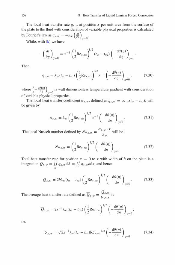
158 8 Heat Transfer of Liquid Laminar Forced Convection
The local heat transfer rate qx,w at position x per unit area from the surface ofthe plate to the fluid with consideration of variable physical properties is calculated
by Fourier’s law as qx,w = −λw(∂t∂y
)y=0
.
While, with (k) we have
−(∂t
∂y
)
y=0= x−1
(1
2Rex,∞
)1/2(tw − t∞)
(−dθ(η)
dη
)
η=0.
Then
qx,w = λw(tw − t∞)(
1
2Rex,∞
)1/2x−1(
−dθ(η)
dη
)
η=0, (7.30)
where(− dθ(η)
dη
)η=0
is wall dimensionless temperature gradient with consideration
of variable physical properties.The local heat transfer coefficient αx,w , defined as qx,w = αx,w(tw − t∞), will
be given by
αx,w = λw
(1
2Rex,∞
)1/2
x−1(
−dθ(η)
dη
)
η=0. (7.31)
The local Nusselt number defined by Nux,w = αx,w · x
λwwill be
Nux,w =(
1
2Rex,∞
)1/2 (−dθ(η)
dη
)
η=0(7.32)
Total heat transfer rate for position x = 0 to x with width of b on the plate is aintegration Qx,w = ∫∫
Aqx,wdA = ∫ x
0 qx,wbdx , and hence
Qx,w = 2bλw(tw − t∞)(
1
2Rex,∞
)1/2 (−dθ(η)
dη
)
η=0. (7.33)
The average heat transfer rate defined as Qx,w = Qx,w
b × xis
Qx,w = 2x−1λw(tw − t∞)(
1
2Rex,∞
)1/2 (−dθ(η)
dη
)
η=0,
i.e.
Qx,w = √2x−1λw(tw − t∞)Rex,∞1/2
(−dθ(η)
dη
)
η=0(7.34)
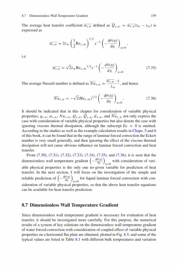
8.7 Dimensionless Wall Temperature Gradient 159
The average heat transfer coefficient αx,w defined as Qx,w = αx,w(tw − t∞) isexpressed as
αx,w = 2λw
(1
2Rex,∞
)1/2
x−1(
−dθ(η)
dη
)
η=0,
i.e.
αx,w = √2λwRex,∞1/2x−1
(−dθ(η)
dη
)
η=0. (7.35)
The average Nusselt number is defined as Nux,w = αx,w · x
λw, and hence
Nux,w = −√2(Rex,∞)1/2
(−dθ(η)
dη
)
η=0. (7.36)
It should be indicated that in this chapter for consideration of variable physicalproperties, qx,w, αx,w, Nux,w, Qx,w, Qx,w, αx,w, and Nux,w not only express thecase with consideration of variable physical properties but also denote the case withignoring viscous thermal dissipation, although the subscript Ec = 0 is omitted.According to the studies as well as the example calculation results in Chaps. 5 and 6of this book, it can be found that in the range of laminar forced convection the Eckertnumber is very small generally, and then ignoring the effect of the viscous thermaldissipation will not cause obvious influence on laminar forced convection and heattransfer.
From (7.30), (7.31), (7.32), (7.33), (7.34), (7.35), and (7.36), it is seen that the
dimensionless wall temperature gradient(− dθ(η)
dη
)η=0
with consideration of vari-
able physical properties is the only one no-given variable for prediction of heattransfer. In the next section, I will focus on the investigation of the simple and
reliable prediction of(− dθ(η)
dη
)η=0
for liquid laminar forced convection with con-
sideration of variable physical properties, so that the above heat transfer equationscan be available for heat transfer prediction.
8.7 Dimensionless Wall Temperature Gradient
Since dimensionless wall temperature gradient is necessary for evaluation of heattransfer, it should be investigated more carefully. For this purpose, the numericalresults of a system of key solutions on the dimensionless wall temperature gradientof water forced convection with consideration of coupled effect of variable physicalproperties on a horizontal flat plate are obtained, plotted in Fig. 8.5, and some of thetypical values are listed in Table 8.1 with different bulk temperatures and variation
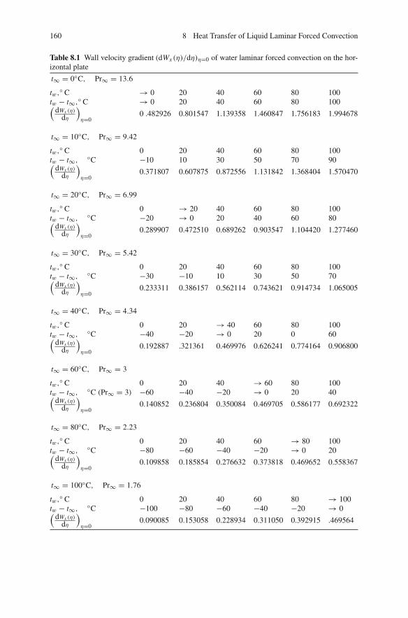
160 8 Heat Transfer of Liquid Laminar Forced Convection
Table 8.1 Wall velocity gradient (dWx (η)/dη)η=0 of water laminar forced convection on the hor-izontal plate
t∞ = 0◦C, Pr∞ = 13.6
tw,◦ C → 0 20 40 60 80 100tw − t∞,◦ C → 0 20 40 60 80 100(
dWx (η)
dη
)η=0
0 .482926 0.801547 1.139358 1.460847 1.756183 1.994678
t∞ = 10◦C, Pr∞ = 9.42
tw,◦ C 0 20 40 60 80 100tw − t∞, ◦C −10 10 30 50 70 90(
dWx (η)
dη
)η=0
0.371807 0.607875 0.872556 1.131842 1.368404 1.570470
t∞ = 20◦C, Pr∞ = 6.99
tw,◦ C 0 → 20 40 60 80 100tw − t∞, ◦C −20 → 0 20 40 60 80(
dWx (η)
dη
)η=0
0.289907 0.472510 0.689262 0.903547 1.104420 1.277460
t∞ = 30◦C, Pr∞ = 5.42
tw,◦ C 0 20 40 60 80 100tw − t∞, ◦C −30 −10 10 30 50 70(
dWx (η)
dη
)η=0
0.233311 0.386157 0.562114 0.743621 0.914734 1.065005
t∞ = 40◦C, Pr∞ = 4.34
tw,◦ C 0 20 → 40 60 80 100tw − t∞, ◦C −40 −20 → 0 20 0 60(
dWx (η)
dη
)η=0
0.192887 .321361 0.469976 0.626241 0.774164 0.906800
t∞ = 60◦C, Pr∞ = 3
tw,◦ C 0 20 40 → 60 80 100tw − t∞, ◦C (Pr∞ = 3) −60 −40 −20 → 0 20 40(
dWx (η)
dη
)η=0
0.140852 0.236804 0.350084 0.469705 0.586177 0.692322
t∞ = 80◦C, Pr∞ = 2.23
tw,◦ C 0 20 40 60 → 80 100tw − t∞, ◦C −80 −60 −40 −20 → 0 20(
dWx (η)
dη
)η=0
0.109858 0.185854 0.276632 0.373818 0.469652 0.558367
t∞ = 100◦C, Pr∞ = 1.76
tw,◦ C 0 20 40 60 80 → 100tw − t∞, ◦C −100 −80 −60 −40 −20 → 0(
dWx (η)
dη
)η=0
0.090085 0.153058 0.228934 0.311050 0.392915 .469564
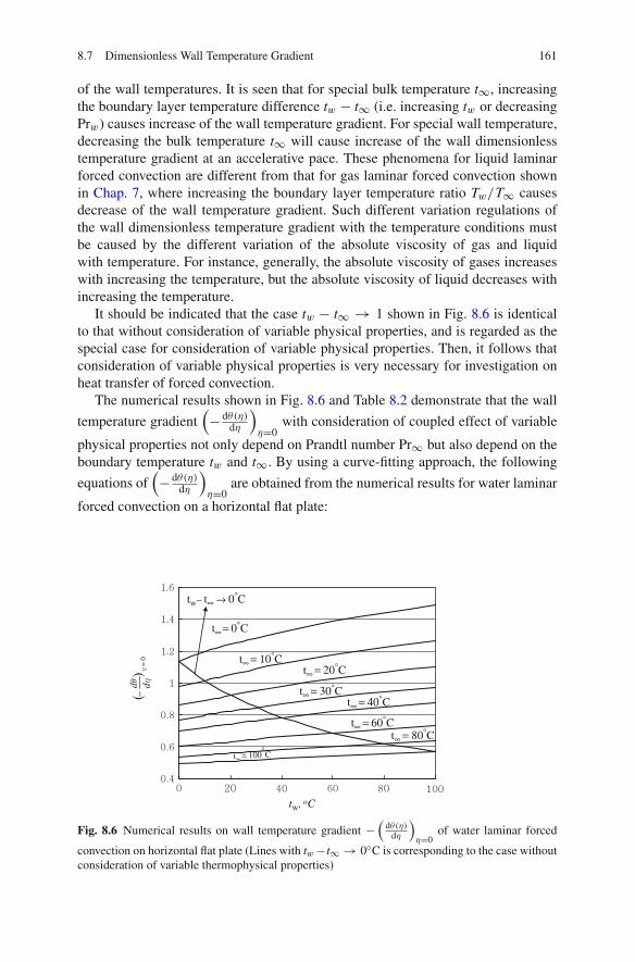
8.7 Dimensionless Wall Temperature Gradient 161
of the wall temperatures. It is seen that for special bulk temperature t∞, increasingthe boundary layer temperature difference tw − t∞ (i.e. increasing tw or decreasingPrw) causes increase of the wall temperature gradient. For special wall temperature,decreasing the bulk temperature t∞ will cause increase of the wall dimensionlesstemperature gradient at an accelerative pace. These phenomena for liquid laminarforced convection are different from that for gas laminar forced convection shownin Chap. 7, where increasing the boundary layer temperature ratio Tw/T∞ causesdecrease of the wall temperature gradient. Such different variation regulations ofthe wall dimensionless temperature gradient with the temperature conditions mustbe caused by the different variation of the absolute viscosity of gas and liquidwith temperature. For instance, generally, the absolute viscosity of gases increaseswith increasing the temperature, but the absolute viscosity of liquid decreases withincreasing the temperature.
It should be indicated that the case tw − t∞ → 1 shown in Fig. 8.6 is identicalto that without consideration of variable physical properties, and is regarded as thespecial case for consideration of variable physical properties. Then, it follows thatconsideration of variable physical properties is very necessary for investigation onheat transfer of forced convection.
The numerical results shown in Fig. 8.6 and Table 8.2 demonstrate that the wall
temperature gradient(− dθ(η)
dη
)η=0
with consideration of coupled effect of variable
physical properties not only depend on Prandtl number Pr∞ but also depend on theboundary temperature tw and t∞. By using a curve-fitting approach, the following
equations of(− dθ(η)
dη
)η=0
are obtained from the numerical results for water laminar
forced convection on a horizontal flat plate:
) η =
0( −
dηdθ
t∞ = 0°C
tw– t∞ → 0°C
tw, oC
t∞ = 10°Ct∞ = 20°C
t∞ = 30°Ct∞ = 40°C
t∞ = 60°Ct∞ = 80°C
t∞ = 100°C
Fig. 8.6 Numerical results on wall temperature gradient −(
dθ(η)dη
)η=0
of water laminar forced
convection on horizontal flat plate (Lines with tw− t∞ → 0◦C is corresponding to the case withoutconsideration of variable thermophysical properties)
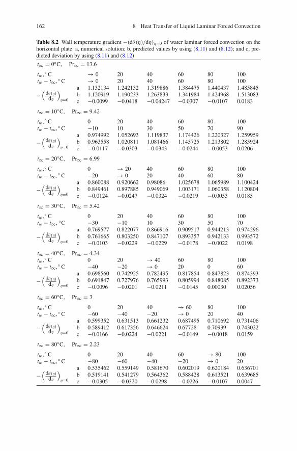
162 8 Heat Transfer of Liquid Laminar Forced Convection
Table 8.2 Wall temperature gradient −(dθ(η)/dη)η=0 of water laminar forced convection on thehorizontal plate. a, numerical solution; b, predicted values by using (8.11) and (8.12); and c, pre-dicted deviation by using (8.11) and (8.12)
t∞ = 0◦C, Pr∞ = 13.6
tw,◦ C → 0 20 40 60 80 100tw − t∞,◦ C → 0 20 40 60 80 100
−(
dθ(η)dη
)η=0
a 1.132134 1.242132 1.319886 1.384475 1.440437 1.485845b 1.120919 1.190233 1.263833 1.341984 1.424968 1.513083c −0.0099 −0.0418 −0.04247 −0.0307 −0.0107 0.0183
t∞ = 10◦C, Pr∞ = 9.42
tw,◦ C 0 20 40 60 80 100tw − t∞,◦ C −10 10 30 50 70 90
−(
dθ(η)dη
)η=0
a 0.974992 1.052693 1.119837 1.174426 1.220327 1.259959b 0.963558 1.020811 1.081466 1.145725 1.213802 1.285924c −0.0117 −0.0303 −0.0343 −0.0244 −0.0053 0.0206
t∞ = 20◦C, Pr∞ = 6.99
tw,◦ C 0 → 20 40 60 80 100tw − t∞,◦ C −20 → 0 20 40 60 80
−(
dθ(η)dη
)η=0
a 0.860088 0.920662 0.98086 1.025678 1.065989 1.100424b 0.849461 0.897885 0.949069 1.003171 1.060358 1.120804c −0.0124 −0.0247 −0.0324 −0.0219 −0.0053 0.0185
t∞ = 30◦C, Pr∞ = 5.42
tw,◦ C 0 20 40 60 80 100tw − t∞, ◦C −30 −10 10 30 50 70
−(
dθ(η)dη
)η=0
a 0.769577 0.822077 0.866916 0.909517 0.944213 0.974296b 0.761665 0.803250 0.847107 0.893357 0.942133 0.993572c −0.0103 −0.0229 −0.0229 −0.0178 −0.0022 0.0198
t∞ = 40◦C, Pr∞ = 4.34tw,◦ C 0 20 → 40 60 80 100tw − t∞,◦ C −40 −20 → 0 20 0 60
−(
dθ(η)dη
)η=0
a 0.698560 0.742925 0.782495 0.817854 0.847823 0.874393b 0.691847 0.727976 0.765993 0.805994 0.848085 0.892373c −0.0096 −0.0201 −0.0211 −0.0145 0.00030 0.02056
t∞ = 60◦C, Pr∞ = 3
tw,◦ C 0 20 40 → 60 80 100tw − t∞,◦ C −60 −40 −20 → 0 20 40
−(
dθ(η)dη
)η=0
a 0.599352 0.631513 0.661232 0.687495 0.710692 0.731406b 0.589412 0.617356 0.646624 0.67728 0.70939 0.743022c −0.0166 −0.0224 −0.0221 −0.0149 −0.0018 0.0159
t∞ = 80◦C, Pr∞ = 2.23
tw,◦ C 0 20 40 60 → 80 100tw − t∞,◦ C −80 −60 −40 −20 → 0 20
−(
dθ(η)dη
)η=0
a 0.535462 0.559149 0.581670 0.602019 0.620184 0.636701b 0.519141 0.541279 0.564362 0.588428 0.613521 0.639685c −0.0305 −0.0320 −0.0298 −0.0226 −0.0107 0.0047

8.7 Dimensionless Wall Temperature Gradient 163
Table 8.2 (continued)
t∞ = 100◦C, Pr∞ = 1.76
tw,◦ C 0 20 40 60 80 → 100tw − t∞,◦ C −100 −80 −60 −40 −20 → 0
−(
dθ(η)dη
)η=0
a 0.492895 0.510384 0.527594 0.543529 0.558004 0.571331b 0.470746 0.488588 0.507106 0.526325 0.546273 0.566977c −0.0449 −0.0427 −0.0388 −0.0317 −0.0210 −0.0076
−(
dθ(η)
dη
)
η=0=[(
−dθ(η)
dη
)
η=0
]
(tw−t∞)→0
exp[(−0.114 × t∞ + 30)
× 10−4 × (tw − t∞)], (8.10)
where
[(−dθ(η)
dη
)η=0
]
(tw−t∞)→0as the reference dimensionless temperature gradi-
ent for ignoring variable physical properties is equivalent to Pohlhausen equation[4] with the reference Prandtl number Pr∞, i.e.
[(−dθ(η)
dη
)
η=0
]
(tw−t∞)→0
= 0.4696 Pr∞1/3, (8.11)
where Pr∞ is reference Prandtl number at bulk temperature as reference tempera-ture. Here, it is seen that (8.10) for consideration of variable thermophysical prop-erties is the spread of the Poulhausen equation. Therefore, consideration of variablethermophysical properties is very necessary and important for reliable and practicalinvestigation of heat transfer on liquid forced convection.
With (8.11), (8.10) becomes
(−dθ(η)
dη
)
η=0= 0.4696 Pr∞1/3 × exp[(−0.114 × t∞ + 30)× 10−4 × (tw − t∞)].
(8.12)
A system of the wall dimensionless temperature gradients(− dθ(η)
dη
)η=0
of water
laminar forced convection on a horizontal flat plate is evaluated by using (8.12)with variation of the bulk Prandtl number, as well as the boundary temperatures twand t∞, and listed in Table 8.2 also. Meanwhile, for the reference Prandtl numberPr∞, the following data are recommended with the reference temperature t∞ forwater shown as in Table 8.3.
It is seen that the evaluated values of(− dθ(η)
dη
)η=0
are pretty well coincident to
the related numerical solutions. Then, it follows that (8.12) is valid for simple and
reliable prediction of the wall dimensionless temperature gradients(− dθ(η)
dη
)η=0
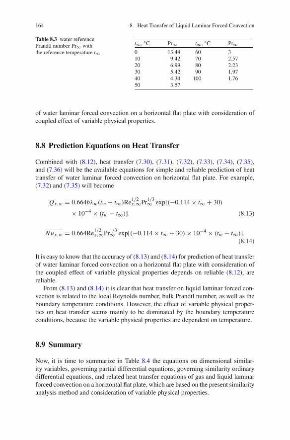
164 8 Heat Transfer of Liquid Laminar Forced Convection
Table 8.3 water referencePrandtl number Pr∞ withthe reference temperature t∞
t∞, ◦C Pr∞ t∞, ◦C Pr∞0 13.44 60 310 9.42 70 2.5720 6.99 80 2.2330 5.42 90 1.9740 4.34 100 1.7650 3.57
of water laminar forced convection on a horizontal flat plate with consideration ofcoupled effect of variable physical properties.
8.8 Prediction Equations on Heat Transfer
Combined with (8.12), heat transfer (7.30), (7.31), (7.32), (7.33), (7.34), (7.35),and (7.36) will be the available equations for simple and reliable prediction of heattransfer of water laminar forced convection on horizontal flat plate. For example,(7.32) and (7.35) will become
Qx,w = 0.664bλw(tw − t∞)Re1/2x,∞Pr1/3∞ exp[(−0.114 × t∞ + 30)
× 10−4 × (tw − t∞)]. (8.13)
Nux,w = 0.664Re1/2x,∞Pr1/3∞ exp[(−0.114 × t∞ + 30)× 10−4 × (tw − t∞)].
(8.14)
It is easy to know that the accuracy of (8.13) and (8.14) for prediction of heat transferof water laminar forced convection on a horizontal flat plate with consideration ofthe coupled effect of variable physical properties depends on reliable (8.12), arereliable.
From (8.13) and (8.14) it is clear that heat transfer on liquid laminar forced con-vection is related to the local Reynolds number, bulk Prandtl number, as well as theboundary temperature conditions. However, the effect of variable physical proper-ties on heat transfer seems mainly to be dominated by the boundary temperatureconditions, because the variable physical properties are dependent on temperature.
8.9 Summary
Now, it is time to summarize in Table 8.4 the equations on dimensional similar-ity variables, governing partial differential equations, governing similarity ordinarydifferential equations, and related heat transfer equations of gas and liquid laminarforced convection on a horizontal flat plate, which are based on the present similarityanalysis method and consideration of variable physical properties.

8.9 Summary 165
Table 8.4 Equations on dimensional similarity variables, governing partial differential equations,governing similarity ordinary differential equations, and related heat transfer equations of gas andliquid laminar forced convection on a horizontal flat plate, which are based on the present similarityanalysis method and consideration of variable physical properties
Governing equations of laminar forced convection on a horizontal flat plate with consideration ofvariable physical propertiesGoverning partial differential equations
Mass equation ∂∂x (ρwx )+ ∂
∂y
(ρwy) = 0
Momentum equation ρ(wx
∂wx∂x + wy
∂wx∂y
)= ∂
∂y
(μ∂wx
∂y
)
Energy equation ρ[wx
∂(cpt)∂x + wy
∂(cpt)∂y
]= ∂
∂y
(λ ∂t∂y
)
Boundary conditions y = 0 : wx = 0, wy = 0, t = twy → ∞ wx = wx,∞ (constant), t = t∞
Equations on dimensionless similarity variables
Local Reynolds number Rex,∞ Rex,∞ = wx,∞xν∞
Coordinate variable η η = yx
(12 Rex,∞
)1/2
Temperature θ θ = t−t∞tw−t∞
Velocity component wx wx = wx,∞ · Wx (η)
Velocity component wy wy = wx,∞(
12 Rex,∞
)−1/2Wy(η)
Governing ordinary differential equations
Mass equation −η dWx (η)
dη + 2 dWy (η)
dη + 1ρ
dρdη [−η · Wx (η)+ 2Wy(η)] = 0
Momentum equation ν∞ν(−ηWx (η)+ 2Wy(η))
∂Wx (η)∂η
= ∂2Wx (η)
∂η2 + 1μ∂μ∂η
∂Wx (η)∂η
Energy equation Pr ν∞ν
[(−ηWx (η)+ 2Wy(η))
dθ(η)dη + (−ηWx (η)
+ 2Wy(η)) (θ(η)+ t∞
tw−t∞
)1
cp
dcp
dη
]
= d2θ(η)
dη2+ 1
λ
∂λ
∂η
dθ(η)
dηBoundary conditions η = 0 : Wx (η) = 0,Wy(η) = 0, θ(η) = 1
η → ∞ : Wx (η) = 1, θ(η) = 0
Physical property factors of the similarity governing mathematical model
Related to gas laminar forcedconvection
1
ρ
dρ
dη= − (Tw/T∞ − 1)dθ(η)/dη
(Tw/T∞ − 1)θ(η)+ 1
1
μ
dμ
dη= nμ(Tw/T∞ − 1)dθ(η)/dη
(Tw/T∞ − 1)θ(η)+ 11
λ
dλ
dη= nλ(Tw/T∞ − 1)dθ(η)/dη
(Tw/T∞ − 1)θ(η)+ 11
cp
dcp
dη= ncp (Tw/T∞ − 1)dθ(η)/dη
(Tw/T∞ − 1)θ(η)+ 1(1
cp
dcp
dηcan be regarded as zero for general gases
)
ν∞ν
= [(Tw/T∞ − 1)θ(η)+ 1]−(nμ+1)
Pr = Pr∞[(Tw/T∞ − 1)θ(η)+ 1]nμ−nλ+ncp
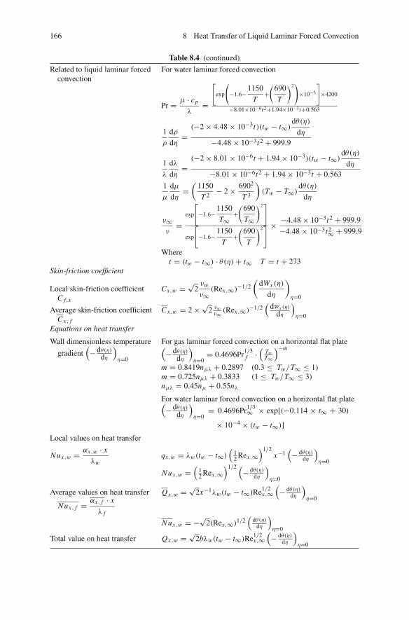
166 8 Heat Transfer of Liquid Laminar Forced Convection
Table 8.4 (continued)
Related to liquid laminar forcedconvection
For water laminar forced convection
Pr = μ · cp
λ=
⎡⎣exp
⎛⎝−1.6− 1150
T+(
690
T
)2⎞⎠×10−3
⎤⎦×4200
−8.01×10⁻⁶t2+1.94×10⁻³t+0.563
1
ρ
dρ
dη=(−2 × 4.48 × 10−3t)(tw − t∞)
dθ(η)
dη−4.48 × 10⁻³t2 + 999.9
1
λ
dλ
dη=(−2 × 8.01 × 10−6t + 1.94 × 10⁻³)(tw − t∞)
dθ(η)
dη−8.01 × 10⁻⁶t2 + 1.94 × 10⁻³t + 0.563
1
μ
dμ
dη=(
1150
T 2− 2 × 6902
T 3
)(Tw − T∞)
dθ(η)
dη
ν∞ν
=exp
⎡⎣−1.6− 1150
T∞+(
690
T∞
)2⎤⎦
exp
⎡⎣−1.6− 1150
T+(
690
T
)2⎤⎦
× −4.48 × 10⁻³t2 + 999.9
−4.48 × 10⁻³t2∞ + 999.9
Wheret = (tw − t∞) · θ(η)+ t∞ T = t + 273
Skin-friction coefficient
Local skin-friction coefficientC f,x
Cx,w = √2νw
ν∞(Rex,∞)−1/2
(dWx (η)
dη
)
η=0
Average skin-friction coefficientCx, f
Cx,w = 2 × √2 νwν∞ (Rex,∞)−1/2
(dWx (η)
dη
)η=0
Equations on heat transfer
Wall dimensionless temperature
gradient(−dθ(η)
dη
)η=0
For gas laminar forced convection on a horizontal flat plate(−dθ(η)
dη
)η=0
= 0.4696Pr1/3f ·(
TwT∞
)−m
m = 0.8419nμλ + 0.2897 (0.3 ≤ Tw/T∞ ≤ 1)m = 0.725nμλ + 0.3833 (1 ≤ Tw/T∞ ≤ 3)nμλ = 0.45nμ + 0.55nλ
For water laminar forced convection on a horizontal flat plate(−dθ(η)
dη
)η=0
= 0.4696Pr1/3∞ × exp[(−0.114 × t∞ + 30)
× 10−4 × (tw − t∞)]Local values on heat transfer
Nux,w = αx,w · x
λwqx,w = λw(tw − t∞)
(12 Rex,∞
)1/2x−1(− dθ(η)
dη
)η=0
Nux,w =(
12 Rex,∞
)1/2 (− dθ(η)dη
)η=0
Average values on heat transfer
Nux, f = αx, f · x
λ f
Qx,w = √2x−1λw(tw − t∞)Re1/2
x,∞(− dθ(η)
dη
)η=0
Nux,w = −√2(Rex,∞)1/2
(dθ(η)
dη
)η=0
Total value on heat transfer Qx,w = √2bλw(tw − t∞)Re1/2
x,∞(− dθ(η)
dη
)η=0

8.10 Remarks 167
8.10 Remarks
Following the study in Chap. 7 on heat transfer of gas laminar forced convectionfor consideration of variable physical properties, in this chapter, heat transfer onliquid laminar forced convection is further investigated with consideration of vari-able physical properties. Meanwhile, water laminar forced convection on a hori-zontal flat plate was taken as an example for the extensive study. By means ofthe formulated equations of temperature dependent density, thermal conductivity,and absolute viscosity, the set of the physical property factors are transformedto the dimensionless temperature based on the new similarity analysis method.Then, the developed completely dimensionless system with the governing ordi-nary differential equations are conveniently coupled with the set of the transformeddimensionless physical property factors, and solved with the temperature boundaryconditions.
The coupled effect of the variable physical properties, such as density, ther-mal conductivity, and viscosity on laminar liquid forced convection is reflected bythe influence of the boundary temperatures, because these physical properties aretemperature-dependent. For special bulk temperature t∞ (i.e. special Pr∞), increas-ing the boundary temperature difference tw − t∞ (i.e. increasing tw or decreasingPrw), causes increasing the velocity field level and the wall temperature gradi-ent. In addition, for special wall temperaturetw (i.e. special Prw), increasing theboundary temperature difference tw − t∞ (i.e. decreasing t∞ or increasing Pr∞)causes increasing the velocity field level and the wall temperature gradient. All thesephenomena demonstrate the coupled effect of variable physical properties on liquidlaminar forced convection.
Generally, increasing the boundary temperature difference tw − t∞ for liquidlaminar forced convection causes increase of the wall temperature gradient, which isdifferent from that for gas laminar forced convection, where increasing the boundarytemperature ratio Tw/T∞ causes decrease of the wall temperature gradient. Suchreason is based on the different variation regulations between the liquid and gasviscosities with temperature.
Only the solution on case tw − t∞ → 0 for liquid laminar forced convectionwith consideration of variable physical properties is identical to Blasius solutionon the velocity field, and Pohlhausen equation on heat transfer. It demonstratesthe limitations for consideration of constant physical properties for investigationof convection heat transfer.
The temperature boundary layer is much narrower than the related velocityboundary layer for liquid laminar forced convection, and increasing the bulk Prandtlnumber Pr∞ causes decreasing the temperature boundary layer thickness.
The system of key solutions on the wall dimensionless temperature gradient forwater laminar free convection on a horizontal flat plate was formulated by using acurve-fitting approach, and the formulated equation is a function of the bulk Prandtlnumber, as well as the boundary temperatures tw and t∞, which demonstrates thecoupled effect of the variable thermophysical properties. The formulated equation

168 8 Heat Transfer of Liquid Laminar Forced Convection
on the wall dimensionless temperature gradient is so reliable that its predicted resultsare pretty well coincident with the related rigorous numerical solutions.
The theoretical equations for heat transfer rate, heat transfer coefficient, and Nes-sult number are reported based on the heat transfer analysis with the new similaritysystem method. In these theoretical equations, the only unknown variable is thewall dimensionless temperature gradient. Combined with the reliable formulatedequations on the wall dimensionless temperature gradient, these analysis equationsare available for simple and reliable prediction on heat transfer of water laminarforced convection. These prediction equations on heat transfer show that heat trans-fer for liquid laminar forced convection with consideration of variable thermophys-ical properties depend on local Reynolds number and local Prandtl number, as wellas the boundary temperature tw and t∞, while heat transfer without consideration ofthermophysical properties is only its special case with tw − t∞ → 0.
Obviously, the analysis presented here extends the previous studies for liquidlaminar forced convection.
8.11 Calculation Examples
Example 1 A flat plate with b = 1 m in width and x = 0.25 m in length is hori-zontally located in water flowing with the velocity wx,∞ = 1.3 m/s. The surfacetemperature of the plate is tw = 70◦C, and water temperature is t∞ = 10◦C. Pleasesolve the following questions:
(1) evaluate the related local Reynolds number for determination the flow types(laminar or turbulent flows);
(2) calculate the related Eckert number;(3) determine the related heat transfer prediction deviation caused by ignoring the
viscous thermal dissipation;(4) calculate the related heat transfer results with consideration of coupled effect of
the variable thermophysical properties;(5) evaluate the heat transfer prediction deviation caused by ignoring the variable
thermophysical properties.
Solution 1: The boundary layer average temperature t f = tw+t∞2 = 70+10
2 = 40◦C.The related physical properties are listed in Table 8.4.
Figure 8.4 Water physical properties
Temperaturetw,◦ C t∞,◦ C. t f ,
◦ C
70 10 40
PhysicalProperties
λw W/(m ◦C)
νw × 10−6
m2/sν∞ × 10−6
m2/sPr∞ Pr f cp kJ/
(kg ◦C)ν f ×10−6
m2/sλ f W/(m ◦C)
0.662 0.4014 1.2996 9.42 4.32 4179 0.6564 0.63

8.11 Calculation Examples 169
Local Reynolds number with ignoring variable physical properties for water isevaluated as
Rex, f = wx,∞x
ν f= 1.3 × 0.25
0.6564 × 10−6= 495124.9< 5×10⁶. Then, it can be regarded
as laminar flow.
Solution 2: The Eckert number is evaluated as
Ec = wx,∞2
cp f (tw − t∞)= 1.32
4179 × 60= 6.74 × 10⁻⁶
With such small Eckert number, the effect of viscous thermal dissipation on heattransfer will be very small, and can be ignored.
Solution 3: With Ec = 6.74 × 10⁻⁶ and Pr f = 4.32, the heat transfer predictiondeviation caused by ignoring the viscous thermal dissipation can be evaluated as
E(Qx, f )Ec=0 = E(Nux, f )Ec=0= −b · Ec2 + c · Ec
0.4696 Pr f1/3
,
with
b = (−0.0007Prf + 0.002)Prf1.75 and c = (−0.2027 Prf − 0.0929)/Prf
0.15.
Then
b = (−0.0007 × 4.32 + 0.002)× 4.321.75 = −0.01326,
c = (−0.2027 × 4.32 − 0.0929)/4.320.15 = −0.77769,
E(Qx, f )Ec=0 = −−0.01326 × (6.74 × 10−6)2 − 0.77769 × 6.74 × 10−6
0.4696 × 4.321/3
= 6.85 × 10⁻⁶.
It is seen that the effect of viscous thermal dissipation on heat transfer is very smallin this case.
Solution 4: The local Reynolds number with consideration of variable physicalproperties will be
Rex,∞ = wx,∞x
ν∞= 1.3 × 0.25
1.2996 × 10−6 = 250076.9.
With (8.13), the heat transfer result of water laminar forced convection on the hor-izontal plate with consideration of coupled effect of the variable thermophysical
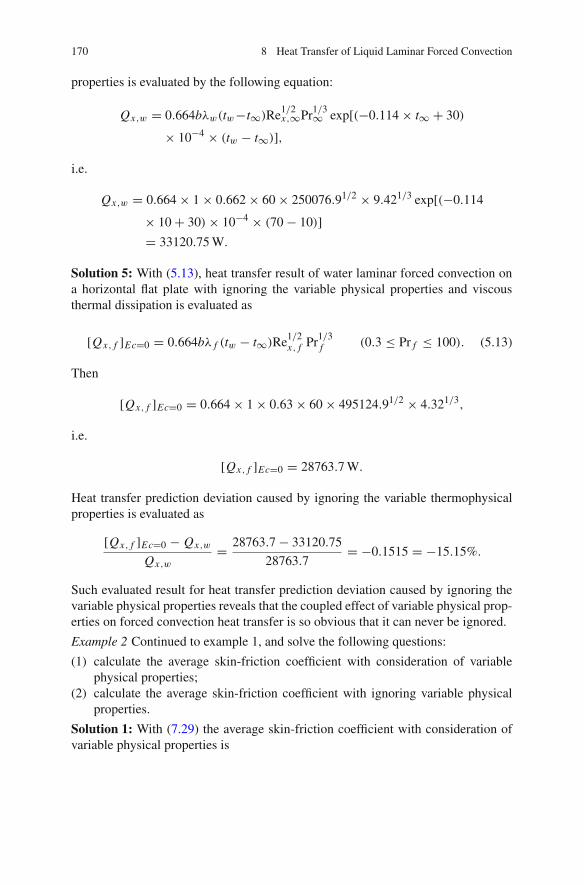
170 8 Heat Transfer of Liquid Laminar Forced Convection
properties is evaluated by the following equation:
Qx,w = 0.664bλw(tw−t∞)Re1/2x,∞Pr1/3∞ exp[(−0.114 × t∞ + 30)
× 10−4 × (tw − t∞)],
i.e.
Qx,w = 0.664 × 1 × 0.662 × 60 × 250076.91/2 × 9.421/3 exp[(−0.114
× 10 + 30)× 10−4 × (70 − 10)]= 33120.75 W.
Solution 5: With (5.13), heat transfer result of water laminar forced convection ona horizontal flat plate with ignoring the variable physical properties and viscousthermal dissipation is evaluated as
[Qx, f ]Ec=0 = 0.664bλ f (tw − t∞)Re1/2x, f Pr1/3
f (0.3 ≤ Pr f ≤ 100). (5.13)
Then
[Qx, f ]Ec=0 = 0.664 × 1 × 0.63 × 60 × 495124.91/2 × 4.321/3,
i.e.
[Qx, f ]Ec=0 = 28763.7 W.
Heat transfer prediction deviation caused by ignoring the variable thermophysicalproperties is evaluated as
[Qx, f ]Ec=0 − Qx,w
Qx,w= 28763.7 − 33120.75
28763.7= −0.1515 = −15.15%.
Such evaluated result for heat transfer prediction deviation caused by ignoring thevariable physical properties reveals that the coupled effect of variable physical prop-erties on forced convection heat transfer is so obvious that it can never be ignored.
Example 2 Continued to example 1, and solve the following questions:
(1) calculate the average skin-friction coefficient with consideration of variablephysical properties;
(2) calculate the average skin-friction coefficient with ignoring variable physicalproperties.
Solution 1: With (7.29) the average skin-friction coefficient with consideration ofvariable physical properties is

8.11 Calculation Examples 171
Cx,w = 2 × √2νw
ν∞(Rex,∞)−1/2
(dWx (η)
dη
)
η=0
From example 1, we have Rex,∞ = 250076.9For tw = 70◦C and t∞ = 10◦C, from Fig. 7.6 we haveνw = 0.4014 × 10⁻⁶, ν∞ = 1.2996 × 10⁻⁶.
With tw = 70◦C and t∞ = 10◦C, by using interpolation approach we have the
following value of(
dWx (η)dη
)η=0
from Table 8.1:
(dWx (η)
dη
)
η=0= 1.25.
Then, for consideration of variable physical properties, the average skin friction is
Cx,w = 2 × √2 × 0.4014
1.2996× 250076.9−1/2 × 1.25
= 0.002184.
Solution 2: From (5.4), we have the equation of the average skin friction with ignor-ing variable physical properties for laminar forced convection on an horizontal flatplate, i.e.
Cx, f = 1.328 Re−1/2x, f . (5.4)
ThenC x, f = 1.328 × 495124.9−1/2 = 0.001887.
Then the relative deviation of the average skin-friction with ignoring variable phys-ical properties to that with consideration of variable physical properties is
Cx, f − Cx,w
Cx, f= 0.001887 − 0.002184
0.001887= −0.1574 = −15.74%
Exercises
1. Can you give an appropriate explanation on the necessity of consideration ofeffect of variable physical properties on liquid laminar forced convection?
2. Based on the general similarity governing mathematical model provided in thischapter, if you are interested in liquid laminar forced convection on a horizontalflat plate with consideration of coupled effect of variable physical properties,you can select any other liquid to investigate reliable heat transfer equations like(8.13) and (8.14) for their reliable application.
172 8 Heat Transfer of Liquid Laminar Forced Convection
3. Based on the analysis approach provided in Chaps. 7 and 8 for derivation of thesimilarity analysis governing mathematical model of laminar forced convectionon a horizontal flat plate, try to investigate the identical similarity analysis gov-erning mathematical model of laminar forced convection with consideration ofvariable physical properties on an inclined flat plate with any inclined angle α.
4. Follow Example 1, the bulk velocity is replaced by 2.6 m/s, the wall temperatureis replaced by 80◦C, but all other conditions are kept. Please solve the following:
(1) evaluate the related local Reynolds number for determination the flow types(laminar or turbulent flows);
(2) calculate the related Eckert number;(3) determine the related heat transfer prediction deviation caused by ignoring
the viscous thermal dissipation;(4) calculate the related heat transfer results with consideration of coupled effect
of the variable physical properties;(5) evaluate the heat transfer prediction deviation caused by ignoring the vari-
able physical properties.(6) calculate the average skin-friction coefficient with consideration of variable
physical properties;(7) calculate the average skin-friction coefficient by ignoring variable physical
properties.
References
1. D.Y. Shang, B.X. Wang, Y. Wang ,Y. Quan, Study on liquid laminar free convection with con-sideration of variable thermophysical properties. Int. J. Heat Mass Transfer 36(14), 3411–3419(1993)
2. D.Y. Shang, Free Convection Film Flows and Heat Transfer (Springer, Berlin, Heidelberg andNew York, NY, 2006)
3. H. Blasius, Grenzschichten in Flussigkeiten mit kleiner Reibung. Z. Math. Phys. 56, 1–37(1908)
4. E. Pohlhausen, Der Wärmeaustausch zwischen festen Körpern und Flüssigkeiten mit kleinerReibung und kleiner Wärmeleitung. Z. Angew. Math. Mech. 1, 115–121 (1921)

Part IIILaminar Forced Film Condensation

Chapter 9Complete Similarity Mathematical Modelson Laminar Forced Film Condensationof Pure Vapour
Abstract The new similarity analysis method is successfully applied in this work,and a complete similarity mathematical model is developed on the laminar forcedfilm condensation of superheated and saturated vapours with consideration of vari-able physical properties. The laminar forced convection film condensation (for short,the laminar forced film condensation, the same below) with two-phase film flowconsists of the condensate liquid film and vapour film, and in both film flows,the variable physical properties are considered. For model of the condensate liquidfilm, the determination of the similarity variables and consideration of the variablephysical properties are based on the approach in Chap. 8 for liquid laminar forcedconvection, while for the model of the vapour film the proposal of the similarityvariables and consideration of the variable physical properties are based on Chap. 7for gas laminar forced convection. The two models are combined with the five inter-facial matching balance equations, respectively describing the velocity componentcontinuity, mass flow rate continuity, the balance of shear force, the energy balance,and the temperature continuity. Based on the new similarity analysis method, thedeveloped system of complete similarity dimensionless model provides conveniencefor treatment of variable physical properties and solution.
9.1 Introduction
Since the pioneer scientist Nusselt published his research [1] on film condensation,numerous studies have followed for laminar free or forced film condensation. Forthe laminar forced film condensation, only some of them, such as in [2–15] are listedhere due to the space limitation. Meanwhile, Cess [2] treated the case where no bodyforce was present and the free stream velocity is very large, and concluded that theresulting interfacial shear stress dominates the heat transfer. Koh [3] developed acomplete numerical solution on the basis of the two-phase boundary-layer equa-tions, using similarity methods. Shekriladze and Gomelauri [4] proposed uniqueapproximate solutions for various cases of condensation, with an assumption that thelocal shearing stress at the interface of vapour and liquid is equal to the momentumgiven up by condensing vapour. Using an approximate integral method, Jakobs [5]obtained good agreement with his experimental results for Freon 113 at atmospheric
D.Y. Shang, Theory of Heat Transfer with Forced Convection Film Flows,Heat and Mass Transfer, DOI 10.1007/978-3-642-12581-2_9,C© Springer-Verlag Berlin Heidelberg 2011
175
176 9 Complete Similarity Mathematical Models
pressure. By using an assuming that vapour outside its boundary is potential flow,Denny and Mills [6] adopted the two-phase boundary layer equations. Beckett andPoots [7] presented the detailed attempt to study laminar film condensation in forcedflows in the context of planar as well as curvilinear geometries. Fujii and Uehara [8]solved two-phase boundary layer equations of laminar film condensation with anapproximate method due to Jacobs. Fujii et al. [9] studied the laminar film conden-sation of flowing vapour on a horizontal cylinder. Rose [10] developed theoreticalequations related to the mass flux of vapour to the condensing surface. Rose [11]
found that when ρvwx,∞2
ρl gd < 18 , the mean heat transfer for the tube is very close
to that found when the pressure gradient is neglected. Honda and Fujii [12] havecarried out conjugate numerical solutions by using a constant inside coolant coef-ficient and solving the two-dimensional conduction problem in the tube wall. Rose[13] provided a new interpolation formula for forced-convection condensation on ahorizontal surface. Memory et al. [14] present the effects of vapour shear, pressuregradient, and surface tension for the laminar condensation on horizontal ellipticaltubes. F. Méndez et al. [15] studied the forced condensation process of a saturatedvapour in contact with one upper surface of a thin plate, taking into account thefinite thermal conductivity of the plate. From them, few studies, such as [3, 6, 8]used the two-phase boundary layer equations to analyze the heat and mass transferof the laminar forced film condensation.
However, in previous studies for dealing with the governing partial differentialequations of the laminar forced convection and film condensation, the traditionalFalkner-Skan type transformation has been universally used. However, with thistransformation method it is difficult to conveniently analyze and treat the variousimportant issues, such as velocity field, interfacial physical balance conditions, con-densate mass transfer, and the variable physical properties for the laminar forcedconvection and film condensation. All these difficult treatments caused a difficultyfor obtaining heat and mass transfer results. Therefore, so far, there still has been alack of a complete similarity model developed to provide the rigorous analysis andnumerical results of the two-phase flow films equations for the rigorous velocity andtemperature distributions, as well as condensate heat mass transfer on the forced filmcondensation.
In this case, the new similarity analysis method reported in Chap. 4 and success-fully applied in Chaps. 5, 6, 7, and 8, respectively, for extensive investigations onlaminar forced convection will be used for resolving these difficult points on thestudy of laminar forced condensation. First, the new similarity analysis method willbe applied for development of the corresponding complete similarity dimensionlessmathematical model. For this purpose, a series of detailed derivations will be donefor similarity transformation under the new similarity analysis system. Meanwhile,with the effective approach on treatment of variable physical properties describedin Chaps. 7 and 8, respectively, for laminar forced convection of gases and liq-uids, the system of the physical properties factor will be similarly transformed tothe function of the dimensionless temperature based on the new similarity analy-sis model. Then, a system of complete governing similarity mathematical modelwill be obtained through a series of rigorously derivation with consideration of

9.2 Governing Partial Differential Equations 177
temperature-dependent physical properties both for liquid and for vapour films. Onthis basis, condensate heat and mass transfer will be deeply investigated based onthe theoretical heat and mass transfer analysis and the system of rigorous numericalsolutions on two-phase film flows velocity and temperature fields.
9.2 Governing Partial Differential Equations
9.2.1 Physical Model and Coordinate System
The present work is focused on the laminar forced film condensation of vapour onan isothermal horizontal flat plate. The analytical model and coordinate system areshown in Fig. 9.1. An isothermal flat plate is located horizontally in a vapour flow atatmospheric pressure. The plate temperature is tw, the temperature and velocity ofthe vapour bulk are t∞ and wx,∞, and the vapour condensate saturated temperatureis ts . If given condition for the model is tw < ts , a steady film condensation willoccur on the plate. We assume that the laminar flows respectively within the liquidand vapour films are induced by the shear force at the liquid–vapour interface. Inaddition, we take into account the temperature-dependent physical properties of thecondensate liquid film and vapour film. Then, the steady laminar governing partialdifferential equations for mass, momentum, and energy in the two-phase boundarylayers are as follows:
Fig. 9.1 Physical model andcoordinate system of thelaminar forced filmcondensation from vapour (δland δv denote liquid andvapour film thicknesses,respectively)
wxv, ∞
x
y
tw
ts
δl δv
wxl wxv
t ∞
tl
tv
9.2.2 Governing Partial Differential Equations
Consulting (7.1), (7.2), and (7.3) for governing partial differential equations of lam-inar forced convection, the governing partial differential equations for condensateliquid and vapour films of laminar forced film condensation of vapour are expressedas follows with consideration of variable physical properties:

178 9 Complete Similarity Mathematical Models
9.2.2.1 For Liquid Film
The governing partial differential equations for condensate liquid film are
∂
∂x(ρlwxl)+ ∂
∂y(ρlwyl) = 0, (9.1)
ρl
(wxl
∂wxl
∂x+ wyl
∂wxl
∂y
)= ∂
∂y
(μl∂wxl
∂y
), (9.2)
ρl
[wxl
∂(cpl t)
∂x+ wyl
∂(cpl t)
∂y
]= ∂
∂y
(λl∂t
∂y
), (9.3)
where (9.1), (9.2), and (9.3) are continuity, momentum, and energy conservationequations, respectively. Here the liquid temperature-dependent physical properties,such as density ρl , absolute viscosity μl , thermal conductivity λl , and specific heatcpl are considered.
9.2.2.2 For Vapour Film
The governing partial differential equations for vapour film are
∂
∂x(ρvwxv)+ ∂
∂y(ρvwyv) = 0, (9.4)
ρv
(wxv
∂wxv
∂x+ wyv
∂wxv
∂y
)= ∂
∂y
(μv∂wxv
∂y
), (9.5)
ρv
(wxv
∂(cpv tv)
∂x+ wyv
∂(cpv tv)
∂y
)= ∂
∂y
(λv∂tv∂y
), (9.6)
where (9.4), (9.5), and (9.6) are continuity, momentum, and energy conservationequations, respectively. Here the vapour temperature-dependent physical properties,such as density ρv , absolute viscosity μv , thermal conductivity λv , and specific heatcpv are considered.
9.2.2.3 For Boundary Conditions
The boundary conditions of the laminar forced film condensation of vapour are
y = 0 : wxl = 0, wyl = 0, tl = tw (9.7)
y = δl : wxl,s = wxv,s (9.8)
ρl,s
(wxl
∂δl
∂x− wyl
)
l,s= ρv,s
(wxv
∂δv
∂x− wyv
)
v,s= gx (9.9)
μl,s
(∂wxl
∂y
)
s= μv,s
(∂wxv
∂y
)
s(9.10)
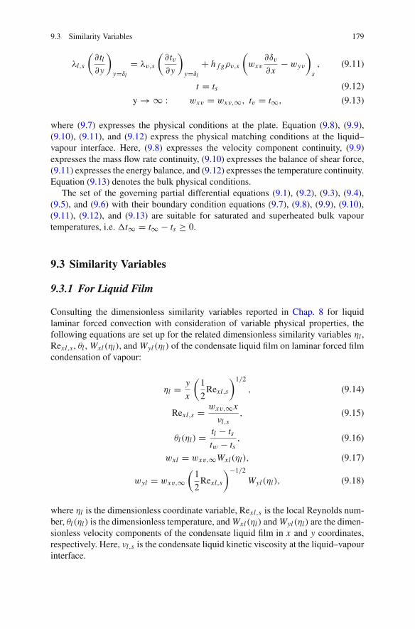
9.3 Similarity Variables 179
λl,s
(∂tl∂y
)
y=δl= λv,s
(∂tv∂y
)
y=δl+ h f gρv,s
(wxv
∂δv
∂x− wyv
)
s, (9.11)
t = ts (9.12)
y → ∞ : wxv = wxv,∞, tv = t∞, (9.13)
where (9.7) expresses the physical conditions at the plate. Equation (9.8), (9.9),(9.10), (9.11), and (9.12) express the physical matching conditions at the liquid–vapour interface. Here, (9.8) expresses the velocity component continuity, (9.9)expresses the mass flow rate continuity, (9.10) expresses the balance of shear force,(9.11) expresses the energy balance, and (9.12) expresses the temperature continuity.Equation (9.13) denotes the bulk physical conditions.
The set of the governing partial differential equations (9.1), (9.2), (9.3), (9.4),(9.5), and (9.6) with their boundary condition equations (9.7), (9.8), (9.9), (9.10),(9.11), (9.12), and (9.13) are suitable for saturated and superheated bulk vapourtemperatures, i.e. �t∞ = t∞ − ts ≥ 0.
9.3 Similarity Variables
9.3.1 For Liquid Film
Consulting the dimensionless similarity variables reported in Chap. 8 for liquidlaminar forced convection with consideration of variable physical properties, thefollowing equations are set up for the related dimensionless similarity variables ηl ,Rexl,s , θl , Wxl (ηl), and Wyl(ηl) of the condensate liquid film on laminar forced filmcondensation of vapour:
ηl = y
x
(1
2Rexl,s
)1/2
, (9.14)
Rexl,s = wxv,∞x
νl,s, (9.15)
θl(ηl) = tl − tstw − ts
, (9.16)
wxl = wxv,∞Wxl(ηl), (9.17)
wyl = wxv,∞(
1
2Rexl,s
)−1/2
Wyl(ηl), (9.18)
where ηl is the dimensionless coordinate variable, Rexl,s is the local Reynolds num-ber, θl(ηl) is the dimensionless temperature, and Wxl(ηl) and Wyl(ηl) are the dimen-sionless velocity components of the condensate liquid film in x and y coordinates,respectively. Here, νl,s is the condensate liquid kinetic viscosity at the liquid–vapourinterface.
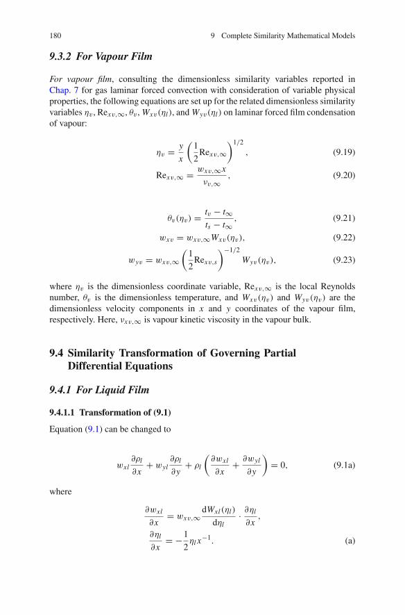
180 9 Complete Similarity Mathematical Models
9.3.2 For Vapour Film
For vapour film, consulting the dimensionless similarity variables reported inChap. 7 for gas laminar forced convection with consideration of variable physicalproperties, the following equations are set up for the related dimensionless similarityvariables ηv , Rexv,∞, θv, Wxv(ηl), and Wyv(ηl) on laminar forced film condensationof vapour:
ηv = y
x
(1
2Rexv,∞
)1/2
, (9.19)
Rexv,∞ = wxv,∞x
νv,∞, (9.20)
θv(ηv) = tv − t∞ts − t∞
, (9.21)
wxv = wxv,∞Wxv(ηv), (9.22)
wyv = wxv,∞(
1
2Rexv,s
)−1/2
Wyv(ηv), (9.23)
where ηv is the dimensionless coordinate variable, Rexv,∞ is the local Reynoldsnumber, θv is the dimensionless temperature, and Wxv(ηv) and Wyv(ηv) are thedimensionless velocity components in x and y coordinates of the vapour film,respectively. Here, νxv,∞ is vapour kinetic viscosity in the vapour bulk.
9.4 Similarity Transformation of Governing PartialDifferential Equations
9.4.1 For Liquid Film
9.4.1.1 Transformation of (9.1)
Equation (9.1) can be changed to
wxl∂ρl
∂x+ wyl
∂ρl
∂y+ ρl
(∂wxl
∂x+ ∂wyl
∂y
)= 0, (9.1a)
where
∂wxl
∂x= wxv,∞
dWxl(ηl)
dηl· ∂ηl
∂x,
∂ηl
∂x= −1
2ηl x
−1. (a)

9.4 Similarity Transformation of Governing Partial Differential Equations 181
With (a) we have
∂wxl
∂x= −1
2ηl x
−1wxv,∞dWxl(ηl)
dηl. (b)
In addition,
wyl = wxv,∞(
1
2Rexl,s
)−1/2
Wyl(ηl),
∂wyl
∂y= wxv,s∞
(1
2Rexl,s
)−1/2 dWyl(ηl)
dηl· ∂ηl
∂y,
∂ηl
∂y= x−1
(1
2Rexl,s
)1/2
. (c)
With (c) we have
∂wyl
∂y= wxv,s∞
dWyl(ηl)
dηl· x−1. (d)
Furthermore,
∂ρl
∂x= dρl
dηl
∂ηl
∂x.
With (a), the above equation becomes
∂ρl
∂x= −1
2
dρl
dηlηl x
−1, (e)
∂ρl
∂y= dρl
dηl
∂ηl
∂y.
With (c) the above equation becomes
∂ρl
∂y= dρl
dηlx−1(
1
2Rexl,s
)1/2
. (f)
With (9.17), (9.18), (b), (d), (e), (f), (9.1a) is changed to
ρl
[−1
2ηl x
−1wxv,∞dWxl(ηl)
dηl+ wxv,s∞
dWyl (ηl)
dηl· x−1]
− 1
2
∂ρl
∂ηlηl x
−1wxv,∞Wxl(ηl )+ dρl
dηlx−1(
1
2Rexl,s
)1/2
wxv,∞(
1
2Rexl,s
)−1/2
Wyl (ηl ) = 0
The above equation is divided by x−1wxv,∞ and becomes
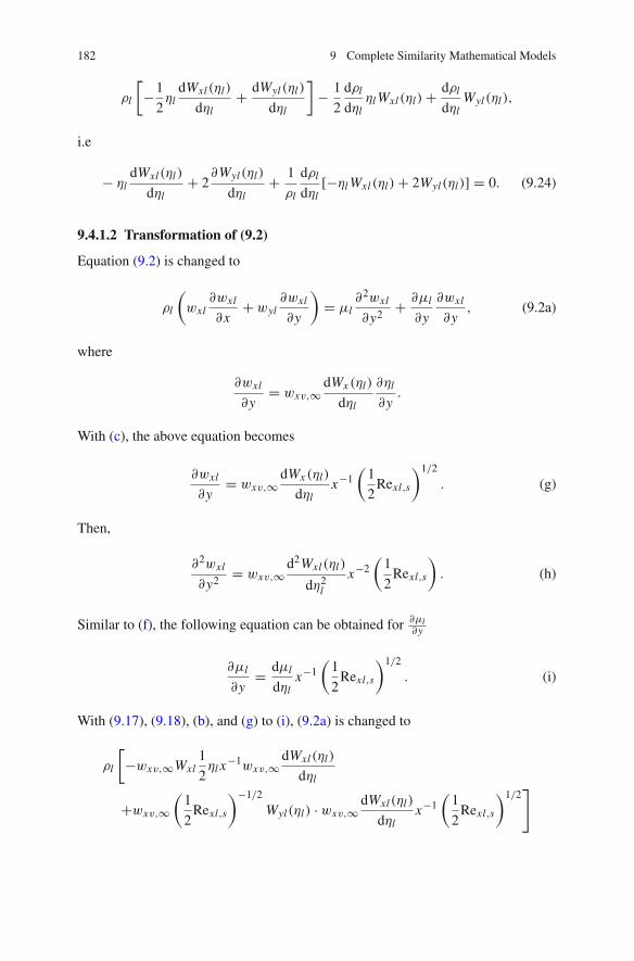
182 9 Complete Similarity Mathematical Models
ρl
[−1
2ηl
dWxl(ηl)
dηl+ dWyl(ηl)
dηl
]− 1
2
dρl
dηlηl Wxl(ηl)+ dρl
dηlWyl(ηl),
i.e
− ηldWxl(ηl)
dηl+ 2
∂Wyl(ηl)
dηl+ 1
ρl
dρl
dηl[−ηl Wxl (ηl)+ 2Wyl(ηl)] = 0. (9.24)
9.4.1.2 Transformation of (9.2)
Equation (9.2) is changed to
ρl
(wxl
∂wxl
∂x+ wyl
∂wxl
∂y
)= μl
∂2wxl
∂y2+ ∂μl
∂y
∂wxl
∂y, (9.2a)
where
∂wxl
∂y= wxv,∞
dWx (ηl)
dηl
∂ηl
∂y.
With (c), the above equation becomes
∂wxl
∂y= wxv,∞
dWx (ηl)
dηlx−1(
1
2Rexl,s
)1/2
. (g)
Then,
∂2wxl
∂y2 = wxv,∞d2Wxl(ηl)
dη2l
x−2(
1
2Rexl,s
). (h)
Similar to (f), the following equation can be obtained for ∂μl∂y
∂μl
∂y= dμl
dηlx−1(
1
2Rexl,s
)1/2
. (i)
With (9.17), (9.18), (b), and (g) to (i), (9.2a) is changed to
ρl
[−wxv,∞Wxl
1
2ηl x
−1wxv,∞dWxl(ηl)
dηl
+wxv,∞(
1
2Rexl,s
)−1/2
Wyl(ηl) · wxv,∞dWxl(ηl)
dηlx−1(
1
2Rexl,s
)1/2]
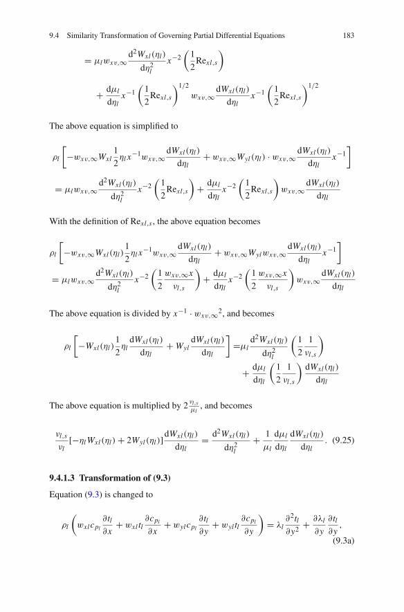
9.4 Similarity Transformation of Governing Partial Differential Equations 183
= μlwxv,∞d2Wxl(ηl)
dη2l
x−2(
1
2Rexl,s
)
+ dμl
dηlx−1(
1
2Rexl,s
)1/2
wxv,∞dWxl(ηl)
dηlx−1(
1
2Rexl,s
)1/2
The above equation is simplified to
ρl
[−wxv,∞Wxl
1
2ηl x
−1wxv,∞dWxl(ηl)
dηl+ wxv,∞Wyl(ηl) · wxv,∞
dWxl(ηl)
dηlx−1]
= μlwxv,∞d2Wxl (ηl)
dη2l
x−2(
1
2Rexl,s
)+ dμl
dηlx−2(
1
2Rexl,s
)wxv,∞
dWxl(ηl)
dηl
With the definition of Rexl,s , the above equation becomes
ρl
[−wxv,∞Wxl(ηl)
1
2ηl x
−1wxv,∞dWxl(ηl)
dηl+ wxv,∞Wylwxv,∞
dWxl(ηl)
dηlx−1]
= μlwxv,∞d2Wxl(ηl)
dη2l
x−2(
1
2
wxv,∞x
νl,s
)+ dμl
dηlx−2(
1
2
wxv,∞x
νl,s
)wxv,∞
dWxl (ηl)
dηl
The above equation is divided by x−1 · wxv,∞2, and becomes
ρl
[−Wxl(ηl)
1
2ηl
dWxl(ηl)
dηl+ Wyl
dWxl (ηl)
dηl
]=μl
d2Wxl(ηl)
dη2l
(1
2
1
νl,s
)
+ dμl
dηl
(1
2
1
νl,s
)dWxl(ηl)
dηl
The above equation is multiplied by 2 νl,sμl
, and becomes
νl,s
νl[−ηl Wxl(ηl)+ 2Wyl(ηl)]dWxl(ηl)
dηl= d2Wxl (ηl)
dη2l
+ 1
μl
dμl
dηl
dWxl(ηl)
dηl. (9.25)
9.4.1.3 Transformation of (9.3)
Equation (9.3) is changed to
ρl
(wxlcpl
∂tl∂x
+ wxl tl∂cpl
∂x+ wylcpl
∂tl∂y
+ wyl tl∂cpl
∂y
)= λl
∂2tl∂y2
+ ∂λl
∂y
∂tl∂y,
(9.3a)
184 9 Complete Similarity Mathematical Models
where
∂tl∂x
= dtldηl
∂ηl
∂x,
while,
∂tl∂ηl
= (tw − ts)dθl(ηl)
dηl. (j)
With (a) and (j), we have
∂tl∂x
= −1
2ηl x
−1(tw − ts)dθl(ηl)
dηl. (k)
Additionally,
∂tl∂y
= dtldηl
∂ηl
∂y.
With (c) and (j), the above equation becomes
∂tl∂y
= x−1(
1
2Rexl,s
)1/2
(tw − ts)dθl(ηl)
dηl. (l)
Then
∂2tl∂y2 = x−2
(1
2Rexl,s
)(tw − ts)
d2tldη2
l
. (m)
Similar to (i), ∂λl∂y and
∂cpl∂y can be expressed as respectively
∂λl
∂y= dλl
dηlx−1(
1
2Rexl,s
)1/2
, (n)
∂cpl
∂y= dcpl
dηlx−1(
1
2Rexl,s
)1/2
. (o)
Similar to (e),∂cpl∂x is expressed as
∂cpl
∂x= −1
2
dcpl
dηlηl x
−1. (p)
With (9.17), (9.18), and (k) to (p), (9.3a) is changed to
9.4 Similarity Transformation of Governing Partial Differential Equations 185
ρl
[wxv,∞Wxl (ηl) cpl
(− 1
2ηl x−1 (tw − ts)dθl (ηl )
dηl
)+ wxv,∞Wxl (ηl ) tl
(− 1
2ηl x−1 dcpldηl
)
+wxv,∞(
12 Rexl,s
)−1/2Wyl (ηl) cpl x−1
(12 Rexl,s
)1/2(tw − ts)
dθl (ηl )dηl
+ wxv,∞(
12 Rexl,s
)−1/2
Wyl (ηl ) tldcpldηl
x−1(
12 Rexl,s
)1/2]
= λl x−2(
12 Rexl,s
)(tw − ts)
d2θl (ηl )
dη2l
+ ∂λl∂ηl
x−1(
12 Rexl,s
)1/2x−1(
12 Rexl,s
)1/2(tw − ts)
dθl (ηl )dηl
With definition of Rexl,s , the above equation is changed to
ρl
⎡⎣wxv,∞Wxl(ηl)cpl
(− 1
2ηl x−1(tw − ts)dθl (ηl )
dηl
)+ wxv,∞Wxl(ηl)tl
(− 1
2ηl x−1 dcpldηl
)
+wxv,∞Wyl(ηl)cpl x−1(tw − ts)
dθl (ηl )dηl
+ wx,∞Wyl (ηl)tldcpldηl
x−1
⎤⎦
= λl x−2(
1
2
wxv,∞x
νl,s
)(tw − ts)
d2θl (ηl)
dη2l
+ dλl
dηlx−1(
1
2
wxv,∞x
νl,s
)x−1(tw − ts)
dθl(ηl)
dηl
The above equation is divided by 12(tw − ts)
cplwxv,∞λl
xνl,s, and simplified to
νl,sρl
λl
⎡⎢⎢⎣
Wxl(ηl)(−ηl
dθl (ηl )dηl
)+ Wxl (ηl)
tltw− ts
(−ηl
1cpl
dcpldηl
)+ 2Wyl(ηl)
dθl (ηl )dηl
+ 2Wyl(ηl)tl
tw− ts1
cpl
dcpldηl
⎤⎥⎥⎦
= 1
cpl
d2θl(ηl)
dη2l
+ 1
cpl
1
λl
dλl
dηl
dθl(ηl)
dηl(9.3b)
With (9.16), we have
tltw − ts
= θl(ηl)+ tstw − ts
. (q)
With (q), (9.3b) is further changed to
cpl νl,sρl
λl
⎡⎣Wxl (ηl )
(−ηl
dθl (ηl )dηl
)+ Wxl (ηl)
[θl(ηl)+ ts
tw− ts
] (−ηl
1cpl
dcpldηl
)
+ 2Wyl (ηl)dθl (ηl )
dηl+ 2Wyl (ηl)
[θl(ηl)+ ts
tw− ts
]1
cpl
dcpldηl
⎤⎦
= d2θl (ηl )
dη2l
+ 1
λl
dλl
dηl
dθl(ηl)
dηl
or
Prlνl,s
νl
⎡⎣−ηl · Wxl(ηl) · dθl (ηl )
dηl+ 2Wyl (ηl ) · dθl (ηl )
dηl− ηl Wxl (ηl)
[θl(ηl )+ ts
tw− ts
] (1
cpl
dcpldηl
)
+ 2Wyl (ηl )[θl (ηl)+ ts
tw− ts
]1
cpl
dcpldηl
⎤⎦
= d2θl (ηl )
dη2l
+ 1
λl
dλl
dηl
dθl(ηl )
dηl

186 9 Complete Similarity Mathematical Models
The above equation is further changed to
Prlνl,s
νl
{[−ηl · Wxl (ηl )+ 2Wyl (ηl)] dθl(ηl)
dηl+ [−ηl Wxl (ηl)+ 2Wyl(ηl)]
[θl(ηl)+ ts
tw − ts
]1
cpl
dcpl
dηl
}
= d2θl (ηl )
dη2l
+ 1
λl
dλl
dηl
dθl(ηl)
dηl(9.26)
9.4.2 For Vapour Film
9.4.2.1 Transformation of (9.4)
Equation (9.4) is changed to
ρv
[∂wxv
∂x+ ∂wyv
∂y
]+ wxv
∂ρv
∂x+ wyv
∂ρv
∂y= 0. (9.4a)
Consulting (a) to (f) for liquid film, we have the following equations for vapour film:
∂ηv
∂x= −1
2ηvx−1, (aa)
∂wxv
∂x= −1
2ηvx−1wxv,∞
dWxv(ηv)
dηv, (bb)
∂ηv
∂y= x−1
(1
2Rexv,∞
)1/2
, (cc)
∂wyv
∂y= wxv,∞
dWyv(ηv)
dηv· x−1, (dd)
∂ρv
∂x= −1
2
dρvdηv
ηvx−1, (ee)
∂ρv
∂y= dρv
dηvx−1(
1
2Rexv,∞
)1/2
. (ff)
With (9.22), (9.23), (bb), (dd), (ee) and (ff), (9.4a) is changed to
ρv
[−1
2ηvx−1wxv,∞
dWxv(ηv)
dηv+ wxv,∞
dWyv(ηv)
dηvx−1]
− 1
2
dρvdηv
ηvx−1wxv,∞Wxv(ηv)+ dρvdηv
x−1[
1
2Rexv,∞
]1/2
wxv,∞(
1
2Rexv,∞
)−1/2
Wyv(ηv) = 0
The above equation is divided by wxv,∞, and simplified to

9.4 Similarity Transformation of Governing Partial Differential Equations 187
ρv
[−1
2ηvx−1 dWxv(ηv)
dηv+ dWyv(ηv)
dηvx−1]
− 1
2
dρvdηv
ηvx−1Wxv(ηv)
+ dρvdηv
x−1Wyv(ηv) = 0.
The above equation is divided by 12 x−1, and simplified to
− ηvdWxv(ηv)
dηv+ 2
dWyv(ηv)
dηv+ 1
ρv
dρvdηv
[−ηvWxv(ηv)+ 2Wyv(ηv)] = 0. (9.27)
9.4.2.2 Transformation of (9.5)
Equation (9.5) is changed to
ρv
(wxv
∂wxv
∂x+ wyv
∂wxv
∂y
)= μv
∂2wxv
∂y2 + ∂μv
∂y
∂wxv
∂y. (9.5a)
Consulting (g) to (h) for liquid film, we have the following equations for vapourfilm:
∂wxv
∂y= wxv,∞
dWxv(ηv)
dηvx−1(
1
2Rexv,∞
)1/2
, (gg)
∂2wxv
∂y2 = wxv,∞d2Wxv(ηv)
dη2v
x−2(
1
2Rexv,∞
), (hh)
∂μv
∂y= dμv
dηvx−1(
1
2Rexv,∞
)1/2
. (ii)
With (9.22), (9.23), (bb), (gg), (hh), and (ii), (9.5a) is changed to
ρv
[−1
2ηvx−1wxv,∞
dWxv (ηv)
dηvwxv,∞Wxv (ηv)+ wxv,∞
(1
2Rexv,s
)−1/2
×Wyv (ηv)wxv,∞dWxv (ηv)
dηvx−1(
1
2Rexv,∞
)1/2]
= μvwxv,∞d2Wxv (ηv)
dη2v
x−2(
1
2Rexv,∞
)+ dμv
dηvx−1(
1
2Rexv,∞
)1/2
wxv,∞dWxv (ηv)
dηvx−1(
1
2Rexv,∞
)1/2
i.e.

188 9 Complete Similarity Mathematical Models
ρv
[−1
2ηvx−1wxv,∞
dWxv (ηv)
dηvwxv,∞Wxv (ηv)+ wxv,∞Wyv (ηv)wxv,∞
dWxv (ηv)
dηvx−1]
= μvwxv,∞d2Wxv (ηv)
dη2v
x−2(
1
2
wxv,∞x
νv,∞
)
+ dμvdηv
x−1(
1
2
wxv,∞x
νv,∞
)wxv,∞
dWxv (ηv)
dηvx−1
The above equation divided by 12w
2xv,∞ · x−1, and becomes
ρv
[−ηvd
dWxv (ηv)
dηvWxv (ηv)+ 2Wyv (ηv)
dWxv(ηv)
dηv
]
= μvd2Wxv (ηv)
dη2v
(1
νv,∞
)+ dμv
dηv
(1
νv,∞
)dWxv (ηv)
dηv
The above equation is divided by μvνv,∞ , and becomes
νv,∞νv
[−ηvWxv(η)+ 2Wyv(η)] dWxv (ηv)
dηv= d2Wxv (ηv)
dη2v
+ 1
μv
dμvdηv
dWxv (ηv)
dηv(9.28)
9.4.2.3 Transformation of (9.6)
Equation (9.6) is changed to
ρv
(wxvcpv
∂tv∂x
+ wxv tv∂cpv
∂x+ wyvcpv
∂tv∂y
+ wyv tv∂cpv
∂y
)= λv
∂2tv∂y2 + ∂λv
∂y
∂tv∂y.
(9.6a)
Consulting (j) to (p) for liquid film, we have the following equations for vapourfilm:
∂tv∂ηv
= (ts − t∞)dθv(ηv)
dηv, (jj)
∂tv∂x
= −1
2ηvx−1(ts − t∞)
dθv(ηv)
dηv, (kk)
∂tv∂y
= x−1(
1
2Rexv,∞
)1/2
(ts − t∞)dθv(ηv)
dηv, (ll)
∂2tv∂y2
= x−2(
1
2Rexv,∞
)(ts − t∞)
d2θv(ηv)
dη2v
, (mm)
9.4 Similarity Transformation of Governing Partial Differential Equations 189
∂λv
∂y= dλv
dηvx−1(
1
2Rexv,∞
)1/2
, (nn)
∂cpv
∂y= dcpv
dηvx−1(
1
2Rexv,∞
)1/2
, (oo)
∂cpv
∂x= −1
2
dcpv
dηvηvx−1. (pp)
With (9.22), (9.23), and (kk) to (pp), (9.6a) is changed to
ρv
⎡⎢⎢⎢⎢⎢⎢⎣
wxv,∞Wxv(ηv)cpv
(−1
2ηvx−1(ts − t∞)
dθv(ηv)
dηv
)+ wxv,∞Wxv(ηv)tv
(−1
2ηvx−1 dcpv
dηv
)
+wxv,∞(
1
2Rexv,∞
)−1/2
Wyv(ηv)cpv x−1(
1
2Rexv,∞
)1/2
(ts − t∞)dθv(ηv)
dηv
+wx,∞(
1
2Rexv,∞
)−1/2
Wyv(ηv)tvdcpvl
dηvx−1(
1
2Rexv,∞
)1/2
⎤⎥⎥⎥⎥⎥⎥⎦
= λl x−2(
1
2Rexv,∞
)(ts − t∞)
d2θv(ηv)
dη2v
+ dλvdηv
x−1(
1
2Rexv,∞
)1/2
x−1(
1
2Rexv,∞
)1/2
(ts − t∞)dθv(ηv)
dηv
i.e.
ρv
⎡⎢⎣
−1
2wxv,∞Wxv(ηv)cpv ηvx−1(ts − t∞)
dθv(ηv)
dηv− 1
2wxv,∞Wxv(ηv)tvηvx−1 dcpv
dηv
+wxv,∞Wyv(ηv)cpv x−1(ts − t∞)dθv(ηv)
dηv+ wx,∞Wyv(ηv)tv
dcpvl
dηvx−1
⎤⎥⎦
= λl x−2(
1
2Rexv,∞
)(ts − t∞)
d2θv(ηv)
dη2v
+ dλvdηv
x−1(
1
2Rexv,∞
)x−1(ts − t∞)
dθv(ηv)
dηv
With definition of Rexv,∞, the above equation is changed to
ρv
⎡⎢⎣
−1
2wxv,∞Wxv(ηv)cpv ηvx−1(ts − t∞)
dθv(ηv)
dηv− 1
2wxv,∞Wxv(ηv)tvηvx−1 dcpv
dηv
+wxv,∞Wyv(ηv)cpv x−1(ts − t∞)dθv(ηv)
dηv)+ wx,∞Wyv(ηv)tv
dcpvl
dηvx−1
⎤⎥⎦
= λvx−2(
1
2
wxv,∞x
νv,∞
)(ts − t∞)
d2θv(ηv)
dη2v
+ dλvdηv
x−1(
1
2
wxv,∞x
νv,∞
)x−1(ts − t∞)
dθv(ηv)
dηv
The above equation is divided by1
2(ts − t∞)
cpvwxv,∞λvxνv,∞
, and simplified to
νv,∞ρvλv
⎡⎢⎢⎣
−Wxv(ηv)ηvdθv(ηv)
dηv− Wxv(ηv)
tvts − t∞
ηv1
cpv
dcpvl
dηv
+ 2Wyv(ηv)dθv(ηv)
dηv)+ 2Wyv(ηv)
tvts − t∞
1
cpv
dcpv
dηv
⎤⎥⎥⎦
= 1
cpv
d2θv(ηv)
dη2v
+ 1
cpv
1
λv
dλvddηv
dθv(ηv)
dηv(9.6b)

190 9 Complete Similarity Mathematical Models
With (9.16), we have
tvts − t∞
= θv(ηv)+ t∞ts − t∞
. (r)
With (q), (9.6b) is further simplified to
Prvνv,∞νv
⎡⎢⎢⎣
−Wxv(ηv)ηvdθv(ηv)
dηv− Wxv(ηv)
(θv(ηv)+ t∞
ts − t∞
)ηv
1
cpv
dcpvl
dηv
+ 2Wyv(ηv)dθv(ηv)
dηv+ 2Wyv(ηv)
(θv(ηv)+ t∞
ts − t∞
)1
cpv
dcpv
dηv
⎤⎥⎥⎦
= d2θv(ηv)
dη2v
+ 1
λv
dλvdηv
dθv(ηv)
dηv
or
Prvνv,∞νv
⎧⎪⎪⎨⎪⎪⎩
[−ηvWxv(ηv)+ 2Wyv(ηv)]dθv(ηv)
dηv
+[−Wxv(ηv)ηv + 2Wyv(ηv)](θv(ηv)+ t∞
ts − t∞
)1
cpv
dcpv
dηv
⎫⎪⎪⎬⎪⎪⎭
= d2θv(ηv)
dη2v
+ 1
λv
dλvdηv
dθv(ηv)
dηv(9.29)
9.4.3 For Boundary Conditions
9.4.3.1 Transformation of (9.7)
With (9.14), (9.16), (9.17) and (9.18), (9.7) can be transformed as easily
ηl = 0 : Wxl (ηl) = 0, Wyl (ηl) = 0, θl (ηl) = 1 (9.30)
9.4.3.2 Transformation of (9.8)
With (9.14) and (9.17), (9.8) is transformed to
ηl = ηlδ(ηv = 0) :Wxv,s(ηv0) = Wxl,s(ηlδ) (9.31)
9.4.3.3 Transformation of (9.9)
With (9.14), (9.15), and (9.17), we have
δl = ηlδ
(1
2
wxv,∞x
νl,s
)−1/2
x,
9.4 Similarity Transformation of Governing Partial Differential Equations 191
∂δl
∂x= 1
2ηlδ
(1
2
wxv,∞x
νl,s
)−1/2
. (s)
Similarly, with (9.19), (9.20), and (9.22), we have
∂δv
∂x= 1
2ηvδ
(1
2
wxv,∞x
νv,∞
)−1/2
. (t)
With ((9.14), (9.17), (9.22), (9.23), (s) and (t), (9.9) is changed to
ρl,s
(wxl
∂δl
∂x− wyl
)
l,s
= ρl,s
[wxv,∞Wxl,s(ηlδ)
1
2ηlδ
(1
2
wxv,∞x
νl,s
)−1/2
− wxv,∞(
1
2
wxv,∞x
νl,s
)−1/2
Wyl,s(ηlδ)
],
ρv,s
(wxv
∂δv
∂x− wyv
)
v,s
= ρv,s
[wxv,∞Wxv,s(ηv0)
1
2ηv0
(1
2
wxv,∞x
νv,∞
)−1/2
− wxv,∞(
1
2
wxv,∞x
νv,∞
)−1/2
Wyv,s (ηv0)
]
v,s
.
Then
ρl,s
[wxv,∞Wxl,s(ηlδ)
1
2ηlδ
(1
2
wxv,∞x
νl,s
)−1/2
− wxv,∞(
1
2
wxv,∞x
νl,s
)−1/2
Wyl,s(ηlδ)
]
= ρv,s
[wxv,∞Wxv,s(ηv0)
1
2ηv0
(1
2
wxv,∞x
νv,∞
)−1/2
− wxv,∞(
1
2
wxv,∞x
νv,∞
)−1/2
Wyv,s(ηv0)
]
Since ηv0 = 0, the above equation becomes
ρl,s
[wxv,∞Wxl,s(ηlδ)
1
2ηlδ
(1
2
wxv,∞x
νl,s
)−1/2
− wxv,∞(
1
2
wxv,∞x
νl,s
)−1/2
Wyl,s(ηlδ)
]
= ρv,s
[−wxv,∞
(1
2
wxv,∞x
νv,∞
)−1/2
Wyv,s(ηv0)
]
Then
Wyv,s(ηv0) =
−ρl,s
[wxv,∞Wxl,s(ηlδ)
1
2ηlδ
(1
2
wxv,∞x
νl,s
)−1/2
− wxv,∞(
1
2
wxv,∞x
νl,s
)−1/2
Wyl,s(ηlδ)
]
ρv,swxv,∞(
1
2
wxv,∞x
νv,∞
)−1/2
The above equation is simplified to
192 9 Complete Similarity Mathematical Models
Wyv,s(ηv0) = −(νl,sνv,∞
)1/2ρl,s
[Wxl,s(ηlδ)
12ηlδ − Wyl,s(ηlδ)
]
ρv,s,
i.e.
Wyv,s(ηv0) = − ρl,s
ρv,s
(νl,s
νv,∞
)1/2 [1
2ηlδ · Wxl,s(ηlδ)− Wyl,s(ηlδ)
](9.32)
9.4.3.4 Transformation of (9.10)
With (g) and (gg), (9.10) is changed to
μl,s
[wxv,∞
dWx (ηl )
dηlx−1(
1
2Rexl,s
)1/2]
s
= μv,s
[wxv,∞
dWxv(ηv)
dηvx−1(
1
2Rexv,∞
)1/2]
s
,
i.e.
μl,swxv,∞(
dWx (ηl)
dηl
)
sx−1(
1
2
wxv,∞x
νl,s
)1/2
= μv,swxv,∞(
dWxv(ηv)
dηv
)
sx−1(
1
2
wx,∞x
νv,∞
)1/2
.
Then
(dWxv(ηv)
dηv
)
s= μl,s
μv,s
(νv,∞νl,s
)1/2 (dWx (ηl)
dηl
)
s. (9.33)
9.4.3.5 Transformation of (9.11)
With (9.22), (9.23), (l), (ll) and (s), (9.11) is changed to
λl,s x−1
[(1
2
wxv,∞x
νl,s
)1/2
(tw − ts)dθl (ηl )
dηl
]
s
=λv,s[
x−1(
1
2
wxv,∞x
νv,∞
)1/2
(ts − t∞)dθv(ηv)
dηv
]
s
+ h f gρv,s
[wxv,∞Wxv(ηv)
1
2ηv0
(1
2
wxv,∞x
νv,∞
)−1/2
− wxv,∞(
1
2
wxv,∞x
νv,∞
)−1/2
Wyv(ηv)
]
s
With ηv0 = 0, the above equation becomes
λl,s x−1
[(1
2
wxv,∞x
νl,s
)1/2
(tw − ts)dθl (ηl)
dηl
]
s
= λv,s
[x−1(
1
2
wxv,∞x
νv,∞
)1/2
(ts − t∞)dθv(ηv)
dηv
]
s
+ h f gρv,s
[−wxv,∞
(1
2
wxv,∞x
νv,∞
)−1/2
Wyv(ηv0)
]
s
9.5 Remarks 193
The above equation is divided by
(1
2wxv,∞
)1/2
·(
1
νv,∞
)1/2
· x−1/2, and simpli-
fied to
λl,s
[(νv,∞νl,s
)1/2
(tw − ts)dθl(ηl )
dηl
]
s
= λv,s
[(ts − t∞)
dθv(ηv)
dηv
]
s+ 2h f gρv,s [−νv,∞Wyv(ηv0)],
i.e.
λv,s
[(ts − t∞)
dθv(ηv)
dηv
]
s= λl,s
[(νv,∞νl,s
)1/2
(tw − ts)dθl(ηl )
dηl
]
s
− 2h f gρv,s [−νv,∞Wyv(ηv0)].
Then
(dθv(ηv)
dηv
)
s=λl,s
(νv,∞νl,s
)1/2
(tw − ts)
(dθl(ηl)
dηl
)
s+ 2h f gρv,sνv,∞Wyv,s(ηv0)
λv,s(ts − t∞).
(9.34)
9.4.3.6 Transformation of (9.12)
With (9.16) and (9.21), (9.12) is changed to
θl(ηlδ) = 0 and θv(ηv0) = 1 (9.35)
9.4.3.7 Transformation of (9.13)
With (9.21) and (9.22), (9.13) becomes
ηv → ∞ Wxv(ηv,∞) = 1, θv(ηv,∞) = 0 (9.36)
9.5 Remarks
With the new similarity analysis method, the complete dimensionless mathemati-cal model is developed for laminar forced film condensation of vapour. The com-plete similarity model consists of liquid and vapour film models, connected by fiveinterfacial matching conditions, respectively, for velocity continuity, mass transferbalance, shear force balance, energy balance, and temperature continuity. Mean-while, both in liquid and vapour films, as well as the interfacial boundary conditionequations, the variable physical properties such as temperature-dependent density,thermal conductivity, viscosity, and specific heat exist in the form of the relateddimensionless physical property factors based on the new similarity analysis system.
The present developed similarity mathematical model is not only suitable forthe laminar forced film condensation of superheated vapour with the superheated
194 9 Complete Similarity Mathematical Models
temperature t∞ − ts > 0 but also suitable for that of saturated vapour with thesuperheated temperature t∞ − ts = 0. In this case, the condensation of saturatedvapour is only regarded as a special case of the superheated vapour.
It is also seen that the new similarity analysis method reported in this book is abetter alternative to the traditional Falkner-Skan type transformation for extensiveinvestigation of laminar film condensation with consideration various physical ele-ments including the complicated interfacial matching conditions and variable phys-ical properties.
Exercises
1. If you like, according to Chap. 3 for reviewing the Falkner–Skan-type trans-formation method, try to transform the governing partial differential equationsand their boundary conditions (9.1)– (9.13) into the related similarity governingmathematical model with consideration of variable physical properties.
2. Compare the similarity governing mathematical model obtained in this chapterfor laminar forced film condensation of vapour with consideration of variablephysical properties based on the present new similarity analysis method withthat based on the Falkner–Skan-type transformation method. Which conclusionscan you get?
3. If the flat plate and the bulk vapour flow have an angle to the horizontal level forlaminar forced film condensation of vapour, please do the following:
(1) Based on (9.1), (9.2), (9.3), (9.4), (9.5), (9.6), (9.7), (9.8), (9.9), (9.10),(9.11), (9.12), and (9.13) for horizontal laminar film condensation of vapour,provide the related governing partial differential equations for the inclinedlaminar film condensation of vapour.
(2) Based on the present new similarity analysis method, provide a new set of theappropriate similarity variables for similarity transformation of the govern-ing partial differential equations for the inclined laminar film condensationof vapour.
(3) By using the new set of the appropriate similarity variables, transform simi-larly the governing partial differential equations together with the boundaryconditions of the inclined laminar film condensation into the related similar-ity governing mathematical model.
(4) Which conclusions do you find from the above work?
References
1. W. Nusselt (1916) Die Oberflächenkondensation des Wasserdampfes. Z. Ver. Dt. Ing.60:541–546, 569–575
2. R.D. Cess, Laminar film condensation on a flat plate in the absence of a body force, Z. Angew.Math. Pfus. 11, 426–433 (1960)
References 195
3. J.C.Y. Koh, Film condensation in a forced-convection boundary-layer flow. Int J Heat MassTransfer 5, 941–954 (1962)
4. I.G. Shekriladze, V.I. Gomelauri, Theoretical study of laminar film condensation of flowingvapor. Int. J. Heat Mass Transfer 9, 581–591 (1966)
5. H.R. Jacobs, An integral treatment of combined body force and forced convection in laminarfilm condensation. Int. J. Heat Mass Transfer 9 637–648 (1966)
6. V.E. Denny, A.F. Mills, Laminar film condensation of a flowingvapor on a horizontal cylinderat normal gravity. ASME J. Heat Transfer 91, 495–501 (1969)
7. P. Beckett, G. Poots, Laminar film condensation in forced flows. Quart. J. Mech. Appl. Maths25(1), 125–152 (1972)
8. T. Fujii, H. Uehara, Laminar filmwise condensation on a vertical surface. Int.I. Heat MassTransfer 15, 217–233 (1972)
9. T. Fujii, H. Honda, K. Oda, Condensation of Steam on a Horizontal Tube—The Influence ofOncoming Velocity and Thermal Condition at the Tube Wall, Condensation Heat Transfer,18th National Heat Transfer Conference. San Diego, CA, 1979, pp. 35–43
10. J.W. Rose, Approximate equation for forced-convection condensation in the presence of a non-condensation gas on a flat plate and horizontal tube. Int. J. Heat Mass Transfer 23, 539–546,(1980)
11. J.W. Rose, Effect of pressurevariation in forced convection film condensation on a horizontaltube. Int. J. Heat Mass Transfer 27(1), 39–47 (1984)
12. H. Honda, T. Fujii, Condensation of a flowing vapor on a horizontal tube – numerical analysison a conjugate heat transfer problem. Trans. ASME. J Heat Transfer 106, 841–848, (1984)
13. J.W. Rose, A new interpolation formula for forced-convection condensation on a horizontalsurface. Trans ASME. J Heat Transfer 111, 818–819 (1989)
14. S.B. Memory, V.H. Adams, Marto, P.J., Free and forced convection laminar film condensationon horizontal elliptical tubes. Int. J. Heat Mass Transfer. 40(14), 3395–3406 (1997)
15. F. Méndez, C. Treviño, Analysis of a forced laminar film condensation including finite longi-tudinal heat conduction effects. Heat Mass Transfer 39, 489–498 (2003)


Chapter 10Velocity and Temperature Fields on LaminarForced Film Condensation of Pure Vapour
Abstract The laminar forced film condensation of water vapour is taken as anexample for treatment of variable physical properties. The temperature parametermethod with the simple power-law equations for gases is used for the treatmentof vapour film variable physical properties, and the water polynomial formulationsare applied for the treatment of liquid film variable physical properties. Then, aneffective numerical procedure is developed for rigorously satisfying a set of theinterfacial physical matching conditions. On this basis, a system of the numericalsolutions on the velocity and temperature fields of the two-phase film flows is rig-orously found out. These numerical solutions demonstrate that increasing the wallsubcooled grade causes increase of the condensate liquid film thickness but decreaseof vapour film thickness, decrease of the wall temperature gradient but increase ofthe vapour film temperature gradient, and increase of the interfacial velocity level.Compared with the effect of the wall subcooled grade on these physical variables,the effect of the vapour subcooled grade is very slight.
10.1 Introduction
In Chap. 9, we obtained the complete dimensionless similarity mathematical modelfor laminar forced film condensation of vapour. Such similarity mathematical modelconsists of two parts of film flows, the liquid film flow and vapour film flow. The twoparts of model are combined by the set of the interfacial matching conditions, i.e.velocity continuity, mass transfer balance, shear force balance, energy balance, andtemperature continuity. In the similarity mathematical model on the laminar forcedfilm condensation, the variable thermophysical properties of gas and liquid exist inthe form of the related dimensionless physical property factors.
The present work is the successive investigation of Chap. 9, and will take thelaminar forced film condensation of water vapour as an example to find out thevelocity and temperature fields of the two-phase film flows. First, the treatment ofthe variable physical properties will be done for liquid and vapour film flows as wellas the interfacial matching condition equations. The temperature parameter methodwith the simple-power law equations reported in [1] and [2], and collected in book[3] is used for the treatment of variable physical properties for vapour film flow,
D.Y. Shang, Theory of Heat Transfer with Forced Convection Film Flows,Heat and Mass Transfer, DOI 10.1007/978-3-642-12581-2_10,C© Springer-Verlag Berlin Heidelberg 2011
197

198 10 Velocity and Temperature Fields
and the polynomial approach [4] are used for treatment of the variable physicalproperties of condensate liquid film low. Then, the set of physical property factorsin the governing similarity mathematical model become the functions of the dimen-sionless temperature based on the new similarity analysis method. On these bases,the developed complete similarity mathematical model on the laminar forced filmcondensation of vapour is solved numerically, in which the set of the interfacialmatching conditions are rigorously satisfied and the variable physical properties ofliquid and vapour films are rigorously treated. Then, a system of solutions with thevelocity and temperature fields is given for different wall subcooled and vapoursuperheated grads, which is a basis on extensive investigation of heat and masstransfer of laminar forced film condensation of vapour.
10.2 Treatment of Temperature-Dependent Physical Properties
As presented in our previous studies such as in [1–6] and Chaps. 7 and 8 of thisbook, it is clear that fluid variable physical properties have great effects on heattransfer with convection and film flows, and so should be appropriately treated forreliable and rigorous solutions of the related governing equations. In this presentwork on the two-phase flow condensation problem, the variable physical propertiesexist respectively in liquid and vapour films and, therefore, should be treated sep-arately. Take the laminar forced film condensation of water vapour as an example,the treatment approach related to the variable physical properties are presented asfollows respectively.
10.2.1 For Liquid Film Medium
Consulting Chap. 8 for treatment approach of liquid variable physical properties, asan example, the water variable density, thermal conductivity, absolute viscosity, andspecific heat are expressed as follows for condensate water film flow:
ρl = −4.48 × 10⁻³t2 + 999.9, (10.1)
λl = −8.01 × 10⁻⁶t2 + 1.94 × 10⁻³t + 0.563, (10.2)
μl = exp
(−1.6 − 1150
T+(
690
T
)2)
× 10−3. (10.3)
While, the water specific heat can be taken as a constant cpl = 4200 J/(kg K) withtemperature variation at atmospheric pressure, and then, specific heat factor can beregarded as

10.2 Treatment of Temperature-Dependent Physical Properties 199
1
cpl
dcpl
dηl= 0. (10.4)
The physical property factors in the governing ordinary differential equations areexpressed as respectively
Prl = μl · cpl
λl=
[exp
(−1.6 − 1150
T+(
690
T
)2)
× 10−3
]× 4200
−8.01 × 10⁻⁶t2 + 1.94 × 10⁻³t + 0.563, (10.5)
1
ρl
dρl
dηl=
[(−2 × 4.48 × 10−3t (tw − ts)
dθl(ηl)
dηl
]
(−4.48 × 10⁻³t2 + 999.9), (10.6)
1
λl
dλl
dηl=
[(−2 × 8.01 × 10−6 + 1.94 × 10⁻³)(tw − ts)
dθl(ηl)
dηl
]
−8.01 × 10⁻⁶t2 + 1.94 × 10⁻³t + 0.563, (10.7)
1
μl
dμl
dηl=(
1150
T 2− 2 × 6902
T 3
)(tw − ts)
dθl(ηl)
dηl, (10.8)
νl,∞νl
=(μl,∞ρl,∞
)/
(μl
ρl
)=(μl,∞μl
)(ρl
ρl,∞
),
=exp
[−1.6 − 1150
T∞+(
690
T∞
)2]
exp
[−1.6 − 1150
T+(
690
T
)2] × −4.48 × 10⁻³t2 + 999.9
−4.48 × 10⁻³t2∞ + 999.9, (10.9)
where
t = (tw − ts)θ(η)+ ts and T = t + 273
Thus, these dependent physical property factors become the function of dimension-less temperature under the new similarity analysis system.
200 10 Velocity and Temperature Fields
10.2.2 For Vapour Film Medium
Consulting Chap. 7 for treatment approach of gas variable physical properties, thevapour variable density, thermal conductivity, absolute viscosity, and specific heatare expressed as following simple power-aw equations:
ρv
ρv,∞=(
TvT∞
)−1
, (10.10)
μv
μv,∞=(
T
T∞
)nμ, (10.11)
λv
λv,∞=(
T
T∞
)nλ, (10.12)
cpv
cpv,∞=(
T
T∞
)ncp
, (10.13)
νv,∞νv
=(
T
T∞
)−(nμ+1)
. (10.14)
While the related physical property factor can be expressed as follows respectively:
1
ρv
dρvdηv
= − (Ts/T∞ − 1)dθv(ηv)/dηv(Ts/T∞ − 1)θv(ηv)+ 1
, (10.15)
1
μv
dμvdηv
= nμ(Ts/T∞ − 1)dθv(ηv)/dηv(Ts/T∞ − 1)θv(ηv)+ 1
, (10.16)
1
λv
dλvdηv
= nλ(Ts/T∞ − 1)dθv(ηv)/dηv(Ts/T∞ − 1)θv(ηv)+ 1
, (10.17)
1
cpv
dcpv
dηv= ncp (Ts/T∞ − 1)dθv(ηv)/dηv
(Ts/T∞ − 1)θv(ηv)+ 1, (10.18)
νv,∞νv
= [(Tw/T∞ − 1)θ(ηv)+ 1]−(nμ+1), (10.19)
Prv = Prv,∞[(Ts/T∞ − 1)θv(ηv)+ 1]nμ−nλ+ncp , (10.20)
where the bulk temperature T∞ is taken as the reference temperature, and nμ,nλ, and ncp denote viscosity, thermal conductivity, and specific heat parameters ofvapour, respectively.

10.3 Numerical Solutions 201
As I mentioned that, according to the study in [1–3], for monatomic and diatomicgases, air, and water vapour, the value of specific heat parameter ncp is so small thatit can be ignored without any obvious deviation on heat transfer result prediction,then the specific heat factor (1/cpv)(dcpv /dηv) can be regarded as zero.
10.3 Numerical Solutions
10.3.1 Calculation Procedure
Satisfying the whole set of the interfacial matching conditions of the governingequations for the forced film condensation is important for obtaining the reliablesolutions. However, it is not easy to realize it actually. Then to date, there has beenstill lack of the rigorous and reliable numerical solutions demonstrated in previousliteratures on this field. For overcoming this difficult point, the following proceduralsteps of numerical calculations are presented for reliable solution of the forced filmcondensation.
Step 1: Calculation for liquid film equationsIn the first step, the governing equations of liquid film are calculated. Thesolutions of (9.24), (9.25), and (9.26) are found out by using boundary con-dition equations (9.30) and (9.35), as well as the supposed initial values ofcondensate liquid film thickness ηlδ and liquid interfacial velocity compo-nent Wxl,s as the boundary conditions. Then the second step of calculationbegins.
Step 2: Calculation for vapour filmIn this step of calculation, first, (9.31) and (9.32) are used for evalua-tion of Wxv,s(ηv,0) and Wxv,s(ηv,0) respectively by using the solutionsof Wxl,s(ηlδ) and Wxy,s(ηv,0) obtained from the step 1. Then with equa-tions (9.35), (9.36), as well as the evaluated values of Wxv,s(ηv,0) andWxv,s(ηv,0) as the boundary conditions, (9.27), (9.28), and (9.29) aresolved.
Step 3: Judgment on the convergence of the numerical calculationIn this step of calculation, first (9.33) and (9.34) are applied as judgmentequations for verification of the solution convergence. By means of thesejudgment equations, the calculation is iterated with appropriate change ofthe values ηlδ and Wxl,s . In each iteration, calculation on step 1 for liquidfilm equations (9.24), (9.25), and (9.26) and calculation on step 2 for vapourfilm equations (9.27), (9.28), and (9.29) are done successively. In each stepof calculations, the governing equations are solved by a shooting methodwith fifth-order Runge-Kutta integration. For solving such very strong non-linear problem, a variable mesh approach is applied to the numerical calcu-lation programs, in order to obtain accurate numerical solutions.

202 10 Velocity and Temperature Fields
It should be emphasized that satisfying all interfacial physical matching con-ditions is important for obtaining reliable solutions for the laminar forced filmcondensation with two-phase flows. Even one of the interfacial physical matchingconditions is ignored, the solutions will be multiple, and it is never possible to obtainthe sole set of correct solutions.
10.3.2 Velocity and Temperature Fields of the Two-PhaseFilm Flows
The forced film condensation of water vapour on a horizontal flat plate istaken as example for the numerical calculation. A system of numerical solu-tions on momentum and temperature fields of liquid and vapour films is plot-ted in Figs. 10.1, 10.2, 10.3, 10.4, 10.5, 10.6, 10.7, and 10.8 Meanwhile,Figs. 10.1, 10.2, 10.3, 10.4, 10.5, and 10.6 show the condensate film velocity com-ponent Wxl(ηl), condensate film temperature θl(ηl), vapour film velocity compo-nent Wxv(ηv), and vapour film temperature θv(ηv) with the wall subcooled grade�tw
ts= ts−tw
ts= 0.2, 0.6 and 1 and different vapour superheated grade �t∞
ts=
t∞−tsts
. Figures 10.7 and 10.8 show the condensate film velocity component Wxl(ηl),condensate film temperature θl(ηl), vapour film velocity component Wxv(ηv), andvapour film temperature θv(ηv) at water vapour superheated grade �t∞
ts= t∞−ts
ts=
2.27 with variation of the wall subcooled grade �twts
= ts−twts
. These results demon-
strate the following effects of the wall subcooled grade �twts
and the vapour super-
heated grade �t∞ts
on velocity and temperature fields of the laminar forced filmcondensation.
Increasing the wall subcooled grade �twts
causes
(i) increasing the liquid film thickness ηlδ and interfacial velocity Wxl,s(ηlδ),(ii) decreasing wall dimensionless temperature gradient,
0
0.01
0.02
0.03
0.04
0.05
0.06
0 0.5 1 1.5 2 2.5
16
(a)
ηl
(b)
ηl
0
0.2
0.4
0.6
0.8
1
0 0.5 1 1.5 2 2.5
16W
xl (
η l)
θ l (η
l)
= 0.2=Δtwts ts
−ts tw= 0.2=Δtw
ts ts−ts tw
Fig. 10.1 Numerical results on (a) condensate film velocity component Wxl (ηl ), and (b) conden-sate film temperature θl (ηl) for forced film condensation of water vapour on a horizontal flat plateat �tw
ts= ts−tw
ts= 0.2 and ts = 100◦C (Lines 1 → 6 denotes �t∞
ts= t∞−ts
ts= 0, 0.27, 1.27, 2.27,
3.27, and 4.27, respectively)

10.3 Numerical Solutions 203
θ v (
η v)
(a)
0
0.2
0.4
0.6
0.8
1
0 0.2 0.4 0.6 0.8 1 1.2 1.4
1
6
(b)ηv ηv
0
0.2
0.4
0.6
0.8
1
0 0.2 0.4 0.6 0.8 1 1.2 1.4
1
6W
xv (
η v)
= 0.2=Δtwts ts
−ts tw
= 0.2=Δtwts ts
−ts tw
Fig. 10.2 Numerical results on (a) vapour film velocity component Wxv(ηv), and (b) vapour filmtemperature θv(ηv) for forced film condensation of water vapour on a horizontal flat plate at �tw
ts=
ts−twts
= 0.2 and ts = 100◦C (Lines 1 → 6 denotes �t∞ts
= t∞−tsts
= 0, 0.27, 1.27, 2.27, 3.27, and4.27 , respectively)
0
0.01
0.02
0.03
0.04
0.05
0.06
16
lηlη
(a)
0 0.5 1 1.5 2 2.50
0.2
0.4
0.6
0.8
1
0 0.5 1 1.5 2 2.5
16
(b)
θ l (η
l)
Wxl
(η l) = 0.6=Δtw
ts ts
−ts tw= 0.6=Δtw
ts ts−ts tw
Fig. 10.3 Numerical results on (a) condensate film velocity component Wxl (ηl ), and (b) conden-sate film temperature θl (ηl) for forced film condensation of water vapour on a horizontal flat plateat �tw
ts= ts−tw
ts= 0.6 and ts = 100◦C (Lines 1 → 6 denotes �t∞
ts= t∞−ts
ts= 0, 0.27, 1.27, 2.27,
3.27, and 4.27 , respectively)
0 0.2 0.4 0.6 0.8 1 1.2 1.4ηv
0
0.2
0.4
0.6
0.8
1
1
60
0.2
0.4
0.6
0.8
1
0 0.2 0.4 0.6 0.8 1 1.2 1.4ηv
1
6
(a) (b)
Wxv
(η v
)
θ v (
η v)
= 0.6=Δtwts ts
−ts tw
= 0.6=Δtwts ts
−ts tw
Fig. 10.4 Numerical results on (a) vapour film velocity component Wxv(ηv), and (b) vapour filmtemperature θv(ηv) for forced film condensation of water vapour on a horizontal flat plate at �tw
ts=
ts−twts
= 0.6 and ts = 100◦C (Lines 1 → 6 denotes �t∞ts
= t∞−tsts
= 0, 0.27, 1.27, 2.27, 3.27, and4.27, respectively)

204 10 Velocity and Temperature Fields
0
0.01
0.02
0.03
0.04
0.05
0.06
16
(a)
0 0.5 1 1.5 2 2.50
0.2
0.4
0.6
0.8
1
0 0.5 1 1.5 2 2.5ηl ηl
16
(b)
Wxl
(η l)
θ l (η
l)
= 1=Δtwts ts
−ts tw= 1=
Δtwts ts
−ts tw
Fig. 10.5 Numerical results on (a) condensate film velocity component Wxl(ηl ), (b) condensatefilm temperature θl(ηl ) for forced film condensation of water vapour on a horizontal flat plate at�tw
ts= ts−tw
ts= 1 and ts = 100◦C (Lines 1 → 6 denotes �t∞
ts= t∞−ts
ts= 0, 0.27, 1.27, 2.27, 3.27,
and 4.27 , respectively)
0
0.2
0.4
0.6
0.8
1
1
6
)(
Wxv
η v
0 0.2 0.4 0.6 0.8 1 1.2 1.4ηv
(a)
0 0.2 0.4 0.6 0.8 1 1.2 1.4ηv
(b)
0
0.2
0.4
0.6
0.8
1
6
1
(ηv)
θ v
= 1=Δtwts ts
−ts tw
= 1=Δtwts ts
−ts tw
Fig. 10.6 Numerical results on (a) vapour film velocity component Wxv(ηv), and (b) vapour filmtemperature θv(ηv) for forced film condensation of water vapour on a horizontal flat plate at �tw
ts=
ts−twts
= 1 and ts = 100◦C (Lines 1 → 6 denotes �t∞ts
= t∞−tsts
= 0, 0.27, 1.27, 2.27, 3.27, and4.27, respectively)
0
0.01
0.02
0.03
0.04
0.05
0.06
1 2 3 4 56
7
8
910 11
(ηl)
Wxl
ηlδ ηlδ
(a)
0 0.5 1 1.5 2 2.5
(b)
0 0.5 1 1.5 2 2.50
0.2
0.4
0.6
0.8
1
11
1
(ηl)
θ l
= 2.27=Δt∞ts ts
−tst∞= 2.27=Δt∞ts ts
− tst∞
Fig. 10.7 Numerical solutions on (a) velocity profiles Wxl(ηl ) and (b) temperature profiles θl(ηl )
of liquid film for laminar film condensation of water vapour on a horizontal flat plate at �t∞ts
=t∞−ts
ts= 2.27 (Lines 1 → 11 denote �tw
ts= ts−tw
ts= 0.0001, 0.001, 0.01, 0.025, 0.05, 0.1, 0.2,
0.4, 0.6, 0.8, and 1, respectively)
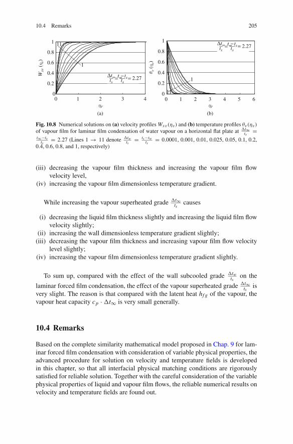
10.4 Remarks 205
0
0.2
0.4
0.6
0.8
1
ηv
1
11
(a)
0 1 2 3 40
0.2
0.4
0.6
0.8
1
0 1 2 3 4 5 6ηv
1
11
(b)
θ v (
η v)
Wxv
(η v
)
= 2.27=Δt∞ts ts
− tst∞
= 2.27=Δt∞ts ts
− tst∞
Fig. 10.8 Numerical solutions on (a) velocity profiles Wxv(ηv) and (b) temperature profiles θv(ηv)of vapour film for laminar film condensation of water vapour on a horizontal flat plate at �t∞
ts=
t∞−tsts
= 2.27 (Lines 1 → 11 denote �twts
= ts−twts
= 0.0001, 0.001, 0.01, 0.025, 0.05, 0.1, 0.2,0.4, 0.6, 0.8, and 1, respectively)
(iii) decreasing the vapour film thickness and increasing the vapour film flowvelocity level,
(iv) increasing the vapour film dimensionless temperature gradient.
While increasing the vapour superheated grade �t∞ts
causes
(i) decreasing the liquid film thickness slightly and increasing the liquid film flowvelocity slightly;
(ii) increasing the wall dimensionless temperature gradient slightly;(iii) decreasing the vapour film thickness and increasing vapour film flow velocity
level slightly;(iv) increasing the vapour film dimensionless temperature gradient slightly.
To sum up, compared with the effect of the wall subcooled grade �twts
on the
laminar forced film condensation, the effect of the vapour superheated grade �t∞ts
isvery slight. The reason is that compared with the latent heat hf g of the vapour, thevapour heat capacity cp ·�t∞ is very small generally.
10.4 Remarks
Based on the complete similarity mathematical model proposed in Chap. 9 for lam-inar forced film condensation with consideration of variable physical properties, theadvanced procedure for solution on velocity and temperature fields is developedin this chapter, so that all interfacial physical matching conditions are rigorouslysatisfied for reliable solution. Together with the careful consideration of the variablephysical properties of liquid and vapour film flows, the reliable numerical results onvelocity and temperature fields are found out.

206 10 Velocity and Temperature Fields
Increasing the wall subcooled grade �twts
causes increasing the liquid film thick-ness ηl,δ and interfacial velocities, decreasing wall dimensionless temperature gra-dient, decreasing the vapour film thickness, increasing the vapour film flow velocitylevel, and increasing the vapour film dimensionless temperature gradient.
Increasing the vapour superheated grade �t∞ts
causes decreasing the liquid filmthickness slightly, increasing the liquid velocity slightly, increasing the wall dimen-sionless temperature gradient slightly, decreasing the vapour film thickness, increas-ing vapour film flow velocity level, and increasing the vapour film dimensionlesstemperature gradient.
Compared with the effect of the wall subcooled grade �twts
on the laminar forced
film condensation, the effect of the vapour superheated grade �t∞ts
is very slight.The reason is that compared with the latent heat hf g of the vapour, the vapour heatcapacity cp · �t∞ is very small generally. All these express the coupled effectsof the variable physical properties of vapour and liquid on the laminar forced filmcondensation.
It should be emphasized that satisfying all interfacial physical matching con-ditions is important for obtaining reliable solutions for the laminar forced filmcondensation with two-phase flows. Even one of the interfacial physical matchingconditions is ignored, the solutions will be multiple, and it is never possible to obtainthe sole set of correct solutions.
Exercises
1. From the numerical results on velocity and temperature fields of laminar forcedfilm condensation of vapour reported in this chapter, it is seen the obvious cou-pled effects of variable physical properties on the laminar forced film condensa-tion. Please point out the correct meaning of “the coupled effects”.
2. Please indicate all liquid–vapour interfacial matching conditions of laminarforced film condensation of vapour and explain why all these interfacial match-ing conditions should be satisfied for a reliable solution.
References
1. D.Y. Shang, B.X. Wang, Effect of variable thermophysical properties on laminar free convec-tion of gas. Int. J. Heat Mass Transfer 33(7), 1387–1395 (1990)
2. D.Y. Shang, B.X. Wang, Effect of variable thermophysical properties on laminar free convec-tion of polyatomic gas. Int. J. Heat Mass Transfer 34(3) 749–755 (1991)
3. D.Y. Shang, Free Convection Film Flows and Heat Transfer (Springer, Berlin, Heidelberg andNew York, NY, 2006)
4. D.Y. Shang, B.X. Wang, Y. Wang, Y. Quan, Study on liquid laminar free convection withconsideration of variable thermophysical properties. Int. J. Heat Mass Transfer 36(14), 3411–3419 (1993)

References 207
5. D.Y. Shang, T. Adamek, Study on laminar film condensation of saturated steam on a verti-cal flat late for consideration of various physical factors including variable thermophysicalproperties. Warme- und Stoffubertragung 30(2), 89–100 (1994)
6. D.Y. Shang, B.X. Wang, An extended study on steady-state laminar film condensation of asuperheated vapor on an isothermal vertical plate. Int. J. Heat Mass Transfer 40(4), 931–941(1997)


Chapter 11Heat and Mass Transfer on Laminar ForcedFilm Condensation of Pure Vapour
Abstract On the basis of Chaps. 9 and 10, heat and mass transfer investigation isdone under the new similarity analysis system for laminar forced film condensationof pure vapour. The heat transfer analysis equations are provided where the walldimensionless temperature gradient becomes only one no-given variable for predic-tion of condensate heat transfer. By means of the condensate mass transfer analysis,the condensate mass flow rate parameter is induced as the function of the dimension-less condensate liquid film thickness and the interfacial dimensionless condensateliquid velocity components. It is found that the condensate mass flow rate parameteris the only one no-given variable for prediction of condensate mass transfer. Takethe laminar forced film condensation of water vapour on a horizontal flat plate as anexample, the systems of key numerical solutions on the wall dimensionless tempera-ture gradient and mass flow rate parameter is obtained, and further rigorously formu-lated by using curve-fitting approach. With the rigorously formulated equations onthe wall dimensionless temperature gradient and mass flow rate parameter, the theo-retical analysis equations on condensate heat and mass become available for simpleand reliable prediction of heat and mass transfer on laminar forced film condensationof saturated and superheated water vapour. Thus, the effects of the wall subcooledgrade and vapour superheated grads on the condensate heat and mass transfer areclarified. Although increasing the wall subcooled grade causes decreasing the walltemperature gradient, it will increase the condensate heat transfer. Increasing thewall subcooled grade causes increasing the condensate mass flow rate parameter,and further causes increasing the condensate mass flow rate. Increasing the vapoursuperheated grade causes decreasing the condensate mass flow rate parameter, andfurther causes decreasing the condensate mass flow rate. Compared with the effectof the wall subcooled grade on heat and mass transfer of the forced film conden-sation, the effect of the vapour subcooled grade is so slight that it can be ignoredin the special range of the superheated grade. At last, a condensate mass–energytransformation equation is reported in this chapter under the new similarity analysissystem for a better clarification of the internal relation of film condensate heat andmass transfer.
D.Y. Shang, Theory of Heat Transfer with Forced Convection Film Flows,Heat and Mass Transfer, DOI 10.1007/978-3-642-12581-2_11,C© Springer-Verlag Berlin Heidelberg 2011
209
210 11 Heat and Mass Transfer on Laminar Forced Film Condensation of Pure Vapour
11.1 Introduction
On the basis of Chaps. 9 and 10, respectively, for complete similarity mathematicalmodel and the numerical results of velocity and temperature fields, in this chapterfurther investigation will be done for heat and mass transfer of laminar forced filmcondensation of pure vapour. First, the appropriate heat transfer analysis will bedone for providing the appropriate heat transfer theoretical equations in which thekey solution, i.e. the wall dimensionless temperature gradient, will dominate con-densate heat and mass transfer. Meanwhile, the condensate mass flow rate param-eter will be induced by the mass transfer analysis, which will be the function ofthe dimensionless liquid film thickness, as well as the condensate interfacial veloc-ity components, and will dominate condensate mass transfer. Furthermore, the keysolutions on the wall dimensionless temperature gradient and the condensate massflow rate parameter of the similarity governing mathematical model will be formu-lated based on the rigorous numerical results, so that the theoretical equations oncondensate heat and mass transfer can be conveniently used for simple and reliableprediction. In addition, the mass-energy transformation equation is reported in thischapter for description of the transformation relation between the key solutions, i.e.the wall temperature gradient and the mass flow rate parameter, which dominate thecondensate mass and heat transfer, respectively.
11.2 Condensate Heat Transfer Analysis
In the previous chapters, the heat transfer analysis was done for laminar forcedconvection, while the following heat and mass transfer analysis is for laminar forcedfilm condensation.
The local heat transfer rate qx,w of the film condensation at position x per unit
area on the plate can be calculated by applying Fourier’s law as qx = −λl,w
(∂t∂y
)y=0
with consideration of variable physical properties. With the assumed transformationvariable of (9.14), (9.15), and (9.16) for liquid film, qx,w is described as
qx,w = λl,w(tw − ts)
(1
2Rexl,s
)1/2
x−1(
−dθl(ηl)
dηl
)
ηl=0. (11.1)
Then the local heat transfer coefficient, defined as qx,w = αx,w(tw − ts), will be
αx,w = λl,w
(1
2Rexl,s
)1/2
x−1(
−dθl(ηl)
dηl
)
ηl=0. (11.2)

11.2 Condensate Heat Transfer Analysis 211
The local Nusselt number, defined as Nuxl,w = αx,wx
λl,w, is expressed by
Nuxl,w =(
1
2Rexl,s
)1/2 (−dθl(ηl)
dηl
)
ηl=0. (11.3)
The total heat transfer rate for position x = 0 to x with width of b on the plate is anintegration
Qx,w =∫∫
Aqx,wdA =
∫ x
0qx,wb dx,
where the plate condensate heat transfer area is described as A = b × x , where b isthe plate width related to heat transfer.
With (11.1), the above equation is changed to
Qx,w =∫ x
0bλl,w(tw − ts)
(1
2Rexl,s
)1/2
x−1(
−dθl(ηl)
dηl
)
ηl=0dx .
With definition of local Reynolds number Rexl,s in (9.15), we obtain
Qx,w = √2bλl,w(tw − ts)(Rexl,s)
1/2(
−dθl(ηl)
dηl
)
ηl=0. (11.4)
The average heat transfer coefficient αx,w defined as Qx,w = αx,w(tw − ts)A isexpressed as
αx,w = 2λl,w
(1
4Rexl,s
)1/2
x−1(
−dθl(ηl)
dηl
)
ηl=0. (11.5)
The average Nusselt number defined as Nuxl,w = αx,wx
λl,wwill be
Nuxl,w = √2(Rexl,s)
1/2(
−dθl(ηl)
dηl
)
ηl=0. (11.6)
Here, it is necessary to mention the positive and negative signs for heat transferresults of the film condensation, such as those found out in (11.1) and (11.4). In fact,the value of the dimensionless temperature gradient is negative, and the temperature
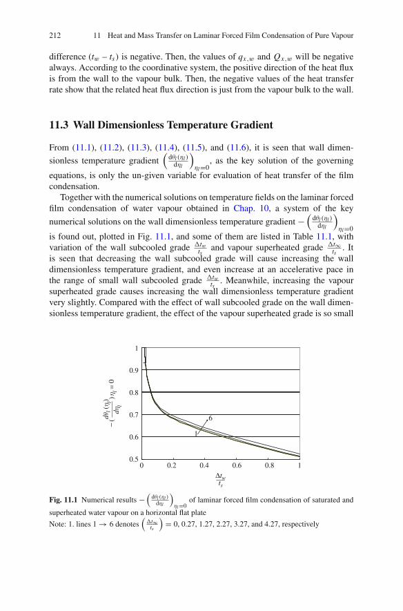
212 11 Heat and Mass Transfer on Laminar Forced Film Condensation of Pure Vapour
difference (tw – ts) is negative. Then, the values of qx,w and Qx,w will be negativealways. According to the coordinative system, the positive direction of the heat fluxis from the wall to the vapour bulk. Then, the negative values of the heat transferrate show that the related heat flux direction is just from the vapour bulk to the wall.
11.3 Wall Dimensionless Temperature Gradient
From (11.1), (11.2), (11.3), (11.4), (11.5), and (11.6), it is seen that wall dimen-
sionless temperature gradient(
dθl(ηl )dηl
)ηl=0
, as the key solution of the governing
equations, is only the un-given variable for evaluation of heat transfer of the filmcondensation.
Together with the numerical solutions on temperature fields on the laminar forcedfilm condensation of water vapour obtained in Chap. 10, a system of the key
numerical solutions on the wall dimensionless temperature gradient −(
dθl (ηl )dηl
)ηl=0
is found out, plotted in Fig. 11.1, and some of them are listed in Table 11.1, withvariation of the wall subcooled grade �tw
tsand vapour superheated grade �t∞
ts. It
is seen that decreasing the wall subcooled grade will cause increasing the walldimensionless temperature gradient, and even increase at an accelerative pace inthe range of small wall subcooled grade �tw
ts. Meanwhile, increasing the vapour
superheated grade causes increasing the wall dimensionless temperature gradientvery slightly. Compared with the effect of wall subcooled grade on the wall dimen-sionless temperature gradient, the effect of the vapour superheated grade is so small
0.5
0.6
0.7
0.8
0.9
1
0 0.2 0.4 0.6 0.8 1
1
6
tsΔtw
)(
−dη
l
dθl (
η l)η l =
0
Fig. 11.1 Numerical results −(
dθl (ηl )dηl
)ηl =0
of laminar forced film condensation of saturated and
superheated water vapour on a horizontal flat plate
Note: 1. lines 1 → 6 denotes(�t∞
ts
)= 0, 0.27, 1.27, 2.27, 3.27, and 4.27, respectively

11.4 Prediction Equations on Heat Transfer 213
that it can be ignored within the range of 0 ≤ �t∞ts
≤ 4.27 without any obviousinfluence caused on condensate heat transfer prediction. According to such analy-sis, by using a curve-fitting approach, the system of numerical solutions on the walldimensionless temperature gradient for laminar forced film condensation of watervapour along a horizontal flat plate is formulated to the following equations:
for 0 ≤ �t∞ts
≤ 4.27
−(
dθl(ηl)
dηl
)
ηl=0=
0.7421�tw
ts+ 0.3124
(�tw
ts
)0.28 (0.01 ≤ �twts
≤ 0.1) (11.7)
−(
dθl(ηl)
dηl
)
ηl=0= 0.1466
(�tw
ts
)2
− 0.3974
(�tw
ts
)
+ 0.7652
(0.1 ≤ �tw
ts≤ 1
)(11.8)
The results on the wall dimensionless temperature gradient(
dθl (ηl )dηl
)ηl=0
predicted
by using (11.7) and (11.8) are listed in Table 11.1. It is seen that the predictiondeviation of (11.7) is less than 0.47% for �t∞
ts= 0, and less than 0.87% for 0 <
�t∞ts
≤ 4.27, while the prediction deviation of (11.8) is less than 1.48% for �t∞ts
= 0,
and less than 3.32% for 0 < �t∞ts
≤ 4.27. These predicted results are well coincident
to the related numerical results for 0 ≤ �t∞ts
≤ 4.27.Obviously, (11.7) and (11.8) are suitable for laminar forced film condensation of
water vapour on a horizontal flat plate.
11.4 Prediction Equations on Heat Transfer
Combined with the formulated equations (11.7) and (11.8), the theoretical analy-sis equations (11.1) to (11.6) on heat transfer become available for prediction ofthe condensate heat transfer results. For example, combined with the formulatedequations (11.7) and (11.8), (11.4) and (11.6) are changed to the following equa-tions for prediction of the heat transfer result and average Nusselt number within�t∞
ts≤ 4.27 for laminar forced film condensation of water vapour on the horizontal
flat plate.

214 11 Heat and Mass Transfer on Laminar Forced Film Condensation of Pure Vapour
Tabl
e11
.1N
umer
ical
resu
lts−(dθ l(η
l)/dη
l)η
l=
0of
lam
inar
forc
edfil
mco
nden
satio
nof
satu
rate
dan
dsu
perh
eate
dw
ater
vapo
uron
aho
rizo
ntal
flat
plat
e(a
deno
tes
num
eric
also
lutio
ns,b
deno
tes
pred
icte
dva
lues
byus
ing
(11.
7)an
d(1
1.8)
,and
cde
note
spr
edic
ted
devi
atio
n)�
t w t s
0.01
0.02
50.
050.
10.
20.
40.
60.
81
�t ∞ t s
−( dθ
ldη
l
) ηl=
0
0a
1.15
90.
9285
020.
8124
50.
7353
442
0.68
1475
0.62
6769
0.58
3673
0.54
5086
0.51
1398
7b
1.16
120.
9296
990.
8086
150.
7366
700.
6915
840.
6296
960.
5795
360.
5411
040.
5144
c−0.0
019
−0.0
0129
0.00
472
−0.0
0180
0.01
4834
0.00
467
−0.0
0709
−0.0
0731
0.00
5869
00.2
7a
1.15
9739
0.92
8717
0.81
2572
0.73
5451
80.
6814
960.
6267
720.
5836
730.
5450
850.
5114
84b
1.16
120.
9296
990.
8086
150.
7366
700.
6890
890.
6374
590.
5896
980 .
5455
150.
5046
42c
−0.0
0126
−0.0
0106
0.00
487
−0.0
0165
0.01
4803
0.00
4665
−0.0
0709
−0.0
073
0.00
5701
10.2
7a
1.16
0344
0.92
9191
0.81
2921
0.73
5613
20.
6815
610.
6267
720.
5836
730.
5450
980.
5114
841
b1.
1612
0.92
9699
0.80
8615
0.73
6670
0.69
1584
0.62
9696
0.57
9536
0.54
1104
0.51
44c
−0.0
0074
−0.0
0055
0.00
5297
−0.0
0143
0.01
4706
0.00
4665
−0.0
0709
−0.0
0733
0.00
5701
20.2
7a
1.16
1017
0.92
964
0.81
3231
0.73
5882
50.
6816
80.
6269
820.
5838
990.
5453
850.
5118
526
b1.
1612
0.92
9699
0.80
8615
0.73
6670
0.69
1584
0.62
9696
0.57
9536
0.54
1104
0.51
44c
−0.0
0016
−6.4
E–0
50.
0056
76−0.0
0107
00.
0145
290.
0043
29−0.0
0747
−0.0
0785
0.00
4977
30.2
7a
1.16
1584
0.93
0098
0.81
3694
0.73
6962
10.
6848
280.
6315
210.
5890
090.
5494
640.
5156
593
b1.
1612
0.92
9699
0.80
8615
0.73
6670
0.69
1584
0.62
9696
0.57
9536
0.54
1104
0.51
44c
0.00
0331
0.00
0428
0.00
6241
0.00
0396
0.00
9865
0.00
4329
−0.0
0747
−0.0
0785
0.00
4977
40.2
7a
1.16
219
0.93
0711
0.81
5574
0.74
3098
70.
6943
970.
6424
790.
5991
850.
5596
60.
5255
988
b1.
1612
0.92
9699
0.80
8615
0.73
6670
0.69
1584
0.62
9696
0.57
9536
0.54
1104
0.51
44c
0.00
0852
0.00
1087
0.00
8533
0.00
8650
−0.0
0405
−0.0
199
−0.0
3279
−0.0
3316
−0.0
2131
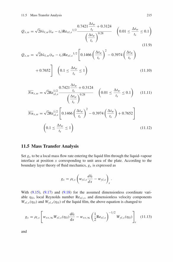
11.5 Mass Transfer Analysis 215
Qx,w = √2bλl,w(tw − ts)Rexl,s
1/20.7421
�twts
+ 0.3124
(�tw
ts
)0.28
(0.01 ≤ �tw
ts≤ 0.1
)
(11.9)
Qx,w = √2bλl,w(tw − ts)Rexl,s
1/2
[0.1466
(�tw
ts
)2
− 0.3974
(�tw
ts
)
+ 0.7652
] (0.1 ≤ �tw
ts≤ 1
)(11.10)
Nux,w = √2Re1/2
xl,s
0.7421�tw
ts+ 0.3124
(�tw
ts
)0.28
(0.01 ≤ �tw
ts≤ 0.1
)(11.11)
Nux,w = √2Re1/2
xl,s
[0.1466
(�tw
ts
)2
− 0.3974
(�tw
ts
)+ 0.7652
]
(0.1 ≤ �tw
ts≤ 1
)(11.12)
11.5 Mass Transfer Analysis
Set gx to be a local mass flow rate entering the liquid film through the liquid–vapourinterface at position x corresponding to unit area of the plate. According to theboundary layer theory of fluid mechanics, gx is expressed as
gx = ρl,s
(wxl,s
dδldx
− wyl,s
)
s.
With (9.15), (9.17) and (9.18) for the assumed dimensionless coordinate vari-able ηlδ , local Reynolds number Rexl,s , and dimensionless velocity componentsWxl,s(ηlδ) and Wyl,s(ηlδ) of the liquid film, the above equation is changed to
gx = ρl,s
[wxv,∞Wxl,s(ηlδ)
dδldx
− wxv,∞(
1
2Rexl,s
)−1/2
Wyl,s(ηlδ)
]
s
(11.13)
and

216 11 Heat and Mass Transfer on Laminar Forced Film Condensation of Pure Vapour
δl = ηlδ
(1
2
wxv,∞x
νl,s
)−1/2
x,
dδldx
= 1
2ηlδ
(1
2Rexl,s
)−1/2
. (11.14)
With (11.14), (11.13) is changed to
gx = ρl,s
[wxv,∞Wxl,s(ηlδ)
1
2ηlδ,s
(1
2Rexl,s
)−1/2
−wxv,∞(
1
2Rexl,s
)−1/2
Wyl,s(ηlδ)
],
i.e.
gx = 1
2ρl,swxv,∞
(1
2Rexl,s
)−1/2
[ηlδ,s Wxl,s(ηlδ)− 2Wyl,s(ηlδ)].
The above equation is rewritten as
gx = 1
2ρl,swxv,∞
(1
2Rexl,s
)−1/2
�s, (11.15)
where �s can be defined as mass flow rate parameter of laminar forced film con-densation with the following expression:
�s = ηlδ · Wxl,s(ηlδ)− 2Wyl,s(ηlδ). (11.16)
Take Gx to express total mass flow rate entering the liquid film through the liquid–vapour interface from position x = 0 to x with width of b of the plate, it should bethe following integration:
Gx =∫∫
A
gx d A = b∫ x
0gx dx,
where A = b · x is related area of the plate with b as the plate width correspondingto the condensation.
With (11.15), the above equation is changed to
Gx = 1
2b∫ x
0ρl,swxv,∞
(1
2Rexl,s
)−1/2
�sdx .
With the definition of Rexl,s , the above equation is changed to

11.6 Mass Flow Rate Parameter 217
Gx = 1
2b∫ x
0ρl,swxv,∞
(1
2
wxv,∞x
νl,s
)−1/2
�sdx .
Then
Gx = 2 · 1
2bρl,swxv,∞x1/2
(1
2
wxv,∞νl,s
)−1/2
�s,
i.e.
Gx = 2bρl,sνl,s
(1
2
wxv,∞x
νl,s
)1/2
�s,
or
Gx = √2bμl,sRexl,s
1/2�s . (11.17)
Obviously, (11.16) and (11.17) are universally suitable for general laminar forcedfilm condensation.
11.6 Mass Flow Rate Parameter
From (11.15) and (11.17), it is seen that the condensate mass flow rate para-meter �s , as the key solution of the governing equations, is only the un-givenvariable for evaluation of the condensate mass flow rate of the laminar forced filmcondensation. In this case, the evaluation of the condensate mass flow rate parameteris necessary for calculation of the condensate mass flow rate.
Equation (11.16) demonstrates that the condensate mass flow rate parameter�s is the function of the key solutions on dimensionless liquid film thickness ηlδ ,and dimensionless interfacial liquid velocity components Wxl,s(ηlδ) and Wyl,s(ηlδ).Then, first it is necessary to investigate the variation regulations of these key solu-tions.
The rigorous key numerical solutions for dimensionless condensate film thick-ness ηlδ , and the interfacial dimensionless liquid velocity components Wxl,s(ηlδ)
and Wyl,s(ηlδ), obtained together with the solutions in Chap. 10 are plotted inFigs. 11.2, 11.3, and 11.4 and some of their values are listed in Tables 11.2, 11.3,and 11.4, respectively. Then, a system of solutions on the condensate mass flow rateparameter�s found out with (11.16) are plotted in Fig. 11.5 and listed in Table 11.5.From these numerical results, the following points should be addressed.
Decreasing the wall subcooled grade causes decreasing the condensate liquidfilm thickness. In the range of small wall subcooled grade, the condensate liquidfilm thickness will decrease at an accelerative pace with decreasing the wall sub-cooled grade. In addition, increasing the wall subcooled grade will causes increas-ing the interfacial dimensionless condensate liquid velocity component Wyl,s(ηlδ)
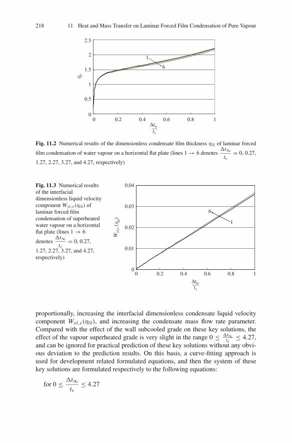
218 11 Heat and Mass Transfer on Laminar Forced Film Condensation of Pure Vapour
0
0.5
1
1.5
2
2.5
0 0.2 0.4 0.6 0.8 1
1
6
η lδ
ts
Δtw
Fig. 11.2 Numerical results of the dimensionless condensate film thickness ηlδ of laminar forced
film condensation of water vapour on a horizontal flat plate (lines 1 → 6 denotes�t∞
ts= 0, 0.27,
1.27, 2.27, 3.27, and 4.27, respectively)
Fig. 11.3 Numerical resultsof the interfacialdimensionless liquid velocitycomponent Wyl,s (ηlδ) oflaminar forced filmcondensation of superheatedwater vapour on a horizontalflat plate (lines 1 → 6
denotes�t∞
ts= 0, 0.27,
1.27, 2.27, 3.27, and 4.27,respectively)
0
0.01
0.02
0.03
0.04
0 0.2 0.4 0.6 0.8 1
tsΔtw
1
6
Wyl
,s (
η lδ)
proportionally, increasing the interfacial dimensionless condensate liquid velocitycomponent Wxl,s(ηlδ), and increasing the condensate mass flow rate parameter.Compared with the effect of the wall subcooled grade on these key solutions, theeffect of the vapour superheated grade is very slight in the range 0 ≤ �t∞
ts≤ 4.27,
and can be ignored for practical prediction of these key solutions without any obvi-ous deviation to the prediction results. On this basis, a curve-fitting approach isused for development related formulated equations, and then the system of thesekey solutions are formulated respectively to the following equations:
for 0 ≤ �t∞ts
≤ 4.27

11.6 Mass Flow Rate Parameter 219
Tabl
e11
.2N
umer
ical
resu
ltsη
lδof
lam
inar
forc
edfil
mco
nden
satio
nof
wat
erva
pour
ona
hori
zont
alfla
tpla
te�
t w t s 0.01
0.02
50.
050.
10.
20.
40.
60.
81
�t ∞ t s
ηlδ
0a
0.86
277
1.07
815
1.23
3585
1.36
651.
484
1.64
235
1.80
782.
0001
2.22
35b
0.87
8334
1.05
5665
1.21
3230
1.39
0224
1.46
5073
1.62
7077
1.80
6995
2.00
6808
2.22
8715
c0.
0180
−0.0
208
−0.0
1659
0.01
736
−0.0
127
−0.0
093
−0.0
0044
0.00
335
0.00
234
0.27
a0.
8626
21.
0779
1.23
341.
3663
1.48
395
1.64
235
1.80
782.
0001
2.22
31b
0.87
8334
1.05
5665
1.21
3230
1.39
0224
1.46
5073
1.62
7077
1.80
6995
2.00
6808
2.22
8716
c0.
0182
−0.0
206
−0.0
163
0.01
751
−0.0
127
−0.0
093
−0.0
0044
0.00
335
0.00
2526
1.27
a0.
8621
71.
0773
51.
2328
71.
366
1.48
381
1.64
235
1.80
782.
0000
52.
2231
b0.
8783
341.
0556
651.
2132
301.
3902
241.
4650
731.
6270
771.
8069
952.
0068
082.
2287
16c
0.01
874
−0.0
2012
−0.0
159
0.01
773
−0.0
126
−0.0
093
−0.0
0044
0.00
338
0.00
2526
2.27
a0.
8616
71.
0768
31.
2324
1.36
551.
4835
51.
6418
1.80
711.
999
2.22
15b
0.87
8334
1.05
5665
1.21
3230
1.39
0224
1.46
5073
1.62
7077
1.80
6995
2.00
6808
2.22
8716
c0.
0193
4−0.0
196
−0.0
155
0.01
81−0.0
1245
−0.0
089
−5.7
85E
–05
0.00
390
0.00
3248
3.27
a0.
8612
51.
0763
1.23
171.
3635
1.47
673
1.63
1.79
1421
1.98
416
2.20
51b
0.87
8334
1.05
5665
1.21
3230
1.39
0224
1.46
5073
1.62
7077
1.80
6995
2.00
6808
2.22
8716
c0.
0198
−0.0
1917
−0.0
1499
0.01
960
−0. 0
0789
−0.0
0179
0.00
869
0.01
141
0.01
0709
4.27
a0.
8608
1.07
559
1.22
886
1.35
224
1.45
638
1.60
221.
761
1.94
801
2.16
34b
0.87
8334
1.05
5665
1.21
3230
1.39
0224
1.46
5073
1.62
7077
1.80
6995
2.00
6808
2.22
8716
c0.
0203
7−0.0
185
−0.0
1271
90.
0280
90.
0059
70.
0155
0.02
610.
0301
80.
0301
91

220 11 Heat and Mass Transfer on Laminar Forced Film Condensation of Pure Vapour
Tabl
e11
.3N
umer
ical
resu
ltsW
yl,s(η
lδ)
ofla
min
arfo
rced
film
cond
ensa
tion
ofsu
perh
eate
dw
ater
vapo
uron
aho
rizo
ntal
flatp
late
�t w t s 0.
010.
025
0.05
0.1
0.2
0.4
0.6
0.8
1
�t ∞ t s
Wyl,s(η
lδ)
0a
0.00
062
0.00
1245
0.00
2187
0.00
3994
0.00
7547
0.01
450.
0214
170.
0284
250.
0356
95b
0.00
0643
0.00
1202
50.
0021
350.
0039
930.
0075
360.
0146
220.
0217
080.
0287
940.
0358
8c
0.03
71−0.0
341
−0.0
238
−0.0
0025
−0.0
0146
0.00
841
0.01
360.
013
0.00
518
0.27
a0.
0006
20.
0012
450.
0021
870.
0039
937
0.00
7543
0.01
4514
0.02
1419
0.02
8419
0.03
5649
b0.
0006
430.
0012
025
0.00
2135
0.00
3993
0.00
7536
0.01
4622
0.02
1708
0.02
8794
0 .03
588
c0.
0371
−0.0
341
−0.0
238
−0.0
0018
−0.0
0093
0.00
740.
0135
0.01
320.
0064
8
1.27
a0.
0006
210.
0012
450.
0021
880.
0039
950.
0075
440.
0145
140.
0214
190.
0284
20.
0356
50b
0.00
0643
0.00
1202
50.
0021
350.
0039
930.
0075
360.
0146
220.
0217
080.
0287
940.
0358
8c
0.03
54−0.0
341
−0.0
242
−0.0
005
−0.0
0106
0.00
744
0.01
349
0.01
316
0.00
645
2.27
a0.
0006
210.
0012
460.
0021
890 .
0039
960.
0075
450.
0145
190.
0214
280.
0284
350.
0356
76b
0.00
0643
0.00
1202
50.
0021
350.
0039
930.
0075
360.
0146
220.
0217
080.
0287
940.
0358
8c
0.03
54−0.0
349
−0.0
246
−0.0
0075
−0.0
0119
0.00
709
0.01
30.
0126
0.00
5718
3.27
a0.
0006
210.
0012
470.
0021
90.
0040
020.
0075
80.
0146
240.
0216
150.
0286
480.
0359
41b
0.00
0643
0.00
1202
50.
0021
350.
0039
930.
0075
360.
0146
220.
0217
080.
0287
940.
0358
8c
0.03
54−0.0
357
−0.0
251
−0.0
0225
−0.0
058
−0.0
0014
0.00
430.
0050
96−0.0
017
4.27
a0.
0006
220.
0012
470.
0021
950.
0040
350.
0076
860.
0148
780.
0219
890.
0291
80.
0366
34b
0.00
0643
0.00
1202
50.
0021
350.
0039
930.
0075
360.
0146
220.
0217
080.
0287
940.
0358
8c
0.03
376
−0.0
357
−0.0
273
−0.0
104
−0.0
195
−0.0
172
−0.0
128
−0.0
132
−0.0
206

11.6 Mass Flow Rate Parameter 221
Tabl
e11
.4N
umer
ical
resu
ltsW
xl,s(η
lδ)
ofla
min
arfo
rced
film
cond
ensa
tion
ofsu
perh
eate
dw
ater
vapo
uron
aho
rizo
ntal
flatp
late
�t w t s 0.
010.
025
0.05
0.1
0.2
0.4
0.6
0.8
1
�t ∞ t s
Wxl,s(η
lδ)
0a
0.00
2871
0.00
4603
0.00
7042
0.01
1522
0.01
9724
0.03
295
0.04
225
0.04
8175
0.05
16b
0.00
2991
0.00
4418
0.00
6795
0.01
226
0.01
990.
0327
20.
0422
60.
0485
20.
0515
c0.
0418
−0.0
403
−0.0
351
0.06
405
0.00
89−0.0
0698
0.00
0237
0.00
716
−0.0
0194
0.27
a0.
0028
70.
0046
030.
0070
440.
0115
240.
0197
140.
0329
80.
0422
530.
0481
650.
0515
45b
0.00
2991
0.00
4418
0.00
6795
0.01
226
0.01
990.
0327
20.
0422
60.
0485
20 .
0515
c0.
0421
6−0.0
403
−0.0
3535
0.06
389
0.00
943
−0.0
0788
0.00
0165
0.00
737
−0.0
0087
1.27
a0.
0028
750.
0046
080.
0070
50.
0115
290.
0197
180.
0329
810.
0422
540.
0481
690.
0515
47b
0.00
2991
0.00
4418
0.00
6795
0.01
226
0.01
990.
0327
20.
0422
60.
0485
20.
0515
c0.
0403
−0.0
413
−0.0
3617
0.06
340.
0092
3−0.0
0791
0.00
0142
0.00
7287
−0.0
0091
2.27
a0.
0028
790.
0046
130.
0070
550 .
0115
380.
0197
250.
0330
030.
0422
870.
0482
190.
0516
21b
0.00
2991
0.00
4418
0.00
6795
0.01
226
0.01
990.
0327
20.
0422
60.
0485
20.
0515
c0.
0389
−0.0
4238
−0.0
3685
0.06
260.
0088
7−0.0
0857
−0.0
0065
0.00
624
−0.0
0234
3.27
a0.
0028
810.
0046
170.
0070
630.
0115
720.
0199
080.
0334
830.
0430
310.
0489
430.
0523
92b
0.00
2991
0.00
4418
0.00
6795
0.01
226
0.01
990.
0327
20.
0422
60.
0485
20.
0515
c0.
0381
8−0.0
432
−0.0
3794
0.05
949
−0.0
004
−0.0
2279
−0.0
179
−0.0
0864
−0.0
17
4.27
a0.
0028
840.
0046
230.
0070
960.
0117
650.
0204
680.
0346
550.
0445
30.
0507
770.
0544
31b
0.00
2991
0.00
4418
0.00
6795
0.01
226
0.01
990.
0327
20.
0422
60.
0485
20.
0515
c0.
0371
−0.0
4445
−0.0
424
0.04
207
−0.0
2775
−0.0
558
−0.0
5098
−0.0
4445
−0.0
5385

222 11 Heat and Mass Transfer on Laminar Forced Film Condensation of Pure Vapour
Fig. 11.4 Numerical resultsof the interfacialdimensionless liquid velocitycomponent Wxl,s(ηlδ) oflaminar forced filmcondensation of superheatedwater vapour on a horizontalflat plate ( lines 1 → 6
denotes�t∞
ts= 0, 0.27,
1.27, 2.27, 3.27, and 4.27,respectively)
0
0.01
0.02
0.03
0.04
0.05
0.06
0 0.2 0.4 0.6 0.8 1
1
6
ts
Δtw
Wxl
, s(η
lδ)
Fig. 11.5 Numerical resultsof condensate mass flow rateparameter �s of laminarforced film condensation ofsuperheated water vapour ona horizontal flat plateNote: 1. lines 1 → 6 denotes�t∞
ts= 0, 0.27, 1.27, 2.27,
3.27, and 4.27, respectively
0
0.01
0.02
0.03
0.04
0.05
0 0.2 0.4 0.6 0.8 1
Φs
1
6
tsΔtw
ηlδ = 2.2134
(�tw
ts
)0.2007 (0.01 ≤ �tw
ts≤ 0.1
)(11.18)
ηlδ = 1.3192 exp
(0.5244
(�tw
ts
)) (0.1 ≤ �tw
ts≤ 1
)(11.19)
Wyl,s(ηlδ) = 0.0373
(�tw
ts
)+ 0.00027
(0.01 ≤ �tw
ts≤ 0.1
)(11.20)
Wyl,s(ηlδ) = 0.03543
(�tw
ts
)+ 0.00045
(0.1 ≤ �tw
ts≤ 1
)(11.21)
Wxl,s(ηlδ) = 0.0951
(�tw
ts
)+ 0.00204
(0.01 ≤ �tw
ts≤ 0.1
)(11.22)

11.6 Mass Flow Rate Parameter 223
Tabl
e11
.5N
umer
ical
resu
lts�
sof
lam
inar
forc
edfil
mco
nden
satio
nof
supe
rhea
ted
wat
erva
pour
ona
hori
zont
alfla
tpla
te�
t w t s 0.01
0.02
50.
050.
10.
20.
40.
60.
81
�t ∞ t s
�s
0a
0.00
1237
0.00
2473
0.00
4313
0.00
7757
50.
0141
760.
0251
150.
0335
450.
0395
060.
0433
42b
0.00
1289
0.00
2367
50.
0041
650.
0077
490.
0140
960.
0249
840.
0334
640.
0395
360.
0432
c0.
042
−0.0
4266
−0.0
343
−0.0
011
−0.0
0564
−0.0
052
−0.0
0241
0.00
0759
−0.0
0328
0.27
a0.
0012
370.
0024
720.
0043
130.
0077
580.
0141
680.
0251
380.
0335
470.
0394
970.
0432
92b
0.00
1289
0.00
2367
50.
0041
650.
0077
490.
0140
960.
0249
840.
0334
640.
0395
360.
0432
c0.
042
−0.0
4227
−0.0
343
−0.0
011
−0.0
0508
−0.0
0613
−0.0
0247
0.00
0987
−0.0
0213
1.27
a0.
0012
380.
0024
740.
0043
150.
0077
600.
0141
70.
0251
380.
0335
480.
0394
990.
0432
93b
0.00
1289
0.00
2367
50.
0041
650.
0077
490.
0140
960.
0249
840.
0334
640.
0395
360.
0432
c0.
0412
−0.0
43−0.0
3476
−0.0
0135
−0.0
0522
−0.0
0613
−0.0
025
0.00
0937
−0.0
0215
2.27
a0.
0012
390.
0024
750.
0043
170.
0077
620.
0141
730.
0251
470.
0335
610.
0395
20.
0433
24b
0.00
1289
0.00
2367
50.
0041
650.
0077
490.
0140
960.
0249
840.
0334
640.
0395
360.
0432
c0.
0403
6−0.0
434
−0.0
3521
−0.0
0167
−0.0
054
−0.0
0648
−0.0
0289
0.00
0405
−0.0
0286
3.27
a0.
0012
390.
0024
760.
0043
190.
0077
740.
0142
380.
0253
290.
0338
550.
0398
160.
0436
47b
0.00
1289
0.00
2367
50.
0041
650.
0077
490.
0140
960.
0249
840.
0334
640.
0395
360.
0432
c0.
0403
6−0.0
438
−0.0
356
−0.0
0319
−0.0
0997
−0.0
136
−0.0
1155
−0.0
0703
−0.0
102
4.27
a0.
0012
40.
0024
780.
0043
290.
0078
390.
0144
370.
0257
690.
0344
40.
0405
550.
0444
88b
0.00
1289
0.00
2367
50.
0041
650.
0077
490.
0140
960.
0249
840.
0334
640.
0395
360.
0432
c0.
0395
−0.0
446
−0.0
379
−0.0
114
−0.0
2362
−0.0
305
−0.0
283
−0.0
251
−0.0
289

224 11 Heat and Mass Transfer on Laminar Forced Film Condensation of Pure Vapour
Wxl,s(ηlδ) = − 0.041
(�tw
ts
)2
+ 0.0887
(�tw
ts
)
+ 0.0038
(0.1 ≤ �tw
ts≤ 1
)(11.23)
�s = 0.0719
(�tw
ts
)+ 0.00057
(0.01 ≤ �tw
ts≤ 0.1
)(11.24)
�s = − 0.0301
(�tw
ts
)2
+ 0.0725
(�tw
ts
)+ 0.0008
(0.1 ≤ �tw
ts≤ 1
)
(11.25)
The results on the dimensionless condensate film thickness ηlδ , the interfacialdimensionless condensate liquid velocity components Wxl,s(ηlδ) and Wyl,s(ηlδ),and the condensate mass flow rate parameter �s , evaluated by using (11.18),(11.19), (11.20), (11.21), (11.22), (11.23), (11.24), and (11.25), are listed inTables 11.2, 11.3, 11.4, and 11.5, respectively. It is seen that these evaluated resultsare well coincident to the related numerical solutions. Meanwhile, for the conden-sate mass flow rate parameter �s , the key solution of the laminar forced film con-densation of water vapour, the deviations predicted by using (11.24) and (11.25),are respectively less than 1.46% and 0.56% for �t∞
ts= 0, and respectively less than
1.67% and 3.05% for 0 < �t∞ts
≤ 4.27.Obviously, (11.18), (11.19), (11.20), (11.21), (11.22), (11.23), (11.24), and
(11.25) are suitable for laminar forced film condensation of water vapour.
11.7 Prediction Equations on Condensate Mass Transfer
Combined with the reliable formulated equations (11.24) and (11.25) on the con-densate mass flow rate parameter, the mass transfer theoretical expression (11.17)will become the following simple and reliable equation for prediction of condensatemass transfer on laminar forced condensation of saturated and superheated watervapour.
for 0 ≤ �t∞ts
≤ 4.27,
Gx = 1.414bμl,s Rexl,s1/2[
0.0719
(�tw
ts
)+ 0.00057
] (0.01 ≤ �tw
ts≤ 0.1
)
(11.26)
Gx = 1.414bμl,s Rexl,s1/2
[− 0.0301
(�tw
ts
)2
+ 0.0725
(�tw
ts
)+ 0.0008
]
(0.1 ≤ �tw
ts≤ 1
)(11.27)

11.8 Condensate Mass–Energy Transformation Equation 225
Obviously, the reliability of (11.26) and (11.27) is same as that of (11.24) and(11.25).
11.8 Condensate Mass–Energy Transformation Equation
11.8.1 Derivation on Condensate Mass–EnergyTransformation Equation
The diagram of heat transfer balance with the two-phase flow forced film conden-sation is expressed in Fig. 11.6. At the liquid–vapour interface, the liquid heatconduction (qx )l is balanced by the latent heat of vapour condensation, (qx )h =h f ggx , and the vapour heat conduction (qx )v , i.e.
− (qx )l = h f ggx − (qx )v. (11.28)
It is indicated that the negative signs of the heat transfer rate in (11.28) expressthat the direction of the related heat fluxes is negative to the coordinative direction.Additionally, the interfacial liquid heat conductivity rate (qx )l is divided to twoparts, and shown as below:
− (qx )l = −qx,w + qx,l , (11.29)
where qx,w is the defined condensation heat transfer rate on the wall and qx,l is theheat transfer rate brought out by the liquid film flow.
From (11.28) and (11.29), we have the following equivalent equation on heattransfer at liquid-vapour interface for the forced two-phase flow film condensation:
h f ggx − (qx )v ≡ −qx,w + qx,l . (11.30)
Now, let us analyse the amount of latent heat h f ggx of vapour condensationand vapour heat conduction rate (qx )v at the liquid–vapour interface. As we know,the latent heat of vapour condensation per unit vapour mass h f g is very larger, butthe related vapour thermal conductivity λ is very small. For example, for water
x
y
0– qx,w
(qx)h
– (qx)v
liquid - vapour interface
vapour film
liquid film
wxv,∞
qx,l
Fig. 11.6 Diagram of equivalent heat and mass transfer of the forced film condensation with thetwo-phase flow

226 11 Heat and Mass Transfer on Laminar Forced Film Condensation of Pure Vapour
vapour, h f g = 2257100 J/kg, but λ = 0.00245 W/(m K). Therefore, the latent heatof vapour condensation h f ggx will be far larger than the vapour heat conductionrate (qx )v at the liquid–vapour interface, and the vapour heat conduction (qx )v canbe ignored compared with the latent heat of the vapour condensation. Then (11.30)can be changed to the following equation for laminar forced film condensation ofvapour at a broad range of the vapour superheated grade:
h f ggx = −qx,w + qx,l . (11.30a)
In addition, compared with the defined condensation heat transfer rate on thewall, qx,w, the heat transfer rate brought out by the liquid film flow, qx,l , is veryslight. Then (11.30a) is simplified to
h f ggx = −qx,w. (11.31)
With (11.1) and (11.15), the above equation is changed to
h f g1
2ρl,swxv,∞
(1
2Rexl,s
)−1/2�s = −λl,w(tw−ts)
(1
2Rexl,s
)1/2x−1(
−dθl (ηl )
dηl
)
ηl=0.
With the definition of Rexl,s , the above equation is simplified to
(−dθl(ηl)
dηl
)
ηl=0= −
h f g1
2ρl,swxv,∞
λl,w(tw − ts)
(1
2
wxv,∞x
νl,s
)x−1
�s,
i.e.(
−dθl(ηl)
dηl
)
ηl=0= Cmh�s, (11.32)
where
Cmh = μl,sh f g
λl,w(ts − tw). (11.33)
Since the condensate mass flow rate parameter �s and the wall temperature gradi-
ent
(−dθl(ηl)
dηl
)
ηl=0dominate the condensate mass and heat transfer respectively,
(11.32) expresses the internal transformation relationship between the condensatemass and heat transfer, and can be regarded as the condensate mass–energy transfor-mation equation of the laminar forced film condensation, where the dimensional fac-tor Cmh can be regarded as the mass–energy transformation coefficient. The present

11.8 Condensate Mass–Energy Transformation Equation 227
condensate mass–energy transformation equation (11.32) with (11.33) will be usedfor a convenient transformation between condensate heat and mass transfer, as wellas for judgement of the reliability of the solutions of the forced film condensation.
From the derivation it is concluded that, the condensate mass–energy transfor-mation equation (11.32) with (11.33) is universally suitable for any type of laminarforced film condensation.
11.8.2 Mass–Energy Transformation Coefficient
Equation (11.33) shows that the condensate mass–energy transformation coefficientis independent of the geometric conditions and only dependent on the vapour phys-ical properties, as well as the temperature boundary conditions of laminar forcedfilm condensation.
Now, let us analyse the physical significance of the condensate mass–energytransformation coefficient Cmh . The mass–energy transformation coefficient in(11.33) can be rewritten as
Cmh = Prl,sλl,s
μl,scpl,s
μl,s h fg
λl,w(ts − tw).
Then the above equation becomes
Cmh = Prl,sλl,s
λl,w· h fg
cpl,s (ts − tw). (11.34)
The physical factorh fg
cpl,s (ts−tw)expresses the ratio of the condensate latent heat of
vapour to the condensate liquid heat capacity. With the physical factorh fg
cpl,s (ts−tw),
(11.34) shows a clear physical significance to the mass–energy transformation coef-ficient Cmh . It follows that the mass–energy transformation coefficient is propor-tional to the physical factor
h fgcpl,s (ts−tw)
, interfacial liquid Prandtl number Prl,s , and
the liquid thermal conductivity ratio λl,sλl,w
. Obviously, values of mass–energy trans-formation coefficient Cmh only depends on the physical properties of the relatedcondensate liquid and its vapour.
The values of mass–energy transformation coefficient Cmh are found out byusing (11.33) with different wall subcooled temperature ts − tw of laminar forcedfilm condensation of water vapour, and listed in Table 11.6. Meanwhile, the val-ues of mass–energy transformation coefficient Cmh are obtained by using (11.32)
Cmh =(− dθl (ηl )
dηl
)ηl =0
�swith the related numerical results of the wall dimensionless
temperature gradient(− dθl (ηl )
dηl
)ηl=0
and condensate mass flow rate parameter �s
for laminar forced film condensation of water vapour on a horizontal flat plate, and
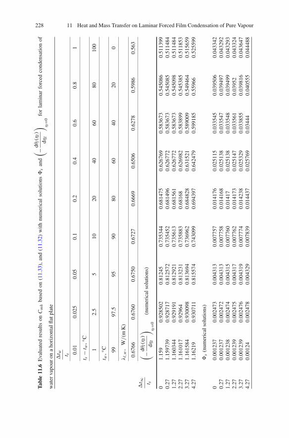
228 11 Heat and Mass Transfer on Laminar Forced Film Condensation of Pure Vapour
Tabl
e11
.6E
valu
ated
resu
ltson
Cm
hba
sed
on(1
1.33
),an
d(1
1.32
)w
ithnu
mer
ical
solu
tions�
san
d
( −dθl(η
l)
dηl
) ηl=
0fo
rla
min
arfo
rced
cond
ensa
tion
of
wat
erva
pour
ona
hori
zont
alfla
tpla
te
�t ∞ t s
�t w t s 0.
010.
025
0.05
0.1
0.2
0.4
0.6
0.8
1
t s−
t w,◦
C
12.
55
1020
4060
8010
0
t w,◦
C 9997
.595
9080
6040
200
λl,w,
W/(m
K)
0.67
660.
6760
0.67
500.
6727
0.66
690.
6506
0.62
780.
5986
0.56
3( −dθ
l(η
l)
dηl
) ηl=
0(n
umer
ical
solu
tions
)
01.
159
0.92
8502
0.81
245
0.73
5344
0.68
1475
0.62
6769
0.58
3673
0.54
5086
0.51
1399
0.27
1.15
9739
0.92
8717
0.81
2572
0.73
5452
0.68
1496
0.62
6772
0.58
3673
0.54
5085
0.51
1484
1.27
1.16
0344
0.92
9191
0.81
2921
0.73
5613
0.68
1561
0.62
6772
0.58
3673
0.54
5098
0.51
1484
2.27
1.16
1017
0.92
964
0.81
3231
0.73
5883
0.68
168
0.62
6982
0.58
3899
0.54
5385
0.51
1853
3.27
1.16
1584
0.93
0098
0.81
3694
0.73
6962
0.68
4828
0.63
1521
0.58
9009
0.54
9464
0.51
5659
4.27
1.16
219
0.93
0711
0.81
5574
0.74
3099
0.69
4397
0.64
2479
0.59
9185
0.55
966
0.52
5599
�s
(num
eric
also
lutio
ns)
00.
0012
370.
0024
730.
0043
130.
0077
570.
0141
760.
0251
150.
0335
450.
0395
060.
0433
420.
270.
0012
370.
0024
720.
0043
130.
0077
580.
0141
680.
0251
380.
0335
470.
0394
970.
0432
921.
270.
0012
380.
0024
740.
0043
150.
0077
600.
0141
70.
0251
380.
0335
480.
0394
990.
0432
932.
270.
0012
390.
0024
750.
0043
170.
0077
620.
0141
730.
0251
470.
0335
610.
0395
20.
0433
243.
270.
0012
390.
0024
760.
0043
190.
0077
740.
0142
380.
0253
290.
0338
550.
0398
160.
0436
474.
270.
0012
40.
0024
780.
0043
290.
0078
390.
0144
370.
0257
690.
0344
40.
0405
550.
0444
88

11.8 Condensate Mass–Energy Transformation Equation 229
Tabl
e11
.6(c
ontin
ued)
Cm
h=( −dθ
l(η
l)
dηl
) ηl=
0
/ �s
(num
eric
alre
sults
)
093
6.94
4237
5.45
5718
8.37
2394.7
975
48.0
724
24.9
5596
17.3
997
13.7
975
11.7
992
0.27
937.
5416
375.
6945
188.
4006
94.7
992
48.1
011
24.9
3325
17.3
986
13.8
006
11.8
147
1.27
937.
273
375.
5824
188.
3942
94.7
955
48.0
989
24.9
3324
17.3
981
13.8
003
11.8
145
2.27
937.
0597
375.
6121
188.
3787
94.8
058
48.0
971
24.9
3267
17.3
981
13.8
002
11.8
145
3.27
937.
5174
375.
6454
018
8.39
8794.7
983
48.0
986
24.9
3272
17.3
979
13.8
001
11.8
143
4.27
937.
2537
5.58
960
188.
3978
094.7
951
48.0
984
24.9
3224
17.3
979
13.8
000
11.8
144
pred
icte
dre
sults
Cm
hw
ithC
mh
=μ
l,sh
fg
λl,w(t
s−
t w)
(μl,
s=
282.
5×
10−6
Kg/(m
s),h
fg=
2257.1
kJ/k
g)
094
2.46
8437
7.29
3518
8.92
4994.7
841
47.8
030
24.5
030
16.9
281
13.3
151
11.3
256
0.27
942.
4684
377.
2935
188.
9249
94.7
841
47.8
030
24.5
0300
16.9
281
13.3
151
11.3
256
1.27
942.
4684
377.
2935
188.
9249
94.7
841
47.8
030
24.5
030
16.9
281
13.3
151
11.3
256
2.27
942.
4684
377.
2935
188.
9249
94.7
841
47.8
030
24.5
030
16.9
280
13.3
151
11.3
256
3.27
942.
4684
377.
2935
188.
9249
94.7
841
47.8
030
24.5
030
16.9
281
13.3
151
11.3
256
4.27
942.
4684
377.
2935
188.
9249
94.7
841
47.8
030
24.5
030
16.9
281
13.3
151
11.3
256
rela
tive
devi
atio
nof
Cm
hpr
edic
ted
byeq
uatio
nsC
mh
=( −dθ
l(η
l)
dηl
) ηl=
0
/ �s
with
num
eric
alre
sults
00.
0059
0.00
489
0.00
293
−0.0
001
−0.0
056
−0.0
18−0.0
27−0.0
350
−0.0
400.
270.
0052
50.
0042
60.
0027
8−0.0
001
−0.0
062
−0.0
173
−0.0
270
−0.0
35−0.0
414
1.27
0.00
554
0.00
455
0.00
282
−0.0
001
−0.0
061
−0.0
173
−0.0
270
−0.0
351
−0.0
414
2.27
0.00
577
0.00
448
0.00
29−0.0
002
−0.0
061
−0.0
172
−0.0
270
−0.0
351
−0.0
414
3.27
0.00
528
0.00
439
0.00
279
−0.0
001
−0.0
061
−0.0
172
−0.0
270
−0.0
351
−0.0
414
4.27
0.00
557
0.00
454
0.00
280
−0.0
001
−0.0
061
−0.0
172
−0.0
270
−0.0
351
−0.0
414
�t ∞ t s
�t w t s
0.01
0.02
50.
050.
10.
20.
40.
60.
81
Not
e:th
epr
esen
tval
ues
ofph
ysic
alpr
oper
tiesλ
l,w
,μl,
s,an
dh
fgar
eco
rres
pond
ing
toth
enu
mer
ical
prog
ram

230 11 Heat and Mass Transfer on Laminar Forced Film Condensation of Pure Vapour
listed in Table 11.6 also. It is seen that the values of mass–energy transformationcoefficient Cmh obtained by the different approaches are well coincident. Then,
it follows that the present calculated results on the key solutions(− dθl (ηl )
dηl
)ηl=0
and �s are reliable, and the condensate mass–heat transfer transformation equation(11.32) with (11.33) is valid.
11.9 Summary
Now it is necessary to summarize in Table 11.7 the governing partial differentialequations, the similarity variables, the similarity governing mathematical models,physical property factor equations, and the condensate heat and mass transfer equa-tions on the two-phase flows laminar forced film condensation of vapour, includingconsideration of a series of interfacial physical matching conditions.
11.10 Remarks
The theoretical equations on condensate heat and mass transfer reported in thischapter based on the new similarity analysis method demonstrate that the walldimensionless temperature gradient and condensate mass flow rate parameter arekey solutions of the governing similarity mathematical model for dominating thecondensate heat and mass transfer results. The laminar forced film condensationof water vapour on a horizontal flat plate is taken as an example, and a system ofnumerical results on the wall dimensionless temperature gradient and condensatemass flow rate parameter is found out rigorously. Meanwhile, the condensate massflow rate parameter depends on the dimensionless condensate film thickness andinterfacial condensate velocity components. Thus, the above theoretical equationson condensate heat and mass transfer become available for reliable prediction ofcondensate heat and mass transfer results for laminar forced film condensation ofwater vapour on a horizontal flat plate.
The variation regulations of the series of physical variables on laminar forcedfilm condensation are clarified. Decreasing the wall subcooled grade will causeincreasing the wall dimensionless temperature gradient; and in the region of lowervapour superheated grade �t∞
ts, the wall dimensionless temperature gradient will
increase at an accelerative pace with decreasing the vapour superheated grade �t∞ts
.Decreasing the wall subcooled grade causes decreasing the condensate liquid filmthickness. In the range of lower wall subcooled grade, the condensate liquid filmthickness will decrease at an accelerative pace with decreasing the condensateliquid film thickness. In addition, increasing the wall subcooled grade will causesincreasing the interfacial liquid dimensionless velocity component Wyl,s(ηlδ) pro-portionally, increasing the interfacial liquid dimensionless velocity componentWxl,s(ηlδ), and increasing the condensate mass flow rate parameter. All these effectsdemonstrate the influence of variable physical properties on condensate heat and
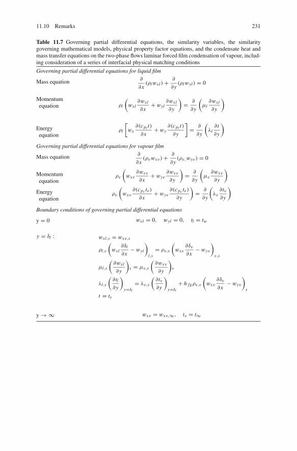
11.10 Remarks 231
Table 11.7 Governing partial differential equations, the similarity variables, the similaritygoverning mathematical models, physical property factor equations, and the condensate heat andmass transfer equations on the two-phase flows laminar forced film condensation of vapour, includ-ing consideration of a series of interfacial physical matching conditions
Governing partial differential equations for liquid film
Mass equation ∂
∂x(ρlwxl )+ ∂
∂y(ρlwyl ) = 0
Momentumequation ρl
(wxl
∂wxl
∂x+ wyl
∂wxl
∂y
)= ∂
∂y
(μl∂wxl
∂y
)
Energyequation
ρl
[wx∂(cpl t)
∂x+ wy
∂(cpl t)
∂y
]= ∂
∂y
(λl∂t
∂y
)
Governing partial differential equations for vapour film
Mass equation ∂
∂x(ρvwxv)+ ∂
∂y(ρv,wyv) = 0
Momentumequation
ρv
(wxv
∂wxv
∂x+ wyv
∂wxv
∂y
)= ∂
∂y
(μv∂wxv
∂y
)
Energyequation
ρv
(wxv
∂(cpv tv)
∂x+ wyv
∂(cpv tv)
∂y
)= ∂
∂y
(λv∂tv∂y
)
Boundary conditions of governing partial differential equations
y = 0 wxl = 0, wyl = 0, tl = tw
y = δl : wxl,s = wxv,s
ρl,s
(wxl
∂δl
∂x− wyl
)
l,s= ρv,s
(wxv
∂δv
∂x− wyv
)
v,s
μl,s
(∂wxl
∂y
)s = μv,s
(∂wxv
∂y
)s
λl,s
(∂tl∂y
)
y=δl= λv,s
(∂tv∂y
)
y=δl+ h fgρv,s
(wxv
∂δv
∂x− wyv
)
s
t = ts
y → ∞ wxv = wxv,∞, tv = t∞

232 11 Heat and Mass Transfer on Laminar Forced Film Condensation of Pure Vapour
Table 11.7 (continued)
Equations of similarity variables
For liquid filmηl = y
x
(1
2Rexl,s
)1/2
Rexl,s = wxv,∞x
νl,s
θl = tl − tstw − ts
wxl = wxv,∞Wxl(ηl)
wyl = wxv,∞(
1
2Rexl,s
)−1/2
Wyl (ηl)
For vapourfilm ηv = y
x
(1
2Rexv,∞
)1/2
Rexv,∞ = wxv,∞x
νv,∞
θv = tv − t∞ts − t∞
wxv = wxv,∞Wxv(ηv)
wyv = wxv,∞(
1
2Rexv,s
)−1/2
Wyv(ηv)
Governing ordinary differential equations for liquid film
Mass equation −ηldWxl(ηl)
dηl+ 2
dWyl (ηl)
dηl+ 1
ρl
dρl
dηl[−ηl Wxl (ηl)+ 2Wyl (ηl )] = 0
Momentumequation
νl,s
νl[−ηl Wxl(ηl)+ 2Wyl (ηl )]dWxl (ηl )
dηl= d2Wxl(ηl )
dη2l
+ 1
μl
dμl
dηl
dWxl(ηl)
dηl
Energyequation Prl
νl,s
νl
⎧⎪⎪⎨⎪⎪⎩
[−ηl · Wxl (ηl)+ 2Wyl (ηl )]dθl(ηl)
dηl
+ [−ηl Wxl (ηl )+ 2Wyl (ηl)] [θl (ηl)+ ts
tw − ts
]1
cpl
dcpl
dηl
⎫⎪⎪⎬⎪⎪⎭
= d2θl(ηl )
dη2l
+ 1
λl
dλl
dηl
dθl(ηl )
dηl

11.10 Remarks 233
Table 11.7 (continued)
Governing ordinary differential equations for vapour film
Mass equation −ηv ∂Wxv(ηv)
∂ηv+ 2
∂Wyv(ηv)
∂ηv− 1
ρv
dρvdηv
[ηvWxv(ηv)+ 2Wyv(ηv)] = 0
Momentumequation
νv,∞νv
[−ηvWxv + 2Wyv]dWxv(ηv)
dηv= d2Wxv(ηv)
dη2v
+ 1
μv
dμvdηv
dWxv(ηv)
dηv
Energyequation Prv
νv,∞νv
⎧⎪⎪⎨⎪⎪⎩
[−Wxv(ηv)ηv + 2Wyv(ηv)] dθv(ηv)
dηv
−[Wxv(ηv)ηv + 2Wyv(ηv)](θv(ηv)+ t∞
ts − t∞
)1
cpv
dcpv
dηv
⎫⎪⎪⎬⎪⎪⎭
= d2θv(ηv)
dη2v
+ 1
λv
dλvdηv
dθv(ηv)
dηv
Boundary conditions of governing ordinary differential equations
ηl = 0 : Wxl(ηl ) = 0, Wyl (ηl ) = 0, θ(ηl ) = 1
ηl = ηlδ Wxv,s(ηv0) = Wxl,s(ηlδ)
Wyv,s(ηv,s) = − ρl,s
ρv,s
(νl,s
νv,s
)1/2 [1
2ηlδWxl,s(ηlδ)− Wyl,s(ηlδ)
]
(dWxv(ηv)
dηv
)
s= μl,s
μv,s
(νv,∞νl,s
)1/2 (dWx (ηl)
dηl
)
s
(dθv(ηv)
dηv
)
s=λl,s
(νv,∞νl,s
)1/2
(tw − ts)
(dθl (ηl )
dηl
)
s+ 2h fgρv,sνv,∞Wyv,s(ηv,0)
λv,s(ts − t∞)θl (ηlδ) = 0 and θv(ηv,0 = 0) = 1
ηv → ∞: Wxv(ηv,∞) = 1, θv(ηv,∞) = 0
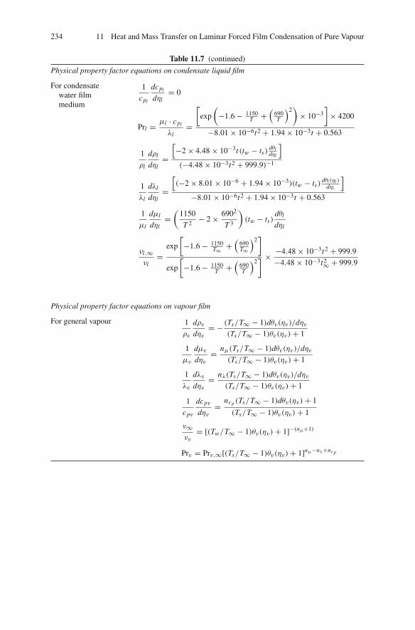
234 11 Heat and Mass Transfer on Laminar Forced Film Condensation of Pure Vapour
Table 11.7 (continued)
Physical property factor equations on condensate liquid film
For condensatewater filmmedium
1
cpl
dcpl
dηl= 0
Prl = μl · cpl
λl=
[exp
(−1.6 − 1150
T +(
690T
)2)
× 10−3]
× 4200
−8.01 × 10⁻⁶t2 + 1.94 × 10⁻³t + 0.563
1
ρl
dρl
dηl=[−2 × 4.48 × 10−3t (tw − ts)
dθldηl
]
(−4.48 × 10⁻³t2 + 999.9)−1
1
λl
dλl
dηl=[(−2 × 8.01 × 10−6 + 1.94 × 10⁻³)(tw − ts)
dθl (ηl )dηl
]
−8.01 × 10⁻⁶t2 + 1.94 × 10⁻³t + 0.563
1
μl
dμl
dηl=(
1150
T 2− 2 × 6902
T 3
)(tw − ts)
dθl
dηl
νl,∞νl
=exp
[−1.6 − 1150
T∞ +(
690T∞
)2]
exp
[−1.6 − 1150
T +(
690T
)2] × −4.48 × 10⁻³t2 + 999.9
−4.48 × 10⁻³t2∞ + 999.9
Physical property factor equations on vapour film
For general vapour 1
ρv
dρvdηv
= − (Ts/T∞ − 1)dθv(ηv)/dηv(Ts/T∞ − 1)θv(ηv)+ 1
1
μv
dμvdηv
= nμ(Ts/T∞ − 1)dθv(ηv)/dηv(Ts/T∞ − 1)θv(ηv)+ 1
1
λv
dλvdηv
= nλ(Ts/T∞ − 1)dθv(ηv)/dηv(Ts/T∞ − 1)θv(ηv)+ 1
1
cpv
dcpv
dηv= ncp (Ts/T∞ − 1)dθv(ηv)+ 1
(Ts/T∞ − 1)θv(ηv)+ 1
ν∞νv
= [(Tw/T∞ − 1)θv(ηv)+ 1]−(nμ+1)
Prv = Prv,∞[(Ts/T∞ − 1)θv(ηv)+ 1]nμ−nλ+ncp

11.10 Remarks 235
Table 11.7 (continued)
Condensate heat transfer
Wall dimensionlesstemperaturegradient
−(
dθl (ηl )
dηl
)
ηl=0
For laminar forced film condensation of water vapour on a horizon-tal plate
for 0 ≤ �t∞ts
≤ 4.27
−(
dθl (ηl )
dηl
)
ηl=0=
0.7421�tw
ts+ 0.3124
(�tw
ts
)0.28(0.01 ≤ �tw
ts≤ 0.1)
−(
dθl (ηl)
dηl
)
ηl =0= 0.1466
(�tw
ts
)2 − 0.3974
(�tw
ts
)+ 0.7652
(0.1 ≤ �tw
ts≤ 1
)
Local values onheat transfer
Nuxl,w = αx,wx
λl,w
qx,w = λl,w(tw − ts)
(1
2Rexl,s
)1/2
x−1(
−dθl(ηl)
dηl
)
ηl =0
αx,w = λl,w
(1
2Rexl,s
)1/2
x−1(
−dθl(ηl)
dηl
)
ηl =0
Nuxl,w =(
1
2Rexl,s
)1/2 (−dθl(ηl )
dηl
)
ηl =0
Average values onheat transfer
Nuxl,w = αx,wx
λl,w
Qx,w = √2x−1λl,w(tw − ts)(Rexl,s)
1/2(
−dθl(ηl)
dηl
)
ηl =0
αx,w = √2λl,wRexl,s
1/2x−1(
−dθl(ηl )
dηl
)
ηl =0
Nuxl,w = √2(Rexl,s)
1/2(
−dθl (ηl)
dηl
)
ηl=0
Total value on heattransfer
Qx,w = √2bλl,w(tw − ts)(Rexl,s)
1/2(
−dθl(ηl )
dηl
)
ηl =0

236 11 Heat and Mass Transfer on Laminar Forced Film Condensation of Pure Vapour
Table 11.7 (continued)
Condensate mass flow rate
Mass flow rateParameter �s
For laminar forced film condensation of water
vapour on a horizontal plate for 0 ≤ �t∞ts
≤ 4.27
�s = 0.0719
(�tw
ts
)+ 0.00057
(0.01 ≤ �tw
ts≤ 0.1
)
�s = −0.0301
(�tw
ts
)2
+ 0.0725
(�tw
ts
)+ 0.0008
(0.1 ≤ �tw
ts≤ 1
)
Mass flow rate GxGx = √
2bμl,sRexl,s1/2�s
Condensate mass–energy transformation equation
(−dθl (ηl)
dηl
)
ηl =0= Cmh�s ,
Condensate mass–energy transformation coefficient
Cmh = μl,sh fg
λl,w(ts − tw)
mass transfer. Compared with the effect of the wall subcooled grade on these keyphysical variables, the effect of the vapour superheated grade is very slight in thebroad range of the vapour superheated grade, and can be ignored for practical pre-diction of these key physical variables without any obvious deviation to the predic-tion results.
On the basis of the above analysis, by using the curve-fitting approach, the systemof these rigorous key numerical solutions for laminar forced film condensation ofwater vapour on a horizontal flat plate is formulated with variation of the wall sub-cooled grade, and these formulated equations are coincident very well to the relatedkey solutions. With the formulated equations on the wall dimensionless temperaturegradient and condensate mass flow rate parameter, the above theoretical equationson heat and mass transfer become available for simple and reliable prediction ofcondensate heat and mass transfer results.
The condensate mass–energy transformation equation provided in this chapterdemonstrates the internal relation between the condensate heat and mass transfer,and is the general equation suitable for all laminar forced film condensation. Thecondensate mass–energy transformation coefficient is proportional to the physicalfactor
h fgcpl,s (ts−tw)
, interfacial liquid Prandtl number Prl,s , and the liquid thermal
conductivity ratio λl,sλl,w
in the broad range of the vapour superheated grade.
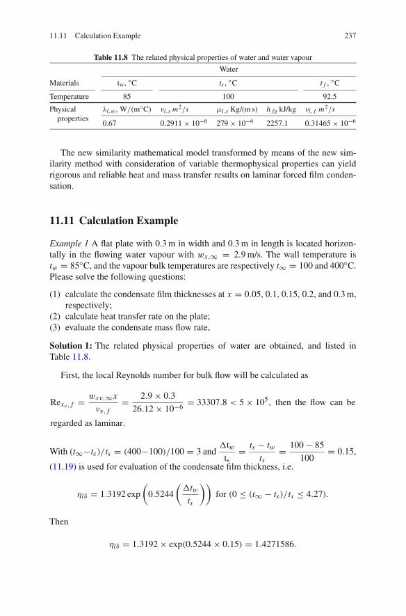
11.11 Calculation Example 237
Table 11.8 The related physical properties of water and water vapour
Water
Materials tw, ◦C ts , ◦C t f , ◦C
Temperature 85 100 92.5
Physicalproperties
λl,w , W/(m◦C) νl,s m2/s μl,s Kg/(m s) h fg kJ/kg νl, f m2/s
0.67 0.2911 × 10⁻⁶ 279 × 10−6 2257.1 0.31465 × 10⁻⁶
The new similarity mathematical model transformed by means of the new sim-ilarity method with consideration of variable thermophysical properties can yieldrigorous and reliable heat and mass transfer results on laminar forced film conden-sation.
11.11 Calculation Example
Example 1 A flat plate with 0.3 m in width and 0.3 m in length is located horizon-tally in the flowing water vapour with wx,∞ = 2.9 m/s. The wall temperature istw = 85◦C, and the vapour bulk temperatures are respectively t∞ = 100 and 400◦C.Please solve the following questions:
(1) calculate the condensate film thicknesses at x = 0.05, 0.1, 0.15, 0.2, and 0.3 m,respectively;
(2) calculate heat transfer rate on the plate;(3) evaluate the condensate mass flow rate,
Solution 1: The related physical properties of water are obtained, and listed inTable 11.8.
First, the local Reynolds number for bulk flow will be calculated as
Rexv, f = wxv,∞x
νv, f= 2.9 × 0.3
26.12 × 10−6 = 33307.8 < 5 × 10⁵, then the flow can be
regarded as laminar.
With (t∞−ts)/ts = (400−100)/100 = 3 and�tw
ts= ts − tw
ts= 100 − 85
100= 0.15,
(11.19) is used for evaluation of the condensate film thickness, i.e.
ηlδ = 1.3192 exp
(0.5244
(�tw
ts
))for (0 ≤ (t∞ − ts)/ts ≤ 4.27).
Then
ηlδ = 1.3192 × exp(0.5244 × 0.15) = 1.4271586.
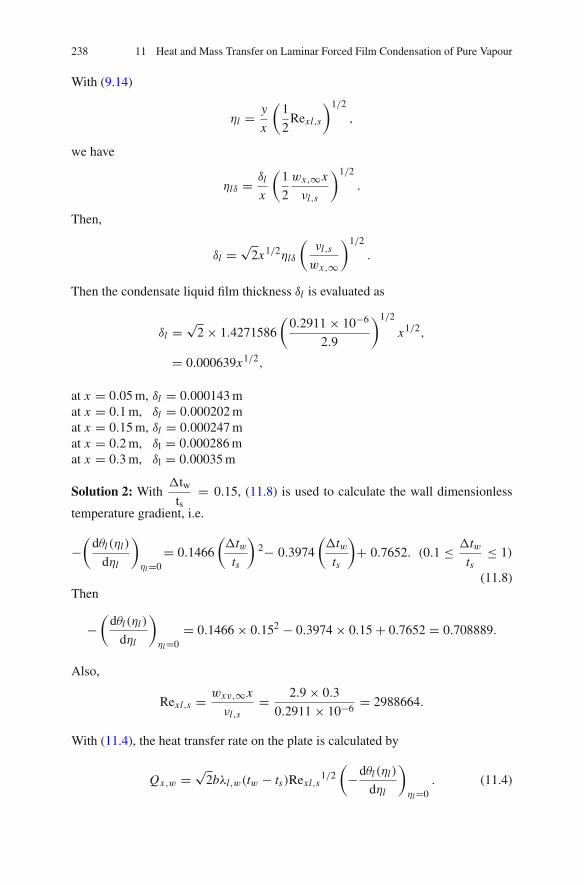
238 11 Heat and Mass Transfer on Laminar Forced Film Condensation of Pure Vapour
With (9.14)
ηl = y
x
(1
2Rexl,s
)1/2
,
we have
ηlδ = δl
x
(1
2
wx,∞x
νl,s
)1/2
.
Then,
δl = √2x1/2ηlδ
(νl,s
wx,∞
)1/2
.
Then the condensate liquid film thickness δl is evaluated as
δl = √2 × 1.4271586
(0.2911 × 10⁻⁶
2.9
)1/2
x1/2,
= 0.000639x1/2,
at x = 0.05 m, δl = 0.000143 mat x = 0.1 m, δl = 0.000202 mat x = 0.15 m, δl = 0.000247 mat x = 0.2 m, δl = 0.000286 mat x = 0.3 m, δl = 0.00035 m
Solution 2: With�tw
ts= 0.15, (11.8) is used to calculate the wall dimensionless
temperature gradient, i.e.
−(
dθl(ηl)
dηl
)
ηl=0= 0.1466
(�tw
ts
)2− 0.3974
(�tw
ts
)+ 0.7652. (0.1 ≤ �tw
ts≤ 1)
(11.8)Then
−(
dθl(ηl)
dηl
)
ηl=0= 0.1466 × 0.152 − 0.3974 × 0.15 + 0.7652 = 0.708889.
Also,
Rexl,s = wxv,∞x
νl,s= 2.9 × 0.3
0.2911 × 10−6 = 2988664.
With (11.4), the heat transfer rate on the plate is calculated by
Qx,w = √2bλl,w(tw − ts)Rexl,s
1/2(
−dθl(ηl)
dηl
)
ηl=0. (11.4)

Exercises 239
Then the plate condensate heat transfer rate is
Qx,w = √2 × 0.3 × 0.67 × (85 − 100)× 29886641/2 × 0.708889 = −5225.4 W.
The negative result of the evaluated total heat transfer rate show that the heat fluxdirection is from the vapour bulk to the plate wall.
Solution 3: With�tw
ts= 0.15, (11.25) is used to calculate the condensate mass
flow rate parameter for laminar forced film flows of water vapour on a horizontalflat plate, i.e.
�s = −0.0301
(�tw
ts
)2
+ 0.0725
(�tw
ts
)+ 0.0008
(0.1 ≤ �tw
ts≤ 1
)
(11.25)Then
�s = −0.0301 × 0.152 + 0.0725 × 0.15 + 0.0008 = 0.010998.
Equation (11.17) can be used for evaluation of condensate heat transfer rate on theplate, i.e.
Gx = √2bμl,s Rexl,s
1/2�s . (11.17)
Therefore,
Gx = √2×0.3×279×10−6×29886641/2×0.010998 = 0.002251 kg/s = 8.1 kg/h.
Exercises
1. Point out the suitable scope of the condensate mass-energy transformation equa-tion reported in this chapter.
2. Continued to Example 1, suppose the wall temperature tw = 65˚C, but keep allother conditions. Please solve the following:
(1) calculate the condensate film thicknesses at x = 0.05, 0.1, 0.15, 0.2, and0.3 m;
(2) calculate heat transfer rate on the plate;(3) evaluate the condensate mass flow rate.
3. Suppose that the wall dimensionless temperature gradient is 0.68, and keep allother related conditions of Example 1. Please use two different approaches toevaluate the total condensate mass flow rate.

Chapter 12Complete Similarity Mathematical Modelson Laminar Forced Film Condensationof Vapour–Gas Mixture
Abstract The complete similarity mathematical model based on the new similarityanalysis method is developed for laminar forced film condensation from vapour–gasmixture. The governing similarity mathematical models for the liquid and vapourfilm flows are coupled by the seven interfacial matching conditions respectively forthe two-dimensional velocity component balances, shear force balance, mass flowrate balance, temperature balance, heat transfer balance, concentration condition,as well as the balance between the condensate liquid mass flow and vapour massdiffusion. The work of this chapter is the successful application of the present newsimilarity analysis method to the extensive investigation of the laminar forced filmcondensation of vapour–gas mixture, and the developed mathematical model is acomplete dimensionless similarity model. In the complete similarity model both forliquid and vapour–gas mixture films, the concentration and temperature-dependentphysical properties, such as variable density, thermal conductivity, viscosity, andspecific heat, are taken into account. These variable physical properties exist in thetransformed governing similarity mathematical model as the related dimensionlessphysical factors. The investigation of this chapter proves that the present new sim-ilarity analysis method developed in this book is a better alternative to the tradi-tional Falkner-Skan type transformation for extensive investigation of laminar filmcondensation.
12.1 Introduction
Film condensation phenomenon exists in many industrial departments, and film con-densation from vapour in presence of noncondensable gas plays an important rolein the design of heat exchangers, and in the heat transfer process of the chemicaland power industry including nuclear power plants. Then numerous theoretical andexperimental studies have been done for its successive investigations, such as thosein [1–23], and some detailed reviews of condensation heat and mass transfer canbe found in [24–28]. These studies demonstrate that the bulk concentration of thenoncondensable gas could have a decisive effect on the condensate heat transferrate, and their results indicated greater reductions in heat transfer. This is becauseof the fact that the presence of non-condensable gas lowers the partial pressure of
D.Y. Shang, Theory of Heat Transfer with Forced Convection Film Flows,Heat and Mass Transfer, DOI 10.1007/978-3-642-12581-2_12,C© Springer-Verlag Berlin Heidelberg 2011
241
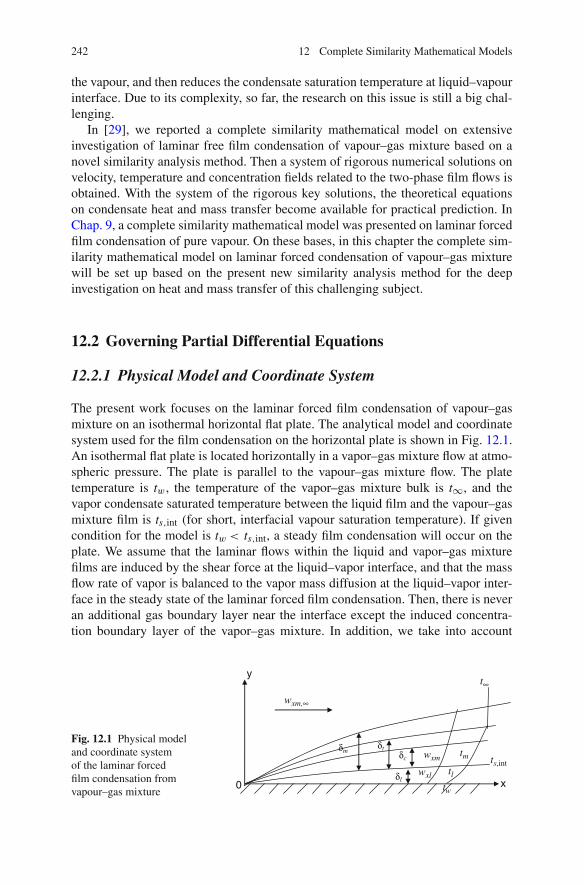
242 12 Complete Similarity Mathematical Models
the vapour, and then reduces the condensate saturation temperature at liquid–vapourinterface. Due to its complexity, so far, the research on this issue is still a big chal-lenging.
In [29], we reported a complete similarity mathematical model on extensiveinvestigation of laminar free film condensation of vapour–gas mixture based on anovel similarity analysis method. Then a system of rigorous numerical solutions onvelocity, temperature and concentration fields related to the two-phase film flows isobtained. With the system of the rigorous key solutions, the theoretical equationson condensate heat and mass transfer become available for practical prediction. InChap. 9, a complete similarity mathematical model was presented on laminar forcedfilm condensation of pure vapour. On these bases, in this chapter the complete sim-ilarity mathematical model on laminar forced condensation of vapour–gas mixturewill be set up based on the present new similarity analysis method for the deepinvestigation on heat and mass transfer of this challenging subject.
12.2 Governing Partial Differential Equations
12.2.1 Physical Model and Coordinate System
The present work focuses on the laminar forced film condensation of vapour–gasmixture on an isothermal horizontal flat plate. The analytical model and coordinatesystem used for the film condensation on the horizontal plate is shown in Fig. 12.1.An isothermal flat plate is located horizontally in a vapor–gas mixture flow at atmo-spheric pressure. The plate is parallel to the vapour–gas mixture flow. The platetemperature is tw, the temperature of the vapor–gas mixture bulk is t∞, and thevapor condensate saturated temperature between the liquid film and the vapour–gasmixture film is ts,int (for short, interfacial vapour saturation temperature). If givencondition for the model is tw < ts,int, a steady film condensation will occur on theplate. We assume that the laminar flows within the liquid and vapor–gas mixturefilms are induced by the shear force at the liquid–vapor interface, and that the massflow rate of vapor is balanced to the vapor mass diffusion at the liquid–vapor inter-face in the steady state of the laminar forced film condensation. Then, there is neveran additional gas boundary layer near the interface except the induced concentra-tion boundary layer of the vapor–gas mixture. In addition, we take into account
Fig. 12.1 Physical modeland coordinate systemof the laminar forcedfilm condensation fromvapour–gas mixture
y
x0
wxm,∞
t∞
ts,intwxl tl
tmwxm
tw
δc
δtδm
δl

12.2 Governing Partial Differential Equations 243
the temperature-dependent physical properties of the condensate liquid film and thetemperature and concentration-dependent physical properties of the induced vapor–gas mixture film. Then the steady laminar governing equations for mass, momen-tum, energy and concentration conservations in the two-phase boundary layer are asfollows.
12.2.2 Governing Partial Differential Equations
12.2.2.1 For Liquid Film
The governing partial differential equations for condensate liquid film are
∂
∂x(ρlwxl)+ ∂
∂y(ρlwyl) = 0, (12.1)
ρl
(wxl
∂wxl
∂x+ wyl
∂wxl
∂y
)= ∂
∂y
(μl∂wxl
∂y
), (12.2)
ρv
[wxl
∂(cpv tl)
∂x+ wyl
∂(cpv tl)
∂y
]= ∂
∂y
(λl∂tl∂y
), (12.3)
where (12.1), (12.2), and (12.3) are continuity, momentum, and energy conservationequations, respectively. Here the liquid temperature-dependent physical properties,such as density ρl , absolute viscosity μl , thermal conductivity λl , and specific heatcpl are considered. While, wxl and wyl are liquid film velocity components respec-tively in x and y coordinates.
12.2.2.2 For Vapour–Gas Mixture Film
The governing partial differential equations for vapour film are,
∂
∂x(ρmwxm)+ ∂
∂y(ρmwym) = 0 (12.4)
ρm
(wxm
∂wxm
∂x+ wym
∂wxm
∂y
)= ∂
∂y
(μm
∂wxm
∂y
), (12.5)
ρm
[wxm
∂(cpm tm)
∂x+ wym
∂(cpm tm)
∂y
]= ∂
∂y
(λm∂tm∂y
)
+ ∂
∂y
[ρm Dv(cpv − cpa )
∂Cmv
∂ytm
],
(12.6)
∂(wxmρmCmv)
∂x+ ∂(wymρmCmv)
∂y= ∂
∂y
(Dvρm
∂Cmv
∂y
), (12.7)
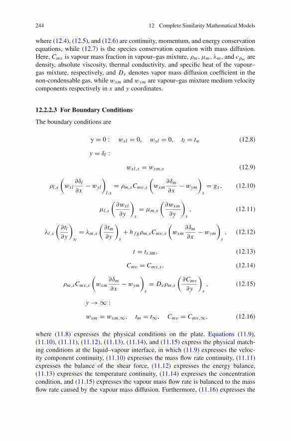
244 12 Complete Similarity Mathematical Models
where (12.4), (12.5), and (12.6) are continuity, momentum, and energy conservationequations, while (12.7) is the species conservation equation with mass diffusion.Here, Cmv is vapour mass fraction in vapour–gas mixture, ρm , μm , λm , and cpm aredensity, absolute viscosity, thermal conductivity, and specific heat of the vapour–gas mixture, respectively, and Dv denotes vapor mass diffusion coefficient in thenon-condensable gas, while wxm and wym are vapour–gas mixture medium velocitycomponents respectively in x and y coordinates.
12.2.2.3 For Boundary Conditions
The boundary conditions are
y = 0 : wxl = 0, wyl = 0, tl = tw (12.8)
y = δl :wxl,s = wxm,s (12.9)
ρl,s
(wxl
∂δl
∂x− wyl
)
l,s= ρm,sCmv,s
(wxm
∂δm
∂x− wym
)
s= gx , (12.10)
μl,s
(∂wxl
∂y
)
s= μm,s
(∂wxm
∂y
)
s, (12.11)
λl,s
(∂tl∂y
)
sl
= λm,s
(∂tm∂y
)
s+ h f gρm,sCmv,s
(wxm
∂δm
∂x− wym
)
s, (12.12)
t = ts,int, (12.13)
Cmv = Cmv,s, (12.14)
ρm,sCmv,s
(wxm
∂δm
∂x− wym
)
s= Dvρm,s
(∂Cmv
∂y
)
s, (12.15)
y → ∞ :wxm = wxm,∞, tm = t∞, Cmv = Cmv,∞, (12.16)
where (11.8) expresses the physical conditions on the plate. Equations (11.9),(11.10), (11.11), (11.12), (11.13), (11.14), and (11.15) express the physical match-ing conditions at the liquid–vapour interface, in which (11.9) expresses the veloc-ity component continuity, (11.10) expresses the mass flow rate continuity, (11.11)expresses the balance of the shear force, (11.12) expresses the energy balance,(11.13) expresses the temperature continuity, (11.14) expresses the concentrationcondition, and (11.15) expresses the vapour mass flow rate is balanced to the massflow rate caused by the vapour mass diffusion. Furthermore, (11.16) expresses the
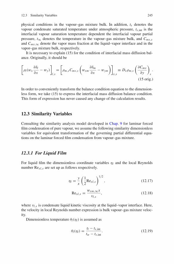
12.3 Similarity Variables 245
physical conditions in the vapour–gas mixture bulk. In addition, ts denotes thevapour condensate saturated temperature under atmospheric pressure, ts,int is theinterfacial vapour saturation temperature dependent the interfacial vapour partialpressure, t∞ denotes the temperature in the vapour–gas mixture bulk, and Cmv,sand Cmv,∞ denote the vapor mass fraction at the liquid–vapor interface and in thevapor–gas mixture bulk, respectively.
It is necessary to explain (15) for the condition of interfacial mass diffusion bal-ance. Originally, it should be
[ρl(wx
∂δl
∂x− wy)
]
l,s=[ρm,sCmv,s
(wxm
∂δm
∂x− wym
)]
v,s≡ Dvρm,s
(∂Cmv
∂y
)
s.
(15 orig.)
In order to conveniently transform the balance condition equation to the dimension-less form, we take (15) to express the interfacial mass diffusion balance condition.This form of expression has never caused any change of the calculation results.
12.3 Similarity Variables
Consulting the similarity analysis model developed in Chap. 9 for laminar forcedfilm condensation of pure vapour, we assume the following similarity dimensionlessvariables for equivalent transformation of the governing partial differential equa-tions on the laminar forced film condensation from vapour–gas mixture.
12.3.1 For Liquid Film
For liquid film the dimensionless coordinate variables ηl and the local Reynoldsnumber Rexl,s are set up as follows respectively.
ηl = y
x
(1
2Rexl,s
)1/2
, (12.17)
Rexl,s = wxm,∞x
νl,s, (12.18)
where νl,s is condensate liquid kinetic viscosity at the liquid–vapor interface. Here,the velocity in local Reynolds number expression is bulk vapour–gas mixture veloc-ity.
Dimensionless temperature θl(ηl) is assumed as
θl(ηl) = tl − ts,int
tw − ts,int. (12.19)

246 12 Complete Similarity Mathematical Models
While the dimensionless velocity components Wxl(ηl) and Wyl(ηl) in x - and y -directions are given as, respectively,
wxl = wxm,∞Wxl(ηl), (12.20)
wyl = wxm,∞(
1
2Rexl,s
)−1/2
Wyl(ηl). (12.21)
It is noted that here the velocity in equations of the local Reynolds number Rexl,s
and the dimensionless velocity components Wxl (ηl) and Wyl(ηl) is the vapour–gasmixture bulk velocity wxm,∞.
12.3.2 For Vapor–Gas Mixture Film
For vapor–gas mixture film, the similarity dimensionless coordinate variable ηm andthe local Reynolds number Rexm,∞ are assumed as respectively
ηm = y
x
(1
2Rexm,∞
)1/2
, (12.22)
Rexm,∞ = wxm,∞x
νm,∞. (12.23)
The dimensionless temperature θm is defined as
θm(ηm) = tm − t∞ts,int − t∞
, (12.24)
where ts,int is the interfacial vapour saturation temperature, dependent on the inter-facial vapour mass fraction Cmv,s .
The similarity dimensionless velocity components Wxm(ηm) and Wym(ηm) areassumed as respectively in x and y directions
wxm = wxm,∞Wxm(ηm), (12.25)
wym = wxm,∞(
1
2Rexm,∞
)−1/2
Wym(ηm). (12.26)
It is noted that here the velocity in equations of the local Reynolds number Rexm,∞and the dimensionless velocity components Wxm(ηm) and Wym(ηm) is the vapour–gas mixture bulk velocity wxm,∞.
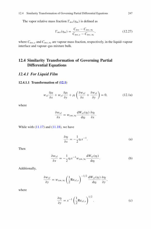
12.4 Similarity Transformation of Governing Partial Differential Equations 247
The vapor relative mass fraction �mv(ηm) is defined as
�mv(ηm) = Cmv − Cmv,∞Cmv,s − Cmv,∞
, (12.27)
where Cmv,s and Cmv,∞ are vapour mass fraction, respectively, in the liquid–vapourinterface and vapour–gas mixture bulk.
12.4 Similarity Transformation of Governing PartialDifferential Equations
12.4.1 For Liquid Film
12.4.1.1 Transformation of (12.1)
wxl∂ρl
∂x+ wyl
∂ρl
∂y+ ρl
(∂wxl
∂x+ ∂wyl
∂y
)= 0, (12.1a)
where
∂wxl
∂x= wxm,∞
dWxl(ηl)
dηl
∂ηl
∂x.
While with (11.17) and (11.18), we have
∂ηl
∂x= −1
2ηl x
−1. (a)
Then
∂wxl
∂x= −1
2ηl x
−1wxm,∞dWxl(ηl)
dηl. (b)
Additionally,
∂wyl
∂y= wxm,∞
(1
2Rexl,s
)−1/2 dWyl(ηl)
dηl
∂ηl
∂y,
where
∂ηl
∂y= x−1
(1
2Rexl,s
)1/2
. (c)

248 12 Complete Similarity Mathematical Models
Then
∂wyl
∂y= wxm,∞
dWyl(ηl)
dηlx−1. (d)
Furthermore,
∂ρl
∂x= dρl
dηl
∂ηl
∂x= −1
2
dρl
dηlηl x
−1, (e)
∂ρl
∂y= dρl
dηl
∂ηl
∂y= dρl
dηlx−1(
1
2Rexl,s
)1/2
. (f)
With (11.20), (11.21), (b), (d) to (f), (12.1a) is changed to
ρl
[−1
2ηl x
−1wxv,∞dWxl (ηl)
dηl+ wxv,∞
dWyl(ηl)
dηlx−1]
− 1
2
dρl
dηlηl x
−1wxv,∞Wxl(ηl)+ dρl
dηlx−1(
1
2Rexl,s
)1/2
wxv,∞(
1
2Rexl,s
)−1/2
Wyl(ηl) = 0
The above equation is divided by x−1wxm,∞ and becomes
ρl
[−1
2ηl
dWxl(ηl)
dηl+ dWyl(ηl)
dηl
]− 1
2
dρl
dηlηl Wxl(ηl)+ dρl
dηlWyl(ηl).
The above equation is further divided byρl
2and becomes
− ηldWxl(ηl)
dηl+ 2
dWyl(ηl)
dηl+ 1
ρl
dρl
dηl[−ηl Wxl(ηl)+ 2Wyl(ηl)] = 0. (12.28)
12.4.1.2 Transformation of (12.2)
Equation (12.2) is changed to
ρl
(wxl
∂wxl
∂x+ wyl
∂wxl
∂y
)= μl
∂2wxv
∂y2 + ∂μl
∂y
∂wxv
∂y, (12.2a)
where
∂wxl
∂y= wxm,∞
dWxl(ηl)
dηl
∂ηl
∂y.

12.4 Similarity Transformation of Governing Partial Differential Equations 249
With (12.d), the above equation is changed to
∂wxl
∂y= wxm,∞
dWxl (ηl)
dηlx−1(
1
2Rexl,s
)1/2
, (g)
or
∂2wxl
∂y2=wxm,∞
d2Wxl(ηl)
dη2l
x−1(
1
2Rexl,s
)1/2∂ηl
∂y
=wxm,∞d2Wxl(ηl)
dη2l
x−2(
1
2Rexl,s
).
(h)
Similar to (f), we have
∂μl
∂y= dμl
dηlx−1(
1
2Rexl,s
)1/2
. (i)
With (12.20), (12.21), (b), (g) to (i), (12.2a) is changed to
ρl
⎡⎢⎢⎢⎣
−wxm,∞Wxl(ηl)1
2ηl x−1wxm,∞
dWxl(ηl)
dηl
+wxm,∞(
1
2Rexl,s
)−1/2
Wyl(ηl) · wxm,∞dWxl (ηl)
dηlx−1(
1
2Rexl,s
)1/2
⎤⎥⎥⎥⎦
= μlwxm,∞d2Wxl(ηl)
dη2l
x−2(
1
2Rexl,s
)
+ dμl
dηlx−1(
1
2Rexl,s
)1/2
wxm,∞dWxl(ηl)
dηlx−1(
1
2Rexl,s
)1/2
.
With the definition of Rexl,s , the above equation becomes
ρl
[−wxm,∞Wxl (ηl)
1
2ηl x−1wxm,∞
dWxl (ηl)
dηl+ wxm,∞(Wyl (ηl ) · wxm,∞
dWxl (ηl )
dηlx−1]
= μlwxm,∞d2Wxl (ηl )
dη2l
x−2(
1
2
wxm,∞x
νl,s
)+ dμl
dηlx−1(
1
2
wxm,∞x
νl,s
)wxm,∞
dWxl (ηl)
dηlx−1.

250 12 Complete Similarity Mathematical Models
The above equation is divided by1
2x−1 · w2
xm,∞, and becomes
ρl
[−Wxl(ηl)ηl
dWxl(ηl)
dηl+ 2(Wyl(ηl) · dWxl(ηl)
dηl
]=μl
d2Wxl(ηl)
dη2l
(1
νl,s
)
+ dμl
dηl
(1
νl,s
)dWxl(ηl)
dηl.
The above equation is divided byμl
νl,s, and becomes
νl,s
νl[−ηl Wxl(ηl)+2(Wyl(ηl)]dWxl(ηl)
dηl= d2Wxl(ηl)
dη2l
+ 1
μl
dμl
dηl
dWxl (ηl)
dηl. (12.29)
12.4.1.3 Transformation of (12.3)
Equation (12.3) is changed to
ρl
(wxlcpl
∂tl∂x
+ wxl tl∂cpl
∂x+ wylcpl
∂tl∂y
+ wyl tl∂cpl
∂y
)= λl
∂2tl∂y2
+ ∂λl
∂y
∂tl∂y,
(12.3a)where
∂tl∂x
= dtldηl
∂ηl
∂x.
While
dtldηl
= (tw − ts,int)dθl(ηl)
dηl. (j)
With (b) and (k), we have
∂tl∂x
= −1
2ηl x
−1(tw − ts,int)dθl(ηl)
dηl. (k)
Additionally,
∂tl∂y
= dtldηl
∂ηl
∂y.
With (d) and (k), we have
∂tl∂y
= x−1(
1
2Rexl,s
)1/2
(tw − ts,int)dθl(ηl)
dηl, (l)
12.4 Similarity Transformation of Governing Partial Differential Equations 251
or
∂2tl∂y2 = x−2
(1
2Rexl,s
)(tw − ts,int)
d2θl(ηl)
d2ηl. (m)
Similar to (f), we have
∂λl
∂y= dλl
dηlx−1(
1
2Rexl,s
)1/2
, (n)
∂cpl
∂y= dcpl
dηlx−1(
1
2Rexl,s
)1/2
. (o)
Similar to (e),
∂cpl
∂x= −1
2
dcpl
dηlηl x
−1. (p)
With (12.20), (12.21), (k) to (p), (12.3a) is changed to
ρl
⎡⎢⎢⎢⎢⎢⎢⎢⎢⎢⎢⎣
wxm,∞Wxl(ηl )cpl
(−1
2ηl x−1(tw − ts,int)
dθl (ηl)
dηl
)+ wxm,∞Wxl(ηl )tl
(−1
2ηl x−1 dcpl
dηl
)
+wxm,∞(
1
2Rexl,∞
)−1/2
Wyl (ηl )cpl x−1(
1
2Rexl,s
)1/2
(tw − ts,int)dθl(ηl)
dηl
+wxm,∞(
1
2Rexl,s
)−1/2
Wyl (ηl)tldcpl
dηlx−1(
1
2Rexl,∞
)1/2
⎤⎥⎥⎥⎥⎥⎥⎥⎥⎥⎥⎦
= λl x−2(
1
2Rexl,s
)(tw − ts,int)
d2θl (ηl )
dη2l
+ ∂λl
∂ηlx−1(
1
2Rexl,s)
)1/2
x−1(
1
2Rexl,s
)1/2
(tw − ts,int)dθl (ηl )
dηl,
or
ρl
⎡⎢⎢⎢⎣
wxm,∞Wxl(ηl )cpl
(−1
2ηl x−1(tw − ts,int)
dθl (ηl)
dηl
)+ wxm,∞Wxl(ηl )tl
(−1
2ηl x−1 dcpl
dηl
)
+wxm,∞Wyl (ηl )cpl x−1(tw − ts,int)dθl (ηl )
dηl+ wxm,∞Wyl (ηl)tl
dcpl
dηlx−1
⎤⎥⎥⎥⎦
= λl x−2(
1
2Rexl,s
)(tw − ts,int)
d2θl (ηl )
dη2l
+ ∂λl
∂ηlx−1(
1
2Rexl,s
)x−1(tw − ts,int)
dθl(ηl )
dηl.

252 12 Complete Similarity Mathematical Models
With definition of Rexl,s , the above equation is changed to
ρl
⎡⎢⎢⎢⎣
wxm,∞Wxl(ηl )cpl
(−1
2ηl x−1(tw − ts,int)
dθl (ηl)
dηl
)+ wxm,∞Wxl(ηl )tl
(−1
2ηl x−1 dcpl
dηl
)
+wxm,∞Wyl (ηl )cpl x−1(tw − ts,int)dθl (ηl )
dηl+ wxm,∞Wyl (ηl)tl
dcpl
dηlx−1
⎤⎥⎥⎥⎦
= λl x−2(
1
2
wxm,∞x
νl,s
)(tw − ts,int)
d2θl(ηl)
dη2l
+ ∂λl
∂ηlx−1(
1
2
wxm,∞x
νl,s
)x−1(tw − ts,int)
dθl(ηl )
dηl.
The above equation is divided by x−1wxm,∞(tw − ts,int), and becomes
ρl cpl
⎡⎢⎢⎢⎣
Wxl(ηl)
(−1
2ηl
dθl(ηl)
dηl
)+ Wxl(ηl)
tltw − ts,int
(−1
2ηl
1
cpl
dcpl
dηl
)
+Wyl(ηl)dθl(ηl)
dηl+ Wyl(ηl)
tltw − ts,int
1
cpl
dcpl
dηl
⎤⎥⎥⎥⎦
= λl
(1
2
1
νl,s
)d2θl(ηl)
dη2l
+ ∂λl
∂ηl
(1
2
1
νl,s
)dθl(ηl)
dηl.
The above equation is divided byλl
2νl,s, and further simplified to
νl,s
λlρl cpl
⎡⎢⎢⎢⎣
Wxl(ηl)
(−ηl
dθl(ηl)
dηl
)+ Wxl (ηl)
tltw − ts,int
(−ηl
1
cpl
dcpl
dηl
)
+ 2Wyl(ηl)dθl(ηl)
dηl+ 2Wyl(ηl)
tltw − ts,int
1
cpl
dcpl
dηl
⎤⎥⎥⎥⎦
= d2θl(ηl)
dη2l
+ 1
λl
∂λl
∂ηl
dθl(ηl)
dηl,
i.e.
Prlνl,s
νl
([−ηl Wxl(ηl)+ 2Wyl(ηl)]dθl(ηl)
dηl
+[−ηl Wxl(ηl)+ 2Wyl(ηl)] tltw − ts,int
1
cpl
dcpl
dηl
)= d2θl(ηl)
dη2l
+ 1
λl
∂λl
∂ηl
dθl(ηl)
dηl.
Withtl
tw − ts,int= θl(ηl)+ ts,int
tw − ts,int, the above equation is changed to

12.4 Similarity Transformation of Governing Partial Differential Equations 253
Prlνl,s
νl
⎛⎜⎜⎜⎝
[−ηl Wxl (ηl)+ 2Wyl(ηl)]dθl(ηl)
dηl
+[−ηl Wxl(ηl)+ 2Wyl(ηl)](θl(ηl)+ ts,int
tw − ts,int
)1
cpl
dcpl
dηl
⎞⎟⎟⎟⎠
= d2θl(ηl)
dη2l
+ 1
λl
∂λl
∂ηl
dθl(ηl)
dηl.
(12.30)
In fact, the derived (12.30) is same as (9.26) although some differences exist in theexpressions of the related similarities variables.
12.4.2 For Vapour–Gas Mixture Film
With the similar derivation to that in Sect. 12.4.1, we have the following equations:
∂ηm
∂x= −1
2ηm x−1, (aa)
∂wxm
∂x= −1
2ηm x−1wxm,∞
dWxm(ηm)
dηm, (bb)
∂ηm
∂y= x−1
(1
2Rexm,∞
)1/2
, (cc)
∂wym
∂y= wxm,∞
dWym(ηm)
dηmx−1, (dd)
∂ρm
∂x= −1
2
dρm
dηmηm x−1, (ee)
∂ρm
∂y= dρm
dηmx−1(
1
2Rexm,∞
)1/2
, (ff)
∂wxm
∂y= wxm,∞
dWxm(ηm)
dηmx−1(
1
2Rexm,∞
)1/2
, (gg)
∂2wxm
∂y2= wxm,∞
d2Wxm(ηm)
dη2m
x−2(
1
2Rexm,∞
), (hh)
∂μm
∂y= dμm
dηmx−1(
1
2Rexm,∞
)1/2
, (ii)

254 12 Complete Similarity Mathematical Models
dtmdηm
= (ts,int − t∞)dθm(ηm)
dηm, (jj)
∂tm∂x
= −1
2ηm x−1(ts,int − t∞)
dθm(ηm)
dηm, (kk)
∂tm∂y
= x−1(
1
2Rexm,∞
)1/2
(ts,int − t∞)dθm(ηm)
dηm, (ll)
∂2tm∂y2
= x−2(
1
2Rexm,∞
)(ts,int − t∞)
d2θm(ηm)
d2ηm, (mm)
∂λm
∂y= dλm
dηmx−1(
1
2Rexm,∞
)1/2
, (nn)
∂cpm
∂y= dcpm
dηmx−1(
1
2Rexm,∞
)1/2
. (oo)
Similar to (e),
∂cpm
∂x= −1
2
dcpm
dηmηm x−1. (pp)
Additionally, with (11.27), (aa), and (cc), we have
∂Cmv
∂x= −1
2ηm x−1(Cmv,s − Cmv,∞)
d�mv(ηm)
dηm, (q)
∂Cmv
∂y= (Cmv,s − Cmv,∞)
d�mv(ηm)
dηmx−1(
1
2Rexm,∞
)1/2
(r)
and
∂2Cmv
∂y2 = (Cmv,s − Cmv,∞)d2�mv(ηm)
dη2m
x−2(
1
2Rexm,∞
). (s)
12.4.2.1 Transformation of (12.4)
Equation (12.4) is changed to
wxm∂ρm
∂x+ ρm
∂wxm
∂x+ wyv
∂ρm
∂y+ ρm
∂wym
∂y= 0. (12.4a)

12.4 Similarity Transformation of Governing Partial Differential Equations 255
With (12.25), (12.26), (bb), (gg), (hh), and (ff), (12.4a) is changed to
ρm
[−1
2ηm x−1wxm,∞
dWxm(ηm)
dηm+ wxm,∞
dWym(ηm)
dηmx−1]
+ wxm,∞Wxm(ηm)
(−1
2
dρm
dηmηm x−1
)
+ wxm,∞(
1
2Rexm,∞
)−1/2
Wym(ηm)dρm
dηmx−1(
1
2Rexm,∞
)1/2
= 0,
i.e.
ρm
[−1
2ηm x−1wxm,∞
dWxm(ηm)
dηm+ wxm,∞
dWym(ηm)
dηmx−1]
+ wxm,∞Wxm(ηm)
(−1
2
dρm
dηmηm x−1
)+ wxm,∞Wym(ηm)
dρm
dηmx−1 = 0.
The above equation is divided by1
2wxv,∞x−1, and simplified to
ρm
[−ηm
dWxm(ηm)
dηm+ 2
dWym(ηm)
dηm
]+Wxm(ηm)
(−dρm
dηmηm
)+2Wym(ηm)
dρm
dηm= 0,
i.e.
− ηmdWxm(ηm)
dηm+ 2
dWym(ηm)
dηm+ 1
ρm
dρm
dηm[−ηm · Wxm(ηm)+ 2Wym(ηm)] = 0.
(12.31)
12.4.2.2 Transformation of (12.5)
Equation (12.5) is changed to
ρm
(wxm
∂wxm
∂x+ wym
∂wxm
∂y
)= μm
∂2wxm
∂y2 + ∂μm
∂y
∂wxm
∂y. (12.5a)
With (12.25), (12.26), (bb), (gg), (hh), and (ii), Eg. (12.5a) is changed to
ρm
⎡⎢⎢⎢⎢⎣
wxm,∞Wxm(ηm)
(−1
2ηm x−1wxm,∞
dWxm(ηm)
dηm
)
+wxm,∞(
1
2Rexm,∞
)−1/2
Wym(ηm)wxm,∞dWxm(ηm)
dηmx−1(
1
2Rexm,∞
)1/2
⎤⎥⎥⎥⎥⎦

256 12 Complete Similarity Mathematical Models
=μmwxm,∞d2Wxm(ηm)
dη2m
x−2(
1
2Rexm,∞
)
+ dμm
dηmx−1(
1
2Rexm,∞
)1/2
wxm,∞dWxm(ηm)
dηmx−1(
1
2Rexm,∞
)1/2
,
i.e.
ρm
[wxm,∞Wxm(ηm)
(−1
2ηm x−1wxm,∞
dWxm(ηm)
dηm
)+ wxm,∞Wym(ηm)wxm,∞
dWxm(ηm )
dηmx−1]
= μmwxm,∞d2Wxm(ηm )
dη2m
x−2(
1
2Rexm,∞
)+ dμm
dηmx−1(
1
2Rexm,∞
)wxm,∞
dWxm(ηm)
dηmx−1.
With definition of Rexm,∞, the above equation is changed to
ρm
[wxm,∞Wxm(ηm)
(−1
2ηm x−1wxm,∞
dWxm(ηm)
dηm
)+ wxm,∞Wym(ηm)wxm,∞
dWxm(ηm )
dηmx−1]
= μmwxm,∞d2Wxm(ηm )
dη2m
x−2(
1
2
wx,∞x
νm,∞
)+ dμm
dηmx−1(
1
2
wx,∞x
νm,∞
)wxm,∞
dWxm(ηm )
dηmx−1.
The above equation divided by1
2w2
xv,∞ · x−1 μm
νm,∞, and simplified to
νm,∞νm
[Wxm(ηm)
(−ηm
dWxm(ηm)
dηm
)+ 2Wym(ηm)
dWxm(ηm)
dηm
]
= d2Wxm(ηm)
dη2m
+ 1
μm
dμm
dηm
dWxm(ηm)
dηm,
i.e.
νm,∞νm
[−ηm ·Wxm(ηm)+2Wym(ηm)]dWxm(ηm)
dηm= d2Wxm(ηm)
dη2m
+ 1
μm
dμm
dηm
dWxm(ηm)
dηm.
(12.32)
12.4.2.3 Transformation of (12.6)
Equation (12.6) is changed as
ρm
[wxmcpm
∂tm∂x
+ wxmtm∂cpm
∂x+ wymcpm
∂tm∂y
+ wymtm∂cpm
∂y
]
= λm∂2tm∂y2
+ ∂λm
∂y· ∂tm∂y
+ Dv(cpv − cpg )∂
∂y
[ρm∂Cmv
∂ytm
],
12.4 Similarity Transformation of Governing Partial Differential Equations 257
or
ρm
[wxmcpm
∂tm∂x
+ wxmtm∂cpm
∂x+ wymcpm
∂tm∂y
+ wymtm∂cpm
∂y
]
= λm∂2tm∂y2 + ∂λm
∂y· ∂tm∂y
+ Dv(cpv − cpg )
[ρm∂Cmv
∂y
∂tm∂y
+ tmρm∂2Cmv
∂y2 + tm∂Cmv
∂y
∂ρm
∂y
].
(12.6a)
With (12.25), (12.26), (kk) to (pp), and (q) to (s), (12.6a) is changed to
ρm
⎡⎢⎢⎢⎢⎢⎢⎢⎢⎢⎢⎢⎢⎣
− 1
2ηm x−1(ts,int− t∞)
dθm(ηm )
dηmwxm,∞Wxm (ηm )· cpm − 1
2
dcpm
dηmηm x−1wxm,∞Wxm (ηm ) · tm
+wxm,∞(
1
2Rexm,∞
)−1/2Wym (ηm )cpm x−1
(1
2Rexm,∞
)1/2(ts,int − t∞)
dθm(ηm )
dηm
+wxm,∞(
1
2Rexm,∞
)−1/2Wym (ηm ) · tm
dcpm
dηmx−1(
1
2Rexm,∞
)1/2
⎤⎥⎥⎥⎥⎥⎥⎥⎥⎥⎥⎥⎥⎦
.
= λm x−2(
1
2Rexm,∞
)(ts,int − t∞)
d2θm (ηm )
d2ηm
+ dλm
dηmx−1(
1
2Rexm,∞
)1/2· x−1
(1
2Rexm,∞
)1/2(ts,int − t∞)
dθm (ηm )
dηm
+ Dv(cpv − cpg )
⎡⎢⎢⎢⎢⎢⎢⎢⎢⎢⎢⎢⎢⎢⎣
ρm (Cmv,s − Cmv,∞)d�mv(ηm )
dηvx−1(
1
2Rexm,∞
)1/2x−1(
1
2Rexm,∞
)1/2(ts,int − t∞)
dθm (ηm )
dηm
+Tmρm (Cmv,s − Cmv,∞)d2�mv(ηm )
dη2v
x−2(
1
2Rexm,∞
)
+Tm (Cmv,s − Cmv,∞)d�mv (ηm )
dηmx−1(
1
2Rexm,∞
)1/2 dρm
dηmx−1(
1
2Rexm,∞
)1/2
⎤⎥⎥⎥⎥⎥⎥⎥⎥⎥⎥⎥⎥⎥⎦
.
With definition of Rexm,∞, the above equation is simplified to
ρm
⎡⎢⎢⎢⎢⎣
− 1
2ηm x−1(ts,int− t∞)
dθm (ηm )
dηmwxm,∞Wxm (ηm )· cpm − 1
2
dcpm
dηmηm x−1wxm,∞Wxm (ηm ) · tm
+wxm,∞Wym(ηm )cpm x−1(ts,int − t∞)dθm (ηm )
dηm+ wxm,∞Wym(ηm ) · tm
dcpm
dηmx−1
⎤⎥⎥⎥⎥⎦
= λm x−2(
1
2
wxm,∞x
νm,∞
)(ts,int− t∞)
d2θm (ηm )
d2ηm+ dλm
dηmx−1(
1
2
wxm,∞x
νm,∞
)· x−1(ts,int− t∞)
dθm (ηm )
dηm
.
258 12 Complete Similarity Mathematical Models
+Dv(cpv − cpg )
⎡⎢⎢⎢⎢⎢⎢⎢⎢⎢⎣
ρm(Cmv,s − Cmv,∞)d�mv(ηm )
dηmx−1(
1
2
wxm,∞x
νm,∞
)x−1(ts,int− t∞)
dθm (ηm )
dηm
+tmρm (Cmv,s − Cmv,∞)d2�mv(ηm )
dη2m
x−2(
1
2
wxm,∞x
νm,∞
)
+Tm (Cmv,s − Cmv,∞)d�mv(ηm )
dηmx−1(
1
2
wxm,∞x
νm,∞
)dρm
dηmx−1
⎤⎥⎥⎥⎥⎥⎥⎥⎥⎥⎦
.
The above equation is divided by1
2wxv,∞(ts,int − t∞)x−1, and simplified to
ρm
⎡⎢⎢⎢⎣
−ηmdθm(ηm)
dηmWxm(ηm) · cpm − dcpm
dηmηm Wxm(ηm) · tm
ts,int − t∞
+ 2Wym(ηm)cpm
dθm(ηm)
dηm+ 2Wym(ηm) · tm
ts,int − t∞dcpm
dηm
⎤⎥⎥⎥⎦
= λm
(1
νm,∞
)d2θm(ηm)
d2ηm+ dλm
dηm
(1
νm,∞
)· dθm(ηm)
dηm
+ Dv(cpv − cpg )
⎡⎢⎢⎢⎢⎢⎢⎢⎢⎢⎣
ρm(Cmv,s − Cmv,∞)d�mv(ηm)
dηm
(1
νm,∞
)dθm(ηm)
dηm
+ tmts,int − t∞
ρm(Cmv,s − Cmv,∞)d2�mv(ηm)
dη2m
(1
νm,∞
)
+ tmts,int − t∞
(Cmv,s − Cmv,∞)d�mv(ηm)
dηm
(1
νm,∞
)dρm
dηm
⎤⎥⎥⎥⎥⎥⎥⎥⎥⎥⎦
.
The above equation is divided byλm
νm,∞, and further simplified to
νm,∞ρm
λm
⎡⎢⎢⎢⎣
−ηmdθm(ηm)
dηmWxm(ηm) · cpm − dcpm
dηmηm Wxm(ηm) · tm
ts,int − t∞∞
+ 2Wym(ηm)cpm
dθm(ηm)
dηm+ 2Wym(ηm) · tm
ts,int − t∞dcpm
dηm
⎤⎥⎥⎥⎦
= d2θm(ηm)
d2ηm+ 1
λm
dλm
dηm· dθm(ηm)
dηm
+ νm,∞λm
Dv(cpv − cpg )
⎡⎢⎢⎢⎢⎢⎢⎢⎢⎣
ρm(Cmv,s − Cmv,∞)d�mv(ηm)
dηm(
1
νm,∞)dθm(ηm)
dηm
+ tmts,int − t∞
ρm(Cmv,s − Cmv,∞)d2�mv(ηm)
dη2m
(1
νm,∞)
+ tmts,int − t∞
(Cmv,s − Cmv∞)d�mv(ηm)
dηm(
1
νm,∞)dρm
dηm
⎤⎥⎥⎥⎥⎥⎥⎥⎥⎦.

12.4 Similarity Transformation of Governing Partial Differential Equations 259
Withtm
ts,int − t∞= θm + t∞
ts,int − t∞, the above equation is further changed to
νm,∞ρmcpm
λm
⎡⎢⎢⎢⎢⎣
−ηmdθm(ηm)
dηmWxm(ηm)− 1
cpm
dcpm
dηmηm Wxm(ηm) ·
(θm + t∞
ts,int − t∞
)
+2Wym(ηm )dθm(ηm)
dηm+ 2Wym(ηm) ·
(θm + t∞
ts,int − t∞
)1
cpm
dcpm
dηm
⎤⎥⎥⎥⎥⎦
= d2θm(ηm)
d2ηm+ 1
λm
dλm
dηm· dθm(ηm)
dηm
+ 1
λmDv(cpv − cpg )
⎡⎢⎢⎢⎢⎢⎢⎢⎢⎢⎢⎣
ρm (Cmv,s − Cmv,∞)d�mv(ηm)
dηm
dθm(ηm)
dηm
+(θm + t∞
ts,int − t∞
)ρm(Cmv,s − Cmv,∞)
d2�mv(ηm)
dη2m
+(θm + t∞
ts,int − t∞
)(Cmv,s − Cmv,∞)
d�mv(ηm)
dηm
dρm
dηm
⎤⎥⎥⎥⎥⎥⎥⎥⎥⎥⎥⎦
,
i.e.
νm,∞νm
⎡⎢⎢⎢⎢⎣
−ηmdθm(ηm)
dηmWxm(ηm)− 1
cpm
dcpm
dηmηm Wxm(ηm) · (θm + t∞
ts,int − t∞)
+2Wym(ηm)dθm(ηm)
dηm+ 2Wym(ηm) ·
(θm + t∞
ts,int − t∞
)1
cpm
dcpm
dηm
⎤⎥⎥⎥⎥⎦
= 1
Prm
[d2θm(ηm)
d2ηm+ 1
λm
dλm
dηm· dθm(ηm)
dηm
]
+ 1
PrmλmDv(cpv − cpg )
⎡⎢⎢⎢⎢⎢⎢⎢⎢⎢⎣
ρm(Cmv,s − Cmv,∞)d�mv(ηm)
dηm
dθm(ηm)
dηm
+(θm + t∞
ts,int − t∞
)ρm(Cmv,s − Cmv,∞)
d2�mv(ηm)
dη2m
+(θm + t∞
ts,int − t∞
)(Cmv,s − Cmv,∞)
d�mv(ηm)
dηm
dρm
dηm
⎤⎥⎥⎥⎥⎥⎥⎥⎥⎥⎦
.

260 12 Complete Similarity Mathematical Models
The above equation is simplified to
νm,∞νm
⎡⎢⎢⎢⎢⎣
−ηmdθm(ηm)
dηmWxm(ηm)− 1
cpm
dcpm
dηmηm Wxm(ηm) ·
(θm + t∞
ts,int − t∞
)
+2Wym(ηm)dθm(ηm)
dηm+ 2Wym(ηm) ·
(θm + t∞
ts,int − t∞
)1
cpm
dcpm
dηm
⎤⎥⎥⎥⎥⎦
= 1
Prm
[d2θm(ηm)
d2ηm+ 1
λm
dλm
dηm· dθm(ηm)
dηm
]
+ ρm
μmDv
cpv − cpg
cpm
⎡⎢⎢⎢⎢⎢⎢⎢⎢⎢⎣
(Cmv,s − Cmv,∞)d�mv(ηm)
dηm
dθm(ηm)
dηm
+(θm + t∞ts,int − t∞
)(Cmv,s − Cmv,∞)d2�mv(ηm)
dη2m
+(θm + t∞ts,int − t∞
)(Cmv,s − Cmv,∞)d�mv(ηm)
dηm
1
ρm
dρm
dηm
⎤⎥⎥⎥⎥⎥⎥⎥⎥⎥⎦
,
i.e.
νm,∞νm
⎧⎪⎪⎪⎨⎪⎪⎪⎩
[−ηm Wxm(ηm)+ 2Wym(ηm)]dθm(ηm)
dηm
+[−ηm Wxm(ηm)+ 2Wym(ηm)] 1
cpm
dcpm
dηm
(θm + t∞
ts,int − t∞
)
⎫⎪⎪⎪⎬⎪⎪⎪⎭
= 1
Prm
[d2θm(ηm)
d2ηm+ 1
λm
dλm
dηm· dθm(ηm)
dηm
]
+ 1
Scm,∞νm,∞νm
cpv − cpg
cpm
(Cmv,s − Cmv,∞)
⎡⎢⎢⎢⎢⎢⎢⎢⎢⎢⎣
d�mv(ηm)
dηm
dθm(ηm)
dηm
+(θm + t∞ts,int − t∞
)d2�mv(ηm)
dη2v
+(θm + t∞ts,int − t∞
)1
ρm
dρm
dηm
d�mv(ηm)
dηm
⎤⎥⎥⎥⎥⎥⎥⎥⎥⎥⎦
,
(12.33)
where Scm,∞ = νm,∞Dv
is defined as local Schmitt number of the vapour-gas mixture
bulk.

12.4 Similarity Transformation of Governing Partial Differential Equations 261
12.4.2.4 Transformation of (12.7)
Equation (12.7) is changed to
wxm
[∂(ρmCmv)
∂x
]+ ρmCmv
∂wxm
∂x+ wyv
[∂(ρmCmv)
∂y
]+ ρmCmv
∂wym
∂y
= Dv
(ρm∂2Cmv
∂y2+ ∂ρm
∂y
∂Cmv
∂y
)
i.e.
wxm
[ρm∂(Cmv)
∂x+ Cmv
∂ρm
∂x
]+ ρmCmv
∂wxm
∂x
+ wym
[ρm∂(Cmv)
∂y+ Cmv
∂ρmv
∂y
]+ ρmCmv
∂wym
∂y
= Dv
(ρm∂2Cmv
∂y2 + ∂ρm
∂y
∂Cmv
∂y
)
,
or
wxvρm∂(Cmv)
∂x+ wyvρm
∂(Cmv)
∂y
+ Cmv
(wxm
∂ρm
∂x+ ρm
∂wxv
∂x+ wym
∂ρm
∂y+ ρm
∂wyv
∂y
)
= Dv
(ρm∂2Cmv
∂y2 + ∂ρm
∂y
∂Cmv
∂y
)
.
With (12.4a), the above equation is changed to
wxmρm∂(Cmv)
∂x+ wymρm
∂(Cmv)
∂y= Dv
[ρm∂2Cmv
∂y2+ ∂ρm
∂y
∂Cmv
∂y
]
i.e.
wxm∂(Cmv)
∂x+ wym
∂(Cmv)
∂y= Dv
[∂2Cmv
∂y2 + 1
ρm
∂ρm
∂y
∂Cmv
∂y
]. (12.7a)
With (12.25), (12.26), (0) to (q), and (ff), (12.7a) is changed to
− 1
2ηm x−1(Cmv,s − Cmv,∞)
d�mv(ηm)
dηmwxm,∞Wxm(ηm)

262 12 Complete Similarity Mathematical Models
+ wxm,∞(
1
2Rexm,∞
)−1/2
Wym(ηm)(Cmv,s − Cmv,∞)d�mv(ηm)
dηmx−1(
1
2Rexm,∞
)1/2
= Dv
⎡⎢⎢⎢⎢⎣
(Cmv,s − Cmv,∞)d2�mv(ηm)
dη2m
x−2(
1
2Rexm,∞
)
+ 1
ρm
dρm
dηmx−1(
1
2Rexm,∞
)1/2
(Cmv,s − Cmv,∞)d�mv(ηm)
dηmx−1(
1
2Rexm,∞
)1/2
⎤⎥⎥⎥⎥⎦
With definition of Rexm,∞, the above equation is further simplified towxm,∞x
νm,∞
− 1
2ηm x−1(Cmv,s − Cmv,∞)
d�mv(ηm)
dηmwxm,∞Wxm(ηm)
+ wxm,∞Wym(ηm)(Cmv,s − Cmv,∞)d�mv(ηm)
dηmx−1
= Dv
⎡⎢⎢⎢⎢⎣
(Cmv,s − Cmv,∞)d2�mv(ηm)
dη2m
x−2(
1
2
wxm,∞x
νm,∞
)
+ 1
ρm
dρm
dηmx−1(
1
2
wxm,∞x
νm,∞
)(Cmv,s − Cmv,∞)
d�mv(ηm)
dηmx−1
⎤⎥⎥⎥⎥⎦.
The above equation is divided by1
2wxv,∞ · x−1(Cmv,s − Cmv,∞), and becomes
[−ηm Wxm(ηm)+ 2Wym(ηm)]d�mv(ηm)
dηm
= Dv
[d2�mv(ηm)
dη2m
(1
νm,∞
)+ 1
ρm
dρm
dηm
(1
νm,∞
)d�mv(ηm)
dηm
],
i.e.
[−ηm Wxm(ηm)+ 2Wym(ηm)] d�mv(ηm)
dηm
= 1
Scm,∞
[d2�mv(ηm)
dη2m
+ 1
ρm
dρm
dηm
d�mv(ηm)
dηm
].
(12.34)
where Scm,∞(= νm,∞/Dv) is defined as local Schmidt number.
12.4 Similarity Transformation of Governing Partial Differential Equations 263
12.4.3 For Boundary Conditions
12.4.3.1 Transformation of (12.8) and (12.9)
With (12.24), (12.25), and (12.26), (12.8) can be easily transformed to
ηl = 0 : Wxl = 0, Wyl = 0, θl = 1. (12.35)
With (11.20) and (12.25), (12.9) can be easily transformed to
Wxm,∞(ηm) = Wxl,s(ηl). (12.36)
12.4.3.2 Transformation of (12.10)
With (11.17), we have
δl = ηlδ
(1
2Rexl,s
)−1/2
x . (t)
At the interface between liquid and vapour–gas mixture filmsThen, at the interface between liquid and vapour–gas mixture films, we have
∂δl
∂x= 1
2ηlδ
(1
2Rexl,s
)−1/2
. (u)
With similar derivation, we have
δm = ηm0
(1
2Rexm,∞
)−1/2
x,
and(∂δm
∂x
)
s= 1
2ηm0
(1
2Rexm,∞
)−1/2
, (v)
at the interface between liquid and vapour–gas mixture films.With (12.20), (12.21), (12.25), (12.26), (u) and (v), (12.10) is changed to
ρl,s
[wxm,∞Wxl(ηl)
1
2ηlδ
(1
2Rexl,s
)−1/2
− wxm,∞(
1
2Rexl,s
)−1/2
Wyl(ηl)
]
l,s
= ρm,sCm,vs
[wxm,∞Wxm(ηm)
1
2ηm0
(1
2Rexm,∞
)−1/2
−wxm,∞(
1
2Rexm,∞
)−1/2
Wym(ηm)
]
v,s
.

264 12 Complete Similarity Mathematical Models
Since ηm0 = 0, the above equation become
ρl,s
(1
2Rexl,s
)−1/2 [wxm,∞Wxl,s(ηl)
1
2ηlδ − wxm,∞Wyl,s(ηl)
]
= −ρm,sCmv,swxm,∞(
1
2Rexm,∞
)−1/2
Wym,s(ηm).
Then
−Wym,s(ηm) = ρl,s
ρm,sCmv,s
(1
2Rexm,∞
)1/2
(1
2Rexl,s
)1/2[Wxl,s(ηl)
1
2ηlδ − Wyl,s(ηl)].
With definitions of Rexl,s and Rexm,∞, the above equation is changed to
−Wym,s(ηm) = 1
Cmv,s
ρl,s
ρm,s
(1
2
wxm,∞x
νm,∞
)1/2
(1
2
wxm,∞x
νl,s
)1/2 [Wxl,s(ηl)1
2ηlδ − Wyl,s(ηl)].
The above equation is simplified to
Wym,s(ηm) = 1
2Cmv,s
ρl,s
ρm,s
(νl,s
νm,∞
)1/2
[−ηlδ · Wxl,s(ηl)+ 2Wyl,s(ηl)]. (12.37)
12.4.3.3 Transformation of (12.11)
With (12.g) and (12.gg), (12.11) is changed to
μl,swxm,∞(
dWx (ηl )
dηl
)
sx−1(
1
2Rexl,s
)1/2
= μm,swxm,∞(
dWxm(ηm)
dηm
)
sx−1(
1
2Rexm,∞
)1/2
,
or
μl,s
(dWx (ηl)
dηl
)
s
(1
2Rexl,s
)1/2
= μm,s
(dWxm(ηm)
dηm
)
s
(1
2Rexm,∞
)1/2
.
With definitions of Rexl,s and Rexm,∞, the above equation is changed to
μl,s
(dWx (ηl)
dηl
)
s
(1
2
wxm,∞x
νl,s
)1/2
= μm,s
(dWxm(ηm)
dηm
)
s
(1
2
wxm,∞x
νm,∞
)1/2
.
12.4 Similarity Transformation of Governing Partial Differential Equations 265
The above equation is further simplified to
μl,s
(dWx (ηl)
dηl
)
s
(1
νl,s
)1/2
= μm,s
(dWxm(ηm)
dηm
)
s
(1
νm,∞
)1/2
.
Then(
dWxm(ηm)
dηm
)
s= μl,s
μm,s
(νm,∞νl,s
)1/2 (dWx (ηl)
dηl
)
s. (12.38)
12.4.3.4 Transformation of (12.12)
With (12.25), (12.26), (l), (ll), and (v), (12.12) is changed to
λl,s x−1(
1
2Rexl,s
)1/2
(tw − ts,int)
(dθl(ηl)
dηl
)
s
= λm,s x−1(
1
2Rexm,∞
)1/2
(ts,int − t∞)(
dθm(ηm)
dηm
)
s
+ h f gρm,sCmv,s
⎡⎢⎢⎢⎣wxm,∞Wxm(ηm)
1
2ηm0
(1
2Rexm,∞
)−1/2
−wxm,∞(
1
2Rexm,∞
)−1/2
Wym(ηm)
⎤⎥⎥⎥⎦
s
.
With ηm0 = 0, the above equation becomes
λl,s x−1(
1
2Rexl,s
)1/2
(tw − ts,int)
(dθl(ηl)
dηl
)
s
= λm,s x−1(
1
2Rexm,∞
)1/2
(ts,int − t∞)(
dθm(ηm)
dηm
)
s
− h f gρm,sCmv,s
[wxm,∞
(1
2Rexm,∞
)−1/2
Wym(ηm)
]
s
.
With definitions of Rexl,s and Rexm,∞, the above equation becomes
λl,s x−1(
1
2
wxm,∞x
νl,s
)1/2
(tw − ts,int)
(dθl(ηl)
dηl
)
s

266 12 Complete Similarity Mathematical Models
= λm,s x−1(
1
2
wxm,∞x
νm,∞
)1/2
(ts,int − t∞)(
dθm(ηm)
dηm
)
s
− h f gρm,sCmv,s
[wxm,∞
(1
2
wxm,∞x
νm,∞
)−1/2
Wym(ηm)
]
s
.
The above equation is further simplified to
λl,s
(1
2
1
νl,s
)1/2
(tw − ts,int)
(dθl(ηl)
dηl
)
s= λm,s
(1
2
1
νm,∞
)1/2
(ts,int − t∞)(
dθm(ηm)
dηm
)
s
− h f gρm,sCmv,s
[(1
2
1
νm,∞
)−1/2
Wym(ηm)
]
s
,
i.e.(
dθm(ηm)
dηm
)
s
=λl,s
(1
2
1
νl,s
)1/2
(tw − ts,int)
(dθl(ηl)
dηl
)
s+ h f gρm,sCmv,s
[(1
2
1
νm,∞
)−1/2
Wym(ηm)
]
s
λm,s
(1
2
1
νm,∞
)1/2
(ts,int − t∞).
Then,
(dθm(ηm)
dηm
)
s
=λl,s
(νm,∞νl,s
)1/2
(tw − ts,int)
(dθl(ηl)
dηl
)
s+ 2h f gρm,sνm,∞Cmv,s Wym,s(ηm)
λm,s(ts,int − t∞).
(12.39)
12.4.3.5 Transformation of (12.13) and (12.14)
With (12.19) and (12.24), and (12.27) (12.13) and (12.14) can be easily transformedto following equations, respectively:ηm = 0
θl,s(ηlδ) = 0, θm,s(ηm0) = 1 (12.40)
�mv,s(ηm0) = 1, Cmv = Cmv,s (12.41)

12.4 Similarity Transformation of Governing Partial Differential Equations 267
12.4.3.6 Transformation of (12.15)
ρm,sCmv,s
[wxm
1
2ηm0
(1
2Rexm,∞
)−1/2
− wym
]
s
= Dvρm,s(Cmv,s − Cmv,∞)(
d�mv(ηm)
dηm
)
sx−1(
1
2Rexm,∞
)1/2
.
With ηm0 = 0, the above equation is changed to
ρm,sCmv,s[−wym]s = Dvρm,s(Cmv,s−Cmv,∞)(
d�mv(ηm)
dηm
)
sx−1(
1
2Rexm,∞
)1/2
.
With (12.23) and (12.26), the above equation is changed to
− ρm,sCmv,swxm,∞(
1
2Rexm,∞
)−1/2
Wym,s(ηm0)
= Dvρm,s(Cmv,s − Cmv,∞)(
d�mv(ηm)
dηm
)
sx−1(
1
2Rexm,∞
)1/2
.
With definition of Rexm,∞, the above equation becomes
− ρm,sCmv,swxm,∞(
1
2
wxm,∞x
νm,∞
)−1/2
Wym,s(ηm0)
= Dvρm,s(Cmv,s − Cmv,∞)(
d�mv(ηm)
dηm
)
sx−1(
1
2
wxm,∞x
νm,∞
)1/2
,
i.e.
(d�mv(ηm)
dηm
)
s=
−Cmv,s
(1
2
1
νm,∞
)−1/2
Wym,s(ηm0)
Dv(Cmv,s − Cmv,∞)(
1
2
1
νm,∞
)1/2
The above equation is further simplified to
(d�mv(ηm)
dηm
)
s= −2νm,∞Cmv,s Wym,s(ηm0)
Dv(Cmv,s − Cmv,∞).

268 12 Complete Similarity Mathematical Models
With local Schmidt number Scm,∞ = νm,∞Dv
, the above equation becomes
(d�mv(ηm)
dηm
)
s= −2Scm,∞
Cmv,s
Cmv,s − Cmv,∞Wym,s(ηm0). (12.42)
12.4.3.7 Transformation of (12.16)
With (12.22), (12.24), (12.25), and (12.27), (12.16) becomes
ηm → ∞ : Wxm,∞(ηm,∞) = 1, θm,∞ = 0, �mv,∞ = 0 (12.43)
Now, the governing similarity mathematical model is summarized as follows:For liquid film
− ηldWxl(ηl)
dηl+ 2
dWyl(ηl)
dηl+ 1
ρl
dρl
dηl[−ηl Wxl(ηl)+ 2Wyl(ηl)] = 0, (12.28)
νl,s
νl[−ηl Wxl(ηl)+ 2(Wyl(ηl)]dWxl(ηl)
dηl= d2Wxl(ηl)
dη2l
+ 1
μl
dμl
dηl
dWxl(ηl)
dηl,
(12.29)
Prlνl,s
νl
{[−ηl Wxl(ηl)+ 2Wyl(ηl)]dθl(ηl)
dηl
+ [−ηl Wxl(ηl)+ 2Wyl(ηl)](θl(ηl)+ ts,int
tw − ts,int
)1
cpl
dcpl
dηl
}
= d2θl(ηl)
dη2l
+ 1
λl
∂λl
∂ηl
dθl(ηl)
dηl
. (12.30)
For vapour film
− ηmdWxm(ηm)
dηm+ 2
dWym(ηm)
dηm+ 1
ρm
dρm
dηm[−ηm · Wxm(ηm)+ 2Wym(ηm)] = 0,
(12.31)
νm,∞νm
[−ηm ·Wxm(ηm)+2Wym(ηm)]dWxm(ηm)
dηm= d2Wxm(ηm)
dη2m
+ 1
μm
dμm
dηm
dWxm(ηm)
dηm,
(12.32)
12.4 Similarity Transformation of Governing Partial Differential Equations 269
νm,∞νm
⎧⎪⎪⎪⎨⎪⎪⎪⎩
[−ηm Wxm(ηm)+ 2Wym(ηm)]dθm(ηm)
dηm
+[−ηm Wxm(ηm)+ 2Wym(ηm)] 1
cpm
dcpm
dηm
(θm + t∞
ts,int − t∞
)
⎫⎪⎪⎪⎬⎪⎪⎪⎭
= 1
Prm
[d2θm(ηm)
d2ηm+ 1
λm
dλm
dηm· dθm(ηm)
dηm
]
+ 1
Scm,∞νm,∞νm
cpv − cpg
cpm
(Cmv,s − Cmv,∞)
⎡⎢⎢⎢⎢⎢⎢⎢⎢⎢⎣
d�mv(ηm)
dηm
dθm(ηm)
dηm
+(θm + t∞
ts,int − t∞
)d2�mv(ηm)
dη2m
+(θm + t∞
ts,int − t∞
)1
ρm
dρm
dηm
d�mv(ηm )
dηm
⎤⎥⎥⎥⎥⎥⎥⎥⎥⎥⎦
(12.33)
[−ηm Wxm(ηm)+ 2Wym(ηm)]d�mv(ηm)
dηm= 1
Scm,∞
[d2�mv(ηm )
dη2m
+ 1
ρm
dρm
dηm
d�mv(ηm)
dηm
]
(12.34)
For boundary conditions
ηl = 0, Wxl = 0, Wyl = 0, θl = 1 (12.35)
ηl = ηlδ, Wxm,∞(ηm) = Wxl,s(ηl) (12.36)
Wym,s(ηm) = 1
2Cmv,s
ρl,s
ρm,s
(νl,s
νm,∞
)1/2
[−ηlδ · Wxl,s(ηl)+ 2Wyl,s(ηl)] (12.37)
(dWxm(ηm)
dηm
)
s= μl,s
μm,s
(νm,∞νl,s
)1/2 (dWx (ηl)
dηl
)
s(12.38)
(dθm(ηm)
dηm
)
s
=λl,s
(νm,∞νl,s
)1/2
(tw − ts,int)
(dθl(ηl)
dηl
)
s+ 2h f gρm,sνm,∞Cmv,s Wym,s(ηm)
λm,s(ts,int − t∞)(12.39)
θl,s(ηlδ) = 0, θm,s(ηm0) = 1 (12.40)

270 12 Complete Similarity Mathematical Models
�mv,s(ηm0) = 1, Cmv = Cmv,s (12.41)
(d�mv(ηm)
dηm
)
s= −2Scm,∞
Cmv,s
Cmv,s − Cmv,∞Wym,s(ηm0) (12.42)
ηm → ∞ : Wxm,∞(ηm,∞) = 1, θm,∞ = 0, �mv,∞ = 0 (12.43)
12.5 Remarks
With the new similarity analysis method, the complete similarity mathematicalmodel is developed for laminar forced film condensation of vapour–gas mixture.While, the similarity models for the liquid and vapour film flows are connected bythe seven interfacial matching conditions respectively for two-dimensional velocitycomponent balances, shear force balance, mass flow rate balance, temperature bal-ance, heat transfer balance, concentration condition, as well as the balance betweenthe condensate mass flow and vapour mass diffusion. The work of this chapter is thesuccessful application of the new similarity analysis method in the laminar forcedfilm condensation of vapour–gas mixture, and the developed similarity mathemati-cal model is completely dimensionless.
In the complete similarity mathematical model both for liquid and vapour–gasmixture films, the variable physical properties such as temperature-dependent den-sity, thermal conductivity, viscosity, and specific heat are considered. In addition,the concentration-dependent physical properties are taken into account for vapour–gas film flow. These variable physical properties exist in the transformed governingsimilarity mathematical model as the related dimensionless forms.
Such developed new similarity dimensionless mathematical model demonstratesagain that the present new similarity method is a better alternative to the tradi-tional Falkner-Skan type transformation for extensive investigation of laminar filmcondensation.
Exercises
1. Compare the governing mathematical models of present chapter and Chapter 9,and point out the essential differences of the governing partial differential equa-tions for laminar forced film condensation of vapour–gas mixture from those forlaminar forced film condensation of vapour.
2. Compare the governing mathematical models of present chapter and Chapter 9,and point out the essential differences of the similarity variables for laminarforced film condensation of vapour–gas mixture from those for laminar forcedfilm condensation of vapour.
3. Compare the governing mathematical models of present chapter and Chap-ter 9, and point out the essential differences of the governing similarity ordinary
References 271
differential equations for laminar forced film condensation of vapour–gas mix-ture from those for laminar forced film condensation of vapour.
4. Compare the governing similarity mathematical models of present chapter basedon the present new similarity analysis method for laminar forced film condensa-tion of vapour–gas mixture with the related existing governing similarity math-ematical models and the similarity variables based on the Falkner–Skan-typetransformation method, and point out their essential differences.
5. Please indicate the difference and relation between the interfacial vapour satura-tion temperature for laminar forced film condensation of vapour–mass mixtureand the vapour saturation temperature for laminar forced film condensation ofvapour.
References
1. D.G. Kroger, W.M. Rohsenow, Condensation heat transfer in presence of non-condensablegas. Int. J. Heat Mass Transfer 11(1), 15–26 (1968)
2. L. Slegers, R.A. Seban, Laminar film condensation of steam containing small concentrationof air. Int. J. Heat Mass Transfer 13, 1941–1947 (1970)
3. V.E. Denny, A.F. Mills, V.J. Jusionis, Laminar film condensation from a steam-air mixtureundergoing forced flow down a vertical surface. J. Heat Transfer 93, 297–304 (1971)
4. H.K. Al-Diwany, J.W. Rose, Free convection film condensation of steam in the presence ofnon-condensing gases. Int. J. Heat Mass Transfer 16, 1359–1369 (1972)
5. R.K. Oran, C.J. Chen, Effect of lighter noncond-Nsa3l -Gas on laminar film condensation overa vertical plate. Int. J. Heat Mass Transfer 18, 993–996 (1975)
6. K. Lucks, Combined body forced and forced-convection in laminar-film condensation ofmixed vapour-Integral and finite-difference treatment. Int. J. Heat Mass Transfer 19(11),1273–1280 (1976)
7. V.M. Borishanskiy, O.P. Volkov, Effect of uncondensable gases content on heat transfer insteam condensation in a vertical tube. Heat Transf.-Soviet Res 9, 35–41 (1977)
8. J.W. Rose, Approximate equations for forced-convection in the presence of a non- condensinggas on a flat-plate and horizontal tube. Int. J. Heat Mass Transfer 23, 539–545 (1980)
9. C.D. Morgan, C.G. Rush, Experimental measurements of condensation heat transfer withnoncondensable gases present, in: 21st National Heat Transfer Conference, vol. 27, Seattle,(Washington, DC, ASME HTD, 1983) July 24–28
10. S. Kotake, Effect of a small amount of noncondensable gas on film condensation of multicom-ponent mixtures. Int. J. Heat Mass Transfer 28(2), 407–414 (1985)
11. P.J. Vernier, P. Solignac, A test of some condensation models in the presence of a noncondens-able gas against the ecotra experiment. Nucl. Technol. 77(1), 82–91 (1987)
12. A.C. Bannwart,. A. Bontemps, Condensation of a vapour with incondensables: an improvedgas phase film model accounting for the effect of mass transfer on film thickness. Int. J. HeatMass Transfer 33, 1465–1473 (1990)
13. S.M. Chiaasaan, B.K. Kamboj, S.I. Abdel-Khalik, Two-fluid modeling of condensation in thepresence of noncondensables in two-phase channel flows. Nucl. Sci. Eng. 119, 1–17 (1995)
14. Y.S. Chin, S.J. Ormiston, H.M. Soliman, A two-phase boundary-layer model for laminarmixed-convection condensation with a noncondensable gas on inclined plates. Heat MassTransfer 34(4) 271–277 (1998)
15. V. Srzic, H.M. Soliman, S.J. Ormiston, Analysis of laminar mixedconvection condensation onisothermal plates using the full boundarylayer equations: Mixtures of a vapor and a lightergas. Int. J. Heat Mass Transfer 42(4) 685–695 (1999).

272 12 Complete Similarity Mathematical Models
16. E.C. Siow, S.J. Ormiston, H.M. Soliman, A two-phase model for laminar film condensationfrom steam–air mixtures in vertical parallel-plate channels. Heat Mass Transfer 40(5) 365–375(2004)
17. S.T.Revankar, D. Pollock, Laminar film condensation in a vertical tube in the presence ofnoncondensable gas. Appl. Math. Model. 29(4), 341–359 (2005)
18. J.M. Martin-Valdepenas, M.A. Jimenez, F. Martin-Fuertes, J.A. Fernandez. Benitez, Compari-son of film condensation models in presence of non-condensable gases implemented in a CFDCode. Heat Mass Transfer 41(11), 961–976 (2005)
19. B.J. Chung, S. Kim, M.C. Kim, Film condensations of flowing mixtures of steam and air onan inclined flat plate. Int. Commun. Heat Mass 32(1–2), 233–239 (2005)
20. S. Oh, S.T. Revankar, Experimental and theoretical investigation of film condensation withnoncondensable gas. Int. J. Heat Mass Transfer 49(15–16, July), 2523–2534 (2006)
21. E.P. Volchkov, V.V. Terekhov, V.I. Terekhov, Heat and mass transfer in a boundary layer duringvapor condensation in the presence of noncondensing gas. Heat Transfer Res. 28, 296–304(1997)
22. P.K. Sarma, M.A. Reddy, A.E. Bergles, S. Kakac, Condensation of vapours on a fin in thepresence of non-condensable gas. Int. J. Heat Mass Transfer, 44, 3233–3240 (2001)
23. E.C. Siow, S.J. Ormiston, H.M. Soliman, A two-phase model for laminar film condensationfrom steam-air mixtures in vertical parallel-plate channels. Heat Mass Transfer 40(5), 365–375(2004)
24. I. Tamasawa, Advances in Condensation Heat Transfer, Advances in Heat Transfer (Academic,New York, 1991) pp. 55–139
25. K. Stephan, Heat Transfer in Condensation and Boiling (Springer, New York, NY, 1992)26. T. Fujii, Theory of Laminar Film Condensation (Springer, New York, NY, 1991)27. G.F. Hewitt, G.L. Shires, T.R. Bott, Process Heat Transfer (CRC Press, Inc., Boca Raton, FL,
1994)28. D.R. Webb, Condensation of vapour mixtures. Heat Exchanger Design Handbook Update
(Begell House Publishers, New York, NY, 1995)29. D.Y. Shang, L.C.Zhong, Extensive study on laminar free film condensation from vapor–gas
mixture. Int. J. Heat and Mass Transfer 51, 4300–4314 (2008)
Chapter 13Velocity, Temperature, and ConcentrationFields on Laminar Forced Film Condensationof Vapour–Gas Mixture
Abstract A series of treatments on concentration- and temperature-dependentphysical properties are successfully treated for laminar forced film condensa-tion of vapour–gas mixture. The physical property factors of liquid film aretemperature-dependent. The physical property factors of vapour–gas mixture filmare concentration-dependent in the governing similarity mathematical model; how-ever, after the analysis, it is found that they cover the temperature-dependent phys-ical property factors of vapour and gas. Obviously, the concentration-dependentphysical properties of vapour–gas mixture are closely dependent on the temperature-dependent physical properties of vapour and gas. Finally, and a set of physical prop-erty factors of governing similarity mathematical models becomes functions of thedimensionless temperature and concentration for convenient numerical calculation.Seven interfacial matching conditions, such as those for two-dimensional velocitycomponent balances, shear force balance, mass flow rate balance, temperature bal-ance, heat transfer balance, concentration condition, as well as the balance betweenthe condensate mass flow and vapour mass diffusion, are considered and rigorouslysatisfied in the numerical calculation. Take the laminar forced film condensationof water vapour–air mixture as an example of the condensation, a formulation forrigorous determination of the water vapour condensate saturated temperature withvariation of the vapour partial pressure is applied for rigorous determination of inter-facial vapour saturation temperature. By means of the provided iterative calculationprocedure, interfacial vapour saturation temperature is evaluated finally. All theselead to rigorous and reliable numerical results on the laminar forced film condensa-tion of vapour–gas mixture. A system of rigorous numerical results is obtained forlaminar forced film condensation of water vapour–air mixture, including velocity,temperature and concentration fields of the two-phase film flows. It is found that thenoncondensable gas strongly reduced the wall subcooled grade, because it stronglyreduces the interfacial vapour saturation temperature. Increasing the wall tempera-tures tw causes decreasing the condensate liquid film thickness obviously, increasingthe wall temperature gradient obviously, and increasing the vapour–gas mixture filmthickness at accelerative pace. Furthermore, increasing the bulk water vapour massfraction Cmv,∞ causes increasing the condensate liquid film velocity and thicknessobviously, decreasing the wall temperature gradient obviously, and increasing the
D.Y. Shang, Theory of Heat Transfer with Forced Convection Film Flows,Heat and Mass Transfer, DOI 10.1007/978-3-642-12581-2_13,C© Springer-Verlag Berlin Heidelberg 2011
273
274 13 Velocity, Temperature, and Concentration Fields
vapour–gas mixture film thickness obviously. However, with increasing the walltemperature, the effect of the bulk vapour mass fraction on the two-phase film flowswill decrease. The study results of this work for laminar forced film condensationfrom vapour–gas mixture is a basis on a successive investigation for its heat andmass transfer.
13.1 Introduction
In Chap. 12, I derived out the complete similarity mathematical model for lami-nar forced film condensation of vapour–gas mixture. Such similarity mathematicalmodel consists of two parts respectively for liquid film flow and vapour–gas mixturefilm flow with consideration of variable physical properties. Such two parts of modelare combined by the set of the interfacial matching conditions, i.e. two-dimensionalvelocity component balances, shear force balance, mass flow rate balance, temper-ature balance, heat transfer balance, concentration condition, as well as the balancebetween the condensate mass flows and the vapour mass diffusion. Meanwhile,the variable physical properties of gas and liquid exist in the form of the relateddimensionless physical properties factors in the governing similarity mathematicalmodel, so that the provided governing mathematical model becomes completelydimensionless for convenient solution.
In this Chapter, I will further investigate the available solution approach andnumerical calculation for the velocity and temperature fields of the two-phase filmflows. For this purpose, the system of the treatment of the variable physical prop-erties of liquid and vapour–gas mixture will be done, and then a series of thetemperature- and concentration-dependent physical property factors becomes thefunctions of the dimensionless temperatures and concentration. On these bases, thegoverning similarity mathematical model on the laminar forced film condensationof vapour–gas mixture will be solved smoothly.
The laminar forced film condensation of water vapour–air mixture on a hori-zontal flat plate will be taken as an example for numerical calculation. The sys-tem of the calculation results on velocity, temperature, and concentration fieldsof the two-phase film flows will be obtained, and the important characteristicsof the laminar forced film condensation of vapour–gas mixture will be furtherclarified.
13.2 Treatment of Variable Physical Properties
For the present work on the two-phase flow problem, the variable physical propertiesexist respectively in liquid and vapour–gas mixture film flows. Take the laminarforced film condensation of water–air mixture, the treatment approaches related tosuch variable physical properties are presented as follows, respectively.

13.2 Treatment of Variable Physical Properties 275
13.2.1 Treatment of Temperature-Dependent Physical Propertiesof Liquid Film
Obviously, the treatment approach of the variable physical properties of liquid filmflow on laminar forced film condensation of vapour–gas mixture is same as that onlaminar forced film condensation of pure vapour reported in Chap. 10. The relatedtemperature-dependent physical properties of water, as well as the correspondingphysical property factors, are respectively expressed by (10.1), (10.2), (10.3), (10.4),(10.5), (10.6), (10.7), and (10.8).
13.2.2 Treatment of Concentration-Dependent Densitiesof Vapour–Gas Mixture
In ref. [1] for extensive study on laminar-free film condensation of vapour–massmixture, we briefly reported the treatment of concentration-dependent density ofvapour–gas mixture. In this chapter, I will describe in detail the treatment approachof the concentration-dependent densities of vapour–gas mixture for laminar forcedfilm condensation of vapour–gas mixture.
13.2.2.1 Density Equations of Vapour–Gas Mixture
Here, the work focuses on derivation of expression for vapour–gas mixture density.For this purpose, we take a unit volume of vapour–gas mixture, and the followingequations can be obtained:
First, the vapour–gas mixture density ρm should be sum of local vapour densityρmv and local gas density ρmg , i.e.
ρm = ρmv + ρmg. (13.1)
The local vapour density ρmv should equal the following
ρmv = Cmvρm . (13.2)
With the volume fraction of vapour, ρmvρv
, and the volume fraction of gas,ρmgρg
, wehave the following relation:
ρmv
ρv+ ρmg
ρg= 1, (13.3)
where ρv and ρg are densities of vapour and gas, respectively.For (13.1), (13.2), and (13.3), Cmv , ρv and ρg can be given variables, and the
solutions ρm,v , ρm,g and ρm are found out as follows.

276 13 Velocity, Temperature, and Concentration Fields
ρmv = Cmvρvρg
(1 − Cmv)ρv + Cmvρg, (13.4)
ρmg = (1 − Cmv)ρvρg
(1 − Cmv)ρv + Cmvρg, (13.5)
ρm = ρvρg
(1 − Cmv)ρv + Cmvρg. (13.6)
With (13.4), (13.5), and (13.6), the variables ρm,v , ρm,g, and ρm should be evaluatedby the given conditions Cmv , ρv , and ρg.
13.2.2.2 Expression for dρm
dηm
With (13.16), we have
dρm
dηm= d
dηm
(ρvρg
(1 − Cmv)ρv + Cm,vρg
)
=ρv
dρg
dηm+ ρg
dρvdηm
(1 − Cmv) ρv + Cmvρg− ρvρg(
(1 − Cmv) ρv + Cmvρg)2
×[(1 − Cmv)
dρvdηm
− ρvdCmv(ηm)
dηm+ Cmv
dρg
dηm+ ρg
dCmv(ηm)
dηm
].
Then,
1
ρm
dρm
dηm=ρv
dρg
dηm+ ρg
dρvdηm
ρvρg− 1
(1 − Cmv) ρv + Cmvρg
×[(1 − Cmv)
dρvdηm
− ρvdCmv
dηm+ Cmv
dρg
dηm+ ρg
dCmv (ηm)
dηm
].
The above equation is further simplified to
1
ρm
dρm
dηm= 1
ρg
dρg
dηm+ 1
ρv
dρvdηm
− Cmv(ρv − ρg
)
(1 − Cmv) ρv + Cmvρg
×[(1 − Cmv)
Cmv
ρv(ρv − ρg
) 1
ρv
dρvdηm
+ ρg(ρv − ρg
) 1
ρg
dρg
dηm− 1
Cmv
dCmv (ηm)
dηm
].
From (12.27) we have
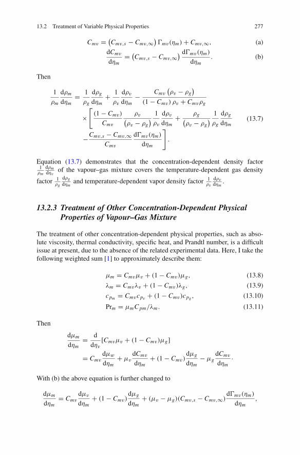
13.2 Treatment of Variable Physical Properties 277
Cmv = (Cmv,s − Cmv,∞)�mv(ηm)+ Cmv,∞, (a)
dCmv
dηm= (Cmv,s − Cmv,∞
) d�mv(ηm)
dηm. (b)
Then
1
ρm
dρm
dηm= 1
ρg
dρg
dηm+ 1
ρv
dρvdηm
− Cmv(ρv − ρg
)
(1 − Cmv) ρv + Cmvρg
×[(1 − Cmv)
Cmv
ρv(ρv − ρg
) 1
ρv
dρvdηm
+ ρg(ρv − ρg
) 1
ρg
dρg
dηm
−Cmv,s − Cmv,∞Cmv
d�mv(ηm)
dηm
].
(13.7)
Equation (13.7) demonstrates that the concentration-dependent density factor1ρm
dρmdηv
of the vapour–gas mixture covers the temperature-dependent gas density
factor 1ρg
dρgdηm
and temperature-dependent vapor density factor 1ρv
dρvdηm
.
13.2.3 Treatment of Other Concentration-Dependent PhysicalProperties of Vapour–Gas Mixture
The treatment of other concentration-dependent physical properties, such as abso-lute viscosity, thermal conductivity, specific heat, and Prandtl number, is a difficultissue at present, due to the absence of the related experimental data. Here, I take thefollowing weighted sum [1] to approximately describe them:
μm = Cmvμv + (1 − Cmv)μg, (13.8)
λm = Cmvλv + (1 − Cmv)λg, (13.9)
cpm = Cmvcpv + (1 − Cmv)cpg , (13.10)
Prm = μmC pm/λm . (13.11)
Then
dμm
dηm= d
dηv[Cmvμv + (1 − Cmv)μg]
= Cmvdμwdηm
+ μvdCmv
dηm+ (1 − Cmv)
dμg
dηm− μg
dCmv
dηm·
With (b) the above equation is further changed to
dμm
dηm= Cmv
dμvdηm
+ (1 − Cmv)dμg
dηm+ (μv − μg)(Cmv,s − Cmv,∞)
d�mv(ηm)
dηm,
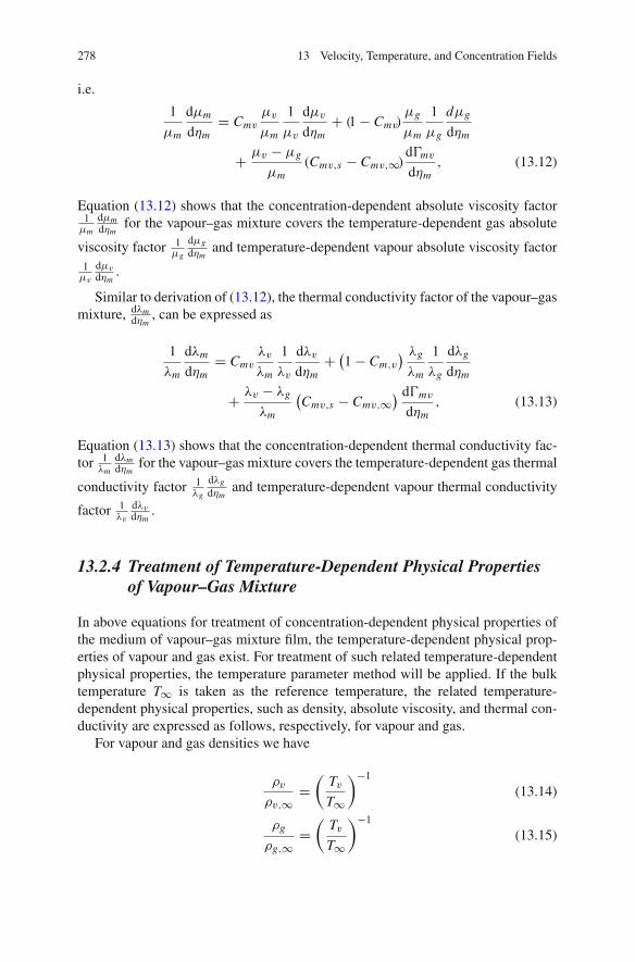
278 13 Velocity, Temperature, and Concentration Fields
i.e.
1
μm
dμm
dηm= Cmv
μv
μm
1
μv
dμvdηm
+ (1 − Cmv)μg
μm
1
μg
dμg
dηm
+ μv − μg
μm(Cmv,s − Cmv,∞)
d�mv
dηm, (13.12)
Equation (13.12) shows that the concentration-dependent absolute viscosity factor1μm
dμmdηm
for the vapour–gas mixture covers the temperature-dependent gas absolute
viscosity factor 1μg
dμgdηm
and temperature-dependent vapour absolute viscosity factor1μv
dμvdηm
.
Similar to derivation of (13.12), the thermal conductivity factor of the vapour–gasmixture, dλm
dηm, can be expressed as
1
λm
dλm
dηm= Cmv
λv
λm
1
λv
dλvdηm
+ (1 − Cm,v) λg
λm
1
λg
dλg
dηm
+ λv − λg
λm
(Cmv,s − Cmv,∞
) d�mv
dηm, (13.13)
Equation (13.13) shows that the concentration-dependent thermal conductivity fac-tor 1
λm
dλmdηm
for the vapour–gas mixture covers the temperature-dependent gas thermal
conductivity factor 1λg
dλgdηm
and temperature-dependent vapour thermal conductivity
factor 1λv
dλvdηm
.
13.2.4 Treatment of Temperature-Dependent Physical Propertiesof Vapour–Gas Mixture
In above equations for treatment of concentration-dependent physical properties ofthe medium of vapour–gas mixture film, the temperature-dependent physical prop-erties of vapour and gas exist. For treatment of such related temperature-dependentphysical properties, the temperature parameter method will be applied. If the bulktemperature T∞ is taken as the reference temperature, the related temperature-dependent physical properties, such as density, absolute viscosity, and thermal con-ductivity are expressed as follows, respectively, for vapour and gas.
For vapour and gas densities we have
ρv
ρv,∞=(
TvT∞
)−1
(13.14)
ρg
ρg,∞=(
TvT∞
)−1
(13.15)

13.2 Treatment of Variable Physical Properties 279
For vapour and gas absolute viscosities we have
μv
μv,∞=(
T
T∞
)nμ,v(13.16)
μg
μg,∞=(
T
T∞
)nμ,g(13.17)
For vapour and gas thermal conductivities we have
λv
λv,∞=(
T
T∞
)nλ,v(13.18)
λg
λg,∞=(
T
T∞
)nλ,g(13.19)
where nμ,v and nμ,g denote viscosity parameters of vapour and gas, respectively,and λμ,v and λμ,g denote thermal conductivity parameters of vapour and gas,respectively.
With (12.22) and (12.24), the vapour and gas physical property factors arederived as follows based on the above equations:
For density factors
1
ρv
dρvdηm
= − (Ts,int/T∞ − 1)dθm/dηm
(Ts,int/T∞ − 1)θm + 1(13.20)
1
ρg
dρg
dηm= − (Ts,int/T∞ − 1)dθm/dηm
(Ts,int/T∞ − 1)θm + 1(13.21)
For absolute viscosity factors
1
μv
dμvdηm
= nμ,v(Ts,int/T∞ − 1)dθm/dηm
(Ts,int/T∞ − 1)θm + 1(13.22)
1
μg
dμg
dηm= nμ,g(Ts,int/T∞ − 1)dθm/dηm
(Ts,int/T∞ − 1)θm + 1(13.23)
For thermal conductivity factors
1
λv
dλvdηm
= nλ,v(Ts,int/T∞ − 1)dθm/dηm
(Ts,int/T∞ − 1)θm + 1(13.24)
1
λg
dλg
dηm= nλ,g(Ts,int/T∞ − 1)dθm/dηm
(Ts,int/T∞ − 1)θm + 1(13.25)

280 13 Velocity, Temperature, and Concentration Fields
So far, the set of equations of the physical property factors involed in the similaritymathematical model of laminar forced film condensation of vapour–gas mixture arecompletely described on temperature-dependent physical properties of the liquidfilm medium and the temperature and concentration-dependent physical propertiesof the vapour–gas mixture film media. All these are basis for rigorous and reliablenumerical solution of the governing mathematical model of laminar forced film con-densation of vapour–gas mixture.
13.3 Numerical Calculation Procedure
Although a solution of the governing equations for laminar film condensation ofvapour is a difficult issue, the solution for the film condensation of vapour–gasmixture is even a challenge. The biggest challenge of the solution is to satisfy thewhole set of the matching conditions between the liquid–vapour interface (for short,interfacial matching conditions). To this end, some of our previous literatures havedealt with this issue for laminar-free film condensation of pure vapour [2–4] aswell as for laminar-free film condensation of vapour–gas mixture [1]. Furthermore,in Chap. 10, I obtained the solution for laminar forced film condensation of purevapour. In this chapter, I will further treat the challenging issue on solution of lami-nar forced film condensation of vapour–gas mixture. The whole solution is dividedinto the following steps:
Step 1: Calculation for liquid filmIn the first step, the governing equations of liquid film are calculated. The solu-tions of (12.28), (12.39), and (12.30) are found out by using boundary conditionequations (12.35), as well as the supposed initial values of condensate liquid filmthickness ηlδ and liquid interfacial velocity component Wxl,s as the boundary con-ditions. Then, the second step of calculation begins.
Step 2: Calculation for vapour filmIn this step of calculation, first (12.36) and (12.37) are used for evaluation of Wxv,sand Wxv,s respectively by using the solutions of Wxl,s and Wxy,s obtained from thestep 1. Then, with equations (12.40), (12.41), and (12.43), as well as the evaluatedvalues of Wxv,s and Wxv,s as the boundary conditions, (12.31), (12.32), (12.33), and(12.34) are solved.
Step 3: Judgment on the convergence of the numerical calculationIn this step of calculation, first (12.38), (12.39), and (12.42) are applied as judgmentequations for verification of the solution convergence. By means of these judgmentequations, the calculation is iterated with appropriate change of the values ηlδ andWxl,s . In each iteration, calculation on step 1 for liquid film equations (12.28),(12.29), and (12.30) and calculation on step 2 for vapour film equations (12.31),(12.32), (12.33), and (12.34) are done successively. In each step of calculations, thegoverning equations are solved by a shooting method with seventh-order Runge-Kutta integration. For solving such very strong nonlinear problem, a special variable

13.4 Numerical Solutions 281
mesh approach is applied to the numerical calculation programs, in order to obtainaccurate numerical solutions.
It should be emphasized that satisfying all interfacial physical matching con-ditions is important for obtaining reliable solutions for the laminar forced filmcondensation with two-phase flows. Even one of the interfacial physical matchingconditions is ignored, the solutions will be multiple, and it is never possible to obtainthe sole set of correct solutions.
13.4 Numerical Solutions
13.4.1 Interfacial Vapour Saturation Temperature
The interfacial saturation temperature Ts,int of the vapour–gas mixture depends onthe interfacial vapour mass fraction Cmv,s . In this present work, the laminar forcedfilm condensation of water vapour in the presence of air is taken as example forthe numerical calculation. The vapour–gas mixture temperature in the bulk is setas t∞ = 100 ◦C. According to the experimental data, the following equation [1] istaken for determination of the interfacial water vapour condensate saturated temper-ature Ts,int dependent on its interfacial vapour mass fraction Cmv,s at atmosphericpressure as the system pressure:
Ts,int = Ts · Cmv,s0.063, (13.26)
where Ts = 373 K is the vapour saturation temperature (with Cmv,s = 1) at theatmospheric pressure as the system pressure.
It should be indicated that according to the experimental data, for any systempressure the relationship of the interfacial saturation temperature Ts,int to its inter-facial vapour mass fraction is similar to that shown in (13.26). Here in this book,the pressure in the system is taken as atmospheric pressure, and (13.26) keep validin this case.
Equation (13.26) shows that the interfacial vapour mass fraction Cmv,s domi-nates the interfacial vapour saturation temperature. However, Cmv,s is solution ofthe governing equations and found out in iterative process for solving the governingequations.
13.4.2 Effect of the Interfacial Vapour Saturation Temperatureon Wall Subcooled Temperature
For laminar forced film condensation of water vapour in the presence of air on ahorizontal flat plate, a system of numerical calculations is carried out for differentwall temperatures tw and water vapour bulk mass fraction, Cmv,∞. According toChap. 7, the absolute viscosity parameters nμ,v and nμ,g are taken as nμ,v = 1.04

282 13 Velocity, Temperature, and Concentration Fields
and nλ,v = 1.185, respectively, for water vapour and air, and thermal conductivityparameters nλ,v and nλ,g are taken as nμ,g = 0.68 and nλ,g = 0.81, respectively,for water vapour and air, in the numerical calculation. While the water vapour massdiffusion coefficient in air is taken as 0.256 × 10⁻⁴, m2/s, and the latent heat ofwater vapour condensation is taken as h fg = 2257.3 kJ/kg.
With the numerical solutions on interfacial vapour saturation temperature ts,intfor laminar forced film condensation of water vapour–gas mixture with the bulktemperature t∞ = 100◦C and at atmosphere as the system pressure, the wall sub-cooled temperature ts,int − tw is found out, and shown in Fig. 13.1 with variationsof wall temperature and interfacial vapour mass fraction Cmv,s . Obviously, with aspecial wall temperature, the wall subcooled temperature ts,int − tw depends on theinterfacial vapour saturation temperature ts,int. It is seen from Fig. 13.1 that withdecreasing the interfacial vapour mass fraction Cmv,s , the wall subcooled temper-ature ts,int − tw will decrease at an accelerative pace, and such decreasing will beeven obvious with decreasing the wall temperature tw. Since the wall subcooledtemperature is the force of the condensate heat band mass transfer, such effect ofthe interfacial vapour saturation temperature on the wall subcooled temperature willdominate the condensate heat and mass transfer.
Fig. 13.1 Evaluated wallsubcooled temperaturets,int − tw with different walltemperature tw and interfacialvapour mass faction Cmv,s forlaminar forced filmcondensation of watervapour–gas mixture with thebulk temperaturet∞ = 100◦C and atatmosphere as the systempressure
0
20
40
60
80
100
0 0.2 0.4 0.6 0.8 1
Cmv,s
t s,in
t − t w
tw = 99 oCtw = 90 oC
tw = 80 oC
tw = 40 oC
tw = 20 oCtw = 10 oCtw = 0 oC
tw = 60 oC
13.4.3 Velocity, Concentration, and Temperature Fieldsof the Two-Phase Film Flows
The laminar forced film condensation of water vapour in the presence of air on a hor-izontal flat plate is taken as an example for the practical solution. The given condi-tions for solution are wall temperatures tw and the bulk vapour mass fraction Cmv,∞with the bulk temperature t∞ = 100◦C and at atmosphere as the system pressure.
With the available numerical procedure, the governing ordinary equations(12.28), (12.29), (12.30), (12.31), (12.32), (12.33), and (12.34), the boundary con-ditions, (12.35), (12.36), (12.37), (12.38), (12.39), (12.40), (12.41), (12.42), and

13.4 Numerical Solutions 283
0
0.02
0.04
0.06
0.08
0.1
0.12
0 0.2 0.4 0.6 0.8 1 1.2 1.4 1.6
lη
lη
1
11
oCtw 0 = o
Ctw 0 =W
xl (
η l)
(a)
0
0.2
0.4
0.6
0.8
1
0 0.2 0.4 0.6 0.8 1 1.2 1.4 1.6
1
11
θ l (η l)
(b)
Fig. 13.2 Numerical results of (a) velocity Wxl (ηl) and (b) temperature θl (ηl) profiles of liquidfilm for laminar forced film condensation of water–air mixture on a horizontal flat plate with tw =0◦C (lines 1 to 11 for Cmv,∞ = 0.1, 0.2, 0.3, 0.4, 0.5, 0.6, 0.7, 0.8, 0.9, 0.95, and 0.99. respectively)
0
0.2
0.4
0.6
0.8
0 0.2 0.4 0.6 0.8 1 1.2 1.4 1.6
11
11
Wxv
(ηv)
(a)
0 0.2 0.4 0.6 0.8 1 1.2 1.4 1.60
0.2
0.4
0.6
0.8
1
111
tw = 0o C
)( v
vη
θ
(b)
ηv
ηv
ηv
0 0.2 0.4 0.6 0.8 1 1.2 1.4 1.60
0.2
0.4
0.6
0.8
1
111
)(
,v
vm
ηΓ
(c)
tw = 0o C
tw = 0o C
Fig. 13.3 Numerical results on (a) velocity component Wxv(ηv), (b) temperature θv(ηv), and (c)relative concentration �m,v(ηv) profiles of vapour–gas mixture film for laminar forced film conden-sation of water-air mixture on a horizontal flat plate with tw = 0◦C (lines 1 to 11 for Cmv,∞ = 0.1,0.2, 0.3, 0.4, 0.5, 0.6, 0.7, 0.8, 0.9, 0.95, and 0.99. respectively)
(12.43), and the physical property equations (13.7), (13.8), (13.9), (13.10), (13.11),(13.12), and (13.13), and (13.20), (13.21), (13.22), (13.23), (13.24), and (13.25)are rigorously calculated, and a system of solutions for velocity, concentration, andtemperature fields is obtained, and plotted in Figs. 13.2, 13.3, 13.4, 13.5, 13.6, 13.7,13.8, and 13.9 with variation of the wall temperatures tw and bulk vapour mass frac-tion Cmv,∞, respectively. From Figs. 13.1, 13.2, 13.3, 13.4, 13.5, 13.6, 13.7, 13.8,

284 13 Velocity, Temperature, and Concentration Fields
(a)
0
0.02
0.04
0.06
0.08
0.1
0.12
ηl
1
10
2
tw = 40 CW
xl (
η l)
0 0.2 0.4 0.6 0.8 1 1.2 1.4 1.60
0.2
0.4
0.6
0.8
1
0 0.2 0.4 0.6 0.8 1 1.2 1.4 1.6ηl
1
10θ l (η
l)
(b)
tw = 40o
Co
Fig. 13.4 Numerical results of (a) velocity Wxl (ηl) and (b) temperature θl (ηl) profiles of liquidfilm for laminar forced film condensation of water–air mixture on a horizontal flat plate with tw =40◦C (lines 1 to 10 for Cmv,∞ = 0.2, 0.3, 0.4, 0.5, 0.6, 0.7, 0.8, 0.9, 0.95, and 0.99. respectively)
(a)
0
0.2
0.4
0.6
0.8
1 1
ηv
10tw = 40o C
Wx
v (η
v)
0 0.2 0.4 0.6 0.8 1 1.2 1.4 1.6
(b)
ηv
θ v (η
v)
0
0.2
0.4
0.6
0.8
1
0 0.2 0.4 0.6 0.8 1 1.2 1.4 1.61
10
0
0.2
0.4
0.6
0.8
1
0 0.2 0.4 0.6 0.8 1 1.2 1.4 1.6
110
Γ m,v
(η v
)
(c)
ηv
tw = 40o C
tw = 40o C
Fig. 13.5 Numerical results of (a) velocity component Wxv(ηv), (b) temperature θv(ηv), and (c)relative concentration �m,v(ηv) profiles of vapour–gas mixture film for laminar forced film conden-sation of water-air mixture on a horizontal flat plate with tw = 40◦C (lines 1 to 10 for Cmv,∞ = 0.2,0.3, 0.4, 0.5, 0.6, 0.7, 0.8, 0.9, 0.95, and 0.99. respectively)
and 13.9 it is seen that the following effect of the given conditions tw and Cmv,∞ onvelocity and temperature fields of the two-phase forced film condensation.
First, it is found that the bulk vapour mass fraction Cmv,∞ has a decisive effecton the laminar forced film condensation of vapour–gas mixture, and decreasing thebulk vapour mass fraction Cmv,∞ (i.e. increasing the bulk gas mass fraction) causes

13.4 Numerical Solutions 285
0
0.02
0.04
0.06
0.08
0.1
0.12
0 0.2 0.4 0.6 0.8 1 1.2 1.4 1.6
1
ηl ηl
tw = 60o C
6
(a)
0
0.2
0.4
0.6
0.8
1
0 0.2 0.4 0.6 0.8 1 1.2 1.4 1.6
1
6
(b)
tw = 60o C
Wx
l (η l)
θ l (η
l)
Fig. 13.6 Numerical results of (a) velocity Wxl (ηl) and (b) temperature θl (ηl) profiles of liquidfilm for laminar forced film condensation of water–air mixture on a horizontal flat plate with tw =60◦C (lines 1 to 6 for Cmv,∞ = 0.6, 0.7, 0.8, 0.9, 0.95, and 0.99. respectively)
0
0.2
0.4
0.6
0.8
1
0 0.2 0.4 0.6 0.8 1 1.2 1.4 1.6
vη
1 6
)(
,v
vm
ηΓ
(c)
0
0.2
0.4
0.6
0.8
1
vη
(a)
0 0.2 0.4 0.6 0.8 1 1.2 1.4 1.60
0.2
0.4
0.6
0.8
1
vη
1 6
(b)
0 0.2 0.4 0.6 0.8 1 1.2 1.4 1.6
θ v (η
v)
Wx
v (η
v)
tw = 60
o C
tw = 60
o C
tw = 60
o C
Fig. 13.7 Numerical results of (a) velocity component Wxv(ηv), (b) temperature θv(ηv), and (c)relative concentration �m,v(ηv) profiles of vapour–gas mixture film for laminar forced film conden-sation of water–air mixture on a horizontal flat plate with tw = 60◦C (lines 1 to 6 for Cmv,∞ = 0.6,0.7, 0.8, 0.9, 0.95, and 0.99. respectively)
(1) decreasing the condensate liquid film thickness;(2) increasing the condensate liquid film temperature gradient;(3) decreasing the wall subcooled temperature ts,int − tw at an accelerative pace,
which will lead to decreasing the condensate heat transfer at an accelerativepace;

286 13 Velocity, Temperature, and Concentration Fields
0
0.02
0.04
0.06
0.08
0.1
0.12
0 0.2 0.4 0.6 0.8 1 1.2 1.4 1.6ηl
12
3
4
5
Wxl
(ηl)
(a)
ηl
(b)
0 0.2 0.4 0.6 0.8 1 1.2 1.4 1.60
0.2
0.4
0.6
0.8
1
1
5
θ l (η l
)
Cmv,∞ = 0.9Cmv,∞
= 0.9
Fig. 13.8 Numerical results of (a) velocity Wxl (ηl) and (b) temperature θl(ηl ) profiles of liq-uid film for laminar forced film condensation of water–air mixture on a horizontal flat plate withCmv,∞ = 0.9 (lines 1 to 5 for tw = 0, 20, 40, 60 and 80◦C, respectively)
0 0.2 0.4 0.6 0.8 1 1.2 1.4 1.60
0.2
0.4
0.6
0.8
1Cmv,∞ = 0.9
1
5
Γ m,v
(ηv)
(c)ηv
0
0.2
0.4
0.6
0.8
1
0 0.2 0.4 0.6 0.8 1 1.2 1.4 1.6
1
5
Wxv
(ηv)
(a) (b)
Cmv,∞ = 0.9
0 0.2 0.4 0.6 0.8 1 1.2 1.4 1.60
0.2
0.4
0.6
0.8
1
1
5
θ v (
η v)
ηv
Cmv,∞ = 0.9
ηv
Fig. 13.9 Numerical results of (c) velocity component Wxv(ηv), (d) temperature θv(ηv), and (e)relative concentration �m,v(ηv) profiles of vapour–gas mixture film for laminar forced film con-densation of water-air mixture on a horizontal flat plate with Cmv,∞ = 0.9 (lines 1 to 5 for tw = 0,20, 40, 60 and 80◦C, respectively)
(4) increasing the vapour–gas mixture film flow velocity level;(5) increasing the temperature gradient of the vapour–gas mixture film;(6) decreasing the vapour–gas mixture velocity, concentration, and temperature
boundary layer thicknesses.
13.5 Remarks 287
While, increasing the wall temperature tw causes
(1) decreasing the condensate liquid film thickness obviously;(2) decreasing the condensate liquid film velocity level at an accelerative pace;(3) increasing the wall temperature gradient obviously;(4) decreasing the wall subcooled temperature ts,int − tw obviously, which will lead
to decreasing the condensate heat transfer obviously;(5) decreasing the vapour–gas mixture film flow velocity level at an accelerative
pace;(6) decreasing the dimensionless temperature gradient of vapour–gas mixture film
flow at an accelerative pace;(7) increasing the vapour–gas mixture film flow velocity, concentration, and tem-
perature boundary layer thicknesses at an accelerative pace.
13.5 Remarks
In this chapter, a series of treatments of concentration and temperature-dependentphysical properties of the governing similarity mathematical model is done,before the numerical calculation. The physical property factors of liquid film aretemperature-dependent. The physical property factors of vapour–gas mixture filmare concentration-dependent in the governing similarity mathematical model; how-ever, after the analysis, it is found that they cover the temperature-dependent phys-ical property factors of vapour and gas. Obviously, the concentration-dependentphysical properties of vapour–gas mixture are closely dependent on the temperature-dependent physical properties of vapour and gas. Finally, a set of physical propertyfactors covered by the governing similarity mathematical model is transformed tothe functions of the dimensionless temperature and dimensionless concentration forconvenient numerical calculation. Seven matching conditions at the liquid–vaporinterface, including two-dimensional velocity component balances, shear force bal-ance, mass flow rate balance, temperature balance, heat transfer balance, concentra-tion condition, as well as the balance between the condensate mass flow and vapourmass diffusion are considered and rigorously satisfied in the numerical calculation.In fact, it is necessary to satisfy all these interfacial physical matching conditions forobtaining reliable solutions of the two-point boundary value problem for the laminarforced film condensation of vapour–gas mixture. Otherwise, it is never possible toobtain any reliable solution of the governing similarity mathematical model.
Furthermore, a useful approach is provided to rigorously determine the vapourcondensate saturated temperature ts,int at the liquid–vapour interface. While, thevapour condensate saturated temperature ts,int is dependent on interfacial vapourpartial pressure or vapour mass fraction. On this basis, the vapour condensate sat-urated temperature ts,int is evaluated iteratively by using the provided iterative pro-cedure. All these approaches lead to rigorous and reliable numerical results on thelaminar forced film condensation of vapour–gas mixture.
288 13 Velocity, Temperature, and Concentration Fields
The laminar forced film condensation of water vapour in the presence of air istaken as an example for the numerical calculation. A system of rigorous numericalresults is obtained, including velocity and temperature fields of the condensate liquidfilm, as well as the velocity, temperature and concentration fields of the vapour–gasmixture film. From these numerical results, it is found that the bulk vapour massfraction has a decisive effect on the laminar forced film condensation of vapour inthe presence of noncondensable gas, since the noncondensable gas strongly reducedthe wall subcooled temperature.
Furthermore, the effects of the given conditions, the bulk vapour mass fraction,and wall temperature on the two-phase film flow condensation of vapour–gas mix-ture are clarified in detail.
The bulk vapour mass fraction Cmv,∞ has a decisive effect on the laminar forcedfilm condensation of vapour–gas mixture. Decreasing the bulk vapour mass fractionCmv,∞ (i.e. increasing the bulk gas mass fraction) causes
(1) decreasing the condensate liquid film thickness;(2) increasing the condensate liquid film temperature gradient;(3) decreasing the wall subcooled temperature ts,int − tw at an accelerative pace,
which will lead to decreasing the condensate heat transfer at an accelerativepace;
(4) increasing the vapour–gas mixture film flow velocity level;(5) increasing the temperature gradient of the vapour–gas mixture film;(6) decreasing the vapour–gas mixture velocity, concentration, and temperature
boundary layer thicknesses.
While, increasing the wall temperature tw causes
(1) decreasing the condensate liquid film thickness obviously;(2) decreasing the condensate liquid film velocity level at an accelerative pace;(3) increasing the wall temperature gradient obviously;(4) decreasing the wall subcooled temperature ts,int − tw obviously, which will lead
to decreasing the condensate heat transfer obviously;(5) decreasing the vapour–gas mixture film flow velocity level at an accelerative
pace;(6) decreasing the temperature gradient of vapour–gas mixture film flow at an accel-
erative pace;(7) increasing the vapour–gas mixture film flow velocity, concentration, and tem-
perature boundary layer thicknesses at an accelerative pace.
The study results of this work for laminar forced film condensation from vapour–gas mixture can be taken as a basis on a successive investigation for its heat and masstransfer.
References 289
Exercises
1. Which parts of contents does the complete similarity governing mathematicalmodel cover for laminar forced film condensation of vapour–gas mixture?
2. Please provide the related physical analysis to explain the close relationshipbetween the concentration-dependent density of vapour–gas mixture and thetemperature-dependent densities of vapour and gas.
References
1. D.Y. Shang, L.C. Zhong, Extensive study on laminar free film condensation from vapor–gasmixture. Int. J. Heat Mass Transfer 51, 4300–4314 (2008)
2. D.Y. Shang, T. Adamek, Study on laminar film condensation of saturated steam on a vertical flatplate for consideration of various physical factors including variable thermophysical properties.Wärme- und Stoffübertragung 30, 89–100 (1994)
3. D.Y. Shang, B.X. Wang, An extended study on steady-state laminar film condensation of asuperheated vapor on an isothermal vertical plate. Int. J. Heat Mass Transfer 40(4), 931–941(1997)
4. D.Y. Shang, Free convection film flows and heat transfer (Springer-Verlag, Berlin, Heidelbergand New York, 2006)

Chapter 14Heat and Mass Transfer on Laminar ForcedFilm Condensation of Vapour–Gas Mixture
Abstract Through the heat and mass transfer analyses, the equations of condensateheat and mass transfer rates are provided, where only dimensionless wall tempera-ture gradient, interfacial vapour saturation temperature and defined condensate massflow rate parameter are non-given conditions. The defined mass flow rate parameterdepends on condensate liquid film thickness as well as the interfacial condensateliquid velocity components. Then, the laminar forced film condensation of watervapour in the presence of air on a horizontal flat plate is taken as an example,and a system of numerical results of the wall dimensionless temperature gradientand mass flow rate parameter are obtained. It is found that although decreasingthe bulk vapour mass fraction (i.e. increasing the bulk gas mass fraction) causesincrease of the wall dimensionless temperature gradient, it decreases the condensatemass flow rate parameter. However increasing the reference wall subcooled gradecauses decrease of the wall temperature gradient and increase of the condensatemass flow rate parameter. These phenomena are closely related to the effect of thenon-condensable gas on the condensation. The system of the rigorous key solutionsof the wall dimensionless temperature gradient and condensate mass flow rate para-mater is formulated using the simple and reliable equations for the laminar film con-densation of water vapour–air mixture on a horizontal flat plate. In combination withthe provided theoretical heat transfer equation, the formulated equation of the walldimensionless temperature gradient and condensate mass flow rate parameter canbe used for simple and reliable evaluation of the condensate heat transfer rate. Theinterfacial vapour saturation temperature, necessary for correct prediction of laminarfilm condensation of vapour–gas mixture, is deeply investigated here. By taking thelaminar forced film condensation of water vapour–air mixture as an example, threemethods are reported for evaluation of the interfacial vapour saturation temperature:(1) the numerical calculation method, (2) prediction with the formulation equationand (3) prediction by solving the condensate mass–energy transformation equation.The calculated results of the interfacial vapour saturation temperature related to dif-ferent methods are well coincident. It proves that the similarity analysis method, thesimilarity mathematical model, the numerical calculation and treatment method ofvariable physical properties reported in this chapter are valid for extensive investi-gation of heat and mass transfer of laminar forced film condensation of vapour–gas
D.Y. Shang, Theory of Heat Transfer with Forced Convection Film Flows,Heat and Mass Transfer, DOI 10.1007/978-3-642-12581-2_14,C© Springer-Verlag Berlin Heidelberg 2011
291
292 14 Heat and Mass Transfer on Laminar Forced Film Condensation
mixture. The author believes that the analysis and calculation methods reported inthis work can be conveniently extended to investigate other different types of lami-nar forced film condensation from vapour–gas mixture.
14.1 Introduction
In Chaps. 12 and 13, I presented the complete similarity mathematical model andthe numerical results of velocity, temperature and concentration fields on laminarforced film condensation from vapour–gas mixture, respectively. In this chapter,further investigation will be done for heat and mass transfer. For this purpose, theappropriate heat and mass transfer analyses will be done for providing the relatedappropriate theoretical equations. In these theoretical equations, the key solutions,i.e. the wall dimensionless temperature gradient and the induced condensate massflow rate parameter become the unknown variables on evaluation of condensate heatand mass transfer respectively. Furthermore, the key solutions to the wall dimen-sionless temperature gradient and the condensate mass flow rate parameter of thegoverning similarity mathematical model will be formulated based on the rigor-ous numerical results so that the theoretical equations of condensate heat and masstransfer can be conveniently used for simple and reliable prediction.
14.2 Heat Transfer Analysis
Consulting the related derivation in Chap. 11 for heat and mass transfer analyses oflaminar forced film condensation of pure vapour, the heat and transfer analyses ofthe laminar forced film condensation of vapour–gas mixture will be done briefly asbelow.
The local heat transfer rate qx,w with consideration of variable physical proper-ties for the film condensation at position x per unit area on the plate can be calculatedby applying Fourier’s law as
qx,w = −λl,w
(∂t
∂y
)
y=0
With (12.17), (12.18) and (12.19), qx,w is described as
qx,w = λl,w(tw − ts,int
) (1
2Rexl,s
)1/2
x−1(
−dθl (ηl)
dηl
)
ηl=0(14.1)
where the subscript w notes the local value at the wall with consideration of variablephysical properties and ts,int denotes the interfacial vapour saturation temperaturedependent on the interfacial vapour mass fraction Cmv,s.
Then, the local heat transfer coefficient, defined as qx,w = αx (tw − ts,int), will be
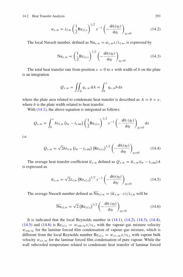
14.2 Heat Transfer Analysis 293
αx,w = λl,w
(1
2Rexl,s
)1/2
x−1(
−dθl(ηl)
dηl
)
ηl=0(14.2)
The local Nusselt number, defined as Nux,w = αx,wx/λl,w, is expressed by
Nux,w =(
1
2Rexl,s
)1/2 (−dθl(ηl)
dηl
)
ηl=0(14.3)
The total heat transfer rate from position x = 0 to x with width of b on the plateis an integration
Qx,w =∫∫
Aqx,w dA =
∫ x
0qx,wb dx
where the plate area related to condensate heat transfer is described as A = b × x ,where b is the plate width related to heat transfer.
With (14.1), the above equation is integrated as follows:
Qx,w =∫ x
0bλl,w
(tw − ts,int
) (1
2Rexl,s
)1/2
x−1(
−dθl (ηl)
dηl
)
ηl=0dx
i.e.
Qx,w = √2bλl,w
(tw − ts,int
) (Rexl,s
)1/2 (−dθl(ηl)
dηl
)
ηl=0(14.4)
The average heat transfer coefficient αx,w defined as Qx,w = αx,w(tw − ts,int)Ais expressed as
αx,w = √2λl,w
(Rexl,s
)1/2x−1(
−dθl(ηl)
dηl
)
ηl=0(14.5)
The average Nusselt number defined as Nuxl,w = (αx,w · x)/λl,w will be
Nuxl,w = √2(Rexl,s
)1/2 (−dθl (ηl)
dηl
)
ηl=0(14.6)
It is indicated that the local Reynolds number in (14.1), (14.2), (14.3), (14.4),(14.5) and (14.6) is Rexl,s = wxm,∞x/νl,s with the vapour–gas mixture velocitywxm,∞ for the laminar forced film condensation of vapour–gas mixture, which isdifferent from the local Reynolds number Rexl,s = wxv,∞x/νl,s with vapour bulkvelocity wxv,∞ for the laminar forced film condensation of pure vapour. While thewall subcooled temperature related to condensate heat transfer of laminar forced

294 14 Heat and Mass Transfer on Laminar Forced Film Condensation
film condensation of vapour–gas mixture is ts,int − tw, which strongly reduces thecondensate heat transfer due to the presence of the non-condensable gas.
From these theoretical equations of heat transfer, it is seen that there are twono-given variables for prediction of condensate heat transfer of the laminar forcedfilm condensation of vapour–gas mixture. They are wall dimensionless temperaturegradient
(−dθl (ηl)
dηl
)
ηl=0
and the interfacial vapour saturation temperature ts,int. In the next sections, the eval-uation approach of the two variables will be further investigated for prediction ofheat transfer of the laminar forced film condensation of vapour–gas mixture.
14.3 Wall Dimensionless Temperature Gradient
Equations (14.1), (14.2), (14.3), (14.4), (14.5) and (14.6) demonstrate that walldimensionless temperature gradient
(−dθl(ηl)
dηl
)
ηl=0
is a key solution of the governing similarity mathematical model for evaluation ofheat transfer of the film condensation of vapour–gas mixture.
The laminar forced film condensation of water vapour–air mixture on a horizontalflat plate is taken as an example for solution. A system of key numerical solutionsof the wall dimensionless temperature gradient
(−dθl (ηl)
dηl
)
ηl=0
are plotted in Fig. 14.1, and some of the typical solutions are listed in Table 14.1with variation of reference wall subcooled grade
(�tw)sts
(= ts − tw
ts
)
and bulk vapour mass fraction Cmv,∞. Here, ts is the reference vapour saturationtemperature (corresponding to Cmv,s = 1) and (�tw)s = ts − tw is defined asreference wall subcooled temperature (corresponding to Cmv,s = 1). The blankspace in Table 14.1 which is located above the lines of Fig. 14.1 is the region withts,int − tw < 0.
It is seen that decreasing the bulk vapour mass fraction causes increase of thewall dimensionless temperature gradient at an accelerative pace. On the other hand,

14.3 Wall Dimensionless Temperature Gradient 295
Tabl
e14
.1N
umer
ical
resu
lts
( −dθl(η
l)
dηl
) ηl=
0of
lam
inar
forc
edfil
mco
nden
satio
nof
wat
erva
pour
–air
mix
ture
ona
hori
zont
alfla
tpla
teat
bulk
tem
pera
ture
t ∞=
100◦
C(T
hebl
ank
spac
ein
the
tabl
eco
rres
pond
sto
the
non-
cond
ensa
ble
regi
onw
ithth
ew
alls
ubco
oled
tem
pera
ture�
t w=
t s,i
nt−
t w<
0)
Cm,v
∞ 0.4
0.5
0.6
0.7
0.8
0.9
0.99
0.99
9
(�t w) s/
t st w
(◦C
)Ty
peof
data
−( dθ
l
dηl) η
l=0
0.05
95(1
)1.
6342
551.
5990
03(2
)R
egio
nfo
r�
t w=
t s,i
nt−
t w<
01.
6084
371.
5682
07(3
)−0.0
158
−0.0
1926
0.08
92(1
)R
egio
nfo
r�
t w=
t s,i
nt−
t w<
01.
6124
571.
3429
831.
3241
67(2
)1.
6405
721.
3669
571.
3434
79(3
)0.
0174
360.
0178
510.
0145
840.
1387
(1)
Reg
ion
for�
t w=
t s,i
nt−
t w<
01.
4953
191.
2676
591.
1388
751.
1278
9(2
)1.
5265
691.
3109
141.
1589
151.
1454
33(3
)0.
0208
980.
0341
220.
0175
970.
0155
540.
280
(1)
Reg
ion
for�
t w=
t s,i
nt−
t w<
01.
6759
391.
3798
821.
2158
861.
1084
1.03
661.
0274
(2)
1.62
0295
1.40
4829
1.24
1487
1.11
3247
1.01
9238
1.01
0736
(3)
−0.0
332
0.01
8079
0.02
1055
0.00
4373
−0.0
1675
−0.0
1622
0.4
60(1
)1.
5979
1.39
991.
2604
1.15
391.
069
0.99
820.
9436
0.93
84(2
)1.
6532
111.
4419
551.
2895
491.
1733
291.
0811
551.
0058
820.
9488
250.
9435
78(3
)0.
0346
150.
0300
420.
0231
260.
0168
370.
0113
710.
0076
960.
0055
370.
0055
180.
640
(1)
1.43
071.
2659
1.14
5606
1.05
450.
9815
0.91
810.
8698
0.86
53(2
)1.
4228
041.
2643
641.
1480
981.
0581
780.
9859
990.
9264
30.
8808
720.
8766
64(3
)−0.0
0552
−0.0
0121
0.00
2175
0.00
3488
0.00
4583
0.00
9073
0.01
2729
0.01
3133
0.8
20(1
)1.
291.
1488
1.04
560.
9653
0.90
020.
8454
0.80
260.
7986
(2)
1.32
3317
1.17
4005
1.06
4604
0.98
010.
9123
40.
8564
710.
8137
760.
8098
35(3
)0.
0258
270.
0219
410.
0181
760.
0153
320.
0134
860.
0130
960.
0139
250.
0140
681
0(1
)1.
1691
1.04
730.
9575
0.88
720.
8298
0.78
140.
7434
0.73
98(2
)1.
1706
091.
0477
960.
9570
780.
8865
330.
8296
410.
7824
970.
7463
160.
7429
69(3
)0.
0012
90.
0004
73−0.0
0044
−0.0
0075
−0.0
0019
0.00
1404
0.00
3923
0.00
4284
Not
e:(1
)nu
mer
ical
solu
tions
,(2)
resu
ltsev
alua
ted
by(1
4.7)
,and
(3)
devi
atio
nev
alua
ted
by(1
4.7)

296 14 Heat and Mass Transfer on Laminar Forced Film Condensation
Fig. 14.1 Numerical results(− dθl (ηl )
dηl
)ηl=0 of laminar
forced film condensation ofwater vapour-air mixture on ahorizontal flat plate at bulktemperature t∞ = 100◦C(lines 1 → 8 denote thereference wall subcooledgrade(�tw)s
ts
(= ts−tw
ts
)= 0.05,
0.08, 0.13, 0.2, 0.4, 0.6, 0.8and 1, respectively)
0.5
1
1.5
2
2.5
3
3.5
0 0.2 0.4 0.6 0.8 1
12
34
5
6
7
8
Cmv, ∞
This blank space is for
−)
(dη
l
dθl(
η l)η l=
0
ts, int − tw < 0
increasing the reference wall subcooled grade will cause decrease of the wall dimen-sionless temperature gradient. These phenomena will dominate condensate heattransfer of the laminar forced film condensation of vapour–gas mixture.
Furthermore, the rigorous numerical solutions of the wall dimensionless tem-perature gradient (dθl/dηl)ηl=0 of laminar forced film condensation of water–airmixture on a horizontal flat plate are formulated by using a curve-fitting approach,and the formulated equation of
(−dθl (ηl)
dηl
)
ηl=0
is shown below with the bulk vapour mass fraction and the reference wall subcooledgrade:
−(
dθl
dηl
)
ηl=0= ACmv,∞B (
0.4 ≤ Cmv,∞ ≤ 0.999)
(14.7)
where
A = 0.5868
[(�tw)s
ts
]−0.3272 (0.05 ≤ (�tw)s
ts≤ 0.2
)
A = − 0.334(�tw)s
ts+ 1.0766
(0.2 ≤ (�tw)s
ts≤ 1
)
B = − 0.2486
[(�tw)s
ts
]−0.8082 (0.05 ≤ (�tw)s
ts≤ 0.2
)
B = 2.8813
[(�tw)s
ts
]3
− 6.3245
[(�tw)s
ts
]2
+ 4.5528(�tw)s
ts− 1.6063
(0.2 ≤ (�tw)s
ts≤ 1
)

14.4 Determination of Interfacial Vapour Saturation Temperature 297
The results of the wall dimensionless temperature gradient
(−dθl (ηl)
dηl
)
ηl=0
predicted by using (14.7) are listed in Table 14.1. It is seen that the predicted valueof
(−dθl (ηl)
dηl
)
ηl=0
is very well coincident to the related numerical solutions. Therefore, (14.7) is reli-able for laminar forced film condensation of water–air mixture on a horizontal flatplate.
14.4 Determination of Interfacial Vapour SaturationTemperature
The prerequisite of correct determination of the interfacial vapour saturation tem-perature ts,int is the correct prediction of the corresponding interfacial vapour massfraction Cmv,s. With the numerical calculation in Chap. 13, a system of values ofthe interfacial vapour mass fraction Cmv,s have been obtained for the laminar filmcondensation of water vapour–air mixture on a horizontal flat plate. Now, these cal-culated results of the interfacial vapour mass fraction Cmv,s are plotted in Fig. 14.2with the related reference wall subcooled grade and bulk vapour mass fraction, and
0
0.1
0.2
0.3
0.4
0.5
0.6
0.7
0.8
0.9
0 0.2 0.4 0.6 0.8 1
1
2
3
4
5
67, 8
Cm
v, s
This blank space is for ts,int−tw< 0
Cmv,∞
Fig. 14.2 Numerical results of interfacial vapour mass fraction Cmv,s of the laminar film conden-sation of water vapour–air mixture on a horizontal flat plate at bulk temperature t∞ = 100◦C (lines1 → 8 denote the reference wall subcooled grade (�tw)s
ts= 0.05, 0.08, 0.13, 0.2, 0.4, 0.6, 0.8 and
1, respectively)
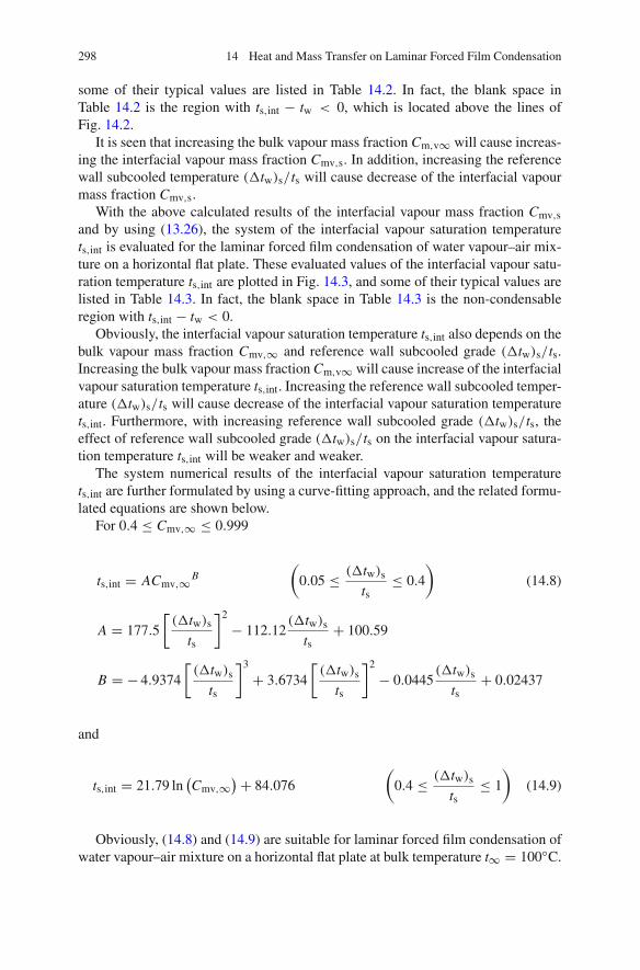
298 14 Heat and Mass Transfer on Laminar Forced Film Condensation
some of their typical values are listed in Table 14.2. In fact, the blank space inTable 14.2 is the region with ts,int − tw < 0, which is located above the lines ofFig. 14.2.
It is seen that increasing the bulk vapour mass fraction Cm,v∞ will cause increas-ing the interfacial vapour mass fraction Cmv,s. In addition, increasing the referencewall subcooled temperature (�tw)s/ts will cause decrease of the interfacial vapourmass fraction Cmv,s.
With the above calculated results of the interfacial vapour mass fraction Cmv,sand by using (13.26), the system of the interfacial vapour saturation temperaturets,int is evaluated for the laminar forced film condensation of water vapour–air mix-ture on a horizontal flat plate. These evaluated values of the interfacial vapour satu-ration temperature ts,int are plotted in Fig. 14.3, and some of their typical values arelisted in Table 14.3. In fact, the blank space in Table 14.3 is the non-condensableregion with ts,int − tw < 0.
Obviously, the interfacial vapour saturation temperature ts,int also depends on thebulk vapour mass fraction Cmv,∞ and reference wall subcooled grade (�tw)s/ts.Increasing the bulk vapour mass fraction Cm,v∞ will cause increase of the interfacialvapour saturation temperature ts,int. Increasing the reference wall subcooled temper-ature (�tw)s/ts will cause decrease of the interfacial vapour saturation temperaturets,int. Furthermore, with increasing reference wall subcooled grade (�tw)s/ts, theeffect of reference wall subcooled grade (�tw)s/ts on the interfacial vapour satura-tion temperature ts,int will be weaker and weaker.
The system numerical results of the interfacial vapour saturation temperaturets,int are further formulated by using a curve-fitting approach, and the related formu-lated equations are shown below.
For 0.4 ≤ Cmv,∞ ≤ 0.999
ts,int = ACmv,∞B(
0.05 ≤ (�tw)sts
≤ 0.4
)(14.8)
A = 177.5
[(�tw)s
ts
]2
− 112.12(�tw)s
ts+ 100.59
B = − 4.9374
[(�tw)s
ts
]3
+ 3.6734
[(�tw)s
ts
]2
− 0.0445(�tw)s
ts+ 0.02437
and
ts,int = 21.79 ln(Cmv,∞
)+ 84.076
(0.4 ≤ (�tw)s
ts≤ 1
)(14.9)
Obviously, (14.8) and (14.9) are suitable for laminar forced film condensation ofwater vapour–air mixture on a horizontal flat plate at bulk temperature t∞ = 100◦C.
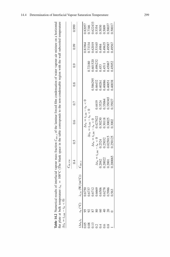
14.4 Determination of Interfacial Vapour Saturation Temperature 299
Tabl
e14
.2N
umer
ical
resu
ltsof
inte
rfac
ial
vapo
urm
ass
frac
tion
Cm
v,s
ofth
ela
min
arfo
rced
film
cond
ensa
tion
ofw
ater
vapo
ur–a
irm
ixtu
reon
aho
rizo
ntal
flat
plat
eat
bulk
tem
pera
ture
t ∞=
100◦
C(T
hebl
ank
spac
ein
the
tabl
eco
rres
pond
sto
the
non-
cond
ensa
ble
regi
onw
ithth
ew
all
subc
oole
dte
mpe
ratu
re�
t w=
t s,i
nt−
t w<
0)
Cm,v
∞0.
40.
50.
60.
70.
80.
90.
990.
999
(�t w) s
t w(◦
C)
λl,
w(W/(m
◦ C))
Cm
v,s
0.05
950.
6750
�t w
=t s,i
nt−
t w<
00.
8196
40.
8205
70.
0892
0.67
37�
t w=
t s,i
nt−
t w<
00.
7218
00.
7333
40.
7346
0.13
870.
6712
�t w
=t s,i
nt−
t w<
00.
5862
950.
6015
200.
6201
90.
6224
330.
280
0.66
69�
t w=
t s,i
nt−
t w<
00.
4278
220.
4419
0.46
432
0.49
6232
0.53
165
0.53
540.
460
0.65
060.
2042
0.25
240.
3023
00.
3524
0.40
261
0.45
30.
4984
0.50
300.
640
0.62
780.
2002
20.
2503
20.
3011
80.
3506
40.
4008
60.
4511
0.49
635
0.50
090.
820
0.59
860.
2001
0.02
5015
0.30
025
0.35
0365
0.40
051
0.45
067
0.49
587
0.50
037
10
0.56
30.
2000
650.
2501
250.
3002
0.35
027
0.40
038
0.45
052
0.49
567
0.50
017

300 14 Heat and Mass Transfer on Laminar Forced Film Condensation
Fig. 14.3 Numerical resultsof interfacial vapoursaturation temperature ts,int ofthe laminar film condensationof water vapour–air mixtureon a horizontal flat plate atbulk temperaturet∞ = 100◦C (lines 1 → 8denote wall subcooled grade(�tw)s/ts = 0.05, 0.08, 0.13,0.2, 0.4, 0.6, 0.8 and 1,respectively)
20
40
60
80
100
0 2.0 0.4 0.6 0.8 1
123
4
5
6
7,8
Cmv, ∞
t s, in
t o C
This blank space is for ts, int − tw < 0
The values of the interfacial vapour saturation temperature ts,int predicted byusing (14.8) and (14.9), and the relative predicted deviation from the numericalresults are listed in Table 14.3. It is seen that the predicted values are in very goodagreement with the related numerical results.
14.5 Simple and Reliable Prediction Equations of Heat Transfer
With the formulated equation (14.7), the theoretical equations (14.1), (14.2), (14.3),(14.4), (14.5) and (14.6) become available for prediction of heat transfer of laminarforced film condensation of water vapour–air mixture on a horizontal flat plate. Forexample (14.4) and (14.6) become:
Qx = √2bλl,w
(tw − ts,int
) (Rexl,s
)1/2ACmv,∞B (
0.4 ≤ Cmv,∞ ≤ 0.999)
(14.10)
Nuxl,w = √2(Rexl,s
)1/2ACmv,∞B (0.4 ≤ Cmv,∞ ≤ 0.999) (14.11)
where
A = 0.5868
[(�tw)s
ts
]−0.3272 (0.05 ≤ (�tw)s
ts≤ 0.2
)
A = −0.334(�tw)s
ts+ 1.0766
(0.2 ≤ (�tw)s
ts≤ 1
)
B = −0.2486
[(�tw)s
ts
]−0.8082 (0.05 ≤ (�tw)s
ts≤ 0.2
)
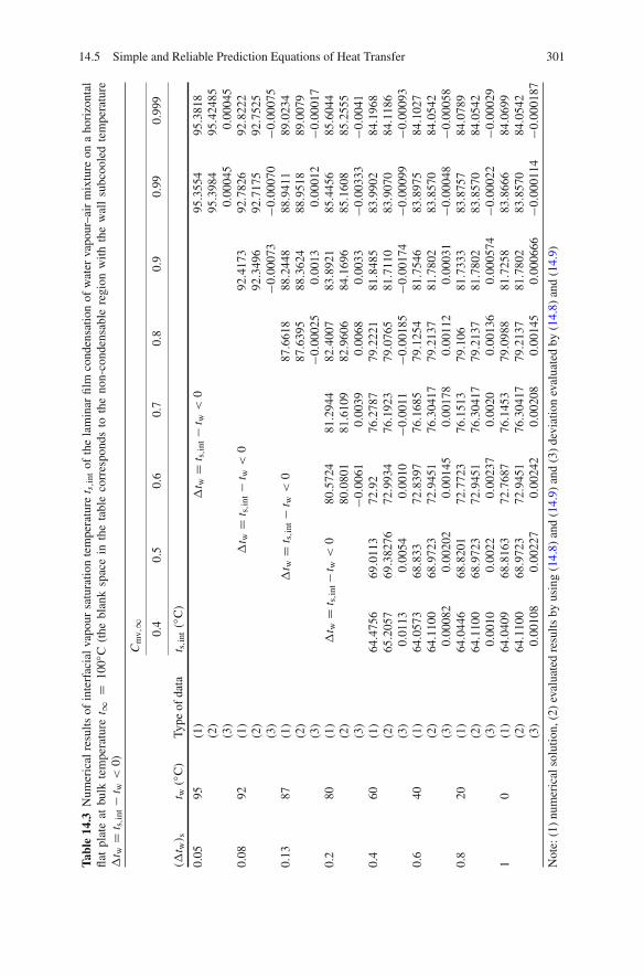
14.5 Simple and Reliable Prediction Equations of Heat Transfer 301
Tabl
e14
.3N
umer
ical
resu
ltsof
inte
rfac
ial
vapo
ursa
tura
tion
tem
pera
ture
t s,i
ntof
the
lam
inar
film
cond
ensa
tion
ofw
ater
vapo
ur–a
irm
ixtu
reon
aho
rizo
ntal
flat
plat
eat
bulk
tem
pera
ture
t ∞=
100◦
C(t
hebl
ank
spac
ein
the
tabl
eco
rres
pond
sto
the
non-
cond
ensa
ble
regi
onw
ithth
ew
all
subc
oole
dte
mpe
ratu
re�
t w=
t s,i
nt−
t w<
0)
Cm
v,∞
0.4
0.5
0.6
0.7
0.8
0.9
0.99
0.99
9
(�t w) s
t w(◦
C)
Type
ofda
tat s,i
nt(◦
C)
0.05
95(1
)�
t w=
t s,i
nt−
t w<
095.3
554
95.3
818
(2)
95.3
984
95.4
2485
(3)
0.00
045
0.00
045
0.08
92(1
)�
t w=
t s,i
nt−
t w<
092.4
173
92.7
826
92.8
222
(2)
92.3
496
92.7
175
92.7
525
(3)
−0.0
0073
−0.0
0070
−0.0
0075
0.13
87(1
)�
t w=
t s,i
nt−
t w<
087.6
618
88.2
448
88.9
411
89.0
234
(2)
87.6
395
88.3
624
88.9
518
89.0
079
(3)
−0.0
0025
0.00
130.
0001
2−0.0
0017
0.2
80(1
)�
t w=
t s,i
nt−t
w<
080.5
724
81.2
944
82.4
007
83.8
921
85.4
456
85.6
044
(2)
80.0
801
81.6
109
82.9
606
84.1
696
85.1
608
85.2
555
(3)
−0.0
061
0.00
390.
0068
0.00
33−0.0
0333
−0.0
041
0.4
60(1
)64.4
756
69.0
113
72.9
276.2
787
79.2
221
81.8
485
83.9
902
84.1
968
(2)
65.2
057
69.3
8276
72.9
934
76.1
923
79.0
765
81.7
110
83.9
070
84.1
186
(3)
0.01
130.
0054
0.00
10−0.0
011
−0.0
0185
−0.0
0174
−0.0
0099
−0.0
0093
0.6
40(1
)64.0
573
68.8
3372.8
397
76.1
685
79.1
254
81.7
546
83.8
975
84.1
027
(2)
64.1
100
68.9
723
72.9
451
76.3
0417
79.2
137
81.7
802
83.8
570
84.0
542
(3)
0.00
082
0.00
202
0.00
145
0.00
178
0.00
112
0.00
031
−0.0
0048
−0.0
0058
0.8
20(1
)64.0
446
68.8
201
72.7
723
76.1
513
79.1
0681.7
333
83.8
757
84.0
789
(2)
64.1
100
68.9
723
72.9
451
76.3
0417
79.2
137
81.7
802
83.8
570
84.0
542
(3)
0.00
100.
0022
0.00
237
0.00
200.
0013
60.
0005
74−0.0
0022
−0.0
0029
10
(1)
64.0
409
68.8
163
72.7
687
76.1
453
79.0
988
81.7
258
83.8
666
84.0
699
(2)
64.1
100
68.9
723
72.9
451
76.3
0417
79.2
137
81.7
802
83.8
570
84.0
542
(3)
0.00
108
0.00
227
0.00
242
0.00
208
0.00
145
0.00
0666
−0.0
0011
4−0.0
0018
7
Not
e:(1
)nu
mer
ical
solu
tion,
(2)
eval
uate
dre
sults
byus
ing
(14.
8)an
d(1
4.9)
and
(3)
devi
atio
nev
alua
ted
by(1
4.8)
and
(14.
9)

302 14 Heat and Mass Transfer on Laminar Forced Film Condensation
B = 2.8813
[(�tw)s
ts
]3
− 6.3245
[(�tw)s
ts
]2
+ 4.5528(�tw)s
ts− 1.6063
(0.2 ≤ (�tw)s
ts≤ 1
)
14.6 Condensate Mass Transfer Analysis
Consulting the mass transfer analysis of laminar forced film condensation of purevapour in Chap. 11, the related mass transfer analysis of laminar forced condensa-tion of vapour–gas mixture is given below.
The local mass flow rate gx entering the liquid film through the interface of liq-uid and vapour–gas mixture at position x corresponding to unit area of the plate isexpressed as
gx = ρl,s
(wxl,s
dδl
dx− wyl,s
)
s
With (12.17), (12.18), (12.20) and (12.21) for the assumed dimensionless coor-dinate variable ηlδ, local Reynolds number Rexl,s and dimensionless velocity com-ponents Wxl,s and Wyl,s of the liquid film, the above equation is changed to
gx = ρl,s
[wxm,∞Wxl,s
dδl
dx− wxm,∞
(1
2Rexl,s
)−1/2
Wyl,s
]
s
(14.12)
where
δl = ηlδ
(1
2
wxm,∞x
νl,s
)−1/2
x
dδl
dx= 1
2ηlδ
(1
2Rexl,s
)−1/2
(14.13)
Then,
gx = ρl,s
[wxm,∞Wxl,s
1
2ηlδ
(1
2Rexl,s
)−1/2
− wxv,∞(
1
2Rexl,s
)−1/2
Wyl,s
]
i.e.
gx = 1
2ρl,swxm,∞
(1
2Rexl,s
)−1/2 [ηlδWxl,s − 2Wyl,s
]
The above equation is rewritten as
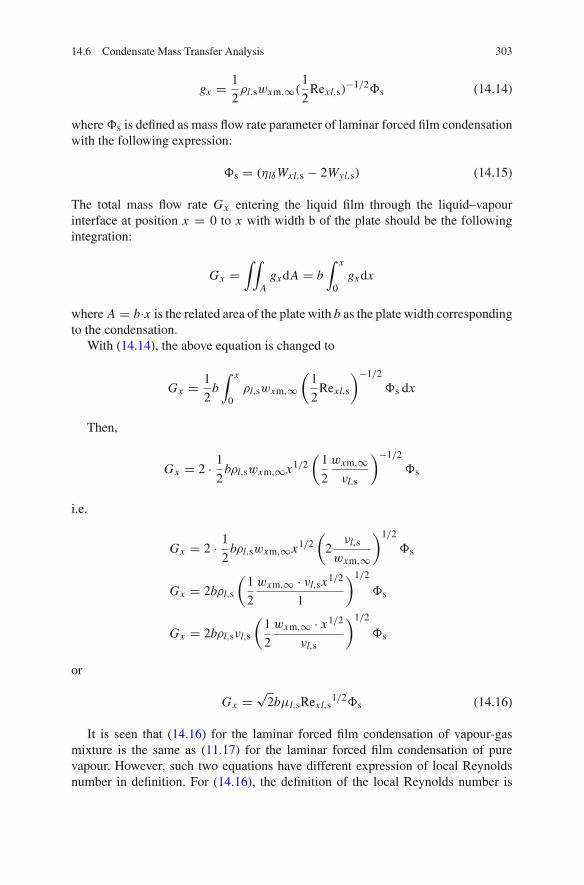
14.6 Condensate Mass Transfer Analysis 303
gx = 1
2ρl,swxm,∞(
1
2Rexl,s)
−1/2�s (14.14)
where�s is defined as mass flow rate parameter of laminar forced film condensationwith the following expression:
�s = (ηlδWxl,s − 2Wyl,s) (14.15)
The total mass flow rate Gx entering the liquid film through the liquid–vapourinterface at position x = 0 to x with width b of the plate should be the followingintegration:
Gx =∫∫
Agx dA = b
∫ x
0gx dx
where A = b·x is the related area of the plate with b as the plate width correspondingto the condensation.
With (14.14), the above equation is changed to
Gx = 1
2b∫ x
0ρl,swxm,∞
(1
2Rexl,s
)−1/2
�s dx
Then,
Gx = 2 · 1
2bρl,swxm,∞x1/2
(1
2
wxm,∞νl,s
)−1/2
�s
i.e.
Gx = 2 · 1
2bρl,swxm,∞x1/2
(2νl,s
wxm,∞
)1/2
�s
Gx = 2bρl,s
(1
2
wxm,∞ · νl,sx1/2
1
)1/2
�s
Gx = 2bρl,sνl,s
(1
2
wxm,∞ · x1/2
νl,s
)1/2
�s
or
Gx = √2bμl,sRexl,s
1/2�s (14.16)
It is seen that (14.16) for the laminar forced film condensation of vapour-gasmixture is the same as (11.17) for the laminar forced film condensation of purevapour. However, such two equations have different expression of local Reynoldsnumber in definition. For (14.16), the definition of the local Reynolds number is
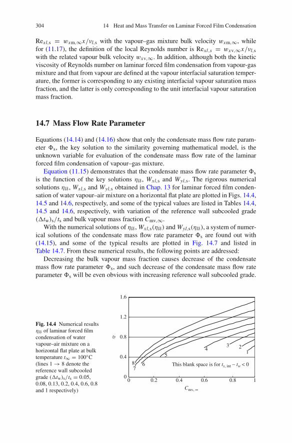
304 14 Heat and Mass Transfer on Laminar Forced Film Condensation
Rexl,s = wxm,∞x/νl,s with the vapour–gas mixture bulk velocity wxm,∞, whilefor (11.17), the definition of the local Reynolds number is Rexl,s = wxv,∞x/νl,swith the related vapour bulk velocity wxv,∞. In addition, although both the kineticviscosity of Reynolds number on laminar forced film condensation from vapour-gasmixture and that from vapour are defined at the vapour interfacial saturation temper-ature, the former is corresponding to any existing interfacial vapour saturation massfraction, and the latter is only corresponding to the unit interfacial vapour saturationmass fraction.
14.7 Mass Flow Rate Parameter
Equations (14.14) and (14.16) show that only the condensate mass flow rate param-eter �s, the key solution to the similarity governing mathematical model, is theunknown variable for evaluation of the condensate mass flow rate of the laminarforced film condensation of vapour–gas mixture.
Equation (11.15) demonstrates that the condensate mass flow rate parameter �sis the function of the key solutions ηlδ , Wxl,s and Wyl,s. The rigorous numericalsolutions ηlδ , Wxl,s and Wyl,s obtained in Chap. 13 for laminar forced film conden-sation of water vapour–air mixture on a horizontal flat plate are plotted in Figs. 14.4,14.5 and 14.6, respectively, and some of the typical values are listed in Tables 14.4,14.5 and 14.6, respectively, with variation of the reference wall subcooled grade(�tw)s/ts and bulk vapour mass fraction Cmv,∞.
With the numerical solutions of ηlδ , Wxl,s(ηlδ) and Wyl,s(ηlδ), a system of numer-ical solutions of the condensate mass flow rate parameter �s are found out with(14.15), and some of the typical results are plotted in Fig. 14.7 and listed inTable 14.7. From these numerical results, the following points are addressed:
Decreasing the bulk vapour mass fraction causes decrease of the condensatemass flow rate parameter �s, and such decrease of the condensate mass flow rateparameter �s will be even obvious with increasing reference wall subcooled grade.
Fig. 14.4 Numerical resultsηlδ of laminar forced filmcondensation of watervapour–air mixture on ahorizontal flat plate at bulktemperature t∞ = 100◦C(lines 1 → 8 denote thereference wall subcooledgrade (�tw)s/ts = 0.05,0.08, 0.13, 0.2, 0.4, 0.6, 0.8and 1 respectively)
0
0.4
0.8
1.2
1.6
0 0.2 0.4 0.6 0.8 1
η l
123
45
678
Cmv, ∞
This blank space is for ts, int − tw < 0

14.7 Mass Flow Rate Parameter 305
Fig. 14.5 Numerical resultsWyl,s(ηlδ) of laminar forcedfilm condensation of watervapour–air mixture on ahorizontal flat plate at bulktemperature t∞ = 100◦C(lines 1 → 5 denote thereference wall subcooledgrade (�tw)s/ts = 0.2, 0.4,0.6, 0.8 and 1 respectively)
0
0.005
0.01
0.015
0.02
0.025
0.03
0.035
0 0.2 0.4 0.6 0.8 11
8
Cmv,∞
Wyl
,s (
η lδ )
Fig. 14.6 Numerical resultsWxl,s(ηlδ) of laminar forcedfilm condensation of watervapour–air mixture on ahorizontal flat at bulktemperature t∞ = 100◦C(lines 1 → 8 denote thereference wall subcooledgrade (�tw)s/ts = 0.2, 0.4,0.6, 0.8 and 1 respectively)
0
0.04
0.08
0.12
0.16
0 0.2 0.4 0.6 0.8 11
8
Cmv,∞
Wxl
,s (
η lδ)
On the other hand, the condensate mass flow rate parameter �s will increase withincreasing reference wall subcooled grade.
The numerical solutions of the condensate mass flow rate parameter �s are for-mulated with (14.17) by means of a curve-fitting approach. The predicted results by(14.17) are also listed in Table 14.7, which are obviously coincident with the relatednumerical solutions.
�s = A ln
((�tw)s
ts
)+ B
(0.4 ≤ (�tw)s
ts≤ 1
)(14.17)
where
A = 0.0272(Cmv,∞
)−0.3865 (0.4 ≤ Cmv,∞ ≤ 0.999
)
B = −0.0112(Cmv,∞
)2 + 0.0215(Cmv,∞
)+ 0.0334(0.4 ≤ Cmv,∞ ≤ 0.999
)

306 14 Heat and Mass Transfer on Laminar Forced Film Condensation
Tabl
e14
.4N
umer
ical
resu
ltsη
lδof
lam
inar
forc
edfil
mco
nden
satio
nof
wat
erva
pour
–air
mix
ture
ona
hori
zont
alfla
tpla
teat
bulk
tem
pera
ture
t ∞=
100◦
C(t
hebl
ank
spac
ein
the
tabl
eco
rres
pond
sto
the
regi
onw
ithth
ew
alls
ubco
oled
tem
pera
ture�
t w=
t s,i
nt−
t w<
0)
Cm
v,∞
0.4
0.5
0.6
0.7
0.8
0.9
0.99
0.99
9
(�t w) s/
t st w
(◦C
)η
lδ
0.05
95�
t w=
t s,i
nt−
t w<
00.
612
0.62
550.
0892
�t w
=t s,i
nt−
t w<
00.
6203
0.74
490.
7555
0.13
87�
t w=
t s,i
nt−
t w<
00.
669
0.78
940.
879
0.88
760.
280
�t w
=t s,i
nt−
t w<
00.
5969
0.72
530.
8237
0.90
440.
968
0.97
450.
460
0.62
850.
7198
760.
8021
0.87
840.
9502
1.01
951.
0801
291.
0863
0.6
400.
717
0.81
396
0.90
260.
9834
1.06
0514
1.13
451.
1995
1.20
60.
820
0.81
926
0.92
435
1.01
951.
1078
1.19
111.
2712
1.34
141.
3483
61
00.
9399
1.05
471.
1585
1.25
455
1.34
521.
4321
91.
5085
1.51
6

14.7 Mass Flow Rate Parameter 307
Tabl
e14
.5N
umer
ical
resu
ltsW
yl,s(η
lδ)
ofla
min
arfo
rced
film
cond
ensa
tion
ofw
ater
vapo
ur–a
irm
ixtu
reon
aho
rizo
ntal
flat
plat
eat
bulk
tem
pera
ture
t ∞=
100◦
C(t
hebl
ank
spac
ein
the
tabl
eis
corr
espo
nds
toth
ere
gion
with
the
wal
lsub
cool
edte
mpe
ratu
re�
t w=
t s,i
nt−
t w<
0)
Cm
v,∞
0.4
0.5
0.6
0.7
0.8
0.9
0.99
0.99
9
(�t w) s/
t st w
(◦C
)W
yl,s(η
lδ)
0.05
95R
egio
nfo
r�
t w=
t s,i
nt−
t w<
00.
0002
90.
0003
050.
0892
Reg
ion
for�
t w=
t s,i
nt−
t w<
00.
0003
240.
0005
090.
0005
280.
1387
Reg
ion
for�
t w=
t s,i
nt−
t w<
00.
0004
490.
0007
220.
0010
220.
0010
560.
280
Reg
ion
for�
t w=
t s,i
nt−
t w<
00.
0003
950.
0007
430.
0012
370.
0018
710.
0025
090.
0025
710.
460
0.00
2309
0.00
4443
0.00
6158
0.00
7531
0.00
8658
0.00
9591
0.01
030.
0103
650.
640
0.01
1717
0.01
3608
0.01
5081
0.01
6196
0.01
7111
0.01
7849
0.01
8388
0.01
8436
0.8
200.
0208
640.
0225
240.
0237
720.
0247
330.
0254
820.
0260
570.
0264
550.
0264
881
00.
0300
240.
0315
180.
0326
10.
0334
220.
0340
230.
0344
540.
0347
190.
0347
4

308 14 Heat and Mass Transfer on Laminar Forced Film Condensation
Tabl
e14
.6N
umer
ical
resu
ltsW
xl,s(η
lδ)
ofla
min
arfo
rced
film
cond
ensa
tion
ofw
ater
vapo
ur–a
irm
ixtu
reon
aho
rizo
ntal
flat
plat
eat
bulk
tem
pera
ture
t ∞=
100◦
C(t
hebl
ank
spac
ein
the
tabl
eco
rres
pond
sto
the
regi
onw
ithth
ew
alls
ubco
oled
tem
pera
ture�
t w=
t s,i
nt−
t w<
0)
Cm
v,∞
0.4
0.5
0.6
0.7
0.8
0.9
0.99
0.99
9
(�t w) s/
t st w
(◦C
)W
xl,s(η
lδ)
0.05
95R
egio
nfo
r�
t w=
t s,i
nt−
t w<
00.
0018
960.
0019
510.
0892
Reg
ion
for�
t w=
t s,i
nt−
t w<
00.
0020
90.
0027
310.
0027
910.
1387
Reg
ion
for�
t w=
t s,i
nt−
t w<
00.
0026
80.
0036
510.
0046
360.
0047
450.
280
Reg
ion
for�
t w=
t s,i
nt−
t w<
00.
0026
410.
0040
890.
0059
790.
0082
20.
0102
690.
0104
520.
460
0.01
4547
0.02
420.
0298
70.
0331
480.
0350
430.
0360
230.
0363
850.
0363
970.
640
0.06
149
0.06
2318
0.06
183
0.06
0603
0.05
909
0.05
739
0.05
574
0.05
557
0.8
200.
0902
20.
0856
30.
0814
50.
0776
20.
0740
80.
0707
50.
0679
0.06
762
10
0.10
599
0.09
8552
0.09
241
0.08
715
0.08
250.
0782
90.
0747
60.
0744
2
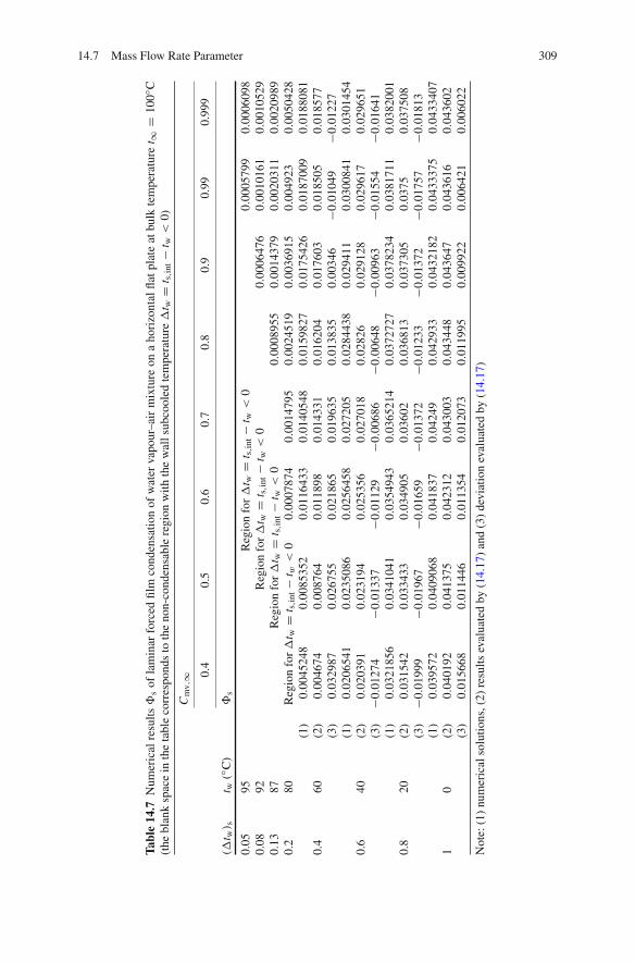
14.7 Mass Flow Rate Parameter 309
Tabl
e14
.7N
umer
ical
resu
lts�
sof
lam
inar
forc
edfil
mco
nden
satio
nof
wat
erva
pour
–air
mix
ture
ona
hori
zont
alfla
tpla
teat
bulk
tem
pera
ture
t ∞=
100◦
C(t
hebl
ank
spac
ein
the
tabl
eco
rres
pond
sto
the
non-
cond
ensa
ble
regi
onw
ithth
ew
alls
ubco
oled
tem
pera
ture�
t w=
t s,i
nt−
t w<
0)
Cm
v,∞ 0.
40.
50.
60.
70.
80.
90.
990.
999
(�t w) s
t w(◦
C)
�s
0.05
95R
egio
nfo
r�
t w=
t s,i
nt−
t w<
00.
0005
799
0.00
0609
80.
0892
Reg
ion
for�
t w=
t s,i
nt−
t w<
00.
0006
476
0.00
1016
10.
0010
529
0.13
87R
egio
nfo
r�
t w=
t s,i
nt−
t w<
00.
0008
955
0.00
1437
90.
0020
311
0.00
2098
90.
280
Reg
ion
for�
t w=
t s,i
nt−
t w<
00.
0007
874
0.00
1479
50.
0024
519
0.00
3691
50.
0049
230.
0050
428
0.4
60(1
)0.
0045
248
0.00
8535
20.
0116
433
0.01
4054
80.
0159
827
0.01
7542
60.
0187
009
0.01
8808
1(2
)0.
0046
740.
0087
640.
0118
980.
0143
310.
0162
040.
0176
030.
0185
050.
0185
77(3
)0.
0329
870.
0267
550.
0218
650.
0196
350.
0138
350.
0034
6−0.0
1049
−0.0
1227
0.6
40(1
)0.
0206
541
0.02
3508
60.
0256
458
0.02
7205
0.02
8443
80.
0294
110.
0300
841
0.03
0145
4(2
)0.
0203
910.
0231
940.
0253
560.
0270
180.
0282
60.
0291
280.
0296
170.
0296
51(3
)−0.0
1274
−0.0
1337
−0.0
1129
−0.0
0686
−0.0
0648
−0.0
0963
−0.0
1554
−0.0
1641
0.8
20(1
)0.
0321
856
0.03
4104
10.
0354
943
0.03
6521
40.
0372
727
0.03
7823
40.
0381
711
0.03
8200
1(2
)0.
0315
420.
0334
330.
0349
050.
0360
20.
0368
130.
0373
050.
0375
0.03
7508
(3)
−0.0
1999
−0.0
1967
−0.0
1659
−0.0
1372
−0.0
1233
−0.0
1372
−0.0
1757
−0.0
1813
10
(1)
0.03
9572
0.04
0906
80.
0418
370.
0424
90.
0429
330.
0432
182
0.04
3337
50.
0433
407
(2)
0.04
0192
0.04
1375
0.04
2312
0.04
3003
0.04
3448
0.04
3647
0.04
3616
0.04
3602
(3)
0.01
5668
0.01
1446
0.01
1354
0.01
2073
0.01
1995
0.00
9922
0.00
6421
0.00
6022
Not
e:(1
)nu
mer
ical
solu
tions
,(2)
resu
ltsev
alua
ted
by(1
4.17
)an
d(3
)de
viat
ion
eval
uate
dby
(14.
17)

310 14 Heat and Mass Transfer on Laminar Forced Film Condensation
14.8 Prediction Equations of Condensate Mass Transfer
In combination with the reliable formulated equation) for prediction of the con-densate mass flow rate parameter, the mass transfer theoretical expression (14.16)will become the following simple and reliable equation for prediction of condensatemass transfer of laminar forced condensation of saturated and superheated watervapour on the horizontal flat plate:
Gx = √2bμl,sRexl,s
1/2[
A ln
((�tw)s
ts
)+ B
] (0.4 ≤ (�tw)s
ts≤ 1
)
(14.18)where
A = 0.0272(Cmv,∞
)−0.3865 (0.4 ≤ Cmv,∞ ≤ 0.999
)
B = −0.0112(Cmv,∞
)2 + 0.0215(Cmv,∞
)+ 0.0334(0.4 ≤ Cmv,∞ ≤ 0.999
)
Obviously, the reliability of (14.18) is same as that of (14.17).
14.9 Equation of Interfacial Vapour Saturation Temperature
14.9.1 For Laminar Forced Film Condensationof Vapour–Gas Mixture
The prediction equation of interfacial vapour saturation temperature ts,int wasreported in Sect. 14.4 for the laminar forced film condensation of water vapour–airmixture. In this section, I will derive the dependent correlation of the interfacialvapour saturation temperature ts,int in order to investigate another way to predict theinterfacial vapour saturation temperature ts,int.
Consulting the condensate mass–energy transformation equation (11.32)with (11.33) for laminar forced film condensation of vapour, the present condensatemass–energy transformation equation for the laminar forced film condensation ofvapour–gas mixture becomes
(− dθl
dηl
)
ηl=0= Cmh�s (11.32)
with
Cmh = μl,shfg
λl,w(ts,int − tw
) (14.19)
Equation (14.19) describes the condensate mass–energy transformation coeffi-cient Cmh for laminar forced film condensation of vapour–gas mixture. Here, ts,int isthe interfacial vapour saturation temperature, λl,w is the liquid thermal conductivity

14.9 Equation of Interfacial Vapour Saturation Temperature 311
of the wall, μl,s and hfg are liquid absolute viscosity and latent heat at interfacialvapour saturation temperature ts,int, respectively.
Equation (14.19) is rewritten as
Cmhλl,w(ts,int − tw
)− μl,shfg = 0 (14.20)
where from (11.32) the condensate mass–energy transformation coefficient Cmh isdefined as
Cmh =
(− dθl(ηl)
dηl
)ηl=0
�s
Equation (14.20) is the equation for interfacial vapour saturation temperature oflaminar forced film condensation of vapour–gas mixture and describes the depen-dent relation of the interfacial vapour saturation temperature ts,int to the condensatemass–energy transformation coefficient Cmh, the liquid thermal conductivity of thewall temperature, λl,w, the liquid thermal conductivity of the wall, μl,s and hfg atinterfacial vapour saturation temperature ts,int.
14.9.2 For Laminar Forced Film Condensation of WaterVapour–Air Mixture
Based on the typical experimental data, the condensate latent hfg of water vapour atdifferent interfacial vapour saturation temperature, at an atmospheric pressure as thesystem pressure of the water vapour–air mixture, can be evaluated by the followingequation:
hfg = (−2.4355ts,int + 2503.2)× 103 (14.21)
According to (10.2) and (10.3), λl,w and μl,s are expressed as follows for water:
λl,w = −8.01 × 10⁻⁶tw2 + 1.94 × 10⁻³tw + 0.563 (14.22)
μl,s = exp
[−1.6 − 1150
ts,int + 273+(
690
ts,int + 273
)2]
× 10−3 (14.23)
Then, (14.20) is changed to
Cmh
(−8.01 × 10⁻⁶tw
2 + 1.94 × 10⁻³tw + 0.563) (
ts,int − tw)
− exp
[−1.6 − 1150
ts,int + 273+(
690
ts,int + 273
)2]
× (−2.4355ts,int + 2503.2)× 103 = 0 (14.24)

312 14 Heat and Mass Transfer on Laminar Forced Film Condensation
with the condensate mass-energy transformation coefficient, defined as
Cmh =
(− dθl(ηl)
dηl
)ηl=0
�s
Equation (14.24) is the alternative of the condensate mass–energy transformationequation for laminar forced film condensation of water vapour–air mixture, describ-ing the dependent relation of the interfacial vapour saturation temperature ts,int tothe condensate mass–energy transformation coefficient. While the latter depends onthe solutions, the wall dimensionless temperature gradient
(−dθl (ηl)
dηl
)
ηl=0
and condensate mass flow rate parameter �s . With the nonlinear algebraic equa-tion (14.24) for ts,int, the interfacial vapour saturation temperature ts,int can be easilyfound out with iteration approach for any given values of the wall dimensionlesstemperature gradient, condensate mass flow rate parameter, and interfacial vapoursaturation temperature. In fact, (14.24) can also be used for judgement of reliabilityof numerical solutions of the governing mathematical model.
14.10 Evaluation of Condensate Mass–Energy TransformationCoefficient
It is obvious that the condensate mass–energy transportation coefficient plays animportant role in the investigation of the transformation between the data of heatand mass transfer of the film condensation. In this section, the laminar forced filmcondensation of water vapour–air mixture on a horizontal flat plate at bulk tem-perature t∞ = 100◦C will be taken as an example to introduce the evaluation ofthe condensate mass–energy transportation coefficient. Here, I will introduce twoapproaches about such transformation.
The first approach to the evaluation of the condensate mass–energy transportationcoefficient is the numerical method. With the systems of key numerical solutions
(−dθl (ηl)
dηl
)
ηl=0
and �s listed in Figs. 14.1 and 14.7, respectively, the system of numerical solutionsof the condensate mass–energy transformation coefficient
Cmh =
(− dθl(ηl)
dηl
)ηl=0
�s

14.11 Summary 313
Fig. 14.7 Numerical results�s of laminar forced filmcondensation of watervapour–air mixture on ahorizontal flat plate at bulktemperature t∞ = 100◦C(lines 1 → 5 denote thereference wall subcooledgrade (�tw)s/ts = 0.2, 0.4,0.6, 0.8 and 1 respectively)
0
0.01
0.02
0.03
0.04
0.05
0 0.2 0.4 0.6 0.8 1
Φs
Cmν,∞1
8
is found out, and their typical values are listed in Table 14.8. On the other hand,for the evaluation of the condensate mass–energy transformation coefficient forlaminar forced film condensation of water vapour–air mixture, the formulated equa-tions (14.7) and (14.17) can also be applied for reliable evaluation of the dimension-less wall temperature gradient and the condensate mass flow rate parameter.
The second approach is to use the definition equation (14.19) to evaluate thecondensate mass–energy transformation coefficient. In this evaluation, the physi-cal property equations (14.21), (14.22) and (14.23) are used for determination ofthe related physical properties at the wall surface and the liquid–vapour interface,respectively. The listed numerical solutions of the interfacial vapour saturation tem-perature in Table 14.8 are taken from Table 14.3 for the laminar forced film con-densation of water vapour–air mixture on a horizontal flat plate at bulk temperaturet∞ = 100 ◦C. On this basis, a set of the evaluated results of condensate mass–energytransportation coefficient are evaluated with (14.19), and their typical values arelisted in Table 14.8.
It is seen from Table 14.8 that the results of the condensate mass–energy trans-formation coefficient evaluated by the two approaches are very well coincident. Itfollows that the condensate mass–energy transformation equation reported in thisbook is reliable.
According to the derivation, it is seen that the condensate mass–energy transfor-mation equation (11.32) with (11.33) is universally suitable for any laminar forcedfilm condensation. While, (14.19) is specialized for the laminar forced film conden-sation of vapour-gas mixture.
14.11 Summary
At present, it is the time to summarize the complete mathematical models of lam-inar forced film condensation of vapour–gas mixture in Table 14.9, including thetwo-phase film flows governing partial differential equations, similarity variables,dimensionless similarity governing equations, the physical property factor equa-tions, and heat and mass transfer equations.
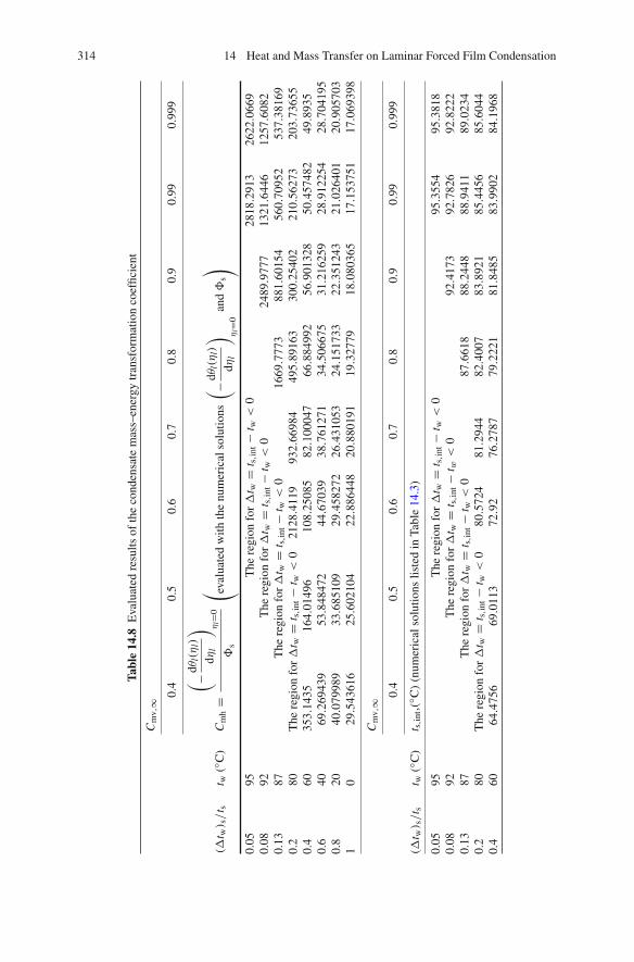
314 14 Heat and Mass Transfer on Laminar Forced Film Condensation
Tabl
e14
.8E
valu
ated
resu
ltsof
the
cond
ensa
tem
ass–
ener
gytr
ansf
orm
atio
nco
effic
ient
Cm
v,∞
0.4
0.5
0.6
0.7
0.8
0.9
0.99
0.99
9
(�t w) s/
t st w
(◦C
)C
mh
=
( −dθl(η
l)
dηl
) ηl=
0
�s
( eval
uate
dw
ithth
enu
mer
ical
solu
tions
( −dθl(η
l)
dηl
) ηl=
0an
d�
s)
0.05
95T
here
gion
for�
t w=
t s,i
nt−
t w<
028
18.2
913
2622.0
669
0.08
92T
here
gion
for�
t w=
t s,i
nt−
t w<
024
89.9
777
1321.6
446
1257.6
082
0.13
87T
here
gion
for�
t w=
t s,i
nt−
t w<
016
69.7
773
881.
6015
456
0.70
952
537.
3816
90.
280
The
regi
onfo
r�
t w=
t s,i
nt−
t w<
021
28.4
119
932.
6698
449
5.89
163
300.
2540
221
0.56
273
203.
7365
50.
460
353.
1435
164.
0149
610
8.25
085
82.1
0004
766.8
8499
256.9
0132
850.4
5748
249.8
935
0.6
4069.2
6943
953.8
4847
244.6
7039
38.7
6127
134.5
0667
531.2
1625
928.9
1225
428.7
0419
50.
820
40.0
7998
933.6
8510
929.4
5827
226.4
3105
324.1
5173
322.3
5124
321.0
2640
120.9
0570
31
029.5
4361
625.6
0210
422.8
8644
820.8
8019
119.3
2779
18.0
8036
517.1
5375
117.0
6939
8
(�t w) s/t s
t w(◦
C)
Cm
v,∞
0.4
0.5
0.6
0.7
0.8
0.9
0.99
0.99
9
t s,i
nt,(
◦ C)
(num
eric
also
lutio
nslis
ted
inTa
ble
14.3
)
0.05
95T
here
gion
for�
t w=
t s,i
nt−
t w<
095.3
554
95.3
818
0.08
92T
here
gion
for�
t w=
t s,i
nt−
t w<
092.4
173
92.7
826
92.8
222
0.13
87T
here
gion
for�
t w=
t s,i
nt−
t w<
087.6
618
88.2
448
88.9
411
89.0
234
0.2
80T
here
gion
for�
t w=
t s,i
nt−
t w<
080.5
724
81.2
944
82.4
007
83.8
921
85.4
456
85.6
044
0.4
6064.4
756
69.0
113
72.9
276.2
787
79.2
221
81.8
485
83.9
902
84.1
968

14.11 Summary 315
Tabl
e14
.8(c
ontin
ued)
Cm
v,∞
0.4
0.5
0.6
0.7
0.8
0.9
0.99
0.99
9
(�t w) s/
t st w
(◦C
)C
mh
=
( −dθl(η
l)
dηl
) ηl=
0
�s
( eval
uate
dw
ithth
enu
mer
ical
solu
tions
( −dθl(η
l)
dηl
) ηl=
0an
d�
s)
0.6
4064.0
573
68.8
3372.8
397
76.1
685
79.1
254
81.7
546
83.8
975
84.1
027
0.8
2064.0
446
68.8
201
72.7
723
76.1
513
79.1
0681.7
333
83.8
757
84.0
789
10
64.0
409
68.8
163
72.7
687
76.1
453
79.0
988
81.7
258
83.8
666
84.0
699
(�t w) s/t s
t w(◦
C)
Cm
v,∞
0.4
0.5
0.6
0.7
0.8
0.9
0.99
0.99
9
Cm
h=
μl,
shfg
λl,
w(t
s,in
t−
t w)
(eva
luat
edby
usin
g(1
4.19
)w
ith(1
4.21
),(1
4.22
)an
d(1
4.23
)an
dnu
mer
ical
solu
tions
oft s,i
ntlis
ted
inTa
ble
14.3
)
0.05
95T
here
gion
for�
t w=
t s,i
nt−
t w<
028
13.9
8726
18.6
060.
0892
The
regi
onfo
r�
t w=
t s,i
nt−
t w<
024
86.0
7113
19.8
5512
55.6
930.
1387
The
regi
onfo
r�
t w=
t s,i
nt−
t w<
016
67.8
4288
0.28
0255
9.65
4453
6.34
490.
280
The
regi
onfo
r�
t w=
t s,i
nt−
t w<
021
27.1
5693
1.63
0449
5.01
1529
9.43
5420
9.77
3420
3.41
640.
460
352.
3123
981
163.
2052
107.
4642
81.3
1813
66.1
3044
56.1
6829
49.7
3873
49.1
8226
0.6
4068.3
7116
888
52.9
9989
43.8
6424
37.9
8616
33.7
1271
30.4
9497
28.2
0271
27.9
9691
0.8
2039.1
7334
894
32.8
3423
28.6
552
25.6
6711
23.4
1056
21.6
3775
20.3
3266
20.2
1485
10
28.6
4684
007
24.7
6763
22.0
9596
20.1
2591
18.6
0122
17.3
7965
16.4
6712
16.3
8404

316 14 Heat and Mass Transfer on Laminar Forced Film Condensation
Table 14.9 Summary on complete mathematical models of laminar forced film condensation ofvapour–gas mixture
Governing partial differential equations for liquid film
Mass equation∂
∂x(ρlwxl)+ ∂
∂y
(ρlwyl
) = 0
Momentumequation
ρl
(wxl
∂wxl
∂x+ wyl
∂wxl
∂y
)= ∂
∂y
(μl∂wxl
∂y
)
Energy equation ρl
[wx∂(cpl t)
∂x+ wy
∂(cpl t)
∂y
]= ∂
∂y
(λl∂t
∂y
)
Governing partial differential equations for vapour-gas mixture film
Mass equation∂
∂x(ρmwxm)+ ∂
∂y
(ρmwym
) = 0
Momentumequation
ρm
(wxm
∂wxm
∂x+ wym
∂wxm
∂y
)= ∂
∂y
(μm
∂wxm
∂y
)
Energy equation ρm
[wxm
∂(cpm tm
)
∂x+ wym
∂(cpm tm
)
∂y
]= ∂
∂y
(λm∂tm∂y
)+
∂
∂y
[ρm Dv
(cpv − cpa
) ∂Cmv
∂ytm
]
Species equation∂ (wxmρmCmv)
∂x+ ∂(wymρmCmv
)
∂y= ∂
∂y
(Dvρm
∂Cmv
∂y
)
Boundary conditions of governing partial differential equations
y = 0 wxl = 0, wyl = 0, tl = twy = δl wxl,s = wxm,s
ρl,s
(wxl
∂δl
∂x− wyl
)
l,s= ρm,sCmv,s
(wxm
∂δm
∂x− wym
)
s= gx
μl,s
(∂wxl
∂y
)
s= μm,s
(∂wxm
∂y
)
s
λl,s
(∂Tl
∂y
)
sl
= λm,s
(∂Tm
∂y
)
s+ hfgρm,sCmv,s
(wxm
∂δm
∂x− wym
)
st = ts,intCmv = Cmv,s
ρm,sCm,vs
(wxm
∂δm
∂x− wym
)
s= Dvρm,s
(∂Cmv
∂y
)
sy → ∞ wxm = wxm,∞, tm = t∞,Cmv = Cmv,∞Similarity variables for liquid film
Dimensionlesscoordinatevariable ηl
ηl = y
x
(1
2Rexl,s
)1/2
Local Reynoldsnumber
Rexl,s = wxm,∞x
νl,s
Dimensionlesstemperature
θl (ηl) = tl − ts,int
tw − ts,int
Dimensionlessvelocitycomponents
wxl = wxm,∞Wxl (ηl)
Wxl (ηl) andWyl (ηl)
wyl = wxm,∞(
1
2Rexl,s
)−1/2
Wyl (ηl)

14.11 Summary 317
Table 14.9 (continued)
Similarity variables for vapour–gas mixture film
Dimensionlesscoordinatevariable
ηm = y
x
(1
2Rexm,∞
)1/2
Local Reynoldsnumber
Rexm,∞ = wxm,∞x
νm,∞
Dimensionlesstemperature
θm (ηm) = tm − t∞ts,int − t∞
Dimensionlessvelocitycomponents
wxm = wxm,∞Wxm (ηm)
Wxl (ηl) andWyl (ηl)
wym = wxm,∞(
1
2Rexm,∞
)−1/2Wym (ηm)
Vapour-relativemass fraction
�mv (ηm) = Cmv − Cmv,∞Cmv,s − Cmv,∞
Governing ordinary differential equations for liquid film
Mass equation −ηldWxl (ηl)
dηl+ 2
dWyl (ηl)
dηl+ 1
ρl
dρl
dηl
[−ηlWxl (ηl)+ 2Wyl (ηl)] = 0
Momentumequation
νl,s
νl
[−ηlWxl (ηl)+ 2(Wyl (ηl)
)] dWxl (ηl)
dηl= d2Wxl (ηl)
dη2l
+ 1
μl
dμl
dηl
dWxl (ηl)
dηl
Energy equation Prlνl,s
νl
{[−ηlWxl (ηl)+ 2Wyl (ηl)] dθl (ηl)
dηl+ [−ηlWxl (ηl)+ 2Wyl (ηl)
](θl (ηl)+ ts,int
tw − ts,int
)1
cpl
dcpl
dηl
}
= d2θl (ηl)
dη2l
+ 1
λl
∂λl
∂ηl
dθl (ηl)
dηl
Special
Governing ordinary differential equations for vapour–gas mixture film
Mass equation −ηmdWxm (ηm)
dηm+ 2
dWym (ηm)
dηm+ 1
ρm
dρm
dηm
[−ηm ·Wxm (ηm)+ 2Wym (ηm)]= 0
Momentumequation
νm,∞νm
[−ηm · Wxm (ηm)+ 2Wym (ηm)] dWxm (ηm)
dηm
= d2Wxm (ηm)
dη2m
+ 1
μm
dμm
dηl
dWxm (ηm)
dηm
Energy equation
νm,∞νm
{[−ηmWxm (ηm)+ 2Wym (ηm)] dθm (ηm)
dηm
+ [−ηmWxm (ηm)+ 2Wym (ηm)] 1
cpm
dcpm
dηm
(θm + t∞
ts,int − t∞
)}
= 1
Prm
[d2θm (ηm)
d2ηm+ 1
λm
dλm
dηm· dθm (ηm)
dηm
]
+ 1
Scm,∞νm,∞νm
cpv − cpg
cpm
(Cmv,s − Cmv,∞
) [d�m,v (ηm)
dηv
dθm (ηm)
dηm
+(θm + t∞
ts,int − t∞
)d2�mv (ηm)
dη2v
+(θm + t∞
ts,int − t∞
)1
ρm
dρm
dηl
d�mv (ηm)
dηv
]
Species equation[−ηmWxm (ηm)+ 2Wym (ηm)
] d�mv (ηm)
dηm
= 1
Scm,∞
[d2�mv (ηm)
dη2v
+ 1
ρm
dρm
dηm
d�mv (ηm)
dηm
]

318 14 Heat and Mass Transfer on Laminar Forced Film Condensation
Table 14.9 (continued)
Boundary conditions of governing ordinary differential equationsηl = 0 : Wxl = 0, Wyl = 0, θl = 1ηl = ηlδ Wxm,∞ (ηm) = Wxl,s (ηl)
Wym,s (ηm) = 1
2Cmv,s
ρl,s
ρm,s
(νl,s
νm,∞
)1/2 [−ηlδ · Wxl,s (ηl)+ 2Wyl,s (ηl)]
(dWxm (ηm)
dηm
)
s= μl,s
μm,s
(νm,∞νl,s
)1/2 ( dWx (ηl)
dηll
)
s(dθm (ηm)
dηm
)
s=
λl,s
(νm,∞νl,s
)1/2 (tw − ts,int
) (dθl (ηl)
dηl
)
s+ 2hfgρm,sνm,∞Cmv,sWym,s (ηm)
λm,s(ts,int − t∞
)θl,s (ηlδ) = 0, θm,s (ηm0) = 1�mv,s (ηm0) = 1, Cmv = Cmv,s(
d�mv (ηm)
dηm
)
s= −2Scm,∞
Cmv,s
Cmv,s − Cmv,∞Wym,s (ηm0)
ηm → ∞ Wxm,∞ (ηm∞) = 1, θm,∞ = 0, �mv,∞ = 0
Physical property factor equations of condensate liquid film
For condensatewater filmmedium
Prl = μl · cpl
λl=
[exp
(−1.6 − 1150
T+(
690
T
)2)
× 10−3
]× 4200
−8.01 × 10⁻⁶t2 + 1.94 × 10⁻³t + 0.5631
cpl
dcpl
dηl= 0
1
ρl
dρl
dηl=
[−2 × 4.48 × 10−3t (tw − ts)
dθl (ηl)
dηl
]
(−4.48 × 10⁻³t2 + 999.9)
1
λl
dλl
dηl=
[(−2 × 8.01 × 10−6 + 1.94 × 10⁻³
)(tw − ts)
dθl (ηl)
dηl
]
−8.01 × 10⁻⁶t2 + 1.94 × 10⁻³t + 0.563
1
μl
dμl
dηl=(
1150
T 2− 2 × 6902
T 3
)(tw − ts)
dθl (ηl)
dηl
Physical property factor equations of vapour–gas mixture film
Concentration-dependentphysicalpropertyfactors
1
ρm
dρm
dηm= 1
ρg
dρg
dηm+ 1
ρv
dρv
dηm− Cmv
(ρv − ρg
)
(1 − Cmv) ρv + Cmvρg[(1 − Cmv)
Cmv
ρv(ρv − ρg
) 1
ρv
dρv
dηm+ ρg(
ρv − ρg) 1
ρg
dρg
dηm
− Cmv,s − Cmv,∞Cmv
d�mv (ηm)
dηm
]
1
μm
dμm
dηm= Cmv
μv
μm
1
μv
dμv
dηm+ (1 − Cmv)
μg
μm
1
μg
dμg
dηm
+ μv − μg
μm
(Cmv,s − Cmv,∞
) d�mv
dηm1
λm
dλm
dηm= Cmv
λv
λm
1
λv
dλv
dηm+ (1 − Cm,v
) λg
λm
1
λg
dλg
dηm
+ λv − λg
λm
(Cmv,s − Cmv,∞
) d�mv
dηm

14.11 Summary 319
Table 14.9 (continued)
Temperaturedependentphysical propertyfactors
For density factors1
ρv
dρv
dηm= −(Ts,int/T∞ − 1
)dθm/dηm(
Ts,int/T∞ − 1)θm + 1
,
1
ρg
dρg
dηm= −(Ts,int/T∞ − 1
)dθm/dηm(
Ts,int/T∞ − 1)θm+1
For absolute viscosity factors
1
μv
dμv
dηm= nμ,v
(Ts,int/T∞ − 1
)dθm/dηm(
Ts,int/T∞ − 1)θm + 1
,
1
μg
dμg
dηm= nμ,g
(Ts,int/T∞ − 1
)dθm/dηm(
Ts,int/T∞ − 1)θm + 1
For thermal conductivity factors
1
λv
dλv
dηm= nλ,v
(Ts,int/T∞ − 1
)dθm/dηm(
Ts,int/T∞ − 1)θm + 1
,
1
λg
dλg
dηm= nλ,g
(Ts,int/T∞ − 1
)dθm/dηm(
Ts,int/T∞ − 1)θm + 1
Condensate heat transfer
Wall dimensionlesstemperature grade
For laminar forced film condensation of water vapour–air mixture on ahorizontal plate at t∞ = 100◦C
−(
dθl
dηl
)
ηl=0= ACmv,∞ B
(0.4 ≤ Cmv,∞ ≤ 0.999
where
A = 0.5868
[(�tw)s
ts
]−0.3272
(0.05 ≤ (�tw)s
ts≤ 0.2
)
A = −0.334(�tw)s
ts+ 1.0766
(0.2 ≤ (�tw)s
ts≤ 1
)
B = −0.2486
[(�tw)s
ts
]−0.8082
(0.05 ≤ (�tw)s
ts≤ 0.2
)
B = 2.8813
[(�tw)s
ts
]3
− 6.3245
[(�tw)s
ts
]2
+ 4.5528(�tw)s
ts− 1.6063
(0.2 ≤ (�tw)s
ts≤ 1
)
Local values of heattransfer,
Nuxl,w = αx,wx
λl,w
qx,w = λl,w(tw − ts,int
) (1
2Rex l,s
)1/2
x−1(
−dθl (ηl)
dηl
)
ηl=0
αx,w = λl,w
(1
2Rex l,s
)1/2
x−1(
−dθl (ηl)
dηl
)
ηl=0
Nuxl,w =(
1
2Rexl,s
)1/2 (−dθl (ηl)
dηl
)
ηl=0
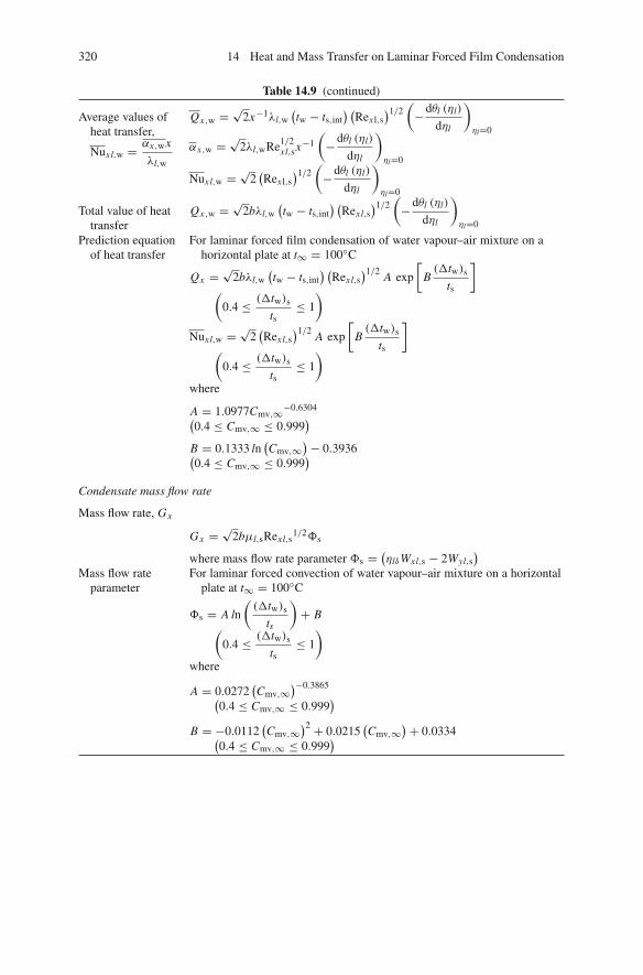
320 14 Heat and Mass Transfer on Laminar Forced Film Condensation
Table 14.9 (continued)
Average values ofheat transfer,
Nuxl,w = αx,wx
λl,w
Qx,w = √2x−1λl,w
(tw − ts,int
) (Rex l,s
)1/2 (−dθl (ηl)
dηl
)
ηl=0
αx,w = √2λl,wRe1/2
xl,sx−1(
−dθl (ηl)
dηl
)
ηl=0
Nuxl,w = √2(Rex l,s
)1/2 (−dθl (ηl)
dηl
)
ηl=0
Total value of heattransfer
Qx,w = √2bλl,w
(tw − ts,int
) (Rexl,s
)1/2 (−dθl (ηl)
dηl
)
ηl=0
Prediction equationof heat transfer
For laminar forced film condensation of water vapour–air mixture on ahorizontal plate at t∞ = 100◦C
Qx = √2bλl,w
(tw − ts,int
) (Rexl,s
)1/2A exp
[B(�tw)s
ts
]
(0.4 ≤ (�tw)s
ts≤ 1
)
Nuxl,w = √2(Rexl,s
)1/2A exp
[B(�tw)s
ts
]
(0.4 ≤ (�tw)s
ts≤ 1
)
where
A = 1.0977Cmv,∞−0.6304(0.4 ≤ Cmv,∞ ≤ 0.999
)
B = 0.1333 ln(Cmv,∞
)− 0.3936(0.4 ≤ Cmv,∞ ≤ 0.999
)
Condensate mass flow rate
Mass flow rate, Gx
Gx = √2bμl,sRexl,s
1/2�s
where mass flow rate parameter �s = (ηlδWxl,s − 2Wyl,s)
Mass flow rateparameter
For laminar forced convection of water vapour–air mixture on a horizontalplate at t∞ = 100◦C
�s = A ln
((�tw)s
ts
)+ B
(0.4 ≤ (�tw)s
ts≤ 1
)
where
A = 0.0272(Cmv,∞
)−0.3865(0.4 ≤ Cmv,∞ ≤ 0.999
)
B = −0.0112(Cmv,∞
)2 + 0.0215(Cmv,∞
)+ 0.0334(0.4 ≤ Cmv,∞ ≤ 0.999
)
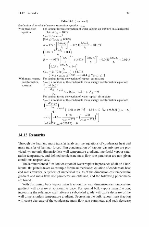
14.12 Remarks 321
Table 14.9 (continued)
Evaluation of interfacial vapour saturation equations ts,intWith prediction
equationFor laminar forced convection of water vapour–air mixture on a horizontal
plate at t∞ = 100◦Cts,int = ACmv,∞ B(0.4 ≤ Cmv,∞ ≤ 0.999
)
A = 177.5
[(�tw)s
ts
]2
− 112.12(�tw)s
ts+ 100.59
(0.05 ≤ (�tw)s
ts≤ 0.4
)
B = −4.9374
[(�tw)s
ts
]3
+ 3.6734
[(�tw)s
ts
]2
− 0.0445(�tw)s
ts+ 0.0243
(0.05 ≤ (�tw)s
ts≤ 0.4
)
ts,int = 21.79 ln(Cmv,∞
)+ 84.076(0.4 ≤ Cmv,∞ ≤ 0.999
)and(0.4 ≤ Cmv,∞ ≤ 1
)With mass–energy
transformationequation
For laminar forced convection of vapour–gas mixturets,int is a solution of the condensate mass–energy transformation equation:(
−dθl (ηl)
dηl
)
ηl=0
�sλl,w(ts,int − tw
)− μl,shfg = 0
For laminar forced convection of water vapour–air mixturets,int is a solution of the condensate mass–energy transformation equation:(
−dθl (ηl)
dηl
)
ηl =0
�s
(−8.01 × 10⁻⁶t2w + 1.94 × 10⁻³tw + 0.563
) (ts,int − tw
)
− exp
[−1.6 − 1150
ts,int + 273+(
690
ts,int + 273
)2]
(−2.4355ts,int + 2503.2) = 0
14.12 Remarks
Through the heat and mass transfer analyses, the equations of condensate heat andmass transfer of laminar forced film condensation of vapour–gas mixture are pro-vided, where only dimensionless wall temperature gradient, interfacial vapour satu-ration temperature, and defined condensate mass flow rate parameter are non-givenconditions respectively.
The laminar forced film condensation of water vapour in presence of air on a hor-izontal flat plate is taken as example for the numerical calculation of condensate heatand mass transfer. A system of numerical results of the dimensionless temperaturegradient and mass flow rate parameter are obtained, and the following phenomenaare found.
With decreasing bulk vapour mass fraction, the wall dimensionless temperaturegradient will increase at accelerative pace. For special bulk vapour mass fraction,increasing the reference wall reference subcooled grade will cause decrease of thewall dimensionless temperature gradient. Decreasing the bulk vapour mass fractionwill cause decrease of the condensate mass flow rate parameter, and such decrease
322 14 Heat and Mass Transfer on Laminar Forced Film Condensation
of the mass flow rate parameter will be even obvious with increasing wall subcooledgrade. For a special bulk vapour mass fraction, increasing the reference wall sub-cooled grade will cause increase of the condensate mass flow rate parameter. Thesephenomena demonstrate decisive effect of the non-condensable gas on condensateheat and mass transfer of the laminar forced film condensation of vapour–gas mix-ture.
The system of the rigorous key solutions of the wall dimensionless temperaturegradient and the condensate mass flow rate parameter is formulated the simple andreliable equations for the laminar film condensation of water vapour–air mixture. Incombination with the provided theoretical heat and transfer equations, these formu-lated equations of the wall dimensionless temperature gradient and condensate massflow rate parameter can be used for simple and reliable evaluation of the heat andmass transfer of laminar film condensation of water vapour–air mixture.
The interfacial vapour saturation temperature necessary for correct predictionof laminar film condensation of vapour–gas mixture is deeply investigated here.By taking the laminar forced film condensation of water vapour–air mixture as anexample, three methods are reported for evaluation of the interfacial vapour satu-ration temperature: (1) the numerical calculation method, (2) prediction with therelated formulation equation and (3) prediction by solving the modified condensatemass–energy transformation equation for describing the dependent relation for theinterfacial vapour saturation temperature. The calculated results of the interfacialvapour saturation temperature related to the different methods are well coincident.It proves that the system of investigations in this chapter on similarity analysismethod, the similarity mathematical model, the numerical calculation and treatmentmethod of temperature- and concentration- dependent physical properties is validfor extensive study of heat and mass transfer of laminar forced film condensation ofvapour–gas mixture.
The author believes that the analysis and calculation methods reported in thiswork can be conveniently extended to other different types of laminar forced filmcondensation from vapour–gas mixture.
14.13 Calculation Examples
Example 1 A flat plate, 0.3 m in width and 0.3 m in length, is located horizontally inthe flowing water vapour–air mixture with 2.9 m/s as the bulk flow velocity. The walltemperature is tw = 85 ◦C, reference vapour saturation temperature is ts = 100◦C,the vapour bulk temperature is t∞ = 100◦C and the bulk vapour mass fraction isCm,v∞ = 0.95. Please solve following questions:
(1) Calculate heat transfer rate on the plate.(2) From the heat transfer rate obtained in solution (1) for laminar forced film con-
densation of water vapour–air mixture on the horizontal flat plate and the cor-responding result of pure vapour calculated in Example 1 of Chap. 11, whichpoint can you get?
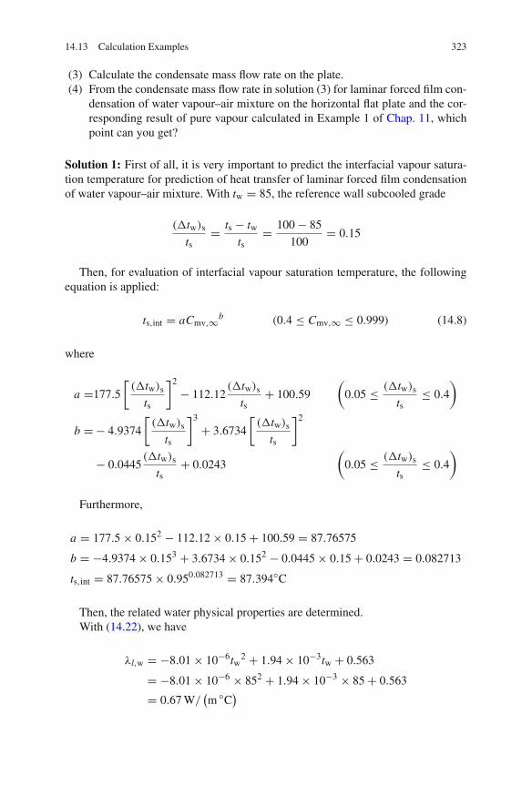
14.13 Calculation Examples 323
(3) Calculate the condensate mass flow rate on the plate.(4) From the condensate mass flow rate in solution (3) for laminar forced film con-
densation of water vapour–air mixture on the horizontal flat plate and the cor-responding result of pure vapour calculated in Example 1 of Chap. 11, whichpoint can you get?
Solution 1: First of all, it is very important to predict the interfacial vapour satura-tion temperature for prediction of heat transfer of laminar forced film condensationof water vapour–air mixture. With tw = 85, the reference wall subcooled grade
(�tw)sts
= ts − twts
= 100 − 85
100= 0.15
Then, for evaluation of interfacial vapour saturation temperature, the followingequation is applied:
ts,int = aCmv,∞b (0.4 ≤ Cmv,∞ ≤ 0.999) (14.8)
where
a =177.5
[(�tw)s
ts
]2
− 112.12(�tw)s
ts+ 100.59
(0.05 ≤ (�tw)s
ts≤ 0.4
)
b = − 4.9374
[(�tw)s
ts
]3
+ 3.6734
[(�tw)s
ts
]2
− 0.0445(�tw)s
ts+ 0.0243
(0.05 ≤ (�tw)s
ts≤ 0.4
)
Furthermore,
a = 177.5 × 0.152 − 112.12 × 0.15 + 100.59 = 87.76575
b = −4.9374 × 0.153 + 3.6734 × 0.152 − 0.0445 × 0.15 + 0.0243 = 0.082713
ts,int = 87.76575 × 0.950.082713 = 87.394◦C
Then, the related water physical properties are determined.With (14.22), we have
λl,w = −8.01 × 10⁻⁶tw2 + 1.94 × 10⁻³tw + 0.563
= −8.01 × 10−6 × 852 + 1.94 × 10−3 × 85 + 0.563
= 0.67 W/(m ◦C)
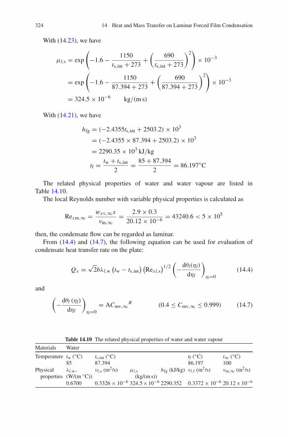
324 14 Heat and Mass Transfer on Laminar Forced Film Condensation
With (14.23), we have
μl,s = exp
(−1.6 − 1150
ts,int + 273+
(690
ts,int + 273
)2)
× 10−3
= exp
(−1.6 − 1150
87.394 + 273+
(690
87.394 + 273
)2)
× 10−3
= 324.5 × 10⁻⁶ kg/(m s)
With (14.21), we have
hfg = (−2.4355ts,int + 2503.2)× 103
= (−2.4355 × 87.394 + 2503.2)× 103
= 2290.35 × 103 kJ/kg
tf = tw + ts,int
2= 85 + 87.394
2= 86.197◦C
The related physical properties of water and water vapour are listed inTable 14.10.
The local Reynolds number with variable physical properties is calculated as
Rexm,∞ = wxv,∞x
νm,∞= 2.9 × 0.3
20.12 × 10−6= 43240.6 < 5 × 10⁵
then, the condensate flow can be regarded as laminar.From (14.4) and (14.7), the following equation can be used for evaluation of
condensate heat transfer rate on the plate:
Qx = √2bλl,w
(tw − ts,int
) (Rexl,s
)1/2(
−dθl(ηl)
dηl
)
ηl=0(14.4)
and(
−dθl (ηl)
dηl
)
ηl=0= ACmv,∞B (0.4 ≤ Cmv,∞ ≤ 0.999) (14.7)
Table 14.10 The related physical properties of water and water vapour
Materials Water
Temperature tw (◦C) ts,int (◦C) tf (◦C) t∞ (◦C)85 87.394 86.197 100
Physicalproperties
λl,w,(W/(m ◦C))
νl,s (m2/s) μl,s(kg/(m s))
hfg (kJ/kg) νl,f (m2/s) νm,∞ (m2/s)
0.6700 0.3326 × 10⁻⁶ 324.5×10⁻⁶ 2290.352 0.3372 × 10⁻⁶ 20.12×10⁻⁶

14.13 Calculation Examples 325
With (�tw)sts
= 0.15 we have
A = 0.5868
((�tw)s
ts
)−0.3272 (0.05 ≤ (�tw)s
ts≤ 0.2
)
B = −0.2486
((�tw)s
ts
)−0.8082 (0.05 ≤ (�tw)s
ts≤ 0.2
)
Here,
A = 0.5868 × (0.15)−0.3272 = 1.09162
B = −0.2486 × (0.15)−0.8082 = −1.15182(−dθl (ηl)
dηl
)
ηl=0= 1.09162 × 0.95−1.15182 = 1.158057
Rexl,s = wxm,∞x
νl,s= 2.9 × 0.3
0.3326 × 106= 2615754.7
Thus, the heat transfer rate on the plate is calculated as
Qx = √2 × 0.3 × 0.67 × (85 − 87.394)× 2615754.71/2 × 1.158057
= −1274.6 W
where the negative value of the result of heat transfer rate shows that the heat flux isfrom the vapour–gas mixture bulk to the wall plate surface.
Here, it should be indicated that the wall subcooled temperature of this exampleis only equal to
ts,int − tw = 87.394 − 85 = 2.394◦C
so small wall subcooled temperature requires a very accurate determination of theinterfacial vapour saturation temperature. Otherwise, a big deviation for the wallsubcooled temperature ts,int − tw will be easily produced, which will cause a bigdeviation for the calculated result of the heat transfer of the laminar forced filmcondensation of vapour–gas mixture.
Solution 2: If we take (Qx )m and (Qx )p as heat transfer rates for laminar film con-densation from water vapour–air mixture and pure water vapour, respectively, theirratio will be
(Qx )m
(Qx )p= 1274.6
5225.4= 0.2439
where (Qx )p = 5225.4 comes from the calculated result of example 1 of Chap. 11.The very small ratio (Qx )m/(Qx )p demonstrates that the non-condensable air in thevapour–gas mixture strongly reduces the condensate heat transfer.
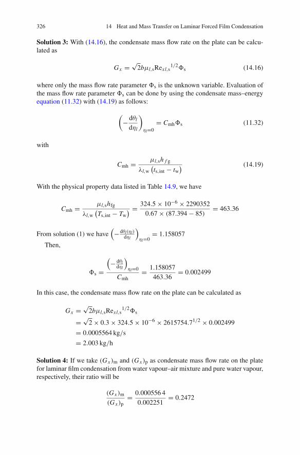
326 14 Heat and Mass Transfer on Laminar Forced Film Condensation
Solution 3: With (14.16), the condensate mass flow rate on the plate can be calcu-lated as
Gx = √2bμl,sRexl,s
1/2�s (14.16)
where only the mass flow rate parameter �s is the unknown variable. Evaluation ofthe mass flow rate parameter �s can be done by using the condensate mass–energyequation (11.32) with (14.19) as follows:
(− dθl
dηl
)
ηl=0= Cmh�s (11.32)
with
Cmh = μl,sh f g
λl,w(ts,int − tw
) (14.19)
With the physical property data listed in Table 14.9, we have
Cmh = μl,shfg
λl,w(Ts,int − Tw
) = 324.5 × 10−6 × 2290352
0.67 × (87.394 − 85)= 463.36
From solution (1) we have(−dθl(ηl)
dηl
)ηl=0
= 1.158057
Then,
�s =
(− dθl
dηl
)ηl=0
Cmh= 1.158057
463.36= 0.002499
In this case, the condensate mass flow rate on the plate can be calculated as
Gx = √2bμl,sRexl,s
1/2�s
= √2 × 0.3 × 324.5 × 10−6 × 2615754.71/2 × 0.002499
= 0.0005564 kg/s
= 2.003 kg/h
Solution 4: If we take (Gx )m and (Gx )p as condensate mass flow rate on the platefor laminar film condensation from water vapour–air mixture and pure water vapour,respectively, their ratio will be
(Gx )m
(Gx )p= 0.000556 4
0.002251= 0.2472

Exercises 327
where (Gx )p = 0.002251 comes from the calculated result of example 1 ofChap. 11. The very small ratio (Gx )m/(Gx )p demonstrates that the non-condensableair in the vapour–gas mixture strongly reduces the condensate mass transfer. On theother hand, it is seen that the evaluated ratio (Gx )m/(Gx )p is very close to the eval-uated ratio (Qx )m/(Qx )p, which demonstrates that the related theoretical analysisand calculation methods are reliable.
Exercises
1. Please point out at least two approaches to evaluate the interfacial vapour satura-tion temperature ts,int.
2. Follow example 1, in which only the wall temperature is changed to 65◦C andall other conditions are kept. Please solve following questions:
(1) Calculate heat transfer rate on the plate.(2) From the heat transfer rate obtained in solution (1) for laminar forced film
condensation of water vapour–air mixture on the horizontal flat plate and thecorresponding result of pure vapour calculated in exercise 2 of Chap. 11,which point can you get?
(3) Calculate the condensate mass flow rate on the plate.(4) From the condensate mass flow rate in solution (3) for laminar forced film
condensation of water vapour–air mixture on the horizontal flat plate and thecorresponding result of pure vapour calculated in example 1 of Chap. 11,which point can you get?
3. Please explain why the condensate mass–energy transformation equation(
− dθl
dηl
)
ηl=0= Cmh�s (11.32)
is universally eligible for laminar forced film condensation of both pure vapourand vapour–gas mixture.
4. The following two equations describe the condensate mass–energy transforma-tion coefficient, respectively, for laminar forced film condensation of vapour andthat of vapour–gas mixture:
Cmh = μl,shfg
λl,w (ts − tw)(11.33)
Cmh = μl,shfg
λl,w(ts,int − tw
) (14.19)
(1) Please identify the related physical significances of the physical propertyvariables μl,s, hfg and λl,w in the two equations.
(2) Explain the coincidence of the two equations and analyze the physical sig-nificance of the condensate mass–energy transformation equation.


Part IVAppendix


Appendix ATables with Physical Properties
Physical Properties of Gases at Atmospheric Pressure
Air [1]
T K ρ kg/m3cpkJ/(kg ◦C)
μ× 106
kg/(m s)ν × 106
m2/sλ
W/(m ◦C)a × 106
m2/s Pr
100 3.5562 1.032 7.11 1.999 0.00934 2.54 0.786150 2.3364 1.012 10.34 4.426 0.0138 5.84 0.758200 1.7458 1.007 13.25 7.59 0.0181 10.3 0.737250 1.3947 1.006 15.96 11.443 0.0223 15.9 0.720300 1.1614 1.007 18.46 15.895 0.0263 22.5 0.707350 0.9950 1.009 20.82 20.925 0.0300 29.9 0.7400 0.8711 1.014 23.01 26.415 0.0338 38.3 0.69450 0.7740 1.021 25.07 32.39 0.0373 47.2 0.686500 0.6964 1.030 27.01 38.785 0.0407 56.7 0.684550 0.6329 1.040 28.84 45.568 0.0439 66.7 0.683600 0.5804 1.051 30.58 52.688 0.0469 76.9 0.685650 0.5356 1.063 32.25 60.213 0.0497 87.3 0.69700 0.4975 1.075 33.88 68.101 0.05240 98 0.695750 0.4643 1.087 35.46 76.373 0.0549 109 0.702800 0.4354 1.099 36.98 84.933 0.0573 120 0.709850 0.4097 1.11 38.43 93.8 0.0596 131 0.716900 0.3868 1.121 39.81 102.921 0.0620 143 0.720950 0.3666 1.131 41.13 112.193 0.0643 155 0.723
1000 0.3482 1.141 42.44 121.884 0.0667 168 0.7261100 0.3166 1.159 44.9 141.819 0.0715 195 0.7281200 0.2920 1.175 47.3 161.986 0.0763 224 0.728
D.Y. Shang, Theory of Heat Transfer with Forced Convection Film Flows,Heat and Mass Transfer, DOI 10.1007/978-3-642-12581-2_15,C© Springer-Verlag Berlin Heidelberg 2011
331

332 Appendix A Tables with Physical Properties
Monoxide, CO [1]
T K ρ kg/m3cpkJ/(kg ◦C)
μ× 106
kg/(m s)ν × 106
m2/sλ
W/(m ◦C)a × 106
m2/s Pr
200 1.6888 1.045 12.7 7.5201 0.017 9.63 0.781220 1.5341 1.044 13.7 8.9303 0.0190 11.9 0.753240 1.4055 1.043 14.7 10.4589 0.0206 14.1 0.744260 1.2967 1.043 15.7 12.1077 0.0221 16.3 0.741280 1.2038 1.042 16.6 13.7897 0.0236 18.8 0.733300 1.1233 1.043 17.5 15.5791 0.025 21.3 0.730320 1.0529 1.043 18.4 17.4755 0.0263 23.9 0.730340 0.9909 1.044 19.3 19.4772 0.0278 26.9 0.725360 0.9357 1.045 20.2 21.5881 0.0291 29.8 0.729380 0.8864 1.047 21 23.6913 0.0305 32.9 0.719400 0.8421 1.049 21.8 25.8877 0.0318 36.0 0.719450 0.7483 1.055 23.7 31.6718 0.0350 44.3 0.714500 0.67352 1.065 25.4 37.7123 0.0381 53.1 0.710550 0.61226 1.076 27.1 44.2622 0.0411 62.4 0.710600 0.56126 1.088 28.6 50.9568 0.0440 72.1 0.707650 0.51806 1.101 30.1 58.1014 0.0470 82.4 0.705700 0.48102 1.114 31.5 65.4858 0.0500 93.3 0.702750 0.44899 1.127 32.9 73.2756 0.0528 104 0.702800 0.42095 1.140 34.3 81.4824 0.0555 116 0.705
Helium, He [1]
T K ρ kg/m3cpkJ/(kg ◦C)
μ× 106
kg/(m s)ν × 106
m2/sλ
W/(m ◦C)A × 106
m2/s Pr
100 0.4871 5.193 9.63 19.77 0.073 28.9 0.686120 0.406 5.193 10.7 26.36 0.0819 38.8 0.679140 0.3481 5.193 11.8 33.90 0.0907 50.2 0.676160 0.30945 5.193 12.9 41.69 0.0992 63.2 0.6745180 0.2708 5.193 13.9 51.33 0.1072 76.2 0.673200 0.2462 5.193 15 60.93 0.1151 91.6 0.674220 0.2216 5.193 16 72.20 0.1231 107 0.675240 0.20455 5.193 17 83.11 0.13 124 0.6785260 0.1875 5.193 18 96 0.137 141 0.682280 0.175 5.193 19 108.57 0.145 160.5 0.681300 0.1625 5.193 19.9 122.46 0.152 180 0.68350 0.1422 5.193 22.1 155.42 0.17 237.5 0.6775400 0.1219 5.193 24.3 199.34 0.187 295 0.675450 0.10972 5.193 26.3 239.70 0.204 364.5 0.6715500 0.09754 5.193 28.3 290.14 0.22 434 0.668600 0.083615 5.193 32 382.71 0.252 601 0.661700 0.06969 5.193 35 502.22 0.278 768 0.654800 5.193 38.2 0.304900 5.193 41.4 0.33
1000 0.04879 5.193 44.6 914.12 0.354 1400 0.654
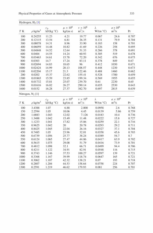
Physical Properties of Gases at Atmospheric Pressure 333
Hydrogen, H2 [1]
T K ρ kg/m3cpkJ/(kg ◦C)
μ× 106
kg/(m s)ν × 106
m2/sλ
W/(m ◦C)a×106
m2/s Pr
100 0.24255 11.23 4.21 19.77 0.067 24.6 0.707200 0.12115 13.54 6.81 26.35 0.131 79.9 0.704300 0.08078 14.31 8.96 33.90 0.183 158 0.701400 0.06059 14.48 10.82 41.69 0.226 258 0.695500 0.04848 14.52 12.64 51.33 0.266 378 0.691600 0.0404 14.55 14.24 60.93 0.305 519 0.678700 0.03463 14.61 15.78 72.20 0.342 676 0.675800 0.0303 14.7 17.24 83.11 0.378 849 0.67900 0.02694 14.83 18.65 96 0.412 1030 0.671
1000 0.02424 14.99 20.13 108.57 0.448 1230 0.6731100 0.02204 15.17 21.3 122.46 0.488 1460 0.662
200 0.0202 15.37 22.62 155.41 0.528 1700 0.6591300 0.01865 15.59 23.85 199.34 0.569 1955 0.6551400 0.01732 15.81 25.07 239.70 0.61 2230 0.651500 0.01616 16.02 26.27 290.14 0.655 2530 0.6431600 0.0152 16.28 27.37 382.70 0.697 2815 0.639
Nitrogen, N2 [1]
T K ρ kg/m3cpkJ/(kg ◦C)
μ× 106
kg/(m s)ν × 106
m2/sλ
W/(m ◦C)a × 106
m2/s Pr
100 3.4388 1.07 6.88 2.000 0.0958 2.6 0.768150 2.2594 1.05 10.06 4.45 0.0139 5.86 0.759200 1.6883 1.043 12.02 7.126 0.0183 10.4 0.736250 1.3488 1.042 15.49 11.48 0.0222 15.8 0.727300 1.1233 1.041 17.82 15.86 0.0259 22.1 0.716350 0.9625 1.042 20 20.78 0.0293 29.2 0.711400 0.8425 1.045 22.04 26.16 0.0327 37.1 0.704450 0.7485 1.05 23.96 32.01 0.0358 45.6 0.703500 0.6739 1.056 25.77 38.24 0.0389 54.7 0.7550 0.6124 1.065 27.47 44.86 0.0417 63.9 0.702600 0.5615 1.075 29.08 51.79 0.0416 73.9 0.701700 0.4812 1.098 32.1 66.71 0.0499 94.4 0.706800 0.4211 1.122 34.91 82.91 0.0548 116 0.715900 0.3743 1.146 37.53 100.27 0.0597 139 0.721
1000 0.3368 1.167 39.99 118.74 0.0647 165 0.7211100 0.3062 1.187 42.32 138.21 0.07 193 0.7181200 0.2807 1.204 44.53 158.64 0.0758 224 0.7071300 0.2591 1.219 46.62 179.93 0.081 256 0.701

334 Appendix A Tables with Physical Properties
Oxygen, O2 [1]
T K ρ kg/m3cpkJ/(kg ◦C)
μ× 106
kg/(m s)ν × 106
m2/sλ
W/(m ◦C)a × 106
m2/s Pr
100 3.945 0.962 7.64 1.936629 0.00925 2.44 0.796150 2.585 0.921 11.48 4.441006 0.0138 5.8 0.766200 1.93 0.915 14.75 7.642487 0.0183 10.4 0.737250 1.542 0.915 17.86 11.58236 0.0226 16 0.723300 1.284 0.92 20.72 16.13707 0.0268 22.7 0.711350 1.1 0.929 23.35 21.22727 0.0296 29 0.733400 0.962 0.942 25.82 26.83992 0.033 36.4 0.737450 0.8554 0.956 28.14 32.89689 0.0363 44.4 0.741500 0.7698 0.972 30.33 39.39984 0.0412 55.1 0.716550 0.6998 0.988 32.4 46.29894 0.0441 63.8 0.726600 0.6414 1.003 34.37 53.58591 0.0473 73.5 0.729700 0.5498 1.031 38.08 69.26155 0.0523 93.1 0.744800 0.481 1.054 41.52 86.32017 0.0589 116 0.743900 0.4275 1.074 44.72 104.6082 0.0649 141 0.74
1000 0.3848 1.09 47.7 123.9605 0.071 169 0.7331100 0.3498 1.103 50.55 144.5111 0.0758 196 0.7361200 0.3206 1.115 53.25 166.0948 0.0819 229 0.7251300 0.206 1.125 58.84 285.6311 0.0871 262 0.721
Carbon dioxide, CO2 [1]
T K ρ kg/m3cpkJ/(kg ◦C)
μ× 106
kg/(m s)ν × 106
m2/sλ
W/(m ◦C)A × 106
m2/s Pr
220 2.4733 0.783 11.105 4.490 0.010805 5.92 0.818250 2.1675 0.804 12.59 5.809 0.012884 7.401 0.793300 1.7973 0.871 14.958 8.322 0.016572 10.588 0.77350 1.5362 0.9 17.205 11.200 0.02047 14.808 0.755400 1.3424 0.942 19.32 14.392 0.02461 19.463 0.738450 1.1918 0.98 21.34 17.906 0.02897 24.813 0.721500 1.0732 1.013 23.26 21.67 0.03352 30.84 0.702550 0.9739 1.047 25.08 25.752 0.03821 37.5 0.695600 0.8938 1.076 26.83 30.018 0.04311 44.83 0.668
Ammonia, NH3 [2]
T K ρ kg/m3cpkJ/(kg ◦C)
μ× 106
kg/(m s)ν × 106
m2/sλ
W/(m ◦C)A × 106
m2/s Pr
220 0.3828 2.198 7.255 18.952 0.0171 20.54 0.93273 0.7929 2.177 9.353 11.796 0.022 13.08 0.9323 0.6487 2.177 11.035 17.011 0.027 19.2 0.88373 0.559 2.236 12.886 23.052 0.0327 26.19 0.87423 0.4934 2.315 14.672 29.736 0.0391 34.32 0.87473 0.4405 2.395 16.49 37.435 0.0476 44.21 0.84
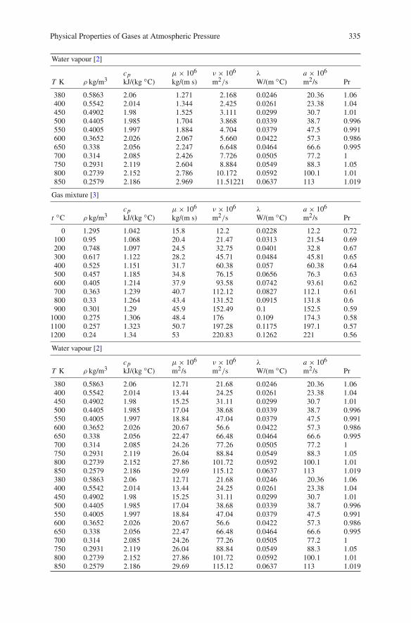
Physical Properties of Gases at Atmospheric Pressure 335
Water vapour [2]
T K ρ kg/m3cpkJ/(kg ◦C)
μ× 106
kg/(m s)ν × 106
m2/sλ
W/(m ◦C)a × 106
m2/s Pr
380 0.5863 2.06 1.271 2.168 0.0246 20.36 1.06400 0.5542 2.014 1.344 2.425 0.0261 23.38 1.04450 0.4902 1.98 1.525 3.111 0.0299 30.7 1.01500 0.4405 1.985 1.704 3.868 0.0339 38.7 0.996550 0.4005 1.997 1.884 4.704 0.0379 47.5 0.991600 0.3652 2.026 2.067 5.660 0.0422 57.3 0.986650 0.338 2.056 2.247 6.648 0.0464 66.6 0.995700 0.314 2.085 2.426 7.726 0.0505 77.2 1750 0.2931 2.119 2.604 8.884 0.0549 88.3 1.05800 0.2739 2.152 2.786 10.172 0.0592 100.1 1.01850 0.2579 2.186 2.969 11.51221 0.0637 113 1.019
Gas mixture [3]
t ◦C ρ kg/m3cpkJ/(kg ◦C)
μ× 106
kg/(m s)ν × 106
m2/sλ
W/(m ◦C)a × 106
m2/s Pr
0 1.295 1.042 15.8 12.2 0.0228 12.2 0.72100 0.95 1.068 20.4 21.47 0.0313 21.54 0.69200 0.748 1.097 24.5 32.75 0.0401 32.8 0.67300 0.617 1.122 28.2 45.71 0.0484 45.81 0.65400 0.525 1.151 31.7 60.38 0.057 60.38 0.64500 0.457 1.185 34.8 76.15 0.0656 76.3 0.63600 0.405 1.214 37.9 93.58 0.0742 93.61 0.62700 0.363 1.239 40.7 112.12 0.0827 112.1 0.61800 0.33 1.264 43.4 131.52 0.0915 131.8 0.6900 0.301 1.29 45.9 152.49 0.1 152.5 0.59
1000 0.275 1.306 48.4 176 0.109 174.3 0.581100 0.257 1.323 50.7 197.28 0.1175 197.1 0.571200 0.24 1.34 53 220.83 0.1262 221 0.56
Water vapour [2]
T K ρ kg/m3cpkJ/(kg ◦C)
μ× 106
m2/sν × 106
m2/sλ
W/(m ◦C)a × 106
m2/s Pr
380 0.5863 2.06 12.71 21.68 0.0246 20.36 1.06400 0.5542 2.014 13.44 24.25 0.0261 23.38 1.04450 0.4902 1.98 15.25 31.11 0.0299 30.7 1.01500 0.4405 1.985 17.04 38.68 0.0339 38.7 0.996550 0.4005 1.997 18.84 47.04 0.0379 47.5 0.991600 0.3652 2.026 20.67 56.6 0.0422 57.3 0.986650 0.338 2.056 22.47 66.48 0.0464 66.6 0.995700 0.314 2.085 24.26 77.26 0.0505 77.2 1750 0.2931 2.119 26.04 88.84 0.0549 88.3 1.05800 0.2739 2.152 27.86 101.72 0.0592 100.1 1.01850 0.2579 2.186 29.69 115.12 0.0637 113 1.019380 0.5863 2.06 12.71 21.68 0.0246 20.36 1.06400 0.5542 2.014 13.44 24.25 0.0261 23.38 1.04450 0.4902 1.98 15.25 31.11 0.0299 30.7 1.01500 0.4405 1.985 17.04 38.68 0.0339 38.7 0.996550 0.4005 1.997 18.84 47.04 0.0379 47.5 0.991600 0.3652 2.026 20.67 56.6 0.0422 57.3 0.986650 0.338 2.056 22.47 66.48 0.0464 66.6 0.995700 0.314 2.085 24.26 77.26 0.0505 77.2 1750 0.2931 2.119 26.04 88.84 0.0549 88.3 1.05800 0.2739 2.152 27.86 101.72 0.0592 100.1 1.01850 0.2579 2.186 29.69 115.12 0.0637 113 1.019

336 Appendix A Tables with Physical Properties
Physical Properties of Some Saturated Liquid
Ammonia, NH3 [4]
t ◦C ρ kg/m3cpkJ/(kg ◦C)
μ× 106
kg/(m s)ν × 106
m2/sλ
W/(m ◦C)a × 107
m2/s Pr
–50 703.69 4.463 306.11 0.435 0.547 1.742 2.6–40 691.68 4.467 280.82 0.406 0.547 1.775 2.28–30 679.34 4.467 262.9 0.387 0.549 1.801 2.15–20 666.69 4.509 254.01 0.381 0.547 1.819 2.09–10 653.55 4.564 247.04 0.378 0.543 1.825 2.07
0 640.1 4.635 238.76 0.373 0.54 1.819 2.0510 626.16 4.714 230.43 0.368 0.531 1.801 2.0420 611.75 4.798 219.62 0.359 0.521 1.775 2.0230 596.37 4.89 208.13 0.349 0.507 1.742 2.0140 580.99 4.999 197.54 0.34 0.493 1.701 250 564.33 5.116 186.23 0.33 0.476 1.654 1.99
Carbon dioxide, CO2 [4]
t ◦C ρ kg/m3cpkJ/(kg ◦C)
μ× 106
kg/(m s)ν × 106
m2/sλ
W/(m ◦C)a × 107
m2/s Pr
–50 1156.34 1.84 137.61 0.119 0.085 0.4021 2.96–40 1117.77 1.88 131.9 0.118 0.1011 0.481 2.45–30 1076.76 1.97 125.98 0.117 0.1116 0.5272 2.22–20 1032.39 2.05 118.72 0.115 0.1151 0.5445 2.12–10 983.38 2.18 111.12 0.113 0.1099 0.5133 2.2
0 926.99 2.47 100.11 0.108 0.1045 0.4578 2.3810 860.03 3.14 86.86 0.101 0.0971 0.3608 2.820 772.57 5 70.3 0.091 0.0872 0.2219 4.130 597.81 36.4 47.82 0.08 0.0703 0.0279 28.7
Sulphur dioxide, SO2 [4]
t ◦C ρ kg/m3cpkJ/(kg ◦C)
μ× 106
kg/(m s)ν × 106
m2/sλ
W/(m ◦C)a × 107
m2/s Pr
–50 1560.84 1.3595 755.45 0.484 0.242 1.141 4.24–40 1536.81 1.3607 651.61 0.424 0.235 1.130 3.74–30 1520.64 1.3616 564.16 0.371 0.230 1.117 3.31–20 1488.60 1.3624 482.31 0.324 0.225 1.107 2.93–10 1463.61 1.3628 421.52 0.288 0.218 1.097 2.62
0 1438.46 1.3636 369.68 0.257 0.211 1.081 2.3810 1412.51 1.3645 327.7 0.232 0.204 1.066 2.1820 1386.40 1.3653 291.14 0.210 0.199 1.050 2.0030 1359.33 1.3662 258.27 0.190 0.192 1.035 1.8340 1329.22 1.3674 229.96 0.173 0.185 1.019 1.7050 1299.10 1.3683 210.45 0.162 0.177 0.999 1.61
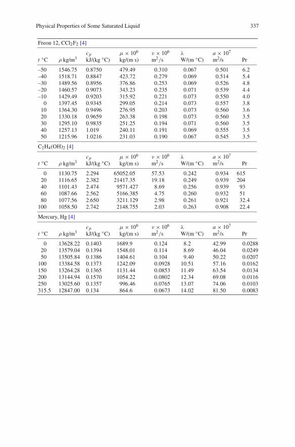
Physical Properties of Some Saturated Liquid 337
Freon 12, CCl2F2 [4]
t ◦C ρ kg/m3cpkJ/(kg ◦C)
μ× 106
kg/(m s)ν × 106
m2/sλ
W/(m ◦C)a × 107
m2/s Pr
–50 1546.75 0.8750 479.49 0.310 0.067 0.501 6.2–40 1518.71 0.8847 423.72 0.279 0.069 0.514 5.4–30 1489.56 0.8956 376.86 0.253 0.069 0.526 4.8–20 1460.57 0.9073 343.23 0.235 0.071 0.539 4.4–10 1429.49 0.9203 315.92 0.221 0.073 0.550 4.0
0 1397.45 0.9345 299.05 0.214 0.073 0.557 3.810 1364.30 0.9496 276.95 0.203 0.073 0.560 3.620 1330.18 0.9659 263.38 0.198 0.073 0.560 3.530 1295.10 0.9835 251.25 0.194 0.071 0.560 3.540 1257.13 1.019 240.11 0.191 0.069 0.555 3.550 1215.96 1.0216 231.03 0.190 0.067 0.545 3.5
C2H4(OH)2 [4]
t ◦C ρ kg/m3cpkJ/(kg ◦C)
μ× 106
kg/(m s)ν × 106
m2/sλ
W/(m ◦C)a × 107
m2/s Pr
0 1130.75 2.294 65052.05 57.53 0.242 0.934 61520 1116.65 2.382 21417.35 19.18 0.249 0.939 20440 1101.43 2.474 9571.427 8.69 0.256 0.939 9360 1087.66 2.562 5166.385 4.75 0.260 0.932 5180 1077.56 2.650 3211.129 2.98 0.261 0.921 32.4
100 1058.50 2.742 2148.755 2.03 0.263 0.908 22.4
Mercury, Hg [4]
t ◦C ρ kg/m3cpkJ/(kg ◦C)
μ× 106
kg/(m s)ν × 106
m2/sλ
W/(m ◦C)a × 107
m2/s Pr
0 13628.22 0.1403 1689.9 0.124 8.2 42.99 0.028820 13579.04 0.1394 1548.01 0.114 8.69 46.04 0.024950 13505.84 0.1386 1404.61 0.104 9.40 50.22 0.0207
100 13384.58 0.1373 1242.09 0.0928 10.51 57.16 0.0162150 13264.28 0.1365 1131.44 0.0853 11.49 63.54 0.0134200 13144.94 0.1570 1054.22 0.0802 12.34 69.08 0.0116250 13025.60 0.1357 996.46 0.0765 13.07 74.06 0.0103315.5 12847.00 0.134 864.6 0.0673 14.02 81.50 0.0083

338 Appendix A Tables with Physical Properties
Water, H2O [2]
t ◦C ρ kg/m3cpkJ/(kg ◦C)
μ× 106
kg/(m s)ν × 106
m2/sλ
W/(m ◦C)a × 106
m2/s Pr
0 999.9 4.217 1752.5 1.7527 0.569 0.13494 12.9910 999.7 4.193 1299.2 1.2996 0.586 0.13980 9.3020 998.2 4.182 1001.5 1.0033 0.602 0.1442 6.9630 995.7 4.179 797 0.8004 0.617 0.14828 5.440 992.2 4.179 651.3 0.6564 0.630 0.14953 4.3250 988.1 4.181 544 0.5450 0.643 0.15408 3.5460 983.2 4.185 460 0.4679 0.653 0.15870 2.9770 977.8 4.190 400.5 0.4014 0.662 0.15834 2.5480 971.8 4.197 351 0.3612 0.669 0.16403 2.2090 965.3 4.205 311.3 0.3225 0.675 0.16629 1.94
100 958.4 4.216 279 0.2911 0.680 0.16829 1.73110 951.0 4.229 252.2 0.2652 0.683 0.16983 1.56120 943.1 4.245 230 0.2439 0.685 0.17110 1.43130 934.8 4.263 211 0.2257 0.687 0.17239 1.31140 926.1 4.285 195 0.2106 0.687 0.17312 1.22150 917.0 4.310 181 0.1974 0.686 0.17357 1.14160 907.4 4.339 169 0.1862 0.684 0.17373 1.07170 897.3 4.371 158.5 0.1766 0.681 0.17363 1.02180 886.9 4.408 149.3 0.1683 0.676 0.17291 0.97190 876.0 4.449 141.2 0.1612 0.671 0.17217 0.94200 863.0 4.497 133.8 0.1550 0.664 0.17109 0.91210 852.3 4.551 127.3 0.1494 0.657 0.16938 0.88220 840.3 4.614 121.5 0.1446 0.648 0.16713 0.86230 827.3 4.686 119.7 0.145 0.639 0.16483 1.185240 813.6 4.770 111.4 0.1369 0.629 0.16208 0.85250 799.0 4.869 107 0.1339 0.617 0.15860 0.84260 784.0 4.985 103 0.1314 0.604 0.15455 0.85270 767.9 5.13 99.4 0.1294 0.589 0.14952 0.86280 750.7 5.3 96.1 0.1280 0.573 0.14402 0.89290 732.3 5.51 93 0.1270 0.558 0.14300 0.92300 712.5 5.77 90.1 0.1265 0.540 0.13136 0.96
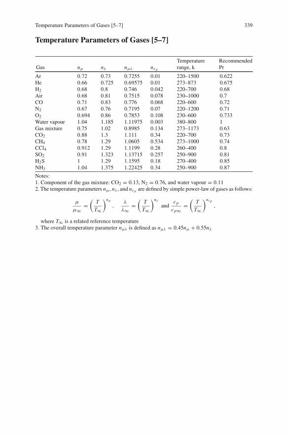
Temperature Parameters of Gases [5–7] 339
Temperature Parameters of Gases [5–7]
Gas nμ nλ nμλ ncp
Temperaturerange, k
RecommendedPr
Ar 0.72 0.73 0.7255 0.01 220–1500 0.622He 0.66 0.725 0.69575 0.01 273–873 0.675H2 0.68 0.8 0.746 0.042 220–700 0.68Air 0.68 0.81 0.7515 0.078 230–1000 0.7CO 0.71 0.83 0.776 0.068 220–600 0.72N2 0.67 0.76 0.7195 0.07 220–1200 0.71O2 0.694 0.86 0.7853 0.108 230–600 0.733Water vapour 1.04 1.185 1.11975 0.003 380–800 1Gas mixture 0.75 1.02 0.8985 0.134 273–1173 0.63CO2 0.88 1.3 1.111 0.34 220–700 0.73CH4 0.78 1.29 1.0605 0.534 273–1000 0.74CCl4 0.912 1.29 1.1199 0.28 260–400 0.8SO2 0.91 1.323 1.13715 0.257 250–900 0.81H2S 1 1.29 1.1595 0.18 270–400 0.85NH3 1.04 1.375 1.22425 0.34 250–900 0.87
Notes:1. Component of the gas mixture: CO2 = 0.13, N2 = 0.76, and water vapour = 0.112. The temperature parameters nμ, nλ, and ncp are defined by simple power-law of gases as follows:
μ
μ∞=(
T
T∞
)nμ
,λ
λ∞=(
T
T∞
)nλ
andcp
cp∞=(
T
T∞
)ncp
,
where T∞ is a related reference temperature3. The overall temperature parameter nμλ is defined as nμλ = 0.45nμ + 0.55nλ
340 Appendix A Tables with Physical Properties
References
1. F.P. Incropera, D.P. Dewitt, Fundamen300tals of Heat Transfer (Wiley, New York, NY, 1981)2. T. Cebeci, P. Brabshaw, Physical and Computational Aspects of Convective Heat Transfer
(Springer, New York, NY, 1984)3. Shiming Yang, Heat Transfer, 2nd Ed., (Higher Education, Beijing, 1987)4. E.R.G. Eckert, R.M. Drake, Heat and Mass Transfer, 2nd edn. (McGraw-Hill Book, New York,
NY, 1959)5. D.Y. Shang, B.X. Wang, Effect of variable thermophysical properties on laminar free convection
of gas. Int. J. Heat Mass Transf. 33(7), 1387–1395 (1990)6. D.Y. Shang, B.X. Wang, Effect of variable thermophysical properties on laminar free convection
of polyatomic gas. Int. J. Heat Mass Transf. 34(3), 749–755 (1991)7. D.Y. Shang, Free Convection Film Flows and Heat Transfer (Springer, Berlin, Heidelberg and
New York, NY, 2006)

Index
AAbsolute viscosity, 37, 72, 121, 128, 150, 176,
243of gas, 277of vapour, 277of vapour–gas mixture, 243, 277
Adiabatic Eckert number, 10–11, 56, 79, 81,84, 93, 98, 101, 109, 112, 143
Average heat transfer coefficient, 83, 102, 137,159, 211, 293
Average heat transfer rate, 83, 102, 136, 158Average kinetic viscosity, 121Average Nusselt number, 84, 86, 102, 105–106,
137, 140, 159, 211, 213, 293Average Prandtl number, 10–11, 56, 79, 81, 84,
93, 98, 101, 109, 112, 143Average skin-friction coefficient, 88, 90–92,
110, 145–146, 156, 166, 170, 172
BBasic dimensions, 53–54Boundary temperature ratio, 119, 129,
131–134, 137–138, 140–142,149, 167
Buckingham π-theorem, 51, 53Bulk vapour mass fraction, 10, 13, 274, 282,
284–285, 288, 291, 294, 296–298,304, 321–322
CCalculation procedure, 201–202, 273, 280–281Complete similarity mathematical model
of forced convection, 1, 12, 75,175–194, 198, 205, 210, 241–271,274, 292
Concentration boundary layer, 1–2, 7, 242Condensate liquid film thickness, 12, 14,
201, 217, 230, 238, 273, 280, 285,287–288
Condensate mass–energy transformation coefficient, 227,
236, 310–314, 327–energy transformation equation, 1, 12,
209, 225–230, 236, 239, 291, 310,312–313, 321–322, 327
flow rate, 12, 210, 217–218, 222, 224,226–227, 230, 236–237, 239, 292,304–305, 310, 312–313, 320–323,326–327
parameter, 12, 210, 217–218, 222,224, 226–227, 230, 236, 239, 292,304–305, 310, 312–313, 321–322
Condensation heat transfer, 225–226Condensation mass transfer, 3–7, 12–14, 68,
75, 176–177, 209–239, 241–242,274, 282, 291–327
Consideration of variable physical properties,6, 8–9, 30–37, 43, 47–48, 52,69–70, 75–76, 98–100, 119–146,150, 156–159, 161, 167, 169–172,177, 179–180, 194, 210, 274, 292
Consideration of viscous thermal dissipation,10–11, 37, 83, 86, 89, 91, 93–117
Control volume, 21–23, 26
DDensity factor
of gas, 277of vapour, 277of vapour–gas mixture, 277
Density of gas, 128, 275–277Density of vapour, 275, 277Density of vapour–gas mixture, 275–276Dimensionless similarity parameters
(Number), 53–56Dimensionless similarity variables for film
condensation, 179, 245
D.Y. Shang, Theory of Heat Transfer with Forced Convection Film Flows,Heat and Mass Transfer, DOI 10.1007/978-3-642-12581-2,C© Springer-Verlag Berlin Heidelberg 2011
341

342 Index
Dimensionless similarity variables for forcedconvection, 95, 121, 151
Dimensionless temperature, 9–14, 47, 62,67, 69, 77, 79, 84, 89–92, 93, 95,98, 101, 103, 105, 111–112, 114,116, 122, 128–129, 131, 136, 138,140–142, 149–151, 154, 156, 158,161, 163, 166–168, 176, 179–180,198–199, 202, 205–206, 210–213,230, 235–236, 238, 245–246, 274,287, 292, 294–297, 312, 316–317,319, 321–322
Dimensionless velocity components, 2, 52, 58,62, 67–69, 77–79, 89, 95, 98, 122,128, 131, 141, 151, 179–180, 215,230, 246, 302, 316–317
Dimensionless wall temperature gradient,12–13, 84–86, 101, 103–105, 137,159–164, 313, 321
EEckert number, 2, 10–11, 83, 93–94, 97–98,
103, 107–109, 111–113, 115–117,120, 137, 142–143, 146, 159,168–169, 172
Effect of variable physical properties, 4–6,9–11, 120, 156–157, 159, 161, 164,167, 170–171
Effect of viscous thermal dissipation, 10–11,94, 143, 169
Enthalpy, 29, 94
FFalkner-Skan type transformation, 1–2, 4, 7–8,
13, 39–49Film condensation of vapour–gas mixture,
1–3, 5–7, 9–10, 12–14, 241–271,273–289, 291–327
Film condensation of vapours, 1–14, 177–180,193–194, 197–198, 226, 230–231,241–271, 273–288, 291–327
Forced convection, 1–11, 14, 30–37, 39–49,51–70, 75–117, 119–146, 149–172,175–177, 179–180, 197, 209–210,320–321
GGas mass fraction, 288Group theory, 41, 46, 68
HHeat and mass transfer of forced film
condensation, 1–5, 7, 12, 62, 176,198, 209–239, 241–242, 282, 288,291–327
Heat transfer coefficient, 53, 83, 101–102,119, 136–137, 142, 158–159, 168,210–211, 292–293
Heat transfer of laminar forced convection, 1,6, 10–11, 34, 86, 93–117, 120, 150
IIncrement momentum, 23, 131Interfacial boundary conditions, 193Interfacial dimensionless velocity components,
217–218, 222, 224Interfacial vapour mass fraction, 7, 13, 246,
281–282, 292, 297–299Interfacial vapour saturated temperature, 1,
3, 5, 7, 10, 13–14, 242, 245–246,271, 281–282, 294, 297–301, 304,310–313, 321–323, 325, 327
Intermediate similarity variable function,52, 70
Internal energy, 27–28
LLaminar forced boundary layer, 7, 31, 61Laminar forced film condensation of vapour,
1–13, 177–180, 193–194, 197–198,226, 230–231, 241–271, 273–288,291–327
Laminar forced film condensation ofvapour–gas mixture, 1–3, 5–7,9–10, 12–14, 241–271, 273–289,291–327
Latent heat, 12, 205–206, 225–227, 282, 311Local condensate mass flow rate, 210,
217–218, 222, 224, 226–227, 230,236–237, 239, 292, 304–305, 310,312–313, 320–323, 326–327
Local density of gas, 275Local density of vapour, 275Local heat transfer coefficient, 83, 101, 136,
158, 210, 292Local heat transfer rate, 82, 101, 136, 158,
210, 292Local Nusselt number, 55, 83, 102, 136, 158,
211, 293Local Reynolds number with constant physical
properties, 95, 324Local Reynolds number with variable physical
properties, 121, 151, 179, 245Local Schmidt number, 268Local skin-friction coefficient with constant
physical properties, 79Local skin-friction coefficient with variable
physical properties, 133

Index 343
MMass force, 23, 27
NNew similarity analysis method, 2–3, 8–12,
14, 39, 51–70, 75, 77–80, 89, 112,121, 141, 146, 149, 151, 167, 176,193–194, 198, 230, 242, 270–271
Non-condensable gas, 16, 241, 244, 294, 322
OOverall temperature parameter, 131, 138, 140
PPhysical property factors, 9, 11, 13, 128–129,
149, 152–154, 165, 167, 193,197–200, 230–231, 234, 274–275,279–280, 287, 313, 318–319
QQuantitative grade analysis, 30–31
RReference vapour saturation temperature, 294,
322Reference wall subcooled grade, 294, 296–298,
304–305, 313, 322–323Reference wall subcooled temperature, 294,
298
SSaturation temperature, 1, 3, 5, 7, 10, 13–14,
242, 245–246, 281–282, 292, 294,297–301, 304, 310–313, 321–323,325, 327
Schmidt number, 268Shear force, 4–7, 11–12, 23, 28, 177, 179, 193,
197, 242, 244, 270, 274, 287Similarity variables, 2, 11, 40–44, 47–48,
52, 56–63, 67–70, 77, 86–87,89, 95–96, 110, 122, 164–165,179–180, 194, 230–232, 245–247,270–271, 313, 316–317
Simple power-law equations, 340Skin-friction coefficient, 79–82, 88, 90–92,
110, 133–135, 141, 145–146,156–157, 166, 170, 172
Species conservation equation, 244Specific enthalpy, 29Stream function, 7, 41, 45–46, 48, 51–52, 68Surface force, 23, 27–28
TTemperature parameter, 9, 11, 129–131,
133–134, 138, 140–142, 149, 197,278, 340
Thermal conductivity factorof gas, 278of vapour, 278of vapour–gas mixture, 278
Thermal conductivity of gas, 141, 278–279Thermal conductivity parameter, 129, 137,
146, 279, 282Thermal conductivity of vapour, 278–279, 282,
310Thermal conductivity of vapour–gas mixture,
278Total condensate mass flow rate, 216, 302Total heat transfer rate, 83, 86, 102, 136, 158,
211, 239, 293Treatment of variable physical properties,
8–9, 11, 128–131, 152, 197–198,274–280
VVapour–gas mixture, 1–3, 5–10, 12–13,
242–247, 260, 263, 270–271,273–289, 291–327
Vapour mass diffusion coefficient, 282Vapour mass fraction, 7, 10, 13, 244, 246–247,
273–274, 281–282, 284–285,287–288, 292, 294, 296–299, 304,321–322
Vapour superheated grade, 10, 12, 202,205–206, 209, 212, 218, 226, 230,236
Vapour superheated temperature, 194Variable physical properties, 2, 4–6, 8–11,
13, 30–37, 39, 47–48, 52, 68–70,75–92, 94–95, 98–106, 108, 110,112–117, 119–146, 149–172,176–177, 179–180, 193–194,197–198, 200, 205–206, 210, 270,274–275, 291–292
Viscosity factorof gas, 279of vapour, 278–279of vapour–gas mixture, 278
Viscosity parameter, 129, 137, 279, 282Viscous thermal dissipation, 2, 10–11, 28,
33–35, 37, 39, 47, 52, 75–92,

344 Index
93–117, 120–121, 136–137,142–144, 146, 159, 168–170, 172
WWall dimensionless temperature gradient,
10–12, 14, 84, 98, 101, 111–112,114, 116, 136, 138, 140–142,150, 156, 158, 161, 163, 166–168,202, 205–206, 210, 212–213, 230,235–236, 238–239, 292, 294–297,312, 321–322
Wall dimensionless velocity gradient,134–135, 157
Wall skin shear force, 80, 133
Wall subcooled grade, 10, 12, 202, 205–206,212, 217–218, 230, 236, 273,294, 296–298, 300, 304–305, 313,322–323
Wall subcooled temperature, 7, 227, 282,286–288, 293–295, 298–299, 301,306–309, 325


![J org Pretz arXiv:2005.12203v1 [physics.class-ph] 25 May 2020 › pdf › 2005.12203.pdf · (t)/ m mass 1 mass 2 mass 3 mass 4 mass 5 mass 6 mass 7 mass 8 mass 9 mass 10 Figure 2.](https://static.fdocuments.us/doc/165x107/5f1ec529f26656179f60ee75/j-org-pretz-arxiv200512203v1-25-may-2020-a-pdf-a-200512203pdf-t.jpg)
![لﻮﺻا ﻲﺑﺎﻳرازﺎﺑsv.20file.org/up1/1437_0.pdfZZZ 3UR]KHKD LU ﻪﺑ ﻢﻳﺪﻘﺗ ،مﺮﺘﺧد و مﺮﺴﻤﻫ ﻦﻴﻤﺳﺎﻳ و ﻢﻳﺮﻣ ZZZ 3UR]KHKD](https://static.fdocuments.us/doc/165x107/5f744978100e183e04671820/ii-iiiiiisv-zzz-3urkhkd-lu-ii-iiiii-oeiii.jpg)