Health Status and Labour Force Status of Older Working-Age...

227AUTHORS

Title

227AUSTRALIAN JOURNAL OF LABOUR ECONOMICS

Vol. 10, No. 4, December 2007, pp 227 - 252

Health Status and Labour Force Statusof Older Working-Age Australian Men

Lixin Cai and Guyonne Kalb, The University of Melbourne

AbstractThis research uses the Household, Income and Labour Dynamics in Australia (HILDA)Survey to investigate the impacts of health on labour force status of older working-age Australian men. We estimate a model that exploits the longitudinal nature of thedata and takes the correlation between the two error terms in the health and labourforce status equations into account. The results show that controlling for unobservedheterogeneity and the correlation between the two equations is important. It is alsofound that any restriction on the correlation between the two equations appears tolead to underestimation of the direct health effects.

1. IntroductionConcerns regarding early retirement by older working-age men combined with anageing population have led many industrialised nations to develop policies encouragingolder male workers to remain in the labour force. Due to its direct impact on productivityand indirect effect on the preference between income and leisure, health plays animportant role in individuals’ labour supply decisions (Currie and Madrian, 1999). Agood understanding of how health influences labour force participation among olderworkers would facilitate the development of effective policies, aimed at keeping olderworkers in the labour market, and result in a better estimate of the costs of healthlimitations to the economy (Chirikos, 1993).

The effect of health on labour market activity of older male workers has beenunder extensive examination in the US and other industrialized countries, with thegeneral finding that health has a significant effect on labour force participation (e.g.

Address for correspondence: Lixin Cai, Melbourne Institute of Applied Economic and SocialResearch, The University of Melbourne, Victoria 3010. Email: [email protected]: We would like to thank Jeff Borland, John Creedy, Jan van Ours, Mark Woodenand workshop participants at the University of Melbourne and at Tilburg University for valuablecomments and suggestions. This paper is based on research being conducted as part of the researchprogram ‘The Dynamics of Economic and Social Change: An Analysis of the Household, Incomeand Labour Dynamics in Australia Survey’. It is supported by an Australian Research CouncilDiscovery Grant (DP0342970). The paper uses the data in the confidentialised unit record filefrom the Department of Families, Housing, Community Services and Indigenous Affairs’(FaHCSIA) Household, Income and Labour Dynamics in Australia (HILDA) Survey, which ismanaged by the Melbourne Institute of Applied Economic and Social Research. The findings andviews reported in the paper, however, are those of the authors and should not be attributed to eitherFaHCSIA or the Melbourne Institute.© The Centre for Labour Market Research, 2007

228AUSTRALIAN JOURNAL OF LABOUR ECONOMICSDECEMBER 2007

Disney et al., 2006; Au et al., 2005; Campolieti, 2002; Dwyer and Mitchell, 1999;Stern, 1989; Sickles and Taubman, 1986). Most previous studies rely on cross-sectionaldata, with the exception of Disney et al. (2006), Au et al. (2005) and Sickles andTaubman (1986). The current study contributes to the literature by using the longitudinalnature of panel data, which allows better control for unobserved heterogeneity,decomposing it into a time-variant and a time-invariant component. Therefore, moreefficient estimates for the health effects on labour force status can be provided usingthese data than a cross-sectional analysis could.

Since it is highly likely that similar unobserved factors affect both health andlabour force status, we estimate a model that takes into account the correlation betweenthe two error terms in the health and labour force participation equations. This controlsfor the potential endogeneity of the health variable arising from unobservedheterogeneity. The results show that controlling for the unobserved heterogeneity andthe correlation between the two equations is important. That is, the estimated variancesof the unobserved heterogeneity terms are significantly different from zero in bothequations and the two error terms are found to be correlated. It is also found thattreating health as an exogenous variable leads to underestimation of its direct effecton labour force participation.

The current study also serves to provide further empirical evidence on theeffect of health on labour force status in Australia. Despite a large body of overseasliterature, there are relatively few Australian studies on this issue. Cai and Kalb (2006)used the first wave of the Household, Income and Labour Dynamics in Australia(HILDA) Survey, finding that health has a significant effect on labour force participationfor younger and older men and women, with the reverse effect of labour force statuson health only evident for younger men. Using the 1998 Survey of Disability, Ageingand Carers (SDAC), Wilkins (2004) found that the presence of a disability decreasesthe probability of participation in the labour force by 0.24 for males and 0.20 forfemales. The disability status in SDAC is derived from a combination of long-termhealth conditions and specific activity restrictions, and thus is a relatively narrowmeasure of health. Based on the Australian National Health Survey Data, Zhang et al.(2006) found that among three chronic types of diseases (heart disease, diabetes, andmental health), mental health has the largest effect on labour force participation,followed by diabetes.

The paper is organised as follows. Section 2 provides some theoreticalbackground on the relationship between health and labour supply. The econometricmodel and estimation strategy are described in section 3. Section 4 discusses the dataand variables, followed by the estimation results in section 5. Finally, section 6concludes.

2. Conceptual FrameworkThere are several reasons why health may be an important factor in an individual’sdecision on labour supply. First, health is a determinant of productivity because anindividual’s capacity to fulfil a job’s requirements is closely related to the person’shealth. Health is therefore often regarded as a form of human capital that is valued byboth employers and employees (Currie and Madrian, 1999). As such, individuals with

229LIXIN CAI AND GUYONNE KALB

Health Status and Labour Force Status of Older Working-Age Australian Men

better health can command higher wages, which, other things equal, increases a person’slabour force participation probability. Second, health may influence individuals’ laboursupply through shifting preferences between income and leisure. For example, poorhealth may lead individuals to value leisure time more, perhaps because the time neededto care for one’s health increases with ill health or because the burden of work mayincrease with poor health. On the other hand, poor health may cause people to requiremore income due to costs associated with poor health. Third, because life expectancyis determined by health, changes in health may change the time horizon over whichlabour supply decisions are made. For example, poor health may make early withdrawalfrom the labour market more attractive (Chirikos, 1993).

Although health is predetermined partly as an endowment at birth, health isnot exogenous over one’s lifetime. Like other forms of human capital, people canmake investments into health to make improvements or reduce the depreciation of thestock of health.1 Because this investment requires resources, such as time for recreationor exercise and income for health care, health is endogenous in the sense that peoplehave to make choices in the production of health. As such, people’s health may also beaffected by labour supply, especially a person’s labour supply history, because pastlabour supply may determine the availability of resources that can be utilised to investinto health. There are also arguments that people’s current health may be affected bycurrent labour market activities. For example, boredom or general lack of activity innon-participation may lead to a deterioration of health (Stern, 1989; Sickles andTaubman, 1986). However, given the way in which the health stock evolves, it isunlikely that current labour market activity plays a significant role in current healthstatus, although it may affect future health directly and indirectly.

The relationship between health and labour supply can be formalised in aneconomic model that is based on the assumption that individuals maximise anintertemporal utility function (Currie and Madrian, 1999). In such a model, healthtogether with labour supply and consumption of other goods enter the utility functionas endogenous choice variables. In principle, it is possible to derive demand functionsfor health, for leisure and for other consumption goods from this economic model. Inparticular, the model can be solved to yield a conditional labour supply function inwhich labour supply depends on the endogenous health variable and a set of otherexogenous variables. In this paper, we do not formally derive this model but simplyspecify the variables entering the labour force equation following the literature onlabour supply.

3. Statistical Model and Estimation StrategyBased on the framework described in section 2, an econometric model is derived forestimation. We adopt a recursive model of health and labour force status where currenthealth affects current labour force status but where there are no feedback effects fromcurrent labour force status to current health. As an empirical test to confirm the validityof our recursive model, we estimated a simultaneous equation model. Using a two-

1 Unlike education, however, health as a form of human capital is subject to adverse shocks, suchas the occurrence of illness or an accident, which may reduce health stock dramatically. Healthinvestments can be used to improve health or to prevent adverse health shocks.


stage maximum likelihood estimation method, which provides consistent estimates,we found that current labour force status has no significant effect on current health.This result provides empirical support for the recursive model. The recursive modelstill accounts for the endogeneity of health arising from correlated unobservabledeterminants of health and labour supply.

Model SpecificationThe focus of this paper (as well as that of related literature) is on the labour forcestatus equation. The health equation mainly serves to control for the endogeneity ofhealth resulting from unobserved heterogeneity. The system of equations is as follows:

l*it = f (h

it) + x

L,it β

L + ε

L,it , (1)

h*it = x

h,it β

h + ε

h,it (i = 1,..., N; t = 1,..., T ). (2)

Equation (1) is for labour force status and equation (2) for health status; l*it

andh*

it are the latent dependent variables, representing the value of being in the labour

force and health stock; xh,it

, and xL,it

are the two sets of exogenous or predeterminedvariables; β

h and β

L are the structural coefficients corresponding to x

h,it, and x

L,it

respectively; f (hit) is a function representing the effect of observed health on labour

force status; and εh,it

and εL,it

, are the structural disturbances.The unobserved dependent variables l*

it and h*

it, underlying the model, need to

be linked to their observed discrete counterparts lit and h

it. In our data, five ordered

health levels are available. Although unemployment can be identified from the data,we only distinguish two labour force states in the paper, participation and non-participation, with labour force participation including unemployment, because theproportion of unemployed is very small (only about 3 percent) in the sample.2 Thecorresponding observed values of the dependent variables are:

(3)

(4)

2 An alternative division of labour force status is employed versus not employed. We preferparticipation versus non-participation because an individual’s participation is a personal choice(or a labour supply decision), while a person’s employment also depends on labour demand. Byusing participation versus non-participation, we focus on individuals’ labour supply decisions.However, we found that the results using the alternative division are very similar to the results inthis paper.



Equations (1), (2), (3) and (4) constitute a system of equations. In addition,for the effect of health we specify

f (h) = α1 × excellent + α

2 × very _ good + α

3 × good +α

4 × fair. (5)

The longitudinal nature of the data set is exploited by using a conventionalerror components specification for the two disturbances.3 Specifically, we decomposeeach of the two disturbances into two parts, a time-invariant component, µ

j,i , and a

time-variant component, νj,it

:

εj,it

= µj,i + ν

j,it (j = h, L). (6)

The time-invariant error component allows for improved control for unobservedheterogeneity compared to cross-sectional analysis. Although µ

j,i ,can be estimated

either as a fixed or as a random effect in a general framework of panel data models, thediscrete nature of the observed dependent variables in our data requires the assumptionof a random effect for the time-invariant component (Hsiao, 2003).4 The time-invariantcomponent introduces a correlation among the disturbances in different time periodsof the same equation:

(7)

where δj(µ)

is the variance of the time-invariant component and δj(ν)

is the variance ofthe time-variant component.

The correlation across the two equations may occur through different scenarios,each leading to a different variance-covariance structure for the disturbance terms.First, if the correlation only comes from the time-invariant component, that is, cov(ν

h,is,

νL,it

) = δhL(ν)

= 0 for all s and t, and cov(µh,i

, µ

L,i ) = δ

hL(µ) ≠ 0, the two equations are

correlated in the same time period and across different time periods,

cov(εh,is

, ε

L,it ) = δ

hL(µ) , for all s and t. (8)

A second scenario is for the correlation to come from the same period time-

variant component only, that is, , and cov(µh,i

, µ

L,i ) = 0.

3 We do not estimate a dynamic model in which labour force participation and health in previousperiods are allowed to affect current labour force participation and health, since three years of datawould not be sufficient to estimate this type of model.4 By assuming a random effect, we rule out the possibility that the individual effects (that is, thetime-invariant error components) are correlated with the right-hand side explanatory variablesexcept for health in the labour force equation. The health variable in the labour force equation iscorrelated with the individual effects in that equation through the correlation of the individualeffects in the error terms in the two equations.


In this case, the two equations are only correlated in the same time period andnot correlated across time periods,

(9)

In the third alternative, the correlation arises from both components, that is

cov(µh,i

, µ

L,i ) δ

hL(µ) ≠ 0, and implying

(10)

Combining (7) with one of (8), (9) or (10) defines the variance-covariancematrix of the disturbance terms5. We further assume that the two components of eachdisturbance are independently normally distributed, which means that the twodisturbances are jointly normally distributed. For identification purposes, δ

j(ν) with

j = h, L needs to be normalised to one in the model. Consequently, the covariance δhL(ν)

is equal to the correlation coefficient between the two time-variant error components.The statistical model is similar to that used in Sickles and Taubman (1986),

although they estimated the model based on the assumption that the correlation acrossthe two equations is solely due to the same period time-variant component. That is,the variance-covariance of the disturbance terms is defined by (7) and (9). Thespecification in (9) is based on the assumption that both health and labour force statusare affected by shocks occurring in the same period and the impact of the shocks donot last for more than one period. The assumption implied in specification (8) is thatthere may be some permanent unobservable personal attributes or preferences thataffect both health and labour force status. The specification in (10) takes bothpossibilities into account, leaving all options open, and thus is more general. In themain specification of the model, we use the variance-covariance structure resultingfrom (7) and (10), extending Sickles and Taubman (1986).

The parameters to be estimated are the coefficientsβh and β

L in equations (1)

and (2), α1 to α

4 in equation (5); the cut-off points A

0 to A

3in equations (3) (B

0 is

normalised to zero after including a constant term in the labour force participationequation); and the parameters in the variance-covariance matrix of the disturbance terms.

Estimation ProcedureIn principle, the parameters can be estimated using the maximum likelihood estimator(MLE) by assuming a joint density f (ε

hi,1 ,..., ε

h,iT ; ε

li,1 ,..., ε

l,iT ). However, a computational

issue arises when T≥2 and evaluation of at least a four-dimensional integral is required.5 In principle, it is possible to allow the time-variant component to be correlated across differenttime periods of the same equation. For example, it could follow a first order autoregressive process.However, because only three waves of data were available at the time of analysis, not much gainwas expected from this specification. It will be left for future research when more waves becomeavailable.



In our case, with three waves of data, evaluation of six-dimensional integrals for observingeach specific configuration of health-labour force state for the same individual over thethree time periods would be required if traditional MLE were to be used. This renderssuch estimation infeasible. However, recently developed simulation-based estimationtechniques provide a feasible approach to overcome this problem (Stern, 1997).

Simulation-based estimation procedures replace functions (usually integrals),which are computationally intractable when using numerical or analytical methods,with random approximations for these functions. There are generally two approachesto simulation-based estimators: direct simulation of the likelihood function or indirectlikelihood simulation by using an expression for the score of the likelihood (Hyslop,1999). In this paper the former approach, known as maximum simulated likelihood(MSL).6 Following Hyslop (1999), let the loglikelihood function for the unknownparameter vector θ, given the random sample of observations (x

i , i = 1,..., N), be

(11)

Let {ξi} = {ξ

i1 ,..., ξ

iR }be a sequence of primitive simulators, independent of the

paramaters of the model and the data.7 These are used in the following way:

(12)

where is an unbiased simulator for L(θ ; xi ) and R is the number of simulation

replications. The maximum simulated likelihood estimator for θ is defined as:

(13)

MSL estimation requires obtaining an unbiased simulator for the likelihood function.The simulator used here is the smooth recursive conditional simulator, or GewekeHajivassiliou-Keane (GHK) simulator. This simulator is continuous in the parameters,strictly bounded by zero and one, unbiased and consistent in the number of replicationsR.8 Although the GHK simulator is unbiased for the likelihood function, the resultinglog (simulated) likelihood function will be biased with a finite number of replicationsdue to the nonlinear logarithmic transformation. Therefore, the MSL estimator obtainedwill be inconsistent for finite R. However, MSL is consistent if the number ofreplications as the sample size , and is asymptotically efficient if

(Hajivassiliou and Ruud, 1994).In addition, we use antithetic acceleration in simulating the random draws.

These simulators use the original set of uniform random draws along with theirreflections or mirror images to estimate the likelihood function.9 Antithetic acceleration6 See, Hyslop (1999) and Stern (1997) for a discussion on advantages and disadvantages of differentsimulation estimators.7 The asymptotic theory developed for the simulation-based estimators requires that the same fixedvalues of the primitive random draws be used at each iteration of the estimation.8 For a detailed discussion of the GHK simulator and its properties, see Börsch-Supan andHajivassiliou (1993) or Stern (1997).9 If z is a draw from the uniform distribution, zγ = 1 – z is its reflection or mirror image.


is a powerful variance reduction method. Hajivassiliou (2000) presents Monte-Carloevidence suggesting that the antithetically accelerated simulator for multivariate normalrectangle probabilities is superior to the standard GHK simulator. In this paper 500replications (that is, 250 random draws) are used in simulating the likelihood function.10

4. Data and VariablesThe data used for this paper come from the first three waves of the Household, Incomeand Labour Dynamics in Australia (HILDA) Survey. Details of this survey aredocumented in Watson and Wooden (2002). In the first wave, 7683 householdsrepresenting 66 per cent of all in-scope households were interviewed, generating asample of 15,127 persons who were 15 years or older and eligible for interviews, ofwhom 13,969 were successfully interviewed. Subsequent interviews for later waveswere conducted one year apart. In addition to the data collected through face-to-facepersonal interviews, each person completing a personal interview was also given aself-completion questionnaire to collect additional information. Attrition is a commonproblem with longitudinal surveys. The HILDA attrition rate for waves 2 and 3 were13.2 per cent and 9.6 per cent respectively, which is similar to other longitudinal surveys.For the group of people studied in this paper, the attrition rates were lower than average(Melbourne Institute of Applied Economic and Social Research, 2005).

The HILDA survey contains detailed information on each individual’s labourmarket activities and history. Information relating to individual health was collectedin the personal interviews and self-completion questionnaires. In the personalinterviews, individuals were asked whether they had a long-term condition, impairmentor disability which restricted everyday activities and had lasted or was likely to lastfor six months or more. Specific examples of these long-term conditions, shown on acard, are limited use of fingers or arms, or problems with eyesight that could not becorrected with glasses or contact lenses.

In the self-completion questionnaire, the Short Form 36 health status questions(SF-36) were asked. The first question in the SF-36 is the standard self-assessed healthstatus question, with five levels scaled from poor to excellent. This self-assessed healthstatus is used as the discrete observed counterpart of the latent health stock in the model.

There is a concern in the literature regarding the use of subjective healthmeasures in estimating the effects of health on labour supply; that is, self-assessedhealth may be used to justify an individual’s labour force status (Kreider, 1999). Forexample, those not in the labour force may report poor health to justify their non-participation or the receipt of disability-related benefits. The consequence ofjustification is overestimation of the effect of health on labour force participation whenusing self-assessed health.11

However, empirical evidence on the justification hypothesis is not conclusive.10 Relative to the sample size of 788 individuals, 500 replications is large. Initially, 300 replicationswere tried. Comparing the estimation results from using 300 and 500 replications, there are somechanges in the fourth digit after the decimal point for the estimated coefficients, but very fewchanges in the third digit.11 Bound (1991) argues that the overestimation resulting from the justification hypothesis may beoffset by the error-in-variable bias if the health variable is also measured with errors. Therefore,the direction of the overall bias on the estimate for the self-assessed health variable is not clear andthe magnitude of the bias may be small.



Studies that use objective health measures, such as subsequent mortality, tend to finda smaller effect than that estimated from using subjective health measures (Andersonand Burkhauser, 1984, 1985), suggesting that the justification hypothesis may exist.However, Bound (1991) shows that the smaller effect could be due to measurementerrors in objective health measures in the sense that they are not perfectly correlatedwith those aspects of health that impact on labour supply (that is, work capacity).Using a simultaneous equation model, Stern (1989) does not find evidence supportingthe justification hypothesis; neither do Cai and Kalb (2006) for older working-ageAustralian men. Using an instrumental variables approach, Dwyer and Mitchell (1999)do not find evidence for the justification hypothesis either. Au et al. (2005) comparethe estimates when using self-reported health with those using the Health UtilitiesIndex Mark 3, an ‘objective’ health index contained in the Canadian National PopulationHealth Survey. They find that self-reported health underestimates the effect of healthon labour force status, and again, the justification hypothesis is rejected.

The literature that directly evaluates the reporting bias of the health variablesis much less extensive and the existing evidence is again mixed. While Bazzoli (1985)concludes that the importance of self-assessed health may be overstated in early-retirement studies, Boaz and Muller (1990) find that the early retirees do not exaggeratetheir health problems to justify retirement status. By benchmarking on the self-assessedhealth of workers, Kreider (1999) finds that non-workers overstate their healthproblems. However, the underlying assumption in Kreider’s study that workers provideunbiased reports on their health is questionable (Stern, 1989). If subjective measuresof health reflect leisure preferences, workers may downplay their health problemsbecause they enjoy working (Dwyer and Mitchell, 1999; Benitez-Silva et al., 2004).Benitez-Silva et al. (2004) use the definition of disability by the US Social SecurityAdministration (SSA) as a social standard to assess the potential bias of the self-assesseddisability status in the Health and Retirement Survey (HRS). They find no evidence ofreporting bias in the sense that the disability benefit applicants in HRS do not exaggeratetheir health problems, compared with the standards used by the SSA.

Finally, there is a large literature showing that self-assessed measures of healthare good indicators of health in the sense that they are highly correlated with medicallydetermined health status (Ferraro, 1980) and are good predictors of mortality andmorbidity (Idler and Kasl, 1995; McCallum et al., 1994). Furthermore, Gerdtham etal. (1999) show that a continuous health status measure constructed from categoricalself-assessed health by the method of Wagstaff and Van Doorslaer (1994) is highlycorrelated with other continuous measures of health.

Given the above evidence, and the fact that our data do not have an objectivemeasure of general health, we also use self-assessed health in our model, followingthe approach of similar studies. The justification hypothesis is not tested in this analysis,but our model accounts for the endogeneity of health arising from unobserveddeterminants of health and labour force status.

Before describing the variables included in the model, we tabulate labour forcestatus against self-assessed health status in table 1 for the sample. The sample of analysisincludes all males aged between 51 and 64 (inclusive) years in all three waves. Peopleover 64 years of age are excluded because they are eligible for the Age Pension and


therefore face different incentives compared to those of working age; they are largelyout of the labour force. In this age group, there are 829 individuals who have validvalues for both labour force status and health status variables across the three waves.From these 829 individuals, 41 persons are dropped due to missing values in theexplanatory variables, mainly the physical functioning variable (36 persons).

Table 1 - Labour Force Status by Self-assessed Health Status of Older Working-age Australian Men (column percentages)

Health Status

Poor Fair Good Very good ExcellentLabour force status(a) (0) (1) (2) (3) (4) All

Wave 1% not in labour force 71.43 54.03 18.39 11.99 16.09 24.87% in labour force 28.57 45.97 81.61 88.01 83.91 75.13Observations 49 124 261 267 87 788



Waves 1 to 3% not in labour force 80.71 51.64 20.56 15.09 13.7 27.33% in labour force 19.29 48.36 79.44 84.91 86.3 72.67Observations 140 426 817 762 219 2,364

Note: (a)In labour force includes employed and unemployed persons.

A positive relationship between labour force participation and health statusappears from the simple tabulation. Specifically, the proportion of older working-ageAustralian men who are not in the labour force decreases with health status for allthree waves of data. That is, individuals with better health are more likely to be in thelabour force. For example, while over 81 per cent of older working-age Australianmen who reported poor health in the three waves of the survey were not in the labourforce, only 15 per cent who reported very good health were not in the labour force.

Table 2 provides definitions for all variables and shows in which equation(s)they are included. The identification condition for the recursive model specified inthis paper is that x

h includes some variables that are not included in x

L (Maddala, 1983,

p.122). As shown in table 2, this condition is satisfied by including the variables smoker,health condition, lack physical activity, heavy drinker and physical functioning indexin the health equation only. Since health condition and physical functioning index aredirect health indicators, and smoker, lack physical activity and heavy drinker aremeasuring health risk behaviour, it is reasonable to assume they affect labour forcestatus only indirectly through general health.



Table 2 - Variable Definitions

Endogenous variablesLabour Force Status 0 non-participation, 1 participationHealth self-assessed health status, 0=poor, 1=fair, 2=good, 3=very good,

4=excellent

Variables appearing in both equations (xh and xL)Demographic variables and educationAge age deviation from 50Married 1 if married or de factoIndigenous 1 if indigenous or Torres Strait IslanderDegree 1 if has a bachelor or higher degreeOther Post-Sch Qual 1 if has other non-degree post-school qualificationsCompleted Year 12 1 if highest education completed is year 12Year 11 or Lower 1 if highest education completed is lower than 12

Job history, occupation and spouse’s labour force statusEmploy History years in employment since first leaving full-time educationUnemploy History years in unemployment since first leaving full-time educationWhite Collar 1 1 if last or current job as a manager, administrator or professionalWhite Collar 2 1 if last or current job as a clerical, sales or service workerBlue Collar 1 if last or current job as a tradesperson, labourer, production or

transport worker or related workerSpouse in LF 1 if married and the spouse in the labour force

Income and locationOwn NL Income monthly income from investment (for example interest and dividend),

private transfer and windfall income in previous financial yearSpouse Income monthly spouse’s income in previous financial yearCapital City 1 if living in a capital city(a)

Additional variables appearing in the labour force participation equation (xL)Health as a categorical variableExcellent Health 1 if self-assessed health status = 4Very good Health 1 if self-assessed health status = 3Good Health 1 if self-assessed health status = 2Fair Health 1 if self-assessed health status = 1Poor Health 1 if self-assessed health status = 0

Demographic variablesBorn Overseas 1 if born overseasBorn Non-En Country 1 if born in a non-English speaking foreign countryPoor English 1 if spoken English is poorChild 0-14 1 if has child(ren) aged 0 to 14Married*Child 0-14 interaction between married and child 0-14

Additional variables appearing in the health equation (xh)Smoker 1 if currently smoking or ever smokedHealth Condition 1 if has long-term health conditionsLack Physical Activity 1 if lack of physical activity, defined as no physical activity at all or less

than once per weekHeavy Drinker 1 if a heavy drinker, defined as drinking more than 6 standard drinks a

day when drinkingPhysical Functioning Index of physical functioning, ranging from 0 to 100.

Note: (a)Hobart in Tasmania and Darwin in the Northern Territory are not included as capital citiesbecause they cannot be identified from the data.


The variables included in the labour force status equation are standard in theliterature of labour supply modelling. However, for the health equation, somejustification may be needed for the inclusion of some of the variables listed. Age isincluded because it is often observed that health deteriorates with age. Australian surveydata show that the disability incidence rate increases with age (Australian Bureau ofStatistics, 1998) and the probability of entering the disability benefit program is higheramong older people than among younger people (Cai and Gregory, 2003). In otherstudies, it has been noticed that health and marital status are closely related (see, Wilsonand Oswald, 2005, and references therein). Although there are different hypothesesabout the mechanism through which this relationship is established, health is oftenobserved to be positively correlated with being married. Education may improve healththrough enhanced awareness of health-related knowledge. In addition, it may serve tohelp control for the impact of parental socioeconomic status (SES) on an individual’shealth since individual educational achievement is influenced by the parents’ SES.Finally, education and age are key factors in the determination of an individual’s wage.Since wage is only observed for labour force participants and (potential) wage is likelyto influence health, we include education and age as instruments for wage in both thehealth and labour force equations. The variable capital city is included becauseindividuals living in capital cities may have better access to health services, whichwould have a positive effect on health, although at the same time living in a capitalcity can be more stressful, which would affect health negatively.

To explain the difference in self-assessed health status between individuals, itwould be ideal to have some specific and objective health indicators in the healthequation, such as symptoms, types and severity of disability or health conditions.Unfortunately, such detailed objective measures are not available in the HILDA survey.However, two summary indicators of health problems are available in the data and areincluded in the health equation. The first is the existence of long-term health conditions(health condition). This variable is included although it is self-reported, following asuggestion by Bound et al. (1995) that it is reasonable to treat self-reports of chronichealth conditions as exogenous. Bound et al. (1995) argue that survey questions thatare more specific and concrete should be less subjective and therefore less susceptibleto the justification endogeneity problem. The variable health condition is used here ina similar way to Stern (1989). The difference is that Stern (1989) includes a list ofspecific long-term health conditions in his health equation, while we only have asummary indicator. However, when the health condition question is asked, HILDArespondents are shown a card listing specific examples of these conditions, includingsevere sight problems, hearing problems, speech problems, blackouts, and limited useof arms or fingers. As such, the health condition variable can be regarded as a summarymeasure of specific health conditions.12 The second summary indicator of health isone of the SF-36 indices, the index for physical functioning. Because this index isconstructed based on individuals’ answers to questions about specific physical12 The health condition variable can be thought of as being derived from a list of specific healthcondition variables. If people had been asked whether they had each of the health conditions listedon the card, a dummy variable could have been generated indicating whether a person had any ofthe conditions. This derived variable would have been equivalent to the health condition variableused here.



functioning limitations, such as climbing one flight of stairs, lifting or carryinggroceries, bending, kneeling or stooping, or bathing or dressing oneself, it can betreated as an exogenous variable. The index value ranges from 0 to 100, with 0 indicatingthat there is no physical functioning limitation (see, Ware et al., 2000).

By including being a smoker, a heavy drinker and lack of physical activitiesvariables in the health equation only, we assume that they affect labour force statusonly through their impacts on health. Smoking has been used as a rate of time preferenceindicator (Barsky et al., 1997), but there is no strong evidence here to assume thatsmoking or drinking affects labour force status except indirectly through health (Caiand Kalb, 2006).

We undertook a sensitivity analysis varying the instruments used in the healthequation.13 Firstly, the two summary health indicators and the three risk-taking behaviourvariables (smoker, heavy drinker and lack of physical activity variables) are eachexcluded from the health equation in separate estimations. The estimated coefficientsin the labour force equation are hardly affected by these two alternative specifications.Secondly, specifying the labour force equation as a linear probability model andmodelling self-reported health as a continuous variable, the labour force model isestimated using generalised method of moments to test the validity of the instruments.The overidentification test statistic is insignificant at any conventional level, suggestingthat the instruments are exogenous.14

The impact of unemployment on health has been discussed frequently (Jin etal., 1995) and is included in our model as well. The inclusion of an employment historyvariable can also be justified in theory although its expected effect is ambiguous. Onthe one hand, employment may put stress on individuals or bad work conditions maybe harmful to health; on the other hand, employment may make people happier andenhance self-confidence which could have a positive effect on health. In addition,wealth and income, which are important factors in health determination, depend tosome extent on employment experience. However, family income and wealth alsodepend at least partly on the spouse’s employment and furthermore the spouse’sparticipation in the labour force may release pressure from the individual by reducingthe risk of unemployment. Therefore, the spouse’s labour force participation couldhave an impact on an individual’s health status. In addition, two income variables, theindividual’s own non-labour income and the spouse’s income (if married), are includedto control for the impacts of non-labour income on labour supply.

A few variables in the labour force status equation are not included in the healthequation. These are being an immigrant, the ability of speaking English, the presence ofchildren and the interaction between marital status and the presence of children.

Table A1 in the Appendix presents variable means for the three waves of thesample used in the analysis. As expected, given the ageing of our sample, the proportionin the labour force decreases from wave 1 to wave 3, while on average healthdeteriorates. The decrease in average health is mainly due to the proportion reporting13 Results are available from the authors upon request.14 Separate tests regarding exogeneity of the excluded instruments show that the exogeneity of thehealth risk behaviour variables cannot be rejected, while the health indicator variables appear tobe endogenous (significant at the five per cent level). This is a surprising result since using healthindicator variables to instrument self-reported health is a popular strategy in the literature.


excellent or very good health decreasing, increasing the proportion in good or fairhealth, rather than increasing the proportion reporting poor health. Self-assessed healthalso shows substantial variation over time (see Appendix table 2).

5. Estimation ResultsTables 3 and 4 present the estimation results for the labour force status equation andhealth equation respectively. These results are based on the most general variance-covariance structure of (7) and (10), which imposes the least restrictions on the twodisturbance terms among the scenarios discussed earlier. This is therefore our preferredspecification. For ease of interpretation, the tables also report the mean marginal effects(MME) based on marginal distributions.15

The first subsection presents the results on the labour force status equation,followed by the health equation results in subsection two. The covariance estimatesare discussed in subsection three. In subsection four, we compare the estimated healtheffects from the preferred specification with those from alternative specifications.

The Labour Force EquationFirstly, the health categorical variables are each strongly significant in the labour forceparticipation equation. The omitted health category is poor health. The results showthat compared with people with poor health, people having any other health statushave a higher probability of participation. For instance, the MME estimates indicatethat everything else equal, a person with excellent health will have a probability ofparticipation that is about 74 percentage points higher than a person with poor health.The health effect is not linear. While a change from poor to fair health increases theprobability of participation by about 30 percentage points, a change from very good toexcellent health only raises the probability of participation by about 8 percentage points.That is, a change in health status at the lower end of the health scale has a much largereffect on the probability of participation than a change at the upper end of the scale.The differences of the MMEs between each of the health categories are shown to bestatistically significant as well (see Appendix table A3).

The variable age is scaled for estimation purposes by dividing it by five. Thesign of the age variable is as expected: it has a negative effect on participation. Fromthe MME estimate, holding other things constant, an increase in age by five yearsreduces the probability of labour force participation by about 18 percentage points.16

The coefficient on the variable spouse in LF compares persons who are marriedto spouses in the labour force with those married to spouses not in the labour force.This variable is strongly significant with a positive sign, implying that compared withan older male married to a spouse not in the labour force, an older male married to aspouse in the labour force will have a labour force participation probability that is 13percentage points higher. This result is consistent with the observation that there are15 Marginal effects are calculated for each observation, and then averaged to obtain the mean marginaleffects (MME) over the sample. Standard errors are calculated using the Delta method (Greene,1993).16 In an alternative specification, we included age squared in the model. In the labour force equation,the age and the squared age variables were both weakly significant (negative). In the health equation,they were both insignificant. The other coefficient estimates were very similar to those presented here.



few married couples where only the wife participates in the labour force. An explanationfor this result may be that leisure time of couples is complementary in the sense thatcouples tend to spend leisure time together (Blau and Riphahn, 1999).

Table 3 - Estimation Results for the Labour Force Status Equation

Mean marginal effectCoefficient estimates (MME) estimates

Variables Coef.a s.e. MME (L=1)a s.e.

constant -8.7319 *** 0.9506 0.7114b

excellent health 6.5673 *** 0.5083 0.7382 *** 0.0467very good health 5.2730 *** 0.4062 0.6626 *** 0.0439good health 3.8198 *** 0.3420 0.5173 *** 0.0380fair health 2.2788 *** 0.2981 0.3047 *** 0.0333age/5 -1.7950 *** 0.2175 -0.1750 *** 0.0158born overseas 0.0597 0.2966 0.0058 0.0288born non_En country 0.2056 0.4098 0.0196 0.0389indigenous -0.3442 1.0832 -0.0346 0.1123married 0.1665 0.2735 0.0164 0.0273child 0-14 -0.2679 0.6117 -0.0266 0.0618married*child 0-14 0.447 0.7312 0.0421 0.0663spouse in LF 1.2885 *** 0.2090 0.1301 *** 0.0208degree 1.5715 *** 0.4037 0.1471 *** 0.0333other post-sch qual 0.3826 0.2558 0.0404 0.0269completed year 12 0.7046 0.4857 0.0722 0.0472employ history/10 1.8435 *** 0.2635 0.1791 *** 0.0206unemploy history 0.1443 ** 0.0573 0.0140 ** 0.0055poor Eng -0.1465 2.6361 -0.0144 0.2634white collar 2 0.3518 0.2395 0.0352 0.0235blue collar 0.8339 *** 0.2221 0.0796 *** 0.0202capital city 0.2832 0.2277 0.0277 0.0222own NL income/1000 -0.0485 * 0.0270 -0.0047 * 0.0026spouse income/1000 -0.018 0.0473 -0.0018 0.0046

Note: aSignificant at: 1% ***, 5% ** and 10% *. bAverage predicted probability in the sample.

For the educational variables, the omitted category is the group who did notcomplete year 12. The educational variables are jointly significant at the five per centsignificance level and have the expected signs. However, only the degree variable isindividually significant. The MME estimate indicates that compared with a man whodid not complete year 12, but is otherwise the same, an older male with a degree has alabour force participation probability that is 15 percentage points higher.

Employment history appears to be important to explain current participation.Theoretically, the sign of the employment history variable is ambiguous. On the onehand, the longer one has been employed, the more income one has earned (and saved)and the person might prefer to consume more leisure now. This is the income effect.On the other hand, the longer one is employed, the more experience one has and thehigher the earnings that can be commanded. As a result, the person might be lesslikely to leave the labour force. This is the opportunity cost effect. The estimated signon this variable suggests that employment history has a positive impact on labourforce participation. That is, the opportunity cost effect dominates the income effect.


The results from the MME estimate indicate that a 10-year increase in past employmentraises the probability of participation by about 18 percentage points. Theoretically,the unemployment history has an ambiguous impact as well, due to a similar line ofargument. The estimated result indicates that the income effect dominates theopportunity cost effect. One additional year of unemployment in the past raises theprobability of participation by 1.4 percentage points.

Occupation is also important in older men’s labour force participation. Formen, who are not employed at the time of the interview, the occupation in the last jobis used. Only one man in the sample had never worked and was dropped from theanalysis. The omitted occupational category is white-collar category 1, representingmanagers, administrators and professionals. While the occupational variables are jointlysignificant at the five per cent level, only the blue-collar variable is individuallysignificant. The MME estimate shows that compared with managers, administratorsand professionals, older blue-collar male workers have a probability of participationthat is 8 percentage points higher. One explanation is that blue-collar workers mightnot have been able to save enough for their retirement due to relatively low earningsin their types of jobs.17

Of the two income variables, only the own non-labour income variable isweakly significant and has the expected sign. The MME estimate for this variableindicates that a $1000 increase in monthly own non-labour income reduces theprobability of participation by about 0.5 percentage point. This effect is very smallfrom an economic point of view.

The variables, whether having children under 15 years of age, English speakingability, whether living in a capital city and spouse’s income, also have the expectedsigns, but these are insignificant.18

The Health EquationIn the literature on the effects of health on labour force status, the focus is on thelabour force equation. The health equation, if estimated, is mainly to account for theendogeneity of health (e.g. Sickles and Taubman, 1986), or to construct a health indexto be used in the labour force status equation (e.g. Campolieti, 2002). The estimationresults for the health equation are presented in table 4 and are briefly discussed here.

Except the variable married, all significant variables have the expected sign.19

Consistent with the theory that health depreciates with age (Grossman, 1999), weobtain a negative coefficient on the age variable, although it is insignificant.20 However,the MME estimate for this variable is weakly significant for the probability of being inpoor or very good health, with opposite signs. Also consistent with established findings17 To test the hypothesis of whether the positive estimate for the blue-collar variable could havebeen driven by more blue-collar workers being unemployed while in the labour force, we estimateda model where labour force status was divided into employed and not employed. The estimatedeffect of the blue-collar variable remained positive and significant, suggesting this explanation isnot plausible.18 Only 3 to 4 men per wave are classified as having poor English skills.19 Note that because the variable spouse in LF is essentially an interaction variable between maritalstatus and spouses’ labour force status, the estimate for the variable married measures the differencebetween people who are married to a spouse not in the labour force and single persons.20 Investment in health may offset the adverse effect of age on health.



Tab

le 4

- E

stim

atio

n R

esu

lts f

or

the

He

alth

Eq

ua

tion

Vari

able

sC

oeffi

cien

t Est

imat

esM

ean

Mar

gina

l Effe

ct (

MM

E)

Est

imat

es

MM

EM

ME

MM

EM

ME

MM

EC

oef.a

s.e.

(h=

0)a

s.e.

(h=

1)a

s.e.

(h=

2)a

s.e.

(h=

3)a

s.e.

(h=

4)a

s.e.

age/

5-0

.139

70.

0903

0.00

57*

0.00

350.

0127

0.00

780.

0081

0.00

77-0

.015

3*

0.00

91-0

.011

20.

0095

indi

geno

us-0

.652

1*

0.39

630.

0332

0.02

670.

063

0.04

050.

0233

0.02

32-0

.078

40.

0510

-0.0

411

*0.

0241

mar

ried

-0.5

386

***

0.14

430.

0201

**0.

0087

0.04

61**

*0.

0138

0.03

59**

0.01

55-0

.052

9**

0.02

07-0

.049

3**

0.01

98sp

ouse

in L

F0.

2535

**0.

1096

-0.0

111

*0.

0062

-0.0

236

**0.

0108

-0.0

133

0.00

940.

0291

**0.

0141

0.01

89*

0.01

02de

gree

0.56

06**

*0.

1807

-0.0

202

***

0.00

72-0

.051

0**

*0.

0153

-0.0

375

0.02

34 0

.060

1**

*0.

0190

0.04

87*

0.02

73ot

her p

ost-s

ch q

ual

0.05

940.

1346

-0.0

026

0.00

57-0

.005

80.

0129

-0.0

031

0.00

760.

0071

0.01

600.

0043

0.01

01co

mpl

eted

yea

r 12

0.13

840.

2186

-0.0

058

0.00

88-0

.013

30.

0206

-0.0

075

0.01

380.

0163

0.02

520.

0102

0.01

77em

ploy

his

tory

/10

0.23

87*

0.12

31-0

.009

8**

*0.

0029

-0.0

217

**0.

0092

-0.0

138

0.01

350.

0261

***

0.00

920.

0192

0.01

60un

empl

oy h

isto

ry-0

.046

30.

0390

0.00

190.

0019

0.00

420.

0037

0.00

270.

0022

-0.0

051

0.00

47-0

.003

70.

0030

heal

th c

ondi

tion

-1.0

081

***

0.08

27 0

.037

7**

0.01

580.

1150

***

0.01

940.

0466

0.04

34-0

.135

2**

*0.

0181

-0.0

642

**0.

0257

smok

er-0

.395

2**

*0.

1064

0.01

53**

0.00

670.

0362

***

0.01

110.

0245

*0.

0125

-0.0

432

***

0.01

57-0

.032

8**

0.01

38he

avy

drin

ker

-0.0

591

0.16

850.

0025

0.00

730.

0054

0.01

560.

0033

0.00

93-0

.006

50.

0190

-0.0

047

0.01

31la

ck p

hysi

cal a

ctiv

ity-0

.454

7**

*0.

1020

0.02

05**

0.00

880.

0446

***

0.01

160.

0205

0.01

55-0

.054

0**

*0.

0152

-0.0

316

**0.

0129

phys

ical

fun

ctio

ning

0.29

68**

*0.

0149

-0.0

122

***

0.00

38-0

.027

0**

*0.

0029

-0.0

171

*0.

0089

0.03

25**

*0.

0063

0.02

39**

*0.

0087

whi

te c

olla

r 2-0

.206

7**

0.10

480.

0079

0.00

510.

0189

*0.

0102

0.01

31 0

.008

2-0

.022

5*

0.01

32-0

.017

3*

0.00

98bl

ue c

olla

r-0

.320

2**

*0.

1181

0.01

27*

0.00

680.

0297

**0.

0122

0.01

91*

0.01

07-0

.035

8**

0.01

63-0

.025

8**

0.01

19ca

pita

l city

0.05

620.

1064

-0.0

023

0.00

44-0

.005

10.

0097

-0.0

032

0.00

650.

0062

0.01

170.

0045

0.00

88O

wn

NL

inco

me/

1000

-0.0

025

0.02

120.

0001

0.00

090.

0002

0.00

190.

0001

0.00

12-0

.000

30.

0023

-0.0

002

0.00

17sp

ouse

inco

me/

1000

0.01

77 0

.019

6-0

.000

80.

0009

-0.0

016

0.00

18-0

.000

90.

0011

0.00

200.

0022

0.00

130.

0015

cut_

1 (A

0)-1

.708

6**

*0.

4775

cut_

2 (A

1)0.

5228

0.48

05cu

t_3

(A2)

2.63

22**

*0.

4751

cut_

4 (A

3)4.

8887

***

0.47

10

δ L(µ)

3.98

56**

*0.

6845

δ h(µ)

1.63

20**

*0.

1502

δ hL(µ

)-0

.956

0**

*0.

2206

δ hL(ν

)-0

.685

4**

*0.

0826

log-

likel

ihoo

d -3

021.

05

No.

per

sons

788

Not

e: a Si

gnifi

cant

at:

1% *

**, 5

% *

* an

d 10

% *

.


that indigenous people have poorer health than non-indigenous Australians (Gray etal., 2003), the variable indicating indigenous status has a negative coefficient and isweakly significant. An older working-age man married to a spouse in the labour forcehas better health than an older man married to a spouse who is out of the labour force.This is perhaps because there is less pressure on a man if his spouse is also workingthan if his spouse is not. The educational variables have the expected sign. Again,these variables are jointly significant at the five per cent level, with the degree variablebeing strongly significant, indicating that older males with a degree have better health.This may be due to better knowledge on healthy lifestyles and to better workingconditions during one’s career.

The employment history variable is weakly significant and has a positive sign,implying that past employment experience increases the health of older working-ageAustralian men. However, it is not clear whether this occurs because more years ofpast employment enable more investments in health, or a longer employment historysimply reflects the good health of a person. Past unemployment experience seems tohave an adverse effect on health, but is not accurately estimated.

The five health-related variables, which are used to identify the labour forcestatus equation, all have the expected signs and are strongly significant except for theheavy drinking variable. Importantly, the results show that unhealthy behaviour, suchas smoking or lack of physical activity, has a negative effect on people’s health.

The occupational variables also have the expected signs and are significant,indicating that compared with professionals, managers and administrators, other whiteand blue-collar workers tend to have poorer health. However, it is not clear whetherthis occurs because working conditions of low-level occupations are ‘bad’ and harmfulto health, the workers in low-level occupations invest less in health, or less healthypeople are more likely to work in low-level occupations.

The variables spouse income and living in a capital city have the expectedsigns, but are insignificant. The variable own non-labour income has an unexpectedsign, but again it is insignificant.

The Correlation between EquationsThe bottom panel in table 4 presents the estimates for the variance-covariance matrix.All four parameters are strongly significant, indicating that there appear to be efficiencygains from the flexible specification of the error terms and the use of panel data. Thevariances of the two time-invariant error terms are sizable. In the labour force statusequation, the variance of the time-invariant error term accounts for 80 per cent of thetotal error variance. In the health equation, the time-invariant effect accounts for over60 per cent of the total variance. Both the covariance of the time-invariant unobservedheterogeneity and the correlation between the time-variant error components arenegative and strongly significant. The negative and significant correlation of the time-variant error components is similar to what is found by Sickles and Taubman (1986).

The negative correlation and covariance between the unobserved time-variantand time-invariant determinants of health and labour force status suggest that theseunobserved variables have opposite effects on health and labour force status.Consequently, if the negative correlation between the two equations were not controlled



for, the direct effect of health on labour force participation would be underestimated(see the next subsection). However, it is not immediately obvious what these unobservedfactors are and we can only speculate. One possible example of a time-invariantunobserved variable is people’s inherent attitude towards leisure, work and health.For instance, there are people who put a high priority on a healthy lifestyle and thusprefer more leisure time so that they can look after their health properly. On the otherend of the scale, there are people who are highly ambitious with regard to their career,putting a high priority on work. This type of person is more likely to stay in the labourforce even at an older age. As a result, they may also be more likely to put high pressureon themselves, which could negatively affect their health.21 This inherent, individualunobserved variable could therefore cause a negative correlation. Possible examplesof time-variant unobserved variables are a temporary change in individuals’ preferences,such that people withdraw from the labour force to engage (temporarily) in activitiesbeneficial to health (for example, studying or travelling). Or alternatively, a plant closureor a reduction in firm size could render individuals unemployed but potentially providea decent payout or an attractive early retirement scheme, which could make it attractiveto exit the labour force, while at the same time benefiting health.

In addition to the model reported here, alternative specifications were estimatedto explore the sensitivity of the correlation between the error terms to such a change.First, we dropped the spouses’ labour force participation variable from both equations,and second, we dropped the health variable from the labour force equation. In the firstspecification, the covariance coefficients of the time-invariant error components andthe time-variant error components remained negative and significant, although themagnitude was reduced, which was as expected. In the second specification, thecovariance coefficients of the time-invariant error components and the time-varianterror components both became positive and significant. This suggests that includingthe direct effect of health absorbs all positive correlation between health and labourforce participation and controls for all factors that cause a positive correlation betweenthe two equations. What remains in the error terms causes a negative correlation betweenthe two equations.

Alternative Specifications of the Correlation between EquationsIn this subsection, we look at the changes in estimated effects of health on labourforce status when restrictions are imposed on the correlation between the two equations.The results reported in tables 3 and 4 are based on the correlation specification in (10).The alternative specification in (8) or (9) is equivalent to imposing the restrictionδ

hL(ν) = 0 or δ

hL(µ) = 0 on the equation in (10). For completeness, we also estimate the

model imposing both restrictions. The latter is equivalent to estimating equations (1)and (2) separately using a random effect probit model and an ordered probit model

21 Wealth might be another example, given that wealthy people are more likely to retire earlier andalso have better health. In the second wave of the HILDA, questions on wealth were asked. Wetherefore examined the effect of including net wealth from the second wave as a time-invariantvariable in the model (in addition to the other two financial variables). The covariance of the time-invariant error components between the two equations remained significantly negative, with asize similar to the one reported in the paper. The change in other parameters was negligible, butthe effect of wealth was positive and significant at the 10 per cent level in the health equation.These results suggest that wealth could not be an important source of time-invariant unobservedheterogeneity.


respectively, where health is treated as an exogenous variable in the labour forceparticipation equation.

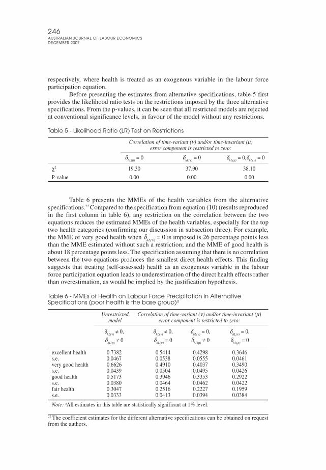
Before presenting the estimates from alternative specifications, table 5 firstprovides the likelihood ratio tests on the restrictions imposed by the three alternativespecifications. From the p-values, it can be seen that all restricted models are rejectedat conventional significance levels, in favour of the model without any restrictions.

Table 5 - Likelihood Ratio (LR) Test on Restrictions

Correlation of time-variant (ν) and/or time-invariant (µ)error component is restricted to zero:

δhL(µ)

= 0 δhL(ν)

= 0 δhL(µ)

= 0,δhL(ν)

= 0

χ2 19.30 37.90 38.10

P-value 0.00 0.00 0.00

Table 6 presents the MMEs of the health variables from the alternativespecifications.22 Compared to the specification from equation (10) (results reproducedin the first column in table 6), any restriction on the correlation between the twoequations reduces the estimated MMEs of the health variables, especially for the toptwo health categories (confirming our discussion in subsection three). For example,the MME of very good health when δ

hL(ν) = 0 is imposed is 26 percentage points less

than the MME estimated without such a restriction; and the MME of good health isabout 18 percentage points less. The specification assuming that there is no correlationbetween the two equations produces the smallest direct health effects. This findingsuggests that treating (self-assessed) health as an exogenous variable in the labourforce participation equation leads to underestimation of the direct health effects ratherthan overestimation, as would be implied by the justification hypothesis.

Table 6 - MMEs of Health on Labour Force Precipitation in AlternativeSpecifications (poor health is the base group)a

Unrestricted Correlation of time-variant (ν) and/or time-invariant (µ)model error component is restricted to zero:

δhL(ν)

≠ 0, δhL(ν)

≠ 0, δhL(ν)

= 0, δhL(ν)

= 0,

δhL(µ)

≠ 0 δhL(µ)

= 0 δhL(µ)

≠ 0 δhL(µ)

= 0

excellent health 0.7382 0.5414 0.4298 0.3646s.e. 0.0467 0.0538 0.0555 0.0461very good health 0.6626 0.4910 0.4037 0.3490s.e. 0.0439 0.0504 0.0495 0.0426good health 0.5173 0.3946 0.3353 0.2922s.e. 0.0380 0.0464 0.0462 0.0422fair health 0.3047 0.2516 0.2227 0.1959s.e. 0.0333 0.0413 0.0394 0.0384

Note: aAll estimates in this table are statistically significant at 1% level.

22 The coefficient estimates for the different alternative specifications can be obtained on requestfrom the authors.



The marginal effects in table 6 are based on the assumption that one can changehealth exogenously, without a change in the associated correlated unobservedheterogeneity terms of health and labour force participation. That is, health changesdue to a change in the exogenous factors in the health equation (of course someexogenous factors also affect labour force participation directly, in which case the neteffect may be different from the direct effect of health). If the change in health level isdue to one of the unobserved factors, the correlation between the two equations shouldbe taken into account to calculate the net effect. Given the relatively large negativeestimates for δ

hL(µ) and δ

hL(ν), this is expected to make a substantial difference. Table 7

presents the predicted probability of labour force participation conditional on the healthstatus. This accounts for the correlation of the unobserved terms. The reportedconditional probabilities are averages over the sample. Comparing the predictedconditional probability of people at different health levels in the lower section of table7, it can be seen that the implied effect of health is lower than that in table 6. Inaddition, comparing the most restricted specification in the last column with the leastrestricted specification in the first column, the effect of health on labour forceparticipation is smaller in the least restricted specification. The difference between theresults in tables 6 and 7 lies in the inclusion of time-variant and time-invariantunobserved terms that are negatively correlated across the two equations. Nevertheless,the effect of health on labour force participation remains substantial even when theindirect effect from unobserved variables is taken into account.

Table 7 - Predicted Conditional Probability of Labour Force Participation

Unrestricted Correlation of time-variant (ν) and/or time-invariant (µ)model error component is restricted to zero:

δhL(ν)

≠ 0, δhL(ν)

≠ 0, δhL(ν)

= 0, δhL(ν)

= 0,

δhL(µ)

≠ 0 δhL(µ)

= 0 δhL(µ)

≠ 0 δhL(µ)

= 0

Predicted conditional probability of participationPoor health 0.57 0.45 0.49 0.45Fair health 0.70 0.65 0.67 0.65Good health 0.74 0.74 0.75 0.75Very good health 0.77 0.81 0.79 0.80Excellent health 0.77 0.83 0.80 0.82

Compared to poorFair health 0.13 0.20 0.18 0.20Good health 0.17 0.29 0.26 0.29Very good health 0.20 0.35 0.30 0.35Excellent health 0.20 0.38 0.31 0.36

6. ConclusionThis paper examines the health effects on labour force status of older working-ageAustralian men. We use a random-effect approach to exploit the panel data nature ofthe HILDA survey and to control for unobserved heterogeneity. In addition, we controlfor the endogeneity of health, arising from unobserved heterogeneity, by introducinga health equation and allowing the error terms in the health equation and the labourforce status equation to be correlated.


The results show that the model estimated in the paper provides efficiencygains because all variance-covariance parameters of the error terms are found to besignificant. Restricting some of these parameters to zero would have reduced theefficiency of the estimates.

The estimates confirm the finding in the literature that health has a significantand large effect on labour supply. By comparing the different specifications of thecorrelation between the two equations, we find that any restriction on the correlationleads to an underestimation of the direct health effects. In particular, treating health asan exogenous variable, that is, to assume that the two equations are uncorrelated, isshown to lead to substantial underestimation of the direct health effects. This is aresult similar to Au et al. (2005). However, while Au et al. focused on the justificationbias and measurement error that could arise from using self-reported health, we focuson the potential correlation between unobserved factors affecting health and labourforce participation. Au et al., estimating different specifications of the employmentequation, found that using self-reported health leads to smaller estimated effectscompared to using a more objective health measure or including more objective healthconditions in other ways. From this they conclude that justification bias is unlikely tobe an issue and they attribute the underestimation from using self-reported health tomeasurement error. Our results suggest that underestimation could also result fromnot accounting for correlated unobserved heterogeneity. Of course, each explanationcould address part of the underestimation.

From a policy point of view, it is important to know the magnitude of healtheffects, because it can be used to estimate the indirect costs of a reduction in laboursupply caused by health problems. The results presented in this paper show that thecosts of health problems may be underestimated when using models that treat healthas an exogenous variable in the labour force status equation, compared with modelsthat account for the endogeneity of the health variable, such as the one used in thispaper. The larger costs of health problems estimated from a more efficient model maylend support to investment in policies aimed at improving health, especially olderworkers’ health. For example, programs that improve population health, in particularthe health of older workers, could be introduced to prevent potential labour shortagesarising from population ageing. In addition, policies encouraging workplace changesthat facilitate employment of staff with health problems are also likely to be important,particularly in the short run, in order to keep those older (and younger) workers, whoalready have health problems, in the labour force.



AppendixTable A1 - Descriptive Statistics of the Sample

Wave 1 Wave 2 Wave 3 Wave 1 to 3

Mean Std.Dev Mean Std.Dev Mean Std.Dev Mean Std.Dev

labour force 0.75 0.43 0.73 0.45 0.70 0.46 0.73 0.45health 2.28 1.05 2.19 1.0 2.16 1.02 2.21 1.03excellent health 0.11 0.31 0.09 0.28 0.08 0.27 0.09 0.29very good health 0.34 0.47 0.32 0.47 0.31 0.46 0.32 0.47good health 0.33 0.47 0.34 0.47 0.36 0.48 0.35 0.48fair health 0.16 0.36 0.20 0.40 0.19 0.39 0.18 0.38poor health 0.06 0.24 0.05 0.23 0.06 0.24 0.06 0.24age 55.7 3.7 56.6 3.7 57.6 3.7 56.6 3.8married 0.81 0.39 0.82 0.39 0.82 0.39 0.82 0.39child 0-14 0.13 0.34 0.11 0.31 0.10 0.30 0.11 0.32married*child 0-14 0.11 0.32 0.09 0.29 0.08 0.27 0.10 0.29born overseas 0.30 0.46 0.30 0.46 0.30 0.46 0.30 0.46born non-En country 0.13 0.34 0.13 0.34 0.13 0.34 0.13 0.34poor English 0.004 0.062 0.004 0.062 0.006 0.079 0.005 0.068indigenous 0.01 0.11 0.01 0.11 0.01 0.11 0.01 0.11degree 0.20 0.40 0.20 0.40 0.20 0.40 0.20 0.40other post-sch qual. 0.42 0.49 0.42 0.49 0.43 0.49 0.42 0.49completed year 12 0.07 0.25 0.07 0.25 0.06 0.25 0.07 0.25year 11 or lower 0.31 0.46 0.31 0.46 0.30 0.46 0.31 0.46white collar 1 0.35 0.48 0.34 0.48 0.34 0.48 0.34 0.48white collar 2 0.30 0.46 0.30 0.46 0.31 0.46 0.30 0.46blue collar 0.35 0.48 0.36 0.48 0.36 0.48 0.36 0.48smoker 0.63 0.48 0.65 0.48 0.66 0.47 0.65 0.48health condition 0.35 0.48 0.33 0.47 0.41 0.49 0.36 0.48heavy drinker 0.05 0.21 0.06 0.24 0.06 0.24 0.05 0.23lack of physical activity 0.13 0.34 0.14 0.34 0.14 0.35 0.14 0.34physical functioning 79.4 24.5 79.2 23.8 78.1 24.7 78.9 24.3living in capital city 0.53 0.50 0.53 0.50 0.54 0.50 0.53 0.50employment history 36.48 6.16 37.21 6.22 37.90 6.29 37.20 6.25unemployment history 0.55 1.94 0.60 2.01 0.63 2.06 0.59 2.00spouse in LF 0.53 0.50 0.48 0.50 0.47 0.50 0.49 0.50spouse income 1620 2244 1820 3100 1870 3603 1770 3035own NL income 344 1707 552 2448 755 4082 550 2923

number of observations 788 788 788 2364


Table A2 - Transitions in Health Status (row percentage)

Poor Fair Good Very Good Excellent Total

A. Year by year transitionsPoor 63.04 33.70 2.17 1.09 0.00 100Fair 8.96 61.29 25.81 3.94 0.00 100Good 0.38 15.63 60.26 22.22 1.51 100Very good 1.16 3.29 29.40 58.61 7.54 100Excellent 0.00 0.00 6.37 39.49 54.14 100

B. Transitions from year 1 to year 3Poor 55.10 42.86 2.04 0.00 0.00 100Fair 12.10 57.26 25.81 4.84 0.00 100Good 1.53 14.94 58.62 24.14 0.77 100Very good 0.37 5.24 34.08 53.93 6.37 100Excellent 1.15 2.30 10.34 36.78 49.43 100

Table A3 - Estimated MME Effects Using Alternative Health Categories as theBase

Base Health Category

Health Status Compared to Base Fair Good Very Good

Excellent 0.4334 *** 0.2209 *** 0.0756 ***(0.0427)a (0.0261) (0.0152)

Very good 0.3578 *** 0.1453 ***(0.0389) (0.0230)

Good 0.2126 ***(0.0292)

Note: aStandard errors are in parenthesis.

ReferencesAnderson, K.H. and Burkhauser, R.V. (1984), ‘The Importance of the Measure of

Health in Empirical Estimates of the Labour Supply of Older Men’, EconomicsLetter, 16, 375-380.

Anderson, K.H. and Burkhauser, R.V. (1985), ‘The Retirement-Health Nexus: A NewMeasure of an Old Puzzle’, Journal of Human Resources, 20, 321-330.

Au, D.W.H., Crossley, T.F. and Schellhorn, M. (2005), ‘The Effect of Health Changesand Long-Term Health on the Work Activity of Older Canadians’, HealthEconomics, 14, 999-1018.

Australian Bureau of Statistics (1998), Disability, Ageing and Carers Survey, ABScatalogue 4430.0.

Barsky, R.B., Juster, F.T., Kimball, M.S. and Shapiro, M.D. (1997), ‘PreferenceParameters and Behavioral Heterogeneity: An Experimental Approach in theHealth and Retirement Study’, Quarterly Journal of Economics, May, 537-579.

Bazzoli, G.J. (1985). ‘The Early Retirement Decision: New Empirical Evidence onthe Influence of Health’, Journal of Human Resources, 20, 214-234.

Benitez-Silva, H., Buchinsky, M., Chan, H.M., Cheidvasser, S. and Rust, J. (2004),‘How Large is the Bias in Self-assessed Disability?’ Journal of AppliedEconometrics, 19, 649-670.



Blau, D.M. and Riphahn, R.T. (1999), ‘Labor Force Transitions of Older MarriedCouples in Germany’, Labour Economics, 6, 229-251.

Boaz, R.F. and Muller, C.F. (1990), ‘The Validity of Health Limitations as a Reasonfor Deciding to Retire’, Health Services Research, 25, 361-386.

Börsch-Supan, A. and Hajivassiliou, V.A. (1993), ‘Smooth Unbiased MultivariateProbability Simulators for Maximum Likelihood Estimation of LimitedDependent Variable Models’, Journal of Econometrics, 58, 347-368.

Bound, J. (1991), ‘Self-assessed Versus Objective Measures of Health in RetirementModels’, Journal of Human Resources, 26, 106-138.

Bound, J., Schoenbaum, M. and Waidmann, T. (1995), ‘Race and Education Differencesin Disability Status and Labor Force Attachment in the Health and RetirementSurvey’, Journal of Human Resources, 30 (Supplement), S227S267.

Cai, L. and Gregory, R.G. (2003), ‘Inflows, Outflows and the Growth of theDisability Support Pension (DSP) Program’, Australian Social Policy 2002-03, 121-143.

Cai, L. and Kalb, G. (2006), ‘Health Status and Labour Force Participation: Evidencefrom Australia’, Health Economics, 15, 241-261.

Campolieti, M. (2002), ‘Disability and the Labor Force Participation of Older Men inCanada’, Labour Economics 9, 405-432.

Chirikos, T.N. (1993), ‘The Relationship between Health and Labor Market Status’,Annual Reviews of Public Health, 14, 293-312.

Currie, J. and Madrian, B.C. (1999), ‘Health, Health Insurance and the Labor Market’,in Ashenfelter, O. and Card, D. (eds.), Handbook of Labor Economics, ElsevierScience Publisher.

Disney, R., Emmerson, C. and Wakefield, M. (2006), ‘Ill Health and Retirement inBritain: A Panel Data-Based Analysis’, Journal of Health Economics, 25, 621-649.

Dwyer, D.S. and Mitchell, O.S. (1999), ‘Health Problems as Determinants ofRetirement: Are Self-Rated Measures Endogenous?’ Journal of HealthEconomics, 18, 173-193.

Ferraro, K.F. (1980), ‘Self-Ratings of Health among the Old and Old-Old’, Journal ofHealth and Social Behavior, 21, 377-383.

Gerdtham, U.G., Johannesson, M., Lundberg, L. and Isacson, D. (1999), ‘A Note onValidating Wagstaff and van Doorslaer’s Health Measure in the Analysis ofInequality in Health’, Journal of Health Economics 18, 117-224.

Gray, M.C., Hunter, B.H. and Taylor, J. (2003), ‘Health Expenditure, Income andHealth Status among Indigenous and Other Australians’, in Anderson, I. (ed.),The Economics of Indigenous Health, University of Melbourne Press,Melbourne.

Greene, W.H. (1993), Econometric Analysis (2nd Edition), New York: MacmillanPublishing Company.

Grossman, M. (1999), ‘The Human Capital Model of the Demand for Health’, inNewhouse, J. P. and Culyer, A. J. (eds.), Handbook of Health Economics, North-Holland, Amsterdam.

Hajivassiliou, V. (2000), ‘Some Practical Issues in Maximum Simulated Likelihood’,inMariano, R., Schuermann, T. and Weeks, M.J. (eds.), Simulation-Based Inferencein Econometrics: Methods and Applications, Cambridge University Press.


Hajivassiliou, V. and Ruud, P. (1994), ‘Classical Estimation Methods for LDV ModelsUsing Simulation’, in Engle, R. and McFadden, D. (eds.), Handbook ofEconometrics, Vol. 4, Elsevier Science Publishers, Amsterdam.

Hsiao, C. (2003), Analysis of Panel Data (2nd Edition), Cambridge University Press.Hyslop, D.R. (1999), ‘State Dependence, Serial Correlation and Heterogeneity in

Intertemporal Labor Force Participation of Married Women’, Econometrica,67, 1255-1294.

Idler, E.L. and Kasl, S.V. (1995), ‘Self-Ratings of Health: Do They Also Predict Changein Functional Ability?’ Journal of Gerontology, 50B, 344-353.

Jin, R.L., Shah, C.P. and Svoboda, T.J. (1995), ‘The Impact of Unemployment onHealth: A Review of the Evidence’, Canadian Medical Association Journal,153, 529-540.

Kreider, B. (1999), ‘Latent Work Disability and Reporting Bias’, Journal of HumanResources, 34, 734-769.

Maddala, G. (1983), Limited Dependent and Qualitative Variables in Econometrics,Cambridge University Press, New York.

McCallum, J. Shadbolt, B. and Wang, D. (1994), ‘Self-Rated Health and Survival: A7-year Follow-up Study of Australian Elderly’, American Journal of PublicHealth, 847, 1100-1105.

Melbourne Institute of Applied Economic and Social Research (2005), ‘Household,Income and Labour Dynamics in Australia (HILDA) Survey Annual Report2004’, University of Melbourne.

Sickles, R. and Taubman, P. (1986), ‘An Analysis of the Health and Retirement Statusof the Elderly’, Econometrica, 54, 1339-1356.

Stern, S. (1989), ‘Measuring the Effect of Disability on Labour Force Participation’,Journal of Human Resources, 24, 361-395.

Stern, S. (1997), ‘Simulation Based Estimation’, Journal of Economic Literature, 35,2006-2039.

Wagstaff, A. and van Doorslaer, E. (1994), ‘Measuring Inequalities in Health in thePresence of Multiple Category Morbidity Indicators’, Health Economics, 3,281-291.

Ware, J., Snow, K., Kosinski, M. and Gandek, B. (2000), SF-36 Health Survey: Manualand Interpretation Guide, Lincoln, RI, Quality Metric Incorporated.

Watson, N. and Wooden, M. (2002), ‘The Household, Income and Labour Dynamicsin Australia (HILDA) Survey: Wave 1 Survey Methodology’, HILDA ProjectTechnical Paper Series No. 1/02. Melbourne Institute of Applied Economicsand Social Research, the University of Melbourne.

Wilkins, R. (2004), ‘The Effects of Disability on Labour Force Status in Australia’,Australian Economic Review, 37, 359-382.

Wilson, C.M. and Oswald, A.J. (2005), ‘How Does Marriage Affect Physical andPsychological Health? A Survey of the Longitudinal Evidence’, IZA DiscussionPaper No. 1619.

Zhang, X., Zhao, X. and Harris, A. (2006), ‘Chronic Illnesses and Labour ForceParticipation in Australia’, paper presented at the Australian Health EconomistsSociety Conference, Perth, 28-29 September.

Health Status and Labour Force Status of Older Working-Age...

Documents

Transcript of Health Status and Labour Force Status of Older Working-Age...