Have Filipino Households Become Less Prudent? Akiko · PDF fileHave Filipino Households Become...

1

Have Filipino Households Become Less Prudent?

Akiko Terada-Hagiwara

November 4, 2010

June 9, 2011

This version: September 9, 2011

Abstract

Throughout the 2000s, the average household saving rate in the Philippines declined

sharply. This paper explains why households' consumption growth has been higher than

income growth during this period. Tracing cohorts shows that saving declined across all

demographic groups. A test that provides the strength of the precautionary saving

motive yields a plausible explanation that households have become financially

constrained and less prudent in the recent years. This paper argues that these patterns

are best explained by the extended coverage of social security system particularly to

informal sector employees during the 1990s in the Philippines.

Asian Development Bank; 6 ADB Avenue, Mandaluyong City 1550, Philippines; Tel (632) 632 5587, Fax (632)

636 2342; [email protected].

This paper has benefited from comments from seminar participants at the Institute of Social and Economic Research, Osaka University and 12th International Convention of the East Asian Economic Association, Korea. The author appreciates the help of Charles Y. Horioka, Eswar Prasad, and Shikha Jha for useful discussions at different stages of the paper, and Shiela Caming, Aleli Rosario and Pilipinas Quising for capable research assistance. However, the author is solely responsible for any remaining errors.

mailto:[email protected]

2

I. Introduction

From 1994 to 2006, the average household saving rate in the Philippines declined

by 5.2 percentage points to about mere 5% of disposable income. The Philippines

provides an excellent laboratory to study the determinants of household saving for

its dynamic developments in determining factors over the decade.

First, real GDP growth rate had undergone a transition from relatively steady growth

in the 1960s and 1970s to sharp fluctuations in the 1980s and 1990s. The older

cohorts enjoyed higher and steadier economic growth, while those relatively younger

cohorts lived under relatively volatile economic situation. The second feature of the

Philippines that is relevant to life-cycle saving is its demographic change over the

last several decades. The age distribution of the population has been sharply

skewed toward the younger population. Third, the nation’s social security system

had evolved quite rapidly during the 1990s, which would affect the consumption and

saving behavior significantly. An evolving social security system, stagnant economic

growth, declining yet still high population growth, and fertility rate all have

consequences for saving rate.

This paper contributes to the literature by arguing that the usual suspects—rising

youth dependency and stagnant income growth—are not sufficient to explain the

observed declining trend in the Philippines as suggested such as by Bersales and

Mapa (2006). This paper is the first to show that the declining saving rate has been

3

due to the reduced precautionary motives as partly expected by developments such

as the expansion of the social security system. More extensive coverage of the

system to the informal sector employees appears to have reduced households’

precautionary savings, which has been magnified by the slow income growth.

In order to arrive at this conclusion, we first show that the declining trend remains

even after controlling for the demographic variables. Also, the declining trend cannot

be simply due to the aggregate macroeconomic shocks as suspected. Liquidity

constraint and precautionary behavior are then considered to show how they affect

saving rates of Filipino households over time. Additionally, this paper finds that the

Filipino age–saving rate profile fits in the standard life cycle hypothesis showing a

hump-shaped age–saving rate profile, once controlled for the demographic shifts

and family composition.

The paper is organized as follows. Section II describes the survey data and provides

some stylized facts on the saving behaviors of Filipino households. Section III

adapts a decomposition analysis to argue that the demographic changes are not

sufficient to explain the declining saving rate. In Section IV, we introduce uncertainty

in consumption to test for precautionary motives. Changing precautionary motives

would explain the downward time-saving rate profile. The final section concludes.

II. The Survey Data and Stylized Facts

4

A. The Survey Data

We use household income and expenditure surveys (FIES)—from 1988 through

2009. In the Philippines, FIES is conducted every three years, and a total of eight

survey results are available over this period.i We measure saving as the difference

between disposable income and total (and non-durable) consumption expenditures.

The measure of disposable income that we focus on includes agricultural and non-

agricultural salaries and wages from regular employment, net share of crops, cash

receipts, and other assistance from both overseas and domestic sources. Interest,

pension and social security benefits, and dividends from investment are also

included. Taxes are excluded.ii

B. Puzzle on Declining Household Saving Rate

Demographic development has been cited as one of the factors to explain the

declining saving trend in the Philippines.iii The increase in the young dependency

group would have increased the education and health expenditures, which could

result in lower aggregate saving.

For most of the interesting questions about saving and the life cycle, it is necessary

to track individuals over time, and to observe the changes in consumption, income,

and saving as people age. Although we cannot track individual households in the

data, we can track cohorts of households, with cohorts defined according to their

year of birth. With the FIES data, we can follow cohort means for 1988 to 2009.

5

Figure 1 shows how the cohort grouping can be used to show both the life cycle

pattern of family formation and the cohort effects of increasing fertility. The age of

the head of the household is plotted on the horizontal axis, while the vertical axis

shows the average number of children in the household. Children here are defined

those under age 25. The plotted points are connected when we follow the same

cohort through time, but different cohorts are left unconnected. To avoid clutter, we

show only every tenth cohort, so that the first segment on the left hand side of the

figure shows the number of children in households headed by those who were 25 in

1965. By the time these people are 35 in 1975, they are well launched into their

child-bearing years, and have 3.5 children on average. The peak comes when the

heads’ age is about mid-40s with about 4.5 children on average. The falling fertility

shows up in the profiles as we move from one cohort to the next.

<Insert Figure 1 here>

To gauge the time series characteristics of the household saving behavior, Figure 2

plots income and consumption against the age of the household head, with each

panel corresponding to a different cohort. Many cohorts experienced a sharp

increase and drop in income and consumption—the observation shared across

different cohorts. Most notably, those cohorts of 1960 or later are found to save

much less than older cohorts regardless of their age. This finding suggests an

importance of time effects in consumption and saving behaviors. In the next section,

we will show that controlling for demographic effects do not provide an answer to the

6

declining saving rate.


III. Controlling for Demographic Effects on Household Saving Rates: A

Decomposition Analysis

The Philippines, like many other countries, is undergoing a major demographic

transition. Hence, a careful analysis of demographic factors seems warranted in

accounting for the observed saving behavior. Moreover, different age and cohort

groups are likely to have very different saving behavior and these are likely to

change. It is therefore necessary to separate age, cohort, and time effects to more

clearly characterize the effects of demographic variation on changes in saving

patterns.

A. Decomposition Methodology

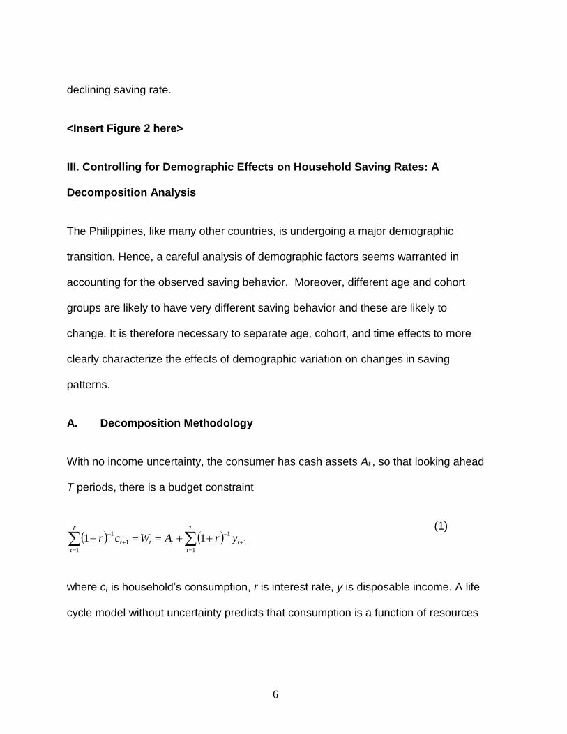
With no income uncertainty, the consumer has cash assets At , so that looking ahead

T periods, there is a budget constraint

T

t

ttt

T

t

t yrAWcr1

1

1

1

1

111

(1)

where ct is household’s consumption, r is interest rate, y is disposable income. A life

cycle model without uncertainty predicts that consumption is a function of resources

7

(earnings plus inherited assets), with the constant of proportionality depending on

the household head and the real interest rate. Given 1/T is a function of age, the

consumption can be expressed as follows:

hhha Wafc

where cha denotes the consumption of household h headed by an individual of age a

and with lifetime resources Wh. This equation holds at the level of the individual, but

given its additive structure, after taking logs, it can be averaged over all households

of the same age as defined by the head’s age in each year, t, which yields the

following expression.

bat Wafc lnlnln

This treatment allows us to decompose into a wealth term, which is regarded

constant within cohorts, and an age term. The age effects afln are captured by a

vector of age dummies, and the lifetime resources bWln by a vector of cohort (year

of birth) and time dummies. Deaton and Paxson (1994) considered additional time

effects to account for the presence of macroeconomic effects, which cannot be

explained by cohort or age effects. The life cycle model with uncertainty provides

some basis to have time effects once uncertainty is admitted as wealth levels will be

revised in response to macroeconomic shocks. The issue of uncertainty is looked at

more closely in the next section. A decomposition follows a simple formula as

8

follows:

cc

t

c

b

c

a

at DDDc ln (2)

where Da, D

b, and D

t are matrices of age, year of birth, and year dummies,

c ,c,

andcare the corresponding age, cohort, and year effects on consumption, and

c is

the error term.iv v

Following equation (1), income is similarly estimated using an equation analogous to

the one for consumption.vi

yy

t

y

b

y

a

at DDDy ln (3)

where Da, D

b, and D

t are matrices of age, year of birth, and year dummies as in

equation (2), y ,

y, and

yare the corresponding age, cohort, and year effects on

income, and y is the error term. Saving ratio is measured based on the estimated

equations as the difference of the logarithms of income and consumption, or the

equation (2)-(3).

B. Decomposition Results

Figure 3 show the estimated age, cohort, and time profiles of income, consumption,

and saving rates. When estimating these equations, we also include demographic

9

controls, such as log (family size), log (employed members), and the share of

individuals in the household aged 1–6, 7–14, 15–24, and 25 and above.vii

The age effects show that the saving rate starts to fall slightly earlier than the

standard retirement age of sixty in the Philippines unlike the monotonically

increasing saving rate with age that the unconditional mean suggests.viii

This result

can be attributed to the controls that are included—the share of different age family

members. The age-saving profile becomes hump-shaped as shown in Figure 3. The

saving rate reaches its peak at the household head’s age of about mid-50s, and its

trough before the head reaches age 30 and again close to age 70. This result

suggests that saving rate is lowest when household heads’ age is about 40 because

the children’s education and associated costs are highest around this time.ix

The cohort profile of income, consumption, and saving suggest that younger and

older cohorts had relatively higher income than those who were in their mid-50s in

1988. The resulting effect on savings suggests that the higher saving cohorts are

older cohorts—those that were in their mid-60s in 1988—saving about 2–3

percentage points more than earlier cohorts, which may be capturing the fact that

those cohorts were unscathed by the economic downturns of the early 1980s and

late 1990s.

Finally, we turn to the time profile. The time effects explain more than 7 percentage

points decrease in the saving rate from 1988 to 2009. Given the fact that

10

demographic characteristics are already controlled for, this is a significant number

suggesting a limited role for demographic changes in explaining the decline in

Filipino household savings over the last two decades. This result is robust to

alternative definition of the saving rate such as total household income minus total

household expenditure that Bersales and Mapa (2006) uses.

Either aggregate macroeconomic or institutional shifts explain the declining saving

rate. One factor might be a higher inflation rate in the 2000s driven mainly by a hike

in oil and food prices, and/or negative real interest rate. Alternatively, the saving

behavior might have been affected by a shift in a precautionary motive of Filipino

households, as also suggested from the cohort effects. These uncertainty and time

series factors are investigated further in the next section.


IV. Precautionary Motive with Uncertainty in Consumption

Given the importance of the uncertainty as suggested in the previous sections,

theories of precautionary saving have intuitive appeal and important implications.

Deaton (1992) emphasizes that uncertainty may substantially alter consumers’

behavior.x Since demographic shifts do not seem to be able to account for the

decline in household saving rate with time, we now discuss an alternative hypothesis

that could account for the declining time–saving rate profile. As suggested in the

11

previous section, we investigate if there has been a role in the precautionary motive

in the Filipino households and how macroeconomic developments affected the

behavior. One would expect a declining saving rate over time if the household

saving behavior has been less prudent in the recent years.

A number of factors are relevant in affecting the precautionary motive of the Filipino

households. First, the Philippines’ Social Security System developed significantly

during the 1990s. Existing studies found that coverage by social programs, such as

disability insurance, unemployment insurance, and health insurance, is negatively

associated with saving. In fact, the coverage of the system, which covers

contingencies such as disability, health, and old age, had been extended

intensively.xi In 1988, only less than half of the Filipino workers were covered in the

system. After the coverage was extended to include non-working spouses, self-

employed workers and agricultural workers in the 1990s, the system now covers 3

out of every 4 workers. Household helpers and informal sector workers who earn at

least 1,000 pesos a month were also included by mid-1990s. This expanded

coverage of the social security system implies a reduced need for younger cohorts

to accumulate precautionary savings.

That saving provides insurance for future contingencies has long been recognized in

literature, but this precautionary motive has played a minor role in the empirical

investigation of the household saving behavior in general, and Filipino households in

particular.xii

Because of the significant development such as in the social security

12

system in the Philippines, we estimate relative prudence considering the liquidity

constraints in this section.

A. Estimation Methodology

The empirical framework follows Zeldes (1989), where the Lagrange multiplier

associated with the liquidity constraint is added to the consumption Euler equation.

,'1

1' ,1,, tititti cUE

rcU

where Et is the conditional expectation operator, is the

Lagrange multiplier associated with the liquidity constraint. This condition shows that

greater uncertainty is linked to greater saving when the third derivative of utility is

positive. An increase in uncertainty raises the expected variance of consumption,

which in turn implies higher expected marginal utility when marginal utility is convex.

Taking the second-order Taylor approximation of 1,' tit cUE around tic , yields the

consumption growth equation as follows.

,~

21

1,

2

,

,1,

,

,1,

ti

ti

titi

t

ti

titi

tc

ccE

r

r

c

ccE

(4)

where is the coefficient of relative risk aversion, '

'' ,

U

cU ti ; is the coefficient of

13

relative prudence, ''

''' ,

U

cU ti ; and

''1

1~

,

,

,Ucr ti

ti

ti

. 0

~ for the liquidity-

constrained households in equation (4). If

consumption growth (which reflects higher saving) is associated with higher

expected squared consumption.xiii

Having panel data to test this hypothesis is ideal—however, FIES does not provide

the panel data. We therefore follow Deaton (1985) to form time series data from the

cross sectional data that we examine from the FIES. Corresponding to individual

behavior, a cohort version of the relationship of the same form exists, but ―with

cohort‖ means replacing individual observations. We eliminate the cohorts that do

not exist for all eight surveys (1988–2009). As a result, the sample of this section

has 25 cohorts from 11 regions in the Philippines. Those cohorts include the heads

who were born from 1939 to 1963.xiv

We restrict the sample to households whose

head is 25–70 years old. Again, each observation in this regression is weighted by

the square root of the number of original observations that its average is based on.

Figure 4 shows box plots of the squared consumption growth by year. The degree of

dispersion and median value of the squared consumption growth—uncertainty

measure—have been reduced steadily over time as we expect. A notable exception

is 1997 possibly affected by the Asian financial crisis.

Estimation specification uses an initial income as a proxy for ~

.

14

,11

0,2

2

1 ,

,1,

10

1 ,

,1,

ii

N

t ti

titiN

t ti

titi yc

cc

Nc

cc

N

(5)

where

r

r

1

10

,

21

, N represents the number of periods, yi,0 is the initial

income, and i is the expectation error. The size of determines the strength of

the precautionary saving motive. We expect 02 for the constrained and 02

for the unconstrained. We use the instrumental variable technique. Squared

consumption growth, which is a proxy variable for uncertainty, is instrumented with

the household head’s education and share of income from agriculture sector.

Income growth and demographic variables, i.e. share of individuals in the household

aged 1–6, 7–14, 15–24, and 25 and above are also included. Cohort dummy

variables enter as a taste shifter, and macroeconomic developments are controlled

by real interest rate.xv

The uncertainty variable is Interacted with various variables

such as dummy variables for different sub-periods, household heads’ job category,

and income group, and included in regressions one by one to examine if each sub-

group and/or -period has additional effects on the consumption growth and hence

the saving rate.

B. Estimation Results

Table 1 columns A to C show results of instrumental variable estimation with and

without the interacted variables with sub-period dummies. The results are interesting

15

and intuitive suggesting an important role played by the precautionary motive in the

Filipino households’ consumption behavior. The first stage results are shown in the

lower part of the columns for all the estimation results, and generally plausible.

Engoneniety test results suggest that the instrumental variable estimation is

consistent while the underidentification test results indicate that the equations are

identified. Test for weak instruments is also conducted. The Wald F statistics

suggest that the null hypothesis of weak instruments can be mostly rejected at 10%,

B.1. Estimation Results: overall vs 2000s

The estimated coefficients on the squared consumption growth for the entire sample

reveal that risk affects consumption positively and significantly. The estimation result

for the entire sample in the column A shows a significant role played by the

uncertainty with its coefficient being 2.03 and significant on the consumption growth.

This is what precautionary hypothesis predicts: households that face more risks

save more. The estimated strength of the precautionary motive also appears to be

significant and plausible in magnitude.xvi

Since income growth and demographic

variables are also controlled for, this result contributes to the literature by arguing

that the usual suspects—rising youth dependency and stagnant income growth—are

not sufficient to explain the observed declining trend in the Philippines as widely

suggested in the existing literature.

The interactive variable with the dummy for the 2000s is then included to investigate

16

if there has been a shift in precautionary motive in Filipino households. The results

are interesting and intuitive. This precautionary motive disappeared in the 2000s as

shown in the columns B and C, which include the interactive variables with sub-

sample dummies for the 2000s and the years after 2003. The estimated coefficients

on the interacted variables are significant and negative in both cases leading the net

effects of the uncertainty variable to be insignificantly different from zero showing no

sign of prudence.

Our empirical results are consistent with studies that have found that coverage by

social programs, such as disability insurance (Kantor and Fishback, 1996),

unemployment insurance (Engen and Gruber, 2001), and Medicaid (Gruber and

Yelowitz, 1999) in the US, and health insurance (Chou et al, 2003) in Taipei,China,

are negatively associated with saving.

<Insert Table 1 here>

B.2. Estimation Results: overall vs households with informal sector jobs

In the next stage, we examine if this changing behavior in the 2000s is associated

with the extended coverage of the social security system to informal sector workers.

The informal sector jobs are defined as those the Social Security System was

extended during the 1990s, which include self employed workers, workers in private

households, and employers and employees of own family-operated farms and

businesses. Households that are categorized to have the informal sector jobs

17

consist a half of the surveyed households.

Columns A, B, and C of Table 2 show the results including the interacted variables

for informal sector jobs. Interestingly, simply having an informal sector job would not

lead to become less prudent, and does not have significant additional impacts on the

consumption behavior. Households are generally prudent as reported in column A.

However, being in informal sector starts to matter in the 2000s with the significant

negative coefficient, -0.81, on the uncertainty variable as reported in column B. This

impact can be understood as a possible significant impact arising from the extended

Social Security System consistent with our prior.xvii

<Insert Table 2 here>

B.3. Estimation Results: Low versus High income

Further, we test the assumption of constant absolute prudence imposed in equation

(5) above— how low-income consumers react differently to the factors affecting the

uncertainty. Kimball (1990) suggests that prudence, like risk aversion, is likely to

decline with wealth suggesting that lower-income people will be more sensitive to

the risk reductions, that is, the wider coverage of social security system will have a

larger impact on their precautionary saving and consumption.

An estimation exercise is conducted including an interactive variable for the poor

households with informal sectors jobs in 2000s. The poor households are defined as

18

those below the median income. The estimation result in column C supports the

claim with the significantly negative coefficient, -1.67—much larger (in absolute

term) than that with all the income groups considered. When the definition of the

poor changed to those below income of 25% of the sample, the absolute value of the

coefficient (not reported) is even larger (-2.82).xviii

The result indicates that the

impact from the extension of social security system is particularly large for the lower

income households validating the claim made by Kimball (1990) among others.

Other variables included in the estimation exercise are generally consistent. The

estimated coefficients on the interest rate terms are negative consistent with the

prior that the higher interest rate slows consumption growth. Coefficient on income

growth is positive and significant in all cases validating its importance. The

contraction in the average household income in the 2000s has been contributing to

the slowing consumption growth. Although not reported here to save space, two of

the demographic variables significantly explain the consumption growth—positive for

the share of individuals in the household aged 1 and below. The coefficient on initial

income is mostly positive or insignificant while we expect that the coefficient to be

negative when households are financially constrained. This result is not affected

even when different wealth measure is included.xix

One possible reason for this

result is a habit formation, which implies that consumption reacts slowly to declining

income explaining the initial income affecting consumption growth positively.

V. Concluding Remarks

19

This paper explains why the average household saving rate in the Philippines

declined substantially in the 2000s. Contrary to what was generally believed, our

decomposition analysis suggests that demographic factors do not fully explain the

declining time-saving rate profile. On the other hand, we find that the declining

saving rate is associated with the changing precautionary motives of Filipino

households.

We find that the precautionary saving was strong in the 1990s when the coverage of

the social security system was still limited. However, the precautionary motive does

not seem to be present in the 2000s. The less prudent behaviors are found to be

significant with households with informal sector jobs, but only in the 2000s validating

the extended social security system being the major factor affecting the Filipino

households saving behavior. Moreover, this impact is found particularly strong with

lower income households in the 2000s. Our evidence supports the contention that

precautionary motives, particularly of low-income households, are an important

determinant of saving.

20

Endnotes

i The eight surveys were conducted consistently using the same survey and sampling designs. For

details, see Appendix 1 of Terada-Hagiwara (2009). ii The tax rate is slightly higher for high income households averaging at 1.4% (of total income) as

compared with 0.8% for relatively low income group. Though taxes can affect consumption behavior differently across different income groups, the results of our analyses are not affected by the definition used possibly due to the marginal difference in the tax rates. iiiBersales and Mapa (2006) analyze the same survey (up to 2003) and report that the declining trend

has to do with the higher proportion of young dependents in the economy. iv Each observation in this regression is weighted by the square root of the number of original

observations that its average is based on. To exclude unreliable observations, the observations are dropped when the number of original observations is less than 300 per each cohort. v Deaton and Paxson (1994) identify age and cohort effects by imposing a constraint that the year

effects must add up to zero and be orthogonal to a time trend. This constraint forces the decomposition to attribute the rising income and consumption to age and cohort effects, not to time. In the case of the Philippines, the country experienced macroeconomic fluctuations during the sample period, unlike Taipei,China as in Deaton and Paxson (1994), where positive GDP growth was steadily recorded during the period. Thus, it is more appropriate to identify time effect arising from the macroeconomic fluctuations by imposing constraint on the cohort effects in the case of the Philippines. viChamon and Prasad (2008) argue that to the extent the age profile of income is invariant to

economic growth, then income can also be expressed as a function of age and lifetime resources. vii

In this exercise, we take our baseline household as one whose head was 25 years old in 1988. For example, the age profile shows how income and consumption would vary with age, holding the cohort effect constant at the level for the cohort born in 1963 and the year effect at its 1988 level. Similarly, the cohort profile shows how income and consumption would vary with year of birth, holding constant the age effect at its level for 25-year olds and the year effect at its 1988 level. Finally, the year profile shows the variation over time holding constant the age effect at its level for 25-year olds and the cohort effect at the level of those born in 1963. viii

In fact, the flow of saving should not only decline after retirement but should become negative. This is not visible in this exercise since there are more than one employed members in the households with the age of the head beyond the normal retirement age of 60. See detailed discussion in Terada-Hagiwara (2009). ixThe result holds when we use non-durable consumption instead of the total expenditure.

xSkinner (1988) derives an approximation for optimal life cycle consumption that implies that, with

plausible amounts of income uncertainty and risk aversion, precautionary saving is more than half of total life cycle saving. xi As part of the Employees' Compensation Program in 1992, coverage was extended for self-

employed workers. In January 1992, compulsory coverage of self-employed farmers and fishermen earning at least P1,500 per month or P18,000 per annum was initiated. Later in the year, voluntary coverage was extended for non-working spouses of Social Security System members (RA 7192 – Women in Nation-Building Act). In 1993, compulsory coverage included household helpers earning at least P1,000 a month. In 1995, voluntary coverage was expanded to overseas contract workers and self-employed persons with a monthly net income of at least P1,000. In 1997, expanded compulsory coverage included self-employed workers and agricultural workers who are not paid any regular daily wage or who do not work an uninterrupted period of at least 6 months, household helpers, parents employed by children, and minors employed by parents. xii

Chou et al. (2003) provides a survey of past theoretical and empirical literature on the issue.

21

xiii

This condition holds for the constant risk aversion utility function and the constant absolute risk aversion function, but does not hold for quadratic utility, by which consumers’ utility is affected by the presence of uncertainty, but their behavior does not change in response to it. xiv

Durable expenditures are excluded from the analysis because they affect utility for more than one quarter, violating the assumption that utility is time separable. xv

A dummy variable for 1997, which would potentially capture the effects of Asian financial crisis, was also added. The coefficient on the dummy variable was insignificant and did not affect the results. The dummy variable was not included in the estimations reported in the paper. xvi

Mehra and Prescott (1985) cite a variety of studies that conclude that the coefficient of relative risk aversion is at least one, and their own analysis of the historical risk equity premium implies that the coefficient must be much larger than 10. The constant relative risk aversion (CRRA) utility would imply the size of prudence to vary between 2 and 5 corresponding to the coefficient ranging from 1 to 4. xvii

Manasan (2009) reports that only about 30% or 8 millions are contributing members as of total 27.2 million that are covered by the Social Security System. Despite the still limited share of contributing members, the expansion of the Social Security System to cover previously excluded population seemed to have a significant impact on their behavior— informal sector households are becoming less prudent over time, which is our focus. xviii

Comparable studies for developing countries are still limited, but the result is consistent with Chou et al. (2003), which shows that the absolute prudence of the lowest income quantile is almost twice as large as the one immediately above quantile. xix

The measure tried includes rental from non-agricultural lands, buildings, other properties, and interest from bank deposits and loans to other households.

References

Bersales, Lisa Grace and Dennis Mapa. 2006. Patterns and Determinants of

Household Saving In the Philippines. Report prepared under the EMERGE

Project of USAID. Available:

www.stat.upd.edu.ph/ARTICLES/Article3/Paper_BERSALES_MAPA.pdf.

Chamon, M. and E. Prasad. 2008. “Why Are Saving Rates of Urban Households in

China Rising.” NBER Working Paper 14546. National Bureau of Economic

Research. Cambridge, Massachusetts:

Chou, Shin-Yi, Jin-Tan Liu, and James K. Hammitt, 2003. “National Health Insurance

and precautionary saving: evidence from Taiwan.” Journal of Public Economics

87(2003): 1873–1894.

Deaton, Angus. 1985. “Panel Data from Time Series of Cross-Sections.” Journal of

Econometrics 30(1985): 109–126.

Deaton, Angus. 1992. “Understanding Consumption.” Clarendon Lectures in

Economics. New York: Oxford University Press Inc.

Deaton, Angus and Christiana Paxson. 1994. “Saving, Growth, and Aging in Taiwan.”

Studies in the Economics of Aging. National Bureau of Economic Research

Project Report Series. Chicago and London: University of Chicago Press.

Dynan, Karen. 1993. “How prudent are consumers?” Journal of Political Economy

101: 1104–1113.

Engen, E.M. and J. Gruber. 2001. “Unemployment insurance and precautionary

saving.” Journal of Monetary Economics 47 (3): 545–579.

Gruber, J. and A. Yelowitz. 1999. “Public health insurance and private savings.”

Journal of Political Economy 107 (6): 1249–1274.

Kantor, S.E. and P.V. Fishback. 1996. “Precautionary saving, insurance, and the

origins of workers compensation.” Journal of Political Economy 104 (2): 419–

442.

Kimball, Miles, 1990. “Precautionary Saving in the Small and in the Large,”

Econometrica 58, (1) (Jan., 1990): pp 53-73.

Manasan, Rosario G. 2009. “Social insurance in the Philippines: responding to the

global financial crisis and beyond.” Philippines Institute for Development Studies

Discussion Paper 2009-03. Manila.

Mehra, Rajnish, and Edward C. Prescott. “The Equity Premium: A Puzzle.” Journal of

Monetary Economics 15 (March 1985): 145–161.

Skinner, Jonathan. 1988. “Risky Income, Life Cycle Consumption, and Precautionary

Savings.” Journal of Monetary Economics 22 (September 1988): 237–255.

Terada-Hagiwara, A. 2009. “Explaining Filipino Households’ Declining Saving Rate.”

ADB Economics Working Paper Series, No. 178. Manila.

Zeldes, Stephen P. 1989. “Consumption and liquidity constraints: an empirical

investigation.” Journal of Political Economy 97: 305–346.

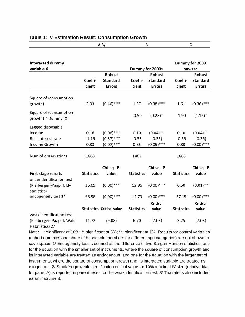
Table 1: IV Estimation Result: Consumption Growth

Interacted dummy

variable X

Coeffi-

cient

Robust

Standard

Errors

Coeffi-

cient

Robust

Standard

Errors

Coeffi-

cient

Robust

Standard

Errors

Square of (consumption

growth) 2.03 (0.46)*** 1.37 (0.38)*** 1.61 (0.36)***


growth) * Dummy (X)-0.50 (0.28)* -1.90 (1.16)*

Lagged disposable

income 0.16 (0.06)*** 0.10 (0.04)** 0.10 (0.04)**

Real interest rate -1.16 (0.37)*** -0.53 (0.35) -0.56 (0.36)

Income Growth 0.83 (0.07)*** 0.85 (0.05)*** 0.80 (0.00)***

Num of observations 1863 1863 1863

First stage results Statistics

Chi-sq P-

value Statistics

Chi-sq P-

value Statistics

Chi-sq P-

value

underidentification test

(Kleibergen-Paap rk LM

statistics)

25.09 (0.00)*** 12.96 (0.00)*** 6.50 (0.01)**

endogeneity test 1/ 68.58 (0.00)*** 14.73 (0.00)*** 27.15 (0.00)***

Statistics Critical value StatisticsCritical

value StatisticsCritical

value

weak identification test

(Kleibergen-Paap rk Wald

F statistics) 2/

11.72 (9.08) 6.70 (7.03) 3.25 (7.03)

Dummy for 2000s

Dummy for 2003

onward

A 3/ B C

Note: * significant at 10%; ** significant at 5%; *** significant at 1%. Results for control variables

(cohort dummies and share of household members for different age categories) are not shown to

save space. 1/ Endogeniety test is defined as the difference of two Sargan-Hansen statistics: one

for the equation with the smaller set of instruments, where the square of consumption growth and

its interacted variable are treated as endogenous, and one for the equation with the larger set of

instruments, where the square of consumption growth and its interacted variable are treated as

exogenous. 2/ Stock-Yogo weak identification critical value for 10% maximal IV size (relative bias

for panel A) is reported in parentheses for the weak identification test. 3/ Tax rate is also included

as an instrument.

Table 2: IV Estimation Result: Households with informal sector jobs

Interacted dummy

variable X

Coeffi-

cient

Robust

Standard

Errors

Coeffi-

cient

Robust

Standard

Errors

Coeffi-

cient

Robust

Standard

Errors


growth) 3.58 (1.35)** 1.41 (0.38)*** 1.57 (0.36)***


growth) * Dummy (X)-3.42 (2.35) -0.81 (0.46)* -1.67 (0.95)*

Lagged income 0.07 (0.06) 0.10 (0.05)** 0.05 (0.06)

Real interest rate -0.75 (0.33)** -0.53 (0.36) -0.45 (0.40)

Income Growth 0.80 (0.06)*** 0.84 (0.05)*** 0.72 (0.09)*

Num of observations 1863 1863 1863

First stage results Statistics

Chi-sq P-

value Statistics

Chi-sq P-

value Statistics

Chi-sq P-

value

underidentification test

(Kleibergen-Paap rk LM

statistics)

21.67 (0.00)*** 13.89 (0.00)*** 12.31 (0.00)***

endogeneity test 1/ 30.27 (0.00)*** 16.10 (0.00)*** 21.97 (0.00)***

StatisticsCritical



value

weak identification test

(Kleibergen-Paap rk Wald

F statistics) 2/

11.39 (7.03) 7.19 (7.03) 6.31 (7.03)

C

Dummy for poor

HHs with informal

sector jobs in the

2000s

Dummy for HHs

with informal

sector jobs in the

2000s

Dummy for HHs

with informal sector

jobs

BA

Note: * significant at 10%; ** significant at 5%; *** significant at 1%. Results for control variables (cohort dummies and share of household members for different age categories) are not shown to save space. 1/ Endogeniety test is defined as the difference of two Sargan-Hansen statistics: one for the equation with the smaller set of instruments, where the square of consumption growth and its interacted variable are treated as endogenous, and one for the equation with the larger set of instruments, where the square of consumption growth and its interacted variable are treated as exogenous. 2/ Stock-Yogo weak identification critical value for 10% maximal IV size is reported in parentheses for the weak identification test.

Figure 1: Number of Children in the Household

01

23

45

20 30 40 50 60 70age

born in 1965 born in 1960




Sources: FIES, author’s calculations.

Figure 2: Mean Income and Consumption for Different Cohorts Over Time 1

1.4

11.6

11.8

12

12.2

11.4

11.6

11.8

12

12.2

30 40 50 60 70 30 40 50 60 70 30 40 50 60 70

1940 1945 1950

1955 1960 1965

log real income log real expenditure

Age

Graphs by =year-age


Figure 3: Age, Cohort, and Year Effects in Consumption, Income, and Saving

Rates

.11

.12

.13

.14

lnY

-lnC

30 40 50 60 70Age of head

Age effects on saving

.06

.07

.08

.09

.1

lnY

-lnC

30 40 50 60 70Age in 1988

Cohort effects on saving

.06

.08

.1.1

2.1

4

lnY

-lnC

1990 1995 2000 2005 2010Year effect on saving

Year effects


Note: Family size, earners and demographic characteristics are controlled.

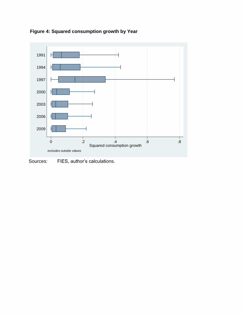
Figure 4: Squared consumption growth by Year

0 .2 .4 .6 .8Squared consumption growth

2009

2006

2003

2000

1997

1994

1991

excludes outside values


Have Filipino Households Become Less Prudent? Akiko · PDF fileHave Filipino Households Become...

Documents

Transcript of Have Filipino Households Become Less Prudent? Akiko · PDF fileHave Filipino Households Become...