CHARLES L. SCHULTZE

Brookings Institution

Has the Phillhs Curve

Shifted? Some Additional

Evidence

IN AN EARLIER ISSUE OF Brookings Papers on Economic Activity, George Perry argued that the Phillips curve, measured in the conventional way, had shifted to the right in recent years, and estimated that a 4 percent over- all unemployment rate would produce about 1 /2 percentage points more inflation per year than was the case in the mid-1950s.1 Perry's conclusion was based on a wage equation that used, instead of the overall unemploy- ment rate, two other measures of labor market conditions: (1) a weighted unemployment rate, in which the unemployment rate for each age-sex group is weighted by the relative hours of work and wage levels of that group; and (2) an unemployment dispersion index, which measures the variance of unemployment rates among different age-sex groups.

The use of weighted unemployment in the wage equation appears to be required simply to take account of the arithmetic of aggregation: A given percentage increase in wages of low-paid and part-time workers has less impact on an aggregate wage index than does the same increase won by higher-paid full-time workers. Perry's use of the dispersion index reflected two hypotheses that appear to be reasonable on a priori grounds: Substitu- tion among different age-sex groups in the labor market is imperfect; and the elasticity of wage response to unemployment increases as the unem- ployment rate decreases. As a consequence, the overall rate of wage in-

1. George L. Perry, "Changing Labor Markets and Inflation" (3:1970), pp. 411-41.

452

Charles L. Schultze 453

crease associated with any given average unemployment rate will be higher the greater the dispersion of group rates about the mean.

The upward shift in the steady-state Phillips curve deduced by Perry stems from two developments: (1) Relative to prime-age male workers, young people and women now make up a higher proportion of the labor force than they did fifteen years ago; because their wages and working hours are typically below the average, the Perry weighted unemployment index has fallen relative to unweighted unemployment. (2) Unemployment rates for young people and teenagers have risen relative to the rate for prime-age male workers; as a consequence, for any given level of unem- ployment, the dispersion of that unemployment is higher than it was in the mid-1950s.

Perry has identified structural reasons for a shift in the Phillips curve. I have tested the existence of such a shift by examining two factors more closely associated with the internal operations of the labor market-the relationships of quits and layoffs to unemployment. Although these rela- tionships tell us nothing about the causal factors, they do suggest that there has indeed been an upward shift in the Phillips curve, by an amount roughly the same as that calculated by Perry.

The relationship between quits and layoffs on the one hand and labor market conditions on the other has been explored by several investigators in recent years.2 But none of them has sought to use the data as a means of testing whether there has been a shift in the Phillips curve.

The Phillips curve can be written as

(1) w (U, Z), where

w = the rate of wage increase U = the overall unemployment rate Z = all other relevant variables.

If the labor force is composed of various groups of workers, distin- guished by differing skills, abilities, experiences, and geographical loca-

2. Sara Behman, "Wage-Determination Process in U.S. Manufacturing," Quarterly Journal of Economics, Vol. 82 (February 1968), pp. 117-42; Charles C. Holt, "Job Search, Phillips' Wage Relation and Union Influence, Theory and Evidence," Working Paper P-69-2 (Urban Institute, March 1969; processed); Charles L. Schultze and Joseph L. Tryon, "Prices and Wages," in James S. Duesenberry and others (eds.), The Brookings Quarterly Econometric Model of the United States (Rand McNally, 1965).

454 Brookings Papers on Economic Activity, 2:1971

tions; if these groups are imperfectly substitutable for each other; and if the relevant wage index excludes the effects of interindustry shifts, then w is aggregated from group wage increases by (2) w- wXRi,

where the subscript denotes labor force groups and R, is a weight whose size depends on both the total number of hours worked and the wage level of the group during some base period.

The Phillips curve, as usually drawn, collapses into one macro-relation- ship what is in reality the aggregation of two micro-relationships. Ex- pressing wage increases as a function of the level of unemployment im- plicitly involves two relationships:

(3) ;Vi gi

and (4) Vi ki(Ui)

Equation (3) states that the rate of wage increase is a function of the excess demand for labor, where excess demand is given by the relationship be- tween the job vacancy rate (V) and the unemployment rate specific to a particular labor force group.

Equation (4) states that the vacancy rate is functionally related to the unemployment rate, as a consequence of which the degree of excess demand in the labor market can be related to the unemployment rate alone. Usually equation (4) is thought to be nonlinear and some variant of the general form (5) VU= a,

since unemployment is inversely related to the vacancy rate and bounded son the lower side by zero.

The gi, in other words, are the behavioral excess demand functions, while the ki are functions that permit use of a surrogate variable U in place of true measures of excess demand.

The aggregate wage equation is: (6) 1-E gi [ki(U,)]Ri.

An aggregate wage rate equation written in terms of an overall unweighted unemployment rate will be stable over time only if the following conditions are met:

Charles L. Schultze 455

1. Weighted unemployment either does not diverge significantly from unweighted unemployment or does so in a systematic cyclical fashion that is picked up by the unweighted unemployment rate. Specifically, a one-time shift in the composition of unemployment toward groups with charac- teristically low pay or low hours of work will cause an upward shift in the Phillips curve, as conventionally drawn, and vice versa.

2. If either the ki or gi are generally nonlinear, an increased dispersion of group unemployment rates about the mean will cause a shift in the Phillips curve.3 There is evidence that the ki are nonlinear, such that the increase in labor market "tightness" associated with a decrease in unemployment is greater at low levels of unemployment than at high levels. Whether the gi are similarly nonlinear is not known. Under these circumstances, any shift in the dispersion of unemployment (not itself related to the level of unem- ployment) gives rise to an upward shift in the Phillips curve. It makes no difference which groups have been responsible for the increase in disper- sion.

3. If the various gi and the various ki are significantly different from one another, a shift in the composition of unemployment (again, not system- atically related to the level of unemployment) can cause a shift in the aggre- gate Phillips curve. A change in composition that also involves a change in the dispersion index would lead to a shift in the Phillips curve, but in this case the direction of the shift would depend upon the specific labor force groups involved in the compositional shift.

4. Finally, if the ki or gi functions themselves shift, the reduced form Phillips curve can shift. Since the ki, which express the relationship of vacancies to unemployment, are themselves reduced forms reflecting a complex set of labor market characteristics and economic conditions, any number of factors could cause them to shift. Changes in technology or in- dustrial hiring practices that increase the substitutability among different labor force groups, for example, would tend to reduce the vacancies as- sociated with low levels of unemployment for any given group.

This paper explores the use of the quit rate and the layoff rate in manu- facturing as alternatives to the unemployment rate as a measure of labor market tightness. It starts with the hypothesis that quits and layoffs pick up many of the factors that affect labor market tightness but are not reflected in the aggregate unemployment rate.

3. If the ki and gi are nonlinear in offsetting ways, this proposition does not hold. But offsetting nonlinearity would produce a linear Phillips curve, which is not observed.

456 Brookings Papers on Economic Activity, 2:1971

Unemployment and the Quit Rate

The monthly data on voluntary quits include all separations initiated by employees. They exclude separation due to deaths, disability, retirement, or entry into the armed forces. While voluntary quits are influenced by many factors, the availability of alternative job opportunities is a major element. In some cases workers find new jobs before they quit their old ones. In other cases they go through a spell of unemployment while seeking better jobs. In April 1969 some 16 percent of the unemployed had volun- tarily quit their prior jobs seeking job advancement. In either case the tightness of the labor market influences the quit rate. The greater the excess demand for labor, the more likely is one employer to hire away workers from another. Similarly a worker's decision to quit his present job in search of a better one is presumably influenced by his own evaluation both of vacancies available and the number of other workers competing for them. In short, the quit rate should be strongly influenced by the relationship between vacancies and unemployment. If, for any of the reasons discussed above (an increase in unemployment dispersion, a shift in the composition of unemployment, a shift in the ki functions), the relationship of aggregate vacancies to aggregate unemployment changes, this should be evident from the quit rate-that is, the quit rate should rise relative to the unemployment rate. The quit rate, therefore, should be a better measure of labor market tightness than the unemployment rate and a change in the quit rate relative to the unemployment rate can be interpreted as a shift in the Phillips curve.

Quit rates are collected by the Bureau of Labor Statistics as part of the establishment survey of employment and earnings. But outside of manu- facturing, the data are available only for the coal, metal mining, and tele- phone industries. Insofar as workers with manufacturing experience are substitutable for workers with other experience in nonmanufacturing in- dustries, the quit rate in manufacturing should be influenced by labor market conditions in a range of industries much wider than manufacturing itself. Nevertheless, the use of the manufacturing quit rate to measure general labor market conditions undoubtedly introduces some error into the results.

Between 1952 and 1965 the relationship between the quit rate and the unemployment rate was close and regular (see Figure 1). But in the five subsequent years the quit rate rose sharply relative to unemployment. The shift in this relationship, as shown in Figure 1 and Table 1, was quite

Charles L. Schultze 457

Figure 1. Relationship of Quit Rate in Manufacturing to Aggregate Unemployment Rate, 1952-71

Annual quit rate (percent)

40

35

@1969

\ 1966 30 - 1968

? 1967

25 -@1970

*\ * /1952-65 relationship

20 - 1971P

0~~~~

15 -

10 _ _

10

0 3 4 5 6 7 8

Unemployment rate (percenzt)

Source: Basic data are from Employment and Earnings, Vol. 17 (May 1971) and various preceding issues. The unidentified plots are for 1952-65. The circled plots are not included in the curve.

a. January-May.

458 Brookings Papers on Economic Activity, 2:1971

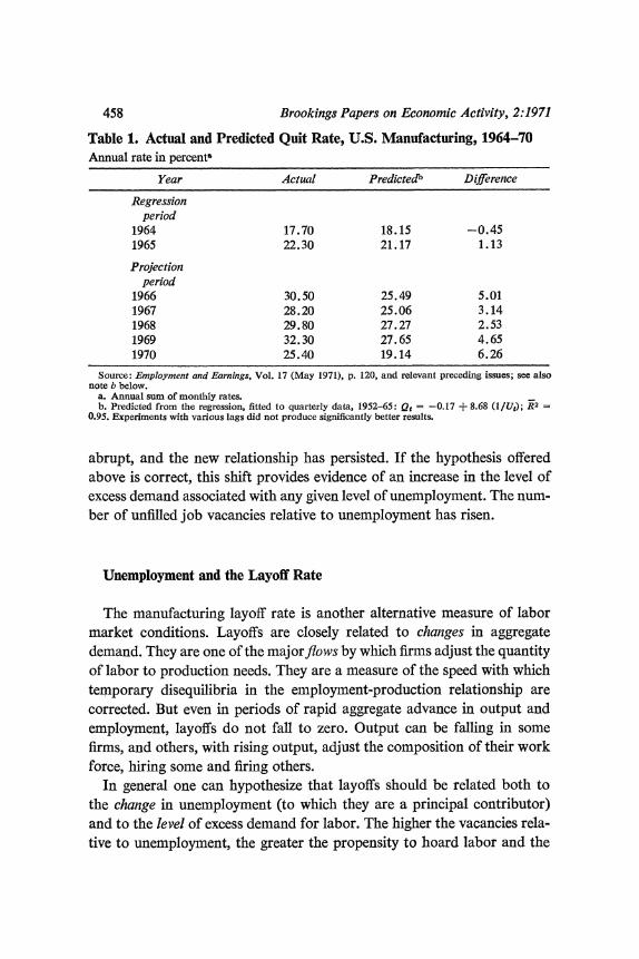
Table 1. Actual and Predicted Quit Rate, U.S. Manufacturing, 1964-70 Annual rate in percent%

Year Actual Predictedb Difference

Regression period

1964 17.70 18.15 -0.45 1965 22.30 21.17 1.13

Projection period

1966 30.50 25.49 5.01 1967 28.20 25.06 3.14 1968 29.80 27.27 2.53 1969 32.30 27.65 4.65 1970 25.40 19.14 6.26

Source: Employment and Earnings, Vol. 17 (May 1971), p. 120, and relevant preceding issues; see also note b below.

a. Annual sum of monthly rates. b. Predicted from the regression, fitted to quarterly data, 1952-65: Qg = -0.17 + 8.68 (1/U,); R2

0.95. Experiments with various lags did not produce significantly better results.

abrupt, and the new relationship has persisted. If the hypothesis offered above is correct, this shift provides evidence of an increase in the level of excess demand associated with any given level of unemployment. The num- ber of unfilled job vacancies relative to unemployment has risen.

Unemployment and the Layoff Rate

The manufacturing layoff rate is another alternative measure of labor market conditions. Layoffs are closely related to changes in aggregate demand. They are one of the majorflows by which firms adjust the quantity of labor to production needs. They are a measure of the speed with which temporary disequilibria in the employment-production relationship are corrected. But even in periods of rapid aggregate advance in output and employment, layoffs do not fall to zero. Output can be falling in some firms, and others, with rising output, adjust the composition of their work force, hiring some and firing others.

In general one can hypothesize that layoffs should be related both to the change in unemployment (to which they are a principal contributor) and to the level of excess demand for labor. The higher the vacancies rela- tive to unemployment, the greater the propensity to hoard labor and the

Charles L. Schultze 459

lower the likelihood of filling jobs made vacant by layoffs. To the extent that unemployment is a surrogate for the excess demand for labor, then, the layoff rate should be explainable by an equation that includes both the level and the change in the unemployment rate. If the vacancy rate associ- ated with any given unemployment rate increases-that is, if labor market conditions are tighter than is implied by the unemployment rate alone- then the layoff rate actually occurring should be less than that predicted by the equation described above.

Table 2 shows the residuals generated by the equation:

Lt = 0.502 + 0.290 U, + 0.354 (U,?1 -U,-), (5.0) (14.8) (13.3)

fZ2 = O.90,DW= 1.97, fit to quarterly data, 1952-62.

The numbers in parentheses are t-ratios.

where L is the monthly manufacturing layoff rate and U is the overall un- employment rate (unweighted). From 1963 on, actual layoffs were sig- nificantly and continually lower than those predicted by the earlier rela- tionship with unemployment. Both the Perry dispersion index and the layoff rate shifted in relationship to unemployment beginning in the early 1960s. The quit rate shift, however, appeared somewhat later, starting in 1966.

Table 2. Actual and Predicted Layoff Rate, U.S. Manufacturing, 1961-70 Annual rate in percent"

Year Actual Predicted Difference

Regression period 1961 27.0 28.0 -1.0 1962 23.5 24.8 -1.3

Projection period 1963 21.8 25.4 -3.6 1964 19.9 22.7 -2.8 1965 17.1 19.7 -2.6 1966 14.4 18.6 -4.2 1967 16.4 19.6 -3.2 1968 14.6 17.5 -2.9 1969 14.2 19.3 -5.1 1970 22.1 27.7 -5.6

Source: Employment and Earnings, Vol. 17 (May 1971), and various preceding issues. a. Annual sum of monthly rates.

460 Brookings Papers on Economic Activity, 2:1971

The Quit and Layoff Rates in Wage Equations

If the quit and layoff rates provide a good measure of the relationship between vacancies and unemployment, they should perform better than unemployment in an equation explaining wage changes. The evidence for this superiority is mixed, but on balance tends to confirm the hypothesis.

In Table 3 eight wage equations are fitted to quarterly data for 1953 to 1968. The eight equations fall into two groups. The first group comprises four alternative versions of Perry's equation (2);4 the alternatives involve four different measures of labor market conditions: the inverse of the un- employment rate, the inverse of Perry's weighted unemployment rate, the manufacturing quit rate, and the inverse of the manufacturing layoff rate.5 The second group is generated by substituting the same four measures of labor market conditions into Perry's equation (3). This latter set of equa- tions includes the two additional measures of labor market conditions dis- cussed by Perry, an index of unemployment dispersion and a measure of secondary employment.6

On the basis of goodness of fit over the 1953-68 period, the quit rate offers no advantage over either the raw or the weighted unemployment rate. Equally clear is the fact that the addition of Perry's supplementary measures of labor market tightness-unemployment dispersion and sec- ondary unemployment-does moderately improve the closeness of fit.

On two other tests, however, the quit rate performs well relative to other measures of labor market tightness. Table 4 shows the lagged one-year cost-of-living coefficients in each of the six equations for three different periods of fit: 1953-64; 1953-68; and 1953-70. Only in the case of equation (ic), the quit rate equation without the other labor market measures, is the cost-of-living coefficient reasonably stable regardless of the period of fit. . The four-quarter wage rate changes, with a three-quarter overlap, are highly serially correlated. If, in turn, wage rate changes are relatively quickly translated into price changes, the cost-of-living variable itself serves as an autocorrelation correction. In equation set 1, when unemploy-

4. Perry, "Changing Labor Markets," p. 425. 5. Since the quit rate is itself related to the inverse of the unemployment rate, it must

be used in its raw form, rather than in its inverse form, in the wage equation. 6. See Perry, "Changing Labor Markets," pp. 412-20, for a description and discussion

of the various measures of labor market conditions. The measure of wage changes used here is also Perry's.

w o o o ~~~~~n o t- llo tn 00

o )

1* Fo F W F CS CF . CS e

a 8 @ 8>^is 8>8@8~~~~~~~~~~~~~~~~~~~~~~~8- ~~~'m tm

z | I o o o o o o o o 1 'm t ?~~~~~~~~~-1

?l 1~~~~~~0 cd

i~~~~~~~~~~~~~~~~~~~~~~~~~~~~~~~~~t X ?? ZU

i~~~~~~~~~~~~~~~~~~~~~~~~0 I % O e R8n C"s IB;

.li i B 2 *- csa *-, @ N @ t- v~~~~~ g v~ v. ? ? ??.8, 6 9 c B.

o~~~~~~~~~~~~~~~% s:o0t 0O5-

is| iz |, en en en en g~ 60 Ci .t en en en cED

o ^ I u I ~~~~~~~e P o oo oo ? lIr n

4B QJ I I Il ^,OXiP

b * SSs'=Xt~C . a X @ > > 9 > > 9 u |> E~~~~~~~ n Q .o g < m m *e Y ? j~~~~~~~~~~~~~~~~~~~~~~~~~~~~~~~~~~~~~~~~~~~~~~~~;

a 44 g _ _ _ a R R N X q X G O a~~~~~~~~~~~~~~~t.

462 Brookings Papers on Economic Activity, 2:1971

Table 4. Lagged Cost-of-living Coefficient in Eight Equations and Three Periods of Fit, 1953-70

Period of fit

Equation number and labor market variable 1953-64 1953-68 1953-70

(la) Inverse of unemployment rate (1/U) 0.374 0.451 0.483 (lb) Inverse of weighted unemployment rate (1/U*) 0.375 0.411 0.443 (1c) Manufacturing quit rate (Q) 0.423 0.435 0.410 (Id) Inverse of manufacturing layoff rate (1/L) 0.569 0.527 0.492 (2a) Inverse of unemployment rate (1/U) 0.372 0.365 0.340 (2b) Inverse of weighted unemployment rate (1/U*) 0.375 0.352 0.332 (2c) Manufacturing quit rate (Q) 0.402 0.357 0.311 (2d) Inverse of manufacturing layoff rate (1iL) 0.462 0.385 0.331

Source: Same as Table 3.

ment (weighted or unweighted) is used as a measure of labor market con- ditions, the cost-of-living coefficients grow substantially larger as recent inflationary years are added to the observations. This is consistent with the hypothesis offered here, namely, that labor markets in the past five or six years are significantly tighter relative to the level of unemployment than they were in the earlier postwar period. The price coefficient, acting as a surrogate for lagged wage increases, would pick up the "excess" wage increases relative to unemployment.

The instability of the price coefficient is most noticeable in the case of the raw unemployment rate. Weighted unemployment in recent years has fallen moderately relative to raw unemployment and its underrepresentation of labor market tightness is slightly less severe. As a consequence the price coefficient, in periods of fit including recent years, has less "correction" to pick up. In the case of the quit rate, the fact that periods of recent fit do not raise the price coefficient is consistent with the hypothesis that quits are a reasonable measure of labor market tightness.

In equation set 2, just the opposite phenomenon occurs. The more recent the period of fit, the lower the price coefficient; and the problem is most severe when quits and layoffs are used as measures of labor market tight- ness and least severe when raw unemployment is used. The Perry dispersion index had a fairly regular relationship to the raw unemployment rate in the years 1952-60 (aside from the anomalous 1953). But starting in 1961, un- employment dispersion rose sharply relative to the unemployment level. To some extent the dispersion index picks up the same increase in labor market tightness as the quit and layoff rates do. As a consequence the two together tend to overpredict wage increases, and in periods of fit that in-

Charles L. Schultze 463

clude recent years, the negative autocorrelation properties of the price variable, when added to its structural properties, produces a decreased coefficient.

The layoff rate, measured in terms of goodness of fit, performs better than any other single measure of labor market tightness (equation ld, Table 4), and about as well as Perry's equation using weighted unemploy- ment and unemployment dispersion. However, the wage equations using the layoff rate exhibit a much higher coefficient on lagged cost-of-living changes than does any of the other equations and less stability in the cost- of-living coefficient than does the quit rate equation.

The point of the preceding analysis is not to demonstrate that the quit rate or the layoff rate is a better measure of labor market conditions than the collection of variables used by Perry. It does, however, lend some sup- port to the a priori reasoning that suggests that the quit and layoff rates are influenced by both vacancies and unemployment, and offers some basis for using the relationship between quits and layoffs to determine whether there has been a shift in the Phillips curve. In particular the evidence sug- gests that the use of quits and layoffs from manufacturing alone to explain general labor market conditions does not introduce so much noise as to invalidate the results.

One other piece of evidence bearing on the suitability of using the manu- facturing quit rate is shown in Table 5, which compares actual wage in- creases with those predicted by the six equations introduced earlier. By the end of the projection period, in late 1970, the equations using unemploy- ment plus Perry's supplementary labor market measures (equations 2a and 2b) are tracking the actual data quite well. So is the equation that uses quit rates alone as a labor market measure (equation ic). The equations using only unemployment are significantly underpredicting while that using both quits and Perry's supplementary measures (equation 2c) is overpredicting. From late 1968 through early 1970, both the equations with Perry's sup- plementary measures (2a and 2b) and the quit rate equation (ic) overpre- dict wage rate increases, but the last does so by a substantially smaller margin. Again there is nothing conclusive about this analysis, but the quit rate still holds up well in comparison with other measures.

The Shift in the Phillips Curve

Figure 2 depicts the steady-state Phillips curve that results from combin- ing the quit rate wage equation (1c) with the quit rate-unemployment

464 Brookings Papers on Economic Activity, 2:1971

Table 5. Predictions of Wage Changes in U.S. Manufacturing, Six Equations, 1967-70 Percent change from prior year

Predicted Equation number and labor market variable

Based on Based on

Year Perry's equation (2) Perry's equation (3)

and (la) (lb) (1c) (2a) (2b) (2c) quarter Actual 1/U 1/U* Q 1/U 1/U* Q

Regression period

1967 1 6.7 6.4 6.5 6.9 6.7 6.8 7.0 2 6.4 6.2 6.3 6.6 6.6 6.6 6.8 3 6.5 6.0 6.2 6.4 6.7 6.7 6.8 4 6.0 (6.9)s 6.1 6.2 6.4 6.9 6.9 7.0

1968 1 7.3 6.1 6.4 6.4 7.1 7.1 7.2 2 7.3 6.6 6.9 6.8 7.6 7.6 7.7 3 7.5 6.9 7.2 7.2 8.0 8.0 8.0 4 8.2 (7.4)a 7.2 7.5 7.3 8.1 8.2 8.1

Projection period

1969 1 7.2 7.6 7.9 7.7 8.5 8.6 8.6 2 7.3 7.7 7.9 8.0 8.7 8.7 8.8 3 7.5 7.9 8.1 8.3 8.8 8.8 9.0 4 7.4 7.9 8.1 8.3 8.9 8.9 9.1

1970 1 7.3 7.6 7.6 8.0 8.4 8.4 8.7 2 7.6 7.3 7.3 8.0 8.2 8.2 8.6 3 8.0 7.0 7.0 7.7 7.9 7.8 8.3

Sources: See Table 3. The residuals were calculated from coefficients estimated in autoregressively corrected regressions, but the autoregressive correction coefficient was not used in making the predictions in order to demonstrate the structural properties of the equations.

a. Actual wage increase data for the fourth quarter of both 1967 and 1968 are aberrant, the former year forming a deep trough between surrounding quarters and the latter year a sharp peak. If the wage increase in 1967:4 is changed to the mean of the increase for the surrounding quarters (on the assumption that the 1967:4 wage level was underreported), the resultant correction for the 1968:4 increase also brings it into line with the surrounding quarters. The "corrected" data are shown in parentheses.

function fitted to 1952-65 data (see footnote b to Table 1). For compari- son with Perry's results, this Phillips curve can also be thought of as apply- ing to the mid-1950s (1956 and 1957); the small positive residuals generated by the wage equation for those years are offset by small negative residuals from the quit-unemployment equation. The two higher tradeoff curves shown in Figure 2 stem from two alternative assumptions about the magni- tude of the upward shift in the quit-unemployment relationship. One alternative uses the difference between actual quits in 1966-70 and those

Charles L. Schultze 465

Figure 2. Shift in the Phillips Curve, Based on Evidence from the Quit Rate in Manufacturing, Selected Periods, Mid-1950s to 1970

Annual price increase (percent)

7

6

5

Tradeoff based on 969-70 quit rates

3

Mid-1950s tradeoff \ .,

2 _ \ Tradeof based N

on 1966-70 quit rates

_ 1\

O AsI I I .I 0 3 4 5 6 7

Untemployment rate (percent)

Source: Based on equation (Ic), Table 3.

466 Brookings Papers on Economic Activity, 2:1971

predicted from the 1952-65 quit-unemployment equation. The second uses the difference between actual and predicted quits only for 1969 and 1970. When the relationships between the quit and unemployment rates are trans- lated into steady-state Phillips curves, via equation (lc) and a 2.7 percent productivity assumption, they suggest that a 4 percent rate of unemploy- ment, if maintained, would generate between 1.2 and 1.5 percent greater price increases than was the case in the mid-1950s.

When the Phillips curve is calculated on the basis of equations using the inverse of layoffs as a measure of labor market pressure, the shift in the curve is somewhat larger. At 4 percent unemployment, the steady-state rate of inflation is 2 to 21/2 percentage points higher, on the basis of recent layoff-unemployment relationships, than was the case in the mid-1950s. The layoff equation generates a larger shift in the Phillips curve than does the quit equation in part because the price coefficient is significantly larger in the layoff equation, and leads to a larger feedback effect.

Summary

Three different measures of labor market conditions-the quit rate, the layoff rate, and the Perry dispersion index-all point toward a significant increase in the labor market tightness associated with any given level of unemployment. In turn, this has been interpreted in terms of an upward shift in the aggregate vacancy-unemployment relationship, and therefore in the curve representing the excess demand for labor.

The behavior of the quit rate and layoff rate themselves tells nothing about the structural changes that have caused the worsening tradeoff between unemployment and inflation. The increase in the Perry dispersion index, on the other hand, does say something about the nature of the problem.

The sharp increase in the proportion of unemployment accounted for by teenagers, young adults, and females, and the corresponding decrease among prime-age males, may affect the aggregate vacancy-unemployment relationship because of the nonlinearity of the ki functions. Or it may rep- resent a compositional shift among groups with different ki functions (for example, the vacancy rate per unit of unemployment for prime-age males is higher than that for teenagers). In this case the problem is not so much dispersion per se as it is the particular compositional shift that underlies

Charles L. Schultze 467

the increase in dispersion. In either interpretation of Perry's results, the problem of increased labor market tightness associated with a 4 percent unemployment rate stems from the very low level to which unemployment among prime-age experienced male workers must be pushed in order for the overall average to reach 4 percent.

Discussion

CHARLES HOLT found Schultze's analysis and results both relevant and significant. However, he wished to question the connection between Schultze's analysis and his policy implications. The moral of the story may be that manpower policies should focus on the groups with very low unem- ployment rates and try to develop programs that would alleviate skill shortages by expanding the flow of available labor to these areas. Such a strategy would be intended to aid the high unemployment groups by re- ducing inflation and making it possible to increase demand and the num- ber of jobs. This strategy might reduce unemployment more successfully than one that focused more directly on groups with excess supply and high unemployment as Schultze suggested.

R. A. Gordon pointed out that, since the data on the quit rate apply only to manufacturing, they may underrepresent teenagers and women, the demographic groups of the labor force that have been increasing most rapidly. Compared with prime-age males, teenagers and women must have relatively high quit rates because they move in and out of the labor force. James Duesenberry noted that scattered data on quits are collected for some nonmanufacturing sectors and suggested that they should be assem- bled and studied. He also regarded the quit rate as important, not merely as a proxy for vacancies or a general labor market indicator, but as a direct object of concern to employers. Firms do not want to lose employees who have acquired some experience and skill, and they will spend money to meet wage competition in order to hold down quits.