1

Harming Depositors and Helping Borrowers:

The Disparate Impact of Bank Consolidation

by

Kwangwoo Park

Graduate School of Finance Korea Advanced Institute of Science and Technology

Seoul 130-722 Republic of Korea

Phone: (822) 958-3540

Email: kpark3@kaist.ac.kr

and

George Pennacchi*

Department of Finance

College of Business University of Illinois

1206 South Sixth Street Champaign, IL 61820

Phone: (217) 244-0952

Email: gpennacc@uiuc.edu

*Corresponding author. We are grateful to the Office for Banking Research at the University of Illinois and the Federal Reserve Bank of Cleveland for research support. Dong Keun Choi and Jaehoon Lee provided excellent research assistance. Valuable comments were provided by Allen Berger, Mark Carey, Nicola Cetorelli, Astrid Dick, Joong Ho Han, Timothy Hannan, Robert Hauswald, Myron Kwast, Sangwoo Lee, Toby Moskowitz (the editor), Robin Prager, Bent Vale, two anonymous referees, and participants of the 2003 Competition in Banking Markets Conference at the Katholieke Universiteit Leuven, the 2004 International Industrial Organization Conference, the 2004 Chicago Fed Bank Structure and Competition Conference, and the 2005 American Finance Association Meetings. We also thank participants of seminars at the University of Alberta, the Bank of Korea, Hitotsubashi University, KAIST, the Korea Institute of Finance, Korea University, the Korea Deposit Insurance Corporation, Seoul National University, and Waseda University.

2

Harming Depositors and Helping Borrowers:

The Disparate Impact of Bank Consolidation

Abstract

A model of multimarket spatial competition is developed where small, single-market

banks compete with large, multimarket banks (LMBs) for retail loans and deposits. Consistent

with empirical evidence, LMBs are assumed to set retail interest rates uniformly across markets,

have different operating costs, and have access to wholesale funding. If LMBs have significant

funding advantages that offset potential loan operating cost disadvantages, then market-extension

mergers by LMBs promote loan competition, especially in concentrated markets. However, such

mergers reduce retail deposit competition, especially in less concentrated markets. Prior empirical

research and our own analysis of retail deposit rates support the model’s predictions.

3

Harming Depositors and Helping Borrowers: The Disparate Impact of Bank Consolidation

Banks in the United States have experienced rapid consolidation in recent years. Restructurings

have been driven by advances in information technology and by deregulation of geographic

restrictions on branching and acquisitions. Since the mid-1980s, the number of commercial

banks and savings institutions more than halved from 17,900 in 1984 to 8,681 in 2006, and

during the same period banks’ average asset size (in inflation-adjusted 2006 dollars) more than

tripled from $348 million to $1.366 billion. Much research has analyzed the competitive effects

of this banking consolidation, especially how mergers impact potentially vulnerable customers,

such as small businesses and consumers.

While banks have become fewer in number and larger on average, there has not been a

systematic increase in the concentration of local banking markets. The Herfindahl-Hirschman

Index (HHI) of deposit shares in Metropolitan Statistical Areas (MSAs) has averaged about the

same as before the merger wave.1 While some horizontal mergers (acquisitions involving two

banks in the same market) have occurred, the major impact of consolidation has been to broaden

the geographic scope of bank operations through market-extension mergers (acquisitions

involving two banks in different markets).

As a result of market-extension mergers, large multimarket banks (LMBs) increasingly

compete with smaller community banks in many local markets. While an LMB’s entry via

acquisition may not directly change a local market’s concentration, there is concern that bank-

dependent customers, such as small businesses and consumers, may be affected. LMBs tend to

use more standardized lending and deposit-taking technologies that may produce cost differences

relative to smaller banks and ultimately affect the interest rates faced by retail customers.

The current paper investigates the competitive effects of market-extension mergers that

4

increase the presence of LMBs in local banking markets. It presents a model that accounts for

three differences between LMBs and small banks that prior research has documented. First,

LMBs’ greater size and organizational complexity can give them costs of providing retail loans

and deposits that differ from those of smaller banks. Second, LMBs standardize their services by

setting retail deposit and loan rates that tend to be uniform across local markets. Third, LMBs

have access to wholesale sources of funding while most small banks do not. The model is used to

analyze how these three differences affect retail loan and deposit competition in local markets.

The paper also examines how the model’s predictions square with empirical evidence.

Our model of multimarket, spatial competition assumes that small banks operate in one

local market while LMBs operate in multiple markets. A small bank sets retail loan and deposit

interest rates based on the competitive conditions in its single market while an LMB chooses

retail rates that are uniform across markets and reflect its differential operating and funding costs,

as well as the competitive conditions in its multiple markets. The model’s Bertrand-Nash

equilibrium shows that retail loan and deposit rates set by banks in a particular market depend

not only on the market’s concentration but also the market’s distribution of LMBs and small

banks.

The model’s most important result is that a greater presence of LMBs tends to promote

competition in retail loan markets but also tends to harm competition in retail deposit markets.

Depending on the relative magnitudes of these two effects, profits of small banks in a given

market can rise or fall with greater penetration by LMBs. We document that several empirical

studies are consistent with these implications. Empirical research finds that a greater presence of

LMBs in a local market tends to lower small business loan rates but also tends to lower retail

deposit rates.

5

The plan of the paper is as follows. The next section reviews research on large and small

bank differences regarding retail loans, retail deposits, and wholesale funding. This evidence

justifies the assumptions made by our model presented in Section 2. The model considers large

and small bank behavior in a setting of multimarket, spatial competition and solves for banks’

equilibrium retail loan and deposit rates. Section 3 examines the model’s implications regarding

a greater presence of LMBs and evaluates these predictions in light of prior empirical research.

Section 4 presents new empirical evidence using Bankrate, Inc. survey data on retail

deposit interest rates. It also analyzes how LMBs’ acquisitions of small banks affects Money

Market Deposit Account (MMDA) interest rates based on Call Report and Thrift Financial

Report data. Section 5 contains concluding remarks.

1. Research on Differences in the Operations of Large and Small Banks

To motivate the modeling assumptions made in the next section, we briefly review three findings

of prior research. First, bank size influences the technology used to make retail loans, thereby

affecting operating costs. Second, LMBs tend to set retail loan and deposit interest rates that are

uniform across markets. And, third, LMBs have access to wholesale sources of funding that are

unavailable to smaller banks.

Theories of organization diseconomies, such as Williamson (1967) and Stein (2002),

predict that LMBs may face higher costs of servicing small businesses and consumers. An

LMB’s top management lacks control of branch-level operations because its complex hierarchy

makes monitoring lower-level employees difficult. As a result, LMB managers may establish

explicit decision rules rather than allow employee discretion, so that loan approval and pricing

decisions rely on “hard” information, such as financial statements and credit histories. In contrast,

6

small banks’ simpler organization permits employee decisions based on “soft information,” such

as the borrower’s “character” and local market conditions. Empirical research by Berger, Miller,

Petersen, Rajan, and Stein (2005), Cole, Goldberg, and White (2004), and Haynes, Ou, and

Berney (1999) supports such large and small bank operating differences.

While there may be diseconomies of scale in utilizing soft information, other economies

of scale are likely to exist. As a bank grows to be an LMB, say via a market-extension merger of

smaller banks, it may eliminate some duplicate activities such as personnel and capital assigned

to product marketing.2 Also, geographic expansion can improve loan portfolio diversification,

thereby decreasing the likelihood of incurring costs due to financial distress. Further, greater size

may justify the fixed costs of determining standard criteria for loan approvals and for loan and

deposit rate setting that reduce the marginal costs of these services.3 Thus, relative to smaller

banks, LMBs may not face a net operating cost disadvantage for retail loans and deposits.4

Greater standardization by LMBs appears to extend to the setting of interest rates on

consumer loans and deposits. Radecki (1998) states that many LMBs have centralized their

management and operations along business, rather than geographic, lines. He documents from

Bankrate, Inc. survey data that an LMB tends to quote rates for a given type of retail loan or

deposit that is the same in different cities throughout a state and often throughout a wider area.

Biehl (2002), Heitfield (1999), and Heitfield and Prager (2004) find that small banks set their

rates based on the competitive conditions in their local MSA, but LMBs set uniform rates

reflecting conditions over a larger region. The growth in Internet advertising may reinforce this

uniformity. By quoting uniform rates, rather than local market-specific ones, LMBs avoid

offending consumers that would be offered a relatively unattractive rate due to their location.

Prior research highlights another difference between large and small banks. Bassett and

7

Brady (2002) document that small banks’ liabilities are mostly Federal Deposit Insurance

Corporation (FDIC)-insured retail deposits, while the liabilities of LMBs include large

proportions of uninsured wholesale funds.5 LMBs, but not small banks, have access to wholesale

financing because institutional investors view LMBs to be more transparent, more

geographically diversified, and/or “too big to fail.”6 Thus, small banks may consider the interest

rate paid on retail deposits as their marginal cost of financing loans whereas LMBs’ marginal

funding cost is a wholesale rate, such as LIBOR.7 Indirect evidence that small banks face limited

financing opportunities stems from empirical tests of a “bank-lending channel” of monetary

policy.8 During monetary contractions, small banks, but not large ones, have difficulty funding

loans, a result consistent with small banks facing retail deposit funding constraints.

Given these differences between LMBs and small banks, let us now consider a

multimarket modeling environment where these two types of banks compete.

2. A Theory of Banking Market Size Structure and Competition

To set the stage for analyzing the rate setting behavior of LMBs and small banks, we begin by

analyzing a Salop (1979) circular city model that is similar to Chiappori, Perez-Castrillo, and

Verdier (1995). We first consider a situation where all banks in a particular market are small,

single-market banks and later analyze markets where some banks have multimarket operations.9

2.1 Basic assumptions

A particular banking market has a continuum of two sets of retail customers: depositors and

borrowers. These customers are located uniformly around a circle of unit length. Each depositor

desires a fixed sized deposit while each borrower wants a fixed sized loan. Let D be the total

8

volume of potential deposits in the market, which equals the product of the market’s density of

depositors and the fixed deposit size. Similarly, denote by L the market’s total volume of

potential loans, equal to the density of borrowers times each borrower’s fixed loan size.

Initially, it is assumed that there are n identical banks located equidistantly around this

unit circle, so that the distance between each bank is 1/n.10 These banks have the same

technologies for producing financial services at constant marginal operating costs of cD per unit

of deposits and cL per unit of loans. cD includes deposit marketing expenses and the costs of

sending monthly statements to depositors, while cL reflects similar direct costs, as well as the

costs of screening a borrower’s credit, of monitoring the borrower, and of default losses.

To obtain these services, customers are assumed to incur a cost of traveling to a bank,

where tD (tL) equals a depositor’s (borrower’s) transportation cost per unit deposit (loan).11 We

assume these linear transportation costs do not exceed the gross surplus from consuming each of

the banking services. Thus, a given bank has a comparative advantage in serving customers that

are closest to it and directly competes for customers with only its two neighboring banks.

Let rL,i be the retail loan rate offered by bank i, and let rL,i-1 and rL,i+1 be the rates given by

its two neighboring banks. A borrower located between bank i-1 and bank i and who is a distance

x- ∈[0, 1/n] from bank i is indifferent between obtaining the loan from bank i-1 and bank i if:

, , 11

L i L L i Lr t x r t xn− − −

⎛ ⎞+ = + −⎜ ⎟⎝ ⎠

. (1)

Similarly, a borrower located between bank i and bank i+1 and who is a distance x+ ∈[0, 1/n]

from bank i would be indifferent between obtaining the loan from bank i and bank i+1 if:

, , 11

L i L L i Lr t x r t xn+ + +

⎛ ⎞+ = + −⎜ ⎟⎝ ⎠

. (2)

Therefore, given these loan rates, bank i’s total demand is (x- + x+)L. Using Equations (1) and

9

(2), bank i faces the loan demand curve of:

( ) , 1 , 1,2

L i L iL i

L

r r L Lx x L rt n

− +− +

+⎛ ⎞+ = − +⎜ ⎟

⎝ ⎠. (3)

Similarly, if depositors are a distance of y- or y+ ∈[0, 1/n] are just indifferent to supplying

deposits to bank i, this bank faces a supply curve of deposits given by:

( ) , 1 , 1, 2

D i D iD i

D

r r D Dy y D rt n

− +− +

+⎛ ⎞+ = − +⎜ ⎟

⎝ ⎠. (4)

Let rW be the wholesale borrowing or lending interest rate, such as LIBOR, and let W be

bank i’s net amount invested at this wholesale rate. Consistent with the evidence discussed in

Section 1, we assume that small single-market banks can invest in wholesale instruments, but

cannot borrow at the wholesale rate rW. Therefore, if bank i is small, it faces the constraint:

0W ≥ . (5)

Later, when LMBs are analyzed, we assume that they have access to wholesale borrowing, in

addition to investing, at rate rW, so that the sign of W is unrestricted for them.

All banks are assumed to face a regulatory capital constraint of the form:

( )( ) max ,0E y y D Wρ + −≥ + + −⎡ ⎤⎣ ⎦ , (6)

where E is the amount of equity capital and ρ is the minimum required equity-to-debt ratio (i.e.,

ρ/(1+ρ) is the minimum capital-to-asset ratio). The cost of issuing equity is given by rE, and we

assume rE > rW due to debt having a lower agency cost and/or a tax advantage relative to equity.

Given these assumptions, a bank’s balance sheet equation takes the form:

( ) ( )W x x L y y D E− + − ++ + = + + . (7)

2.2 Equilibrium with single-market operations

10

We now state the profit maximization problem for a small bank in a given market. It is:

( ) ( ) ( ) ( ), ,

, ,, ,Max

LL i D i

W L i D i D Er r WWr x x L r c y y D r c Er− + − ++ + − − + + − , (8)

subject to the constraints (5) and (6) and subject to the balance sheet equality (7).

As shown in the Appendix, there are two alternative cases for how this bank would

optimally structure its balance sheet. First, if it is optimal for the bank to invest in a positive

amount of wholesale funds (W > 0), then its equity capital constraint (6) must be binding (E =

ρ(y- + y+ )D). This implies that the bank’s optimal loan and deposit rates satisfy:

, 1 , 1,

1 12 2 2

L i L i LL i W L

r r tr r cn

− ++⎛ ⎞ ⎛ ⎞= + + +⎜ ⎟⎜ ⎟ ⎝ ⎠⎝ ⎠. (9)

( ), 1 , 1,

1 12 2 2

D i D i DD i W E W D

r r tr r r r cn

ρ− ++⎛ ⎞ ⎛ ⎞= + − − − −⎜ ⎟⎜ ⎟ ⎝ ⎠⎝ ⎠. (10)

And in a symmetric Bertrand-Nash equilibrium where rL,i = rL,i-1 = rL,i+1 in Equation (9), and rD,i

= rD,i-1 = rD,i+1 in Equation (10), we have:

, /L i W L Lr r c t n= + + . (11)

( ), /D i W E W D Dr r r r c t nρ= − − − − . (12)

This equilibrium holds when the market has total loans less than the total of retail deposits plus

required capital; that is, L < (1+ρ)D. Banks’ excess deposits are invested at the wholesale rate rW,

which is lower than the cost of raising equity, rE, and leads banks to conserve capital. In this

situation, the optimal loan and deposit rates are anchored by the wholesale rate.

Second, if it is optimal for the bank to issue excess equity capital (E > ρ(y- + y+)D), then

its investment in wholesale funds must be zero (W = 0) so that constraint (5) binds. For this

second case, a bank’s optimal loan and deposit rates satisfy:

11

, 1 , 1,

1 12 2 2

L i L i LL i E L

r r tr r cn

− ++⎛ ⎞ ⎛ ⎞= + + +⎜ ⎟⎜ ⎟ ⎝ ⎠⎝ ⎠. (13)

, 1 , 1,

1 12 2 2

D i D i DD i E D

r r tr r cn

− ++⎛ ⎞ ⎛ ⎞= + − −⎜ ⎟⎜ ⎟ ⎝ ⎠⎝ ⎠. (14)

And in a symmetric Bertrand-Nash equilibrium where rL,i = rL,i-1 = rL,i+1 in Equation (13), and rD,i

= rD,i-1 = rD,i+1 in Equation (14), we have:

, /L i E L Lr r c t n= + + . (15)

, /D i E D Dr r c t n= − − . (16)

This second equilibrium occurs when the market’s total loans exceed total deposits plus required

equity capital; that is, L > (1+ρ)D. Banks must now use relatively expensive equity capital to

fund the excess loans, so that the cost of equity, rE, becomes the marginal cost of financing in

Equations (15) and (16).12 This case is consistent with Bassett and Brady’s (2002) empirical

evidence that, relative to large banks, small banks tend to hold more equity capital and have a

greater proportion of their assets in the form of loans.

Comparing the size of the equilibrium retail loan rates in (11) and (15), note that rL,i is

lower for the case when small banks hold positive amounts of wholesale funds because rW < rE.

Similarly, the equilibrium deposit rate in (12) where W > 0 is less than that in (16) where W = 0.

Thus, both deposit and loan rates are lower when money market instruments are the marginal use

of funds compared to when equity capital is the marginal source of funds.

Lastly, to gain intuition for the situation faced by an LMB, suppose that this bank sets

possibly different loan and deposit rates for each of the markets in which it operates, so that

profits are maximized on a market-by-market basis. As mentioned earlier, a key difference

between a small bank and an LMB is that the latter has access to borrowing at the wholesale rate.

12

Hence, this bank’s profit maximization problem for a particular market is given by (8) subject to

(6) and (7), but not the wholesale borrowing constraint (5).

As with a small bank, there are two cases for how an LMB’s balance sheet would be

structured. When it has a positive investment in money market instruments, W > 0, the LMB acts

like a small bank: its optimal loan and deposit rates are the same as (9) and (10). However, for

the alternative case of W < 0, at the margin the LMB’s capital constraint binds and it funds loans

with a proportion 1/(1+ρ) of less expensive wholesale liabilities. Its optimal loan rate takes the

form of the small bank loan rate (13) but with rE replaced by (rW + ρrE)/(1+ρ). In addition, since

wholesale liabilities, not equity, are the marginal funding source, its optimal retail deposit rate is

of the form of the small bank deposit rate (14) but with rE replaced by rW.

Hence, an LMB’s retail loan and deposit rates are lower than those of similarly situated

small banks when wholesale liabilities are its marginal cost of financing. Since empirical

evidence supports LMBs’ reliance on wholesale funds, our analysis that follows focuses on this

case. Also consistent with empirical evidence, we assume that total market loan demand is

sufficiently larger than total deposit supply; that is, ( )1L Dρ+ . This condition will ensure that

in equilibrium small banks fund loans with excess shareholders’ equity, even in markets where

they face competition from LMBs.

2.3 Equilibrium with multimarket operations

We now permit some banks to operate in multiple markets. This new structure can be interpreted

as the result of market-extension mergers, which have no effect on individual market

concentrations. Thus, it is assumed that the numbers of banks in particular circular cities are

unchanged, but merged banks now operate in two markets and are larger. Specifically, assume

13

that small banks in two different markets merge to become an LMB, and the merged banks’ cost

structures and methods of setting interest rates change in the ways described in Section 1.

To simplify the presentation, we start by assuming that only one bank in each of two

markets merges to become an LMB. Thus, if k denotes the number of LMBs in each market, our

beginning assumption is k = 1. As will be shown, extending our analysis to the k ≥ 1 case is easy.

Let us assume that local bank i = 1 is merged with a bank operating in a different circular

city that has m ≤ n banks. We refer to the original market with n banks as the less concentrated

market N, and this market’s total loans and deposits are denoted LN and DN, respectively. The

other local market having m banks is referred to as the concentrated market M, and this market’s

total loans and deposits are denoted LM and DM, respectively. Without loss of generality, assume

that the merged bank (LMB) in market M is also bank i = 1.

As discussed earlier, bank 1’s operating and funding costs can differ from its smaller

rivals due to economies or diseconomies of scale. Specifically, let *Lc and *

Dc be this LMB’s

operating costs of making loans and issuing deposits, respectively, while Lc and Dc remain the

operating costs of small banks. Bank 1 also has access to wholesale funding at the rate rW.

However, its retail interest rates in markets N and M now must be uniform, and its uniform rates

will change the equilibrium interest rates set by the other banks in the two markets.

Assuming, for now, that each of the other banks in the two markets are small single-

market banks, we solve for a Nash equilibrium where all banks set profit maximizing loan and

deposit rates taking their neighboring banks’ rates as given. As will be shown, the equilibrium

rates set by the small banks are no longer equal but differ depending on their distance from the

LMB (bank 1).13 However, the equilibrium is symmetric in the sense that two small banks that

are equidistant from the LMB set the same rates. This situation is illustrated in Figure 1 for the

14

case of a market with a total of eight banks.

We first examine the profit maximization problem for the single LMB, then the profit

maximization problems for the smaller banks in both markets, and, finally, the equilibrium rates

consistent with each bank’s optimization. LMB 1 maximizes the joint profit from operating in

both markets, taking as given the rates of its neighboring banks. Let ,2N

Lr and ,N

L nr ( ,2N

Dr and ,N

D nr ) be

the retail loan (deposit) rates of its two neighboring banks in market N, and let ,2M

Lr and ,M

L mr

( ,2M

Dr and ,M

D mr ) be the retail loan (deposit) rates of its neighboring banks in market M. Given the

aforementioned symmetry in rate setting of small banks that are equidistant from LMB 1, then

, ,2N N

L n Lr r= ( , ,2N N

D n Dr r= ) and , ,2M M

L m Lr r= ( , ,2M M

D m Dr r= ). Hence, generalizing Equations (3) and (4), the

total demand for loans faced by LMB 1 is:

( ) ( ) ( )1 ,1 ,2 ,2 ,2 ,1 ,2 ,1, ,N N M M

L N M N ML L L L L L L

L L

L L L LD r r r r r r rt n t m

≡ − + + − + , (17)

and the total supply of deposits by LMB 1 is:

( ) ( ) ( )1 ,1 ,2 ,2 ,1 ,2 ,1 ,2, ,N N M M

D N M N MD D D D D D D

D D

D D D DS r r r r r r rt n t m

≡ − + + − + . (18)

Then, the LMB 1's profit maximization problem is given by:

( )( ) ( )( ),1 ,1

* *1 ,1 ,2 ,2 ,1 1 ,1 ,2 ,2 ,1,

Max , , , ,L D

L N M D N MW L L L L L D D D D D Er r

Wr D r r r r c S r r r r c Er+ − − + − . (19)

Since we assume that ( )1N NL Dρ+ and ( )1M ML Dρ+ , the LMB’s capital constraint binds,

and it funds loans with both retail deposits and wholesale liabilities (W < 0). The first-order

conditions lead to the solutions:

,2 ,2 *,1

1 11 12 2 2 1

N N M M N ML L W EL

L LN M N Mn mL r L r L L r rtr c

L L L Lρρ

⎛ ⎞+ ⎛ ⎞+ ⎛ + ⎞= + + +⎜ ⎟ ⎜ ⎟ ⎜ ⎟⎜ ⎟+ + +⎝ ⎠⎝ ⎠⎝ ⎠

, (20)

15

( ),2 ,2 *,1

1 11 12 2 2

N N M M N MD D D

D W DN M N Mn mD r D r D Dtr r c

D D D D⎛ ⎞+ ⎛ ⎞+

= − + −⎜ ⎟ ⎜ ⎟⎜ ⎟+ +⎝ ⎠⎝ ⎠, (21)

which shows that LMB 1’s loan and deposit rates depend on market volume – weighted averages

of the rates of its neighboring banks and the concentrations of banks in both local markets.

Turning next to the profit maximization problems of the small banks in each market, note

that they face the same market environment as the LMB in that the volume of loans in each

market exceeds the available retail deposits plus required capital. Thus, small banks, at the

margin, fund loans with equity capital. The small banks in both market N and M choose loan and

deposit rates using the conditions in Equations (13) and (14). However, unlike the basic analysis

of Section 2.1, rL,i-1 ≠ rL,i ≠ rL,i+1 and rD,i-1 ≠ rD,i ≠ rD,i+1 since these banks' loan and deposit rates

differ depending on their distances from LMB 1. The Appendix shows that if ( )1N NL Dρ+

then the loan and deposit rates of the small banks in market N can be written as:

( ), , / , / ,11 , 2,..., / ,N LL i i n k E L i n k L

tr r c r i n kn

δ δ⎛ ⎞= − + + + =⎜ ⎟⎝ ⎠

(22)

( ), , / , / ,11 , 2,..., / ,N DD i i n k E D i n k D

tr r c r i n kn

δ δ⎛ ⎞= − − − + =⎜ ⎟⎝ ⎠

(23)

where recall that k = 1 and for the case that n is an even number:14

( ) ( )( ) ( )

1 12 2

, /2 2

2 3 2 3

2 3 2 3

n ni ik k

i n k n nk k

δ

+ − + −+ + −

≡+ + −

. (24)

Small banks’ rates in market M are identical to Equations (22) to (24) but with n replaced by m.

Equations (22) to (24) show that small bank i’s interest rates are weighted averages of the

16

standard Salop model rates and the rates set by LMB 1, with weights (1-δi,n/k) and δi,n/k,

respectively. The weight δi,n/k on LMB 1’s rates is a declining function of i over the range from i

= 2 to i = n/2 + 1, the mid-point of the circle, and it satisfies the symmetry conditions: δ2,n/k=δn,n/k,

δ3,n/k=δn-1,n/k ,…, δn/2,n/k=δn/2+2,n/k. Thus, as expected, a small bank’s rates are less affected by

LMB 1’s rates the farther is its distance from LMB 1. Moreover, the Appendix shows that for a

given number of bank intervals i, i= 1,…, n away from LMB 1, a small bank’s rates are less

sensitive to the LMB’s rate the greater is the total number of banks in the market; that is,

∂δi,n/k/∂(n/k) < 0. Thus, since n ≥ m, then 0 < δ2,n/k ≤ δ2,m/k < 1, so that rates of small banks in the

more concentrated market M are relatively more sensitive to LMB 1’s rates.

The final step in determining all banks’ equilibrium interest rates is to solve for LMB 1’s

rates given the form of the rates of its neighboring banks in both markets N and M. To find the

LMB’s equilibrium loan rate, we substitute Equation (22) with i = 2 into Equation (20) to obtain:

( )/ /,1

/ / / /

1 1 N MN Mn k m k

L E L L N M N Mn k m k n k m k

n m L LL Lr r c t

L L L Lβ ββ β β β

Λ ++= + + −

+ +, (25)

where ( )/ 2, /2 1n k n kβ δ≡ − > , ( )/ 2, /2 1m k m kβ δ≡ − > , and ( ) ( ) */ 1E W L Lr r c cρΛ ≡ − + + − is the LMB’s

wholesale funding and loan operating cost advantage relative to a small bank. The first three

terms of the right-hand-side of Equation (25) are a weighted average of the equilibrium loan

rates in markets N and M that would exist in the absence of the LMB, where the weights are

βn/kLN /(βn/kLN +βm/kLM) and βm/kLM /(βn/kLN +βm/kLM), respectively. The final term indicates that

when the LMB’s loan rate is lower, the greater is its cost advantage, Λ. Lastly, the equilibrium

retail loan rate of any small bank in either market is found by substituting (25) into (22):

( ), /, /

/ /

1 1i m kM N M NLL i E L n k LN M

n k m k

tr r c L L L tm L L m n

δβ

β β⎡ ⎤⎛ ⎞= + + − Λ + + −⎜ ⎟⎢ ⎥+ ⎝ ⎠⎣ ⎦

. (26)

17

( ), /, /

/ /

1 1i n kN N M MLL i E L m k LN M

n k m k

tr r c L L L tn L L m n

δβ

β β⎡ ⎤⎛ ⎞= + + − Λ + − −⎜ ⎟⎢ ⎥+ ⎝ ⎠⎣ ⎦

. (27)

Since the first three terms on the right-hand-sides of Equations (26) and (27) are the loan rates

that the small banks would set in the absence of the LMB, the presence of an LMB lowers

(raises) small banks’ loan rates if the terms in brackets are positive (negative).

Based on similar logic, the equilibrium deposit rate set by the LMB is derived to be:

( )/ /,1

/ / / /

1 1 N MN Mn k m k

D E D D N M N Mn k m k n k m k

n m D DD Dr r c t

D D D Dβ ββ β β β

Δ ++= − − −

+ +, (28)

where ( )*E W D Dr r c cΔ ≡ − − − is the difference between the LMB’s funding and deposit operating

cost advantages relative to a small bank. Then, the deposit rate of any small bank can be found

by substituting (28) into (23):

( ), /, /

/ /

1 1i m kM N M NDD i E D n k DN M

n k m k

tr r c D D D tm D D m n

δβ

β β⎡ ⎤⎛ ⎞= − − − Δ + − −⎜ ⎟⎢ ⎥+ ⎝ ⎠⎣ ⎦

. (29)

( ), /, /

/ /

1 1i n kN N M MDD i E D m k DN M

n k m k

tr r c D D D tn D D m n

δβ

β β⎡ ⎤⎛ ⎞= − − − Δ + + −⎜ ⎟⎢ ⎥+ ⎝ ⎠⎣ ⎦

. (30)

Thus, an LMB merger lowers (raises) deposit rates if the terms in brackets are positive

(negative).

Having now solved for banks’ equilibrium interest rates when there is k = 1 LMB in each

market, we now discuss why Equations (25) to (30) also hold for an extended model where there

are k ≥ 1 LMBs in each of the two markets. Consider an environment where several market

extension mergers between banks in the two markets result in multiple LMBs symmetrically

located around markets M and N.15 Figure 2 illustrates an example of two LMBs and eight total

banks in market M and 12 total banks in market N. LMBs are at points equidistant around the

two circles, and there are an equivalent number of small banks between each LMB. This

18

symmetry assumption allows us to generalize the previous results because each group of small

banks between any two LMBs faces the same rate-setting problems as those of small banks in a

market with a single LMB. In turn, each LMB is surrounded by an equal numbers of small banks,

making its rate-setting problem analogous to the single merger case.

As in Figure 2 and our earlier analysis, let the number of small banks between each LMB

in markets M and N be odd. The Appendix describes how derivations nearly identical to those of

the single merger case lead to the LMBs and small banks having loan rates equal to Equations

(25), (26), and (27), and deposit rates equal to Equations (28), (29), and (30), but where k ≥ 1.16

3. The Model’s Predictions and Prior Empirical Evidence

Having derived the equilibrium retail loan and deposit rates for LMBs and small banks in

markets of varying concentration, this section analyzes the impact of LMBs on market

competition and whether the model’s predictions are consistent with prior empirical research.

We examine how greater numbers of LMBs affect bank loan rates, deposit rates, and profits.

3.1 The effects of LMBs on loan rates

The effects of LMBs on loan rates in markets N and M depend on Equations (25) to (27).

Analysis of these equations leads to the following proposition.

Proposition 1: Let markets M and N have even numbers of banks equal to m and n, respectively,

and let k of each market’s banks be LMBs located equidistantly around each circle, where 1 ≤ k

≤ m/2 ≤ n/2. If ( ) /1 1N

N M n kLL

m nL Lt β

+Λ>− − , then the loan rates of all small banks in market M are lower

than in the absence of LMBs, and 0Λ> is a sufficient condition for rates to decline as k increases.

19

If ( ) /1 1M

N M m kLL

m nL Lt β

+Λ> − , then the loan rates of all small banks in market N are lower than in the

absence of LMBs, and this is also a sufficient condition for rates to decline as k increases.

Proof: See the Appendix, which also gives exact conditions for loan rates to decline as k

increases.

Proposition 1 says that when LMBs’ loan operating and funding cost advantage, Λ, is

significant, their presence promotes competition in retail loans, particularly in more concentrated

markets. If Λ is close to zero such that ( ) ( )/ /1 1 1 1M N

N M N Mm k n kL LL L

m n m nL L L Lt tβ β

+ +>Λ>−− − , then Equations (25)

to (27) indicate that , ,1 ,N M

L i L L ir r r≤ ≤ . In this case, LMBs mitigate the difference in the markets’

concentrations by setting rates that are intermediate to those of small banks in the two markets

(and intermediate to those that would be set in the absence of LMBs). Loan rates in the more

concentrated market M (less concentrated market N) are lower (higher) than they would be in the

absence of LMBs. Moreover, Λ being non-negative is a sufficient condition for further increases

in the number of LMBs, k, to lower loan rates in the more concentrated market M.

However, if Λ is sufficiently large, an increase in LMBs can reduce loan rates of small

banks in both markets. When ( ) /1 1M

N M m kLL

m nL Lt β

+Λ> − , Equations (25) and (27) indicate that ,1 ,

NL L ir r≤

and increases in k lower small bank loan rates even in the less concentrated market N. Note that

for the special case of m = n where uniform rate setting does not constrain LMBs because both

markets’ concentrations are equal, any Λ > 0 leads to a fall in both markets’ loan rates. This

result would also hold if concentrations were unequal but LMBs set non-uniform, market-

specific rates.

The preponderance of empirical evidence is consistent with LMBs having a funding and

20

operating cost advantage. Studies show that LMBs tend to charge lower retail loan rates

compared to smaller banks and market-wide loan rates tend to be lower when LMBs have a

greater presence. Berger and Udell (1996) examine small business loans using the Federal

Reserve’s Survey of Terms of Bank Lending to Business (STBL) during 1986 to 1994.

Controlling for loan terms and market concentration, they find strong evidence that LMBs charge

lower small business loan rates and require less collateral compared to small banks. Erel (2006)

uses 1987 to 2004 STBL data to study the effects of mergers on small business loan rates,

finding that after a merger, acquiring banks lower their loan rates. She finds that the decline in

rates tends to be especially large when the acquirer is an LMB (has assets exceeding $10 billion).

Berger, Rosen, and Udell (2007) examine lines of credit made to small businesses using

the 1993 Survey of Small Business Finance (SSBF). Controlling for borrower risk and market

concentration, they find that when LMBs have a greater local market share, rates on small

business loans by both LMBs and small banks are lower. They conclude that there is more

aggressive competition for small business credit in markets where LMBs have a greater presence.

3.2 The effects of LMBs on deposit rates

Let us now consider the impact of LMBs on retail deposit rates. Proposition 2 derives from the

LMB and small bank deposit rates given in Equations (28) to (30).

Proposition 2. Let markets M and N have even numbers of banks equal to m and n, respectively,

and let k of each market’s banks be LMBs located equidistantly around each circle, where 1 ≤ k

≤ m/2 < n/2. If ( ) /1 1

m k

MN M Dm nD

D Dt β

+Δ>− − , then the deposit rates of all small banks in market N are

lower than in the absence of LMBs. If ( ) /1 1N

N M n kDD

m nD Dt β

+Δ> − , then the deposit rates of all small

21

banks in market M are lower than in the absence of LMBs, and this is also a sufficient condition

for small banks’ deposit rates in both markets N and M to decline as k increases.

Proof: See the Appendix, which also gives exact conditions for loan rates to decline as k

increases.

Proposition 2 implies that if the difference between an LMB’s funding and deposit

operating cost advantages relative to a small bank, Δ, is significant, then the presence of LMBs

lowers small banks’ retail deposit rates, particularly in less concentrated markets. Note that if Δ

is close to zero such that ( ) ( )/ /1 1 1 1N

N M n k m k

MN MD D

Dm n m nD D

DD D

t tβ β+ +

>Δ>−− − , then Equations (28) to (30)

indicate that , ,1 ,M N

D i D D ir r r≤ ≤ . In this case, LMBs lessen the impact of differences in

concentrations across markets such that all small banks’ deposit rates in the less concentrated

market N (more concentrated market M) are lower (higher) than in the absence of LMBs.

However, if LMBs have a sufficiently large wholesale funding advantage such that

( ) /1 1N

N M n kDD

m nD Dt β

+Δ> − , then an increased presence of LMBs can reduce retail deposit rates even in

the more concentrated market M as well. Moreover, for the special case of m = n, so that the

markets have equal concentrations, deposit rates are lower in both markets whenever Δ is

positive.

Thus, if LMBs have a significant funding advantage as they expand into a market, their

anti-competitive effect on retail deposits is exactly opposite to their pro-competitive effect on

retail loans. Consequently, our model predicts that market-extension mergers may benefit retail

borrowers but harm retail depositors. The intuition for the decline in deposit market competition

stems from an LMB’s unwillingness to compete aggressively for retail deposits if it has a

22

cheaper source of wholesale funding. If, at the margin, an LMB finances loans with wholesale

funds, it would never set a retail deposit rate greater than *W Dr c− , and this constraint is more

likely to bind in less concentrated markets where small banks’ deposit rates would tend to be

higher.

Empirical studies on retail deposit market competition are generally supportive of our

model’s predictions. Empirical work in Hannan and Prager (2004) is motivated by a model

similar to Barros (1999), which assumes that LMBs’ deposit rates are exogenous but uniform

across local markets. It, like our Proposition 2, predicts that the deposit rates paid by small banks

become more like those of LMBs the greater is LMBs’ share of the local market. This

implication is tested using quarterly interest expense and deposit balance data from 1996 and

1999 Call Reports to impute the NOW and MMDA rates paid by small, single-market banks.

They find that these deposit rates diminish as LMBs’ share of the local market rises, primarily

because LMBs’ rates are lower, consistent with a wholesale funding advantage.17

Hannan and Prager (2006a) focus on NOW and MMDA rates paid by multimarket banks

during 2000-2002 and find that rates are lower the larger is the bank’s size.18 They also find that

a multimarket bank’s deposit rate is negatively related to a weighted average of the HHIs of the

markets in which it operates and, even more strongly, to the state-level HHIs where it has a

presence. These findings support the notion that LMBs enjoy a funding advantage and, as in

Equation (28), an LMB’s deposit rate is a deposit-weighted average of the concentrations of its

markets. Hannan (2006) provides related evidence on deposit account fees, which might be

viewed as “negative” deposit interest rates. He finds that LMBs charge higher fees than small

banks and that a greater presence of LMBs raises the fee levels of the local single-market banks.

Our model’s prediction that LMBs compete less aggressively for retail deposits is also

23

consistent with Pilloff and Rhoades (2000) who examine the 1990 to 1996 change in LMBs’

deposit market shares. They find that LMBs retained their market shares in more urban MSAs

but lost them in relatively rural MSAs. Since LMBs obtain wholesale deposits in urban markets

while only retail deposits are obtained in rural markets, these findings are consistent with LMBs’

reliance on wholesale funding and their reluctance to compete for retail deposits.

3.3 The effects of LMBs on bank profitability

This section analyzes how the presence of LMBs affects the overall profitability of banks. To

isolate the effect of an LMB’s wholesale funding advantage from the effect of its uniform rate

setting, consider the case where the concentrations of markets N and M are equal. In this case,

LMBs would charge uniform rates even when permitted to charge different ones. Setting m = n

in the equilibrium loan and deposit rate in Equations (25) to (30) and then calculating banks’

profits based on these rates, it is straightforward to show that the profits of LMBs equal:

( ) ( )2 2

2, / 2, /

/ /

1 11 1n k n kN M N ML D

L n k D n k

L L t D D tn t n t

δ δβ β

⎡ ⎤ ⎡ ⎤− −⎛ ⎞ ⎛ ⎞Λ Δ+ + + + −⎢ ⎥ ⎢ ⎥⎜ ⎟ ⎜ ⎟

⎝ ⎠ ⎝ ⎠⎣ ⎦ ⎣ ⎦, (31)

while the profits of small bank i, i = 2, …, n/k, equal:19

2 2

, / , /

/ /

1 1i n k i n kN NL D

L n k D n k

L t D tn t n t

δ δβ β

⎡ ⎤ ⎡ ⎤⎛ ⎞ ⎛ ⎞Λ Δ− + +⎢ ⎥ ⎢ ⎥⎜ ⎟ ⎜ ⎟

⎝ ⎠ ⎝ ⎠⎣ ⎦ ⎣ ⎦. (32)

The quantities in brackets in (31) and (32) are the individual banks’ equilibrium market shares of

total loans and deposits.20 Thus, a bank’s profit in a loan or a deposit market is proportional to its

squared share of that market. Since 1/n is the average of the n banks’ market shares, when LMBs

have a significant wholesale funding advantage such that Λ and Δ are both positive, LMBs

(small banks) have loan market shares that are greater (smaller) than average. In contrast, LMBs

24

(small banks) have deposit market shares that are smaller (greater) than average.

Moreover, when Λ > 0 the first term in (32) indicates that small banks’ loan market

shares and profits fall as the number of LMBs, k, rises because the factor δi,n/k/βn/k = δi,n/k/(2-δ2,n/k)

rises with k. Furthermore, small banks located closest to an LMB experience the lowest loan

market profits. In contrast, if Δ > 0, the second term in (32) shows that small banks’ deposit

market shares and profits rise with an increase in the number of LMBs, and small banks that are

closest to LMBs have the highest deposit market profits.21 The impact of LMBs on a given small

bank’s total profits can be positive or negative depending on the relative sizes of total market

loans to deposits and differences in loan and deposit transportation and operating costs. Thus, a

greater presence of LMBs may increase small bank profits in some markets but decrease them in

others.

For the general case of m ≤ n, expressions for LMB and small bank profitability are more

complex than (31) and (32). However, note from Propositions 1 and 2 that the competitive

impact of LMBs on loan and deposit markets is relatively greater for the concentrated market M

compared to the less concentrated market N. Hence, all else equal, LMBs are more likely to

reduce small banks’ profits in relatively concentrated markets.22 Intuitively, this is because

LMBs’ uniform rates are averages across markets, so that their loan rates tend to be lower, and

their deposit rates tend to be higher, than those of small banks in concentrated markets.

Since the model predicts that LMBs’ impact on small bank profits are case specific, it is

unsurprising that empirical research on this issue is mixed. Whalen (2001) finds that during

1995-1999 small bank profits were lower when LMBs had greater shares of their MSAs, while

Pilloff (1999b) reports that small bank profits for 1995-1996 in non-MSA rural counties

increased with the presence of LMBs. Using 1985 data for MSAs and rural counties of eight

25

unit-banking states, Wolken and Rose (1991) find that small bank profits declined with LMB

market share.

Berger, Dick, Goldberg, and White (2007) show that a greater LMB market share

increased small bank profitability during the 1980s but decreased it during the 1990s. They

surmise that technological progress in lending allowed LMBs to more effectively compete with

small banks in recent years.23 Finally, Hannan and Prager (2006b) report that during 1996-2003

an increased presence of LMBs reduced small bank profits in non-MSA counties but not in the

less concentrated MSAs. Consistent with our model, they find that impact of LMBs in reducing

small bank profits is the greatest in the most concentrated non-MSA counties.

4. New Evidence on Retail Deposit Competition

This section presents new empirical tests of our model’s predictions regarding retail deposit

market competition. We first examine equilibrium in a static setting using Bankrate, Inc. survey

data. Second, we use Call Report and Thrift Financial Report data to investigate the dynamics of

MMDA rates before and after LMBs’ acquisitions of small banks.

4.1 Evidence using Bankrate survey data

This section analyzes individual LMB and small bank retail deposit rates observed in different

local markets. We begin by describing the data used in our tests.

4.1.1 Data and sample selection. Our data include retail deposit interest rates from annual

Bankrate, Inc. surveys of individual commercial banks and thrift institutions over the seven-year

period from 1998 to 2004. The deposit rates are for MMDAs, six-month maturity retail

26

Certificates of Deposits (CDs), and one-year maturity retail CDs paid by banks in up to 145

different MSAs. The date of each year’s survey is chosen to be the last week of June so as to

match annual FDIC Summary of Deposits (SOD) data. The SOD data record the amount of

deposits issued by individual banks in each MSA and are used to calculate the total deposits

(market size) and the HHI of each MSA, as well as each of our sample bank’s deposits issued

both within and outside of the surveyed MSAs. In addition, as a proxy for an LMB’s wholesale

funding cost, we obtained one-, six-, and twelve-month LIBOR corresponding to the survey

dates from the British Bankers’ Association.

The Bankrate data is attractive because it contains the actual MMDA and retail CD rates

paid by an individual bank at a given date in a particular local market. However, not all MSAs

and not all banks in a given MSA are surveyed by Bankrate. The first column in Table 1 lists the

number of MSAs surveyed in each of the seven years, with 130 MSAs per year being the average.

Bankrate tends to select large- and medium-sized MSAs.24 It surveys ten banks in each of

the largest MSAs, but fewer in the others, with 5.6 being the average. Because Bankrate surveys

relatively large MSAs, and within those MSAs it selects banks with the highest market shares,

large banks are more likely to be surveyed than smaller ones. In our tests, we define an LMB as

any bank having greater than $10 billion in total deposits while a small bank is one with less than

$1 billion in total deposits. Columns three and five in Table 1 gives the total number of small

bank and LMB observations per deposit type and year. In only a handful of cases was a given

small bank surveyed in more than one MSA. However, there were approximately 51 different

LMBs surveyed per year, and, on average, an LMB was surveyed in 9.7 different MSAs.

4.1.2 Deposit rates: small banks versus LMBs. Our model assumes that LMBs set uniform rates

27

across markets and have access to wholesale funding. We now show that the data are consistent

with these assumptions. LMB rates tend to be uniform across the surveyed markets. Also, LMBs

appear to have access to lower-cost wholesale funding because they do not compete aggressively

for retail deposits. Large bank MMDA and retail CD rates tend to be lower than those of small

banks.

In Table 1, columns two and four give the mean MMDA and CD rates offered by small

banks and LMBs for the years 1998 to 2004.25 It also reports in column six a measure of LMB

“rate diversity,” defined as the proportion of markets in which a given LMB is surveyed for

which it sets different rates. Specifically, the statistic reported is the median for all LMBs of:

Number of Different Survey Rates Quoted by an LMB - 1Rate Diversity = Number of Markets in which the LMB Was Surveyed -1

. (33)

Notice that if an LMB sets a uniform rate across all markets, its rate diversity equals 0, while if it

sets different rates in each market, its rate diversity equals 1. Column six of Table 1 shows that

the tendency for LMBs to set uniform rates increased over the sample period. We also found that

if an LMB’s rate diversity is calculated at the state, rather than national, level, the median value

was 0.0 for all deposit types for each of the years, indicating strong state-wide uniformity. This is

consistent with the findings of Radecki (1998).

Table 1 reports that during each of the seven years, and for both MMDAs and CDs, the

average deposit rates offered by small banks exceeded the corresponding average rates offered

by LMBs. Moreover, the mean LMB retail rates were always lower than their equivalent

maturity LIBOR, but this was not always the case for the mean small bank rates.

A simple comparison of mean deposit rates fails to control for possible differences in the

structure of markets in which small banks and LMBs operate. To control for differences, for each

small bank surveyed by Bankrate, we computed the spread between the small bank’s deposit rate

28

and the average of the rates paid by the LMBs in that small bank’s local market. Columns 8-11

of Table 1 show that the average spreads based on this market-by-market calculation are

significantly positive at better than a 99% confidence level for each type of deposit and each year.

These results provide clear evidence that LMBs do not compete for retail deposits as

aggressively as small banks, and they match the empirical research discussed previously.

4.1.3 The effect of LMB market share on retail deposit rates. Recall that Proposition 2 predicts

that LMBs’ uniform rate setting lessens the impact of market concentration on smaller banks’

deposit rates and, if LMBs have a significant funding advantage, their greater presence reduces

small bank deposit rates primarily in less concentrated markets. We test this proposition by

regressing individual banks’ retail deposit rates on market structure and bank size variables. The

dependent variables in these regressions are MMDA, six-month CD, or one-year CD rates. The

explanatory market variables are the MSA’s concentration level (HHI), the natural log of total

MSA deposits as a proxy for market size (Ln (MSADep)), and the share of the MSA’s total

deposits issued by LMBs (LMB Share). Another explanatory variable is a bank size dummy

variable that equals 1 if the bank is an LMB, and zero otherwise (LMB Dummy). Also, as

explained below, an interaction variable, the product of HHI and LMB Share, is included.26

If, as Table 1 suggests, LMBs have a wholesale funding advantage that reduces the rate

they are willing to pay on retail deposits, then the regression’s LMB dummy variable will have a

negative coefficient. The coefficient on HHI also is expected to be negative since, all else equal,

deposit rates are lower in more concentrated markets. Furthermore, Proposition 2 predicts that

the coefficients on LMB Share and LMB Share*HHI should be negative and positive,

respectively. The rationale is that a greater presence of LMBs lowers other banks’ deposit rates

29

in less concentrated markets, but the reduction is less (and may even become an increase) in

more concentrated markets. Hence, LMB Share’s impact on lowering deposit rates should be

greatest when HHI is low but mitigated as HHI rises. Finally, since less concentrated MSAs with

high LMB market shares are often large MSAs, we include the log of total MSA deposits to

reduce the possibility that market size-related factors might bias the other variables’ coefficient

estimates.

Panel A of Table 2 presents results for MMDA interest rates based on cross-sectional

regressions for each year from 1998 to 2004. As expected, the coefficient on HHI is always

negative and is statistically significant for three of the seven years. The coefficient on LMB

Dummy is negative and highly significant in all cases, a result consistent with the evidence in

Table 1. The coefficients on LMB Share and HHI*LMB Share are of the predicted signs

(negative and positive, respectively) for four of the seven years, but they are often not

statistically significant. An indication of the explanatory variables’ effects for the entire sample

period is given in the last column of the table, which reports the time series averages of the year-

by-year regression coefficients along with their Fama-MacBeth standard errors. It shows that

HHI, LMB Dummy, LMB Share, and HHI*LMB Share all have their expected signs and are

statistically significant except for the variable LMB Share.

Panel B of Table 2 repeats the regressions in Panel A but accounts for the fact that some

LMBs do not set perfectly uniform rates and, instead, may vary rates based on local market

conditions. If this were the case, then one would expect LMB Share to have a smaller effect since

LMBs would set rates similar to small local banks. Hence, we replace LMB Share with LMB

Share*(1-RD), where RD is the average of the rate diversities for the LMBs surveyed in the

MSA. The results with this modification are qualitatively similar to those in Panel A; perhaps

30

because RD is relatively small in most markets. In particular, the Fama-MacBeth coefficient for

HHI*LMB Share*(1-RD) remains positive and statistically significant.

Tables 3 and 4 report similar year-by-year regressions for six-month CD rates and one-

year CD rates, respectively. The results in these two tables are similar to each other, and are even

more aligned with the model’s predictions. The coefficient on LMB Dummy is always

significantly negative, and the coefficient on HHI is always negative and is statistically

significant in over 85% of the cases. Also, the coefficients on LMB Share and HHI*LMB Share

[or LMB Share*(1-RD) and HHI*LMB Share*(1-RD)] have their expected negative – positive

signs over 82% of the time and are statistically significant almost 40% of the time. Based on the

Fama-MacBeth coefficient averages, these variables always have their expected signs and are

statistically significant in all but one instance.

Table 5 gives regression results that pool the seven years of data for each deposit type. In

addition to the previously described explanatory variables, these regressions include dummy

variables to account for time fixed-effects. In all cases, coefficients on HHI and LMB Dummy are

significantly negative. In five of six cases, the coefficients on LMB Share or LMB Share*(1-RD)

have their expected negative signs, but are statistically significant only once. However, the

coefficients on HHI*LMB Share or HHI*LMB Share*(1-RD) are always significantly positive.27

As an example of the economic significance of these estimates, consider the six-month

CD regression results in column three of Table 5. They imply that the rates paid by LMBs are

27.3 basis points lower than other banks. They also imply that if the MSA was less concentrated

such that the HHI was lower by 1000, then six-month CD rates would be higher by 17.0 basis

points if there were no LMBs in the market but they would be only 9.65 basis points (0.170 –

0.50*0.147) higher if LMBs had a 50% share of the market.

31

4.2 Evidence from LMB acquisitions of small banks

The previous section’s results are consistent with our theory’s prediction that LMBs pay lower

retail deposit rates and that their greater presence in an MSA tends to reduce deposit rates.

However, there is the possibility that the association between lower deposit rates and a greater

LMB presence has an alternative explanation if our previous tests omitted a variable that affects

both LMB presence and deposit rates. This section attempts to provide additional support for a

causal relationship between LMB market share and lower deposit rates by analyzing the

dynamics of deposit rates around the time of an LMB’s acquisition of a small bank.

Similar to Focarelli and Panetta (2003), we examine the dynamics of deposit rates paid

by banks involved in a merger. A finding that the small bank’s deposit rate prior to a merger is

higher than that of the acquiring LMB after the merger would be consistent with a causal

relationship between LMB presence and lower deposit rates. An alternative finding of no decline

in the pre- and post-merger rates would lend credence to another explanation for the link

between LMB presence and lower deposit rates.

4.2.1 Data and sample selection. We searched annual SOD data on all MSAs for 1994-2005 to

identify instances where a small, single-market bank was acquired by an LMB. Our tests use

both narrow and broad definitions of small banks and LMBs. Small, single-market banks are

defined as having total deposits below $1 billion with at least 75% (narrow definition) or 50%

(broad definition) of their deposits in a single MSA. LMBs are defined as having total deposits

exceeding $10 billion (narrow definition) or $5 billion (broad definition).28 Similar to prior

studies on deposit competition, we calculated implicit MMDA rates for commercial banks using

32

the bank’s quarterly Call Report data on MMDA interest expense and deposit balances. For thrift

institutions, MMDA rates were based on their weighted average cost of MMDAs as reported on

their Thrift Financial Reports. MMDA rates for the acquired small bank and the acquiring LMB

were estimated as of mid-year for the year prior to the acquisition. Also, mid-year MMDA rates

for the LMB were estimated for each of the three years after the acquisition. MMDA rates were

also estimated for each of the other banks in the small bank’s MSA over this four-year period.29

For an acquisition to be included in our analysis, we required that an MMDA rate be

available for the acquired small bank and the acquiring LMB for the year prior to the merger.

Because data needed for calculating MMDA rates are often missing, this requirement led us to

drop many potential merger observations. Under the narrow definitions of small banks and

LMBs, there were 48 acquisitions that met our sample selection criteria. For the broader

definitions, 74 acquisitions met our criteria.

4.2.2 Pre- and post-acquisition MMDA rates. As a benchmark for comparing MMDA rates for

the small bank and the LMB involved in the merger, we calculated the spreads between their

MMDA rates and the average of MMDA rates for the other banks in the small bank’s MSA. We

then compared the acquired small bank’s pre-merger spread to the acquiring LMB’s pre- and

post-merger spreads to see if there were statistically significant differences. The results are given

in Table 6.

Panel A of Table 6 reports tests using the sample of 48 acquisitions meeting the narrow

definitions of small banks and LMBs. The first two rows show that the mean and median

MMDA spreads for the acquiring LMBs were somewhat lower than those of the acquired small

bank in the year prior to the merger, though the difference is not statistically significant. In rows

33

three and four we then examine the 34 of 48 mergers for which MMDA spreads could be

computed one year after the merger. Here we see that for this sample the LMB’s post merger

spread was significantly lower than the small bank’s pre-merger spread. Specifically, the mean

pre-merger small bank spread was + 6.5 basis points while the mean post-merger LMB spread

was -39.1 basis points. Rows five and six show that of the 25 mergers for which MMDA spreads

could be computed two years after the merger, the LMBs’ post merger spread was, again,

significantly lower than their acquired small banks’ pre-merger spread. For three years after the

merger, there is an average pre-merger small bank spread of 15 basis points and a post-merger

average LMB spread of -15 basis points, but the difference is not significant.

Panel B of Table 6 reports results for the broader definitions of small banks and LMBs.

Here, the number of merger observations is larger and the statistical significance of the pre- and

post-merger spread differences is greater. The mean and median spreads of the acquiring LMBs

for one, two, and three years following the merger are always significantly lower than those of

the acquired small bank in the year prior to the merger. The decline in the average spread from

the year before to one, two, and three years after the merger is 37, 48, and 37 basis points,

respectively. In summary, these results are consistent with a causal relationship between LMB

presence and lower deposit rates and present a challenge to alternative explanations.

5. Concluding Remarks

Prior empirical research finds that, relative to small banks, LMBs have more standardized

operations and set retail interest rates that are uniform across many local markets. LMBs also

differ from their smaller rivals in their ability to access wholesale financing. Our model of

multimarket competition accounts for these findings and analyzes competition for retail loans

34

and deposits when LMBs command a greater presence in local markets.

Our model predicts that if LMBs have a significant funding advantage that is not offset

by a loan operating cost disadvantage, their rates on retail loans will be lower than their smaller

bank competitors, especially in more concentrated markets. A greater presence of LMBs

intensifies competition for retail loans and reduces small banks’ loan rates. Interestingly, in such

a situation, LMBs’ effect on retail deposit market competition is the opposite. When LMBs have

a significant wholesale funding advantage, they will not compete aggressively for higher-cost

retail deposits. As a result, their smaller rivals can pay lower rates on retail deposits than

otherwise, especially in less concentrated markets.

Our theory’s predictions are consistent with prior empirical studies, as well as the new

empirical findings presented in this paper. Greater market share by LMBs is associated with

increased competition in small business lending but reduced competition in retail deposit taking.

The impact of LMBs on overall small bank profits depends on the relative magnitudes of these

two opposing effects. Our analysis underscores the likelihood that market-extension mergers,

which increase the scope of LMBs, have disparate welfare consequences for different types of

bank customers.

While our analysis has been in the context of banking, our theory is applicable to other

industries where some competitors operate in multiple markets and set prices uniformly. For

example, our model could be applied to a chain store retailer whose centralized management sets

uniform prices for a wide geographic area that covers multiple local markets of varying

concentrations. Such firms would enhance competition primarily in concentrated markets,

forcing a lowering of prices by single-market retailers. A general effect from the spread of

multimarket competitors is to reduce the variation in prices across local markets.

35

Appendix

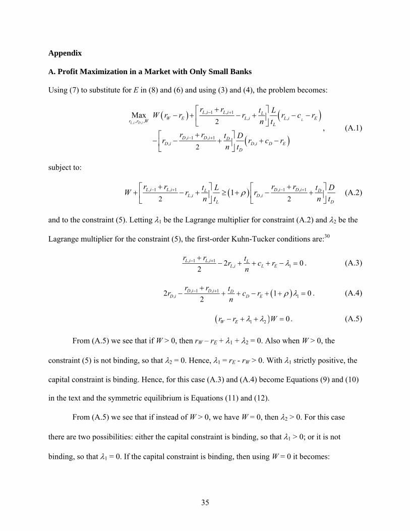
A. Profit Maximization in a Market with Only Small Banks

Using (7) to substitute for E in (8) and (6) and using (3) and (4), the problem becomes:

( ) ( )

( )

, ,

, 1 , 1, ,, ,

, 1 , 1, ,

2

2

Max

LL i D i

L i L i LW E L i L i Er r W

L

D i D i DD i D i D E

D

r r t LW r r r r c rn t

r r t Dr r c rn t

− +

− +

+⎡ ⎤− + − + − −⎢ ⎥

⎣ ⎦+⎡ ⎤

− − + + −⎢ ⎥⎣ ⎦

, (A.1)

subject to:

( ), 1 , 1 , 1 , 1, ,2 2

1L i L i D i D iL DL i D i

L D

r r r rt tL DW r rn t n t

ρ− + − ++ +⎡ ⎤ ⎡ ⎤+ − + ≥ + − +⎢ ⎥ ⎢ ⎥⎣ ⎦ ⎣ ⎦

(A.2)

and to the constraint (5). Letting λ1 be the Lagrange multiplier for constraint (A.2) and λ2 be the

Lagrange multiplier for the constraint (5), the first-order Kuhn-Tucker conditions are:30

, 1 , 1, 12 0

2L i L i L

L i L Er r tr c r

nλ− ++

− + + + − = . (A.3)

( ), 1 , 1, 12 1 0

2D i D i D

D i D Er r tr c r

nρ λ− ++

− + + − + + = . (A.4)

( )1 2 0W Er r Wλ λ− + + = . (A.5)

From (A.5) we see that if W > 0, then rW – rE + λ1 + λ2 = 0. Also when W > 0, the

constraint (5) is not binding, so that λ2 = 0. Hence, λ1 = rE - rW > 0. With λ1 strictly positive, the

capital constraint is binding. Hence, for this case (A.3) and (A.4) become Equations (9) and (10)

in the text and the symmetric equilibrium is Equations (11) and (12).

From (A.5) we see that if instead of W > 0, we have W = 0, then λ2 > 0. For this case

there are two possibilities: either the capital constraint is binding, so that λ1 > 0; or it is not

binding, so that λ1 = 0. If the capital constraint is binding, then using W = 0 it becomes:

36

( ), 1 , 1 , 1 , 1, ,2 2

1 0L i L i D i D iL DL i D i

L D

r r r rt tL Dr rn t n t

ρ− + − ++ +⎡ ⎤ ⎡ ⎤− + − + − + =⎢ ⎥ ⎢ ⎥

⎣ ⎦ ⎣ ⎦, (A.6)

or solving for the deposit rate:

( ), 1 , 1 , 1 , 1

, ,2 21D i D i L i L iD D L

D i L iL

r r r rt Lt tr rn Dt nρ

− + − ++ +⎡ ⎤= − + − +⎢ ⎥+ ⎣ ⎦

. (A.7)

But using the first-order conditions (A.3) and (A.4) and substituting out for λ1 implies:

, 1 , 1 , 1 , 1, ,

1 12 2 4 2

11

D i D i L i L iD LD i D E L i L E

r r r rt tr c r r c rn nρ

− + − ++ +⎡ ⎤ ⎡ ⎤⎛ ⎞= − − + + − − + +⎜ ⎟⎢ ⎥ ⎢ ⎥+ ⎝ ⎠⎣ ⎦ ⎣ ⎦. (A.8)

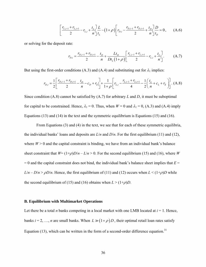
Since condition (A.8) cannot be satisfied by (A.7) for arbitrary L and D, it must be suboptimal

for capital to be constrained. Hence, λ1 = 0. Thus, when W = 0 and λ1 = 0, (A.3) and (A.4) imply

Equations (13) and (14) in the text and the symmetric equilibrium is Equations (15) and (16).

From Equations (3) and (4) in the text, we see that for each of these symmetric equilibria,

the individual banks’ loans and deposits are L/n and D/n. For the first equilibrium (11) and (12),

where W > 0 and the capital constraint is binding, we have from an individual bank’s balance

sheet constraint that W= (1+ρ)D/n – L/n > 0. For the second equilibrium (15) and (16), where W

= 0 and the capital constraint does not bind, the individual bank’s balance sheet implies that E =

L/n – D/n > ρD/n. Hence, the first equilibrium of (11) and (12) occurs when L < (1+ρ)D while

the second equilibrium of (15) and (16) obtains when L > (1+ρ)D.

B. Equilibrium with Multimarket Operations

Let there be a total n banks competing in a local market with one LMB located at i = 1. Hence,

banks i = 2, …, n are small banks. When ( )1L Dρ+ , their optimal retail loan rates satisfy

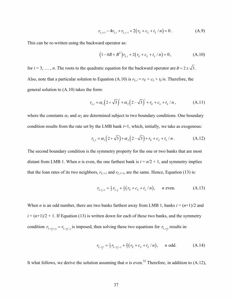
Equation (13), which can be written in the form of a second-order difference equation.31

37

( ), 1 , , 14 2 / 0L i L i L i E L Lr r r r c t n+ −− + + + + = . (A.9)

This can be re-written using the backward operator as:

( ) ( )2,1 4 2 / 0L i E L LB B r r c t n− + + + + = , (A.10)

for i = 3, … , n. The roots to the quadratic equation for the backward operator are 2 3B = ± .

Also, note that a particular solution to Equation (A.10) is rL,i = rE + cL + tL/n. Therefore, the

general solution to (A.10) takes the form:

( ) ( ), 1 22 3 2 3 /i i

L i E L Lr r c t nα α+ −= + + + + , (A.11)

where the constants α1 and α2 are determined subject to two boundary conditions. One boundary

condition results from the rate set by the LMB bank i=1, which, initially, we take as exogenous:

( ) ( ),1 1 22 3 2 3 /L E L Lr r c t nα α+ −= + + + + . (A.12)

The second boundary condition is the symmetry property for the one or two banks that are most

distant from LMB 1. When n is even, the one farthest bank is i = n/2 + 1, and symmetry implies

that the loan rates of its two neighbors, rL i-1 and rL,i+1, are the same. Hence, Equation (13) is:

( )2 2

, ,11 12 2 / , even.n nL L E L Lr r r c t n n+ = + + + (A.13)

When n is an odd number, there are two banks farthest away from LMB 1, banks i = (n+1)/2 and

i = (n+1)/2 + 1. If Equation (13) is written down for each of these two banks, and the symmetry

condition 1 12 2

, ,2 1n nL Lr r+ ++ −= is imposed, then solving these two equations for 1

2, nLr + results in:

( )1 12 2

, , 11 23 3 / , odd.n nL L E L Lr r r c t n n+ + −= + + + (A.14)

It what follows, we derive the solution assuming that n is even.32 Therefore, in addition to (A.12),

38

the second boundary condition is based on (A.13). Substituting (A.11) into (A.13), simplifying,

and noting that ( ) ( ) 12 3 2 3

−− = + , leads to a proportional relationship between α1 and α2:

( ) 2

2 1 2 3n

α α+

+= . (A.15)

Using (A.15) to substitute for α2 in boundary condition (A.12), one finds the solution for α1 to

be:

( )

( ) ( ),1

12 3 1 2 3

/L E L Ln

r r c t nα

+ + +

− + +=

⎡ ⎤⎢ ⎥⎣ ⎦

. (A.16)

Using (A.15) and (A.16) to substitute for α1 and α2 in (A.12), we obtain the solution:

( )( ), , , ,11 / , 1,...,L i i n E L L i n Lr r c t n r i nδ δ= − + + + = , (A.17)

which shows that rL,i is a weighted average of rates with the weight on LMB 1’s rate being:

( ) ( )( ) ( )

1 12 2

,2 2

2 3 2 3

2 3 2 3

n ni i

i n n nδ

+ − + −+ −

+ −

+≡

+. (A.18)

Note that (A.18) satisfies the symmetry conditions: δ2,n=δn,n, δ3,n=δn-1,n ,…, δn/2,n=δn/2+2,n. Its

derivative with respect to i is:

( )( ) ( )

( ) ( )1 1. 2 2

2 2

2 32 3 2 3

2 3 2 3

ln n ni ii n

n niδ + − + −+

− +

+ −

⎡ ⎤∂= −⎢ ⎥∂ ⎣ ⎦+

. (A.19)

Since ( ) ( )0 2 3 1 2 3< − < < + , ∂δi,n/∂i < 0 over the range from i = 2 to i = n/2 + 1, the mid-

39

point of the circle. This implies that a small bank rate’s weight on LMB 1’s rate declines the

further is its distance from LMB 1. The derivative of (A.18) with respect to n is:

( )( ) ( )

( ) ( )2 2

1 1,2

2 3 2 3

2 32 3 2 3

lnn n

i ii n

nδ − −

+ −

+− +

+

∂ ⎡ ⎤= −⎢ ⎥⎣ ⎦∂ ⎡ ⎤⎢ ⎥⎣ ⎦

. (A.20)

Since i =2,…, n for the small banks, ∂δi,n/∂n < 0. This means that the rate charged by a small

bank of a given distance i – 1 from LMB 1 will have a smaller weight on LMB 1’s rate the less

concentrated is the market. In other words, keeping distance constant, LMB 1’s rate has less

impact on a small bank’s rate the greater is the number of small banks in the market.

For the general case of a market with n total banks having k ≥ 1 LMBs located

symmetrically around the circle, let the number of small banks between any two LMBs, (n/k) – 1,

be an odd integer. Then the same derivation as above applies to each (n/k) – 1 group of small

banks bordered by two LMBs.33 A small bank’s rate is given by Equation (A.17) except that δi,n

is replaced with δi,n/k, where δi,n/k is given by Equation (A.18) but with (n/k) replacing n. This is

exactly Equations (22) and (24). Since ∂δi,n/k/∂(n/k) = ∂δi,n/∂n < 0, we have ∂δi,n/k /∂k = - (n/k2)

[∂δi,n/k/∂(n/k)] > 0. This implies that given n, small banks’ rates place greater weight on the rate

of the LMBs the greater is the number of LMBs in the market. Each LMB’s rate setting problem

is the same as in the k = 1 case, such that its equilibrium loan rate equals (25) and, inserting this

back into its neighboring small bank’s loan rate, one obtains Equation (27). The same derivation

is used to find small bank loan rates in market M and deposit rates in markets N and M.

C. Proofs of Propositions 1 and 2

To prove Proposition 1, note from the last terms in Equations (26) and (27) that the presence of

40

LMBs lowers all small banks’ loan rates in markets M and N when:

( ) ( )/1 1N M N

n k L m nL L L tβΛ + > − − and ( ) ( )/1 1N M M

m k L m nL L L tβΛ + > − , respectively. To find the

conditions on Λ for which small bank loan rates in market M decline as k, the number of LMBs,

increases, we differentiate (26) and find that , / 0ML ir k∂ ∂ < when:

( ) ( ), /// /

/1 1

,

,

i m kn k

Nn k m kMn k

L MNi mLm n

N M Li m

Lk LLL t

L L

β ββδβ

∂∂Ψ + +−

Λ > −+ Ψ

, (A.21)

where ( ) ( ), / / /, / / , /

i m k n k m kL N M N Mi m n k m k i m kk k kL L L Lδ β ββ β δ∂ ∂ ∂

∂ ∂ ∂Ψ ≡ + − + >0. In (A.21), since βn/k = (2 -

δ2,n/k) > 0 and ∂βn/k/∂k = - ∂δ2,n/k /∂k < 0, then ( ), // /

/0i m k

Nn k m kMn k

M Lk L

L β ββδ ∂

∂ + < , which permits us to

show that ( ), // /

/, ,1 / 0i m k

Nn k m kMn k

L M Li m i m

Lk LL β β

βδ ∂∂Ψ Ψ⎡ ⎤≥ + + >⎣ ⎦ . Thus, a sufficient condition

for , / 0ML ir k∂ ∂ < is 0Λ> . Similarly, differentiating (27), one finds that , / 0N

L ir k∂ ∂ < when:

( ) ( ), /// /

/1 1

,

,

i n km k

Mm k n kNm k

L NMi nLm n

N M Li n

Lk LLL t

L L

β ββδβ

∂∂Ψ + +−

Λ >+ Ψ

. (A.22)

In (A.22), ( ), // /

/0i n k

Mm k n kNm k

N Lk L

L β ββδ ∂

∂ + < , and therefore ( ), // /

/, ,1 /i n k

Mm k n kNm k

L N Li n i n

Lk LL β β

βδ ∂∂Ψ Ψ⎡ ⎤≥ + +⎣ ⎦ . Thus,

a sufficient condition for , / 0NL ir k∂ ∂ < is ( ) /

1 1MN M m kLL

m nL Lt β

+Λ> − .

The proof of Proposition 2 follows that of Proposition 1. Note from the last terms in

Equations (29) and (30) that the presence of LMBs lowers all small banks’ deposit rates in

markets M and N when ( ) ( )/1 1N M N

n k D m nD D D tβΔ + > − and ( ) ( )/1 1N M M

m k D m nD D D tβΔ + > − − ,

respectively. Differentiating (29), one finds that , / 0MD ir k∂ ∂ < when:

( ) ( ), /// /

/1 1

,

,

i m kn k

Nn k m kMn k

D MNi mDm n

N M Di m

Dk DDD t

D D

β ββδβ

∂∂Ψ + +−

Δ >+ Ψ

. (A.23)

41

Because ( ), // /

/, ,1 / 0i m k

Nn k m kMn k

D M Di m i m

Dk DD β β

βδ ∂∂Ψ Ψ⎡ ⎤≥ + + >⎣ ⎦ , ( ) /

1 1NN M n kDD

m nD Dt β

+Δ> − is a sufficient condition

for , / 0MD ir k∂ ∂ < . Similarly, differentiating (30), one finds that , / 0N

D ir k∂ ∂ < when:

( ) ( ), /// /

/1 1

,

,

i n km k

Mm k n kNm k

D NMi nDm n

N M Di n

Dk DDD t

D D

β ββδβ

∂∂Ψ + +−

Δ > −+ Ψ

. (A.24)

While ( ), // /

/, ,/ 1i n k

Mm k n kNm k

D N Di n i n

Dk DD β β

βδ ∂∂Ψ Ψ⎡ ⎤+ + ≤⎣ ⎦ , it can be negative so that , /N

D ir k∂ ∂ can be positive

for positive values of Δ. However, inspection of , /ND ir k∂ ∂ shows that ( ) /

1 1NN M n kDD

m nD Dt β

+Δ> − is a

sufficient condition for , / 0ND ir k∂ ∂ < .34

42

Footnotes 1 See Rhoades (2000) and Pilloff (2004). From 1994 to 2005, the average HHI of deposit shares

for 369 MSAs rose from 1,543 to 1,601, but the median declined from 1,427 to 1,388.

2 Jayaratne and Strahan (1997) document an increase in bank efficiency after states removed

intrastate branching restrictions, and Hughes, Lang, Mester, and Moon (1999) find that

performance improves for banks that expand interstate.

3 This is consistent with LMBs’ greater adoption of credit scoring for small business loans. A

survey by Whiteman (1998) found that more than two-thirds of large banks, but only 12% of

small banks, used credit scoring for small business loans. Berger, Frame, and Miller (2005) find

similar evidence.

4 Berger and Udell (2006) emphasize that because LMBs use a different lending technology, they

may not be disadvantaged relative to small banks, even for loans to small, opaque firms.

5 Retail deposits (wholesale funds) are categorized as “small” deposits (large liabilities) that

have account balances below (above) $100,000 and that are (are not) fully insured by the FDIC.

Defining an LMB as a top 100 bank ranked by asset size and a small bank as one below the top

1,000, Bassett and Brady (2002) find that in the year 2000 small banks’ average proportion of

assets funded by small time deposits was almost three times that of LMBs. In contrast, the

category of “other liabilities,” which are primarily wholesale sources of funding, financed 33.2%

of LMBs’ assets but only 3.2% of small banks’ assets.

6 The model in Diamond (1984) predicts that better-diversified (larger) banks have greater

incentives to monitor borrowers and to make payments to uninsured depositors. Stein’s (1998)

theory shows that less transparent (smaller) banks will have difficulty raising funds from sources

other than insured deposits.

43

7 Small banks’ use retail deposits as a marginal source of funding, which is consistent with

Bassett and Brady’s (2002) finding that the average difference between small and large banks’

rates paid on small time deposits is positively correlated with the average difference between

small and large banks’ asset growth rates.

8 See Campello (2002), Jayaratne and Morgan (2000), Kashyap and Stein (2000), and Kishan

and Opiela (2000).

9 The novelty of our model is its allowance for multiple markets and bank types. Equilibrium

loan and deposit rates can differ among banks, even among the same type of banks located in the

same market.

10 These individual banks are best interpreted as bank offices or branches, with each bank having

only a single office or branch in a given market. The focus of this paper is on inter-market

linkages rather than the determinants of the market shares of individual banks that might result

from intra-market mergers.

11 The assumption of transportation costs is supported by empirical evidence indicating that

consumers and small businesses prefer banks that are located near to them. Kwast, Starr-

McCluer, and Wolken (1997) report that the Federal Reserve’s 1992 Survey of Consumer

Finance (SCF) indicates that the median distance between a household and its bank is two miles

for checking accounts and three miles for savings accounts and Certificates of Deposit.

Replicating their calculations using the 2004 SCF, we find that these median distances have not

changed. Using 1993 Survey of Small Business Finances (SSBF) data, Petersen and Rajan

(2002) report that the median distance between a small business and its bank lender is five miles.

An update of their calculations using the 2003 SSBF finds that for bank loans made in the 1970s,

1980s, 1990s, and 2000-2003, the median distances were 2, 2, 4, and 9 miles, respectively. One

44

might conclude that distances from their banks are becoming less important for small businesses

but not for depositors.

12 The model could be generalized to permit small banks to issue non-retail debt, such as

uninsured jumbo CDs or privately placed notes. Qualitatively, the two types of equilibria would

not change as long as the cost of these non-retail debt instruments, say, rJCD, exceeded rW. This

assumption is reasonable if investors view small banks as less transparent and not “too big to

fail.” If rW < rJCD < rE, then for the second equilibrium, the small bank’s marginal cost of funding

would be (1-ρ)rJCD + ρrE , rather than simply rE.

13 The model assumes that small banks’ post-merger locations around the circle remain the same

as before the merger. This implies that a small bank’s equilibrium rates and profit depend on its

distance from the LMB. We justify this assumption by interpreting the model’s results as a short-

run equilibrium where a bank faces costs of adjusting its location. In a longer run, small banks

might move to asymmetric points around the circle such that their profits are identical. This

alternative equilibrium would not change the qualitative nature of the results regarding the

impact of mergers on the market’s average interest rates. Of course, a longer-run equilibrium

also would consider market entry and exit decisions.

14 The case of n being an odd number is discussed in the Appendix.

15 The assumption of symmetry is made for analytical convenience. While a detailed study of

LMBs’ location choices is beyond the scope of this paper, it is intuitive that if LMBs have a

funding cost advantage, they would have a profit incentive to be closer to (compete more

intensely with) disadvantaged smaller banks rather than similarly advantaged LMBs. Such

incentives may justify locating symmetrically.

45

16 Equations for loan and deposit rates similar to (25) to (30) can be derived for an alternative

structure of market extension mergers. One can assume that k ≥ 1 LMBs operate in market M and

each of them operate in a different market with n total banks where it is the only LMB. For this

case, rates equal (25) to (30) but with δi,n /k and βn/k replaced by δi,n and βn in each equation. The

qualitative effects of LMBs on market M are the same as our base case where all LMBs operate

in the same two markets, M and N. However, in our base case LMBs have “multimarket contact”

in that they compete in two markets, rather than one. This strengthens the competitive effects on

market M relative to the case of single market contact. Thus, if LMBs have a significant cost

advantage, multimarket contact strengthens (weakens) loan (deposit) competition. See Pilloff

(1999a) and its references for discussions of multi-market contact and competition.

17 Rosen (2007) also finds that from 1988 to 2004, small banks paid lower NOW rates when

large banks (those with more than $20 billion in assets) had a greater share of the local market.

18 Their results are consistent with Kiser (2004), who uses banks’ retail deposit rates from the

single Bankrate survey taken in the first week of June 1998. She regresses deposit rates on a

large number of control variables and finds that retail rates are negatively related to the log of

bank assets.

19 Equation (32) is for a small bank in market N. The equation is the same for a small bank in

market M except that LM replaces LN and DM replaces DN.

20 In deriving the profits in (31) and (32), it is assumed that the market shares in the brackets are

all positive. This restriction constrains the parameters in our model to cases where the impact of

LMBs is moderate enough to leave all banks with positive loan and deposit market shares and,

hence, positive profits.

46

21 Similarly, note from (31) that if Λ and Δ are positive, LMBs’ loan (deposit) market profits fall

(rise) as the number of LMBs, k, increase. Also, recall that since customers’ demands for loans

and supplies of deposits are inelastic, and that loan and deposit rates fall for all banks, the

consumer surplus of borrowers (depositors) rises (falls) with an increase in the number of LMBs.

22 This result suggests that in a dynamic model with entry and exit decisions, LMBs will find

entry into more concentrated markets to be most attractive. For the case where both markets have

the same concentration and have no initial LMB, note that the incentive for two small banks to

merge to form an LMB equals the difference between profits given in (31) with k = 1 and

(LN+LM)tL/n2 + (DN+DM)tD/n2.

23 In terms of our model, technological change may have increased *L Lc c− , so that Λ has grown

and intensified retail loan competition. Ergungor (2005) finds that during 1996-2002 when bank

mergers were prevalent, community banks that specialized in small business loans under-

performed other small banks.

24 There are approximately 330 MSAs in the United States, and those surveyed by Bankrate tend

to be larger and less concentrated than the U.S. average. MSAs in the Bankrate sample have an

average and median HHI of 1,460 and 1,300, respectively.

25 The median values for deposit rates were close to their reported mean values.

26 In addition, because LMBs tend to set deposit rates that are uniform across different MSAs,

especially those in the same state, the regressions control for bank fixed effects across same-state

MSAs.

27 As discussed by Bassett and Zakrajšek (2003), during the slow growth years of 2001-2003, as

well as 1998, which endured the effects of the Asian financial crisis, larger banks were

disproportionately affected by macroeconomic events compared to smaller banks. Loan demand

47

at large banks fell while a flight to quality allowed them to aggressively cut deposit rates. As a

robustness test to see whether our results are driven by these events, we repeated the pooled

regressions in Table 5 but excluded the years 1998 and 2001-2003. The results, while weaker in

some cases, were qualitatively similar.

28 The median deposit sizes for small banks (LMBs) in our samples are $191 million ($18.5

billion) under the narrow definition and $183 million ($11.4 billion) under the broad definition.

29 Note that our calculation of an MMDA rate for each multimarket bank assumes that the bank

pays a uniform rate across the markets in which it operates. This is due to the fact that Call

Report and Thrift Financial Report data are not broken down by market but are aggregated

across all of the bank’s markets.

30 We consider only realistic cases where rL,i , rD,i, and loan and deposit quantities are positive.

31 The difference equation for deposit rates is similar but with rE + cL + tL/n is replaced with rE -

cD - tD/n.

32 The case of n being odd is similar but uses condition (A.14) rather than (A.13).

33 Note that since LMBs are identical and are assumed to set rates symmetrically, (A.12)

continues to be a boundary condition because the two LMBs bordering a group of small banks

that set the same rates.

34 More detailed proofs of Propositions 1 and 2 are available upon request.

48

References Barros, P., 1999, “Multimarket Competition in Banking, with an Example from the

Portuguese Market,” International Journal of Industrial Organization, 17, 335–352.

Bassett, W., and T. Brady, 2002, “What Drives the Persistent Competitiveness of Small

Banks?” Finance and Economics Discussion Series Working Paper 2002-28, Board of

Governors of the Federal Reserve System.

Bassett, W., and E. Zakrajšek, 2003, “Recent Developments in Business Lending at

Commercial Banks,” Federal Reserve Bulletin 89 (December), 477-492.

Berger, A., A. Dick, L. Goldberg, and L. White, 2007, “Competition from Large,

Multimarket Firms and the Performance of Small, Single-Market Firms: Evidence

from the Banking Industry,” Journal of Money, Credit and Banking, 39, 331-368.

Berger, A., W. S. Frame, and N. Miller, 2005, “Credit Scoring and the Availability, Price,

and Risk of Small Business Credit,” Journal of Money, Credit and Banking, 37, 191-

222.

Berger, A., N. Miller, M. Petersen, R. Rajan, and J. Stein, 2005, “Does Function Follow

Organizational Form? Evidence from the Lending Practices of Large and Small

Banks,” Journal of Financial Economics, 76, 237-269.

Berger, A., R. Rosen, and G. Udell, 2007, “Does Market Size Structure Affect

Competition: The Case of Small Business Lending,” Journal of Banking and Finance,

31, 11-33.

Berger, A., and G. Udell, 1996, “Universal Banking and the Future of Small Business

Lending,” in A. Saunders and I. Walter (eds), Financial System Design: The Case for

Universal Banking. Homewood, IL: Irwin Publishing.

49

Berger, A., and G. Udell, 2006, “A More Complete Conceptual Framework for SME

Finance,” Journal of Banking and Finance, 30, 2945–2966.

Biehl, A., 2002, “The Extent of the Market for Retail Banking Deposits,” Antitrust

Bulletin, 47, 91-106.

Campello, M., 2002, “Internal Capital Markets in Financial Conglomerates: Evidence

from Small Bank Responses to Monetary Policy,” Journal of Finance, 57, 2773-2805.

Chiappori, P.-A., D. Perez-Castrillo, and T. Verdier, 1995, “Spatial Competition in the

Banking System: Localization, Cross Subsides and the Regulation of Deposit Rates,”

European Economic Review, 39, 889-918.

Cole, R., L. Goldberg, and L. White, 2004, “Cookie-Cutter versus Character: The Micro

Structure of Small Business Lending by Large and Small Banks,” Journal of

Financial and Quantitative Analysis, 39, 227-251.

Diamond, D., 1984, “Financial Intermediation and Delegated Monitoring,” Review of

Economic Studies, 51, 393-414.

Erel, I., 2006, “The Effect of Bank Mergers on Loan Prices: Evidence from the U.S.,”

Working Paper, Ohio State University.

Ergungor, O.E., 2005, “The Profitability of Bank-Borrower Relationships,” Journal of

Financial Intermediation, 14, 485-512.

Focarelli, D., and F. Panetta, 2003, “Are Mergers Beneficial to Consumers?” American

Economic Review, 93, 1152-1172.

Hannan, T., 2006, “Retail Deposit Fees and Multimarket Banking,” Journal of Banking

and Finance, 30, 2561-2578.

Hannan, T., and R. Prager, 2004, “The Competitive Implications of Multimarket Bank

50

Branching,” Journal of Banking and Finance, 28, 1889-1914.

____________________, 2006a, “Multimarket Bank Pricing: An Empirical Investigation

of Deposit Interest Rates,” Journal of Economics and Business, 58, 256-272.

____________________, 2006b, “The Profitability of Small Single Market Banks in an

Era of Multimarket Banking,” Finance and Economics Discussion Series Working

Paper 2006-41, Board of Governors of the Federal Reserve System.

Haynes, G., C. Ou, and R. Berney, 1999, “Small Business Borrowing from Large and

Small Banks,” in J.L. Blanton, A. Williams, and S.L.W. Rhine (eds.), Business

Access to Capital and Credit (Federal Reserve System Research Conference), 287-

327.

Heitfield, E., 1999, “What Do Interest Rate Data Say About the Geography of Retail

Banking Markets?” Antitrust Bulletin, 44, 333-347.

Heitfield, E. and R. Prager, 2004, “The Geographic Scope of Retail Deposit Markets,”

Journal of Financial Services Research, 25, 37-55.

Hughes, J., W. Lang, L. Mester, and C.-G. Moon, 1999, “The Dollars and Sense of Bank

Consolidation,” Journal of Banking and Finance, 23, 291-324.

Jayaratne, J., and D. Morgan, 2000, “Capital Market Frictions and Deposit Constraints at

Banks,” Journal of Money, Credit and Banking, 32, 74-92.

Jayaratne, J., and P. Strahan, 1997, “The Benefits of Branching Deregulation,” Economic

Policy Review, 3, 13-29, Federal Reserve Bank of New York.

Kashyap, A., and J. Stein, 2000, “What Do a Million Observations of Banks Say About

the Transmission of Monetary Policy?” American Economic Review, 90, 407-428.

Kiser, E., 2004, “Modeling the Whole Firm: The Effects of Multiple Inputs and Financial

51

Intermediation on Bank Deposit Rates,” Finance and Economics Discussion Series

Working Paper 2004-07, Board of Governors of the Federal Reserve System.

Kishan, R., and T. Opiela, 2000, “Bank Size, Bank Capital, and the Bank Lending

Channel,” Journal of Money, Credit and Banking, 32, 121-141.

Kwast, M., M. Starr-McCluer, and J. Wolken, 1997, “Market Definition and the Analysis

of Antitrust in Banking,” Antitrust Bulletin, 42, 973-995.

Petersen, M., and R. Rajan, 2002, “Does Distance Still Matter? The Information

Revolution in Small Business Lending,” Journal of Finance, 57, 2533-2570.

Pilloff, S., 1999a, “Multimarket Contact in Banking,” Review of Industrial Organization,

14, 163-182.

________, 1999b, “Does the Presence of Big Banks Influence Competition in Local

Markets?” Journal of Financial Services Research, 15, 159-177.

________ , 2004, “Bank Merger Activity in the United States, 1994-2003,” Staff Study

176, Board of Governors of the Federal Reserve System.

Pilloff, S., and S. Rhoades, 2000, “Do Large, Diversified Banking Organizations Have

Competitive Advantages?” Review of Industrial Organization, 16, 287-302.

Radecki, L., 1998, “The Expanding Geographic Reach of Retail Banking Markets,”

Economic Policy Review, 4(2), 15-34, Federal Reserve Bank of New York.

Rhoades, S., 2000, “Bank Mergers and Banking Structure in the United States, 1980-

1998,” Staff Study 174, Board of Governors of the Federal Reserve System.

Rosen, R, 2007, “Banking Market Conditions and Deposit Interest Rates,” Journal of

Banking and Finance, 31, 3862-3884.

Salop, S., 1979, “Monopolistic Competition with Outside Goods,” Bell Journal of

52

Economics, 10, 141-156.

Stein, J., 1998, “An Adverse Selection Model of Bank Asset and Liability Management

with Implications for the Transmission of Monetary Policy,” Rand Journal of

Economics, 29, 466-486.

______, 2002, “Information Production and Capital Allocation: Decentralized versus

Hierarchical Firms,” Journal of Finance, 57, 1891-1921.

Whalen, G., 2001, “The Impact of the Growth of Large, Multistate Banking

Organizations on Community Bank Profitability,” Economic and Policy Analysis

Working Paper 2001-5, Office of the Comptroller of the Currency.

Whiteman, L., 1998, “Small Banks Say One-On-One Beats Credit Scoring Models,”

American Banker, October 9.

Williamson, O., 1967, “Hierarchical Control and Optimum Firm Size,” Journal of

Political Economy, 75, 123-138.

Wolken, J., and J. Rose, 1991, “Dominant Banks, Market Power, and Out-of-Market

Productive Capacity,” Journal of Economics and Business, 43, 215-229.

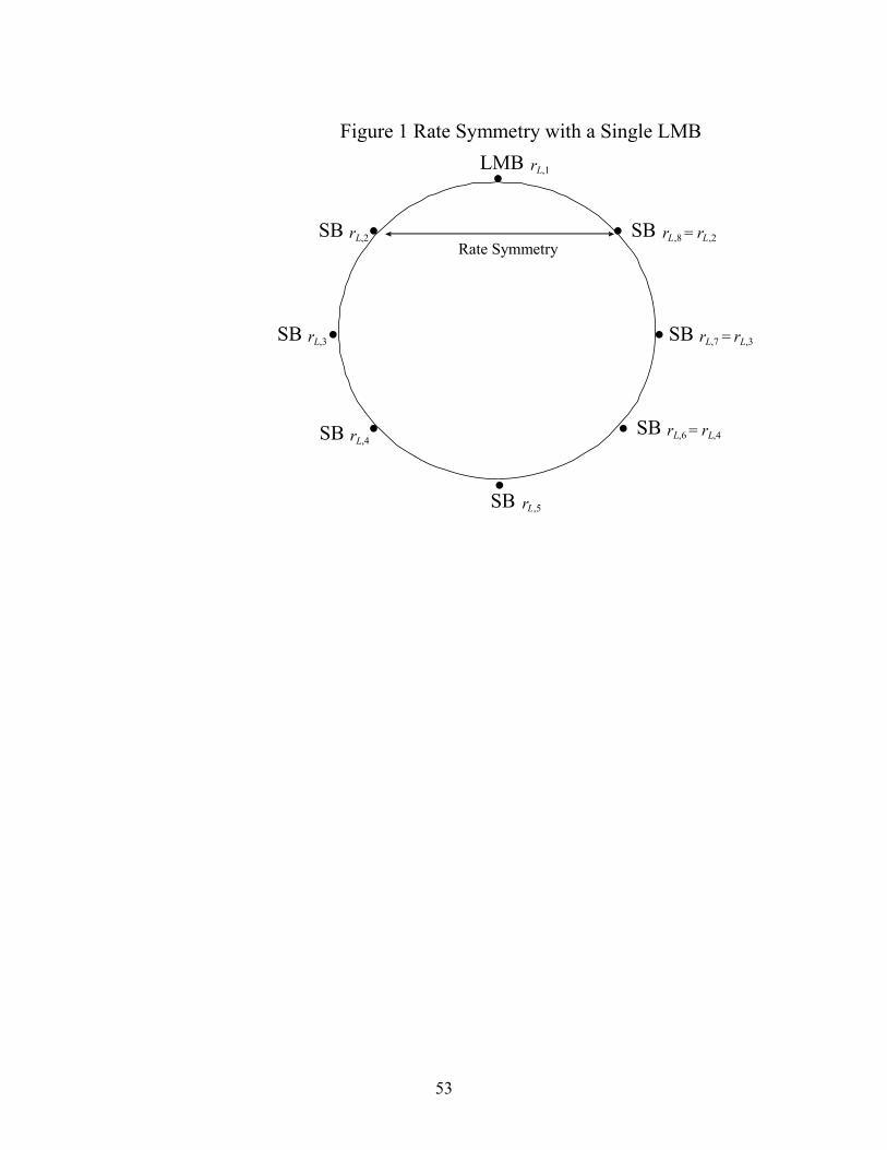
53

SB rL,5

•

•

•

•

• •

•

•

LMB rL,1

SB r L ,7 = rL,3SB r L ,3

SB r L,2

SB r L,4

SB r L ,8 = rL ,2

SB r L ,6 = r L,4

Figure 1 Rate Symmetry with a Single LMB

Rate Symmetry

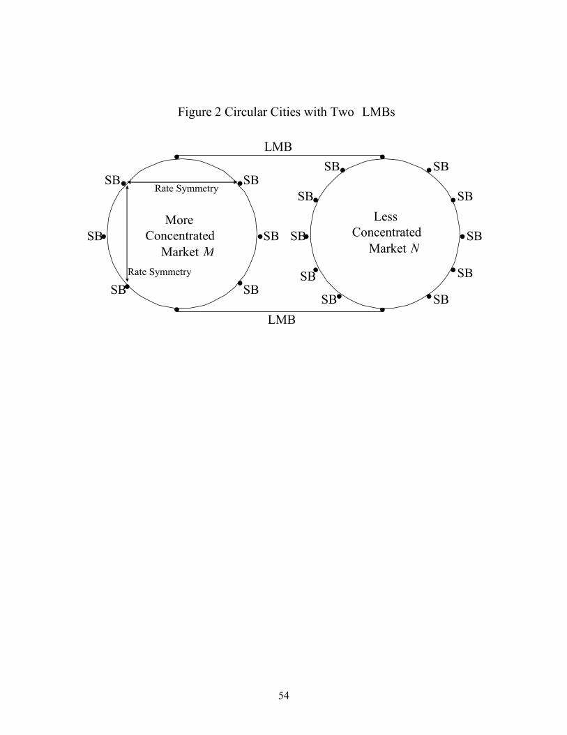
54

More Concentrated

Market M

MoreConcentrated

Market

LMB•

•

•

•

••

•

•

•

•

•

•SB

SB

SB

SB

SB

SB

SB

SBSB SBLess

ConcentratedMarket N

LMB

•

•

•

•

•

•

SB

SB

SB

SB

SB

•SB

•

•

Figure 2 Circular Cities with Two LMBs

Rate Symmetry

Rate Symmetry

55

Legends for Figures

Legend for Figure 1: Note: LMB indicates a large multimarket bank. SB indicates a small bank. Legend for Figure 2: Note: LMB indicates a large multimarket bank. SB indicates a small bank.

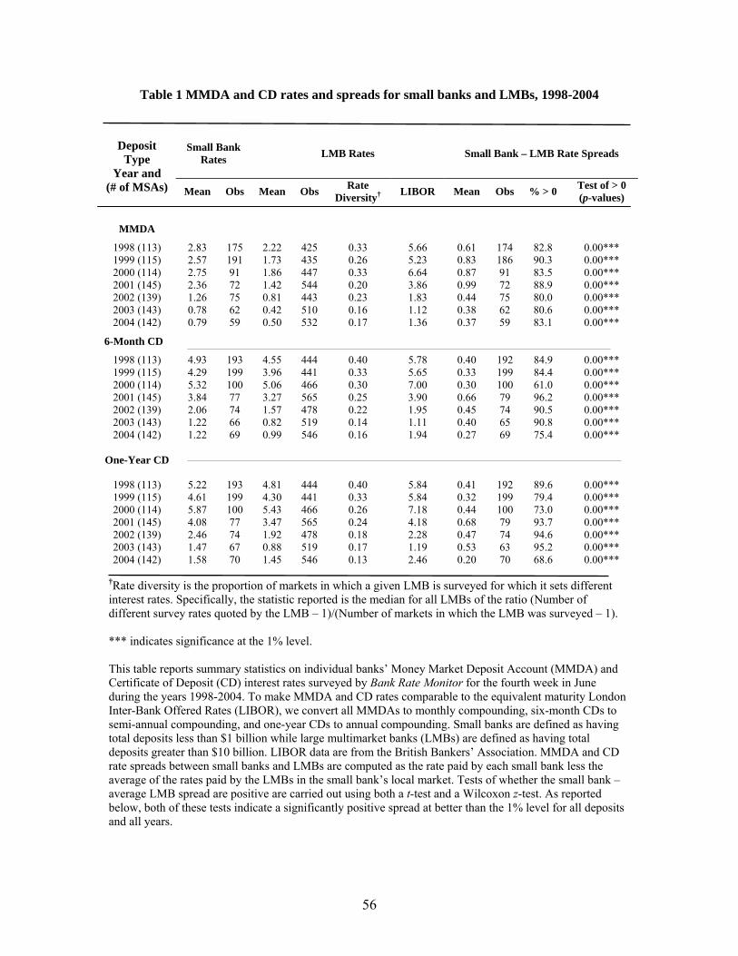
56

Table 1 MMDA and CD rates and spreads for small banks and LMBs, 1998-2004

Small Bank Rates LMB Rates Small Bank – LMB Rate Spreads

Deposit Type

Year and (# of MSAs) Mean Obs Mean Obs Rate

Diversity† LIBOR Mean Obs % > 0 Test of > 0 (p-values)

MMDA

1998 (113) 2.83 175 2.22 425 0.33 5.66 0.61 174 82.8 0.00*** 1999 (115) 2.57 191 1.73 435 0.26 5.23 0.83 186 90.3 0.00*** 2000 (114) 2.75 91 1.86 447 0.33 6.64 0.87 91 83.5 0.00*** 2001 (145) 2.36 72 1.42 544 0.20 3.86 0.99 72 88.9 0.00*** 2002 (139) 1.26 75 0.81 443 0.23 1.83 0.44 75 80.0 0.00*** 2003 (143) 0.78 62 0.42 510 0.16 1.12 0.38 62 80.6 0.00*** 2004 (142) 0.79 59 0.50 532 0.17 1.36 0.37 59 83.1 0.00***

6-Month CD 1998 (113) 4.93 193 4.55 444 0.40 5.78 0.40 192 84.9 0.00*** 1999 (115) 4.29 199 3.96 441 0.33 5.65 0.33 199 84.4 0.00*** 2000 (114) 5.32 100 5.06 466 0.30 7.00 0.30 100 61.0 0.00*** 2001 (145) 3.84 77 3.27 565 0.25 3.90 0.66 79 96.2 0.00*** 2002 (139) 2.06 74 1.57 478 0.22 1.95 0.45 74 90.5 0.00*** 2003 (143) 1.22 66 0.82 519 0.14 1.11 0.40 65 90.8 0.00*** 2004 (142) 1.22 69 0.99 546 0.16 1.94 0.27 69 75.4 0.00***

One-Year CD

1998 (113) 5.22 193 4.81 444 0.40 5.84 0.41 192 89.6 0.00*** 1999 (115) 4.61 199 4.30 441 0.33 5.84 0.32 199 79.4 0.00*** 2000 (114) 5.87 100 5.43 466 0.26 7.18 0.44 100 73.0 0.00*** 2001 (145) 4.08 77 3.47 565 0.24 4.18 0.68 79 93.7 0.00*** 2002 (139) 2.46 74 1.92 478 0.18 2.28 0.47 74 94.6 0.00*** 2003 (143) 1.47 67 0.88 519 0.17 1.19 0.53 63 95.2 0.00*** 2004 (142) 1.58 70 1.45 546 0.13 2.46 0.20 70 68.6 0.00***

†Rate diversity is the proportion of markets in which a given LMB is surveyed for which it sets different interest rates. Specifically, the statistic reported is the median for all LMBs of the ratio (Number of different survey rates quoted by the LMB – 1)/(Number of markets in which the LMB was surveyed – 1). *** indicates significance at the 1% level. This table reports summary statistics on individual banks’ Money Market Deposit Account (MMDA) and Certificate of Deposit (CD) interest rates surveyed by Bank Rate Monitor for the fourth week in June during the years 1998-2004. To make MMDA and CD rates comparable to the equivalent maturity London Inter-Bank Offered Rates (LIBOR), we convert all MMDAs to monthly compounding, six-month CDs to semi-annual compounding, and one-year CDs to annual compounding. Small banks are defined as having total deposits less than $1 billion while large multimarket banks (LMBs) are defined as having total deposits greater than $10 billion. LIBOR data are from the British Bankers’ Association. MMDA and CD rate spreads between small banks and LMBs are computed as the rate paid by each small bank less the average of the rates paid by the LMBs in the small bank’s local market. Tests of whether the small bank – average LMB spread are positive are carried out using both a t-test and a Wilcoxon z-test. As reported below, both of these tests indicate a significantly positive spread at better than the 1% level for all deposits and all years.

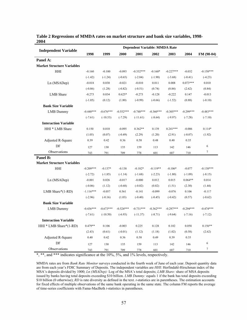
57

Table 2 Regressions of MMDA rates on market structure and bank size variables, 1998-2004

Dependent Variable: MMDA Rate Independent Variable

1998 1999 2000 2001 2002 2003 2004 FM (98-04)

Panel A:

Market Structure Variables

HHI -0.160 -0.100 -0.093 -0.332*** -0.160* -0.227*** -0.032 -0.158***

(-1.42) (-1.24) (-0.65) (-2.84) (-1.90) (-3.68) (-0.41) (-4.23)

Ln (MSADep) -0.018 0.030 -0.021 -0.010 0.011 0.008 0.073*** 0.010

(-0.86) (1.28) (-0.82) (-0.51) (0.74) (0.84) (2.62) (0.84)

LMB Share -0.273 0.034 0.625* -0.273 -0.128 -0.222 0.147 -0.013

(-1.05) (0.12) (1.80) (-0.99) (-0.66) (-1.52) (0.88) (-0.10)

Bank Size Variable

LMB Dummy -0.440*** -0.676*** -0.552*** -0.748*** -0.360*** -0.305*** -0.299*** -0.483***

(-7.61) (-10.53) (-7.29) (-11.61) (-8.64) (-9.97) (-7.28) (-7.10)

Interaction Variable

HHI * LMB Share 0.150 0.010 -0.095 0.362** 0.139 0.241*** -0.006 0.114*

(1.05) (0.07) (-0.49) (2.29) (1.20) (2.91) (-0.07) (1.92)

Adjusted R-Square 0.39 0.42 0.36 0.58 0.48 0.40 0.35

DF 127 130 135 159 113 142 146 6

Observations 743 791 709 778 601 687 710 7

Panel B: Market Structure Variables

HHI -0.209*** -0.137* -0.138 -0.182* -0.119** -0.106* -0.077 -0.138***

(-2.72) (-1.85) (-1.14) (-1.68) (-2.23) (-1.80) (-1.09) (-8.15)

Ln (MSADep) -0.001 0.026 -0.017 -0.000 0.012 0.015 0.064** 0.014

(-0.06) (1.12) (-0.68) (-0.02) (0.82) (1.51) (2.30) (1.44)

LMB Share*(1-RD) -1.116*** -0.057 0.561 -0.141 -0.099 -0.076 0.106 -0.117

(-2.96) (-0.16) (1.03) (-0.40) (-0.45) (-0.42) (0.57) (-0.62)

Bank Size Variable

LMB Dummy -0.436*** -0.673*** -0.524*** -0.731*** -0.362*** -0.297*** -0.294*** -0.474***

(-7.61) (-10.50) (-6.93) (-11.37) (-8.71) (-9.64) (-7.16) (-7.12)

Interaction Variable

HHI * LMB Share*(1-RD) 0.479** 0.106 -0.003 0.225 0.128 0.102 0.058 0.156**

(2.43) (0.61) (-0.01) (1.12) (1.18) (1.02) (0.58) (2.62)

Adjusted R-Square 0.40 0.42 0.36 0.58 0.49 0.39 0.35

DF 127 130 135 159 113 142 146 6

Observations 743 791 709 778 601 687 710 7

*, **, and *** indicates significance at the 10%, 5%, and 1% levels, respectively. MMDA rates are from Bank Rate Monitor surveys conducted in the fourth week of June of each year. Deposit quantity data are from each year’s FDIC Summary of Deposits. The independent variables are HHI: Herfindahl-Hirschman index of the MSA’s deposits divided by 1000; Ln (MSADep): Log of the MSA’s total deposits; LMB Share: share of MSA deposits issued by banks having total deposits exceeding $10 billion. LMB Dummy: equals 1 if the bank has total deposits exceeding $10 billion (0 otherwise); RD is rate diversity as defined in the text. t-statistics are in parentheses. The estimation accounts for fixed effects of multiple observations of the same bank operating in the same state. The column FM reports the average of time-series coefficients with Fama-MacBeth t-statistics in parentheses.

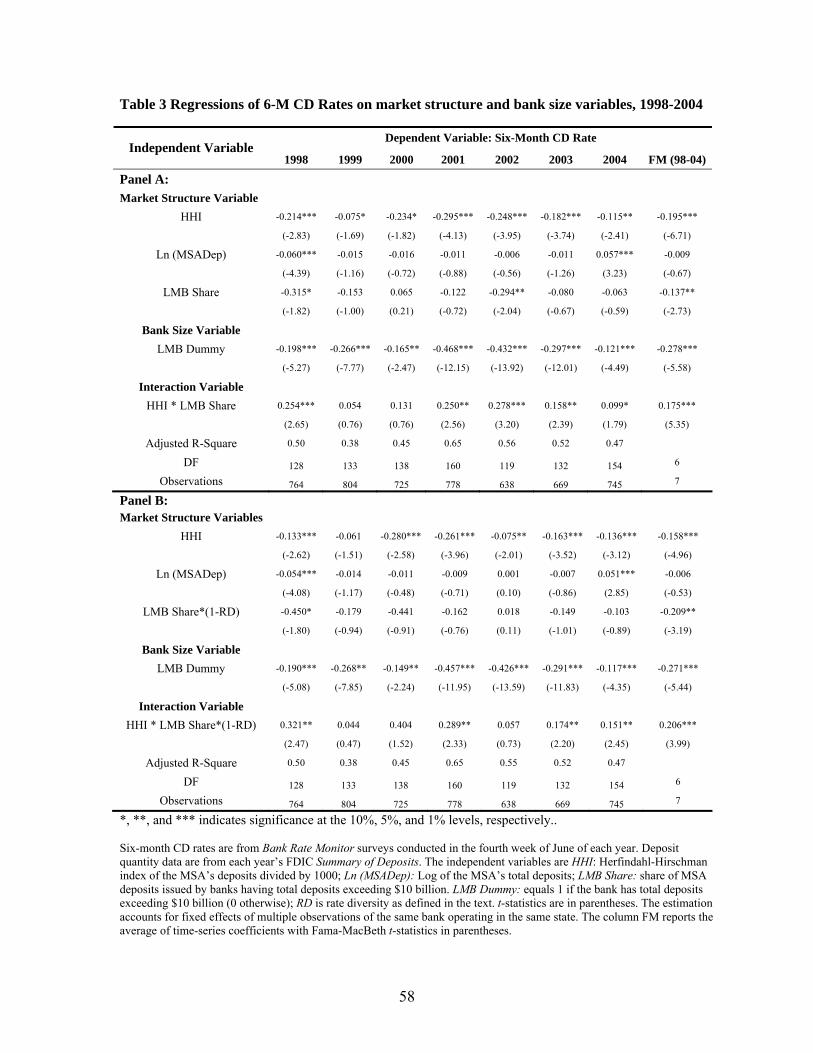
58

Table 3 Regressions of 6-M CD Rates on market structure and bank size variables, 1998-2004

Dependent Variable: Six-Month CD Rate Independent Variable

1998 1999 2000 2001 2002 2003 2004 FM (98-04)

Panel A:

Market Structure Variable

HHI -0.214*** -0.075* -0.234* -0.295*** -0.248*** -0.182*** -0.115** -0.195***

(-2.83) (-1.69) (-1.82) (-4.13) (-3.95) (-3.74) (-2.41) (-6.71)

Ln (MSADep) -0.060*** -0.015 -0.016 -0.011 -0.006 -0.011 0.057*** -0.009

(-4.39) (-1.16) (-0.72) (-0.88) (-0.56) (-1.26) (3.23) (-0.67)

LMB Share -0.315* -0.153 0.065 -0.122 -0.294** -0.080 -0.063 -0.137**

(-1.82) (-1.00) (0.21) (-0.72) (-2.04) (-0.67) (-0.59) (-2.73)

Bank Size Variable

LMB Dummy -0.198*** -0.266*** -0.165** -0.468*** -0.432*** -0.297*** -0.121*** -0.278***

(-5.27) (-7.77) (-2.47) (-12.15) (-13.92) (-12.01) (-4.49) (-5.58)

Interaction Variable

HHI * LMB Share 0.254*** 0.054 0.131 0.250** 0.278*** 0.158** 0.099* 0.175***

(2.65) (0.76) (0.76) (2.56) (3.20) (2.39) (1.79) (5.35)

Adjusted R-Square 0.50 0.38 0.45 0.65 0.56 0.52 0.47

DF 128 133 138 160 119 132 154 6

Observations 764 804 725 778 638 669 745 7

Panel B: Market Structure Variables

HHI -0.133*** -0.061 -0.280*** -0.261*** -0.075** -0.163*** -0.136*** -0.158***

(-2.62) (-1.51) (-2.58) (-3.96) (-2.01) (-3.52) (-3.12) (-4.96)

Ln (MSADep) -0.054*** -0.014 -0.011 -0.009 0.001 -0.007 0.051*** -0.006

(-4.08) (-1.17) (-0.48) (-0.71) (0.10) (-0.86) (2.85) (-0.53)

LMB Share*(1-RD) -0.450* -0.179 -0.441 -0.162 0.018 -0.149 -0.103 -0.209**

(-1.80) (-0.94) (-0.91) (-0.76) (0.11) (-1.01) (-0.89) (-3.19)

Bank Size Variable

LMB Dummy -0.190*** -0.268** -0.149** -0.457*** -0.426*** -0.291*** -0.117*** -0.271***

(-5.08) (-7.85) (-2.24) (-11.95) (-13.59) (-11.83) (-4.35) (-5.44)

Interaction Variable

HHI * LMB Share*(1-RD) 0.321** 0.044 0.404 0.289** 0.057 0.174** 0.151** 0.206***

(2.47) (0.47) (1.52) (2.33) (0.73) (2.20) (2.45) (3.99)

Adjusted R-Square 0.50 0.38 0.45 0.65 0.55 0.52 0.47

DF 128 133 138 160 119 132 154 6

Observations 764 804 725 778 638 669 745 7

*, **, and *** indicates significance at the 10%, 5%, and 1% levels, respectively.. Six-month CD rates are from Bank Rate Monitor surveys conducted in the fourth week of June of each year. Deposit quantity data are from each year’s FDIC Summary of Deposits. The independent variables are HHI: Herfindahl-Hirschman index of the MSA’s deposits divided by 1000; Ln (MSADep): Log of the MSA’s total deposits; LMB Share: share of MSA deposits issued by banks having total deposits exceeding $10 billion. LMB Dummy: equals 1 if the bank has total deposits exceeding $10 billion (0 otherwise); RD is rate diversity as defined in the text. t-statistics are in parentheses. The estimation accounts for fixed effects of multiple observations of the same bank operating in the same state. The column FM reports the average of time-series coefficients with Fama-MacBeth t-statistics in parentheses.

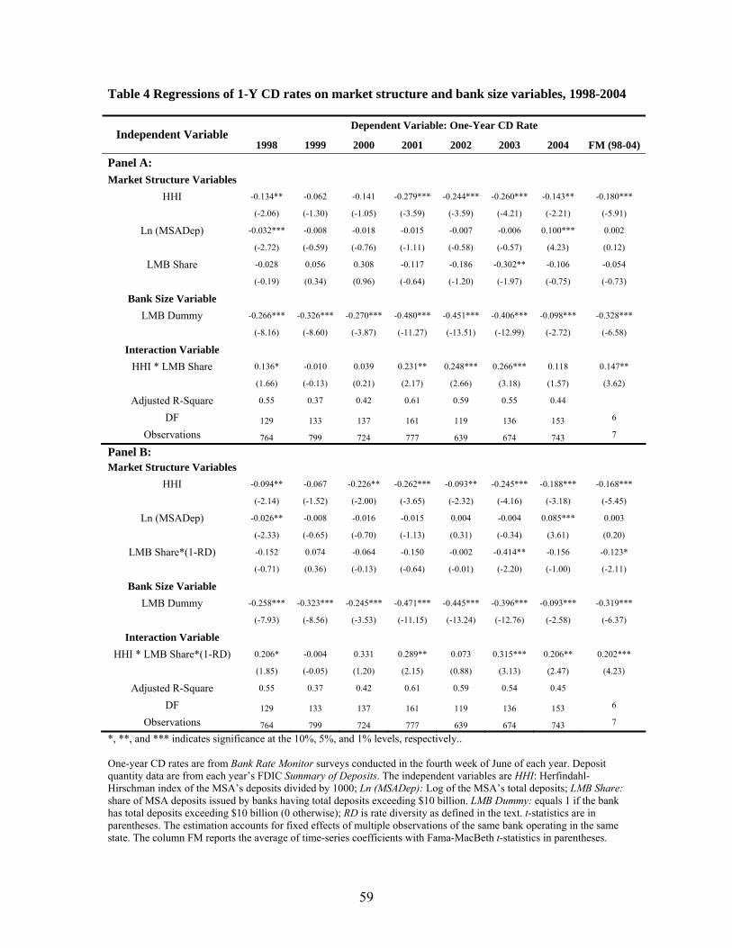
59

Table 4 Regressions of 1-Y CD rates on market structure and bank size variables, 1998-2004

Dependent Variable: One-Year CD Rate Independent Variable

1998 1999 2000 2001 2002 2003 2004 FM (98-04)

Panel A:

Market Structure Variables

HHI -0.134** -0.062 -0.141 -0.279*** -0.244*** -0.260*** -0.143** -0.180***

(-2.06) (-1.30) (-1.05) (-3.59) (-3.59) (-4.21) (-2.21) (-5.91)

Ln (MSADep) -0.032*** -0.008 -0.018 -0.015 -0.007 -0.006 0.100*** 0.002

(-2.72) (-0.59) (-0.76) (-1.11) (-0.58) (-0.57) (4.23) (0.12)

LMB Share -0.028 0.056 0.308 -0.117 -0.186 -0.302** -0.106 -0.054

(-0.19) (0.34) (0.96) (-0.64) (-1.20) (-1.97) (-0.75) (-0.73)

Bank Size Variable

LMB Dummy -0.266*** -0.326*** -0.270*** -0.480*** -0.451*** -0.406*** -0.098*** -0.328***

(-8.16) (-8.60) (-3.87) (-11.27) (-13.51) (-12.99) (-2.72) (-6.58)

Interaction Variable

HHI * LMB Share 0.136* -0.010 0.039 0.231** 0.248*** 0.266*** 0.118 0.147**

(1.66) (-0.13) (0.21) (2.17) (2.66) (3.18) (1.57) (3.62)

Adjusted R-Square 0.55 0.37 0.42 0.61 0.59 0.55 0.44

DF 129 133 137 161 119 136 153 6

Observations 764 799 724 777 639 674 743 7

Panel B: Market Structure Variables

HHI -0.094** -0.067 -0.226** -0.262*** -0.093** -0.245*** -0.188*** -0.168***

(-2.14) (-1.52) (-2.00) (-3.65) (-2.32) (-4.16) (-3.18) (-5.45)

Ln (MSADep) -0.026** -0.008 -0.016 -0.015 0.004 -0.004 0.085*** 0.003

(-2.33) (-0.65) (-0.70) (-1.13) (0.31) (-0.34) (3.61) (0.20)

LMB Share*(1-RD) -0.152 0.074 -0.064 -0.150 -0.002 -0.414** -0.156 -0.123*

(-0.71) (0.36) (-0.13) (-0.64) (-0.01) (-2.20) (-1.00) (-2.11)

Bank Size Variable

LMB Dummy -0.258*** -0.323*** -0.245*** -0.471*** -0.445*** -0.396*** -0.093*** -0.319***

(-7.93) (-8.56) (-3.53) (-11.15) (-13.24) (-12.76) (-2.58) (-6.37)

Interaction Variable

HHI * LMB Share*(1-RD) 0.206* -0.004 0.331 0.289** 0.073 0.315*** 0.206** 0.202***

(1.85) (-0.05) (1.20) (2.15) (0.88) (3.13) (2.47) (4.23)

Adjusted R-Square 0.55 0.37 0.42 0.61 0.59 0.54 0.45

DF 129 133 137 161 119 136 153 6

Observations 764 799 724 777 639 674 743 7

*, **, and *** indicates significance at the 10%, 5%, and 1% levels, respectively.. One-year CD rates are from Bank Rate Monitor surveys conducted in the fourth week of June of each year. Deposit quantity data are from each year’s FDIC Summary of Deposits. The independent variables are HHI: Herfindahl-Hirschman index of the MSA’s deposits divided by 1000; Ln (MSADep): Log of the MSA’s total deposits; LMB Share: share of MSA deposits issued by banks having total deposits exceeding $10 billion. LMB Dummy: equals 1 if the bank has total deposits exceeding $10 billion (0 otherwise); RD is rate diversity as defined in the text. t-statistics are in parentheses. The estimation accounts for fixed effects of multiple observations of the same bank operating in the same state. The column FM reports the average of time-series coefficients with Fama-MacBeth t-statistics in parentheses.

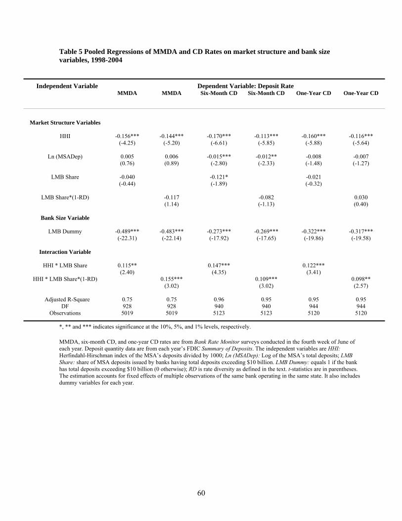
60

Table 5 Pooled Regressions of MMDA and CD Rates on market structure and bank size variables, 1998-2004

Independent Variable Dependent Variable: Deposit Rate

MMDA MMDA

Six-Month CD Six-Month CD

One-Year CD One-Year CD

Market Structure Variables

HHI -0.156*** (-4.25)

-0.144*** (-5.20)

-0.170*** (-6.61)

-0.113*** (-5.85)

-0.160*** (-5.88)

-0.116*** (-5.64)

Ln (MSADep) 0.005

(0.76) 0.006 (0.89)

-0.015*** (-2.80)

-0.012** (-2.33)

-0.008 (-1.48)

-0.007 (-1.27)

LMB Share -0.040

(-0.44) -0.121*

(-1.89) -0.021

(-0.32)

LMB Share*(1-RD) -0.117

(1.14) -0.082

(-1.13) 0.030

(0.40)

Bank Size Variable

LMB Dummy -0.489*** (-22.31)

-0.483*** (-22.14)

-0.273*** (-17.92)

-0.269*** (-17.65)

-0.322*** (-19.86)

-0.317*** (-19.58)

Interaction Variable

HHI * LMB Share 0.115**

(2.40) 0.147***

(4.35) 0.122***

(3.41)

HHI * LMB Share*(1-RD) 0.155*** (3.02)

0.109*** (3.02)

0.098** (2.57)

Adjusted R-Square 0.75 0.75 0.96 0.95 0.95 0.95

DF 928 928 940 940 944 944 Observations 5019 5019 5123 5123 5120 5120

*, ** and *** indicates significance at the 10%, 5%, and 1% levels, respectively. MMDA, six-month CD, and one-year CD rates are from Bank Rate Monitor surveys conducted in the fourth week of June of each year. Deposit quantity data are from each year’s FDIC Summary of Deposits. The independent variables are HHI: Herfindahl-Hirschman index of the MSA’s deposits divided by 1000; Ln (MSADep): Log of the MSA’s total deposits; LMB Share: share of MSA deposits issued by banks having total deposits exceeding $10 billion. LMB Dummy: equals 1 if the bank has total deposits exceeding $10 billion (0 otherwise); RD is rate diversity as defined in the text. t-statistics are in parentheses. The estimation accounts for fixed effects of multiple observations of the same bank operating in the same state. It also includes dummy variables for each year.

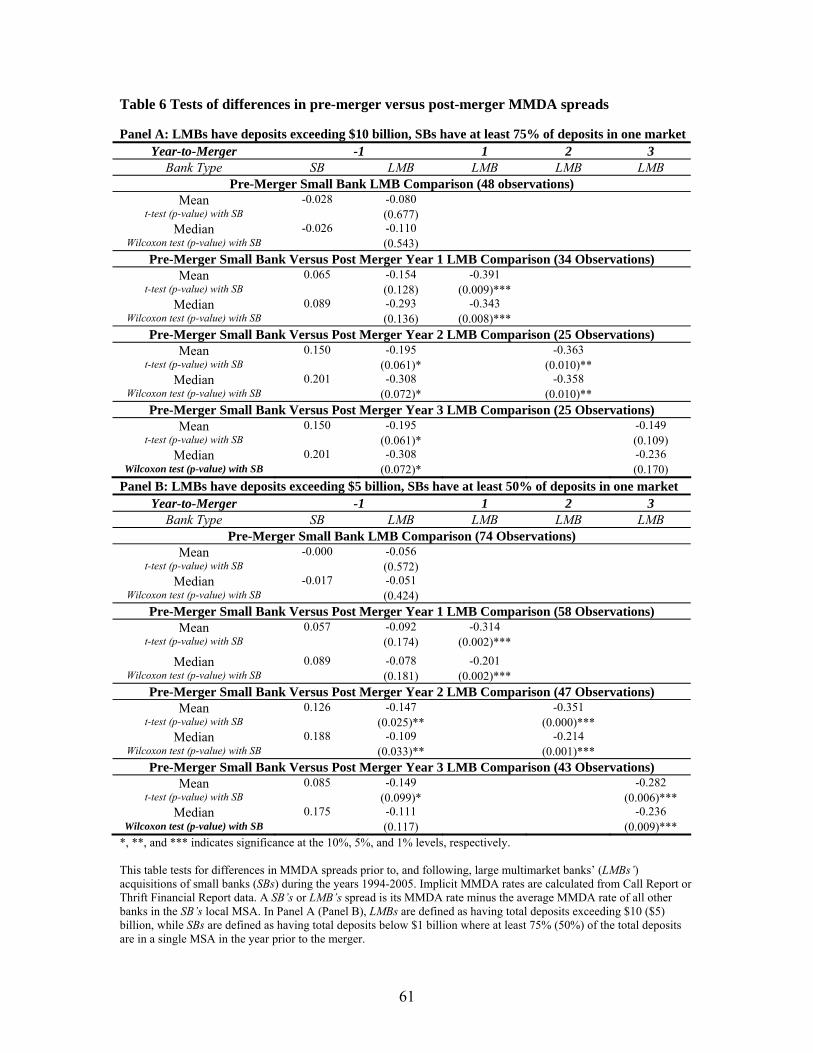
61

Table 6 Tests of differences in pre-merger versus post-merger MMDA spreads Panel A: LMBs have deposits exceeding $10 billion, SBs have at least 75% of deposits in one market

Year-to-Merger -1 1 2 3 Bank Type SB LMB LMB LMB LMB

Pre-Merger Small Bank LMB Comparison (48 observations) Mean -0.028 -0.080

t-test (p-value) with SB (0.677) Median -0.026 -0.110

Wilcoxon test (p-value) with SB (0.543) Pre-Merger Small Bank Versus Post Merger Year 1 LMB Comparison (34 Observations)

Mean 0.065 -0.154 -0.391 t-test (p-value) with SB (0.128) (0.009)***

Median 0.089 -0.293 -0.343 Wilcoxon test (p-value) with SB (0.136) (0.008)***

Pre-Merger Small Bank Versus Post Merger Year 2 LMB Comparison (25 Observations) Mean 0.150 -0.195 -0.363

t-test (p-value) with SB (0.061)* (0.010)** Median 0.201 -0.308 -0.358

Wilcoxon test (p-value) with SB (0.072)* (0.010)** Pre-Merger Small Bank Versus Post Merger Year 3 LMB Comparison (25 Observations)

Mean 0.150 -0.195 -0.149 t-test (p-value) with SB (0.061)* (0.109)

Median 0.201 -0.308 -0.236 Wilcoxon test (p-value) with SB (0.072)* (0.170)

Panel B: LMBs have deposits exceeding $5 billion, SBs have at least 50% of deposits in one market Year-to-Merger -1 1 2 3

Bank Type SB LMB LMB LMB LMB Pre-Merger Small Bank LMB Comparison (74 Observations)

Mean -0.000 -0.056 t-test (p-value) with SB (0.572)

Median -0.017 -0.051 Wilcoxon test (p-value) with SB (0.424)

Pre-Merger Small Bank Versus Post Merger Year 1 LMB Comparison (58 Observations) Mean 0.057 -0.092 -0.314

t-test (p-value) with SB (0.174) (0.002)***

Median 0.089 -0.078 -0.201 Wilcoxon test (p-value) with SB (0.181) (0.002)***

Pre-Merger Small Bank Versus Post Merger Year 2 LMB Comparison (47 Observations) Mean 0.126 -0.147 -0.351

t-test (p-value) with SB (0.025)** (0.000)*** Median 0.188 -0.109 -0.214

Wilcoxon test (p-value) with SB (0.033)** (0.001)*** Pre-Merger Small Bank Versus Post Merger Year 3 LMB Comparison (43 Observations)

Mean 0.085 -0.149 -0.282 t-test (p-value) with SB (0.099)* (0.006)***

Median 0.175 -0.111 -0.236 Wilcoxon test (p-value) with SB (0.117) (0.009)***

*, **, and *** indicates significance at the 10%, 5%, and 1% levels, respectively. This table tests for differences in MMDA spreads prior to, and following, large multimarket banks’ (LMBs’) acquisitions of small banks (SBs) during the years 1994-2005. Implicit MMDA rates are calculated from Call Report or Thrift Financial Report data. A SB’s or LMB’s spread is its MMDA rate minus the average MMDA rate of all other banks in the SB’s local MSA. In Panel A (Panel B), LMBs are defined as having total deposits exceeding $10 ($5) billion, while SBs are defined as having total deposits below $1 billion where at least 75% (50%) of the total deposits are in a single MSA in the year prior to the merger.