Hard scaling challenges for ab initio molecular dynamics
12
Journal of Physics: Conference Series OPEN ACCESS Hard scaling challenges for ab initio molecular dynamics capabilities in NWChem: Using 100,000 CPUs per second To cite this article: Eric J Bylaska et al 2009 J. Phys.: Conf. Ser. 180 012028 View the article online for updates and enhancements. You may also like Resolution-of-identity approach to Hartree–Fock, hybrid density functionals, RPA, MP2 and GW with numeric atom- centered orbital basis functions Xinguo Ren, Patrick Rinke, Volker Blum et al. - Physical origin of the one-quarter exact exchange in density functional theory Marco Bernardi - Interface dipoles of organic molecules on Ag(111) in hybrid density-functional theory Oliver T Hofmann, Viktor Atalla, Nikolaj Moll et al. - Recent citations From NWChem to NWChemEx: Evolving with the Computational Chemistry Landscape Karol Kowalski et al - Electron transfer calculations between edge sharing octahedra in hematite, goethite, and annite Eric J. Bylaska et al - Eric J. Bylaska et al - This content was downloaded from IP address 59.5.131.206 on 15/10/2021 at 08:02
Transcript of Hard scaling challenges for ab initio molecular dynamics

Journal of Physics Conference Series
OPEN ACCESS
Hard scaling challenges for ab initio moleculardynamics capabilities in NWChem Using 100000CPUs per secondTo cite this article Eric J Bylaska et al 2009 J Phys Conf Ser 180 012028
View the article online for updates and enhancements
You may also likeResolution-of-identity approach toHartreendashFock hybrid density functionalsRPA MP2 and GW with numeric atom-centered orbital basis functionsXinguo Ren Patrick Rinke Volker Blum etal
-
Physical origin of the one-quarter exactexchange in density functional theoryMarco Bernardi
-
Interface dipoles of organic molecules onAg(111) in hybrid density-functional theoryOliver T Hofmann Viktor Atalla NikolajMoll et al
-
Recent citationsFrom NWChem to NWChemEx Evolvingwith the Computational ChemistryLandscapeKarol Kowalski et al
-
Electron transfer calculations betweenedge sharing octahedra in hematitegoethite and anniteEric J Bylaska et al
-
Eric J Bylaska et al-
This content was downloaded from IP address 595131206 on 15102021 at 0802
Hard scaling challenges for ab initio molecular dynamics capabilities in NWChem Using 100000 CPUs per second
Eric J Bylaska1 Kevin Glass1 Doug Baxter1 Scott B Baden2 and John H Weare3
1 Environmental Molecular Sciences Laboratory Pacific Northwest National Laboratory PO Box 999 Richland WA 99354
2 Department of Computer Science and Engineering University of California San Diego 9500 Gilman Drive 0404 La Jolla CA 92093-0404
3 Department of Chemistry and Biochemistry University of California San Diego 9500 Gilman Drive 0303 La Jolla CA 92093-0303
Email EricBylaskapnlgov
Abstract An overview of the parallel algorithms for ab initio molecular dynamics (AIMD) used in the NWChem program package is presented including recent developments for computing exact exchange These algorithms make use of a two-dimensional processor geometry proposed by Gygi et al for use in AIMD algorithms Using this strategy a highly scalable algorithm for exact exchange has been developed and incorporated into AIMD This new algorithm for exact exchange employs an incomplete butterfly to overcome the bottleneck associated with exact exchange term and it makes judicious use of data replication Initial testing has shown that this algorithm can scale to over 20000 CPUs even for a modest size simulation
1 Introduction The ability to predict the properties of complex materials important in toxic waste disposal disease treatment efficient chemical processing and electronic device performance optimization among others is of great importance to DOErsquos efforts to address the nationrsquos energy and environmental problems Because the required properties are highly sensitive to complex interactions at the fundamental electronic structure level (eg chemical bond saturation shell structure) reliable parameter-free simulation of their properties requires methods based directly on the solution to the electronic structure problem posed by the electronic Schroumldinger equation Development of methods at the fundamental electronic structure level also is important in light of DOErsquos investment in large-scale facilities such as the synchrotron light and neutron sources These new probes are providing an unprecedented level of detail at the atomic and molecular scale However without appropriate theories or models many of these new measurements cannot be readily interpreted
SciDAC 2009 IOP PublishingJournal of Physics Conference Series 180 (2009) 012028 doi1010881742-65961801012028
ccopy 2009 IOP Publishing Ltd 1
The method of ab initio molecular dynamics (AIMD) enables researchers to treat the dynamics of
these systems while retaining a first-principles-based description of their interactions [3-8] This approach is similar to classical molecular dynamics where the motions of the atoms and molecules are simulated over a period of time but here the interactions between the atoms are calculated directly from the electronic Schroumldinger equation rather than from empirical interaction potentials or force fields That is at every step of a molecular dynamics simulation the locations of the electrons in the atoms and molecules are determined by solving a suitable approximation to the electronic Schroumldinger equation The instantaneous forces on the atoms are then determined by calculating their electrostatic forces from their interaction with other ions and electrons in the system
An example of the use of AIMD simulations is for the study of hydrated radionuclides under extreme conditions A major obstacle to the development of nuclear power is the ability to safely store highly dangerous waste materials containing uranium and other radionuclides [9-11] Most current storage strategies are designed to store waste in saturated and unsaturated geological formations [12-15] Stored in this way the most likely means for uranium to migrate into the biosphere is through groundwater contact with containment canisters resulting in a solvated UO2
2+ cation (or complexes) [12] To reliably predict behavior of the radionuclide (eg uranium thorium and plutonium) waste products of nuclear power production over the range of conditions encountered in a storage facility requires a theory based at the most fundamental level on the electronic Schroumldinger equation In figure 1 results from a recent AIMD simulation of the UO2
2+ cation in aqueous solution are shown [2] Even though the UO2
2+ cation has been studied extensively over the years using a variety of static ab initio (eg static coupled cluster calculations) and classical molecular dynamics methods these prior simulations either have been incomplete or inaccurate Static ab initio simulations have been incomplete because they were not able to take into account the motion of the water molecules in the second and apical solvent shells and classical molecular dynamic simulations have been plagued by inaccurate force fields of the complex interactions between the UO2
2+ cation and water AIMD simulations which are able to take into account complex interactions and dynamics are able overcome the well-known deficiencies of other molecular simulation methods In fact this AIMD simulation was the first molecular simulation able to reproduce the measured Extended X-ray Absorption Fine Structure (EXAFS) spectrum from experiments
Because the electronic Schroumldinger equation is solved at every step in the simulation this type of simulation requires an enormous amount of computational power The typical time-step in an AIMD simulation is quite small (~01 femtosecond=10-16 seconds) and the simulations needs to run at least 10 picoseconds Many chemical processes of interest occur on the order of nanoseconds (10-9 seconds) Even for a 10 picosecond AIMD simulation at least 10-1110-16=105 evaluations of the electronic
Figure 1 The experimental [1] and simulated extended x-ray absorption fine structure spectra of UO2
2+ in water are in perfect agreement (left) On the right a snapshot of the inner solvation shell UO2
2+ is shown The blue surface identifies the inner-coordination spheres and golden lines show the array of hydrogen bonds that are formed in the structure The results shown are from NWChem ab initio molecular dynamics simulation of UO2
2+ and 122 H2O molecules [2]
SciDAC 2009 IOP PublishingJournal of Physics Conference Series 180 (2009) 012028 doi1010881742-65961801012028
2
Schroumldinger equation are needed Compared to merely optimizing a molecular or solid-state structure which requires at most a few hundred evaluations this is extremely expensive In order for this to be a practical method the solution to the electronic Schroumldinger equation in a single time-step must be able to complete within seconds For example the computational time needed to simulate 100 picoseconds will be 115 days with a single time-step taking 1 second to complete 115 days with a 10 second time-step and ~1 year with a 30 second time-step In general for systems beyond a few atoms even the least expensive approximations to the electronic Schroumldinger equation are expensive to calculate
With the advent of massively parallel computers and the development of new parallel algorithms and software the costs of AIMD are becoming manageable Scalable implementations of AIMD began appearing on hundreds of processors in the early to mid 1990rsquos [16-18] and improvements continue to this day [19-22] Notably (Gordon Bell Prize) F Gygi et al [22] have scaled a band structure calculation on 64K nodes of Blue Gene L using the Qbox FPMD code
The most popular approximation to the electronic Schroumldinger equations used for AIMD today is Density Functional Theory (DFT) based on computationally efficient approximations to the exact exchange-correlation functional (eg LDA and GGA) While this level of approximation is suitable for many applications it is also becoming clear that higher levels of exchange-correlation potential that are augmented with some fraction of exact exchange (hybrid-DFT eg PBE0 [23]) are needed The lower levels of exchange correlation potentials presently used in AIMD simulation software are unable to reliably predict the properties of many materials in basic research Examples of interest to DOE include charge localization in transition elements with tightly bound d electrons in oxide materials (see figure 2) [24 25] the underestimation of reaction barriers and band gaps in solids [26-28] and accurate predictions of spin structure of solids [29] and nanoparticles The drawback of hybrid-DFT is that it adds a significant amount of expense to an already expensive AIMD simulation Until recently it was infeasible to contemplate such computations However as we approach the Petaflop milestone we can think about coping with the high computational costs through vastly increased parallelism
In this study we present an overview of the parallel algorithms for AIMD used in the NWChem program package [30] including recent developments for computing exact exchange [31] These algorithms make use of a two-dimensional processor geometry proposed by Gygi et al for use in AIMD algorithms Using this strategy we have recently developed a highly scalable algorithm for exact exchange and incorporated it into an AIMD application This new algorithm for exact exchange employs an incomplete butterfly to overcome the bottleneck associated with exact exchange term and makes judicious use of data replication
2 Key computations in AIMD The bulk of the computations in ab initio molecular dynamics (AIMD) algorithms revolves around the solution of Ne weakly nonlinear partial differential eigenvalue equations (PDEs) Hψi = εiψi for the electron orbitals ψi appearing as a result of the DFT approximation to the Schroumldinger equation for an Ne electron system Generally only the Ne lowest eigenfunctions are required Most standard AIMD algorithms use non-local pseudopotentials and plane-wave basis sets to perform the DFT calculations In this framework solutions are typically approached by means of a conjugate gradient algorithm or
Figure 2 Illustration of a localized electron (ie polaron) on the surface of hematite calculated with a higher and more expensive level (eg hybrid DFT) of ab initio molecular dynamics Lower levels of ab initio molecular dynamics will predict a delocalized electron
SciDAC 2009 IOP PublishingJournal of Physics Conference Series 180 (2009) 012028 doi1010881742-65961801012028
3
Figure 3 Operation count of Hψ in a plane-wave DFT simulation
for dynamics a Car-Parrinello algorithm [3] that requires many evaluations of Hψi along with maintaining orthogonality
( ) ( ) jiji d δψψ =intΩrrr (1)
Similar FFT-based solution methods are implemented in a number of widely distributed first principles simulation software packages eg NWChem [30]
For hybrid-DFT the Hamiltonian operator H may be written as [32]
Hψ i r( )=minus
12
nabla2 + Vl r( )+ ˆ V NL + VH ρ[ ] r( )
+ 1minusα( )Vx ρ[ ] r( )+ Vc ρ[ ] r( )
⎛
⎝
⎜ ⎜ ⎜
⎞
⎠
⎟ ⎟ ⎟ ψ i r( )minusα Kij r( )ψ j r( )
jsum (2)
where the one electron density is given by
ρ r( )= ψi r( )2
i=1
Ne
sum (3)
The local and non-local pseudpootentials Vl and VNL represent the electron-ion interaction The Hartree potential VH is given by
nabla 2VH r( )= minus4πρ r( ) (4) The local exchange and correlation potentials are Vx and Vc and exact exchange kernels Kij are given by
nabla2Kij r( )= minus4πψ j r( )ψ i r( ) (5)
During the course of a total energy minimization or AIMD simulation the electron gradient Hψi (equation (2)) and orthogonalization (equation (1)) are evaluated many times (ie gt10000 for AIMD)
and hence need to be calculated as efficiently as possible For a pseudopotential plane-wave calculation the main parameters that determine the cost of a of the electron gradient are Ng Ne Na and Nproj where Ng is the size of the three-dimensional FFT grid Ne is the number of occupied orbitals Na is the number of atoms and Nproj is the number of projectors per atom Summaries of the computational costs for each of the constituent parts of electron
gradient (and orthogonality) are given in figure 3 The major parts of the electron gradient in order of increasing asymptotic cost are (note that conventional DFT does not compute the exact exchange term α = 0 in equation (2))
bull The Hartree potential VH including the local exchange and correlation potentials Vx+Vc The main computational kernel in these computations is the calculation of Ne three-dimensional FFTs
bull The non-local pseudopotential VNL The major computational kernel in this computation can be expressed by the following matrix multiplications W = PtY and Y2 =PW where P is an Ng x (NprojNa) matrix Y and Y2 are Ng x Ne matrices and W is an (NprojNa) x Ne matrix We note that for most pseudopotential plane-wave calculations NprojNaasympNe
bull Enforcing orthogonality The major computational kernels in this computation are following matrix multiplications S=YtY and Y2 = YS where Y and Y2 are Ng x Ne matrices and S is an Ne x Ne matrix
SciDAC 2009 IOP PublishingJournal of Physics Conference Series 180 (2009) 012028 doi1010881742-65961801012028
4
bull And when exact exchange is included the exact exchange operator ΣKijψj The major computational kernel in this computation involves the calculation of (Ne+1)Ne three-dimensional FFTs The computation of the exact exchange operator in which O(Ne
2) independent Poisson equations must be solved is by far the most demanding term in a pseudopotential plane-wave hybrid-DFT calculation
3 Parallelization of AIMD (wo exact exchange) There are several ways to parallelize a plane-wave Hartree-Fock and DFT program [7 17 18 22 33 34] For many solid-state calculations the computation can be distributed over the Brillouin zone sampling space [33] This approach is very simple to implement however it cannot be used for Γ-point (k=0) calculations with large unit cells Another approach is to distribute the one-electron orbitals across processors [17] The drawback of this method is that orthogonality will involve a lot of message passing Furthermore this method will not work for simulations with very large cutoff energy requirements (ie using large numbers of plane-waves to describe the one-electron orbitals) on parallel computers that have nodes with a small amount of memory because a complete one-electron must be stored on each node Hence this approach is not practical for Car-Parrinello simulations with large unit cells however this approach can work well for simulations with modest size unit cells and with small cutoff energies when used in combination with minimization algorithms that perform orthogonalization sparingly eg RMM-DIIS [6 35]
Another straightforward way parallelize AIMD is to spatially decompose the one-electron orbitals [7 18 34] This approach is versatile easily implemented and well suited for performing Car-Parrinello simulations with large unit cells and cutoff energies Moreover the parallel implementation of the non-local pseudopotential and orthogonality is very easy to implement since they can be implemented using the simple global operation reduce The drawback of this approach is that a parallel three-dimensional fast Fourier transform (FFT) must be used which is known not to scale beyond ~Ng
13 CPUs (or processor groups) where Ng is the number of FFT grid points In figure 4 an example of timings versus the number of CPUs for this type of parallelization is
shown These simulations were taken from a Car-Parrinello simulation of UO2
2++122H2O with an FFT grid of Ng=963 (Ne=1000) using the plane-wave DFT module (PSPW) in NWChem [30] These calculations were performed on all four cores on the quad-core Cray-XT4 system (NERSC Franklin) composed of a 23 GHz single socket quad-core AMD Opteron processors (Budapest) The NWChem program was compiled using Portland Group FORTRAN 90 compiler version 724 and linked with the Cray MPICH2 library version 302 for message passing The performance of the program is reasonable with an overall parallel efficiency of 84 on 128 CPUs dropping to 26 by 1024 CPUs However not every part the program scales in exactly the same way For illustrative purposes the timings of the FFTs non-local pseudopotential and orthogonality are also shown The parallel efficiency of the FFTs is by far the worst of the three major parts of the computation Beyond 100 CPUs no gainful work was found in the FFT computation However at smaller CPU sizes the inefficiency of the FFTs are damped out due to the fact that these parts of the code make up less than 5 of the overall computation and the largest part of the
Figure 4 Overall and component timings and component from AIMD simulations of UO2
2++122H2O using 1d processor geometry Overall best timings also shown for 2d processor geometry Timings from calculations on the Franklin Cray-XT4 computer system at NERSC
SciDAC 2009 IOP PublishingJournal of Physics Conference Series 180 (2009) 012028 doi1010881742-65961801012028
5
1d and 2d Processor Geometries
Ngrid=N1xN2xN3
Norbitals
Ngrid=N1xN2xN3
Norbitals
Ngrid=N1xN2xN3
Norbitals
Ngrid=N1xN2xN3
Norbitals
Figure 5 A parallel distribution (shown on the left) implemented in most plane-wave DFT software each of the one-electron orbitals is identically spatially decomposed The 2d parallel distribution suggested by Gygi et al is shown on the right
calculation is the non-local pseudopotential evaluation Ultimately however the lack of scalability of the 3D FFT algorithm beyond ~Ng
13 CPUs prevails and the simulation ceases to speedup By 1000 CPUs the non-local pseudopotential has also stalled Interestingly at this number of CPUs the costs of the non-local pseudopotential and the FFTs are roughly the same Only orthogonality continues to scale beyond 1000 CPUs
These results demonstrate an important guiding principle that is needed in the design of a parallel AIMD program The number of CPUs that can be gainfully used in each of the major parts of the calculation is limited because they rely on global operations or all to all operations that use all CPUs in the calculation Hence the overall parallel algorithm
for AIMD should be designed to avoid global communications that span all CPUs in the calculation For example Gygi et al distribute across orbitals as well as over space [22] resulting in a in a 2d processor geometry as shown in figure 5 (where the total number of processors Np can be written as Np=NpiNpj) This decomposition reduces the cost of the global operations in the major parts of the electron gradient computation which only need O(log Npi) or O(log Npj) communications per CPU instead of O(log Np) For example the FFT and non-local pseudopotential tasks only need to use global operations that span over Npi while the orthogonality step can be broken down into a series of alternating global operations that span over either Npi or Npj eg like the SUMMA algorithm [36]
The overall performance of our AIMD simulations was found to improve considerably using this new approach With the optimal processor geometries the running time per step took 2699 seconds (45 minutes) for 1 CPUs down to 37 seconds with a 70 parallel efficiency on 1024 CPUs The fastest running time found was 18 seconds with 36 parallel efficiency on 4096 CPUs As shown in figure 6 these timings were found to be very sensitive to the layout of the two-dimensional processor geometry For 256 512 1024 and 2048 CPUs the optimal processor geometries were 64x4 64x8 128x8 and 128x16 processor grids respectively The timings of the FFTs non-local pseudopotential and orthogonality are also shown in figure 6 Not every part the program scaled perfectly The parallel efficiency of several other key operations depends strongly on the shape of the processor geometry It was found that distributing the processors over the orbitals significantly improved the efficiency of the FFTs and the non-local pseudopotential while distributing the processors over the spatial dimensions favored the orthogonality computations
Figure 6 Overall and component timings in seconds for UO2
2++122H2O plane-wave DFT simulations at various processor sizes (Np) and processor grids (Npj Npi=NpNpj) Timings were determined from calculations on the Franklin Cray-XT4 computer system at NERSC
SciDAC 2009 IOP PublishingJournal of Physics Conference Series 180 (2009) 012028 doi1010881742-65961801012028
6
4 Parallelization of AIMD with exact exchange The 2d processor geometry method can also be used to parallelize the computation of the exact exchange operator This operator has a cost of O(Ne
2Nglog(Ng)) and when it is included in a plane-wave DFT calculation it is by far the most demanding term The exchange term is well suited for this method whereas if only the spatial or orbital dimensions are distributed then the exchange term does not scale well When only the spatial dimensions are distributed each of the Ne(Ne+1) 3d FFTs will be computed one at a time on the entire machine The drawback of this approach is that it significantly underutilizes the resources since parallel efficiency of a single 3d FFT is effectively bounded to ~Ng
13 processors When only the orbital dimensions are distributed the parallelization is realized by multicasting the O(Ne) orbitals to set up the O(Ne
2) wave-function pairs This multicast is followed by a multi-reduction which reverses the pattern We note that with this type of algorithm one could readily fill a very large parallel machine by assigning each a few FFTs to each processor However in order to obtain reasonable performance from this algorithm it is vital to mask latency since the interconnects between the processors will be flooded with O(Ne) streams each on long messages comprising Ng floating point words of data In which both the spatial and orbital dimensions are distributed we only need to compute parallel three-dimension FFTs along the processor grid columns as well as broadcast the orbitals along the processor grid rows Compared with a multicast across all processors the benefit of this approach is to reduce latency costs since broadcasting is done across the rows of the two-dimensional processor grid only The basic steps involved in calculating the exchange operator with this distribution are given in the following algorithm
Basic parallel algorithm for calculating exact exchange in a plane-wave basis using a 2d processor geometry Input ψ - (NgNpi) x (NeNpj) array Output Kψ -(NgNpi) x (NeNpj) array Work Space Ψ ndash (NgNpi) x Ne array KΨ ndash (NgNpi) x Ne array Ne = total number of orbitals Np = total number of processors where Np=NpiNpj Npi Npj = size of column (row) processor group taskid_ij = rank along the column (row) processor group Ψ() ΚΨ () = 0 s=taskid_j(NeNpj) e = s+(NeNpj)Ψ(se) = ψ Row_Reduction(Ψ) counter = 0 for m=1Ne for n=1m if counter==taskid_j then ρ() Column_FFT_rc( (Ψ(m) Ψ(n)) ) V() Column_FFT_cr( (fscreened() ρ()) ) KΨ(m ) -=V()Ψ(n) if m = n then KΨ(n) -=V()Ψ(m) end if end if counter = mod(counter + 1Npj) end for end for Row_Reduction(KΨ) Kψ=HΨ(se)
In this algorithm the routines Column_FFT_rc and Column_FFT_cr are the forward and
reverse parallel three-dimensional Fast Fourier Transforms (FFTs) along the processor columns
SciDAC 2009 IOP PublishingJournal of Physics Conference Series 180 (2009) 012028 doi1010881742-65961801012028
7
Row_Reduction is a parallel reduction along the processor rows and fscreened is the cutoff of Coulomb kernel given by the Fourier transform of the following real-space function
( ) ( ) ( )r
RrrfNNexp11 minusminusminus
= (6)
where R and N are adjustable parameters [24 31 37] This algorithm is very simple to implement and it is perfectly load balanced since each CPU only computes (Ne(Ne+1)Np) three-dimension FFTs However this simple algorithm can be improved One problem with it is that it uses a lot of workspace Another is that each CPU in the Row_Reduction subroutine receives and sends a total of (Npj-1)(NgNpi)(NeNpj)~=NgNeNpi amount of data which is approximately twice as much as is necessary to compute all pairs of wave functions We have recently developed a slightly more ambitious parallel algorithm for calculating the exchange operator which halves the workspace and communication overhead while maintaining a good load balance The key idea behind this algorithm is that a specially designed broadcast and reduce routines are called that basically implement a standard asynchronous radix-2 butterfly diagram except that instead of transferring a (Npj2)NgNeNp chunk of data at the last step they transfer only a (NgNpi)(NeNpj)(1+(Npj-2Floor(Log2(Npj))))~=NgNeNp chunk data
The overall best timings for hybrid-DFT calculations of an 80 atom supercell of hematite (Fe2O3) with an FFT grid of Ng=723 (Ne
up=272 Nedown=272) and a 160 atom supercell of hematite (Fe2O3) with
an FFT grid of Ng=144x72x72 (Neup=544 and Ne
down=544) (wavefunction cutoff energy=100Ry and density cutoff energy=200Ry) and orbital occupations of Ne
up=272 and Nedown=272 are shown in figure
7 The overall best timing per step found for the 80 atom supercell was 36 seconds on 9792 CPUs and for the 160 atom supercell of hematite was 177 seconds on 23936 CPUs The timings results are somewhat uneven since limited numbers of processor grids were tried at each processor size However even with this limited amount of sampling these calculations were found to have speedups to at least 25000 CPUs We expect that further improvements will be obtained by trying more processor geometry layouts
The time to compute the exchange operator using can be broken up into two parts the time to compute the Ne(Ne+1) three-dimensional FFTs (tfft) and the time to perform the data transfer (tbutterfly) in the Brdcst_Step and Reduce_Step subroutines ie
butterflyfftexchange ttt += (7)
The three-dimensional parallel FFT in the NWChem program packages uses a two-dimensional Hilbert decomposition of the three-dimensional FFT grid [5] For this type of FFT the time to compute one three-dimensional FFT can be approximated by summing up three terms corresponding to serial computational data transfer and latency times
NpiNpi
NNpi
NLogNat ggg
fft θγ
22)( 21 ++=
(8) where Ng is the size of the FFT grid Npi is the
number of rows in the two-dimensional processor grid and a θ γ are adjustable parameters corresponding to the rate to compute one 3d FFT in serial θ is the
Figure 7 The overall fastest timings taken for an 80 and 160 atom Fe2O3 hybrid-DFT energy calculations Timings from calculations on the Franklin Cray-XT4 computer system at NERSC
SciDAC 2009 IOP PublishingJournal of Physics Conference Series 180 (2009) 012028 doi1010881742-65961801012028
8
effective latency to start a message and γ is the effective rate to transfer a message
For each incomplete butterfly broadcast and reduction the bandwidth part of the data transfer per CPU will be proportional to (Npj2)(NgNpi)(NeNpj) or (12)(NeNgNpi) and the number of messages per CPU will be proportional Log2(Npj) Thus the overall timing for performing the data transfer can be written as
)(4)21(4 2 NpjLogNpi
NNt eg
butterfly θγ += (9)
The extra factor of 4 is due to the fact that both Log2(Npj) broadcast and reductions steps are performed and each broadcast and reduction step contains a send and a receive call
By combining equations (7-9) we arrive at the following equation for the time to compute the exchange operator
)(4
)21(4
)1(
2
1
NpjLogNpi
NN
tNpjNNt
eg
fftee
exchange
θ
γ
+
+
+=
(10)
From an approximate fitting of the model to the 80 Fe2O3 simulation atom simulation the parameters were found to be a=4e-9 θ=25e-4 and γ=5e-8 (see figure 8) As shown in figure 4 the fastest execution time will be obtained when Npj=Ne From this relation the maximum number of CPUs can be readily estimated by solving the following equation
0==NeNpj
exchange
dNpidt
(11)
for Npi The solution to equation (11) is then 322max ⎟
⎠⎞
⎜⎝⎛=
BANpi (12)
where
( ) ⎟⎟⎠
⎞⎜⎜⎝
⎛ ++++=
e
eeggge N
NNNNNNaA 112)(log1 2 γ (13)
( )θ12 += eNB (14) Using this formula we find that the maximum number of CPUs that can be gainfully used in the 80
and 160 atom Fe2O3 Hybrid-DFT calculations to be 14977 CPUs and 48032 CPUs respectively and we plan to validate these results in the future
5 Conclusion An overview of the parallel algorithms used for AIMD in the NWChem program package is presented including recent developments for computing exact exchange These algorithms were based on using a two dimensional processor geometry which allowed us to overcome the inefficiencies associated with
Figure 8 Comparison of performance model with measured timings for 80 atom Fe2O3 hybrid DFT calculation (a=4e-9 θ=25e-4 and γ=5e-8)
SciDAC 2009 IOP PublishingJournal of Physics Conference Series 180 (2009) 012028 doi1010881742-65961801012028
9
using parallel three-dimensional FFTs A unique aspect of our implementation of exact exchange is the development of an incomplete butterfly that halves the amount of data communicated as well as making judicious use of data replication in the exact exchange compared to a standard multicast algorithm
The overall performances of our AIMD calculations were found to be fairly reasonable For a UO2
2++122H2O AIMD simulation the running time per step decreased from 2699 seconds (45 minutes) for 1 CPUs down to 37 seconds with a 70 parallel efficiency on 1024 CPUs The fastest running time found was 18 seconds with 36 parallel efficiency on 4096 CPUs For an 80 atom Fe2O3 hybrid- DFT AIMD simulation the overall parallel efficiency to 1024 processors was 99 decreasing to 53 by 9792 processors Beyond 10000 processors no speedups were observed for this calculation and larger systems are required if we are to use higher levels of parallelism Limited simulations for a larger 160 atom Fe2O3 hybrid-DFT AIMD simulations were also carried out These calculations did not produce as good parallel efficiencies as the 80 atom simulations however these calculations were found to have speedups to at least 25000 CPUs We believe the communications overheads are still an issue and we are exploring latency hiding techniques via run time substrates that implement a dataflow execution model [38-40]
Significant progress has been made in terms of accuracy efficiency and scalability of AIMD methods in recent years However the algorithms and implementations of these methods need to be constantly upgraded to capture the performance of emerging massively parallel computers The projected size of the next generation supercomputers are very large (106-107 threads of computation) suggesting that current limitations in simulation times particle sizes and levels of theory will be overcome in the coming years by brute force increases in computer size
6 Acknowledgements This research was partially supported by the ASCR Multiscale Mathematics program the BES Geosciences program and the BES Heavy element program of the US Department of Energy Office of Science ~ DE-AC06-76RLO 1830 The Pacific Northwest National Laboratory is operated by Battelle Memorial Institute We wish to thank the Scientific Computing Staff Office of Energy Research and the U S Department of Energy for a grant of computer time at the National Energy Research Scientific Computing Center (Berkeley CA) Some of the calculations were performed on the Chinook computing systems at the Molecular Science Computing Facility in the William R Wiley Environmental Molecular Sciences Laboratory (EMSL) at PNNL EMSL operations are supported by the DOEs Office of Biological and Environmental Research EJB would like to acknowledge partial support for the development of terapetascal parallel algorithms and the writing of this manuscript from the Extreme Scale Computing Initiative a Laboratory Directed Research and Development Program at Pacific Northwest National Laboratory SBB and JHW also acknowledge support by the ASCR Multiscale Mathematics program of the US Department of Energy Office of Science ~ DE-FG02-05ER25707
References [1] P G Allen et al Inorganic Chemistry 36 4676 (1997) [2] P Nichols et al Journal of Chemical Physics 128 124507 (2008) [3] R Car and M Parrinello Phys Rev Lett 55 2471 (1985) [4] M C Payne et al Reviews of Modern Physics 64 1045 (1992) [5] D K Remler and P A Madden Mol Phys 70 921 (1990) [6] G Kresse and J Furthmuller Computational Materials Science 6 15 (1996) [7] D Marx and J Hutter in Modern Methods and Algorithms of Quantum Chemistry edited by
J Grotendorst (Forschungszentrum Julich Germany 2000) pp 301 [8] M Valiev et al in Reviews In Modern Quantum Chemistry A Celebration Of The
Contributions Of R G Parr edited by K D Sen (World Scientific Singapore 2002) [9] J F Ahearne Physics Today 50 24 (1997)
SciDAC 2009 IOP PublishingJournal of Physics Conference Series 180 (2009) 012028 doi1010881742-65961801012028
10
[10] R L Garwin Interdisciplinary Science Reviews 26 265 (2001) [11] R Ewing Elements 2 331 (2006) [12] J Bruno and R Ewing Elements 2 343 (2007) [13] P C Burns and A L Klingensmith Elements 2 351 (2007) [14] B Gambow Elements 2 357 (2006) [15] G R Lumpkin Elements 2 365 (2006) [16] J Wiggs and H Jonsson Computer Physics Communications 87 319 (1995) [17] J Wiggs and H Jonsson Computer Physics Communications 81 1 (1994) [18] J S Nelson S J Plimpton and M P Sears Phys Rev B 47 1765 (1993) [19] R A Kendall et al Computer Physics Communications 128 260 (2000) [20] E J Bylaska et al Comput Phys Comm 143 11 (2002) [21] T L Windus et al Computational Science - Iccs 2003 Pt Iv Proceedings 2660 168 (2003) [22] F Gygi et al in SC 06 Proceedings of the 2006 ACMIEEE conference on
Supercomputing2006) [23] C Adamo and V Barone J Chem Phys 110 6158 (1997) [24] J C Du et al Nuclear Instruments amp Methods in Physics Research Section B-Beam
Interactions with Materials and Atoms 255 188 (2007) [25] M Lundberg and P E M Siegbahn Journal of Chemical Physics 122 (2005) [26] M Marsman et al Journal of Physics-Condensed Matter 20 (2008) [27] M Stadele et al Physical Review Letters 79 2089 (1997) [28] M Stadele et al Physical Review B 59 10031 (1999) [29] F Cinquini et al Physical Review B 74 165403 (2006) [30] E J Bylaska et al NWChem A Computational Chemistry Package for Parallel Computers
Version 511 (Pacific Northwest National Laboratory Richland Washington 99352-0999 USA 2009)
[31] E J Bylaska et al Parallel Implementation of Pseudopotential Plane-Wave DFT with Exact Exchange Journal of Computational Chemistry (submitted) (2009)
[32] R G Parr and W Yang Density-functional theory of atoms and molecules (Oxford University Press Clarendon Press New York Oxford [England] 1989)
[33] L J Clarke I Stich and M C Payne Comput Phys Comm 72 14 (1992) [34] E J Bylaska et al Computer Physics Communications 143 11 (2002) [35] T P Hamilton and P Pulay Journal of Chemical Physics 84 5728 (1986) [36] van de Geign Robert and J Watts Concurrency Practice and Experience 9 255 (1997) [37] E J Bylaska K Tsemekhman and F Gao Physica Scripta T124 86 (2006) [38] P Cicotti and S B Baden in Proc 15th IEEE International Symposium on High
Performance Distributed ComputingParis France 2006) [39] J Sorensen and S B Baden in Proc 12 SIAM Conf Parallel Processing for Scientific
ComputingSan Francisco CA 2006) [40] J Sorensen and S B Baden in International Conference on Computational Science 2009
(ICCS 2009)Baton Rouge LA 2009) p (to appear)
SciDAC 2009 IOP PublishingJournal of Physics Conference Series 180 (2009) 012028 doi1010881742-65961801012028
11
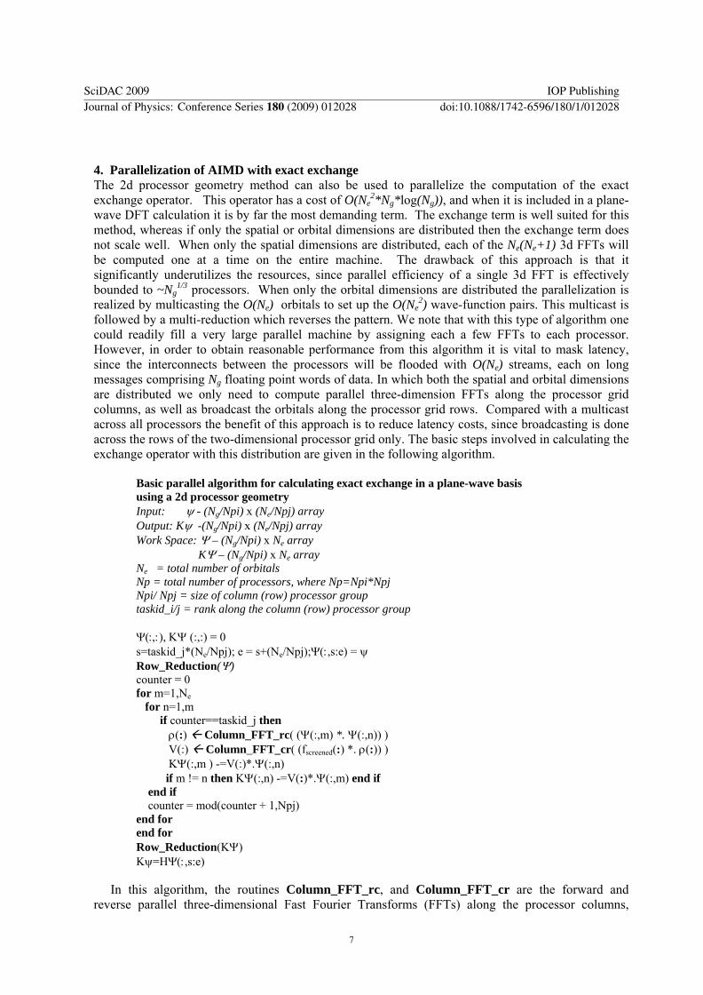