Santa Clara UniversityScholar Commons

Economics Leavey School of Business

12-2011

Happiness and Time Preference: The Effect ofPositive Affect in a Random-AssignmentExperimentJohn IfcherSanta Clara University, jifcher@scu.edu

Homa Zarghamee

Follow this and additional works at: http://scholarcommons.scu.edu/econ

Part of the Economics Commons

Copyright © 2011 by the American Economic Association.

This Article is brought to you for free and open access by the Leavey School of Business at Scholar Commons. It has been accepted for inclusion inEconomics by an authorized administrator of Scholar Commons. For more information, please contact rscroggin@scu.edu.

Recommended CitationIfcher, John, and Homa Zarghamee. 2011. "Happiness and Time Preference: The Effect of Positive Affect in a Random-AssignmentExperiment." American Economic Review, 101(7): 3109-29.

American Economic Review 101 (December 2011): 3109–3129http://www.aeaweb.org/articles.php?doi=10.1257/aer.101.7.3109

3109

Initially ignored, and subsequently thought to be disruptive, emotions have his-torically received a bum rap from decision researchers (George Loewenstein and Jennifer S. Lerner 2003; Alice M. Isen 2008). A great deal of recent research, how-ever, has shown that emotions can have important and, in the case of mild posi-tive affect, often salutary effects (Isen 2008). For example, positive affect has been shown to increase cognitive flexibility (Isen 2008); reciprocity in “gift-exchange” games (Georg Kirchsteiger, Luca Rigotti, and Aldo Rustichini 2006); work effort and productivity (Amir Erez and Isen 2005; Andrew Oswald, Eugenio Proto, and Daniel Sgroi 2008); loss aversion (Isen, Thomas E. Nygren, and Gregory F. Ashby1988); and risk aversion when the stakes are high (Isen and Nehemia Geva 1987). It has also been shown to decrease spending and willingness to pay (Lerner, Deborah A. Small, and Loewenstein 2004; Cynthia E. Cryder et al. 2008); and risk aversion when the stakes are low (Isen and Geva 1987). We conduct a random-assignment experiment to investigate whether positive affect impacts time prefer-ence, where time preference denotes a preference for present over future utility (Shane Frederick, Loewenstein, and Ted O’Donoghue 2002). Our results indicate that mild positive affect significantly reduces subjects’ time preference.

Because an individual’s rate of time preference affects his or her decisions, econo-mists have shown tremendous interest in modeling and estimating time preference

Happiness and Time Preference: The Effect of Positive Affect in a Random-Assignment Experiment†

By John Ifcher and Homa Zarghamee*

We conduct a random-assignment experiment to investigate whether positive affect impacts time preference, where time preference denotes a preference for present over future utility. Our result indicates that, compared to neutral affect, mild positive affect significantly reduces time preference over money. This result is robust to various specifica-tion checks, and alternative interpretations of the result are consid-ered. Our result has implications for the effect of happiness on time preference and the role of emotions in economic decision making, in general. Finally, we reconfirm the ubiquity of time preference and start to explore its determinants. (JEL D12, D83, I31)

* Ifcher: Department of Economics, Santa Clara University, 500 El Camino Real, Santa Clara, CA 95053 (e-mail: jifcher@scu.edu); Zarghamee: Department of Economics, Santa Clara University, Santa Clara, CA 95053 (e-mail: hzarghamee@scu.edu). We wish to thank Abigail Brown, Rachel Croson, Michael Kevane, Silvana Krasteva, Erin Krupka, Eugenio Proto, Tanya Rosenblat, William Schulze, William Sundstrom, Neslihan Uler, three anonymous referees, and seminar participants at various locations. We also wish to thank Marianne Farag and Anders Loven-Holt, who provided excellent research assistance. Financial support from Santa Clara University’s Presidential Research Grant DPROVO98 and Leavey Grant is gratefully acknowledged. The authors contributed equally to this work.

† To view additional materials, visit the article page at http://www.aeaweb.org/articles.php?doi=10.1257/aer.101.7.3109.

3110 THE AMERICAN ECONOMIC REVIEW DECEMBER 2011

(Richard H. Thaler and Hersh M. Shefrin 1981; Loewenstein and Drazen Prelec 1992; David Laibson 1997; Maribeth Coller and Melonie B. Williams 1999; O’Donoghue and Matthew Rabin 1999; Faruk Gul and Wolfgang Pesendorfer 2001; John T. Warner and Saul Pleeter 2001; Glenn W. Harrison, Morten I. Lau, and Williams 2002; Coller, Harrison, and E. Elisabet Rutstrom 2003; Ariel Rubinstein 2003; Jess Benhabib and Alberto Bisin 2005; Harrison and Lau 2005; Jesse M. Shapiro 2005; Steffen Andersen et al. 2008). Time preference has been shown to be commonplace, is believed to lead to self-control problems, and may increase the likelihood of negative outcomes—for example, overconsumption, obesity, addic-tion, reduced human capital accumulation, and diminished retirement saving (Kris N. Kirby, Nancy M. Petry, and Warren K. Bickel 1999; Frederick, Loewenstein, and O’Donoghue 2002; B. Douglas Bernheim and Antonio Rangel 2004; John Ameriks et al. 2007; Benhabib, Bisin, and Andrew Schotter 2010). Walter Mischel, Yuichi Shoda, and Monica L. Rodriguez (1989) found that preschoolers’ ability to delay gratification was a strong predictor of SAT scores over a decade later.

Initial empirical evidence for our result comes from the General Social Survey (GSS), which in three waves (1973, 1974, and 1976) includes both a measure of self-reported happiness (“Taken all together, how would you say things are these days—would you say that you are very happy, pretty happy, or not too happy?”) and time preference (agreement or disagreement with the statement, “Nowadays, a per-son has to live pretty much for today and let tomorrow take care of itself.”). We find that happier respondents are less likely to agree with the “live for today” statement than are less happy respondents. This holds even after controlling for covariates that have been shown to be related to happiness (see Appendix Table A1 for regression results). While this empirical evidence provides loose support for our result, it has a number of shortcomings. Most notably, the direction of causation cannot be identi-fied. Further, this measure of time preference is imperfect at best. While in this paper we will study the impact of mild positive affect—rather than happiness—on time preference, our methodology will address both of these shortcomings.1

To explore the relationship between mild positive affect and time preference, we run a random-assignment experiment in which subjects’ time preference is measured after their mood has been manipulated. Specifically, subjects are randomly assigned to the treatment group (positive affect) or the control group (neutral affect). The appropriate affect is induced using short video clips. Time preference is measured using a standard matching procedure, in which subjects report the present value of a future payment and truthful responses are incentivized.

Our results indicate that subjects in the treatment group exhibit significantly lower time preference than do subjects in the control group. This result is robust to vari-ous specification checks. The next section of this paper provides a brief overview of the literature; the third and fourth sections describe the experimental design and the econometric specifications, respectively; the fifth section presents the results; the sixth section discusses three alternative explanations for the result; finally, in the discussion section, potential mechanisms are discussed, along with implications of the result.

1 The degree to which one can generalize from our result to the impact of happiness on time preference is explored in the discussion section.

3111IFCHER AND zARgHAMEE: HAppINEss AND TIME pREFERENCEVOL. 101 NO. 7

I. Literature Review

The impact of mild positive affect on decision making has been extensively stud-ied over the past 20 years. Researchers, most notably Alice M. Isen, have conducted controlled experiments that demonstrate that mild positive affect can have beneficial effects on decision making, increasing cognitive flexibility, work effort, helpful-ness, and creativity (recent reviews include Sonja Lyubomirsky, Laura King, and Ed Diener 2005; Isen 2008). Moreover, mild positive affect does not appear to impede decision making as many would expect it to. For example, there is no experimental evidence that mild positive affect causes individuals to be impulsive, thoughtless, or overly optimistic (Isen 2007).

Research that explores the impact of positive affect on self-control is most rel-evant to our study, since the psychological concept of a lack of self-control overlaps with the economic concept of time preference. For example, Dianne M. Tice and Ellen Bratslavsky (2000) reported that psychologists generally understand a lack of self-control to be distinguished by a proclivity toward short-term gains, even in the face of long-term costs. Three recent psychological studies are of particu-lar interest: first, Roy E. Baumeister, Bratslavsky, and Tice (1998) found that mild positive (negative) affect increases (decreases) the proportion of time subjects spent studying for a nonincentivized test in the laboratory; second, Isen and Johnmarshall Reeve (2005) demonstrated that mild positive affect increases intrinsic motiva-tion for interesting tasks; and third, Isen (2007) reported that mild positive affect replenishes will power.2 These results are taken to indicate that mild positive affect increases forward-looking thinking, the ability to stay on task, and self-control. In summary, this line of research is far smaller and less well corroborated than other research regarding the impact of mild positive affect on decision making, leading Isen and Reeve (2005) to conclude that “the topic of the role of positive affect in development of self-control seems a promising one for investigation.”

A related strand of economic literature considers the effect of self-control on sub-jective well-being. This research attempts to identify the impact of poor self-control by comparing the happiness of individuals who make decisions that are thought to result from a lack of self-control to those who do not make such decisions. For example, Bruno S. Frey, Christine Benesch, and Alois Stutzer (2007) found that frequent TV watchers report being less happy; and Stutzer (2007) found that obe-sity reduces the subjective well-being of individuals who report having limited self-control. Further, Jonathan Gruber and Sendhil Mullainathan (2005) found that cigarette taxes increase happiness among individuals prone to smoke. The authors interpreted the tax as a self-control device, which suggests that a lack of self-control may cause unhappiness. These studies appear to indicate that a lack of self-control reduces happiness. By extension this suggests that time preference may affect posi-tive affect. While this direction of causation—the opposite of the one tested in this

2 Six more studies considering the effect of affect on self-control have been conducted exclusively with young children (Mischel, Brian Coates, and Antonette Raskoff 1968; Mischel, Ebbe B. Ebbesen, and Antonette Raskoff Zeiss 1973; Bill Underwood, Bert S. Moore, and D. L. Rosenhan 1973; Gloria Seeman and J. Conrad Schwarz 1974; P. S. Fry 1975; and Schwarz and Pamela R. Pollack 1977). For developmental reasons, the results of these papers cannot be generalized to adults (Alessandro Bucciol, Daniel Houser, and Marco Piovesan 2011).

3112 THE AMERICAN ECONOMIC REVIEW DECEMBER 2011

study—may hold, it is outside of the scope of the current paper to explore this possibility.3

Finally, this research adds to a small literature regarding the determinants of time preference. Two well-established results in this literature are that (i) the magnitude of the future payment, and (ii) the length of time over which discounting occurs, are important determinants of time preference (Thaler 1981; Kirby and Nino Marakovic 1996). More recently, it has been shown that (i) high cognitive load increases time preference (John M. Hinson, Tina L. Jameson, and Paul Whitney 2003; Daniel J. Benjamin, Sebastian A. Brown, and Shapiro 2006); and (ii) individuals with greater cognitive skills, as measured by IQ tests, exhibit lower time preference (Stephen V. Burks et al. 2009). This study adds to the literature by identifying a new determinant of time preference.

II. Experimental Design

We examined the effect of positive affect on time preference in a laboratory experiment conducted at Santa Clara University. In brief, the experimental proce-dure was as follows (additional details are provided below). First, subjects read and signed an informed-consent form. Second, subjects were instructed (i) that they would be answering 30 time-preference questions; (ii) that their payment would be based on one of these questions; (iii) that the payment question would be determined randomly at the end of the session; (iv) that a mechanism would be used to provide an incentive for truthful responses; and (v) that they would receive certificates of guarantee for their payments that could be redeemed for cash off-site after the experiment. Third, the mood-inducement procedure was administered. Fourth, subjects answered the 30 time-preference questions. Fifth, subjects answered questions regarding their subjective well-being and mood. Sixth, payments were determined. Seventh, subjects answered questions regarding their demographic and psychological characteristics. Finally, subjects received their certificates of guarantee, which included detailed redemption instructions. In total, the experiment lasted approximately 45 minutes, and subjects received an average of $24 for their participation.

A. participants

Sixty-nine undergraduate students were recruited from introductory English courses that all Santa Clara students are required to take; these courses were chosen in an attempt to avoid potential disciplinary bias.

B. participant Instructions

After completing the informed-consent form, subjects received detailed written instructions, which were also read aloud by the experimenter. The instructions

3 An additional paper, Eleanor H. Wertheim and Schwarz (1983), found that self-reported depression was cor-related with a preference for immediate (delayed) benefits (costs). This study is correlational and does not provide any evidence regarding a causal relationship in either direction.

3113IFCHER AND zARgHAMEE: HAppINEss AND TIME pREFERENCEVOL. 101 NO. 7

introduced the time-preference questions and informed the subjects that the experimental procedure had been designed to encourage truthful responses. Specifically, subjects were told that the 30 time-preference questions would be of the following form: “What amount of money, $p, if paid to you today would make you indifferent to $m paid to you in t days?” Five values of m, {$11.34, $18.31, $24.28, $32.84, $51.71}, and six values of t, {1 day, 3 days, 7 days, 14 days, 28 days, 56 days}, were used. We chose abstruse values for m to discourage the use of heuristics, such as answering one-half of m for each p. The questions were randomized so that there was no pattern in the order of the values of m or t; this was done to avoid anchoring. The time delay, t, was not extended beyond two months so that all possible payouts would occur within the academic term. Also, values of t were chosen to avoid weekends and school holidays and, with the exception of the one- and three-day delays, to fall on the same day of the week as the experimental session.

Subjects were informed that their payment would be based on one of the 30 time-preference questions, that the payment question would be determined ran-domly at the end of the session, and, thus, that they should answer each question as if their payment depended on it. Subjects were then introduced to the Becker-DeGroot-Marschak (BDM) mechanism and informed that it would be used to provide an incentive for truthfully answering the 30 time-preference questions (Gordon M. Becker, Morris H. Degroot, and Jacob Marschak 1964; Benhabib, Bisin, and Schotter 2010). Specifically, the amount and timing of the payment were determined as follows (using the BDM mechanism): m balls numbered 1 through m were placed in a spinner, and one was chosen. If the number R on the drawn ball was less than or equal to p, then the subject was paid $m in t days. If the number drawn exceeded p, the subject was paid $R on the day of the experimental session. Finally, note that since the values of m were fractional, the number of balls placed in the spinner was rounded to the next highest integer. For example, if m = $11.34, then balls numbered 1 through 12 were placed in the spinner. Finally, subjects were guided through numerous examples in an attempt to ensure that they understood the process.4

Subjects were also informed of the payment-pickup process, which was designed carefully in an attempt to equalize the transaction costs and uncertainty associated with experimental payments—challenging design issues in all time-preference experiments. For example, consider a design wherein present payments are distrib-uted on-site at the end of the experimental session, and future payments are distrib-uted off-site. Then the transaction costs associated with future payments are higher than those associated with present payments (since future payments require subjects to make an additional trip to retrieve their payment). Consequently, subjects’ prefer-ence for present versus future payments could be affected by this cost differential, confounding any measure of time preference.

In our experiment, subjects were issued certificates of guarantee at the end of the experimental session for all payments. These certificates were redeemable for

4 Subjects did not answer the 30 time-preference questions at this time. Rather, they answered them immediately following the mood-inducement procedure. This order of events eliminated the possibility that the induced mood could have been moderated, if not nullified, by reading the participant instructions.

3114 THE AMERICAN ECONOMIC REVIEW DECEMBER 2011

cash at an administrative office, which was in a different building than the one in which the experimental session was conducted (see Coller and Williams 1999; Harrison, Lau, and Williams 2002). The certificate also indicated the payment amount and the location where, and time after which, the certificate could be redeemed for cash. Even subjects receiving present (same-day) payments were required to wait one hour to redeem their certificates. Further, the certificate included contact information for the experimenters—professors at Santa Clara University—and instructed subjects to contact the experimenters if there were any problems redeeming their certificates (see James Andreoni and Charles Sprenger 2010a, b).

Subjects were also informed of the anonymous and blind nature of the payment process. They were told (i) that one person would prepare the payment envelopes; (ii) that a second person would distribute the sealed payment envelopes; (iii) that neither would know the subject’s identity, only the subject identification number; and (iv) that the envelope-distributor would not know the payment amount. This procedure was implemented in an attempt to minimize the potentially confounding role of subject-experimenter reciprocity.

C. Mood-Inducement procedure

We attempted to manipulate subjects’ mood by showing them a short film clip. The use of film clips to induce moods is common in psychological and, increasingly, economic experiments (James J. Gross and Robert W. Levenson 1995; Kirchsteiger, Rigotti, and Rustichini 2006; Jonathan Rottenberg, Rebecca D. Ray, and Gross 2007; Oswald, Proto, and Sgroi 2008). Rainer Westerman et al. (1996) evaluated eleven mood-inducement procedures. They found that the use of film or story was the most effective means of inducing positive affect.

In our experiment, half of the subjects (34 of 69) were randomly assigned to the treatment group and watched a film clip intended to induce positive affect. The other half of the subjects (35 of 69) were assigned to the control group and watched a film clip intended to induce neutral affect. Except for the variant film clip, the experi-mental protocol was identical for the control and treatment groups.

Our choice of film clips followed Gross and Levenson (1995). There, over 200 film clips were evaluated for their efficacy in inducing each of 7 different affects. Nearly 500 subjects were asked to rate on a scale from 0 to 8 the greatest intensity of each affect they felt during the course of the film clip. The strongest affect felt during the clip was dubbed the target affect for that film. The authors then reported the two most effective clips for inducing each of the affects.

In our experiment, the positive-affect film clip was a short montage of stand-up comedy bits from the 2002 Robin Williams: Live on Broadway. This choice fol-lowed directly from Gross and Levenson (1995), in which one of the two most successful positive-affect-inducing film clips was Robin Williams’s 1986 A Night at the Met. We opted for the 2002 montage primarily because it was more current and reduced concerns of the humor being outdated. The neutral-affect film clip was also one commonly used by psychologists and featured tranquil images of landscapes and wildlife in Denali National Park, Alaska (for example, Rottenberg, Ray, and Gross 2007).

3115IFCHER AND zARgHAMEE: HAppINEss AND TIME pREFERENCEVOL. 101 NO. 7

The success of the mood-inducement procedure was measured using the Positive and Negative Affect Schedule (PANAS), which was administered immediately after the time-preference questions. The PANAS asks subjects to rate on a scale from 1 to 10 how much of each of 7 positive and 9 negative affects they feel. The positive affects are amusement, arousal, contentment, happiness, interest, relief, and sur-prise; the negative affects are anger, confusion, contempt, disgust, embarrassment, fear, pain, sadness, and tension. In addition, subjects were asked whether the film clip made them happier, sadder, or neither; and whether the film clip put them in a better mood, worse mood, or neither.

D. Time-preference Questions and Completing the session

Immediately following the mood-inducement procedure, subjects answered the 30 time-preference questions. Then, subjects answered questions about their subjective well-being. Next, the payment question was determined, and the BDM mechanism was implemented. Finally, subjects answered questions regarding their demographic and psychological characteristics, including happiness and personal-ity traits.

The measure of happiness comes from the question, “Taken all together, how would you say things are these days—would you say that you are … ,” where possible responses ranged from 1 (completely unhappy) to 7 (completely happy). This measure is similar to the ones used in the GSS and the World Values Survey (WVS), each of which has been used extensively in the happi-ness-economics literature as a measure of long-term happiness. The GSS, how-ever, uses a three-point scale and the WVS a four-point scale. We expanded the scale to seven points to increase sensitivity. This question was asked after the mood-inducement procedure and the time-preference questions, but because of its broad scope, it should not have been affected by the treatment (Daniel Kahneman, Diener, and Norbert Schwarz 1999).

When all surveys were completed, subjects received certificates of guarantee for their payments and exited the experimental session.

III. Econometric Specifications

In analyzing the relationship between positive affect and time preference, we con-sider a model of the form

(1) p = βH + ∑ m

δ m I M (m) + ∑ t

α t I T (t)

+ ∑ m

∑ t

ϕ mt I M (m) × I T (t) + ∑ K

∑ k

λ Kk I K (k) + ε,

where H is a dummy for the positive-affect treatment, M is the set of all future pay-ment amounts m, T is the set of all time delays t (in days), and p is the subjective present value of $m in t days. The indicator functions IM(m) and IT(t) take the value of one for a given m and t, respectively, and zero otherwise; this specification allows for all possible linear and interacted effects of time delay and future payments on

3116 THE AMERICAN ECONOMIC REVIEW DECEMBER 2011

discounting. The model also includes demographic controls. The set of controls is denoted by K, and for a given control, k is the set of possible values. For example, for K = gender, k ∈ {male, female}, and Igender(male) equals one if the subject is male, and zero otherwise.

In this specification, the amount $p necessary today to be indifferent to $m in t days is considered to be a function of m, t, and m × t; that is, the regression is fully saturated with respect to the effect of time and future payments on present value. The appeal of this econometric specification is that it imposes minimal ex ante struc-ture and does not depend on the distribution of p. Thus, this parametrization does not restrict us to a specific model of discounting and fits the conditional expectation function for p perfectly (Joshua D. Angrist and Jorn-Steffen Pischke 2009).

Our choice of the fully saturated model follows from the underwhelming support we found for the exponential, fixed-cost, and hyperbolic models of discounting, which we estimated and tested using the techniques described in Benhabib, Bisin, and Schotter (2010).5 Those authors also rejected the exponential and hyperbolic models, though they found support for fixed-cost discounting.

Finally, OLS is used to estimate equation (1). Corrected standard errors are calcu-lated by clustering observations by subject; this is necessary since subjects answered 30 questions and their responses are unlikely to be independent.

IV. Results

A. Demographic Characteristics of subjects

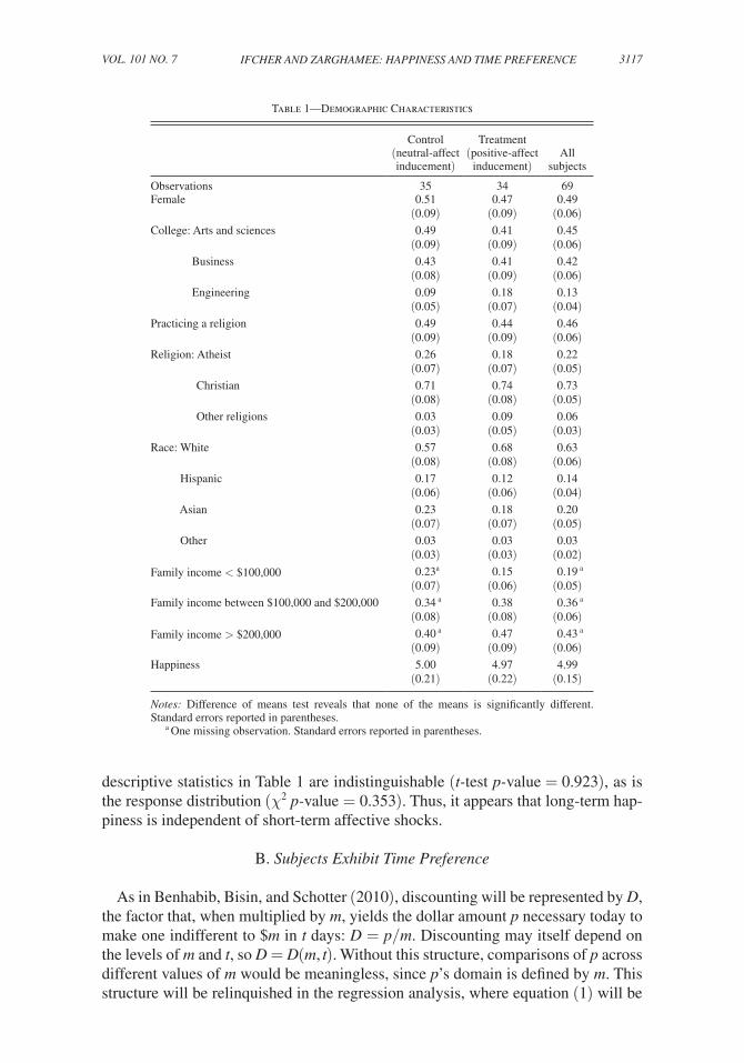
There is no significant difference between the values of any of the demographic characteristics for the treatment and control groups, so random assignment is valid ex post (see Table 1). Approximately half of the subjects are female. The division of students across colleges roughly mimics the university’s population. Santa Clara University has three colleges: arts and sciences, business, and engineering. Only a small number of subjects are in the engineering college; the rest are evenly split between arts and sciences and business. Roughly half of the subjects report that they practice a religion. Given that Santa Clara is a Jesuit university, it is not surprising that the most heavily represented religion is Christianity, accounting for three-quar-ters of the subjects. Almost all other subjects consider themselves atheists, with only two students identifying a different religion. The next demographic factor we con-trol for is race. Almost all of the subjects consider themselves white (63 percent), Asian (20 percent), or Hispanic (14 percent), with only two subjects identifying with other racial/ethnic categories. Finally, subjects were asked to give their best estimate of their family income. The mean response falls in the $100,000–$150,000 category, while the median is in $150,000–$200,000 category. Few students report family income of less than $80,000 or greater than $500,000.

As noted above, the measure of long-term happiness is hypothesized to be unaffected by mood inducement. Indeed, there is no statistical difference in hap-piness for the treatment and control groups. Mean responses, reported with other

5 Please contact the authors for complete results.

3117IFCHER AND zARgHAMEE: HAppINEss AND TIME pREFERENCEVOL. 101 NO. 7

descriptive statistics in Table 1 are indistinguishable (t-test p-value = 0.923), as is the response distribution (χ2 p-value = 0.353). Thus, it appears that long-term hap-piness is independent of short-term affective shocks.

B. subjects Exhibit Time preference

As in Benhabib, Bisin, and Schotter (2010), discounting will be represented by D, the factor that, when multiplied by m, yields the dollar amount p necessary today to make one indifferent to $m in t days: D = p/m. Discounting may itself depend on the levels of m and t, so D = D(m, t). Without this structure, comparisons of p across different values of m would be meaningless, since p’s domain is defined by m. This structure will be relinquished in the regression analysis, where equation (1) will be

Table 1—Demographic Characteristics

Control (neutral-affect inducement)

Treatment (positive-affect

inducement)All

subjects

Observations 35 34 69Female 0.51 0.47 0.49

(0.09) (0.09) (0.06)College: Arts and sciences 0.49 0.41 0.45

(0.09) (0.09) (0.06) Business 0.43 0.41 0.42

(0.08) (0.09) (0.06) Engineering 0.09 0.18 0.13

(0.05) (0.07) (0.04)Practicing a religion 0.49 0.44 0.46

(0.09) (0.09) (0.06)Religion: Atheist 0.26 0.18 0.22

(0.07) (0.07) (0.05) Christian 0.71 0.74 0.73

(0.08) (0.08) (0.05) Other religions 0.03 0.09 0.06

(0.03) (0.05) (0.03)Race: White 0.57 0.68 0.63

(0.08) (0.08) (0.06) Hispanic 0.17 0.12 0.14

(0.06) (0.06) (0.04) Asian 0.23 0.18 0.20

(0.07) (0.07) (0.05) Other 0.03 0.03 0.03

(0.03) (0.03) (0.02)Family income < $100,000 0.23a 0.15 0.19 a

(0.07) (0.06) (0.05)Family income between $100,000 and $200,000 0.34 a 0.38 0.36 a

(0.08) (0.08) (0.06)Family income > $200,000 0.40 a 0.47 0.43 a

(0.09) (0.09) (0.06)Happiness 5.00 4.97 4.99

(0.21) (0.22) (0.15)

Notes: Difference of means test reveals that none of the means is significantly different. Standard errors reported in parentheses.

a One missing observation. Standard errors reported in parentheses.

3118 THE AMERICAN ECONOMIC REVIEW DECEMBER 2011

estimated using the absolute level of p as the dependent variable. Table 2 presents observed values of D for all (m, t)-combinations; Table 2A pools all subjects, and Tables 2B and 2C present the treatment and control groups, respectively.

Subjects consistently discount the distant future more heavily than they do the near future. Holding m constant, D clearly trends downward in all panels of Table 2; this is visualized in Figure 1A for the pooled data. In Tables 2A and 2C, there are few exceptions to the downward trend. The monotonicity of the negative relation-ship between D and t is violated more frequently in the positive-affect treatment (see Table 2B), but in general the relationship holds.

The relationship between future payment m and the discount factor D, holding t constant, does not follow so consistent a pattern. For virtually no time delay t is

Table 2A– D(m, t), Pooled Data, 69 Subjects

t(Days)m(Dollars) 1 3 7 14 28 56 Mean

$11.34 0.910 0.890 0.846 0.814 0.795 0.766a 0.837a

(0.215) (0.171) (0.203) (0.210) (0.238) (0.260) (0.223)$18.31 0.928 0.889 0.856 0.833 0.786 0.752 0.841

(0.200) (0.195) (0.217) (0.207) (0.235) (0.272) (0.229)$24.28 0.910b 0.893 0.853 0.838 0.847 0.757 0.849b

(0.221) (0.201) (0.227) (0.209) (0.169) (0.253) (0.219)$32.84 0.915 0.898 0.851 0.857a 0.775 0.778 0.846a

(0.211) (0.177) (0.219) (0.160) (0.252) (0.244) (0.219)$51.71 0.931 0.882 0.889 0.840 0.823 0.779 0.857

(0.212) (0.241) (0.248) (0.258) (0.246) (0.265) (0.249)Mean 0.919b 0.890 0.859 0.836a 0.805 0.766a 0.846c

(0.211) (0.197) (0.222) (0.211) (0.230) (0.258) (0.228)

Note: Standard errors reported in parentheses.a One missing response.b Three missing responses.c Five missing responses.

Table 2B– D(m, t), Treatment Group, 34 Subjects

t(Days)m(Dollars) 1 3 7 14 28 56 Mean

$11.34 0.941 0.909 0.874 0.837 0.841 0.806 0.868(0.167) (0.123) (0.159) (0.214) (0.198) (0.246) (0.192)

$18.31 0.947 0.906 0.910 0.875 0.813 0.786 0.873(0.157) (0.184) (0.131) (0.149) (0.232) (0.258) (0.197)

$24.28 0.968b 0.936 0.892 0.901 0.895 0.832 0.903b

(0.071) (0.115) (0.160) (0.114) (0.131) (0.203) (0.143)$32.84 0.933 0.928 0.889 0.889a 0.813 0.839 0.882a

(0.173) (0.107) (0.159) (0.129) (0.224) (0.213) (0.176)$51.71 0.963 0.903 0.964 0.871 0.851 0.840 0.899

(0.171) (0.211) (0.053) (0.209) (0.231) (0.222) (0.197)Mean 0.950b 0.917 0.906 0.875a 0.843 0.821 0.885c

(0.152) (0.153) (0.141) (0.168) (0.206) (0.228) (0.182)

Note: Standard errors reported in parentheses.a One missing response.b Two missing responses.c Three missing responses.

3119IFCHER AND zARgHAMEE: HAppINEss AND TIME pREFERENCEVOL. 101 NO. 7

there monotonicity in D with respect to m. Nor is there a clear nonmonotonic trend (for example, in Table 2A, for t = 1, D has two interior peaks; for t = 14, there appears to be an inverted U-shape; and for t = 56, a U-shape).

C. Mood Inducement Is successful

Mood inducement had the intended effect on affect. The net positive affect—the sum of the positive affects minus the sum of negative affects from the PANAS—of subjects in the positive-affect treatment was significantly higher than that of

Table 2C–D(m, t), Control Group, 35 Subjects

t(Days)

m(Dollars) 1 3 7 14 28 56 Mean

$11.34 0.880 0.871 0.819 0.792 0.751 0.725a 0.807a

(0.252) (0.208) (0.237) (0.208) (0.268) (0.356) (0.246)$18.31 0.909 0.873 0.803 0.792 0.760 0.719 0.809

(0.235) (0.206) (0.268) (0.246) (0.239) (0.284) (0.253)$24.28 0.856a 0.852 0.816 0.777 0.800 0.684 0.798a

(0.292) (0.253) (0.274) (0.258) (0.190) (0.277) (0.263)$32.84 0.897 0.869 0.815 0.828 0.738 0.718 0.811

(0.243) (0.223) (0.261) (0.182) (0.274) (0.259) (0.248)$51.71 0.897 0.861 0.816 0.810 0.795 0.720 0.817

(0.243) (0.268) (0.330) (0.299) (0.260) (0.293) (0.286)Mean 0.889a 0.865 0.814 0.800 0.769 0.713a 0.808b

(0.251) (0.230) (0.272) (0.240) (0.246) (0.274) (0.259)

Note: Standard errors reported in parentheses.a One missing response.b Two missing responses.

Table 2D–{DTreatment(m, t) − DControl(m, t)}, 34 Subjects in Treatment Group, 35 Subjects in Control Group

t(Days)m(Dollars) 1 3 7 14 28 56 Mean

$11.34 0.061 0.039 0.055 0.045 0.091 0.080a 0.055(0.052) (0.041) (0.049) (0.051) (0.057) (0.063) (0.037)

$18.31 0.038 0.034 0.107** 0.082* 0.053 0.067 0.063(0.048) (0.047) (0.051) (0.049) (0.057) (0.065) (0.041)

$24.28 0.111**a,b 0.083* 0.076 0.125** 0.094** 0.149** 0.111***(0.051) (0.048) (0.054) (0.048) (0.039) (0.059) (0.039)

$32.84 0.036 0.059 0.074 0.060b 0.074 0.122** 0.072*(0.051) (0.042) (0.052) (0.038) (0.060) (0.057) (0.040)

$51.71 0.064 0.043 0.149** 0.061 0.055 0.120* 0.082(0.051) (0.058) (0.057) (0.062) (0.059) (0.063) (0.050)

Mean 0.065 0.051 0.092** 0.076* 0.073 0.099* 0.081**(0.046) (0.042) (0.046) (0.041) (0.046) (0.052) (0.039)

Note: Standard errors reported in parentheses.*** Significant at the 1 percent level. ** Significant at the 5 percent level. * Significant at the 10 percent level.a One missing observation in control group.b Two missing observations in treatment group.

3120 THE AMERICAN ECONOMIC REVIEW DECEMBER 2011

subjects in the neutral-affect treatment (7.364 versus 0.531, p-value = 0.048 for one-sided t-test). Further, controlling for payment, watching the positive-affect clip made subjects significantly more likely to state that the film clip made them happier (p-value = 0.048) and put them in a better mood (p-value = 0.076).6

D. positive Affect Reduces Time preference

Preliminary support for positive affect reducing time preference can be seen in Table 2D, which reports the difference between DTreatment (m, t) and DControl (m, t). This difference is positive for each (m, t) combination; the positive-affect inducement

6 The last two affect checks are in the final questionnaire, which was administered after the payments were deter-mined; hence, the efficacy of mood inducement is tested, not with simple t-tests, but with regressions controlling for payment.

0.7

0.75

0.8

0.85

0.9

0.95

1

0 10 20 30 40 50 60t(Days)

D(m

, t)

$11.34 $18.31 $24.28 $32.84 $51.71

0.7

0.75

0.8

0.85

0.9

0.95

1

0 10 20 30 40 50 60

D(m

, t)

t(Days)

Panel B. D(m, t), averaging over m, by treatment, where avg = average, tr = treatment, and c = control

Panel A. D(m, t), holding m constant, pooled data

avg (treatment) $11.34 (tr) $18.31 (tr)

$24.28 (tr) $32.84 (tr) $51.71 (tr)

avg (control) $11.34 (c) $18.31 (c)

$24.28 (c) $32.84 (c) $51.71 (c)

Figure 1

3121IFCHER AND zARgHAMEE: HAppINEss AND TIME pREFERENCEVOL. 101 NO. 7

unambiguously reduces time preference. This is visualized in Figure 1, panel B, which separately illustrates the discount factors for the control and treatment groups over time delay t; the average discount factor for each group is emphasized.

Estimating equation (1) without demographic controls, we see further evidence that positive affect reduces time preference. Controlling for future payment amount and time delay, watching a positive- instead of neutral-affect film clip increases the present value of future payments by $2.20 on average (see column 1 of Table 3). This result is marginally statistically significant, with a p-value = 0.054. Further, the magnitude is quite substantial. Even for the largest value of m, $51.71, the increase in the present value of the future payment is over 4 percent. Since we are not study-ing the effects of time and monetary sums on time preference, the coefficients of the m and t dummies and their interactions are not presented.

In column 2, controls are added for gender, race, family income, religion, regular religious service attendance, and college. Treatment is now statistically significant, increasing present value by $2.01 on average. In columns 3 and 4, the analyses of columns 1 and 2, respectively, are repeated controlling for self-reported, long-term happiness. The main effect is stable regardless of the specification; thus, the results appear to be robust.7 Finally, we estimate equation (1) conditional on p < m; that is, we exclude observations in which subjects did not discount. With the restricted sam-ple, the magnitude and the significance of the treatment effect increase (see columns 5 through 8 of Table 3). The positive-affect inducement now increases the present value of a future payment by an average of $3.00 in each of the four restricted specifications.

7 These results are robust to inclusion of the summed responses to the statements regarding personality traits, for which there was no statistically significant difference by treatment.

Table 3—Results of Estimating Equation (1) (Dependent variable is present value, p)

(1) (2) (3) (4) (5) (6) (7) (8)

Treatment 2.202* 2.012** 2.337** 2.416** 2.997** 3.027** 3.028** 3.507***(1.124) (0.958) (1.100) (1.002) (1.352) (1.159) (1.265) (1.207)

Only discounter included — — — — Yes Yes Yes YesCollege — Yes — Yes — Yes — YesGender — Yes — Yes — Yes — YesRace — Yes — Yes — Yes — YesReligion — Yes — Yes — Yes — YesPracticing — Yes — Yes — Yes — YesIncome — Yes — Yes — Yes — YesSelf-reported happiness — — Yes Yes — — Yes YesExcludes observations, where p = m

— — — — Yes Yes Yes Yes

R2 0.748 0.794 0.751 0.795 0.680 0.744 0.683 0.745

Observations 2,065 2,035 2,065 2,035 1,471 1,447 1,471 1,447Clusters 69 68 69 68 58 57 58 57

Notes: Robust standard errors reported in parentheses. For five observations, the reported value of p was unintelli-gible and thus excluded from all specifications. Columns 2, 4, 6, and 8 have one fewer cluster, and up to 30 fewer observations, than columns 1, 3, 5, and 7, respectively, because one subject had unreported demographic character-istics. Columns 5–8 exclude observations where p = m. Ten subjects had p = m for all observations; thus there are ten fewer clusters in 5–8 than in 1–4.

*** Significant at the 1 percent level. ** Significant at the 5 percent level. * Significant at the 10 percent level.

3122 THE AMERICAN ECONOMIC REVIEW DECEMBER 2011

In summary, our experiment demonstrates that mild positive affect significantly increases the present value of a future payment, a result that is robust to a number of econometric-specification checks. The magnitude of the increase depends on the value of the future payment and the specification, ranging from 4 percent of the future pay-ment (specification 2, m = $51.71) to 30 percent (specification 8, m = $11.34).

V. Alternative Explanations

We interpret the increase in the present value of a future payment for subjects in the positive-affect treatment, relative to those in the neutral-affect treatment, to indi-cate that positive affect increases the discount factor. There are at least three other interpretations of our finding: (i) that the timing of the payment affects the perceived probability of receiving the payment; (ii) that affect influences risk preferences; and (iii) that positive affect substitutes for money.

To diminish the possibility that (i) could drive our result, we attempted to equalize the transaction costs and uncertainties associated with being paid today versus being paid in the future. As was discussed in the Experimental Design section, all subjects had to redeem their certificates of guarantee off-site, and present payments were not available until one hour after the experimental session ended; the experimenters took care—in the detailed verbal instructions at the beginning and end of the experi-mental session and in the instructions on the certificate of guarantee—to point out the consistency of the payment pickup process across present and future payments. An additional concern is that subjects may prefer present payments, as they may not be on campus on future payment dates. We do not believe that this concern is rel-evant, since all subjects were recruited from required classes that met at least twice a week in the same academic quarter as all experimental sessions and all potential (future) payment dates. Further, four of six future payment dates were on the same day of the week as the experimental session (exceptions are t = 1 day and 3 days, the discount factors of which do not appear biased, as can be seen in Figure 1, panel A). Finally, we do not believe that trust differentially affected transaction costs. We believe that subjects trusted us, as professors, and believed that we would honor the certificates of guarantee. Subjects were not offered extra credit or any incentive, other than the experimental payments, to participate; hence, their presence alone would appear to demonstrate a high level of trust.

Alternate explanation (ii) is that the present value of a future payment increases for subjects in the positive-affect treatment because positive affect influences risk preferences. In particular, our result is confounded if positive affect reduces either the perceived uncertainty or subjects’ risk aversion associated with receiving a future payment relative to a present payment. Alternate explanation (iii) is that posi-tive affect acts as a substitute for money today, making subjects in the positive-affect treatment more willing to postpone income to a state in which they may be in less of a good mood. We cannot refute (ii) and (iii) using our data, but we hope our paper stimulates future research that can better explain our central finding.8

8 An earlier, unpublished version of this paper argues that our proposed interpretation is more plausible than are (ii) and (iii); that paper is available on the AER website.

3123IFCHER AND zARgHAMEE: HAppINEss AND TIME pREFERENCEVOL. 101 NO. 7

VI. Discussion

Our research indicates that mild positive affect significantly reduces time prefer-ence. Since this result is derived from a random-assignment experiment, the rela-tionship between positive affect and time preference is presumably causal, with positive affect reducing time preference. Below, we discuss, in turn, mechanisms that may explain this relationship and its implications.

A. potential Mechanisms

The psychological literature, where the bulk of affect research has been reported, discusses two potential mechanisms that may explain why mild posi-tive affect decreases time preference. First, Isen (2008) states that mild positive affect increases cognitive flexibility by broadening focus and attention, promot-ing openness to information, and enabling improved integration of information. Thus, the observed reduction in time preference may result from a more thorough consideration of broader (including future) net benefits. In addition, support for this mechanism comes from what the psychological literature dubs the “dopamine hypothesis”: that the release of dopamine (the neurotransmitter linked to rewards) in areas of the brain responsible for cognitive flexibility is the mediating fac-tor in the effect of positive affect on behavior (F. Gregory Ashby, Isen, and And U. Turken 1999; Isen 2008). Second, the replenishment of will power may help explain our result. As mentioned in the literature review, mild positive affect has been shown to replenish will power (Isen 2007). Consequently, postinducement, subjects in the positive-affect treatment should have their will power replenished and, thus, exhibit greater patience for a future payment.

B. Implications

In this section, we discuss what can and cannot be extrapolated from our result and then turn to policy implications. To understand what can be extrapolated, it is impor-tant to recognize that the effects of affect do not lie on a continuum from intense positive affect to intense negative affect. In particular, the “continuum” is violated in three significant ways. First, the effect of intense positive affect is not necessar-ily an amplification of the effect of mild positive affect (Isen 2007). Thus, we can-not assume that intense positive affect would result in a further reduction of time preference. Second, negative affect does not necessarily have the opposite effect of positive affect. The independence of positive and negative affect is well established in psychology (Norman M. Bradburn 1969; Diener and Robert A. Emmons 1984; David Watson, Lee Anna Clark, and Auke Tellegen 1988; Lyubomirsky, King, and Diener 2005; Isen 2007). Moreover, neural research suggests the two are unrelated. Each is associated with a distinct neurotransmitter: dopamine with positive affect and serotonin with negative affect. In other words, it should not be inferred from our result that negative affect would necessarily increase time preference. Third, two affects may have variant effects, even if both are positive or negative. For example, anger and sadness, while both negative affects, may have different effects on deci-sion making. In general, negative affects are more likely to have variant effects, and

3124 THE AMERICAN ECONOMIC REVIEW DECEMBER 2011

positive affects are less likely to have variant effects (Isen 2007).9 Thus, our result may not be specific to the particular positive affect induced—amusement—and may apply to a wide range of positive affects.

We now turn to the relationship between positive affect and happiness, that is, the relationship between being in a happy mood and being happy. In our experiment, we successfully improved subjects’ mood, but were unable—not surprisingly—to change subjects’ underlying, long-term happiness.  Thus, can we validly claim that happier individuals should exhibit lower time preference?

The distinction between positive affect and happiness, and what this distinction means for studying the impact of happiness, have been considered by Lyubomirsky, King, and Diener (2005) and James Konow and Joseph Earley (2008). In the former, four possible strategies for identifying the impact of happiness are discussed. The least valid is a correlational study, due to the inherent difficulty of demonstrating causation.

Conversely, the ideal would be a random-assignment experiment, in which underly-ing happiness is manipulated. Such an experiment, however, is neither feasible nor ethical.  Hence, Lyubomirsky, King, and Diener (2005) argue that the best feasible approach is a random-assignment experiment in which positive affect is induced.  They argue that such an approach is a valid way to identify the impact of being happy since happier individuals experience more frequent positive affect (Diener and Martin E. P. Seligman 2004; Lyubomirsky, King, and Diener 2005). In fact, Diener, Ed Sandvik, and William Pavot (1991) state that “Frequent positive affect is both necessary and suffi-cient to produce the state we call happiness, whereas intense positive experience is not.” Thus, our result suggests that happier individuals should exhibit less time preference.

Regardless of how affect and happiness are related, our result on the impact of affect alone has important implications. Affective shocks are ubiquitous; it is easy to for-get how much we are subject to them. For example, quotidian experiences—a kind word from a loved one or the tedium of traffic—are often enough to perturb one’s affective state. While research on laboratory mood-inducement procedures suggests that the moods induced in our experiment would likely last approximately 15 minutes, affective shocks outside of the lab may last longer—for hours or even days.10 Indeed, outside of the lab, mood generated by weather has been shown to influence stock returns (Edward M. Saunders, Jr. 1993; David Hirshleifer and Tyler Shumway 2003); and affective changes due to sports outcomes have been linked to changes in political views, self-confidence, optimism, health, stock returns, and crime and suicide rates (see Alex Edmans, Diego Garcia, and Oyvind Norli 2007). That the behavioral differentials observed in our experiment were the result of a mild and short-lived affective shock underscores—and does not detract from—the potency of mood’s effect on behavior.

Mood is not the first domain in which seemingly trivial perturbations significantly affect behavior. Brigitte C. Madrian and Dennis F. Shea (2001) famously showed that if 401(k) has to be opted out of instead of into, both participation and savings rates dramatically increase. That research suggests that important decisions are not

9 We are considering the effect of negative affects on time preference in a separate paper, specifically focusing on the effects of sadness, anger, and fear. Of these treatments, we have already conducted the sadness treatment and are now turning to the others.

10 Isen, Margaret Clark, and Mark F. Schwartz (1976) and Isen and Joyce M. Gorgoglione (1983) estimate that the positive affect induced by a free gift, or by reading statements with a positive valence, lasts between 10 and 20 minutes. Further, Isen and Gorgoglione (1983) state that positive affect induced by film may last longer.

3125IFCHER AND zARgHAMEE: HAppINEss AND TIME pREFERENCEVOL. 101 NO. 7

necessarily insulated from seemingly inconsequential perturbations of the decision-making context. Further, it has been shown that once employees make their 401(k) decisions, they generally do not change them. An important implication discussed in that research is that defaults are critical and should be designed optimally; in other words, policymakers should strive to “get the default right” (Madrian and Shea 2001). Analogously, policymakers may be able to increase well-being by accounting for mood in the design of decision-making environments. As noted above, sports out-comes have been shown to affect political views; hence, scheduling elections closely following major national sports events may be distortionary. Our result would sug-gest that a benevolent employer could help employees increase their pension plan contributions by having them complete the requisite paperwork after an enjoyable orientation session or other mood-elevating activity. This momentary decision, influ-enced by positive affect, would have long-lasting and important consequences. One can easily imagine other important decisions that could be similarly influenced.

Another practical implication of our result is that individuals may benefit from awareness that their mood affects their behavior. For example, a new employee may want to postpone pension plan contribution decisions until he or she is in a happy mood. The new employee may even want to proactively put him- or her-self into a good mood. Indeed, evidence from the positive psychology literature suggests that people can manipulate their own affect (C. R. Snyder and Shane J. Lopez 2005). It should be noted that these implications are speculative, as further research is required to determine whether: (i) awareness of the effect of mood inter-acts in any way with the direct effect itself; or (ii) self-induced positive affect has the same influence on time preference as a positive affective shock. For example, Loewenstein (1996) identifies a “hot-cold empathy gap,” namely that people tend to mispredict the impact of emotions on their behavior, especially when trying to assess the effect of an emotion other than the one they are currently experiencing. Awareness of how to objectively understand the consequences of one’s own emo-tions can hence benefit decision makers. In summary, the practical implications of our research are similar to those called upon in Laibson (2001) in reference to the effect of cues on consumption: “ … when consumers understand these mechanisms, consumers try to influence the sequence of cues they experience (e.g., recovering alcoholics avoid the smell or sight of alcohol). Cues serve as an important endog-enous variable, which firms, consumers, and governments try to control.”

Our research also has important theoretical implications. A host of process-oriented economic models speak directly to the impact of affective shocks on intertemporal deci-sions (Loewenstein 1996; Loewenstein, O’Donoghue, and Rabin 2003; Loewenstein and O’Donoghue 2004; Drew Fudenberg and David K. Levine 2006). In particular, our result reveals a gap in the way that economists have modeled the role of affect. The common theme of many relevant theoretical models is the conflict between the desire for immediate and delayed gratification (Adam Smith 1759; Thaler and Shefrin 1981; Eddie Dekel, Barton L. Lipman, and Rustichini 2001; Gul and Pesendorfer 2001; Bernheim and Rangel 2004; Gul and Pesendorfer 2004; Loewenstein and O’Donoghue 2004; Benhabib and Bisin 2005; Fudenberg and Levine 2006). These models often include “dual selves,” and behavior results from a struggle between the immediate (emotional and visceral) components of the self and the purposeful, long-term, goal-oriented components of the self. More specifically, these models predict

3126 THE AMERICAN ECONOMIC REVIEW DECEMBER 2011

that the immediate self, and the factors that motivate it, disrupt the more reasoned and deliberate goals of the long-term self. So, while dual self models might effectively capture the phenomenon of “blind rage,” or how anger might influence behavior, how positive affect fits into these models is less clear.11 The need for a more nuanced view of affect—one that, like the psychological explanations discussed above, captures the salutary effect of some affects—is supported by our research. Relatedly, our research indicates that positive affect may change fundamental preferences. Thus, it is impor-tant to incorporate the impact of positive affect into economic models.

Finally, an important implication for other experimental researchers is that affect should be neutralized at the beginning of time preference experiments. Indeed, uncontrolled affect may be partially responsible for the highly variant estimates of discount rates reported in the time preference literature (Frederick, Loewenstein, and O’Donoghue 2002).

In summary, our experiment adds to the mounting evidence that positive affect influences behavior in economically important ways. We can only speculate, how-ever, upon how this effect comes to be. In addition, this study adds to the behavioral economics literature by identifying a determinant of time preference.

Appendix

11 The same can be said for relevant economic models that do not rely on dual selves, for example, Laibson’s (2001) cue theory of consumption.

Table A1—Results from Regressing “Live for Today” on Self-Reported Happiness

Dependent variable: Live for today (1 = “agree” and 0 = “disagree”) (1) (2)

Happiness (3 = “very happy,” 2 = “pretty happy,” and 1 = “not too happy”) −0.048*** −0.042**

(0.012) (0.021)Age — −0.006

(0.006)Age squared — 0.000

(0.000)Attend religious services at least once per month — 0.010

(0.026)Female — 0.062**

(0.028)Income below median (< $15,000) — 0.073**

(0.035)Low education (< 11 years) — 0.216***

(0.032)Nonwhite — 0.123***

(0.045)Poor or fair health — 0.073**

(0.036)Observations 1,636 1,636

Note: Standard errors reported in parentheses.*** Significant at the 1 percent level. ** Significant at the 5 percent level. * Significant at the 10 percent level.

3127IFCHER AND zARgHAMEE: HAppINEss AND TIME pREFERENCEVOL. 101 NO. 7

REFERENCES

Ameriks, John, Andrew Caplin, John Leahy, and Tom Tyler. 2007. “Measuring Self-Control Prob-lems.” American Economic Review, 97(3): 966–72.

Andersen, Steffen, Glenn W. Harrison, Morten I. Lau, and E. Elisabet Rutstrom. 2008. “Eliciting Risk and Time Preferences.” Econometrica, 76(3): 583–618.

Andreoni, James, and Charles Sprenger. 2010a. “Risk Preferences Are Not Time Preferences: Dis-counted Expected Utility with a Disproportionate Preference for Certainty.” National Bureau of Economic Research Working Paper 16348.

Andreoni, James, and Charles Sprenger. 2010b. “Estimating Time Preferences from Convex Budgets.” National Bureau of Economic Research Working Paper 16347.

Angrist, Joshua D., and Jorn-Steffen Pischke. 2009. Mostly Harmless Econometrics: An Empiricist’s Companion. Princeton: Princeton University Press.

Ashby, F. Gregory, Alice M. Isen, and And U. Turken. 1999. “A Neuropsychological Theory of Positive Affect and its Influence on Cognition.” psychological Review, 106(3): 529–50.

Baumeister, Roy E., Ellen Bratslavsky, and Dianne M. Tice. 1998. “Procrastination and Affect Regu-lation.” Unpublished.

Becker, Gordon M., Morris H. Degroot, and Jacob Marschak. 1964. “Measuring Utility by a Single-Response Sequential Method.” Behavioral science, 9(3): 226–32.

Benhabib, Jess, and Alberto Bisin. 2005. “Modeling Internal Commitment Mechanisms and Self-Control: A Neuroeconomics Approach to Consumption-Saving Decisions.” games and Economic Behavior, 52(2): 460–92.

Benhabib, Jess, Alberto Bisin, and Andrew Schotter. 2010. “Present-bias, Quasi-Hyperbolic Discount-ing, and Fixed Costs.” games and Economic Behavior, 69: 205–23.

Benjamin, Daniel J., Sebastian A. Brown, and Jesse M. Shapiro. 2006. “Who is ‘Behavioral’? Cogni-tive Ability and Anomalous Preferences.” SSRN Working Paper 675264.

Bernheim, B. Douglas, and Antonio Rangel. 2004. “Addiction and Cue-Triggered Decision Processes.” American Economic Review, 94(5): 1558–90.

Bradburn, Norman M. 1969. The structure of psychological Well-Being. Chicago: Aldine Publishing Company.

Bucciol, Alessandro, Daniel Houser, and Marco Piovesan. 2011. “Temptation and Productivity: A Field Experiment with Children.” Journal of Economic Behavior and Organization, 78(1–2): 126–36.

Burks, Stephen V., Jeffrey P. Carpenter, Lorenz Goette, and Aldo Rustichini. 2009. “Cognitive Skills Affect Economic Preferences, Strategic Behavior, and Job Attachment.” proceedings of the National Academy of sciences,106(19): 7745–50.

Coller, Maribeth, Glenn W. Harrison, and E. Elisabet Rutstrom. 2003. “Are Discount Rates Constant? Reconciling Theory and Observation.” University of Central Florida. Department of Economics Working Paper 3-31.

Coller, Maribeth, and Melonie B. Williams. 1999. “Eliciting Individual Discount Rates.” Experimental Economics, 2(2): 107–27.

Croson, Rachel, and Uri Gneezy. 2009. “Gender Differences in Preferences.” Journal of Economic Lit-erature, 47(2): 448–74.

Cryder, Cynthia E., Jennifer S. Lerner, James J. Gross, and Ronald E. Dahl. 2008. “Misery is not Miserly: Sad and Self-Focused Individuals Spend More.” psychological science, 19(6): 525–30.

Davis, James Allen, and Tom W. Smith. 2007. General Social Surveys, 1972-2006 [machine readable data file]/Principal Investigator, James A. Davis; Director and Co-Principal Investigator, Tom W. Smith; Co-Principal Investigator, Peter V. Marsden; Sponsored by National Science Foundation. NORC ed. Chicago: National Opinion Research Center [producer]; Storrs, CT: The Roper Center for Public Opinion Research, University of Connecticut [distributor].

Dekel, Eddie, Barton L. Lipman, and Aldo Rustichini. 2001. “Representing Preferences with a Unique Subjective State Space.” Econometrica, 69(4): 891–934.

Diener, Ed, and Robert A. Emmons. 1984. “The Independence of Positive and Negative Affect.” Jour-nal of personality and social psychology, 47(5): 1105–17.

Diener, Ed, Ed Sandvik, and William Pavot. 1991. “Happiness Is the Frequency, Not the Intensity, of Positive Versus Negative Affect.” In subjective Well Being: An Interdisciplinary perspective, ed. Fritz Strack, Michael Argyle, and Norbert Schwarz, 119–40. Oxford: Pergamon Press.

Diener, Ed, and Martin E.P. Seligman. 2004. “Beyond Money: Toward an Economy of Well-Being.” psychological science in the public Interest, 5(1): 1–31.

Edmans, Alex, Diego Garcia, and Oyvind Norli. 2007. “Sports Sentiment and Stock Returns.” Journal of Finance, 62(4): 1967–98.

Erez, Amir, and Alice M. Isen. 2005. “The Influence of Positive Affect on the Components of Expec-tancy Motivation.” Journal of Applied psychology, 87(6): 1055–67.

3128 THE AMERICAN ECONOMIC REVIEW DECEMBER 2011

Frederick, Shane, George Loewenstein, and Ted O’Donoghue. 2002. “Time Discounting and Time Preference: A Critical Review.” Journal of Economic Literature, 40(2): 351–401.

Frey, Bruno S., Christine Benesch, and Alois Stutzer. 2007. “Does Watching TV Make Us Happy?” Journal of Economic psychology, 28(3): 283–313.

Fry, P.S. 1975. “Affect and Resistance to Temptation.” Developmental psychology, 11(4): 466–72.Fudenberg, Drew, and David K. Levine. 2006. “A Dual-Self Model of Impulse Control.” American

Economic Review, 96(5): 1449–76.Gross, James J., and Robert W. Levenson. 1995. “Emotion Elicitation Using Films.” Cognition and

Emotion, 9(1): 87–108.Gruber, Jonathan, and Sendhil Mullainathan. 2005. “Do Cigarette Taxes Make Smokers Happier?” B

E Journal of Economic Analysis and policy: Advances in Economic Analysis and policy, 5(1): 1–43.Gul, Faruk, and Wolfgang Pesendorfer. 2001. “Temptation and Self-Control.” Econometrica, 69(6):

1403–35.Gul, Faruk, and Wolfgang Pesendorfer. 2004. “Self-Control and the Theory of Consumption.” Econo-

metrica, 72(1): 119–58.Harrison, Glenn W., and Morten I. Lau. 2005. “Is the Evidence for Hyperbolic Discounting in Humans

Just an Experimental Artefact?” Behavioral and Brain sciences, 28(5): 657.Harrison, Glenn W., Morten I. Lau, and Melonie B. Williams. 2002. “Estimating Individual Discount

Rates in Denmark: A Field Experiment.” American Economic Review, 92(5): 1606–17.Hinson, John M., Tina L. Jameson, and Paul Whitney. 2003. “Impulsive decision making and working

memory.” Journal of Experimental psychology: Learning, Memory, and Cognition, 29(2): 298–306.Hirshleifer, David, and Tyler Shumway. 2003. “Good Day Sunshine: Stock Returns and the Weather.”

Journal of Finance, 58(3): 1009–32.Ifcher, John, and Homa Shaghaghi Zarghamee. 2011. “Happiness and Time Preference: The Effect of

Positive Affect in a Random-Assignment Experiment: Dataset.”American Economic Review. http://www.aeaweb.org/articles.php?doi=10.1257/aer.101.7.3109.

Isen, Alice M. 2008. “Some Ways in Which Positive Affect Influences Decision Making and Problem Solving.” In Handbook of Emotions, ed. Michael Lewis, Jeannette M. Haviland-Jones, and Lisa Feldman Barrett, 548–73. New York: The Guilford Press.

Isen, Alice M. 2007. “Positive Affect, Cognitive Flexibility, and Self-Control.” In persons in Context: Building a science of the Individual, ed. Yuichi Shoda, Daniel Cervone, and Geraldine Downey, 130–47. New York: The Guilford Press.

Isen, Alice M., Margaret Clark, and Mark F. Schwartz. 1976. “Duration of the Effect of Good Mood on Helping: Footprints on the Sands of Time.” Journal of personality and social psychology, 34(3): 385–93.

Isen, Alice M., and Nehemia Geva. 1987. “The Influence of Positive Affect on Acceptable Level of Risk: The Person with a Large Canoe has a Large Worry.” Organizational Behavior and Human Decision processes, 39(2): 145–54.

Isen, Alice M., and Joyce M. Gorgoglione. 1983. “Some Specific Effects of Four Affect-Induction Pro-cedures.” personality and social psychology Bulletin, 9(1): 136–43.

Isen, Alice M., Thomas E. Nygren, and Gregory F. Ashby. 1988. “Influence of Positive Affect on the Subjective Utility of Gains and Losses: It is just not Worth the Risk.” Journal of personality and social psychology, 55(5): 710–17.

Isen, Alice M., and Johnmarshall Reeve. 2005. “The Influence of Positive Affect on Intrinsic and Extrinsic Motivation: Facilitating Enjoyment of Play, Responsible Work Behavior, and Self-Con-trol.” Motivation and Emotion, 29(4): 295–323.

Kahneman, Daniel, Ed Diener, and Norbert Schwarz. 1999. Well-being: The Foundations of Hedonic psychology. New York: The Russel Sage Foundation.

Kirby, Kris N., and Nino Marakovic. 1996. “Delay-Discounting Probabilistic Rewards: Rates Decrease as Amounts Increase.” psychonomic Bulletin & Review, 3(1): 100–4.

Kirby, Kris N., Nancy M. Petry, and Warren K. Bickel. 1999. “Heroin Addicts Have Higher Discount Rates for Delayed Rewards Than Non-Drug-Using Controls.” Journal of Experimental psychology: general, 128(1): 78–87.

Kirchsteiger, Georg, Luca Rigotti, and Aldo Rustichini. 2006. “Your Morals Might Be Your Moods.” Journal of Economic Behavior and Organization, 59(2):155–72.

Konow, James, and Joseph Earley. 2008. “The Hedonistic Paradox: Is Homo Economicus Happier?” Journal of public Economics, 92(1-2):1–33.

Laibson, David. 1997. “Golden Eggs and Hyperbolic Discounting.” Quarterly Journal of Economics, 112(2): 443–77.

Laibson, David. 2001. “A Cue-Theory of Consumption.” Quarterly Journal of Economics, 116(1): 81–119.

3129IFCHER AND zARgHAMEE: HAppINEss AND TIME pREFERENCEVOL. 101 NO. 7

Lerner, Jennifer S., Deborah A. Small, and George Loewenstein. 2004. “Heart Strings and Purse Strings.” psychological Bulletin, 15(5): 337–341.

Loewenstein, George. 1996. “Out of Control: Visceral Influences on Behavior.” Organizational Behav-ior and Human Decision Making, 65(3): 272–92.

Loewenstein, George, and Jennifer S. Lerner. 2003. “The Role of Affect in Decision Making”. In Handbook of Affective sciences, ed. Richard J. Davidson, Klaus R. Scherer, and H. Hill Goldsmith, 619–42. New York: Oxford University Press.

Loewenstein, George, and Ted O’Donoghue. 2004. “Animal Spirits: Affective and Deliberative Processes in Economic Behavior.” Cornell University, Center for Analytic Economics Working Paper 04-14.

Loewenstein, George, Ted O’Donoghue, and Matthew Rabin. 2003. “Projection Bias in Predicting Future Utility.” Quarterly Journal of Economics, 118(4): 1209–48.

Loewenstein, George, and Drazen Prelec. 1992. “Anomalies in Intertemporal Choice: Evidence and an Interpretation.” Quarterly Journal of Economics, 107(2): 573–97.

Lyubomirsky, Sonja, Laura King, and Ed Diener. 2005. “The Benefits of Frequent Positive Affect: Does Happiness Lead to Success?” psychological Bulletin, 131(6): 803–55.

Madrian, Brigitte C., and Dennis F. Shea. 2001. “The Power of Suggestion: Inertia in 401(K) Partici-pation and Savings Behavior.” Quarterly Journal of Economics, 116(4): 1149–87.

Mischel, Walter, Brian Coates, and Antonette Raskoff. 1968. “Effects of Success and Failure on Self-Gratification.” Journal of personality and social psychology, 10(4): 381–90.

Mischel, Walter, Ebbe B. Ebbesen, and Antonette Raskoff Zeiss. 1973. “Selective Attention to the Self: Situational and Dispositional Determinants.” Journal of peronality and social psychology, 27(1): 129–42.

Mischel, Walter, Yuichi Shoda, and Monica L. Rodriguez. 1989. “Delay of Gratification in Children.” science, 244(4907): 933–8.

O’Donoghue, Ted, and Matthew Rabin. 1999. “Doing It Now or Later.” American Economic Review, 89(1): 103–24.

Oswald, Andrew, Eugenio Proto, and Daniel Sgroi. 2008. “Happiness and Productivity.” Unpublished.Rottenberg, Jonathan, Rebecca D. Ray, and James J. Gross. 2007. “Emotion Elicitation Using Films.”

In The Handbook of Emotion Elicitation and Assessment, ed. James A. Coan and John J. B. Allen, 9–28. London: Oxford University Press.

Rubinstein, Ariel. 2003. “”Economics and Psychology”? The Case of Hyperbolic Discounting.” Inter-national Economic Review, 44(4): 1207–16.

Saunders, Edward M., Jr. 1993. “Stock Prices and Wall Street Weather.” American Economic Review, 83(5): 1337–45.

Schwarz, J. Conrad, and Pamela R. Pollack.1977. “Affect and Delay of Gratification.” Journal of Research in personality,11(2): 147–64.

Seeman, Gloria, and J. Conrad Schwarz.1974. “Affective State and Preference for Immediate versus Delayed Reward.” Journal of Research in personality, 7(4): 384–94.

Shapiro, Jesse M. 2005. “Is There a Daily Discount Rate? Evidence from the Food Stamp Nutrition Cycle.” Journal of public Economics, 89(2-3): 303–25.

Smith, Adam.1759.The Theory of Moral sentiments. Cambridge: Cambridge University Press, 2002.Snyder, C. R., and Shane J. Lopez, ed. 2005. Handbook of positive psychology. Oxford: Oxford Uni-

versity Press.Stutzer, Alois. 2007. “Limited Self-Control, Obesity, and the Loss of Happiness.” IZA Discussion

Paper 2925.Thaler, Richard H. 1981. “Some Empirical Evidence on Dynamic Inconsistency.” Economic Letters,

8(3): 201–7.Tice, Dianne M, and Ellen Bratslavsky. 2000. “Giving in to Feel Good: The Place of Emotion Regula-

tion in the Context of General Self-Control.” psychological Inquiry, 11(3): 149–59.Underwood, Bill, Bert S. Moore, and D. L. Rosenhan. 1973. “Affect and Self-Gratification.” Develop-

mental psychology, 8(2): 209–14.Warner, John T., and Saul Pleeter. 2001. “The Personal Discount Rate: Evidence from Military Down-

sizing Programs.” American Economic Review, 91(1): 33–53.Watson, David, Lee Anna Clark, and Auke Tellegen.1988. “Development and Validation of Brief Mea-

sures of Positive and Negative Affect: The PANAS Scales.” Journal of personality and social psy-chology, 54(6): 1063–70.

Wertheim, Eleanor H., and Schwarz, J. Conrad. 1983. “Depression, Guilt, and Self-Management of Pleasant and Unpleasant Events.” Journal of personality and social psychology, 45(4): 884–9.

Westerman, Rainer, Kordelia Spies, Gunter Stahl, and Friedrich W. Hesse.1996. “Relative Effective-ness and Validity of Mood Induction Procedures.” European Journal of social psychology, 26(4): 557–80.