Hammer Testing Findings for Solid-State Lighting Luminaires · Hammer Testing Findings for...
48
Hammer Testing Findings for Solid-State Lighting Luminaires December 2013 Prepared for: Solid-State Lighting Program Building Technologies Office Office of Energy Efficiency and Renewable Energy U.S. Department of Energy Prepared by: RTI International
Transcript of Hammer Testing Findings for Solid-State Lighting Luminaires · Hammer Testing Findings for...
Hammer Testing Findings for Solid-State Lighting Luminaires
December 2013
Prepared for:
Solid-State Lighting ProgramBuilding Technologies OfficeOffice of Energy Efficiency and Renewable EnergyU.S. Department of Energy
Prepared by:
RTI International
DOE/EE-1030
_________________________________ RTI International is a trade name of Research Triangle Institute.
RTI Project Number 0213159.002
Hammer Testing Findings for Solid-State Lighting Luminaires
Report
December 2013
Prepared for
LED Systems Reliability Consortium and the U.S. Department of Energy
Prepared by
RTI International 3040 Cornwallis Road
Research Triangle Park, NC 27709
_________________________________
RTI International is a trade name of Research Triangle Institute.
Disclaimer
This report was prepared as an account of work sponsored by an agency of the United States Government. Neither the United States Government nor any agency thereof, nor any of their employees, nor any of their contractors, subcontractors, or their employees makes any warranty, express or implied, or assumes any legal liability or responsibility for the accuracy, completeness, or usefulness of any information, apparatus, product, or process disclosed, or represents that its use would not infringe privately owned rights. Reference herein to any specific commercial product, process, or service by trade name, trademark, manufacturer, or otherwise does not necessarily constitute or imply its endorsement, recommendation, or favoring by the United States Government or any agency thereof. The views and opinions of authors expressed herein do not necessarily state or reflect those of the United States Government or any agency thereof.
_________________________________ RTI International is a trade name of Research Triangle Institute.
ACKNOWLEDGEMENTS
The authors would like to acknowledge the valuable guidance and input provided during the preparation of this report. Dr. Fred Welsh of Radcliffe Advisors offered day-to-day oversight of this assignment, helping to shape the approach, execution, and documentation. The authors are also grateful to the participants who arranged for and those companies who kindly provided sample products for the test. The contributions of experts from the U.S. Department of Energy, Building Technologies and the LED Systems Reliability Consortium were invaluable throughout this work. The authors would also like to acknowledge many helpful conversations with Dr. Xuejun Fan, Dr. Willem van Driel, and Dr. Abhijit Dasgupta. Finally, the many valuable contributions of the RTI team (Nick Baldasaro, Georgiy Bobashev, James Bittle, Lynn Davis, Mike Lamvik, Karmann Mills, Sarah Shepherd, Eric Solano, and Bobby Yaga) working on this project are gratefully acknowledged. This material is based upon work supported by the Department of Energy under Award Number DE-EE0005124.” .
iii
CONTENTS
Section Page
Section 1. Introduction ........................................................................................................... 1-1
Section 2. Test Methods ......................................................................................................... 2-1
2.1 Hammer Test Procedures ..................................................................................... 2-1
2.2 Control Test for Luminaires................................................................................. 2-2
2.3 Luminaire Test Methods ...................................................................................... 2-3
Section 3. Luminaires Under Test ......................................................................................... 3-1
Section 4. Test Results ........................................................................................................... 4-1
4.1 Test Results for Control Luminaires .................................................................... 4-1
4.2 Summary of Hammer Test Results ...................................................................... 4-3
4.3 Failure Modes Observed in Hammer Test ........................................................... 4-6
4.3.1 Temperature Cycling (–50oC to 125
oC) ................................................... 4-9
4.3.2 Impact of Cyclic-Biased Humidity and Temperature (85/85) ............... 4-10
4.3.3 Impact of High-Temperature Operational Lifetime (HTOL) Test
(120oC) ................................................................................................... 4-12
4.4 LED Performance in Hammer Test ................................................................... 4-14
4.5 Optical Management System Performance in Hammer Test ............................. 4-15
4.6 Power Management System Performance in Hammer Test .............................. 4-18
Section 5. Conclusions ........................................................................................................... 5-1
iv
LIST OF FIGURES
Number Page
1-1. Representative Examples of LEDs Used in Lighting ................................................... 1-3
1-2. Two Examples of Drivers Used in SSL Luminaires ..................................................... 1-3
2-1. Hammer Test Protocol Showing the Changes in Temperature, Humidity, and
Electrical Voltage During the 42-Hour Testing Loop .................................................. 2-2
2-2. Control Luminaires Mounted in the Ceiling of an Office Building .............................. 2-3
2-3. Small Portable Plastic Integrating Sphere ..................................................................... 2-4
2-4. The 65″ Integrating Sphere Used in the LM-79 Measurements. .................................. 2-5
4-1. Failure Times of the Luminaires in Hammer Test ........................................................ 4-3
4-2. Weibull probably plot for the luminaires subjected to the Hammer Test. .................... 4-6
4-3. Distribution of Failure Modes for Luminaires Examined During the Hammer
Test ................................................................................................................................ 4-8
4-4. Temperature Shock Cycles Experienced by Each Luminaire in Hammer Test .......... 4-10
4-5. Comparison of the Change in Lumen Maintenance for Two Different
Populations of Luminaire G ........................................................................................ 4-12
4-6. Changes in the Transmittance of a Lens from a 6″ Downlight Before and After
Hammer Test. .............................................................................................................. 4-18
4-7. Changes in the Transmittance of a Diffuser Film from a 6″ Downlight Before
and After Hammer Test .............................................................................................. 4-19
v
LIST OF TABLES
Number Page
1-1 Components of SSL luminaires .................................................................................... 1-5
3-1 Properties of the Luminaires Examined in the Hammer Test ....................................... 3-2
4-1 Operational Time and Observed Change in Luminous Flux for the Control
Population ..................................................................................................................... 4-2
4-2 Time to First Failure and Maximum Exposure Time for the Different Product
Types in Hammer Test .................................................................................................. 4-4
4-3 Failure Times and Failure Modes for the 17 Luminaires Subjected to the
Hammer Test ................................................................................................................. 4-8
4-4 Distribution of the Number of LEDs Contained in the Luminaires Examined in
Hammer Test and the Cumulative Test Time ............................................................. 4-15
1-1
SECTION 1
INTRODUCTION
Solid-state lighting (SSL) luminaires offer the potential to deliver both excellent energy
efficiency and long product lifetimes. The U.S. Department of Energy (DOE) estimates that
switching to SSL luminaires could reduce energy costs in the United State by $250 billion over
the next 20 years and avoid nearly 1,800 million metric tons of carbon dioxide emissions during
that time.1 However, experience with compact fluorescent lighting has shown that customer
acceptance of new lighting technologies is dependent upon the quality of the light and delivering
on promised longevity.2 Accordingly, achieving the promised long lifetimes in SSL luminaires is
critical to realizing the energy savings and reduced carbon dioxide emissions that this new
lighting technology promises.
While the true reliability and lifetime of SSL luminaires are not usually known, general
testing recommendations for SSL luminaire lifetime have been published.3 These
recommendations reinforces the concept that a system perspective must be taken when
evaluating SSL luminaire lifetime and that merely relying on LED lumen maintenance as a proxy
for luminaire lifetime is inaccurate. For example, long LED lifetimes may not be realized at the
luminaire level if the drivers fail prematurely or lenses become absorbing. Clearly, developing a
library of potential failure modes for SSL luminaires, and not just the LEDs, is necessary to
estimate the lifetime of these devices.
To understand product longevity, it is important to differentiate between the terms
“lifetime” and “reliability.” Lifetime is an estimate of how long any single product is expected
to operate as intended, given a specific set of environmental and mechanical requirements.3 At its
most fundamental level, lifetime can be thought of as the time by which the product reaches end
of life and no longer emits light. However, in many lighting applications, a certain minimal
lighting level is required to maintain functionality. This has given rise to the concept of “rated
lifetime” in conventional lighting and the analogous concept of “useful lifetime” in LED
lighting. This definition of lifetime can be thought of as the time required for the luminous flux
of a percentage of the population (e.g., 50% or B50 number) to drop below a desired level (e.g.,
lumen maintenance drops below 70% or L70 value). Note that this definition includes both
1 Navigant Consulting, “Energy Savings Potential of Solid-State Lighting in General Illumination Applications,”
prepared for the Solid-State Lighting Program, U.S. Department of Energy, January 2012. 2 Pacific Northwest National Laboratory, “Compact Fluorescent Lighting in America: Lessons Learned on the
Way to Market,” prepared for the Solid-State Lighting Program, U.S. Department of Energy, June 2006. 3 Next-Generation Lighting Industry Alliance with the U.S. Department of Energy, “LED Luminaire Lifetime:
Recommendations for Testing and Report,” June 2011.
1-2
catastrophic failures (i.e., when no light is emitted) as well as lumen maintenance failures [i.e.,
when luminous flux drops below a predetermined percentage (e.g., L70) of the original flux]. For
the purposes of this document, reliability is defined as the ability of a system or component to
perform its intended function under stated conditions for a specified period of time.3 Reliability
is often expressed as the mean time between failures (MTBF) or mean time to failure (MTTF).
Failure is an event pertaining to a specific product, either at the component or integrated product
level. Failure of a component may lead to inoperability of a system or may trigger failure in
additional components that ultimately renders the system inoperable. Understanding failure
modes is important in understanding the sequence of events and component interactions that
ultimately lead to failure of the lighting system.
SSL luminaires are composed of many working parts, each of which could potentially
impact product reliability. Consequently, a systems approach is needed to understand failure
rates in SSL devices. The failure rate of electronic parts is typically divided into three stages in
the “bathtub” curve, and this model is a useful starting point for SSL luminaires:
■ Stage 1, Burn In: The failure rate typically decreases in time. During this stage,
failure is generally the result of intrinsic design, manufacturing, or parts defects.
■ Stage 2, Useful Life: There is an extended period of a constant, generally low, failure
rate. In most product designs, engineers seek to maximize the useful life stage given
the cost constraints and expected use profile of the product.
■ Stage 3, Wear-Out: There is a rapid increase in failure rate as a result of material
degradation caused by extended wear and aging.
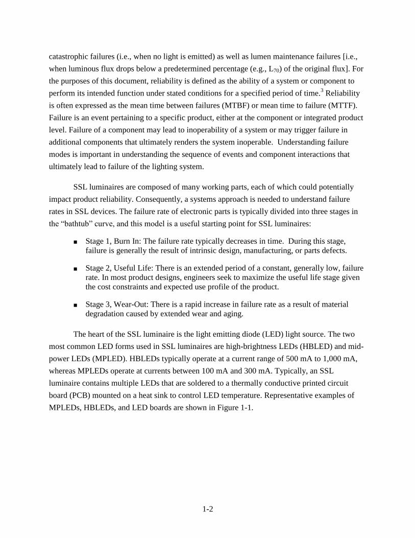
The heart of the SSL luminaire is the light emitting diode (LED) light source. The two
most common LED forms used in SSL luminaires are high-brightness LEDs (HBLED) and mid-
power LEDs (MPLED). HBLEDs typically operate at a current range of 500 mA to 1,000 mA,
whereas MPLEDs operate at currents between 100 mA and 300 mA. Typically, an SSL
luminaire contains multiple LEDs that are soldered to a thermally conductive printed circuit
board (PCB) mounted on a heat sink to control LED temperature. Representative examples of
MPLEDs, HBLEDs, and LED boards are shown in Figure 1-1.
1-3
Figure 1-1. Representative Examples of LEDs Used in Lighting
The LED types are MPLED, LED array, and HBLED from left to right. All of the LEDs are shown
mounted on a PCB.
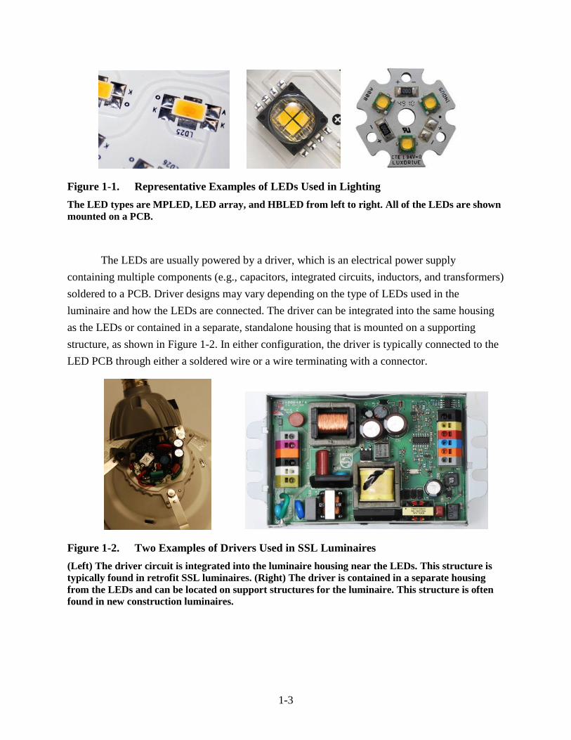
The LEDs are usually powered by a driver, which is an electrical power supply
containing multiple components (e.g., capacitors, integrated circuits, inductors, and transformers)
soldered to a PCB. Driver designs may vary depending on the type of LEDs used in the
luminaire and how the LEDs are connected. The driver can be integrated into the same housing
as the LEDs or contained in a separate, standalone housing that is mounted on a supporting
structure, as shown in Figure 1-2. In either configuration, the driver is typically connected to the
LED PCB through either a soldered wire or a wire terminating with a connector.
Figure 1-2. Two Examples of Drivers Used in SSL Luminaires
(Left) The driver circuit is integrated into the luminaire housing near the LEDs. This structure is
typically found in retrofit SSL luminaires. (Right) The driver is contained in a separate housing
from the LEDs and can be located on support structures for the luminaire. This structure is often
found in new construction luminaires.
1-4
Assuming that luminaire failure occurs at a constant rate, the fraction of the luminaire
population failing at time t can be defined as follows: 4
F(t) = 1– exp(–t/) (1.1)
where
F(t) is the population fraction failing at time t,
t is time, and
is the MTBF.
For a system comprised of multiple components, assuming no interactions between components:
Fsys(t) = F1(t)F2(t)…Fn(t) (1.2)
where
Fsys(t) is the population fraction of the entire system failing at time t, and
F1(t) to Fn(t) is the population fraction of component 1, 2, …, n failing at time t. An
example of the impact of component failure probabilities on the overall system failure
probability can be found elsewhere.3
Alternatively, a reliability function R(t) can be defined for a life distribution, where R(t)
represents the probability of survival beyond age t. R(t) is also called the survivor or survivorship
function and is related to F(t) in a straightforward fashion:4
R(t) = 1 – F(t) (1.3)
For simplicity, the time dependence of R and F are dropped for the remainder of the
document. Since the major components of SSL luminaires include the LEDs, optics, reflectors,
and diffusers—and assuming that these elements operate in series—the reliability function (Rlum)
of the SSL luminaire is the product of the major component reliability functions:
Rlum = RLEDRDrivROpticsRRefRother (1.4)
Where the LED reliability function is given by RLED, the driver reliability function is
given by RDriv, the optics reliability function is given by ROptics, the reflector reliability function is
given by RRef , and the reliability of the remainder of the system is given by Rother. Additional
information on the components of SSL luminaires is provided in Table 1-1.
4 For more information see Wayne B. Nelson, Accelerated Testing: Statistical Models, Test Plans, and Data
Analysis, Wiley Interscience (2004) Hoboken, New Jersey.
1-5
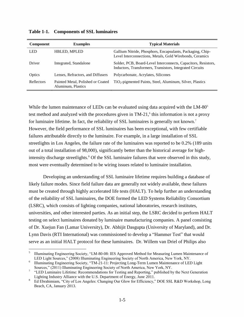
Table 1-1. Components of SSL luminaires
Component Examples Typical Materials
LED HBLED, MPLED Gallium Nitride, Phosphors, Encapsulants, Packaging, Chip-
Level Interconnections, Metals, Gold Wirebonds, Ceramics
Driver Integrated, Standalone Solder, PCB, Board-Level Interconnects, Capacitors, Resistors,
Inductors, Transformers, Transistors, Integrated Circuits
Optics Lenses, Refractors, and Diffusers Polycarbonate, Acrylates, Silicones
Reflectors Painted Metal, Polished or Coated
Aluminum, Plastics
TiO2-pigmented Paints, Steel, Aluminum, Silver, Plastics
While the lumen maintenance of LEDs can be evaluated using data acquired with the LM-805
test method and analyzed with the procedures given in TM-21,6 this information is not a proxy
for luminaire lifetime. In fact, the reliability of SSL luminaires is generally not known.7
However, the field performance of SSL luminaires has been exceptional, with few certifiable
failures attributable directly to the luminaire. For example, in a large installation of SSL
streetlights in Los Angeles, the failure rate of the luminaires was reported to be 0.2% (189 units
out of a total installation of 98,000), significantly better than the historical average for high-
intensity discharge streetlights.8 Of the SSL luminaire failures that were observed in this study,
most were eventually determined to be wiring issues related to luminaire installation.
Developing an understanding of SSL luminaire lifetime requires building a database of
likely failure modes. Since field failure data are generally not widely available, these failures
must be created through highly accelerated life tests (HALT). To help further an understanding
of the reliability of SSL luminaires, the DOE formed the LED Systems Reliability Consortium
(LSRC), which consists of lighting companies, national laboratories, research institutes,
universities, and other interested parties. As an initial step, the LSRC decided to perform HALT
testing on select luminaires donated by luminaire manufacturing companies. A panel consisting
of Dr. Xuejun Fan (Lamar University), Dr. Abhijit Dasgupta (University of Maryland), and Dr.
Lynn Davis (RTI International) was commissioned to develop a “Hammer Test” that would
serve as an initial HALT protocol for these luminaires. Dr. Willem van Driel of Philips also
5 Illuminating Engineering Society, “LM-80-08: IES Approved Method for Measuring Lumen Maintenance of
LED Light Sources,” (2008) Illuminating Engineering Society of North America, New York, NY. 6 Illuminating Engineering Society, “TM-21-11: Projecting Long-Term Lumen Maintenance of LED Light
Sources,” (2011) Illuminating Engineering Society of North America, New York, NY. 7 “LED Luminaire Lifetime: Recommendations for Testing and Reporting,” published by the Next Generation
Lighting Industry Alliance with the U.S. Department of Energy, June 2011. 8 Ed Ebrahimiam, “City of Los Angeles: Changing Our Glow for Efficiency,” DOE SSL R&D Workshop, Long
Beach, CA, January 2013.
1-6
provided valuable inputs to the panel. The Hammer Test was to serve as a HALT method that
would produce failures in SSL luminaires in a reasonable test period (defined as less than 2,000
hours of testing). It was not intended to be a universal accelerated life test (ALT) for luminaires,
but instead was designed solely to provide insights into potential failure modes. Once identified,
these failure modes could be studied in a more quantitative fashion than is possible with a rapid
screening protocol such as the Hammer Test.
This report provides findings from the LSRC Hammer Test on seven commercial SSL
luminaires. Section 1 provides background information. Section 2 provides details on the
Hammer Test protocols and the measurement procedures that were used to evaluate the
luminaires. Section 3 provides details on the luminaires undergoing testing. Section 4 provides
details on the experimental findings, and Section 5 presents a discussion of those findings.
Section 6 concludes the report and provides insights for additional studies.
2-1
SECTION 2
TEST METHODS
2.1 Hammer Test Procedures
One loop of the Hammer Test consists of four stages of different environmental stresses,
and each stage was modeled after common stress tests used in the electronics industry.
Cumulatively, one loop of the Hammer Test lasts for 42 hours, with each stage presenting a
stress comprising variations in heat and humidity. Electrical power was cycled on and off during
the Hammer Test as described below. The Hammer Test provides an extreme stress environment
for the luminaires, and the testing protocol is intended to create failures in a reasonable period of
time. These failures can provide qualitative information on potential field failure modes in SSL
luminaires that can be studied in more depth using more quantitative ALTs.
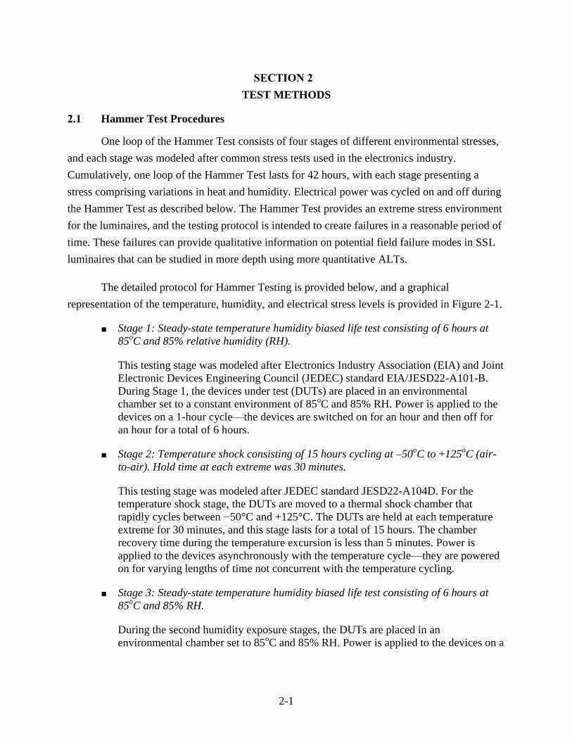
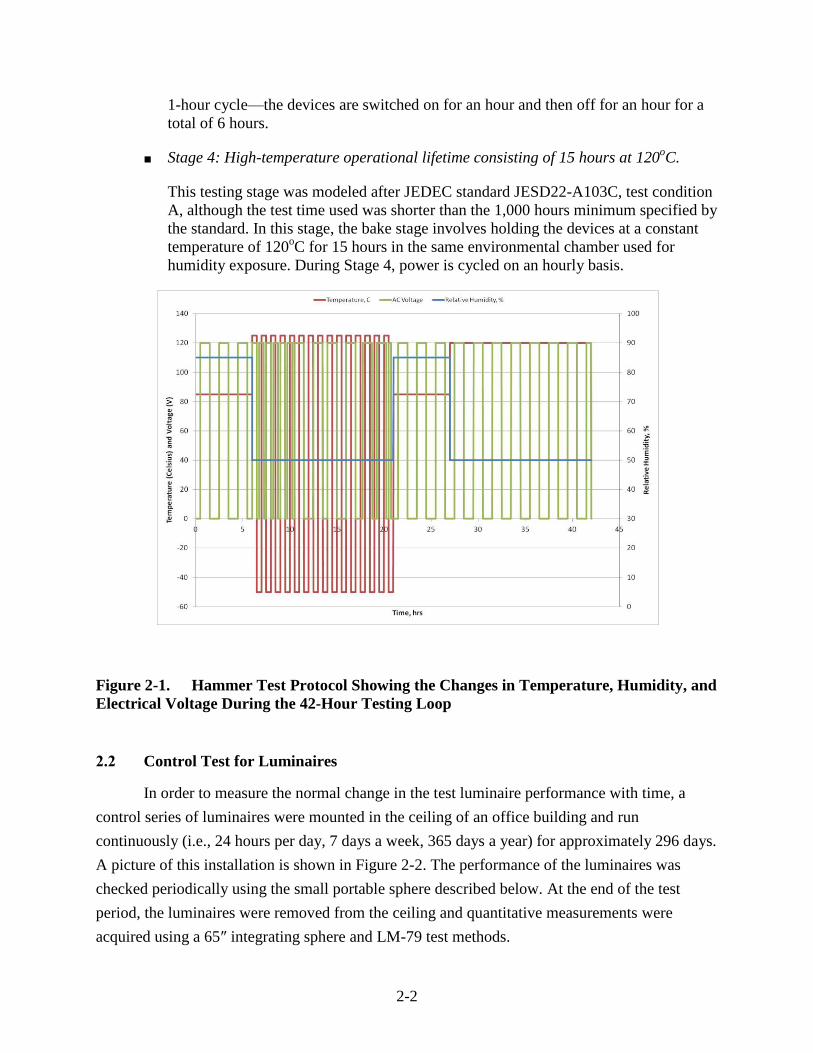
The detailed protocol for Hammer Testing is provided below, and a graphical
representation of the temperature, humidity, and electrical stress levels is provided in Figure 2-1.
■ Stage 1: Steady-state temperature humidity biased life test consisting of 6 hours at
85oC and 85% relative humidity (RH).
This testing stage was modeled after Electronics Industry Association (EIA) and Joint
Electronic Devices Engineering Council (JEDEC) standard EIA/JESD22-A101-B.
During Stage 1, the devices under test (DUTs) are placed in an environmental
chamber set to a constant environment of 85oC and 85% RH. Power is applied to the
devices on a 1-hour cycle—the devices are switched on for an hour and then off for
an hour for a total of 6 hours.
■ Stage 2: Temperature shock consisting of 15 hours cycling at –50oC to +125
oC (air-
to-air). Hold time at each extreme was 30 minutes.
This testing stage was modeled after JEDEC standard JESD22-A104D. For the
temperature shock stage, the DUTs are moved to a thermal shock chamber that
rapidly cycles between −50°C and +125°C. The DUTs are held at each temperature
extreme for 30 minutes, and this stage lasts for a total of 15 hours. The chamber
recovery time during the temperature excursion is less than 5 minutes. Power is
applied to the devices asynchronously with the temperature cycle—they are powered
on for varying lengths of time not concurrent with the temperature cycling.
■ Stage 3: Steady-state temperature humidity biased life test consisting of 6 hours at
85oC and 85% RH.
During the second humidity exposure stages, the DUTs are placed in an
environmental chamber set to 85oC and 85% RH. Power is applied to the devices on a
2-2
1-hour cycle—the devices are switched on for an hour and then off for an hour for a
total of 6 hours.
■ Stage 4: High-temperature operational lifetime consisting of 15 hours at 120oC.
This testing stage was modeled after JEDEC standard JESD22-A103C, test condition
A, although the test time used was shorter than the 1,000 hours minimum specified by
the standard. In this stage, the bake stage involves holding the devices at a constant
temperature of 120oC for 15 hours in the same environmental chamber used for
humidity exposure. During Stage 4, power is cycled on an hourly basis.
Figure 2-1. Hammer Test Protocol Showing the Changes in Temperature, Humidity, and
Electrical Voltage During the 42-Hour Testing Loop
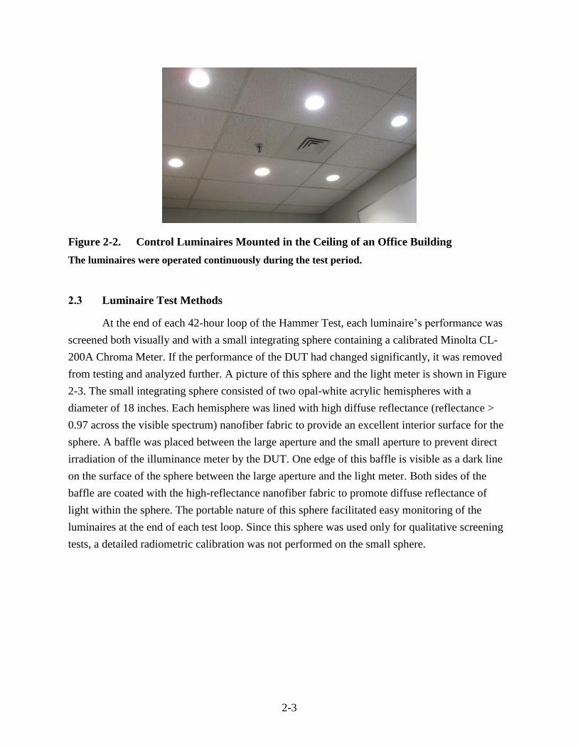
2.2 Control Test for Luminaires
In order to measure the normal change in the test luminaire performance with time, a
control series of luminaires were mounted in the ceiling of an office building and run
continuously (i.e., 24 hours per day, 7 days a week, 365 days a year) for approximately 296 days.
A picture of this installation is shown in Figure 2-2. The performance of the luminaires was
checked periodically using the small portable sphere described below. At the end of the test
period, the luminaires were removed from the ceiling and quantitative measurements were
acquired using a 65″ integrating sphere and LM-79 test methods.
2-3
Figure 2-2. Control Luminaires Mounted in the Ceiling of an Office Building
The luminaires were operated continuously during the test period.
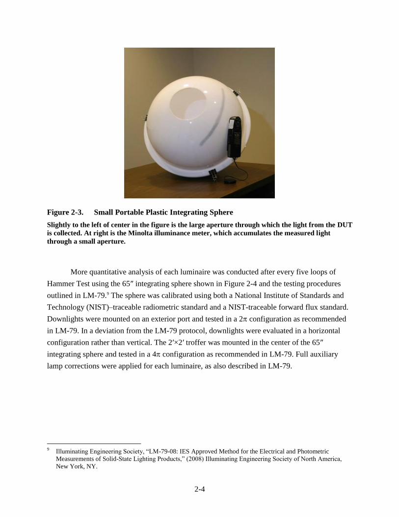
2.3 Luminaire Test Methods
At the end of each 42-hour loop of the Hammer Test, each luminaire’s performance was
screened both visually and with a small integrating sphere containing a calibrated Minolta CL-
200A Chroma Meter. If the performance of the DUT had changed significantly, it was removed
from testing and analyzed further. A picture of this sphere and the light meter is shown in Figure
2-3. The small integrating sphere consisted of two opal-white acrylic hemispheres with a
diameter of 18 inches. Each hemisphere was lined with high diffuse reflectance (reflectance >
0.97 across the visible spectrum) nanofiber fabric to provide an excellent interior surface for the
sphere. A baffle was placed between the large aperture and the small aperture to prevent direct
irradiation of the illuminance meter by the DUT. One edge of this baffle is visible as a dark line
on the surface of the sphere between the large aperture and the light meter. Both sides of the
baffle are coated with the high-reflectance nanofiber fabric to promote diffuse reflectance of
light within the sphere. The portable nature of this sphere facilitated easy monitoring of the
luminaires at the end of each test loop. Since this sphere was used only for qualitative screening
tests, a detailed radiometric calibration was not performed on the small sphere.
2-4
Figure 2-3. Small Portable Plastic Integrating Sphere
Slightly to the left of center in the figure is the large aperture through which the light from the DUT
is collected. At right is the Minolta illuminance meter, which accumulates the measured light
through a small aperture.
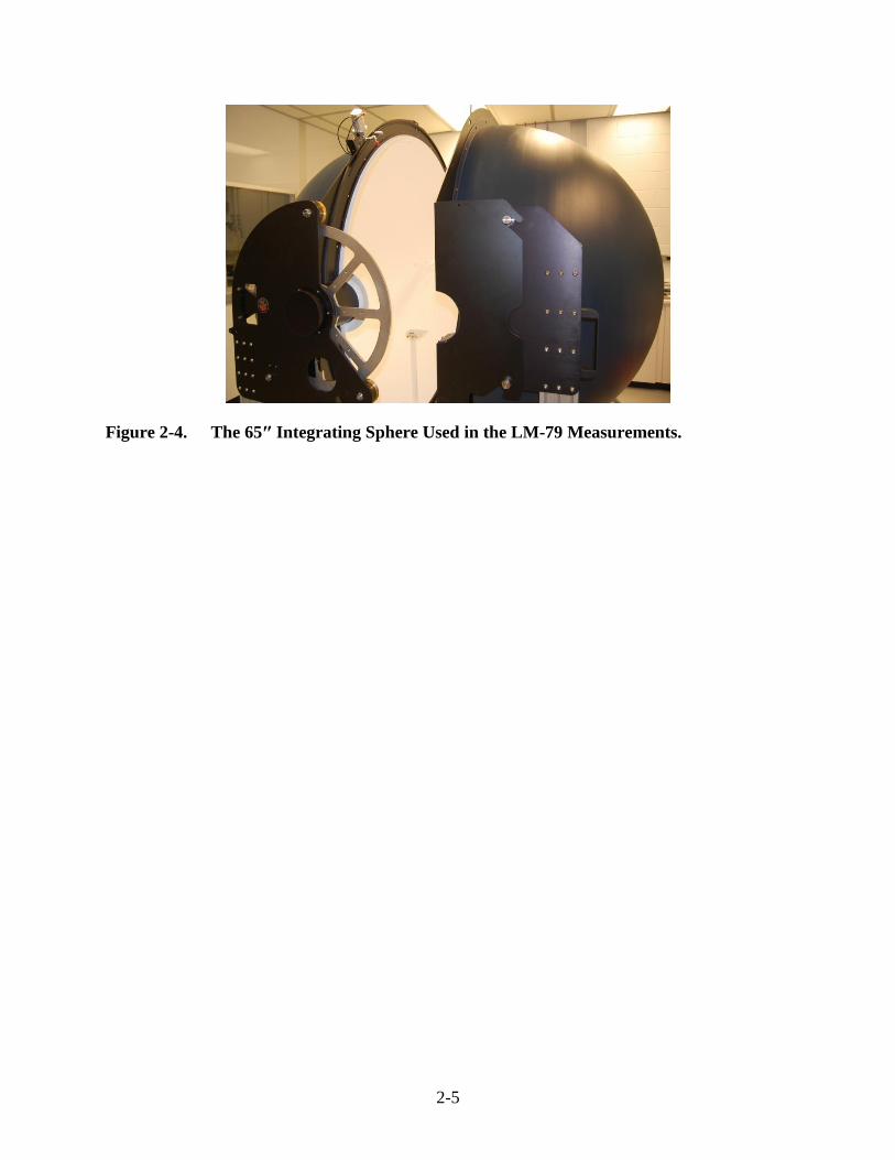
More quantitative analysis of each luminaire was conducted after every five loops of
Hammer Test using the 65″ integrating sphere shown in Figure 2-4 and the testing procedures
outlined in LM-79.9 The sphere was calibrated using both a National Institute of Standards and
Technology (NIST)–traceable radiometric standard and a NIST-traceable forward flux standard.
Downlights were mounted on an exterior port and tested in a 2 configuration as recommended
in LM-79. In a deviation from the LM-79 protocol, downlights were evaluated in a horizontal
configuration rather than vertical. The 2′×2′ troffer was mounted in the center of the 65″
integrating sphere and tested in a 4 configuration as recommended in LM-79. Full auxiliary
lamp corrections were applied for each luminaire, as also described in LM-79.
9 Illuminating Engineering Society, “LM-79-08: IES Approved Method for the Electrical and Photometric
Measurements of Solid-State Lighting Products,” (2008) Illuminating Engineering Society of North America,
New York, NY.
2-5
Figure 2-4. The 65″ Integrating Sphere Used in the LM-79 Measurements.
3-1
SECTION 3
LUMINAIRES UNDER TEST
Seven different commercial luminaire models, provided by different manufacturers or
independently purchased, were examined during the Hammer Test. Six of the luminaire models
were 6″ downlights or similar products, and one luminaire model was a 2′×2′ troffer. Because of
the large number of different products in the Hammer Test, only a limited number of samples for
each product could be tested. Typically, three samples of each product were included in the
Hammer Test, although some products had fewer test samples.
The tested group of luminaires included many common variations often encountered in
SSL products. For example, a variety of LED configurations was included in the test: four
phosphor-converted LED (pcLED) designs, one remote phosphor design, and two hybrid LED
designs. The downlights that were tested also contained a variety of construction practices,
including different reflector and optical materials and variations in the size and structure of an
optical mixing cavity. Four of the six downlights were retrofit models containing Edison E26
screw bases (NEMA ANSI C78.20:2003), plugs, and integrated power supplies. Two of the
downlights and the troffer were new construction luminaires with the driver physically separated
from the luminaire. The location of the driver may have an effect on reliability, depending on the
potential heat that can be transferred from the LEDs to the driver board when they are in
proximity. As a general rule, the retrofit products that were tested tended to be lower power than
the new construction luminaires, and the lower power consumption allowed the use of the
product housing for heat dissipation. Both of the new construction downlights had large heat
sinks to facilitate heat dissipation. Additional details on the luminaires examined in the Hammer
Test are provided in Table 3-1. To preserve the confidentiality of the various manufacturers and
their products, the luminaires and LEDs are identified with codes (e.g., Luminaire A, Luminaire
B) for the remainder of this report.
3-2
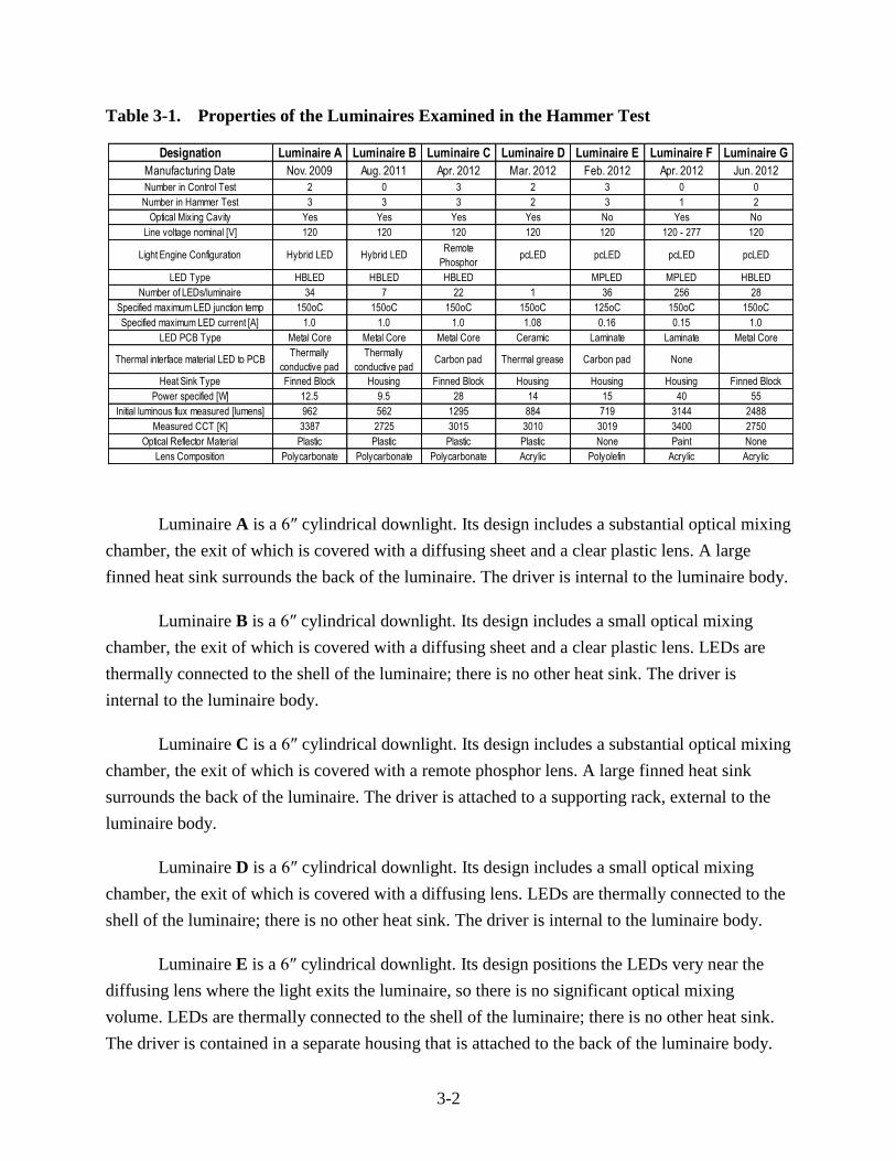
Table 3-1. Properties of the Luminaires Examined in the Hammer Test
Luminaire A is a 6″ cylindrical downlight. Its design includes a substantial optical mixing
chamber, the exit of which is covered with a diffusing sheet and a clear plastic lens. A large
finned heat sink surrounds the back of the luminaire. The driver is internal to the luminaire body.
Luminaire B is a 6″ cylindrical downlight. Its design includes a small optical mixing
chamber, the exit of which is covered with a diffusing sheet and a clear plastic lens. LEDs are
thermally connected to the shell of the luminaire; there is no other heat sink. The driver is
internal to the luminaire body.
Luminaire C is a 6″ cylindrical downlight. Its design includes a substantial optical mixing
chamber, the exit of which is covered with a remote phosphor lens. A large finned heat sink
surrounds the back of the luminaire. The driver is attached to a supporting rack, external to the
luminaire body.
Luminaire D is a 6″ cylindrical downlight. Its design includes a small optical mixing
chamber, the exit of which is covered with a diffusing lens. LEDs are thermally connected to the
shell of the luminaire; there is no other heat sink. The driver is internal to the luminaire body.
Luminaire E is a 6″ cylindrical downlight. Its design positions the LEDs very near the
diffusing lens where the light exits the luminaire, so there is no significant optical mixing
volume. LEDs are thermally connected to the shell of the luminaire; there is no other heat sink.
The driver is contained in a separate housing that is attached to the back of the luminaire body.
Designation Luminaire A Luminaire B Luminaire C Luminaire D Luminaire E Luminaire F Luminaire G
Manufacturing Date Nov. 2009 Aug. 2011 Apr. 2012 Mar. 2012 Feb. 2012 Apr. 2012 Jun. 2012
Number in Control Test 2 0 3 2 3 0 0
Number in Hammer Test 3 3 3 2 3 1 2
Optical Mixing Cavity Yes Yes Yes Yes No Yes No
Line voltage nominal [V] 120 120 120 120 120 120 - 277 120
Light Engine Configuration Hybrid LED Hybrid LEDRemote
PhosphorpcLED pcLED pcLED pcLED
LED Type HBLED HBLED HBLED MPLED MPLED HBLED
Number of LEDs/luminaire 34 7 22 1 36 256 28
Specified maximum LED junction temp 150oC 150oC 150oC 150oC 125oC 150oC 150oC
Specified maximum LED current [A] 1.0 1.0 1.0 1.08 0.16 0.15 1.0
LED PCB Type Metal Core Metal Core Metal Core Ceramic Laminate Laminate Metal Core
Thermal interface material LED to PCBThermally
conductive pad
Thermally
conductive padCarbon pad Thermal grease Carbon pad None
Heat Sink Type Finned Block Housing Finned Block Housing Housing Housing Finned Block
Power specified [W] 12.5 9.5 28 14 15 40 55
Initial luminous flux measured [lumens] 962 562 1295 884 719 3144 2488
Measured CCT [K] 3387 2725 3015 3010 3019 3400 2750
Optical Reflector Material Plastic Plastic Plastic Plastic None Paint None
Lens Composition Polycarbonate Polycarbonate Polycarbonate Acrylic Polyolefin Acrylic Acrylic
3-3
Luminaire F is a 2′×2′ troffer containing a large number of mid-power pcLEDs. The pan
of the luminaire is covered by a diffusing white plastic lens at the light exit. The LEDs are
attached to boards connected to the luminaire pan, providing a large surface area without any
additional heat sinks. The separation between the diffusing lens and the LEDs is roughly 1.5″
providing a substantial optical mixing volume. The driver is contained in a separate housing that
is attached to the back of the luminaire body.
Luminaire G is a 6″ cylindrical downlight. LEDs are positioned to deliver illumination to
the exterior through transparent lenses, so there is no optical mixing volume. A large finned heat
sink surrounds the back of the luminaire. The driver is attached to a supporting rack, external to
the luminaire body.
4-1
SECTION 4
TEST RESULTS
4.1 Test Results for Control Luminaires
The total sample populations of Luminaires A, C, D, and E were split; half (typically
three samples each) were placed into the Hammer Test and the other half were used as controls.
As discussed in Section 2.2, the control luminaires were placed in the ceiling of an office
building and operated continuously for 296 days. The luminaires were mounted in accordance
with manufacturer’s recommendations. The typical conditions of the office building were a
nominal heating, ventilation, and air conditioning (HVAC) controlled office environment with an
ambient temperature of 22oC between 7 a.m. and 6 p.m. Outside of those times, the HVAC
system was cut back through automatic dampers and the temperature may have changed slightly,
but the change was typically less than 5°C.
Assuming a typical office usage profile where the lights are on for 12 hours per day for
260 days per years (i.e., 5 days per week for 52 weeks), this control test profile roughly
corresponds to 2.25 years of operation. A slight difference between the typical usage profile and
this control group is that the duty cycle of the control group is essentially zero since the control
luminaires are only turned off when the power to the office is interrupted. In contrast, luminaires
in a typical office building are usually turned on and off once a day. Such a low-duty cycle is not
believed to have a significant impact on luminaire reliability, so this difference is ignored in this
report.
The performance of the control luminaires was regularly checked during operation using
the small portable integrating sphere shown in Figure 2-3. During these period inspections, the
variation in measured illuminance remained within 6% of the initial value. Since this inspection
was intended to be qualitative in nature, this finding was taken as an indication that no large
changes were occurring in the performance of control luminaires during the first test period.
After approximately 7,100 hours of continuous operation, the luminaires were removed
from the ceiling and photometric testing was performed on each unit in a 65″ integrating sphere.
The luminaires were allowed to warm up for a minimum of 1 hour prior to testing, in accordance
with guidelines given in LM-79. The test results are shown in Table 4-1.
4-2
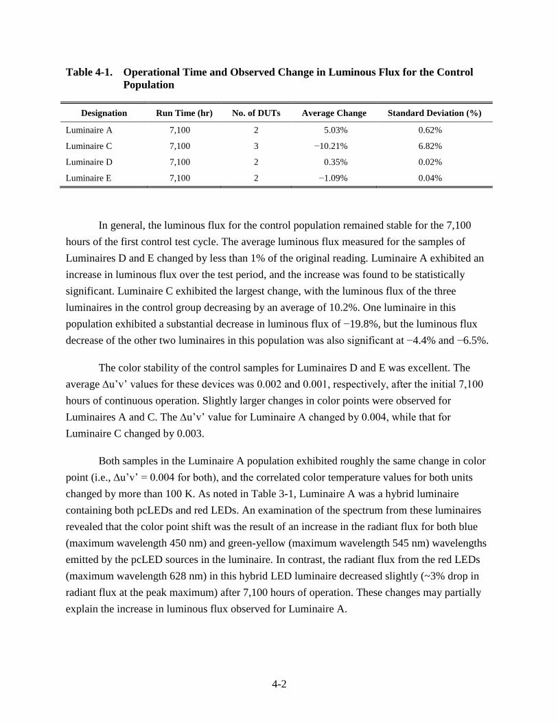
Table 4-1. Operational Time and Observed Change in Luminous Flux for the Control
Population
Designation Run Time (hr) No. of DUTs Average Change Standard Deviation (%)
Luminaire A 7,100 2 5.03% 0.62%
Luminaire C 7,100 3 −10.21% 6.82%
Luminaire D 7,100 2 0.35% 0.02%
Luminaire E 7,100 2 −1.09% 0.04%
In general, the luminous flux for the control population remained stable for the 7,100
hours of the first control test cycle. The average luminous flux measured for the samples of
Luminaires D and E changed by less than 1% of the original reading. Luminaire A exhibited an
increase in luminous flux over the test period, and the increase was found to be statistically
significant. Luminaire C exhibited the largest change, with the luminous flux of the three
luminaires in the control group decreasing by an average of 10.2%. One luminaire in this
population exhibited a substantial decrease in luminous flux of −19.8%, but the luminous flux
decrease of the other two luminaires in this population was also significant at −4.4% and −6.5%.
The color stability of the control samples for Luminaires D and E was excellent. The
average u’v’ values for these devices was 0.002 and 0.001, respectively, after the initial 7,100
hours of continuous operation. Slightly larger changes in color points were observed for
Luminaires A and C. The u’v’ value for Luminaire A changed by 0.004, while that for
Luminaire C changed by 0.003.
Both samples in the Luminaire A population exhibited roughly the same change in color
point (i.e., u’v’ = 0.004 for both), and the correlated color temperature values for both units
changed by more than 100 K. As noted in Table 3-1, Luminaire A was a hybrid luminaire
containing both pcLEDs and red LEDs. An examination of the spectrum from these luminaires
revealed that the color point shift was the result of an increase in the radiant flux for both blue
(maximum wavelength 450 nm) and green-yellow (maximum wavelength 545 nm) wavelengths
emitted by the pcLED sources in the luminaire. In contrast, the radiant flux from the red LEDs
(maximum wavelength 628 nm) in this hybrid LED luminaire decreased slightly (~3% drop in
radiant flux at the peak maximum) after 7,100 hours of operation. These changes may partially
explain the increase in luminous flux observed for Luminaire A.
4-3
4.2 Summary of Hammer Test Results
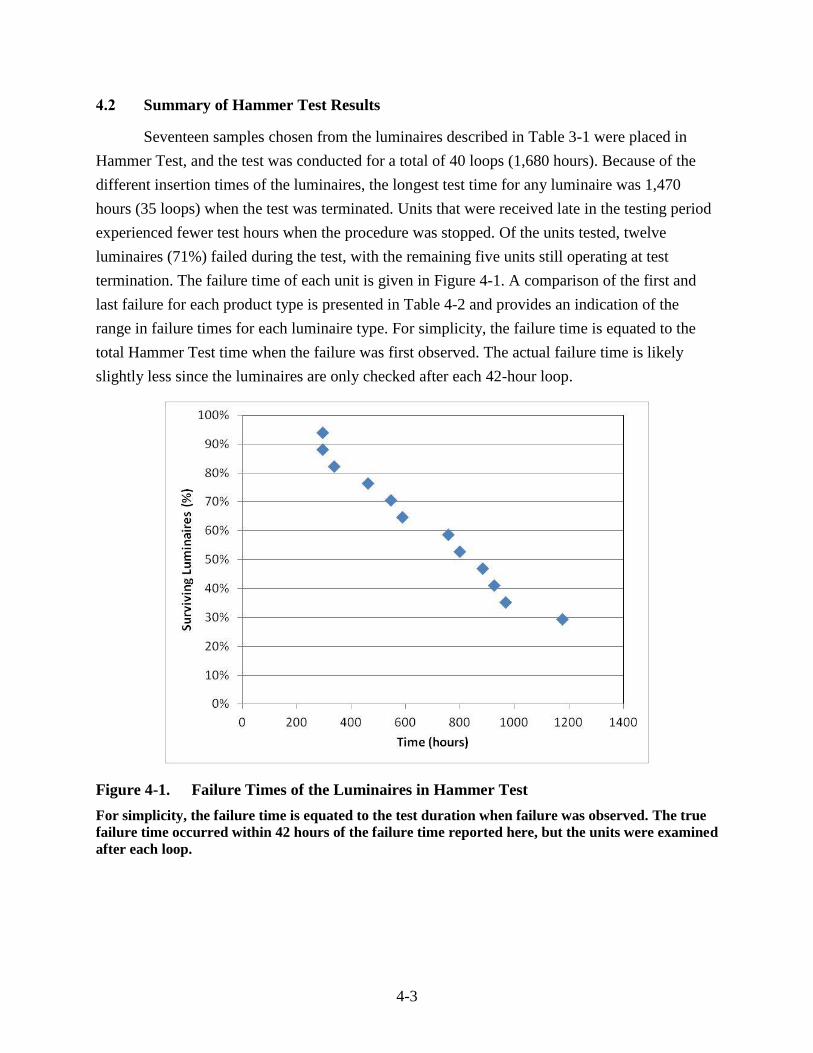
Seventeen samples chosen from the luminaires described in Table 3-1 were placed in
Hammer Test, and the test was conducted for a total of 40 loops (1,680 hours). Because of the
different insertion times of the luminaires, the longest test time for any luminaire was 1,470
hours (35 loops) when the test was terminated. Units that were received late in the testing period
experienced fewer test hours when the procedure was stopped. Of the units tested, twelve
luminaires (71%) failed during the test, with the remaining five units still operating at test
termination. The failure time of each unit is given in Figure 4-1. A comparison of the first and
last failure for each product type is presented in Table 4-2 and provides an indication of the
range in failure times for each luminaire type. For simplicity, the failure time is equated to the
total Hammer Test time when the failure was first observed. The actual failure time is likely
slightly less since the luminaires are only checked after each 42-hour loop.
Figure 4-1. Failure Times of the Luminaires in Hammer Test
For simplicity, the failure time is equated to the test duration when failure was observed. The true
failure time occurred within 42 hours of the failure time reported here, but the units were examined
after each loop.
4-4
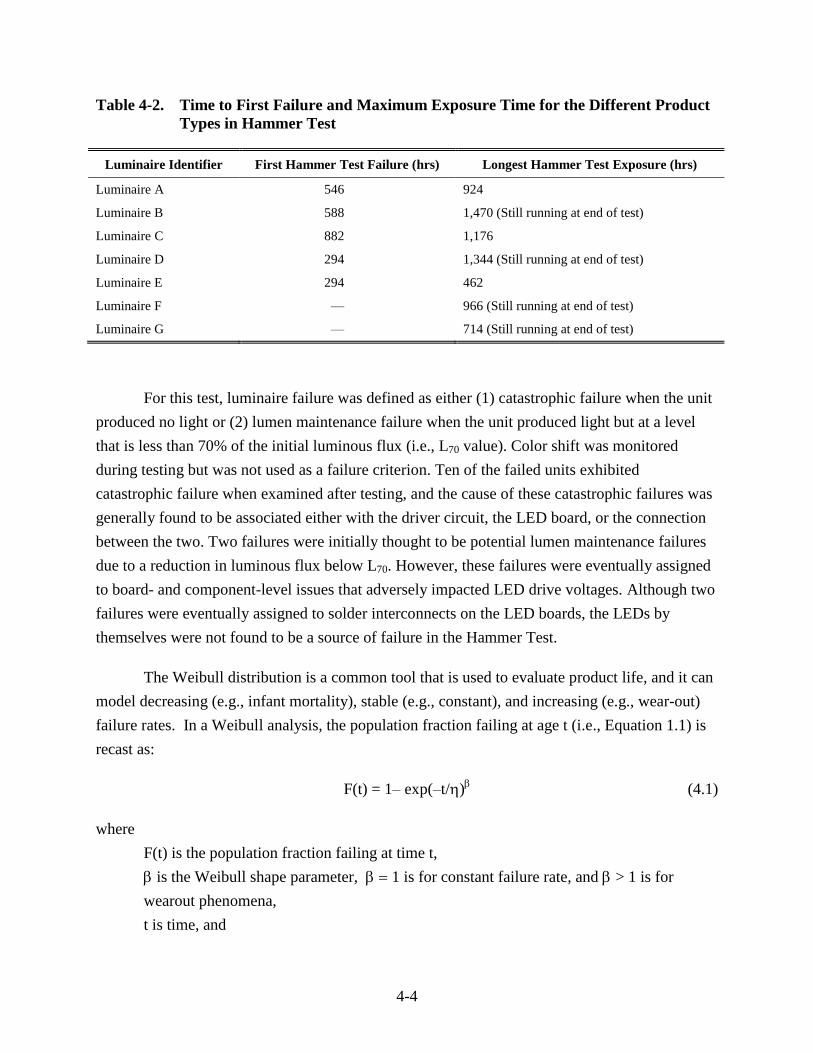
Table 4-2. Time to First Failure and Maximum Exposure Time for the Different Product
Types in Hammer Test
Luminaire Identifier First Hammer Test Failure (hrs) Longest Hammer Test Exposure (hrs)
Luminaire A 546 924
Luminaire B 588 1,470 (Still running at end of test)
Luminaire C 882 1,176
Luminaire D 294 1,344 (Still running at end of test)
Luminaire E 294 462
Luminaire F — 966 (Still running at end of test)
Luminaire G — 714 (Still running at end of test)
For this test, luminaire failure was defined as either (1) catastrophic failure when the unit
produced no light or (2) lumen maintenance failure when the unit produced light but at a level
that is less than 70% of the initial luminous flux (i.e., L70 value). Color shift was monitored
during testing but was not used as a failure criterion. Ten of the failed units exhibited
catastrophic failure when examined after testing, and the cause of these catastrophic failures was
generally found to be associated either with the driver circuit, the LED board, or the connection
between the two. Two failures were initially thought to be potential lumen maintenance failures
due to a reduction in luminous flux below L70. However, these failures were eventually assigned
to board- and component-level issues that adversely impacted LED drive voltages. Although two
failures were eventually assigned to solder interconnects on the LED boards, the LEDs by
themselves were not found to be a source of failure in the Hammer Test.
The Weibull distribution is a common tool that is used to evaluate product life, and it can
model decreasing (e.g., infant mortality), stable (e.g., constant), and increasing (e.g., wear-out)
failure rates. In a Weibull analysis, the population fraction failing at age t (i.e., Equation 1.1) is
recast as:
F(t) = 1– exp(–t/) (4.1)
where
F(t) is the population fraction failing at time t,
is the Weibull shape parameter, 1 is for constant failure rate, and > 1 is for
wearout phenomena,
t is time, and
4-5
is the Weibull scale parameter (aka, characteristic life). provides an indication of the
width of the failure distribution, assuming a constant .
In a typical Weibull analysis, the fraction of the population failure (i.e, F(t)) is plotted against
time in a log-log graph The slope of the plot gives the value of , and the value at 63.2% gives
the value of .
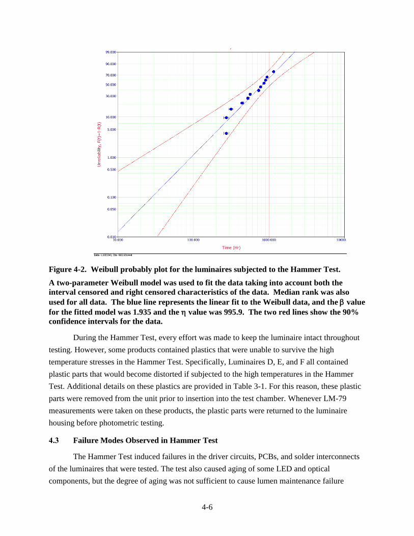
The data provided in Figure 4-1 can also be recast as a Weibull probability plot, as
shown in Figure 4-2. A two-parameter Weibull model was used to fit the data, and maximum
likelihood estimator methods were used to account for censored data. Since the performance of
the luminaires are tested before each loop of the Hammer Test and their continued performance
(or lack thereof) is verified after each loop (i.e., after 42 hours of testing), the exact failure time
is unknown. This prompted the data to be treated as interval censored data for all failures in the
Weibull analysis. Devices that were still operational at the end of the Hammer Test were treated
as right censored data. Median rank methods were applied to the censored data. This treatment
of the data resulted in the following parameters for the Weibull model:
Shape parameter () = 1.935
Scale parameter () = 995.9
Since the value was greater than 1, wearout phenomena are responsible for the failure of the
luminaires. This observed value of demonstrates that the Hammer Test is an acceleration test.
4-6
Figure 4-2. Weibull probably plot for the luminaires subjected to the Hammer Test.
A two-parameter Weibull model was used to fit the data taking into account both the
interval censored and right censored characteristics of the data. Median rank was also
used for all data. The blue line represents the linear fit to the Weibull data, and the value
for the fitted model was 1.935 and the value was 995.9. The two red lines show the 90%
confidence intervals for the data.
During the Hammer Test, every effort was made to keep the luminaire intact throughout
testing. However, some products contained plastics that were unable to survive the high
temperature stresses in the Hammer Test. Specifically, Luminaires D, E, and F all contained
plastic parts that would become distorted if subjected to the high temperatures in the Hammer
Test. Additional details on these plastics are provided in Table 3-1. For this reason, these plastic
parts were removed from the unit prior to insertion into the test chamber. Whenever LM-79
measurements were taken on these products, the plastic parts were returned to the luminaire
housing before photometric testing.
4.3 Failure Modes Observed in Hammer Test
The Hammer Test induced failures in the driver circuits, PCBs, and solder interconnects
of the luminaires that were tested. The test also caused aging of some LED and optical
components, but the degree of aging was not sufficient to cause lumen maintenance failure
4-7
during the test interval. A closer examination of Table 4-2 reveals the range in failure times that
was observed for the various luminaires in testing. For example, the failures for Luminaire E
occurred in a narrow time window between 294 and 462 hours. This finding can be anticipated
from the luminaire design specification and the LED operation specification for these products.
These failures may be examples of product wear-out that was accelerated by the extreme
conditions of the Hammer Test. In contrast, one unit from Luminaire D failed early in the
Hammer Test (294 hours), while the other unit was still operational at the termination of the test
(total exposure time of 1,344 hours). In this instance, the early failure is likely not due to a wear-
out mechanism. The Hammer Test failure times for the other products also showed some
variability. Since the primary goal of the Hammer Test is to identify potential failure modes and
not to compare the reliability of various products, additional study of the products is warranted to
understand the failure modes caused by the severe environmental stresses of the Hammer Test
and to determine acceleration factors. Such studies, which are beyond the scope of this initial
effort, are required to estimate reliability and lifetime.
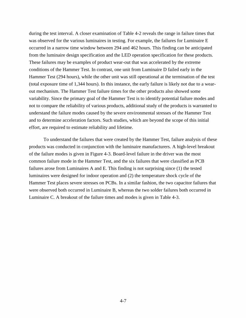
To understand the failures that were created by the Hammer Test, failure analysis of these
products was conducted in conjunction with the luminaire manufacturers. A high-level breakout
of the failure modes is given in Figure 4-3. Board-level failure in the driver was the most
common failure mode in the Hammer Test, and the six failures that were classified as PCB
failures arose from Luminaires A and E. This finding is not surprising since (1) the tested
luminaires were designed for indoor operation and (2) the temperature shock cycle of the
Hammer Test places severe stresses on PCBs. In a similar fashion, the two capacitor failures that
were observed both occurred in Luminaire B, whereas the two solder failures both occurred in
Luminaire C. A breakout of the failure times and modes is given in Table 4-3.
4-8
Figure 4-3. Distribution of Failure Modes for Luminaires Examined During the Hammer
Test
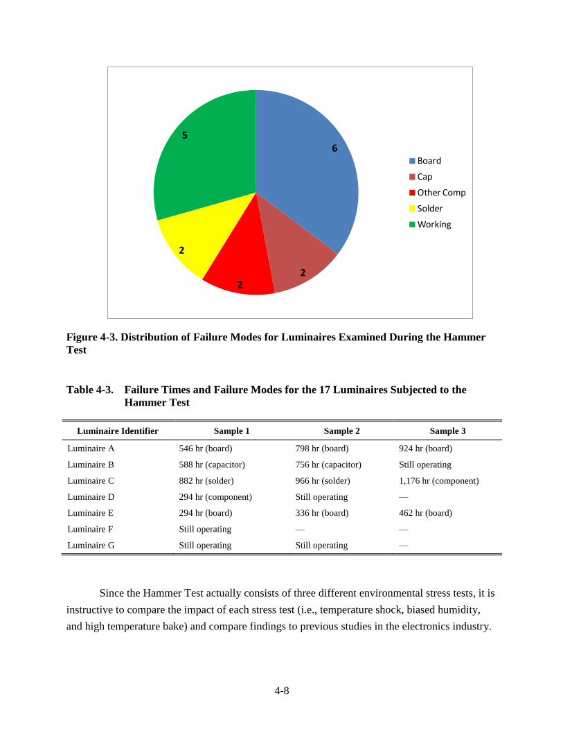
Table 4-3. Failure Times and Failure Modes for the 17 Luminaires Subjected to the
Hammer Test
Luminaire Identifier Sample 1 Sample 2 Sample 3
Luminaire A 546 hr (board) 798 hr (board) 924 hr (board)
Luminaire B 588 hr (capacitor) 756 hr (capacitor) Still operating
Luminaire C 882 hr (solder) 966 hr (solder) 1,176 hr (component)
Luminaire D 294 hr (component) Still operating —
Luminaire E 294 hr (board) 336 hr (board) 462 hr (board)
Luminaire F Still operating — —
Luminaire G Still operating Still operating —
Since the Hammer Test actually consists of three different environmental stress tests, it is
instructive to compare the impact of each stress test (i.e., temperature shock, biased humidity,
and high temperature bake) and compare findings to previous studies in the electronics industry.
6
22
2
5
Board
Cap
Other Comp
Solder
Working
4-9
The following sections examine each stress and previous work on the impact of the individual
stress test and their impact on the luminaires.
4.3.1 Temperature Cycling (−50°C to 125°C)
The temperature cycling regimen in the Hammer Test is intended to determine the ability
of components, PCBs, and solder interconnects to withstand the mechanical stresses that arise
with rapid cycling between low and high temperature extremes. For indoor luminaires, the
temperature cycling of a device will typically be between 15°C (when the device is off) to as
much as 60°C when the device is operating, although wider temperature extremes are possible.
For outdoor luminaires, the temperature excursion could be much larger, possibly spanning that
range from −50°C to > 80°C.
The number of temperature shock excursions between -50°C and 120°C that a device like
an SSL luminaire can survive will be highly dependent on its intended use environment. For
indoor products, a system that is able to withstand a minimum number of such temperature shock
cycles (usually 100 cycles or higher) may be viewed as performing well in this test, whereas for
outdoor products, the required threshold may be higher. There has been little reported data on
temperature cycling of SSL luminaires or lamps, but some data are available for components. For
example, some LED manufacturers perform component-level temperature cycle testing on their
LEDs and set a minimum pass threshold of 200 cycles for the LED and package-level
connections.10
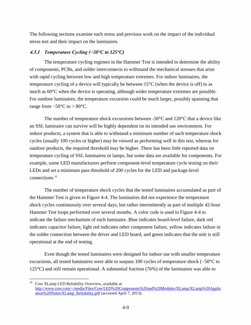
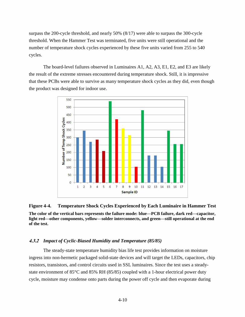
The number of temperature shock cycles that the tested luminaires accumulated as part of
the Hammer Test is given in Figure 4-4. The luminaires did not experience the temperature
shock cycles continuously over several days, but rather intermittently as part of multiple 42-hour
Hammer Test loops performed over several months. A color code is used in Figure 4-4 to
indicate the failure mechanism of each luminaire. Blue indicates board-level failure, dark red
indicates capacitor failure, light red indicates other component failure, yellow indicates failure in
the solder connection between the driver and LED board, and green indicates that the unit is still
operational at the end of testing.
Even though the tested luminaires were designed for indoor use with smaller temperature
excursions, all tested luminaires were able to surpass 100 cycles of temperature shock (−50°C to
125°C) and still remain operational. A substantial fraction (76%) of the luminaires was able to
10
Cree XLamp LED Reliability Overview, available at
http://www.cree.com/~/media/Files/Cree/LED%20Components%20and%20Modules/XLamp/XLamp%20Applic
ation%20Notes/XLamp_Reliability.pdf (accessed April 7, 2013).
4-10
surpass the 200-cycle threshold, and nearly 50% (8/17) were able to surpass the 300-cycle
threshold. When the Hammer Test was terminated, five units were still operational and the
number of temperature shock cycles experienced by these five units varied from 255 to 540
cycles.
The board-level failures observed in Luminaires A1, A2, A3, E1, E2, and E3 are likely
the result of the extreme stresses encountered during temperature shock. Still, it is impressive
that these PCBs were able to survive as many temperature shock cycles as they did, even though
the product was designed for indoor use.
Figure 4-4. Temperature Shock Cycles Experienced by Each Luminaire in Hammer Test
The color of the vertical bars represents the failure mode: blue—PCB failure, dark red—capacitor,
light red—other components, yellow—solder interconnects, and green—still operational at the end
of the test.
4.3.2 Impact of Cyclic-Biased Humidity and Temperature (85/85)
The steady-state temperature humidity bias life test provides information on moisture
ingress into non-hermetic packaged solid-state devices and will target the LEDs, capacitors, chip
resistors, transistors, and control circuits used in SSL luminaires. Since the test uses a steady-
state environment of 85°C and 85% RH (85/85) coupled with a 1-hour electrical power duty
cycle, moisture may condense onto parts during the power off cycle and then evaporate during
4-11
the power on cycle when the device warms up. This is especially likely to occur in devices such
as power transistors and LEDs, which handle sufficient currents to heat up relative to ambient.
However, this test differs slightly from the traditional extended humidity soak test since the
duration is only 6 hours and is followed by either temperature shock cycles of a high temperature
bake.
Extensive studies on LED performance in 85/85 have already been acquired by most
LED manufacturers, although the data are typically reported only in summary form.8 In addition,
most electronics manufacturers test electrical components and PCBs under conditions of cycling-
biased humidity. However, studies performed on lamps and luminaires under cyclic bias in
conditions of known temperature and humidity are rare. One study by RTI has shown that biased
cycling of SSL luminaires at 85/85 produces a number of impacts, including (1) accelerating the
rate of lumen depreciation of LEDs, especially warm white LEDs; (2) increasing light absorption
for some lenses, especially polycarbonate-based materials; and (3) accelerating the aging of paint
and reflector surfaces.11 All of these processes will increase the rate of lumen depreciation in the
luminaire system.
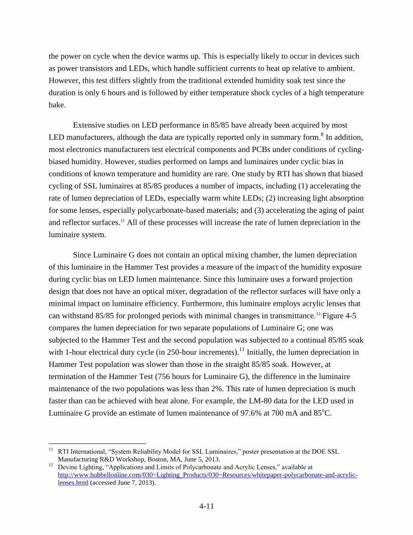
Since Luminaire G does not contain an optical mixing chamber, the lumen depreciation
of this luminaire in the Hammer Test provides a measure of the impact of the humidity exposure
during cyclic bias on LED lumen maintenance. Since this luminaire uses a forward projection
design that does not have an optical mixer, degradation of the reflector surfaces will have only a
minimal impact on luminaire efficiency. Furthermore, this luminaire employs acrylic lenses that
can withstand 85/85 for prolonged periods with minimal changes in transmittance.12 Figure 4-5
compares the lumen depreciation for two separate populations of Luminaire G; one was
subjected to the Hammer Test and the second population was subjected to a continual 85/85 soak
with 1-hour electrical duty cycle (in 250-hour increments).11
Initially, the lumen depreciation in
Hammer Test population was slower than those in the straight 85/85 soak. However, at
termination of the Hammer Test (756 hours for Luminaire G), the difference in the luminaire
maintenance of the two populations was less than 2%. This rate of lumen depreciation is much
faster than can be achieved with heat alone. For example, the LM-80 data for the LED used in
Luminaire G provide an estimate of lumen maintenance of 97.6% at 700 mA and 85oC.
11
RTI International, “System Reliability Model for SSL Luminaires,” poster presentation at the DOE SSL
Manufacturing R&D Workshop, Boston, MA, June 5, 2013. 12
Devine Lighting, “Applications and Limits of Polycarbonate and Acrylic Lenses,” available at
http://www.hubbellonline.com/030~Lighting_Products/030~Resources/whitepaper-polycarbonate-and-acrylic-
lenses.html (accessed June 7, 2013).
4-12
Figure 4-5. Comparison of the Change in Lumen Maintenance for Two Different
Populations of Luminaire G
The Hammer Test population was subjected to the conditions of the Hammer Test as described in
this report. The 85/85 only population was subjected to a continuous soak at 85/85 with a 1-hour
electrical duty cycle, and these results are reported elsewhere.11
For both populations, all
luminaires were still operational at 750 hours of testing.
4.3.3 Impact of High-Temperature Operational Lifetime (HTOL) Test (120oC)
The HTOL test is typically used to investigate the impact of temperature on accelerating
the degradation of parts under testing. In addition, the application of voltage to electrical
components at high temperature allows an investigation of the simultaneous impacts of
temperature and voltage on electrical components and solid-state devices over time. This test
simulates the device’s operating condition, but in an accelerated fashion that can provide insights
into the intrinsic reliability of electrical components. Since component degradation often occurs
through chemical processes (e.g., formation of intermetallics, materials aging, capacitor
electrolyte degradation), temperatures above the normal device operating temperature can have a
significant accelerating affect. In addition, non-electrical components of luminaires such as
plastics and reflectors often degrade via analogous chemical processes that would be accelerated
by temperature. However, the acceleration rates of various processes may differ, which must be
80
82
84
86
88
90
92
94
96
98
100
102
0 200 400 600 800
Lum
en
Mai
nte
nan
ce (%
)
Exposure Time (hours)
Comparison of Lumen Depreciation for Luminaire G
Hammer Test
85/85 Only
4-13
taken into account when examining data from HTOL experiments. When performed for a short
duration, the HTOL test is similar to a burn-in test that is often used to screen early failures.
A variety of high temperature (HT) and HTOL tests have been performed on components
of SSL luminaires, but only limited testing has been reported on SSL lamps and luminaires. In
one of the few publicly available datasets on HTOL testing of SSL lamps, DOE reported on
results from stress testing of the Philips 60W L Prize entry.13 In these tests, the SSL lamps were
subjected to ambient temperatures as high as 136.7°C with minimal impact on overall
performance. In exposing the luminaire to high temperatures, it is important to understand the
impact of the temperature on any plastic parts used in the luminaires. For the luminaire
assemblies tested in the Hammer Test, the plastics used in Luminaires A, B, C, and G were
compatible with the highest temperature (i.e., 125oC) used in the Hammer Test. Consequently,
these luminaires were tested as received in the Hammer Test, and findings on these devices apply
to the entire luminaire assembly. In contrast, the plastics used in Luminaires D, E, and F
distorted during the high temperature of the Hammer Test and had to be removed before testing.
As discussed above, these plastics were returned to the luminaire testing, allowing a
determination of the changes in the rest of the luminaire assembly (e.g., typically, the LEDs,
drivers, and associated interconnects).
The most common HTOL data available for SSL components used in luminaires are LM-
80 data, which will report LED operational characteristics often at temperatures up to 125°C.
Numerous other researchers have detailed the impacts of temperature on white LED components,
including GaN, phosphors, and epoxy encapsulants.14 Other components of the SSL luminaire
have not been studied as extensively under HT and HTOL, but several notable results have been
published. Han and Narendran examined the impact of temperatures as high as 180°C on LED
driver performance,15 and other researchers have focused on the impact of temperature on the
lifetime of electrolytic capacitors.16,17 A significant body of work also exists on the impact of
13
M.E. Poplawski, M.R. Ledbetter, and M.A. Smith, “Stress Testing of the Philips 60 W Replacement Lamp L-
Prize Entry,” PNNL-20391, April 2012. 14
W.D. van Driel and X.J. Fan, editors, Solid State Lighting Reliability: Components to Systems, Springer, New
York, NY, 2012. 15
L. Han and N. Narendran, “An Accelerated Test Method for Predicting the Useful Life of an LED Driver,” IEEE
Transactions on Power Electronics; August 2011; 26(8): 2249–2257. 16
H. Van der Broeck, G. Sauerlander, and M. Wendt, “Temperature Dependency in Performance of Solid-State
Lighting Drivers,” 2011, 12th International Conference of Thermal, Mechanical and Multiphysics Simulation
and Experiments in Microelectronics and Microsystems (EuroSimE 2011). 17
C.S. Kulkarni, J. Celaya, K. Goebel, and G. Biswas, “Physics-based Electrolytic Capacitor Degradation Models
for Prognostics under Thermal Overstress,” European Conference of the Prognostics and Health Management
Society (2012), p. 1.
4-14
temperature on solders, PCBs, and integrated circuits.18 All of this information may be useful in
understanding potential failure mechanisms in SSL luminaires, but there may be some system-
level effects that are unique to SSL luminaires.
4.4 LED Performance in the Hammer Test
A predictive finite element model (FEM) was developed for several of the luminaires
examined in the Hammer Test to understand the impact of high ambient temperatures on the
luminaire. In principle, the creation of a FEM model that matches a luminaire’s experimental
performance at operating conditions will allow consistent prediction of that luminaire’s thermal
performance under a broader range of operating conditions. Finding the LED junction
temperature (Tj) is generally of most interest. For Luminaire B, Tj was acquired through the
following process. First, a Solidworks model of the downlight was created, at the level of detail
thought appropriate to capture the important physical/thermal processes. Second, the Solidworks
files were imported to ANSYS (v 11), where a steady-state thermal model was created. This was
done by assigning material characteristics to the various components (specifically thermal
conductivity) and specifying boundary conditions such as volumetric heat production (at the
LED) and free convection or radiation (at the fins or other outside surfaces). Third, the model
was run and iterated to a self-consistent equilibrium, making sure to include items like the
temperature-voltage coefficient upon power dissipation and the appropriate thermal resistance
from junction to solder, information provided on the LED specification sheet. The final steady-
state temperature model predicted a Tj of between 38°C and 44°C, for an ambient temperature of
25°C, compared to a thermocouple-measured value of 49°C.
One of the critical questions that the Hammer Test is seeking to answer concerns the
robustness of luminaire components, principally LEDs and other electronic components. The
extreme conditions of the Hammer Test, in particular the high-temperature excursions, were
intended to overstress the LEDs by increasing the junction temperature to or above the LED
design limits. All of the LEDs used in the tested luminaires had junction -to-solder point
resistances (js) below 18°C/W. Assuming the power dissipation in HBLEDs is < 1.5 W (i.e.,
500 mA and 3 Volts), this would equate to a temperature difference between the LED junction
and the solder point of < 27°C. Therefore, the HBLED junction temperatures (Tj) at the highest
temperature used in the Hammer Test should be < 152°C, which is right at the specified
maximum junction temperature. A similar analysis for the MPLEDs (using 150 mA at 3 Volts)
reveals that the likely maximum Tj value is approximately 135°C, which is 10°C higher than the
18
P. Lall, M.G. Pecht, and E.B. Hakim, Influence of Temperature on Microelectronics and System Reliability,
1997, CRC Press, Boca Raton, Florida.
4-15
specified maximum Tj value for the LED used in Luminaire E, but below the maximum Tj value
for the LED used in Luminaire F.
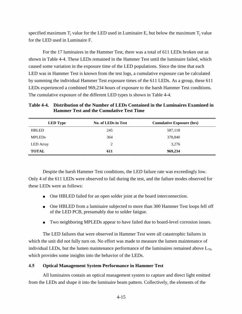
For the 17 luminaires in the Hammer Test, there was a total of 611 LEDs broken out as
shown in Table 4-4. These LEDs remained in the Hammer Test until the luminaire failed, which
caused some variation in the exposure time of the LED populations. Since the time that each
LED was in Hammer Test is known from the test logs, a cumulative exposure can be calculated
by summing the individual Hammer Test exposure times of the 611 LEDs. As a group, these 611
LEDs experienced a combined 969,234 hours of exposure to the harsh Hammer Test conditions.
The cumulative exposure of the different LED types is shown in Table 4-4.
Table 4-4. Distribution of the Number of LEDs Contained in the Luminaires Examined in
Hammer Test and the Cumulative Test Time
LED Type No. of LEDs in Test Cumulative Exposure (hrs)
HBLED 245 587,118
MPLEDs 364 378,840
LED Array 2 3,276
TOTAL 611 969,234
Despite the harsh Hammer Test conditions, the LED failure rate was exceedingly low.
Only 4 of the 611 LEDs were observed to fail during the test, and the failure modes observed for
these LEDs were as follows:
■ One HBLED failed for an open solder joint at the board interconnection.
■ One HBLED from a luminaire subjected to more than 300 Hammer Test loops fell off
of the LED PCB, presumably due to solder fatigue.
■ Two neighboring MPLEDs appear to have failed due to board-level corrosion issues.
The LED failures that were observed in Hammer Test were all catastrophic failures in
which the unit did not fully turn on. No effort was made to measure the lumen maintenance of
individual LEDs, but the lumen maintenance performance of the luminaires remained above L70,
which provides some insights into the behavior of the LEDs.
4.5 Optical Management System Performance in Hammer Test
All luminaires contain an optical management system to capture and direct light emitted
from the LEDs and shape it into the luminaire beam pattern. Collectively, the elements of the
4-16
optical management system comprise the housing and structure of the luminaire. Examples of
materials that light may encounter in the luminaire optical management system include the
following:
■ Solder masks
■ Other LEDs and components (e.g., diodes and transistors)
■ Reflector surfaces
■ Diffusers
■ Lenses.
Table 3-1 provides information on the type of reflectors, lenses, and number of LEDs that
are contained in each luminaire’s optical cavity. As light interacts with each of these elements, it
can be adsorbed, transmitted, or reflected. During aging, the relative ratios of absorbance,
transmittance, and reflectance may change, which would alter the luminous flux produced by the
luminaire. An increase in absorbance by the optical management systems components can
significantly reduce luminous flux produced by SSL luminaires. In addition, if the absorbance
change varies across the spectrum (e.g., blue absorbance changes more than red), a color shift
may occur. The performance of common materials used in optical management systems for
downlights has been discussed previously.19 In general, material chemistry, temperature,
environment, and blue photon flux all impact the aging of optical management system
components.
The impact of changes in the optical management system on the luminous flux emitted
from the SSL luminaire is also dependent on luminaire design. For example, downlights with
appreciable optical mixing chambers would be more sensitive to changes in reflector surfaces
than those without mixing chambers. Table 3-1 provides insights into the use of optical mixing
cavities in each luminaire examined in the Hammer Test. In designing a luminaire, designers
take into consideration the tradeoffs between diffusion of the light emitted by the LEDs, desired
beam pattern, and intended mounting structure. In addition, there are several ways to diffuse the
light emitted by each LED, including optical mixing chambers, diffusing films, and diffusing
lenses. Consequently, a variety of luminaire designs incorporating different optical management
system designs are in use, as reflected in Table 3-1.
19
J. Lynn Davis, M. Lamvik, J. Bittle, S. Shepherd, R. Yaga, N. Baldasaro, E. Solano, and G. Bobashev. Insights
into accelerated aging of SSL luminaires. Proceedings of SPIE, Volume 8835 (2013).
4-17
In all of the luminaires examined in the Hammer Test, all light radiating from the
luminaire must pass through a diffuser and lens. In some instances, these two elements are
combined into a single diffuser lens. Consequently changes in lens absorbance significantly
impact the luminous flux from the luminaire. The plastics used in Luminaires D, E, and F were
not compatible with the high temperature used in the bake cycle of the Hammer Test. As a result,
these plastics had to be removed during the Hammer Test cycle, but were replaced on the
luminaire prior to integrated sphere measurements. So no information on the impact of Hammer
Test on the lenses used in these luminaires could by obtained.
In contrast, the plastics used in Luminaires A, B, C, and G have glass transition
temperatures well above the upper test limit of the Hammer Test, so these luminaires could
remain intact during testing. The material used in these optical elements consisted of acrylics and
polycarbonates. Both polymers have certain advantages and disadvantages as explained
elsewhere, 20 so the choice of material is dependent on the product design.
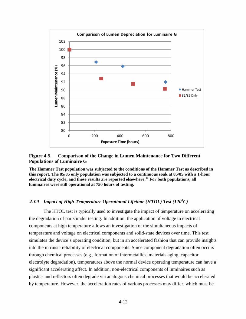
In general, the absorbance of polycarbonate materials was found to increase during the
Hammer Test, while that of acrylates changed little. The absorbance increase for polycarbonates
occurs initially in the blue region of the spectrum, but can gradually spread to other wavelengths
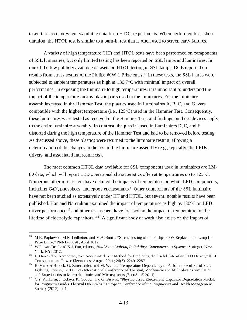
with additional exposure. For example, the change in absorbance for a lens subjected to the
Hammer Test is shown in Figure 4-6, and a similar measurement for the diffuser films used in
several of the luminaires is shown in Figure 4-7. The observed increase in blue absorbance is
fairly typical of polymer oxidation.21 For many polymers, oxidation results in increased
absorbance in the blue region of the spectrum, which is often manifested as a yellowing of the
polymer. Since blue light has a relatively low lumen content, the overall impact on luminous flux
may be small for low levels of oxidation, but can increase significantly for more highly oxidized
polymers.19
In addition, the increased filtering of blue light can produce a color shift in the
luminaire, even with low levels of polymer oxidation.
The color shift of the luminaires in the Hammer Test will depend on the changes in the
LEDs and the optical management system used. As noted above, both of these parameters are
impacted by the length of Hammer Test exposure. To provide a common basis for comparing
color shifts observed in the luminaires, the u’v’ values after 10 loops (i.e., 420 hours) are given
in this report. Luminaires D and G exhibited the smallest shift, with a u’v’ value of 0.0004. The
20
Devine Lighting, “Applications and Limits of Polycarbonate and Acrylic Lenses,” available at
http://www.hubbellonline.com/030~Lighting_Products/030~Resources/whitepaper-polycarbonate-and-acrylic-
lenses.html (accessed June 7, 2013). 21
K. Pielichowski and J. Njuguna, Thermal Degradation of Polymeric Materials, (2005) RAPRA Technology,
Shawbury, United Kingdom.
4-18
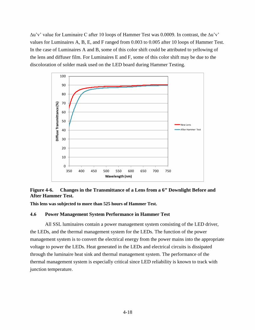
u’v’ value for Luminaire C after 10 loops of Hammer Test was 0.0009. In contrast, the u’v’
values for Luminaires A, B, E, and F ranged from 0.003 to 0.005 after 10 loops of Hammer Test.
In the case of Luminaires A and B, some of this color shift could be attributed to yellowing of
the lens and diffuser film. For Luminaires E and F, some of this color shift may be due to the
discoloration of solder mask used on the LED board during Hammer Testing.
Figure 4-6. Changes in the Transmittance of a Lens from a 6″ Downlight Before and
After Hammer Test.
This lens was subjected to more than 525 hours of Hammer Test.
4.6 Power Management System Performance in Hammer Test
All SSL luminaires contain a power management system consisting of the LED driver,
the LEDs, and the thermal management system for the LEDs. The function of the power
management system is to convert the electrical energy from the power mains into the appropriate
voltage to power the LEDs. Heat generated in the LEDs and electrical circuits is dissipated
through the luminaire heat sink and thermal management system. The performance of the
thermal management system is especially critical since LED reliability is known to track with
junction temperature.
0
10
20
30
40
50
60
70
80
90
100
350 400 450 500 550 600 650 700 750
Dif
fuse
Tra
nsm
itta
nce
(%)
Wavelength (nm)
New Lens
After Hammer Test
4-19
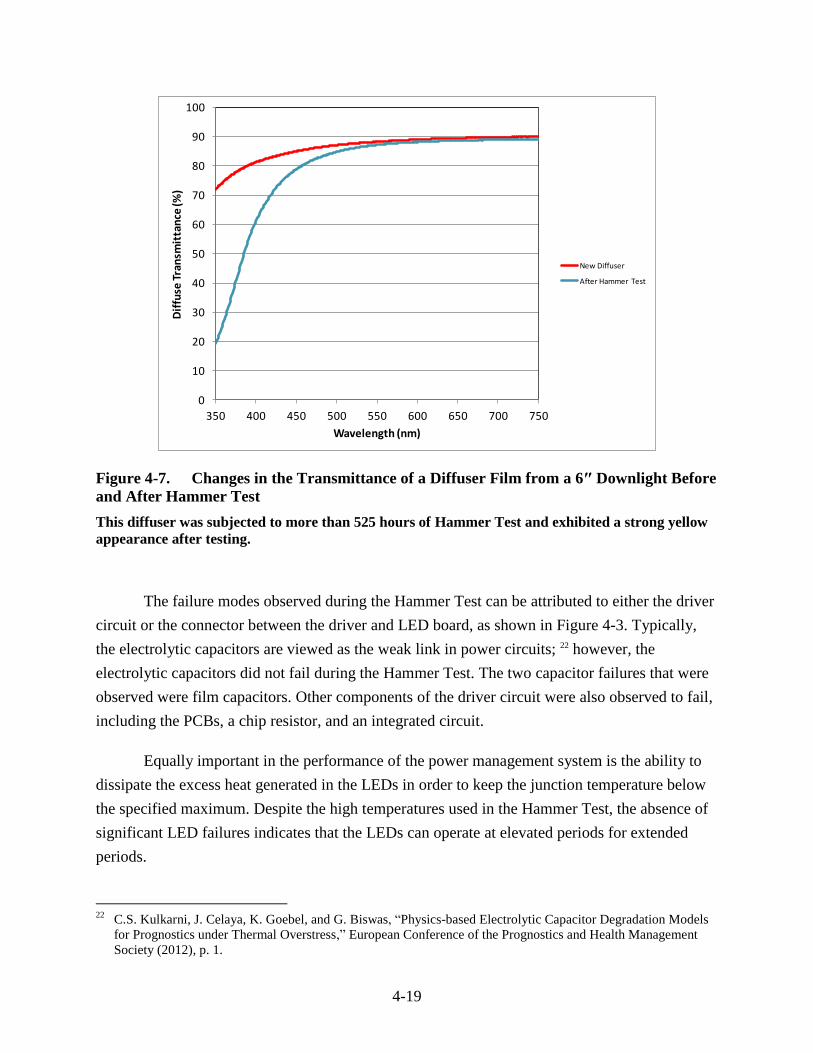
Figure 4-7. Changes in the Transmittance of a Diffuser Film from a 6″ Downlight Before
and After Hammer Test
This diffuser was subjected to more than 525 hours of Hammer Test and exhibited a strong yellow
appearance after testing.
The failure modes observed during the Hammer Test can be attributed to either the driver
circuit or the connector between the driver and LED board, as shown in Figure 4-3. Typically,
the electrolytic capacitors are viewed as the weak link in power circuits; 22 however, the
electrolytic capacitors did not fail during the Hammer Test. The two capacitor failures that were
observed were film capacitors. Other components of the driver circuit were also observed to fail,
including the PCBs, a chip resistor, and an integrated circuit.
Equally important in the performance of the power management system is the ability to
dissipate the excess heat generated in the LEDs in order to keep the junction temperature below
the specified maximum. Despite the high temperatures used in the Hammer Test, the absence of
significant LED failures indicates that the LEDs can operate at elevated periods for extended
periods.
22
C.S. Kulkarni, J. Celaya, K. Goebel, and G. Biswas, “Physics-based Electrolytic Capacitor Degradation Models
for Prognostics under Thermal Overstress,” European Conference of the Prognostics and Health Management
Society (2012), p. 1.
0
10
20
30
40
50
60
70
80
90
100
350 400 450 500 550 600 650 700 750
Dif
fuse
Tra
nsm
itta
nce
(%)
Wavelength (nm)
New Diffuser
After Hammer Test
5-1
SECTION 5
CONCLUSIONS
To accommodate the rapid evolution of SSL technologies and fully realize their energy
savings potential, there is a widespread need in the lighting industry to understand potential
failure modes of luminaires. However, failure modes of lamps and luminaires are not often
reported. In one effort, the robustness of fluorescent lamps and the Philips L-Prize lamp were
compared using a series of step stress experiments varying temperature cycling, vibration, and
voltage.13
In these tests, all of the fluorescent lamps failed during the step stress experiments,
whereas no failures of the L-Prize lamps could be produced within the same stress envelope.
This finding demonstrates the potential robustness of LED lighting systems.
In the Hammer Test studies described in this report, entire SSL luminaires were subjected
to extreme environmental stressors, including temperature cycling, temperature and humidity
soak, and high temperature bake. Electrical power was cycled to the luminaires during testing
providing electrical stress as well. All of the luminaires examined during the Hammer Test were
designed for indoor use and not expected to encounter environmental extremes. However, this
study demonstrated that such SSL luminaires can exhibit exceptional durability even under the
extreme stresses of the Hammer Test. All luminaires examined in this study survived more than
100 cycles of temperature shock (–50°C to 125°C) and nearly half survived more than 300
cycles. The failures that were observed typically occurred in the driver circuit, with board-level
failures being most common. The 611 LEDs in these luminaires endured nearly 1 million hours
of cumulative exposure to the Hammer Test with only four failures. Two of these LED failures
were attributed to solder joint fatigue and the other two failures were due to board-level
corrosion. These findings reinforce the high reliability of LEDs in lighting systems, even under
extreme conditions, and suggests that other elements of the luminaire are more likely to fail first.
Consequently, a systems-level perspective, including LEDs, drivers, optics, and other
components, need to be considered when evaluating the long term performance of SSL
luminaires.
In conclusion, SSL luminaires are robust and can withstand the extreme stresses of the
Hammer Test. The level of performance demonstrated by the luminaires examined in this
Hammer Test protocol suggests that SSL luminaires will have a low probability of random
failure in the field during normal use, and that properly designed and installed SSL luminaires
are likely to have long lifetimes under normal operating conditions. However, additional work is
needed to determine actual wear-out mechanisms, quantify failure modes, and determine
5-2
acceleration factors for SSL luminaires. This information is necessary in order to provide
estimates of lifetime and reliability.
5-3
APPENDIX
Estimating Acceleration Factors for the Hammer Test1
The acceleration factor (AF) of an accelerated life test (ALT) is a dimensionless value
that relates the lifetime observed for a product in a specific ALT to that of the expected lifetime
of an equivalent product under normal (i.e., non-accelerated) operating conditions. In its most
basic form the acceleration factor is given by:
The AF value will depend upon a number of parameters, including
■ Test settings during ALT (.e.g., temperature, humidity, etc.)
■ Environmental conditions during normal operation
■ Failure mode being accelerated.
The luminaires examined during the Hammer Test are intended for indoor use and will
typically experience environments where the ambient temperature is between 20°C and 30°C and
the ambient relative humidity is between 30% and 60%. These conditions are significantly
different from those of the Hammer Test, as discussed in Section 2 of the main report. Further,
the Hammer Test consists of three different ALTs:
■ Steady-state temperature humidity biased life test
■ Temperature shock life test
■ High temperature operations lifetime (HTOL) test.
As will be demonstrated below, the AF value of each of the tests used in the Hammer
Test is likely to be different. Further, it is important to have an understanding of the failure
modes occurring during ALT in order to properly calculate the AF of each phase of the Hammer
Test. As demonstrated in Figure 4-3 of the main report, there are multiple failure modes
observed during the testing, making the assignment of a universal AF value difficult. However,
some estimates of the AF values can be calculated using standard procedures and will be
discussed below.
1 This section was written in close consultation with Willem van Driel of Philips.
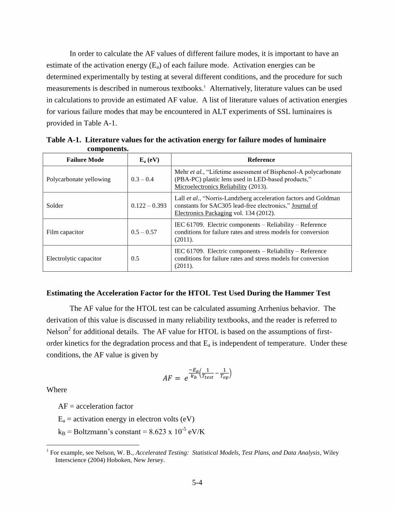
5-4
In order to calculate the AF values of different failure modes, it is important to have an
estimate of the activation energy (Ea) of each failure mode. Activation energies can be
determined experimentally by testing at several different conditions, and the procedure for such
measurements is described in numerous textbooks.1 Alternatively, literature values can be used
in calculations to provide an estimated AF value. A list of literature values of activation energies
for various failure modes that may be encountered in ALT experiments of SSL luminaires is
provided in Table A-1.
Table A-1. Literature values for the activation energy for failure modes of luminaire
components.
Failure Mode Ea (eV) Reference
Polycarbonate yellowing 0.3 – 0.4
Mehr et al., “Lifetime assessment of Bisphenol-A polycarbonate
(PBA-PC) plastic lens used in LED-based products,”
Microelectronics Reliability (2013).
Solder 0.122 – 0.393
Lall et al., “Norris-Landzberg acceleration factors and Goldman
constants for SAC305 lead-free electronics,” Journal of
Electronics Packaging vol. 134 (2012).
Film capacitor 0.5 – 0.57
IEC 61709. Electric components – Reliability – Reference
conditions for failure rates and stress models for conversion
(2011).
Electrolytic capacitor 0.5
IEC 61709. Electric components – Reliability – Reference
conditions for failure rates and stress models for conversion
(2011).
Estimating the Acceleration Factor for the HTOL Test Used During the Hammer Test
The AF value for the HTOL test can be calculated assuming Arrhenius behavior. The
derivation of this value is discussed in many reliability textbooks, and the reader is referred to
Nelson2 for additional details. The AF value for HTOL is based on the assumptions of first-
order kinetics for the degradation process and that Ea is independent of temperature. Under these
conditions, the AF value is given by
Where
AF = acceleration factor
Ea = activation energy in electron volts (eV)
kB = Boltzmann’s constant = 8.623 x 10⁻⁵
eV/K
1 For example, see Nelson, W. B., Accelerated Testing: Statistical Models, Test Plans, and Data Analysis, Wiley
Interscience (2004) Hoboken, New Jersey.
5-5
Ttest = temperature in test environment (in K)
Top = temperature in normal operating environment (in K)
As an example, assume the failure mode of a material has an Ea value of 0.4 eV and that
its temperature during normal operation is 25°C. Accelerating the degradation of the material by
rising its temperature to 120°C produces an acceleration factor of 43. This means that if the
materials lasted for 1,000 hours during the ALT, then it can be expected to last for 43,000 hours
under normal operating conditions. Of course, the same definition of failure must be used in
both cases.
Estimating the Acceleration Factor for the Steady-State Temperature Humidity Biased
Lifetime Test
Peck1 examined the impact of temperature and humidity upon the lifetime of epoxy
encapsulated integrated circuits, and created a formula for calculating the AF value for tests such
as 85/85. The Peck relationship for calculating the temperature-humidity acceleration is:
Where
AF = acceleration factor
RHop = relative humidity in the normal operating environment (in %)
RHtest = relative humidity in the test environment (in %)
n = a constant determined through testing (typical values are between 2 and 3)
Ea = activation energy in eV
kB = Boltzmann’s constant = 8.623 x 10⁻⁵
eV/K
Ttest = temperature in test environment (in K)
Top = temperature in normal operating environment (in K)
The yellowing of polycarbonate lenses used in SSL luminaires is accelerated by
temperature and humidity and can produce lumen depreciation.2
Assume that the normal
operating environment of a polycarbonate lens is 25°C and 40% RH and that the activation
energy for this chemical process is 0.333 eV. Then the AF value in 85/85 can be calculated to be
39, assuming a conservative value of n = 2.
1 Peck, “Comprehensive model for humidity testing correlation,” 24th Annual Reliability Physics Symposium
(1986) 44. 2 Davis, J.L. et al., “Insights into accelerated aging of SSL luminaires,” Proceedings of the SPIE 8835 (2013)
883502-1.
5-6
For simplicity, the temperature and RH value of the lens are assumed to be the same as
the ambient environment. During operation, the lens will typically heat up by 20-30°C, which
will also impact the RH value. Either thermal models or spot temperature measurements are
necessary to provide more accurate estimates of the acceleration factor.
Estimating the Acceleration Factor for the Temperature Shock Test Used During Hammer
Test
Temperature shock testing is typically performed on assemblies to investigate the impact
of expansion and contraction. The temperature shock test imparts several environmental stresses
on the assembly, including high temperature, low temperature, and the frequency of changing
between the two. There are several different formalisms that have been developed for
calculating acceleration factors of temperature shock experiments, with the Coffin-Manson and
Norris-Landzberg modification being the most commonly used. For this analysis, the Norris-
Landzberg modification of the Coffin-Manson equation will be used. This equation is:
Where
AF = acceleration factor
Ttest = the difference between the high and low temperatures during testing
Top = the difference between the high and low temperatures during normal operation
n = a constant with a typical value of 1.9 – 2.0.
fop = is the cycling frequency during normal operation (in cycles per day)
ftest = is the cycling frequency during the temperature shock test (in cycles per day)
m = a constant with a typical value of 0.33
Ea = activation energy in eV
kB = Boltzmann’s constant = 8.623 x 10⁻⁵
eV/K
Ttest,max = maximum temperature in test environment (in K)
Top,max = maximum temperature in normal operating environment (in K)
During normal operation, the solder joints on SSL luminaires will experience heating and
cooling cycles as the luminaire is turned on and off. Assume that the temperature of the solder
joints is 25°C when off and 65°C when the unit is on and that the unit is turned on and off twice
a day (i.e.., fop = 2). During the temperature shock test, assume that the temperature of the solder
joints is in equilibrium with the ambient temperature, so Ttest = 175°C and the cycling
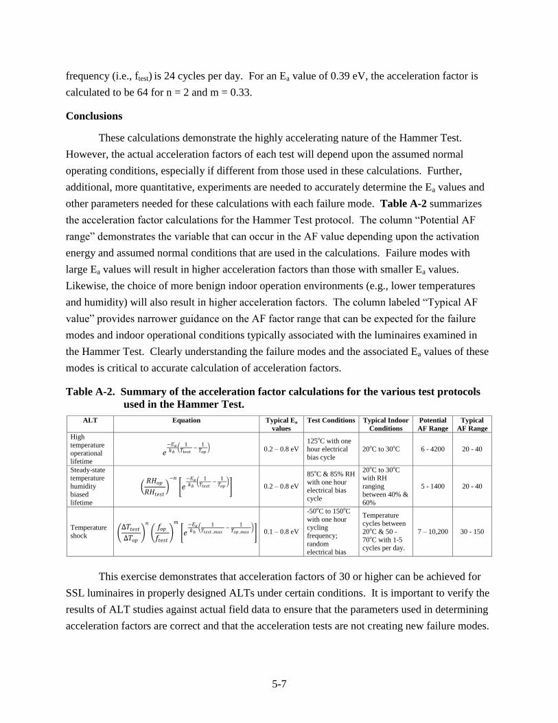
5-7
frequency (i.e., ftest) is 24 cycles per day. For an Ea value of 0.39 eV, the acceleration factor is
calculated to be 64 for n = 2 and m = 0.33.
Conclusions
These calculations demonstrate the highly accelerating nature of the Hammer Test.
However, the actual acceleration factors of each test will depend upon the assumed normal
operating conditions, especially if different from those used in these calculations. Further,
additional, more quantitative, experiments are needed to accurately determine the Ea values and
other parameters needed for these calculations with each failure mode. Table A-2 summarizes
the acceleration factor calculations for the Hammer Test protocol. The column “Potential AF
range” demonstrates the variable that can occur in the AF value depending upon the activation
energy and assumed normal conditions that are used in the calculations. Failure modes with
large Ea values will result in higher acceleration factors than those with smaller Ea values.
Likewise, the choice of more benign indoor operation environments (e.g., lower temperatures
and humidity) will also result in higher acceleration factors. The column labeled “Typical AF
value” provides narrower guidance on the AF factor range that can be expected for the failure
modes and indoor operational conditions typically associated with the luminaires examined in
the Hammer Test. Clearly understanding the failure modes and the associated Ea values of these
modes is critical to accurate calculation of acceleration factors.
Table A-2. Summary of the acceleration factor calculations for the various test protocols
used in the Hammer Test.
This exercise demonstrates that acceleration factors of 30 or higher can be achieved for
SSL luminaires in properly designed ALTs under certain conditions. It is important to verify the
results of ALT studies against actual field data to ensure that the parameters used in determining
acceleration factors are correct and that the acceleration tests are not creating new failure modes.
ALT Equation
Typical Ea
values
Test Conditions Typical Indoor
Conditions
Potential
AF Range
Typical
AF Range
High
temperature
operational
lifetime
− 𝑘
1
−
1
0.2 – 0.8 eV
125oC with one
hour electrical
bias cycle
20oC to 30
oC 6 - 4200 20 - 40
Steady-state
temperature
humidity
biased
lifetime
−
− 𝑘
1
−
1
0.2 – 0.8 eV
85oC & 85% RH
with one hour
electrical bias
cycle
20oC to 30
oC
with RH
ranging
between 40% &
60%
5 - 1400 20 - 40
Temperature
shock
− 𝑘
1
, −
1 ,
0.1 – 0.8 eV
-50oC to 150
oC
with one hour
cycling
frequency;
random
electrical bias
Temperature
cycles between
20oC & 50 -
70oC with 1-5
cycles per day.
7 – 10,200 30 - 150
5-8
If these guidelines are followed, ALTs can be performed in a manner that reduces testing time
and provides accurate insights into expected lifetimes and failure modes of SSL luminaires.