Hakula, Harri; Quach, Tri; Rasila, Antti The Conjugate ...

This is an electronic reprint of the original article.This reprint may differ from the original in pagination and typographic detail.

Powered by TCPDF (www.tcpdf.org)

This material is protected by copyright and other intellectual property rights, and duplication or sale of all or part of any of the repository collections is not permitted, except that material may be duplicated by you for your research use or educational purposes in electronic or print form. You must obtain permission for any other use. Electronic or print copies may not be offered, whether for sale or otherwise to anyone who is not an authorised user.

Hakula, Harri; Quach, Tri; Rasila, AnttiThe Conjugate Function Method and Conformal Mappings in Multiply Connected Domains

Published in:SIAM Journal on Scientific Computing

DOI:10.1137/17M1124164

Published: 01/01/2019

Document VersionPublisher's PDF, also known as Version of record

Please cite the original version:Hakula, H., Quach, T., & Rasila, A. (2019). The Conjugate Function Method and Conformal Mappings in MultiplyConnected Domains. SIAM Journal on Scientific Computing, 41(3), A1753-A1776.https://doi.org/10.1137/17M1124164

https://doi.org/10.1137/17M1124164

https://doi.org/10.1137/17M1124164

Copyright © by SIAM. Unauthorized reproduction of this article is prohibited.

SIAM J. SCI. COMPUT. c\bigcirc 2019 Society for Industrial and Applied MathematicsVol. 41, No. 3, pp. A1753--A1776

THE CONJUGATE FUNCTION METHOD AND CONFORMALMAPPINGS IN MULTIPLY CONNECTED DOMAINS\ast

HARRI HAKULA\dagger , TRI QUACH\dagger , AND ANTTI RASILA\ddagger

Abstract. The conjugate function method is an algorithm for numerical computation of con-formal mappings for simply and doubly connected domains. In this paper the conjugate functionmethod is generalized for multiply connected domains. The key challenge addressed here is the con-struction of the conjugate domain and the associated conjugate problem. All variants of the methodpreserve the so-called reciprocal relation of the moduli. An implementation of the algorithm is givenalong with several examples and illustrations.

Key words. numerical conformal mappings, conformal modulus, multiply connected domains,canonical domains

AMS subject classifications. 30C30, 65E05, 31A15, 30C85

DOI. 10.1137/17M1124164

1. Introduction. Conformal mappings play an important role in theoreticalcomplex analysis and in certain engineering applications, such as electrostatics, aero-dynamics, and fluid mechanics. Existence of conformal mappings of simply connecteddomains onto the upper half-plane or the unit disk follows from the Riemann map-ping theorem, and there are generalizations of this result for doubly and multiplyconnected domains [2]. However, constructing such mappings analytically is usuallyvery difficult, and numerical methods are required.

There exists an extensive literature on numerical construction of conformal map-pings for simply and doubly connected domains [26]. One popular method is basedon the Schwarz--Christoffel formula [13], and its implementation SC Toolbox is dueto Driscoll [11, 12]. SC Toolbox itself is based on an earlier FORTRAN package byTrefethen [29]. A new algorithm involving a finite element method and the harmonicconjugate function was presented by the authors in [15].

While the study of numerical conformal mappings in multiply connected do-mains dates back to the 1980s [24, 27], recently there has been significant interestin the subject. DeLillo, Elcrat, and Pfaltzgraff [9] were the first to give a Schwarz--Christoffel formula for unbounded multiply connected domains. Their method relieson the Schwarzian reflection principle. Crowdy [4] was the first to derive a Schwarz--Christoffel formula for bounded multiply connected domains, which was based on theuse of the Schottky--Klein prime function. In a very recent paper [28] conformal mapsfrom multiply connected domains onto lemniscatic domains have been discussed. Thenatural extension of this result to unbounded multiply connected domains is given in[5]. It should be noted that a MATLAB implementation of the Schottky--Klein primefunction is freely available [7], and the algorithm is described in [8]. A method involv-ing the harmonic conjugate function is given in [23], but the approach there differs

\ast Submitted to the journal's Methods and Algorithms for Scientific Computing section April 4,2017; accepted for publication (in revised form) February 21, 2019; published electronically May 23,2019.

http://www.siam.org/journals/sisc/41-3/M112416.html\dagger Institute of Mathematics, Aalto University, FI-00076 Aalto, Finland ([email protected],

[email protected]).\ddagger Guangdong Technion -- Israel Institute of Technology, College of Science, Shantou, Guangdong

515063, China ([email protected], [email protected]).

A1753

Dow

nloa

ded

08/1

2/19

to 1

30.2

33.2

16.1

45. R

edis

trib

utio

n su

bjec

t to

SIA

M li

cens

e or

cop

yrig

ht; s

ee h

ttp://

ww

w.s

iam

.org

/jour

nals

/ojs

a.ph

p

http://www.siam.org/journals/sisc/41-3/M112416.html

mailto:[email protected]





A1754 HARRI HAKULA, TRI QUACH, AND ANTTI RASILA

from ours. Still another approach is given by Zeng and et al. [32], where Koebe'sconventional method for multiply connected planar surfaces is generalized.

The foundation of conjugate function methods for simply and doubly connecteddomains lies on properties of the (conformal) modulus, which originates from the the-ory of quasiconformal mappings [1, 22, 26]. Here we investigate conformal mappingsonto two types of canonical domains, and the associated boundary value problemsthat are, respectively, intended to generalize the concepts of the canonical quadrilat-eral and the ring domain, conformal mappings of which were investigated in [15]. Inthe following, for convenience we refer to these two classes of problems as Q-type andR-type, respectively.

Heuristically, the Q-type configuration refers to the situation where the ideal fluidflows from one arc on the exterior component of the boundary to another, and theinterior components of the boundary are understood as nonabsorbing. In this case,the canonical domain is a rectangle where the width is normalized to be one, theheight is a number d > 0 that can be understood as the modulus of the curve familyconnecting the above-mentioned boundary arcs, and the interior components of theboundary are mapped onto horizontal slits. The R-type configurations generalize theconcept of the ring domain, where ideal fluid flows from interior boundary componentsto the exterior boundary. In this case, the canonical domain is the spherical annulusAlogR = \{ z : 1 < | z| < R\} with radial slits. For simplicity, we investigate onlythe case of a Denjoy domain, where the canonical domain can be chosen so that theboundary components map onto line segments on the positive real axis. In particular,this is true for all triply connected domains (cf. [14, pp. 128--130]).

In terms of partial differential equations (PDEs), the conformal mapping is definedby a harmonic potential u and its harmonic conjugate v. One has to first find thepotential u by solving the Laplace equation \Delta u = 0 in the domain \Omega , with boundaryconditions

(1.1) 1N\partial u

\partial n+ 1Du = f(x, y) on \partial \Omega ,

where the indicator functions refer to Neumann and Dirichlet boundary parts, respec-tively. These boundary conditions can be defined by the application, thus determiningthe type of the problem, or alternatively the choice of the preferred mapping deter-mines the boundary conditions. In the cases considered here, from the solution u onecan formulate a conjugate problem with a solution v, the harmonic conjugate of u,and together u and v define the conformal mapping. Crucially, when the conjugateproblem is formulated, it is possible that cuts are introduced into the domain, andtherefore the computational domain is not necessarily the same in both solution steps.

Our two classes of problems are not exhaustive; however, the fundamental ideaspresented here can be applied to configurations not directly addressed by this paper.In Figure 1.1 two representative mappings of the same domain are constructed. Inboth cases the canonical domains are slit domains, first catalogued by Koebe [21].

Our method is suitable for a very general class of domains, allowing curved bound-aries and even cusps. The implementation of the algorithm is based on the hp-finiteelement method (hp-FEM) described in [16], and in [17] it is generalized to cover un-bounded domains. In [18], the method has been used to compute moduli of domainswith strong singularities.

The accuracy of the method has been evaluated by solving three benchmarkproblems: one computing resistances [10] and two on capacities [3]. In each case theresults agree with those obtained with either special-purpose methods or adaptiveh-FEM.

Dow

nloa

ded

08/1

2/19

to 1

30.2

33.2

16.1

45. R

edis

trib

utio

n su

bjec

t to

SIA

M li

cens

e or

cop

yrig

ht; s

ee h

ttp://

ww

w.s

iam

.org

/jour

nals

/ojs

a.ph

p


CONJUGATE FUNCTION METHOD AND CONFORMAL MAPPINGS A1755

(a) R-type. Contour plot of u.Dirichlet on all boundaries. Inte-rior u = 1, exterior u = 0. Saddlepoint and cuts are indicated.

(b) Q-type. Contour plot of u.Dirichlet on left (u = 0) andright (u = 1). Neumann zero-condition on other boundaries.Locations of maxima and minimaon the interior boundaries are in-dicated.

(c) R-type. Contour plot of u andv. Cuts are equipotential lines inv.

(d) Q-type. Contour plot of uand v.

0 1

d

3d/4

d/4

(e) R-type. Canonical domain in(u, v). Image scaled to d = 1.Saddle point lies on two orientedcuts. Width of the slit is deter-mined by the potential of u at thesaddle point. This domain can befurther mapped to annulus Ad.

0 1

d

d/2

(f) Q-type. Canonical domain in(u, v). Image scaled to d = 1.Width of the slit is determinedby the potential difference of uat the local maximum and min-imum.

Fig. 1.1. Conjugate function method and conformal mappings: Two circles in rectangle.

The rest of the paper is organized as follows. In section 2 the necessary conceptsfrom function theory are introduced. The new algorithms for multiply connecteddomains are described in sections 3 and 4 for types of R and Q, respectively. Afterthe numerical implementation is discussed, an extensive set of numerical experimentsis analyzed before brief conclusions are given.

2. Preliminaries. In this section we introduce concepts from function theoryand review the algorithm for simply or doubly connected domains. For details andreferences, see [15].

Dow

nloa

ded

08/1

2/19

to 1

30.2

33.2

16.1

45. R

edis

trib

utio

n su

bjec

t to

SIA

M li

cens

e or

cop

yrig

ht; s

ee h

ttp://

ww

w.s

iam

.org

/jour

nals

/ojs

a.ph

p



Definition 2.1 (modulus of a quadrilateral). A Jordan domain \Omega in \BbbC withmarked (positively ordered) points z1, z2, z3, z4 \in \partial \Omega is called a quadrilateral and de-noted by Q = (\Omega ; z1, z2, z3, z4). Then there is a canonical conformal map of the quadri-lateral Q onto a rectangle Rd = (\Omega \prime ; 1+ id, id, 0, 1), with the vertices corresponding towhere the quantity d defines the modulus of a quadrilateral Q. We write

M(Q) = d.

Notice that the modulus d is unique.

Lemma 2.2 (reciprocal identity). The reciprocal identity

(2.1) M(Q)M( \~Q) = 1

holds, where \~Q = (\Omega ; z2, z3, z4, z1) is called the conjugate quadrilateral of Q.

2.1. Dirichlet--Neumann problem. It is well known that one can express themodulus of a quadrilateral Q in terms of the solution of the Dirichlet--Neumann mixedboundary value problem.

Let \Omega be a domain in the complex plane whose boundary \partial \Omega consists of a finitenumber of piecewise regular Jordan curves, so that at every point, except possibly atfinitely many points of the boundary, an exterior normal is defined. Let \partial \Omega = A\cup B,where both A,B are unions of regular Jordan arcs such that A \cap B is finite. Let \psi A,\psi B be real-valued continuous functions defined on A,B, respectively. Find a functionu satisfying the following conditions:

1. u is continuous and differentiable in \Omega .2. u(t) = \psi A(t) for all t \in A.3. If \partial /\partial n denotes differentiation in the direction of the exterior normal, then

\partial

\partial nu(t) = \psi B(t) for all t \in B.

The problem associated with the conjugate quadrilateral \~Q is called the conjugateDirichlet--Neumann problem.

Let \gamma j , j = 1, 2, 3, 4, be the arcs of \partial \Omega between (z1, z2), (z2, z3), (z3, z4), (z4, z1),respectively. Suppose that u is the (unique) harmonic solution of the Dirichlet--Neumann problem with mixed boundary values of u equal to 0 on \gamma 2 and to 1 on\gamma 4, and \partial u/\partial n = 0 on \gamma 1, \gamma 3. Then

(2.2) M(Q) =

\int \int \Omega

| \nabla u| 2 dx dy.

Suppose that Q is a quadrilateral and u is the harmonic solution of the Dirichlet--Neumann problem, and let v be a conjugate harmonic function of u, v(Re z3, Im z3) = 0.Then f = u+ iv is an analytic function, and it maps \Omega onto a rectangle Rh such thatthe images of the points z1, z2, z3, z4 are 1 + id, id, 0, 1, respectively. Furthermore,by Carath\'eodory's theorem, f has a continuous boundary extension which maps theboundary curves \gamma 1, \gamma 2, \gamma 3, \gamma 4 onto the line segments \gamma \prime 1, \gamma

\prime 2, \gamma

\prime 3, \gamma

\prime 4.

Lemma 2.3. Let Q be a quadrilateral with modulus d, and let u be the harmonicsolution of the Dirichlet--Neumann problem. Suppose that v is the harmonic conjugatefunction of u, with v(Re z3, Im z3) = 0. If \~u is the harmonic solution of the Dirichlet--Neumann problem associated with the conjugate quadrilateral \~Q, then v = d\~u.

Dow

nloa

ded

08/1

2/19

to 1

30.2

33.2

16.1

45. R

edis

trib

utio

n su

bjec

t to

SIA

M li

cens

e or

cop

yrig

ht; s

ee h

ttp://

ww

w.s

iam

.org

/jour

nals

/ojs

a.ph

p



2.2. Ring domains. Let E0 and E1 be two disjoint and connected compact setsin the extended complex plane \BbbC \infty = \BbbC \cup \{ \infty \} . Then one of the sets E0 or E1 isbounded, and without loss of generality we may assume that it is E1. Then a setR = \BbbC \infty \setminus (E0 \cup E1) is connected and is called a ring domain. The capacity of R isdefined by

cap(R) = infu

\int \int R

| \nabla u| 2 dx dy,

where the infimum is taken over all nonnegative, piecewise differentiable functions uwith compact support in R \cup E0 such that u = 1 on E0 and u = 0 on E1. Supposethat a function u is defined on R with 1 on E0 and 0 on E1. Then if u is harmonic, itis unique and minimizes the integral above. The conformal modulus of a ring domainR is defined by M(R) = 2\pi /cap(R). The ring domain R can be mapped conformallyonto the annulus Ar, where r = M(R).

2.3. Conjugate function method. For simply connected domains the conju-gate function method can be defined in three steps.

Algorithm 2.4 (conjugate function method).1. Solve the Dirichlet--Neumann problem to obtain u and compute the modulus d.2. Solve the Dirichlet--Neumann problem associated with \~Q to obtain v.3. Then f = u + idv is the conformal mapping from Q onto Rd such that the

vertices (z1, z2, z3, z4) are mapped onto the corners (1 + id, id, 0, 1).

For ring domains the algorithm has to be modified of course, and here the fun-damental step is the cutting of the domain along the path of steepest descent, whichenables us to return the problem to settings similar to those for the simply connectedcase.

Algorithm 2.5 (conjugate function method for ring domains).1. Solve the Dirichlet problem to obtain the potential function u and the modulus

M(R).2. Cut the ring domain through the steepest descent curve which is given by the

gradient of the potential function u and obtain a quadrilateral where the Neu-mann condition is on the steepest descent curve and the Dirichlet boundariesremain as before.

3. Use the method for simply connected domains (Algorithm 2.4).

Notice that the choice of the steepest descent curve is not unique due to theimplicit orthogonality condition. In Figure 2.1 an example of the ring domain caseis given. The key observation is that d =

\int \Gamma | \nabla u| ds, where \Gamma is any of the contour

lines of the solution v. In Figure 2.1b the Dirichlet boundary conditions are set to be0 and d instead of usual choices of 0 and 1. This choice does not have any effect onFigure 2.1c but is of paramount interest in the generalization of the algorithm.

Definition 2.6 (cut). A cut \gamma is a curve in the domain \Omega , which introducestwo boundary segments denoted by \gamma + and \gamma - to the conjugate domain \~\Omega . Along theoriented boundary \partial \~\Omega , the segments \gamma + and \gamma - are traversed in opposite directions.

For the sake of discussion, below we define the conjugate problem directly. Thecut \gamma (Definition 2.6) has its end points on \partial E0 and \partial E1. One choice for the (oriented)boundary of conjugate domain \~\Omega starting from the end point of \gamma on \partial E1 is given bythe set \{ \gamma +, \partial E0, \gamma

- , \partial E1\} as shown in Figure 2.1b. The boundary conditions are setas u = 0 on \gamma +, u = d on \gamma - , and \partial v/\partial n = 0 on \partial Ej , j = 1, 2.

Dow

nloa

ded

08/1

2/19

to 1

30.2

33.2

16.1

45. R

edis

trib

utio

n su

bjec

t to

SIA

M li

cens

e or

cop

yrig

ht; s

ee h

ttp://

ww

w.s

iam

.org

/jour

nals

/ojs

a.ph

p



1

Γ

0

(a) Ring domain with bound-ary conditions. \Gamma is one ofthe contours, i.e., equipoten-tial curves of the solution u.

d0

∂u∂n=0

∂u∂n=0

(b) Conjugate domain \~\Omega withboundary conditions. Herethe Dirichlet boundary condi-tions are taken to be 0 andd =

\int \Gamma | \nabla u| ds.

(c) Conformal map. Contourlines of u and v.

Fig. 2.1. Introduction to the conjugate function method for ring domains.

2.4. Canonical domains. The so-called canonical domains play a crucial rolein the theory of quasiconformal mappings (cf. [22]). These domains have a simplegeometric structure. Let us consider a conformal mapping f : \Omega \rightarrow D, where D is acanonical domain and \Omega is the domain of interest. The choice of the canonical domaindepends on the connectivity of the domain \Omega , and both domains D and \Omega have thesame connectivity. It should be noted that in simply and doubly connected cases,domains can be mapped conformally onto each other if and only if their moduli agree.In this sense, moduli divide domains into conformal equivalence classes. For simplyconnected domains, natural choices for canonical domains are the unit disk, the upperhalf-plane, and a rectangle. In the case of doubly connected domains an annulus isused as the canonical domain. For m-connected domains, m > 2, we have 3m - 6different moduli, which leads to various choices of canonical domains. These domainshave been studied in [14, 25]. The generalization of the Riemann mapping theoremonto multiply connected domains is based on these moduli; see [14, Theorems 3.9.12and 3.9.14].

3. Conjugate function method for multiply connected domains of type\bfitR . Let us first formally define the multiply connected domains of type R and theircapacities. Let m > 2 and E0, E1, . . . , Em be disjoint and nondegenerate continua inthe extended complex plane \BbbC \infty = \BbbC \cup \{ \infty \} . Suppose that Ej , j = 1, 2, . . . ,m arebounded; then a set \Omega m+1 = \BbbC \infty \setminus

\bigcup mj=0Ej is an (m + 1)-connected domain, and its

(conformal) capacity is defined by

cap (\Omega m+1) = infu

\int \int \Omega m+1

| \nabla u| 2 dx dy,

where the infimum is taken over all nonnegative, piecewise differentiable functions uwith compact support in

\bigcup mj=1Ej \cup \Omega m+1 such that u = 1 on Ej , j = 1, 2, . . . ,m and

0 on E0. Suppose that a function u is defined on \Omega m+1 with 1 on Ej , j = 1, 2, . . . ,mand 0 on E0. Then if u is harmonic, it is unique, and it minimizes the integral above.The modulus of \Omega m+1 is defined by M(\Omega m+1) = 2\pi /cap (\Omega m+1). If the degree ofconnectivity does not play an important role, the subscript will be omitted, and wesimply write \Omega .

Dow

nloa

ded

08/1

2/19

to 1

30.2

33.2

16.1

45. R

edis

trib

utio

n su

bjec

t to

SIA

M li

cens

e or

cop

yrig

ht; s

ee h

ttp://

ww

w.s

iam

.org

/jour

nals

/ojs

a.ph

p



In contrast with the ring problem there is no immediate way to define a conjugateproblem. Indeed, it is clear that the conjugate domain cannot be a quadrilateral inthe sense of the definitions above. However, there exists a contour line \Gamma 0 such thatit encloses the sets Ej , j = 1, 2, . . . , and

(3.1) d = M(\Omega m+1) =

\int \Gamma 0

| \nabla u| ds.

Thus, there is an analogue for the cutting of the domain along the curve ofsteepest descent. It can be assumed without loss of generality that the cut \gamma 0 (andthe Dirichlet conditions) is/are between E0 and E1. Then the immediate question ishow to cut the domain further between Ej , j = 1, 2, . . . ,m, in such a way that theconjugate domain is simply connected, and set the boundary conditions so that theCauchy--Riemann equations are satisfied.

There is one additional property of the solution u that we can utilize. Namely,for every Ej , j = 1, 2, . . . , there exists an enclosing contour line \Gamma j . The capacity hasa natural decomposition

(3.2) d =\sum j

\^dj , \^dj =

\int \Gamma j

| \nabla u| ds =\sum k

dk =\sum k

\int \Gamma j,k

| \nabla u| ds,

where \Gamma j,k denotes a segment from discretization of the contour line \Gamma j = \cup k\Gamma j,k.

3.1. Saddle points. The saddle points of the solution u are of special interest.Notice that for simply and doubly connected domains they do not exist, and thusany generalization of Algorithm 2.4 must address them specifically. First, there aretwo steepest descent curves emanating from every saddle point. This means that inthe conformal mapping of the domain, slits will emerge since the potential at thesaddle point must be less than one. Second, analogously there are two steepest ascentcurves reaching some boundary points zi, zj at boundaries \partial Ei, \partial Ej , respectively. Inaddition, we say that Ei and Ej are conformally visible to each other.

Remark. For symmetric configurations there may be more than two steepestdescent and steepest ascent curves at the saddle point.

3.2. Cutting process. The orthogonality requirement implies that the curveformed by joining two curves of steepest descent from Ei and Ej meeting at the saddlepoint must be a contour line of the conjugate solution, that is, an equipotential curve.It follows that as in the doubly connected case, both boundary segments induced by acut have a different Dirichlet condition. Therefore the cutting process can be outlinedas follows.

Algorithm 3.1 (cutting process).1. Identify the saddle points sk, k = 1, 2, . . . .2. Join the two curves of steepest descent from \partial Ei and \partial Ej meeting at the pointsk into cut \gamma m, m \geq 1.

3. Starting from the first cut, form an oriented boundary of a simply connecteddomain by alternately traversing cuts \gamma m and segments of \partial Ej induced by thecuts. Once the boundary is completed, every cut has been traversed twice (inopposite directions) and every \partial Ej has been traversed once.

In Figure 3.1 two configurations are shown.

Remark. The symmetric case is covered if we allow for overlapping or partiallyoverlapping cuts.

Dow

nloa

ded

08/1

2/19

to 1

30.2

33.2

16.1

45. R

edis

trib

utio

n su

bjec

t to

SIA

M li

cens

e or

cop

yrig

ht; s

ee h

ttp://

ww

w.s

iam

.org

/jour

nals

/ojs

a.ph

p



\gamma 2\gamma 1

\gamma 0

E1

E3E2

\Gamma 1,1

\Gamma 2

\Gamma 1,2

\Gamma 3

\Gamma 1,3

(a) Nonsymmetric case. Two saddlepoints, five jumps.

\gamma 0

\Gamma 1,1

\Gamma 2 \Gamma 3

\Gamma 1,2

(b) Symmetric case. One saddle point,four jumps.

Fig. 3.1. Examples of nonsymmetric and symmetric domains with cuts \gamma and decompositionof jumping curves \Gamma i,k.

3.3. Dirichlet conditions over cuts. Once the domain \Omega has been cut andthe oriented boundary of the conjugate domain \~\Omega has been set up, it remains to setthe Dirichlet conditions over the cuts. Given that the first cut leads to boundaryconditions of 0 and d, it is sufficient to simply trace the oriented boundary of \~\Omega andmaintain the cumulative sum of jumps in modules computed over the segments \Gamma j,k

connecting two consecutive cuts. Referring to Figure 3.1, notice that the identity(3.2) holds over the segments \Gamma j,k.

Algorithm 3.2 (Dirichlet conditions over cuts).1. Set the Dirichlet boundary conditions of the boundary conditions induced by

the first cut to 0 and d.2. Trace the boundary starting from the zero boundary and update the cumulative

sum of

dm =

\int \Gamma j,k

| \nabla u| ds,

where the \Gamma j,k are included in the order given by the boundary orientation.3. At every cut, set the Dirichlet condition to the cumulative sum reached at that

point.

3.4. Reciprocal identity. Suppose that u is the (unique) harmonic solution ofthe Dirichlet--Neumann problem given in the beginning of section 3. Let v be a con-jugate harmonic function of u such that v(Re \~z, Im \~z) = 0, where \~z is the intersectionpoint of E0 and \gamma +0 .

Then \varphi = u + iv is an analytic function, and it maps \Omega onto a rectangle Rd =\{ z \in \BbbC : 0 < Re z < 1, 0 < Im z < d\} minus n - 2 line-segments, parallel to thereal axis, between points (u(\~zj), dj) and (1, dj), where \~zj is the saddle point of thecorresponding jth jump. In the process we have a total of n jumps. See Figure 3.2for an illustration of a triply connected example.

Let v be the harmonic solution satisfying the boundary values v equal to 0 on \gamma +0and equal to 1 on \gamma - 0 , and Neumann conditions \partial v/\partial n = 0 on \partial Ej , j = 0, 1, . . . ,m.For the cutting curves \gamma j , j = 1, 2, . . . ,m, we have Dirichlet conditions, and the value

Dow

nloa

ded

08/1

2/19

to 1

30.2

33.2

16.1

45. R

edis

trib

utio

n su

bjec

t to

SIA

M li

cens

e or

cop

yrig

ht; s

ee h

ttp://

ww

w.s

iam

.org

/jour

nals

/ojs

a.ph

p



\gamma +0 \gamma - 0

\gamma +1

\gamma - 1\varphi scaling

exp \circ rot\varphi (\gamma +1 )

\varphi (\gamma - 1 )

\varphi (\gamma +0 )

\varphi (\gamma - 0 )

Fig. 3.2. Construction of the conformal mapping from the domain of interest onto a canonicaldomain. In the first part, we use Algorithm 3.5, which creates the orange cut \gamma 0 and the dashed redcut \gamma 1. In the algorithm these cuts are traversed twice, which leads to two separated line-segments\varphi (\gamma +

k ) and \varphi (\gamma - k ) on the rectangle. The latter part consist of a rotation, a scaling, and finally

mapping with the exponential function. See online figure for color.

is the cumulative sum\sum m

j=0 dj . On the nth jump, we have on the correspondingcutting curve \gamma j

v =

\sum nj=0 dj

d,

where dj are given by (3.2). Note that if \Gamma 0 is an equipotential curve from \gamma +0 to \gamma - 0 ,then we have

M(\~\Omega ) =

\int \Gamma 0

| \nabla v| ds = 1

d.

Thus we have the following proposition, which has the same nature as the reciprocalidentity given in [16].

Proposition 3.3 (reciprocal identity). Suppose u and v are the solutions toproblems on \Omega and \~\Omega , respectively. If M(\Omega ) denotes the integral of the absolute valueof the gradient of v over the equipotential curve from \gamma +0 to \gamma - 0 , and M(\~\Omega ) denotesthe same integral for v, then we have a normalized reciprocal identity

(3.3) M(\Omega )M(\~\Omega ) = 1.

This reciprocal identity can be used in measuring the relative error of the confor-mal mapping. It should be noted that the mapping depends on 3m - 6 moduli. Thus,theoretically it is possible to have an incorrect result for some of the moduli suchthat the reciprocal identity holds. However, the probability of consistently havingincorrect moduli for significant applications is extremely low.

Lemma 3.4. Let \Omega be a multiply connected domain, and let u be the harmonicsolution of the Dirichlet--Neumann problem. Suppose that v is the harmonic conjugatefunction of u such that v(Re \~z, Im \~z) = 0, where \~z is the intersection point of E0 and\gamma +0 , and d is a real constant given by (3.1). If \~u is the harmonic solution of theDirichlet--Neumann problem associated with the conjugate problem of \Omega , then v = d\~u.

Proof. It is clear that v, \~u are harmonic. By the Cauchy--Riemann equations,we have \langle \nabla u,\nabla v\rangle = 0. We may assume that the gradient of u does not vanishon \partial Ej , j = 0, 1, . . . ,m. Then on \partial E0, we have n = - \nabla u/| \nabla u| , where n denotesthe exterior normal of the boundary. Likewise, we have n = \nabla u/| \nabla u| on \partial Ej , j =

Dow

nloa

ded

08/1

2/19

to 1

30.2

33.2

16.1

45. R

edis

trib

utio

n su

bjec

t to

SIA

M li

cens

e or

cop

yrig

ht; s

ee h

ttp://

ww

w.s

iam

.org

/jour

nals

/ojs

a.ph

p



1, 2, . . . ,m. Therefore

\partial v

\partial n= \langle \nabla v, n\rangle = \pm 1

| \nabla u| \langle \nabla v,\nabla u\rangle = 0.

On the cutting curves, from the Cauchy--Riemann equations we have that | \nabla u| =| \nabla v| , and from the jumping between cutting curves that d =

\sum nj=0 dj . These results

together imply that on the nth jump, we have on the corresponding cutting curve \gamma k

v =

n\sum j=0

dj .

Then by the uniqueness theorem for harmonic functions [2, p. 166], we conclude thatv = d\~u.

Lastly, the proof of univalency of \varphi = u+ iv follows from the proof of univalencyof f in [15, Lemma 2.3].

3.5. Outline of the algorithm. For convenience we use \{ \gamma \} and \{ \partial E\} todenote the sets of all cuts and boundaries, respectively.

Algorithm 3.5 (conjugate function method for multiply connected domains oftype R).

1. Solve the Dirichlet problem to obtain the potential function u and the modulusd = M(\Omega ).

2. Choose one path of steepest descent reaching the outer boundary E0, \gamma 0.3. Identify the saddle points sm.4. For every saddle point: Find paths \gamma k, k > 1, joining two conformally visible

boundaries \partial Ei and \partial Ej by finding the paths of steepest descent meeting atthe point sm.

5. For every Ei: Choose a corresponding contour \Gamma i, compute its subdivision \Gamma i,k

induced by the paths \{ \gamma \} , and the corresponding jumps dk =\int \Gamma i,k

| \nabla u| ds.6. Construct the conjugate domain \~\Omega by forming an oriented boundary using

paths \{ \gamma \} and \{ \partial E\} .7. Set the boundary conditions along paths \{ \gamma \} by accumulating jumps in the

order of traversal.8. Solve the Dirichlet--Neumann problem on \~\Omega for v.9. Construct the conformal mapping \varphi = u+ idv.10. (Optional) Adjust the cuts and repeat the construction for the conjugate do-

main \~\Omega .

3.6. Moduli and degrees of freedom. For m+1 connected domains, we have3m - 3 different moduli, or degrees of freedom. In general, we have 2m - 1 jumps andm - 1 saddle points. This sums up to 3m - 2. However, the cut \gamma 0 can be chosen sothat the first and last jumps, d1 and d2m - 1, respectively, are equal. Thus the numberof degrees of freedom is reduced by one, and we obtain 3m - 3.

4. Conjugate function method for multiply connected domains of type\bfitQ . Let us next focus on the quadrilateral-like case, i.e., type Q. Conceptually theconstruction is much simpler than that of type R. Let the exterior boundary \partial E0

be composed of four arcs \zeta i, i = 1, 2, 3, 4, in the sense of section 2.1, and the inte-rior boundaries \partial Ej , j = 1, . . . ,m, have Neumann boundary conditions \partial u/\partial n = 0.Intuitively it is clear that the definition of the conjugate problem has to involve a

Dow

nloa

ded

08/1

2/19

to 1

30.2

33.2

16.1

45. R

edis

trib

utio

n su

bjec

t to

SIA

M li

cens

e or

cop

yrig

ht; s

ee h

ttp://

ww

w.s

iam

.org

/jour

nals

/ojs

a.ph

p



(a) Local maxima and min-ima of the interior boundaries.Equipotential curves.

(b) Geometric setting of po-tentials. Curves of steepestdescent and ascent \rho m.

(c) Map.

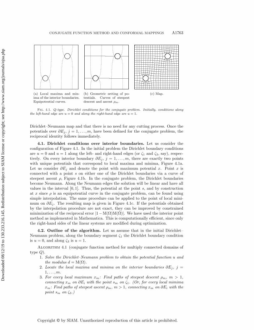
Fig. 4.1. Q-type. Dirichlet conditions for the conjugate problem. Initially, conditions alongthe left-hand edge are u = 0 and along the right-hand edge are u = 1.

Dirichlet--Neumann map and that there is no need for any cutting process. Once thepotentials over \partial Ej , j = 1, . . . ,m, have been defined for the conjugate problem, thereciprocal identity follows immediately.

4.1. Dirichlet conditions over interior boundaries. Let us consider theconfiguration of Figure 4.1. In the initial problem the Dirichlet boundary conditionsare u = 0 and u = 1 along the left- and right-hand edges (or \zeta 1 and \zeta 3, say), respec-tively. On every interior boundary \partial Ej , j = 1, . . . ,m, there are exactly two pointswith unique potentials that correspond to local maxima and minima, Figure 4.1a.Let us consider \partial Ej and denote the point with maximum potential x. Point x isconnected with a point s on either one of the Dirichlet boundaries via a curve ofsteepest ascent \rho , Figure 4.1b. In the conjugate problem, the Dirichlet boundariesbecome Neumann. Along the Neumann edges the solution will be linear and have allvalues in the interval [0, 1]. Thus, the potential at the point s, and by constructionat x since \rho is an equipotential curve in the conjugate problem, can be found usingsimple interpolation. The same procedure can be applied to the point of local mini-mum on \partial Ej . The resulting map is given in Figure 4.1c. If the potentials obtainedby the interpolation procedure are not exact, they can be improved by constrainedminimization of the reciprocal error | 1 - M(\Omega )M(\~\Omega )| . We have used the interior pointmethod as implemented in Mathematica. This is computationally efficient, since onlythe right-hand sides of the linear systems are modified during optimization.

4.2. Outline of the algorithm. Let us assume that in the initial Dirichlet--Neumann problem, along the boundary segment \zeta 1 the Dirichlet boundary conditionis u = 0, and along \zeta 3 is u = 1.

Algorithm 4.1 (conjugate function method for multiply connected domains oftype Q).

1. Solve the Dirichlet--Neumann problem to obtain the potential function u andthe modulus d = M(\Omega ).

2. Locate the local maxima and minima on the interior boundaries \partial Ej, j =1, . . . ,m.

3. For every local maximum xm: Find paths of steepest descent \rho m, m > 1,connecting xm on \partial Ei with the point sm on \zeta 1. (Or, for every local mimimaxm: Find paths of steepest ascent \rho m, m > 1, connecting xm on \partial Ei with thepoint sm on \zeta 3.)

Dow

nloa

ded

08/1

2/19

to 1

30.2

33.2

16.1

45. R

edis

trib

utio

n su

bjec

t to

SIA

M li

cens

e or

cop

yrig

ht; s

ee h

ttp://

ww

w.s

iam

.org

/jour

nals

/ojs

a.ph

p



4. Interpolate the potential on sm on \zeta 1 when \zeta 1 is interpreted as a Neumannedge of the conjugate problem. (Or, similarly on \zeta 3.)

5. Construct the conjugate domain \~\Omega by performing the Dirichlet--Neumann mapon \partial E0 and setting the Dirichlet boundary conditions on \partial Ej, j = 1, . . . ,m,to values obtained in the previous step.

6. Solve the Dirichlet--Neumann problem on \~\Omega for v.7. Construct the conformal mapping \varphi = u+ idv.8. (Optional) Improve the conjugate domain \~\Omega by refining the Dirichlet boundary

conditions via constrained minimization of the reciprocal error | 1 - M(\Omega )M(\~\Omega )| .

5. Numerical implementation of the algorithms. We use the implementa-tion of the hp-FEM method described in detail in [16]. The strategy for computingthe equipotential lines from the canonical domain onto the domain of interest can befound in [15].

The main difference between the two algorithms lies in the cuts between the setsEj , j = 1, 2, . . . ,m, in the case of type R, especially when locating the saddle pointbetween sets. We use the Mathematica built-in constrained optimizer to locate thesaddle points [31]. To find the actual cutting curve, we bisect \partial Ej , j = 1, . . . ,m, andmove against the gradient of u. By doing so, we search for a point on \partial Ej such thatwe end up within a tolerance from the saddle point.

If the cut can be computed analytically, the cut line can be embedded in the apriori mesh, and thus the same mesh can be used in both problems. In this situationit is sufficient to perform elemental integration once. The common blocks in theassembled linear systems can be eliminated as in [15, section 4.2]. In the general case,where the cutting has to be computed numerically, the meshes may vary over largeregions, and the positive bias from reusing the mesh is lost.

For the Q-type, a similar iteration can be used to refine the potential values. Inthis case it may be necessary to refine the geometric search for the potential values.

Our algorithms involve computations that are not usually provided by standardFEM solvers. This is reflected in the relative computation times of the differentparts of the algorithms. The relative maturity and level of implementation vary alot over the solution process. In particular constrained triangulation with possiblylarge curved edges is not available in robust form and in path finding; for instance, indetermining the cuts, the current data structures are not optimal.

6. Numerical experiments. In this section we discuss a series of benchmarkproblems and experiments carefully designed to illustrate different aspects of the al-gorithms. In electrostatics the Q-type refers to resistor design problems with multiplevoltage domains, and the R-type refers to capacitor (electrical condenser) design do-mains. In practice, designing integrated circuits for multiple voltage domains is laborintensive, and there is a need for advanced design systems [20]. We have selectedproblems of both types from the literature and designed the experiments for the R-type. With two exceptions the examples involve multiply connected polycircular-arcdomains. For an alternative solution method for this class of domains, see [6].

The use of the reciprocal relation as an error measure is formalized in the followingdefinition.

Definition 6.1 (reciprocal error). Using Proposition 3.3 we can define twoversions of the reciprocal error. First, for nonnormalized jumps,

(6.1) edr = | 1 - M(\Omega )/M(\~\Omega )| ,

Dow

nloa

ded

08/1

2/19

to 1

30.2

33.2

16.1

45. R

edis

trib

utio

n su

bjec

t to

SIA

M li

cens

e or

cop

yrig

ht; s

ee h

ttp://

ww

w.s

iam

.org

/jour

nals

/ojs

a.ph

p



and second, for the normalized jumps,

(6.2) enr = | 1 - M(\Omega )M(\~\Omega )| .

For convenience we define an associated error order.

Definition 6.2 (error order). Given a reciprocal error e \star r, the positive integer ei,

(6.3) ei = | \lceil log(e \star r)\rceil | ,

is referred to as the error order.

For the general case of R-type, the use of reciprocal error is not straightforward.The cuts must be approximated numerically, and the related approximation error leadsto inevitable consistency error since the jumps depend on the chosen cuts. Thus, inorder to have confidence in the general case as we do for the symmetric cases, oneshould consider a sequence of approximations for the cuts. Here, however, we arecontent to show via the conformal map that the chosen cut is a reasonable one,and the resulting map has the desired characteristics. For the Q-type consistency,error arises from locating the minima and maxima on the interior boundaries andsubsequent determination of the Dirichlet data for the conjugate problems.

Of course, the exact potential functions are not known in general. However, wecan always compute contour plots of the quantities of interest, that is, the absolutevalues of the derivatives, and get a qualitative idea of the overall performance of thealgorithm. Naturally, this also measures the pointwise convergence of the Cauchy--Riemann problem.

One of the advantages of p- and hp-FEM is that exponential convergence incapacity can be achieved even in the case of singularities on the boundary if themesh is graded geometrically. In our implementation the mesh refinement is done viarecursive replacement rules in exact arithmetic, allowing for infinitesimal elements [19].This allows us to generate nearly optimal a priori meshes followed by p refinement.

Data on benchmarks and basic experiments, including representative numbersfor degrees of freedom assuming constant p = 12, is given in Tables 6.1 and 6.2b,respectively. In all cases the setup of the geometry is the most expensive part interms of human effort and time. As usual in p- and hp-FEM, the computational costin these relatively small systems is in integration and handling of the sparse systems.The actual computation times over the set of examples vary from seconds to minuteson standard desktop hardware using our implementation of the algorithms (AppleMac Pro 2009 Edition 2.26 GHz, Mathematica 11.3).

6.1. Benchmarks. In [30] Trefethen gives an excellent introduction to the con-nection between conformal maps and computation of resistances of idealized planarresistors. In our setting the quantity of interest, the resistance of the resistor, isequal to the modulus of the conjugate domain. It should be mentioned that thesebenchmarks could be solved analytically using techniques described in [4].

6.1.1. Computation of resistances for quadrilaterals. Our first benchmarkis of type Q (see Figure 6.1), a resistor first computed in [10]. The domain is enclosedby B = [ - 3/2, 3/2]\times [ - 3/4, 3/4]. There are two square holes (rotated by \pi /4),

H1 = \{ ( - 1/2, 0), ( - 3/4, 1/5), ( - 1, 0), ( - 3/4, - 1/5)\} ,H2 = \{ (1/2, 0), (3/4, - 1/5), (1, 0), (3/4, 1/5)\} ,

Dow

nloa

ded

08/1

2/19

to 1

30.2

33.2

16.1

45. R

edis

trib

utio

n su

bjec

t to

SIA

M li

cens

e or

cop

yrig

ht; s

ee h

ttp://

ww

w.s

iam

.org

/jour

nals

/ojs

a.ph

p



Table 6.1Data on benchmarks.

(a) Computed resistance.

Experiment Capacity Error order (Reference)Resistor 2.841998463680 11 (2.8419984)

(b) Computed capacity. (Error) refers to the reportedestimated error of the reference.

Experiment Capacity (Reference) (Error)Capacitor A 9.49308124 (9.4930811) (4e-7)Capacitor B 8.47016014 (8.4701600) (5e-7)

(c) FEM-data. Mesh (nodes, edges, triangles,quads). Degrees of freedom given at p = 12.

Experiment Mesh DOFResistor (667,1236,16,552) 81935Capacitor A (509,946,8,428) 63143Capacitor B (1013,1910,0,896) 130439

Table 6.2R-type. Data on experiments.

(a) Computed capacities.

Experiment Capacity Error orderThree disks in circle 9.67475429123 12Two disks in rectangle 13.922976299110 12Disk and Pacman in rectangle 13.3376294414 11

(b) FEM-data. Mesh (nodes, edges, triangles, quads). De-grees of freedom given at p = 12.

Experiment Mesh DOFThree disks in circle (35, 52, 0, 18) 2785Two disks in rectangle (34,49,0,16) 2509Disk and Pacman in rectangle (181,320,4,136) 20377

(a) Domain. (b) Mesh. (c) Map.

Fig. 6.1. Resistor.

and indentations

I1 = [ - 3/2, 1/2]\times [ - 3/4, - 1/2], I2 = [ - 1/2, 3/2]\times [1/2, 3/4].

The domain \Omega = B \setminus (H1 \cup H2 \cup I1 \cup I2), with \zeta 1 = along y = 3/4, \zeta 3 = alongy = - 3/4, \zeta 2 = path from ( - 3/2, 3/4) to (1/2, - 3/4), and \zeta 4 = path from (3/2, - 3/4)

Dow

nloa

ded

08/1

2/19

to 1

30.2

33.2

16.1

45. R

edis

trib

utio

n su

bjec

t to

SIA

M li

cens

e or

cop

yrig

ht; s

ee h

ttp://

ww

w.s

iam

.org

/jour

nals

/ojs

a.ph

p



(a) Capacitor A. (b) Capacitor B.

Fig. 6.2. Capacitors.

to ( - 1/2, 3/4). Formally the problems can be stated as(6.4)\left\{

\Delta u = 0 in \Omega ,

u = 0 on \zeta 1,

u = 1 on \zeta 3,

leading to

\left\{ \Delta v = 0 in \~\Omega ,

v = 1 on \zeta 2, v = 0.712841455, on H1,

v = 0 on \zeta 4, v = 0.287158545, on H2.

The computed value of resistance cap(\~\Omega ) = 2.841998463680 is equal to that reportedin [10]. Here we have adopted a convention used throughout in the experiments thatNeumann zero boundary conditions are not defined separately but are implied unlessotherwise specified.

6.1.2. Computation of capacities. We consider two cases, Capacitors A andB, Examples 7 and 10 from [3], respectively (see Figure 6.2). We compute only thecapacities and do not treat these benchmarks as belonging to type R. In both casesthe domain \Omega is enclosed within D = [ - 1, 1]\times [ - 1, 1]. For Capacitor A, the plates aredefined as the union of an equilateral triangle T and its reflection T \prime in the real axis.The vertices of T are the points (a, 0), (b, b - a)/

\surd 3), and (b, - (b - a)/

\surd 3), where

0 < a < b < 1. For Capacitor B, the plates are two slits AsBs and CsDs, definedby points As = ( - 2/3, - 1/2), Bs = ( - 2/3, 1/2), Cs = (1/2, - 1/4), Ds = (1/2, 1/4).The computational domains are \Omega A = D \setminus (T \cup T \prime ) and \Omega B = D \setminus (AsBs \cup CsDs).Thus, the corresponding problems are

(6.5) (A)

\left\{ \Delta u = 0 in \Omega A,

u = 0 on \partial D,

u = 1 on \partial T and \partial T \prime ,

(B)

\left\{ \Delta u = 0 in \Omega B ,

u = 0 on \partial D,

u = 1 on AsBs and CsDs.

Choosing a = 1/5 and b = 7/10, we see that the computed capacity cap(A) =9.49308124 is within the estimated error of the reference value. The computed capacitycap(B) = 8.47016014 is also within the estimated error of the reference value.

6.2. Symmetric case: Three disks in a circle. Consider a unit circle D0

with three disks Di, i = 1, 2, 3, of radius r = 1/6 placed symmetrically so that theirorigins lie on a circle of radius r = 1/2. We set \Omega = D0 \setminus (\cup 3

i=1Di), and \~\Omega containsfive oriented cuts \gamma k enumerated in the order of disks, starting from the outer circle

Dow

nloa

ded

08/1

2/19

to 1

30.2

33.2

16.1

45. R

edis

trib

utio

n su

bjec

t to

SIA

M li

cens

e or

cop

yrig

ht; s

ee h

ttp://

ww

w.s

iam

.org

/jour

nals

/ojs

a.ph

p



(a) Domain. (b) Mesh. (c) Map.

(d) Cauchy--Riemann. Contourlines of | \partial u/\partial x| and | \partial v/\partial y| .

2 3 4 5 6 7 8 9 10 11 12 13 14

10-1210-1110-1010-910-810-710-610-510-410-310-210-1

(e) Reciprocal identity. Conver-gence in p; log-plot, error versusp.

Fig. 6.3. R-type. Fully symmetric case.

D0, D0D1D2D3D1D0. Using symmetry for the jumps, the problems can be writtenas(6.6)\left\{


u = 0 on \partial D0,

u = 1 on \cup 3i=1 \partial Di,

leading to


v = 0 on \gamma 1,

v = R/6 + (k - 2)R/3 on \gamma k, k = 2, 3, 4,

v = R = 9.67475429123 on \gamma 5.

As indicated in Figure 6.3a the cut can be computed analytically. The blendingfunction approach used to compute higher order curved elements is very accurate ifthe element edges meet the curved edges at right angles. This is the reason for themesh in Figure 6.3b where all edges adjacent to disks have been set optimally.

Notice that due to symmetry, the scaled jumps could also be computed analyt-ically. However, in the numerical experiments, only computed values of Table 6.2aare used. Since the cuts are embedded in the mesh lines, both problems (the originaland the conjugate) can be solved using the same mesh. In this optimal configuration,convergence in reciprocal relation is exponential in p, which is a remarkable result;see Figure 6.3e. Similarly, in Figure 6.3d, it is clear that the derivatives also haveconverged over the whole domain.

6.3. Axisymmetric cases. In the next three cases we maintain axial symmetryand thus analytic cuts. In the first two cases the enclosing rectangle R = [ - 1, 3] \times [ - 1, 1], and in the third case RP = [ - 2, 1]\times [ - 1, 1].

Dow

nloa

ded

08/1

2/19

to 1

30.2

33.2

16.1

45. R

edis

trib

utio

n su

bjec

t to

SIA

M li

cens

e or

cop

yrig

ht; s

ee h

ttp://

ww

w.s

iam

.org

/jour

nals

/ojs

a.ph

p



-1 0 1 2 3

-1.0

-0.5

0.0

0.5

1.0

(a) Cauchy--Riemann. Contourlines of | \partial u/\partial x| and | \partial v/\partial y| .

-1 0 1 2 3-1.0

-0.5

0.0

0.5

1.0

(b) Cauchy--Riemann. Contourlines of | \partial u/\partial x| and | \partial v/\partial y| .

2 3 4 5 6 7 8 9 10 11 12 13

10-1310-1210-1110-1010-910-810-710-610-510-410-310-2

(c) Two disks in rectangle. Re-ciprocal identity. Convergence inp; log-plot, error versus p.

2 3 4 5 6 7 8 9 10 11 12 13

10-11

10-10

10-9

10-8

10-7

10-6

10-5

10-4

10-3

(d) Disk and Pacman in rectan-gle. Reciprocal identity. Conver-gence in p; log-plot, error versusp.

Fig. 6.4. R-type. Axially symmetric cases.

6.3.1. Two disks in a rectangle. Consider two disks D1 and D2 of radius= 1/2 with centers at (0, 0) and (2, 0), respectively. Here \Omega = R \setminus (\cup 2

i=1Di) and \~\Omega contains four oriented cuts \gamma k enumerated in the order of regions starting from R,RD1D2D1R, and the problems can be stated as(6.7)\left\{


u = 0 on \partial R,

u = 1 on \cup 2i=1 \partial Di,

leading to


v = 0 on \gamma 1,

v =M/4 + (k - 2)M/2 on \gamma k, k = 2, 3,

v =M = 13.922976299110 on \gamma 4.

The scaled jumps can be computed analytically, of course. The location of the saddlepoint is xs = (1, 0) and the corresponding value of u(xs) = 0.747496. Once again, thereciprocal convergence in p is exponential (see Figure 6.4c). Similarly, the derivativesshow convergence (see Figure 6.4a).

6.3.2. Disk and Pacman in rectangle. Next, the disk D2 above is replacedby a disk with one quarter cut, C1, the so-called Pacman. Now \Omega = R \setminus (D1 \cup C1),and \~\Omega contains four oriented cuts \gamma k enumerated in the order of regions starting fromR, RD1C1D1R,

(6.8)

\left\{ \Delta u = 0 in \Omega ,

u = 0 on \partial R,

u = 1 on \partial D1 \cup \partial C1,

leading to


v = 0 on \gamma 1,

v =\sum k - 1

j=1 dj on \gamma k, k = 2, 3, 4.

In this case we intentionally break the symmetry between meshes for the two

Dow

nloa

ded

08/1

2/19

to 1

30.2

33.2

16.1

45. R

edis

trib

utio

n su

bjec

t to

SIA

M li

cens

e or

cop

yrig

ht; s

ee h

ttp://

ww

w.s

iam

.org

/jour

nals

/ojs

a.ph

p



problems. The geometric refinement at the re-entrant corners is done in slightlydifferent ways. The reciprocal convergence in p is exponential but with different ratesat lower and higher values of p. Also, the difference in the number of refinement levelsleads to a mild consistency error which appears as a loss of further convergence andaccuracy at high p (see Figure 6.4d).

Here the jumps must be computed numerically (and tested against the computedcapacity). Jumps have four decimals,

d1 = 3.4808, d2 = 6.3761, d3 = 3.4808,

with cap(\Omega ) = 13.3376294414. The location of the saddle point is xs = (1, 0), and thecorresponding value of u(xs) = 0.747475, which does differ from the value observedfor two circles. Again, the derivatives show convergence despite the re-entrant corners(see Figure 6.4b).

6.3.3. Pacman and droplet: Domain with cusp. Now the interior regionsare a Pacman C at (0, 0), and a domain B bounded by a Bezier curve,

r(t) =1

640

\bigl( 45t6 + 75t4 - 525t2 + 469

\bigr) +

15

32t\bigl( t2 - 1

\bigr) 2, t \in [ - 1, 1].

Let us first consider a corresponding problem of R-type. Let \Omega = RP \setminus (C \cup B),and \~\Omega contains four oriented cuts \gamma i enumerated in the order of regions starting fromRP , RPCBCRP ,

(6.9)


u = 0 on \partial D0,

u = 1 on \partial D1,2,3,

leading to


v = 0 on \gamma 1,

v =\sum k - 1

j=1 dj on \gamma k, k = 2, 3, 4.

In [15] a ring domain with the same curve was considered up to very high accuracy.Notice that the ``droplet"" is designed so that also the tangents are aligned for param-eter values t = \pm 1, and thus the opening angle is 2\pi requiring strong grading of themesh. The resulting map is shown in Figure 6.5d. Letting p = 16 and using 14 levelsof refinement at the three singularities, we see that the computed jumps are

d1 = 3.3449, d2 = 4.08337, d3 = 3.3449,

with cap(\Omega ) = 10.7732. The location of the saddle point is xs = ( - 0.199, 0), and thecorresponding value of u(xs) = 0.7540. The error order = 6.

Next we set up a corresponding problem of Q-type as follows: \zeta 1 = along x = - 1,\zeta 2 = along y = - 1, \zeta 3 = along x = 3, \zeta 4 = along y = 1,

(6.10)


u = 0 on \zeta 1,

u = 1 on \zeta 3,

leading to


v = 0 on \zeta 2, v = 1/2, on C,

v = 1 on \zeta 4, v = 1/2, on B.

Again letting p = 16 and using 14 levels of refinement at the three singularities, weget cap(\Omega ) = 0.496668 and cap(\~\Omega ) = 2.01353, resulting in error order = 7. The mapis shown in Figure 6.5e. The corresponding horizontal or u-coordinates of the slitsare

\{ (0.0643908, 0.640592), (0.75947, 0.962074)\} .Interestingly, in the R-type problem the error order decreases only slightly in

comparison despite the numerical estimation of the jumps.

Dow

nloa

ded

08/1

2/19

to 1

30.2

33.2

16.1

45. R

edis

trib

utio

n su

bjec

t to

SIA

M li

cens

e or

cop

yrig

ht; s

ee h

ttp://

ww

w.s

iam

.org

/jour

nals

/ojs

a.ph

p



(a) R-type. Disk and Pacman. (b) Mesh. (c) Map.

(d) R-type. Pacman and droplet. (e) Q-type. Pacman and droplet.

Fig. 6.5. Axially symmetric cases.

7. Advanced examples. Our last two examples illustrate the versatility of ourapproach in problems where the cuts have to be computed numerically or the domainsare not polycircular-arc.

7.1. \bfitR -type with multiple regions. Let us consider a case with seven regions,five circles Ci, and two triangles Tj (Figure 7.1) scattered in the unit square. Thereare six saddle points sk. The exact locations are given in Table 7.1. In this case alsothe cuts have to be computed numerically, and thus finding the saddle points is thecrucial first step. Once the cuts have been identified, they must be embedded intothe conjugate mesh. In contrast with the previous cases, the mesh lines cannot beenforced a priori. In this case we have chosen to approximate the cuts with linearsegments rather than curves, which would be more natural in the p-version setting.This is due to maturity of the tools available for constrained triangulation.

Since the geometric complexity is greater, the algorithm naturally does moregeometric computations and consequently operates outside the fast kernels, such aslinear algebra routines. In this particular case, locating the saddle points took oneminute and finding cuts an additional four minutes, in contrast to two minutes spentin integration, which is the typical bottleneck in p-version computations.

The derived results are summarized in Figures 7.1 and 7.2. We get cap(\Omega ) =14.2324 with error order = 2. The error order is slightly disappointing, especiallyin comparison with our other experiments. In addition to errors from geometricapproximation, there is also an additional source of error, namely the integrationof the jumps when one contour line intersects multiple jumps, since one has to relyon pointwise evaluation of both the potentials and their derivatives. Convergencein capacity does not imply the same pointwise convergence rates. For instance, forthe largest region there are four cuts emanating from it. Thus, the resolution of thecontour lines is also something one should consider.

Dow

nloa

ded

08/1

2/19

to 1

30.2

33.2

16.1

45. R

edis

trib

utio

n su

bjec

t to

SIA

M li

cens

e or

cop

yrig

ht; s

ee h

ttp://

ww

w.s

iam

.org

/jour

nals

/ojs

a.ph

p



0.0 0.2 0.4 0.6 0.8 1.00.0

0.2

0.4

0.6

0.8

1.0

(a) The initial mesh.

0.0 0.2 0.4 0.6 0.8 1.00.0

0.2

0.4

0.6

0.8

1.0

(b) Contour plot of u with cutsand saddle points indicated.

0.0 0.2 0.4 0.6 0.8 1.00.0

0.2

0.4

0.6

0.8

1.0

(c) The conjugate mesh.

0.0 0.2 0.4 0.6 0.8 1.00.0

0.2

0.4

0.6

0.8

1.0

(d) Map.

Fig. 7.1. R-type. Multiple regions. The boundary of the conjugate mesh can be traced bystarting from the bottom and keeping the interior to the left.

Table 7.1R-type. Multiple regions. There are five circles ci defined by their centers and radii, two

triangles Tj by their corner points (A,B,C), and six saddle points sk by their locations (x, y).

C (x, y) rc1 (0.3, 0.5) 1/10c2 (0.6, 0.25) 1/15c3 (0.75, 0.6) 1/15c4 (0.3, 0.75) 1/20c5 (0.2, 0.2) 1/20

T1 T2

A (3/4, 3/4) (17/20, 3/20)B (17/20, 3/4) (9/10, 3/20)C (4/5, 4/5) (9/10, 1/5)

S (x, y)s1 (0.51, 0.40)s2 (0.27, 0.29)s3 (0.32, 0.66)s4 (0.60, 0.51)s5 (0.79, 0.22)s6 (0.77, 0.71)

7.2. \bfitQ -type with nonsymmetric configuration. Let us consider a Q-typeproblem where the domain B0 is enclosed by a parametrized curve,

r(t) =1

5(4 + cos(5t))(cos(t)i+ sin(t)j),

with three scaled copies Bi = 110r(t) + bi scattered within it, where the offsets are

b1 = - (1/10, 1/5), b2 = (1/20, 2/5), b3 = (2/5, 1/15). The computational domain\Omega = B0 \setminus (\cup 3

i=1Bi). The boundary curve r(t) is divided into four oriented arcs \zeta i with

Dow

nloa

ded

08/1

2/19

to 1

30.2

33.2

16.1

45. R

edis

trib

utio

n su

bjec

t to

SIA

M li

cens

e or

cop

yrig

ht; s

ee h

ttp://

ww

w.s

iam

.org

/jour

nals

/ojs

a.ph

p



1 2 3 4 5 6 7 8 9 10 11 12 13 14u \ast 0.90 0.97 0.97 0.93 0.96 0.96 0.93 0.95 0.74 0.74 0.95 0.90 \ast v 0 0.17 0.23 0.36 0.38 0.40 0.53 0.62 0.62 0.64 0.82 0.93 0.94 1

(a) Data over the cuts. u is the potential at the saddle point; v is the Dirichlet boundary data.

1

d

0

(b) Canonical domain in (u, v).Slit domain scaled to d = 1.

Fig. 7.2. R-type. Multiple regions. Canonical domain and configuration data.

points

qi = \{ (0.997045, 0.0313334), ( - 0.0241459, 0.768334),

( - 0.602165, - 0.0189238), (0.0261114, - 0.830877)\} .

So, the problem can be stated as

(7.1)


u = 0 on \zeta 1,

u = 1 on \zeta 3,

leading to


v = 0 on \zeta 2, v = v1, on B1,

v = 1 on \zeta 4, v = v2, on B2,

v = v3 on B3.

The initial mesh is piecewise linear and thus not exact in the sense of the examplesabove. In Figure 7.3d we let p = 2, . . . , 16 and show the convergence graph of thereciprocal error (loglog). The observed rate is 1.87, indicating algebraic convergence.The initial computed Dirichlet boundary conditions for the conjugate problem are

v1 = 0.403375, v2 = 0.592293, v3 = 0.323098,

and after five steps of the interior point method, are corrected to

v1 = 0.501596, v2 = 0.736346, v3 = 0.358485,

and the corresponding horizontal or u-coordinates of the slits are

\{ (0.588018, 0.831274), (0.1605, 0.43309), (0.128553, 0.416906)\} .

We get cap(\Omega ) = 0.908799, cap(\~\Omega ) = 1.101067, and error order = 4. The meshhas 2689 nodes, 7273 edges, and 4582 triangles. In this case, when p = 4 the time

Dow

nloa

ded

08/1

2/19

to 1

30.2

33.2

16.1

45. R

edis

trib

utio

n su

bjec

t to

SIA

M li

cens

e or

cop

yrig

ht; s

ee h

ttp://

ww

w.s

iam

.org

/jour

nals

/ojs

a.ph

p



-0.5 0.0 0.5 1.0

-0.5

0.0

0.5

1.0

(a) Domain with the four cornersof the quadrilateral and the localmaxima and minima indicated.

-0.5 0.0 0.5 1.0

-0.5

0.0

0.5

1.0

(b) Mesh.

-0.5 0.0 0.5 1.0

-0.5

0.0

0.5

1.0

(c) Map.

●

●

●

●●

●●

●●

●●●●●●

100 101

10-3

10-2

100 101

10-3

10-2

p

Reciprocalerror

(d) Convergence of the reciprocal error in p \in [2, 16]; loglog-plot, rate = 1.87.

Fig. 7.3. Q-type. Domain enclosed by a parametrized curve r(t) = 15(4 + cos(5t))(cos(t)i +

sin(t)j).

to determine the Dirichlet boundary conditions for the conjugate problem was onlyfour seconds, whereas the integration took 11 seconds, with the initial linear solutiontaking an additional two seconds, and five steps of the interior point method took 20seconds.

8. Conclusions. We have introduced algorithms for computation of conformalmappings in multiply connected domains for two specific classes of problems. However,the fundamental ideas can be applied to address a much wider class of problems.Our method relies on numerical solution of PDEs and therefore can be applied togeneral domains using standard tools with the addition of geometric operations, suchas finding paths of steepest descent. In terms of computational cost, the method iscompetitive, especially in cases where the p-version of FEM can be applied directly.In our current implementation the geometric operations become expensive as thecomplexity of the configuration increases.

Acknowledgments. The authors wish to thank Professor R. Michael Porter forhis careful reading of an earlier version of this manuscript. The authors also wishto thank Professor T. DeLillo and Dr. E. Kropf for help in setting up the exampleof section 6.1.1. Finally, we wish to thank the anonymous referees, who helped usimprove this paper considerably.

Dow

nloa

ded

08/1

2/19

to 1

30.2

33.2

16.1

45. R

edis

trib

utio

n su

bjec

t to

SIA

M li

cens

e or

cop

yrig

ht; s

ee h

ttp://

ww

w.s

iam

.org

/jour

nals

/ojs

a.ph

p



REFERENCES

[1] L.V. Ahlfors, Conformal invariants: Topics in geometric function theory, McGraw-Hill BookCo., 1973.

[2] L.V. Ahlfors, Complex Analysis. An Introduction to the Theory of Analytic Functions of OneComplex Variable, 3rd ed., Internat. Ser. Pure Appl. Math., McGraw-Hill Book Co., 1978.

[3] D. Betsakos, K. Samuelsson, and M. Vuorinen, The computation of capacity of planarcondensers, Publ. Inst. Math. (Beograd) (N.S.), 75(89) (2004), pp. 233--252.

[4] D.G. Crowdy, The Schwarz-Christoffel mapping to bounded multiply connected polygonal do-mains, Proc. R. Soc. Lond. Ser. A Math. Phys. Eng. Sci., 461 (2005), pp. 2653--2678.

[5] D.G. Crowdy, Schwarz-Christoffel mappings to unbounded multiply connected polygonal re-gions, Math. Proc. Cambridge Philos. Soc., 142 (2007), pp. 319--339.

[6] D.G. Crowdy, A.S. Fokas, and C.C. Green, Conformal mappings to multiply connectedpolycircular arc domains, Comput. Methods Funct. Theory, 11 (2012), pp. 685--706.

[7] D.G. Crowdy and C.C. Green, The Schottky-Klein Prime Function MATLAB Files, http://www2.imperial.ac.uk/\sim dgcrowdy/SKPrime, 2010.

[8] D.G. Crowdy and J.S. Marshall, Computing the Schottky-Klein prime function on theSchottky double of planar domains, Comput. Methods Funct. Theory, 7 (2007), pp. 293--308.

[9] T.K. DeLillo, A.R. Elcrat, and J.A. Pfaltzgraff, Schwarz-Christoffel mapping of multiplyconnected domains, J. Anal. Math., 94 (2004), pp. 17--47.

[10] T.K. DeLillo, A.R. Elcrat, and E.H. Kropf, Calculation of resistances for multiply con-nected domains using Schwarz-Christoffel transformations, Comput. Methods Funct. The-ory, 11 (2012), pp. 725--745.

[11] T.A. Driscoll, A MATLAB toolbox for Schwarz-Christoffel mapping, ACM Trans. Math.Software, 22 (1996), pp. 168--186.

[12] T.A. Driscoll, The Schwarz-Christoffel Toolbox for MATLAB, http://www.math.udel.edu/\sim driscoll/SC/, 2009.

[13] T.A. Driscoll and L.N. Trefethen, Schwarz-Christoffel Mapping, Cambridge Monogr. Appl.Comput. Math. 8, Cambridge University Press, 2002.

[14] H. Grunsky, Lectures on Theory of Functions in Multiply Connected Domains, Vandenhoeck\& Ruprecht, 1978.

[15] H. Hakula, T. Quach, and A. Rasila, Conjugate function method for numerical conformalmappings, J. Comput. Appl. Math., 237 (2013), pp. 340--353.

[16] H. Hakula, A. Rasila, and M. Vuorinen, On moduli of rings and quadrilaterals: Algorithmsand experiments, SIAM J. Sci. Comput., 33 (2011), pp. 279--302, https://doi.org/10.1137/090763603.

[17] H. Hakula, A. Rasila, and M. Vuorinen, Computation of exterior moduli of quadrilaterals,Electron. Trans. Numer. Anal., 40 (2013), pp. 436--451.

[18] H. Hakula, A. Rasila, and M. Vuorinen, Conformal modulus and planar domains withstrong singularities and cusps, Electron. Trans. Numer. Anal., 48 (2018), pp. 462--478.

[19] H. Hakula and T. Tuominen, Mathematica implementation of the high order finite elementmethod applied to eigenproblems, Computing, 95 (2013), pp. 277--301.

[20] J.A. Iadanza, R. Singh, S.T. Ventrone, and I.L. Wemple, Method for Designing an Inte-grated Circuit Having Multiple Voltage Domains, US Patent 7,000,214, filed November 19,2003, and issued February 14, 2006.

[21] P. Koebe, Abhandlungen zur Theorie der konformen Abbildung. IV. Abbildung mehrfachzusammenh\"angender schlichter Bereiche auf Schlitzbereiche, Acta Math., 41 (1916),pp. 305--344.

[22] O. Lehto and K.I. Virtanen, Quasiconformal Mappings in the Plane, Springer, Berlin, 1973.[23] W. Luo, J. Dai, X. Gu, and S.-T. Yau, Numerical conformal mapping of multiply connected

domains to regions with circular boundaries, J. Comput. Appl. Math., 233 (2010), pp. 2940--2947.

[24] A. Mayo, Rapid methods for the conformal mapping of multiply connected regions, J. Comput.Appl. Math., 14 (1986), pp. 143--153.

[25] Z. Nehari, Conformal Mapping, McGraw-Hill Book Co., 1952.[26] N. Papamichael and N.S. Stylianopoulos, Numerical Conformal Mapping: Domain De-

composition and the Mapping of Quadrilaterals, World Scientific, 2010.[27] L. Reichel, A fast method for solving certain integral equations of the first kind with applica-

tion to conformal mapping, J. Comput. Appl. Math., 14 (1986), pp. 125--142.[28] O. S\'ete and J. Liesen, On conformal maps from multiply connected domains onto lemniscatic

domains, Electron. Trans. Numer. Anal., 45 (2016), pp. 1--15.

Dow

nloa

ded

08/1

2/19

to 1

30.2

33.2

16.1

45. R

edis

trib

utio

n su

bjec

t to

SIA

M li

cens

e or

cop

yrig

ht; s

ee h

ttp://

ww

w.s

iam

.org

/jour

nals

/ojs

a.ph

p

http://www2.imperial.ac.uk/~dgcrowdy/SKPrime

http://www2.imperial.ac.uk/~dgcrowdy/SKPrime

http://www.math.udel.edu/~driscoll/SC/

http://www.math.udel.edu/~driscoll/SC/

https://doi.org/10.1137/090763603

https://doi.org/10.1137/090763603



[29] L.N. Trefethen, Numerical computation of the Schwarz--Christoffel transformation, SIAM J.Sci. Stat. Comput., 1 (1980), pp. 82--102, https://doi.org/10.1137/0901004.

[30] L.N. Trefethen, Analysis and design of polygonal resistors by conformal mapping, Z. Angew.Math. Phys., 35 (1984), pp. 692--704.

[31] Wolfram Research, Inc., Mathematica, Version 11.3, 2018.[32] W. Zeng, X. Yin, M. Zhang, F. Luo, and X. Gu, Generalized Koebe's method for confor-

mal mapping multiply connected domains, in Proceedings of the 2009 SIAM/ACM JointConference on Geometric and Physical Modeling, ACM, 2009, pp. 89--100.

Dow

nloa

ded

08/1

2/19

to 1

30.2

33.2

16.1

45. R

edis

trib

utio

n su

bjec

t to

SIA

M li

cens

e or

cop

yrig

ht; s

ee h

ttp://

ww

w.s

iam

.org

/jour

nals

/ojs

a.ph

p

https://doi.org/10.1137/0901004

Hakula, Harri; Quach, Tri; Rasila, Antti The Conjugate ...

Documents

Transcript of Hakula, Harri; Quach, Tri; Rasila, Antti The Conjugate ...