Groundwater Vulnerability and Risk Mapping Based on ...
29
HAL Id: insu-01237105 https://hal-insu.archives-ouvertes.fr/insu-01237105 Submitted on 20 Jan 2016 HAL is a multi-disciplinary open access archive for the deposit and dissemination of sci- entific research documents, whether they are pub- lished or not. The documents may come from teaching and research institutions in France or abroad, or from public or private research centers. L’archive ouverte pluridisciplinaire HAL, est destinée au dépôt et à la diffusion de documents scientifiques de niveau recherche, publiés ou non, émanant des établissements d’enseignement et de recherche français ou étrangers, des laboratoires publics ou privés. Distributed under a Creative Commons Attribution - NonCommercial - NoDerivatives| 4.0 International License Groundwater Vulnerability and Risk Mapping Based on Residence Time Distributions: Spatial Analysis for the Estimation of Lumped Parameters Myriam Dedewanou, Stéphane Binet, Jean-Louis Rouet, Yves Coquet, Ary Bruand, Hervé Noel To cite this version: Myriam Dedewanou, Stéphane Binet, Jean-Louis Rouet, Yves Coquet, Ary Bruand, et al.. Ground- water Vulnerability and Risk Mapping Based on Residence Time Distributions: Spatial Analysis for the Estimation of Lumped Parameters. Water Resources Management, Springer Verlag, 2015, 29 (15), pp.5489-5504. 10.1007/s11269-015-1130-8. insu-01237105
Transcript of Groundwater Vulnerability and Risk Mapping Based on ...
HAL Id: insu-01237105https://hal-insu.archives-ouvertes.fr/insu-01237105
Submitted on 20 Jan 2016
HAL is a multi-disciplinary open accessarchive for the deposit and dissemination of sci-entific research documents, whether they are pub-lished or not. The documents may come fromteaching and research institutions in France orabroad, or from public or private research centers.
L’archive ouverte pluridisciplinaire HAL, estdestinée au dépôt et à la diffusion de documentsscientifiques de niveau recherche, publiés ou non,émanant des établissements d’enseignement et derecherche français ou étrangers, des laboratoirespublics ou privés.
Distributed under a Creative Commons Attribution - NonCommercial - NoDerivatives| 4.0International License
Groundwater Vulnerability and Risk Mapping Based onResidence Time Distributions: Spatial Analysis for the
Estimation of Lumped ParametersMyriam Dedewanou, Stéphane Binet, Jean-Louis Rouet, Yves Coquet, Ary
Bruand, Hervé Noel
To cite this version:Myriam Dedewanou, Stéphane Binet, Jean-Louis Rouet, Yves Coquet, Ary Bruand, et al.. Ground-water Vulnerability and Risk Mapping Based on Residence Time Distributions: Spatial Analysis forthe Estimation of Lumped Parameters. Water Resources Management, Springer Verlag, 2015, 29 (15),pp.5489-5504. �10.1007/s11269-015-1130-8�. �insu-01237105�
1
Groundwater vulnerability and risk 1
mapping based on Residence Time 2
Distributions: Spatial analysis for the 3
estimation of lumped parameters 4
5
6 M. Dedewanou 1,2, S. Binet 1, 3, JL. Rouet1, Y. Coquet1, A. Bruand1, H. Noel2 7
1 ISTO, UMR 7327 CNRS-Université d’Orléans-BRGM, 45071 Orléans cedex 2 8
2 GEO-HYD, 101 rue Jacques Charles, 45160, Olivet, France. 9
3 ECOLAB, UMR 5245 CNRS-UPS-INPT, 31326 Castanet-Tolosan, France 10
__________________________________________________________________________ 11
Abstract 12
Specific vulnerability estimations for groundwater resources are usually geographic 13
information system-based (GIS) methods that establish spatial qualitative indexes which 14
determine the sensitivity to infiltration of surface contaminants, but with little validation of the 15
working hypothesis. On the other hand, lumped parameter models, such as the Residence 16
Time Distribution (RTD), are used to predict temporal water quality changes in drinking water 17
supply, but the lumped parameters do not incorporate the spatial variability of the land cover 18
and use. At the interface between these two approaches, a GIS tool was developed to estimate 19
the lumped parameters from the vulnerability mapping dataset. In this method the temporal 20
evolution of groundwater quality is linked to the vulnerability concept on the basis of equivalent 21
lumped parameters that account for the spatially distributed hydrodynamic characteristics of 22
the overall unsaturated and saturated flow nets feeding the drinking water supply. This 23
vulnerability mapping method can be validated by field observations of water concentrations. 24
A test for atrazine specific vulnerability of the Val d’Orléans karstic aquifer demonstrates the 25
reliability of this approach for groundwater contamination assessment. 26
2
Keywords: Specific vulnerability, advection / dispersion, residence time distribution, equivalent 27
parameters. 28
1. Introduction 29
The main tools for the management and the conservation of groundwater resources consist in 30
characterizing the vulnerability of the aquifer used for drinking water. Intrinsic vulnerability uses 31
physical characteristics as criteria to determine the sensitivity of groundwater to surface 32
pollution. Most intrinsic vulnerability maps are multi-criteria, weighted and index-based, 33
developed by Aller et al., (1987), Doerfliger et al., (1999), Petelet-Giraud et al., (2001) and 34
Civita and De Maio (2004). The specific vulnerability of groundwater incorporates the physico-35
chemical properties and their relationship with the natural environment as supplementary 36
criteria in the vulnerability index estimation (Vrba and Zaporozec, 1994). These tools enable 37
policies for the development of codes of practice for groundwater protection to be proposed 38
(Escolero et al. 2002) and open up significant opportunities to enhance the efficacy of water 39
vulnerability assessment tools by incorporating indicators and operational measures for social 40
considerations (Plummer et al., 2012). While the area of use is huge, the index calculation 41
method is limited because the weighting is usually arbitrarily chosen. These approaches are 42
qualitative and highly subject to the hydrogeologist's interpretation (Panagopoulos et al., 43
2006). 44
Borehole vulnerability analysis was developed for drinking water supplying watersheds. This 45
method completes the vulnerability index with the notions of distance, horizontal flow rate and 46
transport to the target (borehole or spring) (Goldscheider and Popescu, 2003). In this 47
framework, two types of vulnerability can be defined: a resource vulnerability which only takes 48
vertical transfer into account, and a borehole vulnerability which incorporates the horizontal 49
transfer into the borehole. The key parameters for the evaluation of specific vulnerability are 50
the residence time of contaminants, their capacity of migration underground and the 51
3
attenuation process. Some authors (Neukum et al., 2008; Anderson and Gosk 1987; Sadek 52
and Abd El-Samie, 2001; Bakalowicz, 2005) suggested that a high vulnerability is related to a 53
short residence time of the main part of the recharge. From these concepts, Brouyère (2001) 54
relate a potential contamination to the transfer time, concentration level and duration of the 55
phenomenon, plotted along the three axe of the cube. Jeannin et al. (2001) developed a 56
program that relates field observations to concentration level, transfer time and duration. The 57
model assumes an instantaneous release of a conservative contaminant at a given point on 58
the land surface and simulates the resulting breakthrough curves at the outlet of each sub-59
system by means of the advection - dispersion equation, disregarding retardation and 60
degradation processes (Zwahlen, 2003). 61
By linking the vulnerability index to physical parameters, the working hypothesis used in 62
vulnerability mapping can be tested. Goldscheider et al. (2001) released different tracers at 63
the land surface and observed the breakthrough at a target (spring), the travel time, the 64
concentration and the tracer recovery rate to validate a vulnerability map. Holman et al. (2005) 65
validated an intrinsic groundwater vulnerability method using a national nitrate database and 66
some co-variance and variance analyses. Neukum et al. (2008) worked on the validation of a 67
vulnerability map based on field investigation and column tracer experiments conducted on 68
soil materials. The authors modelled tracer displacements using the advection – dispersion 69
model and proposed a transit time distribution function of the tracer that depends on the 70
geometric and hydraulic boundary conditions of the aquifer. Lasserre et al. (1999) developed 71
a simple GIS-linked model to describe the groundwater transport of nitrates. For all these 72
methods, developed to validate vulnerability criteria, the aim was to link surface land use with 73
watershed hydrodynamic properties and water quality at the boreholes. 74
For time series analysis, several studies have applied an impulse response at the watershed 75
scale for solute transport modeling purposes (Jury, 1982; Beltman et al., 1994; Barry and 76
Parker, 1987; Molénat et al., 1999; Schwientek et al., 2009). The method consists in 77
establishing a residence time distribution (RTD) to link pollutants at the surface of the 78
4
watershed to the contaminant concentrations measured in the borehole. Related to the 79
geometry of the aquifer, Jurgens et al., (2012) proposed six theoretical models, (derived from 80
analytical solutions of the advection - dispersion reaction equation) to fit the impulse response 81
with three lumped parameters. These parameters vary from one study to another, but the ones 82
most widely used are the average residence time, the Peclet number and the rate of 83
degradation. To evaluate groundwater quality trends, Visser et al. (2009) after a comparison 84
between statistical, groundwater dating and deterministic modeling, showed that impulse 85
response methods require little information about the physical system, but rather rely on the 86
available data, which makes them suitable for application to a wide variety of systems. 87
Linking the spatial properties that determine the vulnerability and the temporal evolution of the 88
water quality is a key point for water resource management. At the watershed scale, some 89
semi-distributed models incorporate the soil surface properties to model water quality with a 90
GIS dataset based on an impulse response, such as the SWAT model (Srinivasan and Arnold, 91
1994) or on a flow model such as Drainmod (Fernandez et al. 2006) MACRO (Larsbo and 92
Jarvis, 2003) and STICS (Ledoux, 2003). For groundwater quality purposes, the flow paths 93
must be analyzed in 3 dimensions but few tools are available to compute an impulse response 94
from the spatially distributed 3D groundwater properties. 95
This paper proposes a method to calculate a RTD impulse response in aquifers based on 96
spatial datasets used for specific vulnerability assessments. The spatial GIS vulnerability 97
dataset corresponds to the thickness and hydrodynamic parameters of the geological 98
formations found along the groundwater flow nets. 99
Based on the impulse response, which is characteristic of the watershed, the vulnerability 100
index is defined as the mass ratio between the contaminants that exceeds a fixed threshold at 101
the borehole and the injected mass. This makes it possible to map the relative vulnerability of 102
each infiltration surface where contaminant application occurs. This approach includes 103
residence times, dispersion and attenuation. Spatial vulnerability mapping is validated with GIS 104
using the temporal evolution of the groundwater quality. 105
5
106
2. The Residence Time Distribution (RTD) 107
The Residence Time Distribution (RTD) is a probability distribution function that describes the 108
amount of time a fluid element can spend inside the column. After a pulse of mass 𝑀, its RTD 109
is defined as : 110
E(t) =Q C(t)
M =
M (t)
M (Equation 1) 111
Here 𝑄 [L3.T-1] is the discharge flowing through the column. 112
The concentration C(t) [M.L-3] can be obtained by solving the transport equation along a 113
column open at both ends (Kreft and Zuber, 1978). For the transport of a pulse of mass 𝑀 in 114
a porous one-dimensional column (the transversal section is 𝐴 [L²], the length 𝑥 and the column 115
water content is 𝜃), where water flow with a velocy (u) there is many analytical solutions, most 116
of them use the non-dimensional Peclet number (Pe), the average residence time (t ̅) and the 117
rate of degradation λ [T-1] of the contaminant during transport. 118
To assume that the column is open at both ends (Levenspiel 1962, Maloszewski and Zuber, 119
1982) enables to express the RTD as follow: 120
E(t) = √Pe
4πtt̅exp [-
Pe (t̅-t)²
4tt̅] exp [- t ] (Equation 2) 121
The contaminant transport through the column is described with only three parameters and no 122
assumption is made on the laminar, turbulent, unsaturated or saturated nature of the flows. 123
Degradation and delay are taken into account with and 𝑡̅. If no reaction occurs, 𝑡̅ is the same 124
as the average residence time of the water in the column. 125
2.1. RTD for a column with multi layers. 126 127
6
For the transport of a pulse, the mean residence time t̅ [T] of the contaminant in the column 128
can be defined either with the 𝐶(𝑡) curve or as the ratio between the water flux (u) and the 129
stored water (θ L): 130
t ̅ =∫ t C(t) dt
∞0
∫ C(t)dt∞
0
=u
θ L (Equation 3) 131
Another important descriptor of the 𝐶(𝑡) curve is its variance: 132
𝜎2 = ∫ (t−t̅)² C(t) dt
∞0
∫ C(t)dt∞
0
(Equation 4) 133
In decomposing the borehole watershed into n parallel flow nets. This reduces the non-linear 134
three-dimensional problem to a linear one-dimensional one. The water and the contaminant 135
mass which infiltrate the ground enter through the various 𝑖 layers of the aquifer where the 136
hydro-dispersive properties can vary. They flow through the 𝑖 layers until the borehole, 137
following the flow nets. For every 𝑛 flow net, the 𝑖 layers are considered to be independent 138
columns characterized by the average residence time 𝑡�̅�,𝑖 and the Peclet number 𝑃𝑒𝑛,𝑖. 139
For 𝑖 serial layers, equivalent properties can be calculated. The mean residence time for the 140
𝑛th flow net, where contaminant flows through 𝑖 serial columns, is: 141
⟨t̅n⟩ = ∑ t̅n,ii1 (Equation 5) 142
In 1959, Aris showed that, in the case of an infinite column, the change in the variance 143
(equation 4) between two points can be described as: 144
∆σ²
t̅² =
2
Pe (Equation 6) 145
Thus, if this relation is extended to 𝑖 serial columns, the equivalent Peclet number <Pen> for 146
the 𝑛th flow net, can be defined as: 147
⟨Pen⟩
2=
⟨tn̅2⟩
∆σ²n,i-…-∆σ²n,1=
⟨tn̅2⟩
∑ (2 t̅n,i
2
Pen,i)i
1
(Equation 7) 148
This formulation enables the residence time distribution 𝐸n(t) at the output of the 𝑛th flow net to 149
be described, using an equivalent average residence time and an equivalent Peclet number. 150
7
The mass of contaminant at the borehole is the sum of the mass arriving through the 𝑛 flow 151
nets. The RTD becomes: 152
𝐸(𝑡) =∑ [𝐸𝑛(𝑡) 𝑀𝑛]𝑛
1
∑ 𝑀𝑛𝑛1
(Equation 8) 153
154
2.2. Computation of the equivalent lumped parameters using GIS 155
156
2.2.1. Water and contaminant fluxes at the upper boundary 157
The mass of contaminants entering the aquifer is considered to be the mass 𝑀 [M] flowing 158
under the organic soil zone. Published data on the rate of contaminant seeping under the soil 159
(𝑎) [/] compared to the initial pulverized mass 𝑀0 can be used: 160
𝑀 = 𝑀0 ∗ 𝑎 (Equation 9) 161
The delay between pulverization and exportation under the roots in the soil is considered to 162
be very small with respect to the average residence time used to describe groundwater flows. 163
2.2.2. Calculation of average residence times and Peclet numbers 164
First, the surface watershed of the borehole is discretized into unitary surfaces. The aquifer 165
volume is divided into an unsaturated zone with vertical flows, and a saturated zone with 166
horizontal flows. The contaminants flow first vertically toward the unsaturated zone, and then 167
horizontally towards the borehole. Based on the groundwater head maps, the flow direction 168
and the flow length (𝐿) was defined for each of the 𝑛 flow nets of the system. The calculation 169
was carried out with the GIS ARCGIS® toolbox. For the unsaturated zone, the flow length 𝐿 is 170
simply calculated by the difference between the topographic and water head level. 171
Along each flow net, 𝑖 columns can be discretized based on the 3D geological dataset. For 172
each flow net 𝑛 and 𝑖 column, the equivalent Peclet number and the average residence time 173
can be computed from with the hydrogeological dataset 𝑢, 𝐷, . 174
The equivalent parameters can be estimated using the GIS tool before being injected into the 175
RTD equation (Equation 8). 176
8
177
2.3. Simulation of water quality by convolution 178 If we consider the various periods of infiltration as a sum of brief injections of mass 𝑀 entering 179
the column at time 𝑡’, the concentration in the borehole 𝐶(t) can be deduced from the RTD: 180
C(t) =1
Q∫ Mt'E(t-t')e- (t-t')dt't
-∞ (Equation 10) 181
The history of the dissolved masses injected in the watershed (𝑀) and the steady state average 182
discharge of water across the borehole (𝑄) must be implemented. The Nash-Sutcliffe 183
coefficient E (Nash and Sutcliffe, 1970) was used to assess the efficiency of the RTD model 184
using equivalent parameters. 185
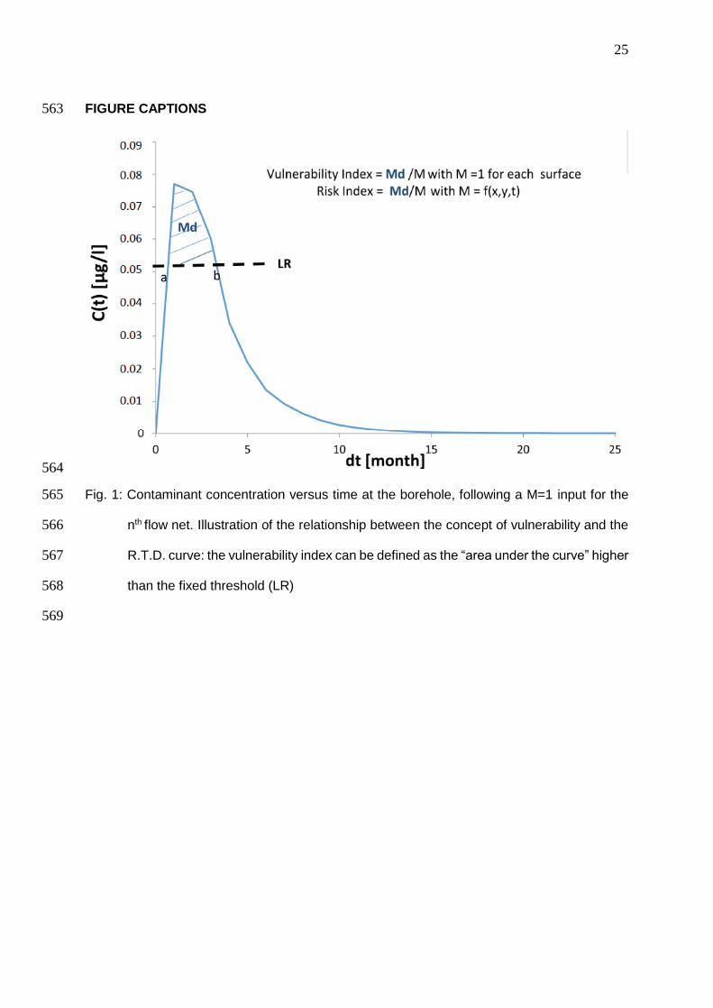
2.4. Analogy between RTD, vulnerability and risk indexes 186 The equivalent RTD for each flow net represents the mass arriving at the borehole for an 187
injected mass equal to 1. Depending on the value of the equivalent parameters, and on the 188
discharge 𝑄n for the 𝑛th flow net, the concentrations obtained make it possible to identify flow 189
nets showing concentrations higher than a threshold (LR) represented by the dashed line in 190
Fig. 1 while other flow nets present concentrations below the threshold. The spatialized grid of 191
equivalent parameters locates the surfaces which contribute to the over-concentration 192
measured at the groundwater borehole, making it possible to prioritize the various surfaces in 193
terms of borehole vulnerability and/or risk. 194
Using datasets of 𝑀 values, the specific risk index (𝐼) is defined as the rate between the mass 195
above the threshold 𝑀d (Fig. 1) and the mass flowing under the roots 𝑀. (equation 16). 196
I = Md
M=
∫ [E(t) M
Qn-LR]dt
b
a
M (Equation 11) 197
The boundaries 𝑎 and 𝑏 are defined in Fig 1 as the intercepts between the 𝐶(𝑡) curve and the 198
fixed threshold. So, the specific risk index 𝐼 is defined as the percentage of the applied 199
contaminant mass which will reach the borehole above a given threshold. If 𝑀=1 for the entire 200
watershed and the threshold has a low value, then equation 11 becomes an intrinsic 201
vulnerability index. 202
9
203
3. Study site and data 204
The proposed model was tested on the Val d’Orléans karstic system, which has a wide range 205
of flow velocities. This section presents the dataset required to apply the proposed 206
methodology, and the various existing ways to compile this database. 207
208
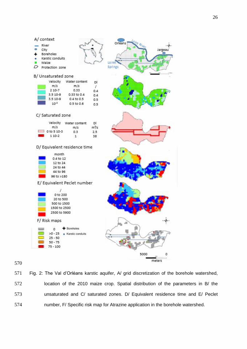
3.1. The Val d’Orléans 209 The Val d’Orléans is located southeast of Orléans city, in the alluvial plain of the Loire river 210
which corresponds to a depression of the main river bed. The length of this alluvial plain is 211
about 40 km and its maximum width reaches 7 km in its central part (Fig. 2). 212
3.1.1. Pedology 213
Inside the protection zone (Fig.2A), clays In soil represent about 0 to 250 g/kg. The sand 214
contents in silt (100 to 250 g/kg) and organic carbon (0 to 10 g/kg) are quite homogeneous 215
(BDAT-GISSOL-INRA, 2014). This database shows a low content of clays and sands in the 216
center and east of the perimeter and higher contents in the west zone. The values range 217
respectively from 0 to 100 g/kg and from 100 to 250 g/kg. 218
219
3.1.2. Geology 220
The geology in this sector results from a major and regular marine sedimentation 221
(transgression and regression phenomena), that started during the Trias and lasted until the 222
beginning of the Tertiary (Eocene). White chalk with flint and detritical formations constitute 223
the base of the geological formations of the Val d’Orléans. In the middle of the Tertiary 224
(Oligocene, Aquitanien), a sedimentation of lacustrine origin formed the limestones of Beauce, 225
interrupted with marly formations. In the second part of the Tertiary (Burdigalien), marls and 226
sands were deposited, before being covered by fluvial (Quaternary) alluviums of the Loire 227
(Auterives et al. 2014). For this study, only the sedimentary formations of lacustrine origin 228
10
which began during the Oligocene were of interest because it is the main aquifer. A karstic 229
network developed in the Beauce limestones, generally captive, either under the alluvial 230
formation or under the Burdigalien marls. A probability map of the karstic network was 231
proposed by Auterives et al., 2014. 232
This karstic network is supplied by surface water coming from the Loire river which infiltrates 233
at point sources (Albéric, 2004) in the area of Jargeau (Fig.2A) and by diffuse infiltration 234
through the alluvial plain located mainly in the river bed. Some of these karstic conduits outflow 235
downstream the Val d’Orléans where springs contribute to the establishment of the Loiret river 236
(Lepiller, 2006). Three drinking water boreholes are located within or close to the karstic 237
network (Fig. 2A). Based on the water quality data (isotopes and major elements) of the Loire 238
water, the local surface waters and the Loiret spring waters, Joigneaux (2011) revealed that 239
80% of the Loiret spring waters are composed of Loire water, the remainder being local surface 240
waters. Mixing is controlled by the hydrological conditions of the Loire river. 241
The groundwater vulnerability to diffuse agricultural pollution was estimated in the protection 242
zone of the three boreholes (Fig.2A). 243
244
3.1.3. Water flux and contaminants below the root zone 245
The discharge values 𝑄 arise from the hydrological balance. This assessment was made by 246
various authors such as Chéry (1983), Livrozet (1984), Lepiller (2006), Lelong and Jozja 247
(2008), Gutierrez and Binet (2010). Three different flow values were considered according to 248
three hydrological scenarios. These three scenarios represent the minimal, maximal and 249
average flows that transit through the system. The minimal flow can be estimated from the 250
lowest contribution of the flow from the Loire river and the lowest contribution of impluvium in 251
the total hydrological balance assessment. The minimal value of the contribution of the river 252
Loire loss was estimated at 5 m3/s (Martin and Noyer, 2003; Gutierrez and Binet, 2010), 253
whereas the lowest flow from the impluvium calculated by MACRO (Larsbo and Jarvis, 2003) 254
11
and calibrated for the Val d’Orleans is 0.100 m/year (Footways/Geo-Hyd, 2013). Thus, the 255
minimal contribution in water supplied to the system was estimated at 186.106 m3/year. 15% 256
of the water comes from diffuse infiltration. 257
Concerning the average flow, the volume of the Loire loss to the Val d’Orléans aquifer, for an 258
average year, was estimated by hydrological balance at 363.106 m3/year. The results of 259
models that estimate the effective rain, stemming from the impluvium, suggested a flow of 260
0.191 m/year (Joigneaux et al., 2011). The average flow transiting through the system is 261
estimated to be 423.106 m3/year. Here again, 15% of the water comes from diffuse infiltration. 262
The proposed RTD model was tested and calibrated for the application of atrazine, which was 263
sprayed between 1960 and 2003 on the maize crops. The reason for this choice is the 264
quantitative availability of analyses done on the three Val d’Orléans boreholes, which revealed 265
the presence of atrazine from the 1990s to 2004, showing, with a quarterly sampling frequency, 266
an erratic response with values ranging from 0 to 0.3 µg/L. Atrazine concentration in the Loire 267
river has been below the detection limit since the beginning of the century. In the 1990s, 268
concentrations reached 0.3 µg/L (Joigneaux, 2011). It is considered that the totality of the 269
atrazine concentration analysed at the three Val d’Orléans boreholes comes from diffuse 270
infiltration through the alluvial plain. The Loire river dilutes the fluxes. 271
The localization of the maize crops was mapped in 2010 and was assumed to be constant 272
through time (Fig. 2A). The atrazine masses injected during more than 40 years were 273
estimated from the history of agricultural practices recorded in various ways, such as 274
questionnaires collected by agricultural associations. Atrazine was applied by spraying, 275
generally made once a year, in April. The quantities of atrazine applied decreased over time, 276
(2.5 kg/ha/year in the 70th, 1.5 in the 80th, 1 betwwen 1991 to 1998, 0.75 in 1999 and 2000 and 277
0.5 betwwen 2000 to 2003) due to increasing constraints on the use of this herbicide, until it 278
was banned in 2003. Some studies show that pesticides such as atrazine can have an export 279
percentage up to 4 to 207 5% (Flury, 1996). Naturally, these ranges of values vary according 280
12
to the geo-hydro- morphological context of the site, but are mostly between 0.1 to 3% 281
(Wauchope, 1978; Flury, 1996; Voltz and Louchart, 2001). 282
283
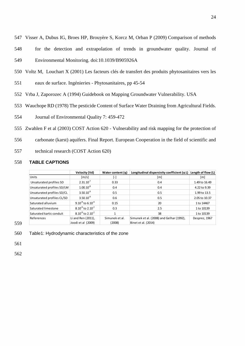
3.2. Field data for RTD estimation 284 Establishing the RTD requires data concerning the hydrodynamic characteristics of the aquifer 285
(Table 1). Each hydrodynamic parameter is attributed to each surface of the grid area (250 m 286
by 250 m, Fig. 2A). 287
The hydrodynamic characteristics of the unsaturated zone (UZ) were attributed according to 288
the lithology of the four profiles already defined (sand (SD), sand and limestone (SD/LM), sand 289
and clay (SD/CL) and clay and sand (CL/SD)). The length of flows are known from the 290
topographic elevation nimus the aquifer water head (Desprez in 1967). 291
In the saturated zone (Table 1), 2000 borehole logs were analysed. Alluvium, limestone and 292
karstified limestones were observed in the area (Auterives et al. 2014). In a saturated context, 293
the water content is equal to the porosity. 294
3.2.3. Atrazine in groundwater 295
Estimating the specific vulnerability requires knowledge of the specific behaviour of the studied 296
contaminants. For atrazine, a 10-year database is available, with more than 110 297
measurements. The atrazine degradation rate is known to be 0.4 [month-1] (IUPAC, 2013) and 298
rate of infiltration (𝑎) was estimated at about 0.05 (Kladivko et al., 1991). 299
300
3.3. Parametric tests on the “Val d’orléans” dataset 301 Uncertainty on the parameterization was explored by calculating various RTDs to assess the 302
impact of parameterization on the results. Before estimating the vulnerability mapping with the 303
RTD model, various parameter values were tested to observe the variability of the RTD. Here, 304
three tests concerning the unsaturated zone (UZ) are presented, as this uncertainty accounts 305
for the strongest error source in the calculation. The parametric tests presented will focus on 306
the UZ profiles spatialisation. Three models are presented in the Results section: 307

13
1. RTD_T1: For this scenario, it was considered that the UZ consisted of only one filtering 308
facies of sand (Profile SD) and no vertical karstic conduits. 309
2. RTD_T2: This configuration corresponds to the results of the spatial analysis of the 310
UZ profiles (best fit). 311
3. RTD_T3: This scenario uses the same hydrodynamic characteristics as T1 but adds 312
34 vertical karstic conduits, positioned according to the karstic network and a database 313
cavity, assuming that not all the vertical conduits are necessarily known. 314
4. Results 315
4.1. Equivalent Peclet numbers and average residence times 316 The spatial distributions of the hydrodynamic parameters used for the calculation of the 317
equivalent parameters and the intermediate calculations for RTD are presented in Fig. 2B. The 318
data concern the four types of profiles (Table1) and the limestone karst aquifer layer in the 319
saturated zone. The alluvium aquifer located above the limestone aquifer is not shown in Fig. 320
2B but was nevertheless taken into account in the calculation of the equivalent parameters. 321
The Fig. 2B and C shows the spatialized values (𝑉𝑑, 𝐿, , 𝑛𝑒 and ) from the UZ and SZ layers. 322
The second column gives the equivalent parameters (average residence times and equivalent 323
Peclet numbers) for the 𝑛 flow nets starting from the n grid cells and determined by equations 324
10 and 12. 325
4.2. RTD Calculations 326 The time discretization unit selected for contamimant transport was one month. This is 327
consistent with the assumption of steady-state conditions for the hydrology. 328
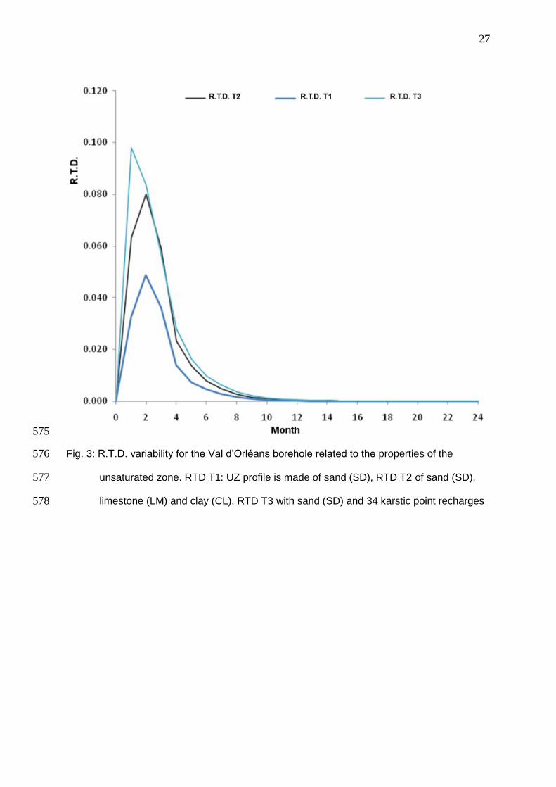
Fig. 2D shows the residence time distribution calculated from equation 13. The three scenarios 329
illustrate the variability of the results when parameters are varied in the unsaturated zone. The 330
parameters described in Table 1 correspond to the RTD_2 scenario. In this highly karstified 331
area, the residence times are short, less than 12 months, and the average residence time is 332
14
about 2 - 4 months. The two extreme cases (Fig. 3) show that the intensity of the concentration 333
peak can be twice as high in a karstic system compared to sand. 334
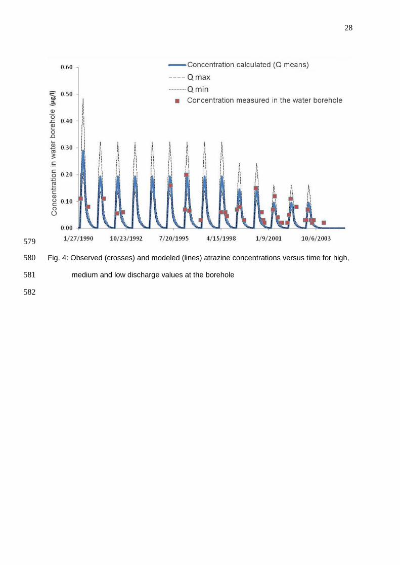
4.3. Concentration calculated at the water borehole by the RTD model 335 336
Figure 4 shows the concentration at the water borehole calculated by the RTD model. The 337
average flow reproduces the maximum groundwater concentrations in atrazine at the borehole. 338
The Nash-Sutcliffe coefficient was determined for the period 1990 to 2005. The value reaches 339
0.70. 340
341
4.4. Vulnerability and risk mapping 342 A vulnerability map can be computed, considering that each flow net receives a contaminant 343
mass 𝑀=1. The vulnerability can be estimated by prioritizing all the calculated RTDs (equation 344
16). Combining the vulnerability map with a hazard map (Fig. 2E) gives a risk map for atrazine 345
in the watershed. The results obtained are scaled on a range from 0 to 100. 346
Compared to traditional vulnerability mapping, this approach adds the notion of hydraulic 347
distance to from the borehole. Surfaces with a high index (in red) are not spatially the closest 348
to the borehole. 349
350
5.Discussion 351
352
The Nash-Sutcliffe coefficient suggests that the implementation of the equations, the 353
parameterization and the strong hypothesis proposed in the RTD model seem acceptable 354
for a risk assessment approach. 355
Concerning the mass of Atrazine applied on the field, the survey and the coefficient 356
used to evaluate the loss in organic soil give results in terms of water concentration at the 357
15
borehole in the same order of magnitude as the concentrations observed. The range of 358
uncertainty on the discharge (Q) and on Atrazine input (M) means that one can 359
compensate the other, and with the given data, it is difficult to determine where the 360
greatest source of error in our calculation lies. The uncertainty on the vertical conduit 361
location is a key parameter for a relevant vulnerability assessment. 362
The range of equivalent Peclet numbers and average residence times found for this 363
aquifer is wide. That is why a karst system was chosen to test this model. 364
The hydrology was assumed to be steady state. Although many authors point out that 365
water exchange between conduits and the surrounding rock drives the water quality at the 366
karstic outlet (Charmoille et al., 2009), this strong hypothesis was made for large time 367
steps, such as months or years. In these conditions, it is preferable to describe the average 368
behaviour of the system, which is easier to use for risk assessment. High or low water 369
stages can be estimated from the extreme discharge values (Fig.3). 370
Concerning the contaminant transport, the progressive decrease in atrazine concentration 371
observed at the borehole is correctly described by the model and corresponds to the decrease 372
in the quantites of atrazine applied to the maize crops (Table 1). The apparently erratic 373
distribution of the atrazine concentrations observed is explained by the pulses of atrazine 374
occurring 2 or 3 months after the injection periods. These results help to rationalize sampling 375
campaigns and to ensure a better management of water resources. 376
No storage was observed and advective flow control was observed in this highly transitive 377
system. However, a temporal shift of a few weeks (X axis) can be observed. The calculated 378
concentrations appear before the observed ones. We hypothesize that the origin of this 379
phenomenon is the uncertainty concerning the exact period of application. In our case, 380
atrazine application was considered to occur once a year, in April, but in reality applications 381
may have varied depending on the weather conditions. 382
16
The RTD model, based on literature datasets, made it possible to estimate a specific 383
vulnerability, which can then be validated by field data. Fig. 2E can be validated by time 384
series of contaminants observed in the water supply. There is no single solution that can fit 385
the concentration time series at the borehole. While many spatial distributions can lead to 386
the same lumped parameters, the advantage of the proposed approach is that it can test 387
whether the working hypotheses are sustainable. This is an improvement over the usual 388
method of vulnerability and risk assessment, and avoids the use of numerical groundwater 389
flow models that are generally over-parametrized. 390
391
6. Conclusions 392
The specific vulnerability index locates the potential source of groundwater quality 393
deterioration, but most assessment methods are qualitative. The Residence Time Distribution 394
model can address temporal and transient aspects of contaminant spreading and represent 395
them in a semi-quantitative manner. Such an approach makes it possible to establish a spatial 396
risk or vulnerability indexes validated by water quality changes at the borehole. The dataset 397
used in this method is commonly found in vulnerability studies. By using equivalent parameters 398
to take the characteristics of each layer into consideration, the spatial complexity of the 399
watershed can be reduced to an impulse response. The method based on the probability 400
distribution of residence times is a semi-objective method that can help groundwater managers 401
and decision-makers based on a physical approach to vulnerability assessment. The risk 402
mapped with this methodology gives the opportunity to test the efficiency of land practice 403
scenarios on the quality of the groundwater catchments. 404
405
Acknowledgements 406
This work is part of the PhD project supported by GEO-HYD (Antea members) and a national 407
grant from the National Research and Technology Association (ANRT – CIFRE). 408

17
The database used was made available by the INSU/CNRS national observatory of karstic 409
aquifers, SNO KARST. 410
411
18
References 412
Albéric P (2004) River backflooding into a karst resurgence (Loiret, France). Journal of 413
Hydrology 286: 194-202. 414
Aller L, Bennett T, Lehr JH, Petty RJ, Hackett G (1987) DRASTIC: a standardized system for 415
evaluating groundwater pollution potential using hydrogeological settings. US 416
Environmental Protection Agency. Washington, DC, USA. 417
Andersen L, Gosk E (1987) Applicability of vulnerability maps: Vulnerability of soil and 418
groundwater to pollutants, Proceedings and Information. TNO Committee on Hydrological 419
Research 28: 321-332 420
Aris R (1959) On the dispersion of a solute by diffusion, convection and exchange between 421
phases. Chemical reaction Engineering, doi: A252 422
Auterives C, Binet S, Albéric P (2014) Inferred conduit network geometry from geological 423
evidences and water-head in a fluvio-karstic system (Val d’Orleans, France). Environment 424
Earth Sciences. doi: 10.1007/978-3-319-06139-9_3 425
Bakalowicz M (2005) Karst groundwater: a challenge for new resources. Hydrogeology Journal. 426
doi: 10.1007/s10040-004-0402-9 427
Barry DA, Parker JC (1987) Approximations for solute transport through porous media with flow 428
transverse to layering. Transport in porous media, 2: 65-82 429
BDAT-GISSOL-INRA (2014). http://www.gissol.fr/programme/bdat/bdat.php. Accessed 10 430
December 2014 431
Beltman WHJ, Boesten JJTI, Van der Zee SEATM (1994) Analytical modelling of pesticide 432
transport from the soil surface to a drinking water well. Journal of Hydrology 169: 209-228 433
19
Binet S, Motellica M, Touze S, Bru K, Klinka T (2014) Water and Acrylamide monomer transfer 434
rates from a settling basin to groundwaters. Environmental Science and Pollution Research. 435
doi: 10.1007/s001090000086 436
Brouyère S (2001) Modelling of dual porosity media: comparison of different techniques and 437
evaluation on the impact on plume transport simulations. PhD Thesis Liège University 438
Chéry J (1983) Etude hydrochimique d’un aquifère karstique alimenté par perte de cours d’eau 439
(La Loire): Le système des calcaires de Beauce sous le Val d’Orléans. PhD Thesis Orléans 440
University 441
Civita M, De Maio M (2004) Assessing and mapping groundwater vulnerability to contamination: 442
The Italian “combined” approach. Geofisica Internacional 4: 513-532 443
Charmoille A, Binet S, Bertrand C, Guglielmi Y, Mudry J (2009) Hydraulic interactions between 444
fractures and bedding planes in a carbonate aquifer studied by means of experimentally 445
induced water-table fluctuations Coaraze experimental site, southeastern France. 446
Hydrogeology journal 17: 1607-1616 447
Desprez N (1967) Inventaire et étude hydrogéologique du Val d’Orléans. Rapport BRGM D-448
SGR-67-A21 449
Doerfliger N, Jeannin PY, Zwahlen F (1999) Water vulnerability assessment in karst 450
environments: a new method of defining protection areas using a multi-attribute approach 451
and GIS tools (EPIK method). Environmental Geology 39: 165-176 452
Escolero OA, Marin LE, Steinich B, Pacheco AJ, Cabrera SA, Alcocer J, (2002) Development 453
of a Protection Strategy of Karst Limestone Aquifers: The Merida Yucatan, Mexico Case 454
Study. Water Resour Manag 16: 351–367 455
20
Fernandez GP, Chescheir GM, Skaggs RW, Amatya DM (2006) DRAINMOD – GIS: A lumped 456
parameter watershed scale drainage and water quality model. Agricultural Water 457
Management. doi: 10.1016/j.agwat.2005.03.004 458
Flury M (1996) Experimental evidence of transport of pesticides through field soils - A review. 459
Journal of Environmental Quality 25: 25-45 460
Footways/Géo-Hyd (2013) Application Phyto’Scope au Val d’Orléans: Outils d’évaluation du 461
transfert des produits phytosanitaires de leurs zones d’application vers les eaux de surface et 462
les eaux souterraines 463
Gelhar LW (1992) A critical review of data on field-Scale Dispersion in Aquifers. Water 464
resources research 7: 1955-1974 465
Goldscheider N, Hötzl H, Fries W, Jordan P (2001) Validation of a vulnerability map (EPIK) 466
with tracer tests. 7th Conference on Limestone Hydrology and Fissured Media. Sci.Tech 467
Environ Mém. 13: 167-170 468
Goldscheider N, Popescu C (2003) Vulnerability and risk mapping for the protection of carbonate 469
(karst) aquifer. European commission Directorate - General for Research, pp 320 470
Gutierrez A, Binet S (2010) La Loire souterraine: circulations karstiques dans le Val d’Orléans. 471
Géosciences 12 : 42-53 472
Holman IP, Palmer RC, Bellamy PH, Hollis JM (2005) Validation of an intrinsic groundwater 473
pollution vulnerability methodology using a national nitrate database. Journal of Hydrology. 474
doi: 10.1007/s10040-005-0439-4 475
IUPAC (2013) Global availability of information on agrochemicals. University of Hertfordshire. 476
http://sitem.herts.ac.uk/aeru/footprint/es/Reports/43.htm. Accessed 10 April 2013 477
21
Jeannin PY, Cornaton F, Zwahlen F, & Perrochet P (2001) VULK: a tool for intrinsic 478
vulnerability assessment and validation. 7th Conference on Limestone. Hydrology and 479
Fissured Media, pp 185-190 480
Joigneaux E (2011) Etat qualitatif des eaux de la nappe du Val d’Orléans; Impact du changement 481
climatique et gestion durable de la ressource. PhD Thesis Orléans University 482
Joigneaux E, Albéric P, Pauwels H, Pagé C, Terray L, Bruand A (2011) Impact of climate change 483
on groundwater point discharge: backflooding of karstic springs (Loiret, France). Hydrol. 484
Earth Syst. Sci. 15: 2459-2470 485
Joodi AS, Sizaret S, Binet S, Bruand A, Alberic P, Lepiller M (2009) Development of a Darcy-486
Brinkman model to simulate water flow and tracer transport in a heterogeneous karstic aquifer 487
(Val d’Orléans, France). Hydrogeology journal 18: 295-309 488
Jurgens BC, Böhlke JK, Eberts SM (2012) Tracer LPM (Version 1): An Excel ® workbook for 489
interpreting groundwater age distributions from environmental tracer data. US Geological 490
Survey Techniques and Methods Report 4-F3, USA 491
Jury A (1982) Simulation of solute transport using a transfer function model. Water Resources 492
Research 2: 363-368 493
Kladivko EJ, Van Scoyoc GE, Monke EJ, Oates KM, Pask W (1991) Pesticide and nutrient 494
movement into subsurface tile drains on a silt loam soil in Indiana. Journal of Environmental 495
Quality 20: 264-270 496
Kreft A, Zuber A (1978) On the physical meaning of the dispersion equation and its solutions for 497
different initial and boundary conditions. Chemical Engineering Science 33: 1471-1480 498
Larsbo M, Jarvis N (2003) A model of water flow and solute transport in macroporous soil. 499
Technical description. Studies in the biogeophysical Environment. Swedish 500
22
Lasserre F, Razack M, Banton O (1999) A GIS-linked model for the assessment of nitrate 501
contamination in groundwater. Journal of Hydrology 224: 81-90 502
Ledoux E (2003) Modèles mathématiques en hydrogéologie. Document du Centre d’Information 503
Géologique Ecole Nationale Supérieur des Mines de Paris, Paris 504
Lelong F, Jojza N (2008) Fonctionnement du système karstique du Val d’Orléans: les acquis, les 505
interrogations. CFH - Colloque hydrogéologie karst au travers des travaux de Michel 506
Lepiller, Orléans 507
Lepiller M (2006) Le Val d’Orléans. Aquifère et eaux souterraines en France (BRGM), pp 508
200-214 509
Levenspiel O (1962) Chemical reaction engineering. New York 510
Li C, Ren L (2011) Estimation of unsaturated soil hydraulic parameters using the ensemble 511
kalman filter. Vadoze Zone Journal 10: 1205-1227 512
Livrozet E (1984) Influence des apports de la Loire sur la qualité bactériologique et chimique de 513
l’aquifère karstique du Val d’Orléans. PhD Thesis Orléans University 514
Maloszewski P Zuber A (1982) Determining the turnover time of groundwater systems with the 515
aid of environmental tracers – 1. Models and their applicability. Journal of hydrology 57: 516
207-231 517
Martin JC, Noyer ML (2003) Caractérisation du risque d’inondation par remontée de nappe sur 518
le Val d’Orléans. BRGM, Orléans 519
Molénat J, Davy P, Gascuel-Odoux C, Durand P (1999) Study of three subsurface hydrologic 520
systems based on spectral and cross-spectral analysis of time series. Journal of Hydrology 521
222: 152-164 522
Nash JE, Sutcliffe JV (1970) River flow forecasting through conceptual models part I - A 523
discussion of principles. Journal of hydrology 10: 282-290 524
23
Neukum C, Hötzl H, Himmelsbach T (2008) Validation of vulnerability mapping methods by 525
field investigations and numerical modelling. Hydrogeology Journal. doi:10.1007/s10040-526
007-0249-y 527
Panagopoulos GP, Antonakos AK, Lambrakis NJ (2006) Optimization of the DRASTIC method 528
for groundwater vulnerability assessment via the use of simple statistical methods and GIS. 529
Hydrogeology Journal 14: 894-911 530
Petelet-Giraud E, Doerfliger N, Crochet P (2001) RISKE: Méthode d’évaluation multicritère de 531
la cartographie de la vulnérabilité des aquifères karstiques. Application aux systèmes des 532
Fontanilles et Cent-Fonts (Hérault, France). Hydrogéologie 4: 71-88 533
Plummer R, de Loë R, Armitage D, (2012) A Systematic Review of Water Vulnerability 534
Assessment Tools. Water Resour. Manag. 26: 4327–4346 535
Sadek MA, Abd El-Samie SG (2001) Pollution vulnerability of the Quaternary aquifer near Cairo, 536
Egypt, as indicated by isotopes and hydrochemistry. Hydrogeology Journal. doi: 537
10.1007/s100400100125 538
Schwientek P, Maloszewski P, Einsiedl F (2009) Effect of the unsaturated zone thickness on the 539
distribution of water mean transit times in a porous aquifer. Journal of Hydrology 373: 540
516-526 541
Šimůnek J, Šejna M, Sakai M, Van Genuchten M Th. (2008) The HYDRUS-1D Software 542
Package for Simulating the One-Dimensional Movement of Water, Heat, and Multiple 543
Solutes in Variably-Saturated Media. Riverside, California 544
Srinivasan R, Arnold JG (1994) Integration of basin-scale water quality model with GIS. Water 545
resources 30: 453-462 546
24
Visser A, Dubus IG, Broes HP, Brouyère S, Korcz M, Orban P (2009) Comparison of methods 547
for the detection and extrapolation of trends in groundwater quality. Journal of 548
Environmental Monitoring. doi:10.1039/B905926A 549
Voltz M, Louchart X (2001) Les facteurs clés de transfert des produits phytosanitaires vers les 550
eaux de surface. Ingénieries - Phytosanitaires, pp 45-54 551
Vrba J, Zaporozec A (1994) Guidebook on Mapping Groundwater Vulnerability. USA 552
Wauchope RD (1978) The pesticide Content of Surface Water Draining from Agricultural Fields. 553
Journal of Environmental Quality 7: 459-472 554
Zwahlen F et al (2003) COST Action 620 - Vulnerability and risk mapping for the protection of 555
carbonate (karst) aquifers. Final Report. European Cooperation in the field of scientific and 556
technical research (COST Action 620) 557
TABLE CAPTIONS 558
559
Table1: Hydrodynamic characteristics of the zone 560
561
562
Velocity (Vd) Water content (q) Longitudinal dispersivity coefficient (L) Length of flow (L)
Units [m/s] [-] [m] [m]
Unsaturated profiles SD 2.31.10-7 0.33 0.4 1.49 to 16.49
Unsaturated profiles SD/LM 1.00.10-8 0.4 0.4 4.22 to 9.39
Unsaturated profiles SD/CL 3.50.10-9 0.5 0.5 1.99 to 13.5
Unsaturated profiles CL/SD 3.50.10-9 0.6 0.5 2.05 to 10.37
Saturated alluvium 9.10-8 to 6.10-4 0.15 20 1 to 14467
Saturated limestone 8.10-8 to 2.10-2 0.3 2.5 1 to 10139
Saturated kartic conduit 8.10-8 to 2.10-2 1 38 1 to 10139
References Li and Ren (2011),
Joodi et al (2009)
Simunek et al.
(2008)
Simunek et al. (2008) and Gelhar (1992),
Binet et al. (2014)
Desprez, 1967
25
FIGURE CAPTIONS 563
564
Fig. 1: Contaminant concentration versus time at the borehole, following a M=1 input for the 565
nth flow net. Illustration of the relationship between the concept of vulnerability and the 566
R.T.D. curve: the vulnerability index can be defined as the “area under the curve” higher 567
than the fixed threshold (LR) 568
569
26
570
Fig. 2: The Val d’Orléans karstic aquifer, A/ grid discretization of the borehole watershed, 571
location of the 2010 maize crop. Spatial distribution of the parameters in B/ the 572
unsaturated and C/ saturated zones. D/ Equivalent residence time and E/ Peclet 573
number, F/ Specific risk map for Atrazine application in the borehole watershed. 574
27
575
Fig. 3: R.T.D. variability for the Val d’Orléans borehole related to the properties of the 576
unsaturated zone. RTD T1: UZ profile is made of sand (SD), RTD T2 of sand (SD), 577
limestone (LM) and clay (CL), RTD T3 with sand (SD) and 34 karstic point recharges 578
28
579
Fig. 4: Observed (crosses) and modeled (lines) atrazine concentrations versus time for high, 580
medium and low discharge values at the borehole 581
582


![MAPPING SPATIAL DISTRIBUTION OF WATER QUALITY …environmental fields [10, 11, 12]. In groundwater, GIS is commonly used for site suitability analyses, estimation of groundwater vulnerability](https://static.fdocuments.us/doc/165x107/600759dadc5fc24ddd424c5c/mapping-spatial-distribution-of-water-quality-environmental-fields-10-11-12.jpg)