SLAC-PUB-5756 February 1992 (A)

GROUND MOTION -AN INTRODUCTION FOR ACCELERATOR BUILDERS*

G.E.Fischer Stanford Linear Accelerator Center, Stanford, CA 94309 U.S.A.

Abstract In this seminar we will review some of the characteristics of the major classes of ground motion in order to determine whether their effects must be considered or place fundamental limits on the siting and/or design of modem storage rings and linear colliders. The classes discussed range in frequency content from tidal deformation and tectonic motions through earthquakes and microseisms. Countermeasures currently available are briefly discussed.

1. INTRODUCTION

In not so many years from today we will be entering’the twenty-first century and during this time some of us may also be entering (or be pushed into it, kicking and screaming) what I like to call the micron world of accelerator alignment. Instead of

&lking to you about what I was originally supposed to talk to you about -- how to do metrology in this world -- I thought it might be worthwhile to spend the next hour examining some of the features- of t.his intolerant world, in which steel appears to behave like butter and you dare not turn the room lights on, so that when we meet it we will, perhaps, have taken some of the necessary precautions and thus not be too surprised.

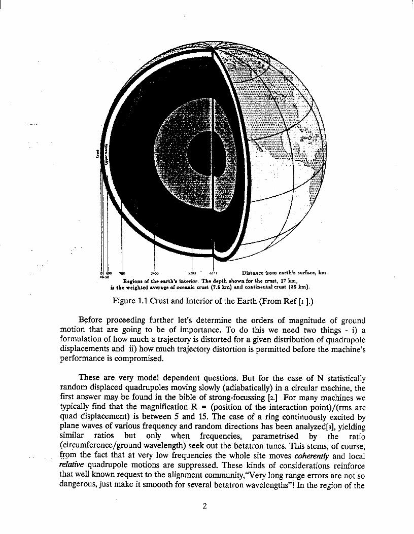
In line with the CERN Accelerator School Seminar format I feel encouraged also to visit subjects that are not related to accelerators per se. These visits will need to be fleeting because the study of the Earth Sciences is carried out far more extensively than studies in our own field. I will therefore try to provide you with an appropriate literature resource. But if there is one thing I would like to have you carry away from todays meeting, it would be the firm realization that the surface of the earth, this thin, elastic, wrinkled, and in places broken skin, floating on the gooey upper mantle (see Fig.1) in which we wish to construct well aligned accelerators, is anything but Terra Firma. It is constantly subject to a variety of external and internal forces, It is constantly in motion.

In discussing motion it seems useful to pose our problems in sensible coordinate systems. That is “What or who is moving with respect to whom?” For example, we need not be as elaborate when discussing say the vibration isolation of an electron or tunneling microscope from its foundation than we need be ‘in mounting an

-~ ** ‘interferometric gravitational wave detector (see Fig.2). In the accelerator world it is often useful to distinguish between local regions (say within a few betatron wavelengths) and the coordinate system that describes the global features of the trajectory. *Work suppork-d by the Department of Energy, contract DE-AC03-76SFOO515

Invited talk presented at the CERN Accelerator School: Course on Magnetic Measurement and Alignment, Montreux, Switzerland, March 16-20, 1992

3

4.& J s&o Distance from earth’s surface, km

Regionr of the earth’s interior. The depth shown for the crust, 17 km, t the weighted average of ocemic cruet (7.6 km) and continental crust (35 km).

Figure 1.1 Crust and Interior of the Earth (From Ref [l I.)

Before proceeding further let’s determine the orders of magnitude of ground motion that are going to be of importance. To do this we need two things - i) a formulation of how much a trajectory is distorted for a given distribution of quadrupole displacements and ii) how much trajectory distortion is permitted before the machine’s performance is compromised.

These are very model dependent questions. But for the case of N statistically random displaced quadrupoles moving slowly (adiabatically) in a circular machine, the first answer may be found in the bible of strong-focussing [2.] For many machines we typically find that the magnification R = (position of the interaction point)/(rms arc quad displacement) is between 5 and 15. The case of a ring continuously excited by plane waves of various frequency and random directions has been analyzed[s], yielding similar ratios but only when frequencies, parametrised by the ratio (circumference/ground wavelength) seek out the betatron tunes. This stems, of course, from the fact that at very low frequencies the whole site moves cohere&y and local retie quadrupole motions are suppressed. These kinds of considerations reinforce that well known request to the alignment community,“Very long range errors are not so dangerous, just make it smoooth for several betatron wavelengths”! In the region of the

2

IP a another maxim exists. Since there is almost parallel to point focusing here, there is an almost one to one ratio between final lens motion and displacement of the beams at the IP. Again this will be a r&&e tolerance, for if both lenses sink the same amount, then both beams sink the same way and they remain in collision.

For these simple arguments, let us define loss of machine performance to occur when the beams begin to miss each other by say 10% of their beam size at the IP. In the SSC (Texas), the beam size is about 5 p (micrometers). To achieve the high luminosity required at the NLC (Next Linear Collider) in which beams are focussed to nanometers at the collision point, it has been estimated [4] that ground motions along

.- the linacs should be less than about 50 nm (rms). It is planned to use passive isolation to limit high frequency (5 to 50 Hz) jitter. Beam based feedback, limited by the sampling rate, is extensively employed below about 2 Hz to satisfy our requirements.

While it is beyond the scope of todays lecture to delve too deeply into the vibration countermeasures industry, it may be interesting to look at one of the most ambitious applications of this technology that I know of. It is shown in Fig.2 below.

7

Fig.2. Proposed full-scale Gravitational Wave Detector. (From Ref [s].)

A laser beam is used to measure the distance between two mirrors fixed to separate masses. The arms will stretch several kilometers from the central laboratory. When a gravitational wave passes the detector, the distance between the masses alters, leading to a change in the time it takes for the laser beam to return. The gravitational beam also affects the propagation of the light, that is it distorts the fabric of space-time, biit the two effects do not cancel each other out. In practice it is easier to measure the difference in time taken for light to travel in two different directions, at right angles: the gravitational wave makes one of these distances increase and the other diminish.

3

2. TIDAL DEFORMATIONS

The largest external forces on the earth are the gravitational attractions of the moon and sun which distort the its oblate spheroidal shape in various periodic ways, modifying the gravitational potential on the surface and producing the tides.[6] . Already in 1876 Lord Kelvin pointed out that a non-rigid earth should suffer periodic radial excursions. By comparing long-period ocean tides with theory, G.H.Darwin (son of Charles Darwin) concluded in 1883 that the earths crust is rising and falling with amplitudes approximately l/3 that of the oceans that cover it.[7] The geometry of the mechanical arrangement is shown in Fig.3 below.

Fig.3. The Planes of Planetary Motion (From Ref.[s])

The gravitational attraction of either moon or sun is to produce two symmetric bulges on the surface of the earth as shown in the figure on the left below. But because the rotational axis of the earth is inclined to the lunar orbital plane an asymmetry is induced in the two tides that occur daily. The ellipticity of orbits introduces further periodicities resulting in a complex spectrum of 11 major and many minor components..

Sun or Moon

Moon

.* /

2.1 Effects of the tides

4

What, you may ask, does all this have to do with the precise alignment of future accelerators? Four measurable surveying quantities ( height, strain, tilt and the acceleration due to ‘gravity’ ) now depend on when in the day, month or year you measure them. 2.1.1 Height

The first of these will become important when the Global Positioning System (GPS)[9] method of locating surface monuments includes the local absolute vertical component, a quantity, measured with respect to the center of the earth that could vary by as much as 57 cm in 6 hours. 2.1.2 Strain

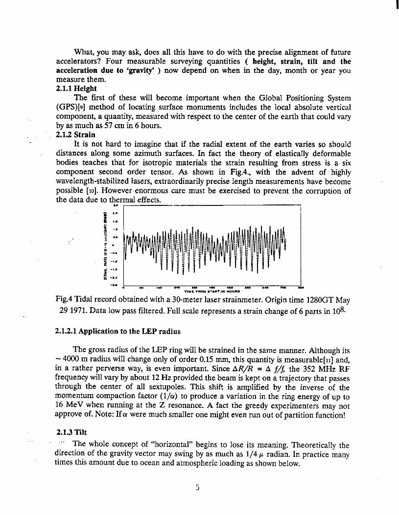
It is not hard to imagine that if the radial extent of the earth varies so should distances along some azimuth surfaces. In fact the theory of elastically deformable bodies teaches that for isotropic materials the strain resulting from stress is a six component second order tensor. As shown in Figd., with the advent of highly wavelength-stabilized lasers, extraordinarily precise length measurements have become possible [lo]. However enormous care must be exercised to prevent the corruption of the data due to thermal effects. a.0

Fig.4 Tidal record obtained with a 30-meter laser strainmeter. Origin time 1280GT May 29 1971. Data low pass filtered. Full scale represents a strain change of 6 parts in 108.

2.1.2.1 Application to the LEP radius

The gross radius of the LEP ring will be strained in the same manner. Although its - 4000 m radius will change only of order 0.15 mm, this quantity is measurable[n] and, in a rather perverse way, is even important. Since AR/R = A f/j the 352 MHz RF frequency will vary by about 12 Hz provided the beam is kept on a trajectory that passes through the center of all sextupoles. This shift is amplified by the inverse of the momentum compaction factor (l/a) to produce a variation in the ring energy of up to 16 MeV when running at the Z resonance. A fact the greedy experimenters may not approve of. Note: If ar were much smaller one might even run out of partition function!

2.1.3 Tilt The whole concept of “horizontal” begins to lose its meaning. Theoretically the

direction of the gravity vector may swing by as much as l/4 p radian. In practice many times this amount due to ocean and atmospheric loading as shown below.

5

Fig.5 A 100 hour record segment of two orthogonal tilt components showing their amplitudes and phase. Taken by mercury level in a deep gun gallery at the San

Francisco Presidio in 1969. (From Ref.[12])

.- 2.1.4 Variations in the magnitude of “gf9. All devices that are affected by gravity will experience periodic change. On the

rising and falling surface of the earth the fractional variations of “g” are of order 2.5 x lo-? That the combined changes in potential are all too real can be seen from the data below. Notice the similarity to Figure 4.

“T 50 )rgols

: + FORTNIGHTLY WAVE

4

HONTILY WAVE

,’

+I I-+ t 21 lunar transit

(24.8 hrs)

Fig.6. Stanford Station Tidal Gravity Record illustrating Monthly and Fortnightly Waves due to varying lunar orbital elliptic@ and declination respectively Ref 12.

I

If you take data over a long enough time you can Fourier analyze such data with remarkable precision as is shown in the next figure. Notice that the main contribution, the semi-diurnal moon component (M2) is 80 db above the noise power. Such data can be used, together with astronomical data, to provide very accurate predictions of the total gravitational tide potential. The coefficients of such series are published13 and permit anyone with a desktop computer to become an amateur tide chart&t. You may be amused to see an example of how it was done in Kaiser Wilhelm II’s time. Figure 8 depicts an analog computer, run by a 3/4 HP motor which sums the 11 major components and draws the resultant tide on a roll of chart paper. The device is located k-the marine museum in Bremerhavn. It’s quite clear the German Navy was not about to run aground on the sand banks of the North Sea. If all this is so predictable why worry? Unfortunately we must also account for the weather! And you all know how easy that is to do.

6

Figl7. Power spectrum of grahmeter signal in the 1 and 2 &%/day bands for an 18 month record at Pinon Flat, California. (From Ref[l4])

Fig.8 Mechanical Computer used to calculate the height of the tide. Circa 1907. Note the eleven wheels. (Marine Museum - Bremerhavn)

2;2 The Length of Day Problem

Now that we have touched the question of the oceans and winds we might just as well discuss their influence on that global mechanical issue: the speed of rotation.

7

Fortunately the astrophysicists have developed a remarkable tool to aid in the study. It is called Very Long Base Line Interferometry, VLBI for short. Consider the diagrams of Figure9.

Fig.9. VLBI observations can detect the time delay between the arrival of a quasar signal (so far away on the right that its emissions CiUl be considered plane waves when they arrive at the earth) at one radio telescope and its arrival at a second telescope. In this simplified illustration both telescopes are on the Equator. As the earth rotates, the time delay At follows a sinusoidal pattern. At the time T1 the signal arrives at telescope A first; at T2 it arrives at both telescopes simultaneously, and at T3 it arrives at telescope B first. At T4 the earth has completed one revolution, and the time delay has returned to its value at Tl; the interval from T1 to T4 is exactly one day, and with KBI it can be measured to within 0.1 millisecond. The amplitude of the time delay is proportional to the length of the baseline AB. (From Ref [IS])

Local times can be measured by hydrogen maser clocks.

Ale - :.

This extraordinary timing, which can be carried out over years, has been used the kinds of older astronomical observations shown in Fig.lO.on the next page.

to verify

s

.-

Fig.10. Length of Day Observations. All parts of the figure depict the

changes in the length of the day in parts per 108. Since there are 8.6 x 104 seconds in the day one can see from the upper

-4 I \ /

curve that over the past century, the days . 11111111111~1 I 1 1900

have become longer by about 2 1050 19xI ’

milliseconds. The linear shift is believed pfmhld

I I

to be due to tidal friction and effects of the last ice age. The positive and negative bumps ‘are believed due to core - mantle interactions. These changes of angular momentum must also have had an effect on the moon. Indeed due to this

I r I I I T I I I I I 1965 . ’ 1970 1975

coupling, the moon is also slowing down pwlrin1O

and its orbital distance from the earth is getting larger Could the moon have once c

1

been .part of the earth you ask?. I will leave this fascinating question for you, as students, to look up. 9.5

The middle part of the figure depicts changes in the length of day on a finer 0

time scale.. This data was obtained from the satellite LAGEOS. The fine structure is believed to be due to annual pattern changes in the east-west wind.

The pattern shown in the bottom part is --t--T-

said to be due to the weather. Does it t

appear to be predictable?

(Figure from Ref [S]) c / :&T

1 l’hly lJ4n 1999 1999

One other geophysical fact worth mentioning before we leave this subject[x] is that the earth’s axis of rotation does not remain fixed with respect to the earth’s surface. This angular wobble .( called the Chandler wobble after the American Astronomer who reported it first in 1891) currently has almost equal amplitudes east- west and north-south of about 0.3 arc seconds. That amounts to a radius at the north pole of about 4 meters. The vector appears to rotate counter-clockwise in roughly once a year. The source of the excitation is thought to be large earthquakes, but remains controversial.

9

3. TECTONIC MOTIONS AND CRUSTAL DEFORMATIONS

The general acceptance, in the late 1960’s, that we are all floating around the surface of the earth on large islands called tectonic plates has led to a revolution in the understanding of many of the geophysical manifestations, the sources of which were mysteries before that time. Plates in collision produce mountain ranges and earthquakes. The Pacific Plate moving north-west over a stationary hot plume is said to explain the distribution of the Hawaiian islands. The spreading of the Atlantic producing the ridge that runs through Iceland down the middle of the south Atlantic ocean separating South America from Africa are all examples of this understanding.

Let me take a moment to tell you a little story. I found myself, one day, on the sea coast of Brazil near Recife. A Portuguese speaking f=herman had just snagged a sea turtle. He threw it back. He explained, arms gesticulating, that it had probably returned by swimming all the way across the Atlantic, from an island off the coast of Africa about 3000 miles away. I didn’t believe this fish story either, until a few years ago when it was all explained to me. It seems this kind of turtle used to lay her eggs on an island just off the coast of Brazil to escape predators. Two hundred million years later, after the two continents dried apart, her species is still doing it, swimming slightly further each year. Did her kind exist so long ago?. Probably, because evidence of the Permian reptile Mesosaurus has been found on both continents.

Fig. 11. A piece of Pangea. The fit of the continents around the Atlantic Ocean&After Bullard et al. 1965) The best lit adjusted to the 500 fathom contour. Black areas represent overlap, shaded areas are gaps. The

arrows point to where Recife is today.

The gross boundaries of the worlds tectonic plates are shown in Fig.12. The manner in which intercontinental distances are changing is shown in Fig. 13. This figure is taken from data of the Crustal Dynamics Project sponsored by NASA whose mission is to further develop VLBI and Satellite Ranging techniques and, with the cooperation of many different countries, to implement global networks of stations.

3.1 SLR Techniques

.-

The LAGEOS satellite is a 60 cm diameter sphere, weighing 411 kilograms, which orbits the earth at an altitude of 6000 kilometers, passing round our planet in 3 hours 25 minutes. It surface is studded with 425 laser retro-reflectors. Ground stations transmit short intense pulses to the satellite whose orbit is very well known. The round trip time of flight is precisely measured permitting accurate determination of the station locations and baselines between them. The ground stations can be made relatively mobile. The task of processing of the data is a highly complex and time consuming effort requiring both expertise and computer resources including solving the orbital parameters of the satellite, making appropriate corrections for atmospheric delays, variations in the rotation of the Earth and tidal effects. Current capability for measuring relative motions over a 5 year period is better than lOmm/year. But sharpening this accuracy to lmm/y will take an enormous effort and research. Limitations exist in part in the ..hardware, errors in atmospheric delay (water vapor) as well as noise from local non-tectonic causes such as rainfall induced local ground inflation.

Higher accuracy drift rate measurements are very much desired for stations in California, where the complexity of the plate boundary, the number of individual blocks and faults, and the variable distribution of deformation make the picture far from simple. See for .example: the question of the “San Andreas Discrepancy, a mismatch between the rate and direction of horizontal slippage along the San Andreas Fault and the relative motion of the Pacific and North American plates[r7]

3.2 GPS Techniques

During the last half of the 1980’s, the civilian use of GPS has become the deformation geodeticists’ tool of choice[ls]. This may be particularly true for local networks, such as might be of used by accelerator builders. Originally conceived by the U.S. Department of Defense to permit any member of its personnel who had access to the requisite codes broadcast by the satellites, to ascertain in real time just where they are anywh on the surface of the earth to within about ten yards, it is now used in a great variety of ways never contemplated by the military. Civilian scientists have managed to use the radio signals to determine ZocaZ relaive position to centimeters or better. Quite suddenly, a large number of problems have become feasible to “small science”, in particular the very important determination of the compliance of individual fault zones. Moreover unlike the more traditional methods, both the vertical as well as the horizontal coordinates are treated at the same time, nor do the benchmarks have to be inter-visible should they be obscured by topography, buildings or haze.

11

f ;:c

.- .s

.- B t $1 -.,+:

i ~ ‘3 :

i .’ .

25 12

CJ j

I I .G

I

Y

-.

i- -

t q .’ c

1 1: TN

#.

t

‘I? 1

bta ---

3{ 1

-Y, I

D

\ ,

q,:i

y w

I

‘I Q

D ye& \

I E

fi “;

c? c &a,

zs c

0 .2 2;

J J

z z

r z

‘- 1

I =

b f

I >

~~1

-- 5

J L >a =.

‘_

::

2, s ‘3

..* Fig.12. Major Plates of the world. M

idoceanic ridges, at which plates move apart, are

represented by double lines. Trenches and other subduction zones are marked by lines

with teeth pointing down the descending slab. (Figure from Ref [l])

12

.Fipre 13. Rates of Plate m

otion (in mm

/years) between various worldwide sites as determ

ined by Satellite Ranging System (SLR) - LAG

EOS.

(From Ref

[19] and later NASA Tech.Note in 1988)

13

By the end of 1992 when the full complement of satellites is planned to be in orbit at least four will be visible simultaneously. Each satellite broadcasts a coded message that, by synchronization, gives the time at which the signal leaves the satellite as well as the satellites position as a function of time. The time of arrival of the signal is recorded at each earth station in terms of accurate and well synchronized clocks. The range is deduced from these observations. Ranging to two satellites places the receiver somewhere on the circle formed by the intersection of the two spheres centered on each satellite. Ranging to three satellites places the receiver at one of two points formed by the intersection of three spheres. The knowledge that the receiver is at the surface of the earth removes this last ambiguity. Acquiring the signal from the fourth satellite allows receiver clock offset to be determined. GPS is essentially a “two color system” in that signal propagation through the dispersive ionosphere is accounted for by using two frequencies (ie. 19 cm and 24 cm wavelength).

The trick employed to get r&ztive coordinates is to do interferometry on the carrier wave. Now it is very helpful to know the approximate coordinates since phase measurements are inherently ambiguous modulo 19 cm integer wavelength. GPS applied to our accelerator alignment needs, in 1986, the closing error of the Stanford Linear Collider (SLC) surface survey net of some 9 stations distributed over several kilometers was found to be about 2mm rms. Moreover the coordinates were in agreement with those found by the then current Electronic Distance Measuring (EDM) methods. While it is tempting to describe GPS in more detail, in particular with respect to the reduction of its errors, I recommend that you study the recent review quoted above because the application of GPS is a very fast moving field. One day accuracies of a few parts in 108 may become possible.

3.3 Monuments

As the demands for precision increase, so must our understanding of the forces that displace the local benchmarks of our networks. The surface soil is subject to swelling by rain water and thermal distortions due to temperature variation. Fig. 14 depicts a typically simple solution to such disturbances, a heavy concrete pillar going deep into the ground. Other solutions that transfer underground coordinates to the surface include the upside down pendulum adopted by CERN early in the construction of the PS [u)] and an extraordinary 24 meter deep interferometric device called the “Optical Anchor”[zi] at Pinyon Flat Observatory in California.

Speaking of thermal effects calls into mind a situation that occurred at SLAC when we were planning the alignment system[z] for the Final Focus Test Beam, a 50 GeV test transport system for some future linear collider designed to focus the beam to 60 run. The question was: “How much and how fast could the surface of the research yard, which is exposed to the weather, move transversely?” Nobody could come up with a plausible model. A measurement was clearly indicated. To reduce effects due to the atmosphere, EDM and later interferometer measurements were set up using an evacuated flight path. The continuously monitored coordinates moved back and forth daily by as much as 700 microns. The driving mechanism is shown in Fig. 15. The sun, as it heats up first the north side, pushes the yard south. In the afternoon the reverse occurs. We hope we have solved the problem by slicing the concrete in such a manner

14

so that these normally occurring themtoelastic defonnrdions are not transferred to the support footings of the beam which are anchored to the substratum miocene sandstone.

-- FFTD .-

Fig.15. Differential heating of the yard.

. . . . ...?.;.!: . *Tr*i;.;;*y.!.::$ ::!:+.:iz ? *.. ,* . 1,J>~*4&.3-+ * .

, ., ,,.,$y?+ ,,,,<j..::5 ’ .>.fj L’.. ,.I

.,;r.:; *‘- . ..%r*

Fig.16. The Earth’s Heat Engine Figure taken from the New York Times - Science Times section entitled “ Deep Plumes Shape Earth and Its Climate” Spring1991.

15

4. EARTHQUAKES

, Although the earthquake problem does not concern the accelerator builder in first order ( unless he or she happens to be unluc~ enough to be in the vicinity of the wrong kind of fault ) it nevertheless demands our attention because almost everything we know about the inside of the earth was derived from the study of these world shaking events. Nature has very conveniently provided us with a probe - sound through the ground - with which to peer into the depths. If we are able to decode its message (the computer is a marvellous tool for this) every time the worlds’ networks of seismic stations records an event, the earth is taking an auto-sonograph of itself. For this reason we must make a short digression at this point to briefly review how mechanical disturbances propagate, we must review the issue of the velocities of sound.

4.1 Sound Velocities

Consider for a moment that mathematical abstraction, the homogeneous, isotropic, perfectly elastic, semi-infinite medium. It can be shown[zs] that for the irrotational wave(the special case that occurs when the curl of the displacement vector is zero).and often called more loosely the compressional wave, longitudinal wave, P wave, or primary wave has a velocity:

(4.1)

in which k is the bulk modulus, ,Q the shear modulus and p the density.

For the special case in which the divergence of the displacement vector is zero, that is the medium is incompressible, we find the solenoidal wave, sometimes called the transverse wave, the shear wave or the secondary wave because its velocity:

cs = &P / P) must be slower. In general, both types are present, but notice that in a liquid or a gas, which have no shear strength, only pressure waves can be supported.

The quantities k and ,X can be combined to yield the more familiar Poisson’s Ratio (a) and Youngs Modulus (Y) by the relations:

0 = 3k - 2~ 6k + 2~ (4.3)

Y 9w

= p+3k = 3k(l - 20) = 2j.~(1 + o)

(4.4) Hence, knowing any two of the material constants permits calculation of the other two.

The velocity ratio C,/C, is also of interest. If for example, (T = l/4 , as is approximately true for many earth materials, then k = 5/& and C& = sqrt 3 = 1.73. Some numerical values for these rock and soil parameters are shown in the table below:

Table4.1.

.-

Material Granite Shale Lime- Miocene \ stone Sandstone

Cp 5-6 km/s 2.2 -6 3-7ooo’/s cs 2-3 km/s 0.81 -3 1-4000’/s k 3.OEll

dyne/cm* u 2Ell 0.51E6 nsi

1 D 1 2.7 1 I 1.91 I CJ 1 0.2-0.3 1 I I 0.15 0.35 I in

c,/c, 1.63-1.87 2.72 2.0 1.56 Y 7.3E6psi 1.2E6 psi

Austin Mexico Chalk[a] City 253Om/s do not 1219m/s even 2.OE6 psi think

0.46E6 nsi I about 2.16 I building

The values in the table are only meant as a guide. First, we have to recognize that as one descends from the surface, almost all materials are consolidated by the weight of the overburden, raising the density, the strengths and the velocities. The accelerator builder must measure these values at tunnel depth. For a more comprehensive treatment see Reference [u].

To demonstrate the difference of p and s wave velocities, examine a typical seismogram taken at SLAC on the day of the 1983 Coalinga Earthquake: Fig. 17 below.

MAIN EVENT M-5.9

26 SEC JULY 21, I 983 COALING A ,CALIFORNIA

LONG PERIOD INSTRUMENT SLAC 26 SEC fi: 230 KM

20-43-44 .

. AFTERSHOCK M,-4.7

Let us reconstruct the event knowing the answer. Coalinga is located just off the San Andreas fault about 230 krn to the south of SLAC. Assuming an average p wave velocity of 5 km/set, the first signal arrived 46 seconds after the initial main shock (top left of the recording). Letting the s wave travel through California at 3.2 km/set gives its

17

arrival time 72 seconds from initial generation. The difference in first arrival time is 26 seconds, as measured. Let me assure you seismology is not all that easy. What, you .may now ask, is all the rest of that stuff on the record?

For this case, the next signal is the arrival of the surface or Rayleigh waves, a manifestation of the fact that the semi-infinite world has a surface: the one we are standing on. And that presents us with a boundary value problem. For a medium with a velocity ratio of 1.7, the phase velocity of the Rayleigh wave is about 0.92 C,. Every discontinuity in the mechanical properties of the medium will cause reflections, refractions, and possibly the tunneling of seismic energy as in Love waves. Years of unscrambling seismograms have produced the picture of the earth’s innards shown below.

Fig.18 Geometry and Arrival Times of a Large Seismic Event showing travel paths through the earth. Times are in minutes. Over about half the earth, opposite an earthquake focus, there are no direct, unreflected S wave arrivals. The paths are curved because of the increase of seismic velocity with depth within the earth. This and the next figure adapted from Ref [l].

-.I

II - UI

1 Ia

I++=

d ‘/ i I I I

I

i -I ‘I ‘0

I 1al zaw lDl0 - - - ol*.U

Fig. 19. The variation of seismic velocity with depth. Note that the s wave velocity drops to zero in the outer core. The velocities for the inner core are somewhat speculative. Note the region of low velocities, near 100 km depth and the inversion of density, heavier material over lighter near this region.

One of the most interesting aspects of this work is that a large enough earthquake could send its energy all the way around the earth. (Very low frequency waves are not much attenuated.) If this is the case, the earth should exhibit normal modes. In fact it does. It rings like a bell. This was detected after the great Alaska event in 1960’s. A different kind of spectroscopy to study!

4.2 The Earthquake Mechanism

We can now discuss the mechanism of energy release. The Elastic-Rebound Model is depicted below. The model is applicable to the “strike-slip” San Andreas fault.

EPICENTER

Fig.2OA. The Elastic-Rebound Model of Earthquakes assumes that two moving blocks of the earth’s crust, each of which is part of a different tectonic plate in the earth’s lithosphere, meet at a fault (1). Friction between the plates along the surface of the fault at first keeps them from slipping past each other, but the material around the fault is deformed by the stress(2). The deformation builds up until the frictional lock is ruptured at its weakest point, usually well below the surface (3). The rupture spreads out from that point, the hypocenter, radiating seismic waves as it does so. The point vertically above the hypocenter, where the seismic waves first reach the surface, is the epicenter of the earthquake. As the rupture spreads along the surface of the fault the blocks slip past each other, usually in a few seconds, coming to rest in a new equilibrium position (4). The stress around the fault is relieved and the ground rebounds to earlier state. F igure from Ref. [xl.

F ig.20B A depiction of the “Loma Prieta” Earthquake of Oct. 17 1989’ Magnitude 7.1 , 9 m iles NE of Santa Cruz, Calif..

This figure and F igs. 24, 25, taken from Ref [27].

U.S.Geological Survey

4.3 Some Details of the Loma Prieta Earthquake

Although this event was almost classic in nature and had been expected (precise prediction is not yet in hand), it nevertheless produced some surprises. Fortunately it lasted only about 15 seconds, commensurate with a rupture zone of only 40-50 kilometers and with its energy sent in two directions. The distribution of maximum horizontal acceleration as detected by strong motion detectors in the Bay Area is shown below.

0

+%5si&

.

I . 1

Fig. 21. Maximum Free Field Horizontal Acceleration ( % gravity) Fig.from Reflz].

Notice the patches of large acceleration toward the north. At this point it is important to point out that it is well known that local ground accelerations are not only a function of distance from the epicenter[s] but also very much a function of the soil parameters. Yerba Buena Island, for example, a rocky outcropping, suffered 0.06g while Treasure Island a few miles further north, but built on fill, suffered 0.16g . Altogether, however, the experts were surprised to find such large accelerations so far north.

There is now a growing acceptance of the notion, first advanced by two seismic consultants from Pasadena[M], that some energy from the deep Loma Prieta event reflected off the dense Mohorovicic layer (that demarcation between the crust and mantle) and arrived in San Francisco a few seconds later to deal a double blow. The theory is now being checked by setting off 3000 pound explosive charges along the San Andreas and measuring the distant response functions. There is already some evidence

20

of supporting the hypothesis. The geometry is shown in Figure 22.

Fig.22. Hypothesis as to why so much damage occurred so far away from the epicenter of the Loma Prieta Earthquake. Waves striking the Moho at certain critical angles may

not only have been reflected, but also concentrated. From SF Examiner l/26/92

4.4 Effects at the Stanford Linear Accelerator Center.

The laboratory, located roughly midway between Santa Cruz and San Francisco, suffered relatively little damage considering the fact that the site was subjected to horizontal accelerations up to 0.29g. This is largely due to a rigorously enforced program of quake awareness, adherence to safety engineering standards and extra stringent building codes. There were neither injuries nor accelerator vacuum failures.

Nevertheless substantial inelastic misalignments of the many kilometers of beam line components did occur. This should not come as too much of a surprise because it was found, by integrating the signal from a local strong motion sensor, that some elastic ground motion amplitudes as large as 11 cm must have occurred on the surface during the shaking[n].

One specific example may be instructive: The alignment of the Linac itself. The 3 km long waveguide is supported by a 24 inch diameter evacuated aluminum tube in which are housed the lenses of the linac laser alignment system[3z] which can detect changes in tunnel position with about .002 ” resolution. The system has been used to monitor and straighten out the waveguide since 1966.

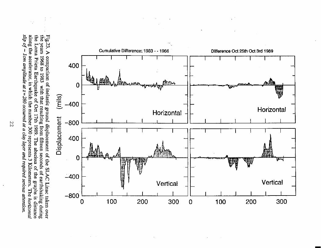
The cumulative motion of the tunnel floor for a seventeen year period is depicted in Fig. 23 on the left. The interpretations are as follows. The tunnel was constructed by the so called cut and fill method. Generally the parts of the tunnel that have sunk are on fill which is still sinking slightly today. The parts that are rising are in the cut regions which rebound due to the removal of overburden. By construction standards the overall motions are considered small and attest to the efficacy of the then soils engineering plan. In these regions the tunnel height is sensitive to water levels resulting from seasonal rainfall. The horizontal deformations result from unrelieved underground water pressure on the sides of the tunnel due to a long term failure of the drainage system. With two exceptions there is no evidence that the many ancient and geologically inactive faults that intersect the tunnel~produce any measurable discontinuities. The right side of Fig.23 is what happened in 15 seconds on Oct17 ‘89.

21

. . 8 z $ r 0 g ‘3 Q

3 E 3

i

I 1

I I

I I

I

.

14 ?sl

I I

I

I I

I I

.-

(qw) ~uawaaelds!a

Fig.23. A comparison of inelastic ground displacem

ent of the SLAC Linac taken over the years 1968 to 1983 with that resulting from

fifteen seconds of earthshaking during the Lom

a Prieta Earthquake of O

tt 17th 1989. The abscissa of the graphs is distance

along the accelerator, in which the number 300 represents 3 Kilom

eters. The horizontal slip of - Icm

amplitude at z =280 occurred at a clay layer and required serious attention.

22

4.5 Earthquake Prediction

In known seismicly active regions of the world the man on the street, better yet local civic authorities, want to know when the next one is coming. Unlike the case of predicting of the next eclipse, the models we have of the mechanism, while reasonable, are far from precise. As more of the crusts’ danger spots become ever more populated an ever increasing emphasis is being placed not only on preparedness, but on understanding the systematics. Since large events in a given area are, thankfully, rare, seismologists are turning to history to unearth the clues. And where history is badly, or not at all, recorded they are resorting to digging it out with pick and shovel by trenching across faults.

One example in which past systematics have been quite revealing is the case of Loma Prieta 1989, probably better studied than any event in recent history. It is no accident that two of the worlds foremost institutes of earthquake study sit on the northern and southern ends of the San Andreas fault. The U.S.Geological Survey in Menlo Park and the California Institute of Technology in Pasadena.

Examine for a moment a 20 year record of seismicity along the northern portion of the San Andreas shown in Fig. 24a. Figure b) depicts the vertical distribution of events

a1 01/01/69 - 07/31/69 _ 4 g

; ~~~~~~~~1~~~:

1 ’ ’ ’ ’ ’ ’ 0 20 40 60 an Ino 120 140 Iwl tno 200 z:n 740 ?hn 7Rl-i JO0 570 340 360

,1I~TANl’, (h&A)

bl Loma Prieta Earthquakes [10/12/69 - 10/19/69) A A’

40 sn no IO9 129 I40 Ihn IRO 700 ?Yl ?49 ?hO vn 300 320 340 360

ll1’~lAtll I (hl.4)

cl = aI*bI h 1’ __

z E

,y, k 71, 1’-TT-‘--T-‘,--, ,-‘T I 7’ 1 I

Fig. 24. Cross Section of Seismicity along the San Andreas Fault.

as a function of distance and depth in the days following Ott 17th. Notice in c) how neatly the event filled in the ‘seismic gap’. I will leave it up to the reader to decide where the next events will occur. You may now ask: “Why didn’t it rip all the way”?.That may have to do with the fact that the fault has a kink in its direction at a place called the Black Mountain discontinuity. The Loma Prieta event had no precursors. Scientists studying the rate of motion and past energy releases can derive recurrence times or probabilities to future ruptures. One such forecast (not prediction) is shown in Fig. 25. You may be sure these numbers are under constant scrutiny.

23

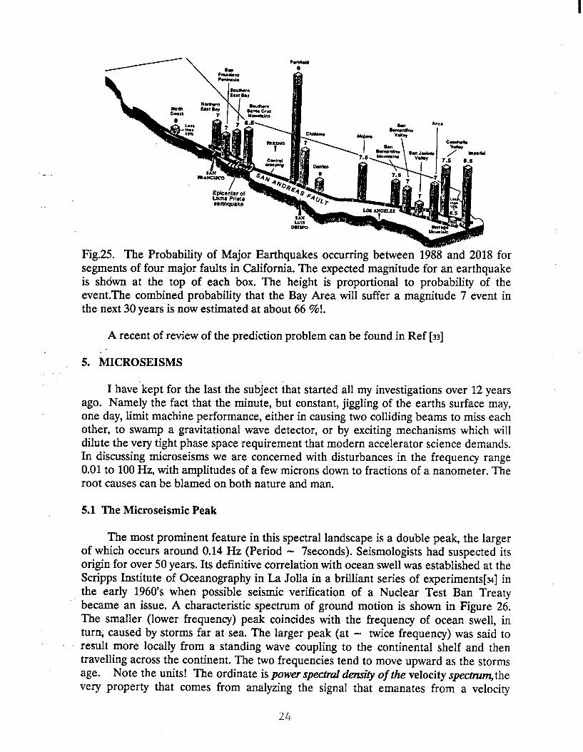
Fig.25. The Probability of Major Earthquakes occurring between 1988 and 2018 for segments of four major faults in California. The expected magnitude for an earthquake is shown at the top of each box. The height is proportional to probability of the event.The combined probability that the Bay Area will suffer a magnitude 7 event in the next 30 years is now estimated at about 66 %!.

A recent of review of the prediction problem can be found in Ref [33]

5. M~CROSEISMS

I have’kept for the last the subject that started all my investigations over 12 years ago. Namely the fact that the minute, but constant, jiggling of the earths surface may, one day, limit machine performance, either in causing two colliding beams to miss each other, to swamp a gravitational wave detector, or by exciting mechanisms which will dilute the very tight phase space requirement that modern accelerator science demands. In discussing microseisms we are concerned with disturbances in the frequency range 0.01 to 100 Hz, with amplitudes of a few microns down to fractions of a nanometer. The root causes can be blamed on both nature and man.

5.1 The Microseismic Peak

The most prominent feature in this spectral landscape is a double peak, the larger of which occurs around 0.14 Hz (Period - 7seconds). Seismologists had suspected its origin for over 50 years. Its definitive correlation with ocean swell was established at the Scripps Institute of Oceanography in La Jolla in a brilliant series of experiments[N] in the early 1960’s when possible seismic verification of a Nuclear Test Ban Treaty became an issue. A characteristic spectrum of ground motion is shown in Figure 26. The smaller (lower frequency) peak coincides with the frequency of ocean swell, in turn, caused by storms far at sea. The larger peak (at - twice frequency) was said to result more locally from a standing wave coupling to the continental shelf and then travelling across the continent. The two frequencies tend to move upward as the storms age. Note the units! The ordinate is power spectral density of the velocity specmmz,the very property that comes from analyzing the signal that emanates from a velocity

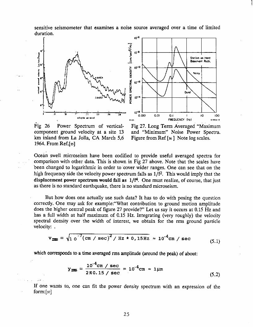
sensitive seismometer that examines a noise source averaged over a time of limited duration.

L I I I I I I u $1 ‘00 ,!’ 72 ?3 .x4 I!4 .IllLc+l I IILd \ Pig 26 Power Spectrum of vertical- component ground velocity at a site 13 km inland from La Jolla, CA March 5,6 1964. From Ref.[a]

10-6

m-lb

Stoiion on Hard Basement Rock.

‘” 0.001 0.01 0.1 I IO 100 6-E) FREOUENCY (Hz) Lt4IAlB

Fig 27. Long Term Averaged “Maximum and “Minimum” Noise Power Spectra. Figure from Ref [X ] Note log scales.

Ocean swell microseism have been codified to provide useful averaged spectra for comparison with other data. This is shown in Fig 27 above. Note that the scales have been changed to logarithmic in order to ‘cover wider ranges. One can see that on the high frequency side the velocity power spectrum falls as l/p. This would imply that the displacement power spectrum would fall as l/f4. One must realize, of course, that just as there is no standard earthquake, there is no standard microseism.

But how does one actually use such data? It has to do with posing the question correctly. One may ask for example:“What contribution to ground motion amplitude does the higher central peak of figure 27 provide ?” Let us say it occurs at 0.15 Hz and has a full width at half maximum of 0.15 Hz. Integrating (very roughly) the velocity spectral density over the width of interest, we obtain for the rms ground particle velocity: .

vm= o-'(cm/ se=)'/ Hz * 0,15Hz = 10-4cm / set /c 11

which corresponds to a time averaged rms amplitude (around the peak) of about:

y?.llS= 10-4c~ / set 2x0.15/ set

= 10-4cln = 1pm (5.2)

If one wants to, one can fit the power density spectrum with an expression of the form: [37]

25

P(f)= = t

v2 v v2+(f-9) 2l (5.3)

in which f. = 0.17 Hz, 2A/u = 7(rn/sec)2/Hz and Y = 0.03Hz and select the frequency band of interest over which to integrate.

Fig. 28 displays an overall compilation made available in 1986[ss]. Recently, particularly through the combined efforts with scientists in both the US and in the former Soviet Union, a great deal of high frequency (for geophysicists at least) data has become available for a number of sites. Particularly relevant is a recent series of articles that compares low noise high frequency spectra taken in both countries[39],[4o].

s- 3 c

; “7 az c= L:

!!i

2 6 K

= 2 8

I 90

.

-i

\- bQ \ ’

4 FV‘L SCALE 0 dS to SPS -. - - . _. _ -. - . .

%-

Ahi and Roehatds 1990

-50

-100

.-150

tW 0av.s 10 Dar% 1 Da” O.tDw -3)o -teal

w’ IO6 12 ,n4 d 90’ 10 1 01 001 owl

Fig.28. Ambient Noise Spectrum Compilation From Ref[38]. Fig.28. Ambient Noise Spectrum Compilation From Ref[38].

-1oq : : j : ::: -100~ : : j : ::: : : : : : : : :::: : :::: I :, : j I j: ..,. ..,. : : : :,;.:. : : .:::’ : : : : : : ::’ ! -120 - . . . . j . . j i...;. : j j ;;

: : : j . . : _ .: . . . . . . I: { ; : ::: : : :,;.: : : .:::’ : :

: : !

:

-120 - . . . . ..j.. . ..j i...;. : j j ;;

: : : ::’

: j . . : _ .: . ;.; I: { ;

:: : : i: ‘(i : :

: ‘: _: : ;,;i... I .._

: I ,111,ll I I

10-l 100 10' Frequency (Hz)

Fig.29. The lowest noise acceleration power spectrum observed at Station Garm (GAR) in the USSR in a vault blasted out of granitic rock in the side of a mountain in an area

of only small agricultural villages&at39 N,Long70 E.) The vertical component was taken at night and in the winter. DAS stands for data acquisition noise.From Ref. [39].

26

Notice the appearance of the 7 second microseism in the middle of the USSR. All this time I thought this signal was a property of the Pacific Ocean. At another station near Obninsk, near Moscow, located in a limestone vault 30 m below the surface, the 7sec signal is 20db larger in winter than in summer. Noise power levels increase dramatically in the ranges above 10 Hz when the sensors are at/near the surface (+ 10 db) and they are there sensitive to wind (+ 2db each lm/s increment of wind velocity above a threshold of 4-5 m/s.).

What does as all this have to do with accelerators or gravitational detectors? Fig 29 represents a noise figure which is about as low as nature will permit. It ( and its counterpart in other unpopulated areas ) is plenty good enough for todays and perhaps tomorrows accelerators, and about 200 db worse than what is needed for a gravitational detectors. From here on the noise situation gets steadily worse. Accelerators are not built in the wilderness (in spite of what some people say) and are therefore subject to the noise pollution caused by their very builders. Some machines are not even built on particularly hard (competent) ground. Of course one does not want to blast them out of granite; that is far too expensive. Regrettably some are being built in soft ground which, as we will see, is not the most technically best thing to do.

5.2 The Effects of Site Geology

I During the late 1960’s a certain gentleman decided to pack his Volkswagen bus with seismic gear and spent several years travelling through the German countryside in an attempt to ascertain if systematic ground noise measurements might reveal any systematic trends. They did! I have’chosen to reproduce below some of his illustrations (published in 1974 [41]) to make a point.

Fig.30. (on the 4W, -demo&rates graphically that’ in the spectral region we are interested in, that sensors placed in unconsolidated sediments appear to pick up much more seismic disturbance than those based on bedrock. I’m not sure about the units he uses,

t C km/HL] IOOC

IO” -

10-a -

10-J -

lo-’ -

Stationen auf Lockersedimentcn

there is either a power I I I I 8 I I 3 1 J 6 c

of two or a square root 7 f fiz] missing. But the effect is unmistakable.

He then made a scan through the Bavarian Jura and found the relationship shown in Fig 31. The deeper the Molasse overlying the harder Jura and Kristallin formations, the greater the sensitivity to microseismic disturbance.

27

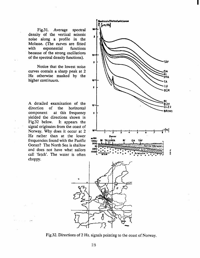
Fig.3 1. Average spectral density of the vertical seismic noise along a profile in the Molasse. (The curves are fitted with exponential functions because of the strong oscillations of the spectral density functions).

Notice that the lowest noise curves contain a sharp peak at 2 Hz otherwise masked by the higher continuum.

A detailed examination of the direction of the horizontal component at this frequency yielded the directions shown in Figf32 below. It appears the signal originates from the coast of Norway. Why does it occur at 2 Hz rather than at the lower frequencies found with the Pacific Ocean? The North Sea is shallow and does not have what sailors call ‘fetch’. The water is often ChOPPY-

lo

I

10

I

Iv

I

IO

1

lc

Bpehtrolr Dkht~bnhtlrron

t cmel

$I” CL22 BRw)

t I 1 I 1 2 J 4 s 6 7 +?I 8

DOMU muN

_. -- I

1000 SO0

0

1000 1 500

I-' . :

Fig.32. Directions of 2 Hz. signals pointing to the coast of Norway.

25

5.3 The Effects of Civilization

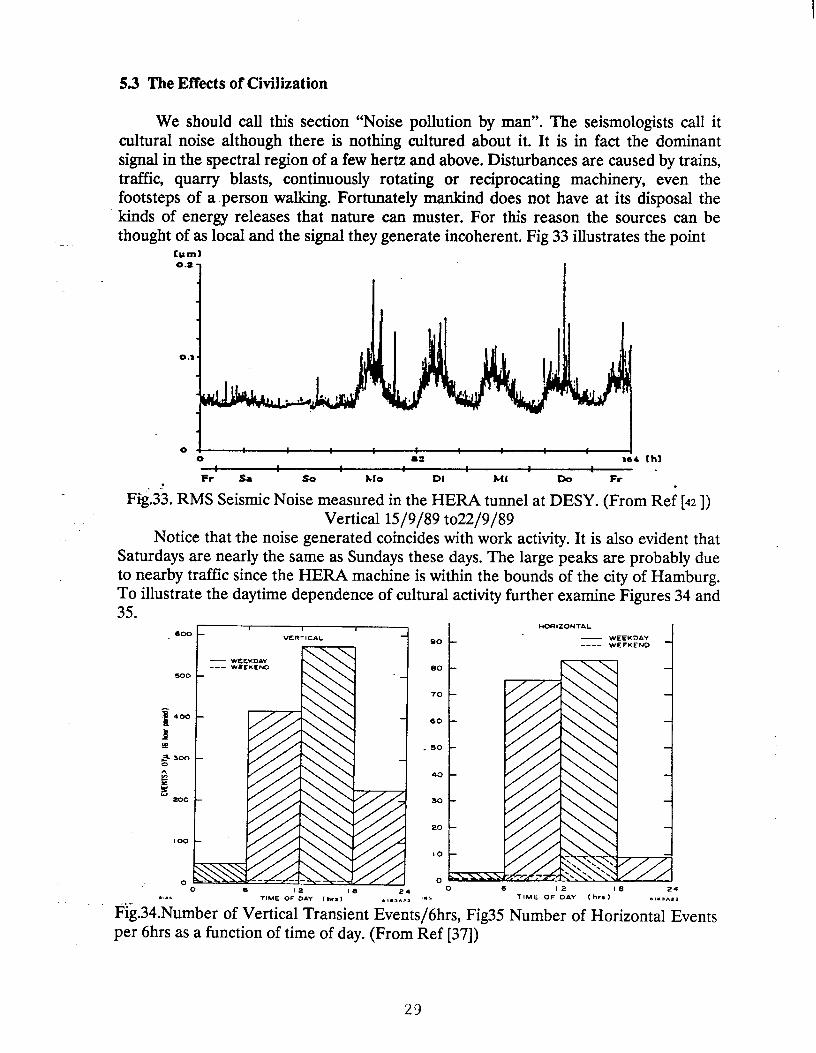
We should call this section “Noise pollution by man”. The seismologists call it cultural noise although there is nothing cultured about it. It is in fact the dominant signal in the spectral region of a few hertz and above. Disturbances are caused by trains, traffic, quarry blasts, continuously rotating or reciprocating machinery, even the footsteps of a person walking. Fortunately mankind does not have at its disposal the kinds of energy releases that nature can muster. For this reason the sources can be thought of as local and the signal they generate incoherent. Fig 33 illustrates the point

Cum1

0 02 166 thl

Fr Sa so MO Di Ml Do Fr . . .

F&33. RMS Seismic Noise measured in the HERA tunnel at DESY. (From Ref [42 1) Vertical 15/g/89 to22/9/89

Notice that the noise generated coincides with work activity. It is also evident that Saturdays are nearly the same as Sundays these days. The large peaks are probably due to nearby traffic since the HERA machine is within the bounds of the city of Hamburg. To illustrate the daytime dependence of cultural activity further examine Figures 34 and 35.

- WEEKDaY --- W2LKLe.o

r- e

* 300 0

1 f

r: zoo

100

0

t

HORIZONTAL 90 - WEEKDAY ---- WEEKEND

so

70

60

. 50

40

30

20

IO

0 0 6 15 24

.I. TIME OF’,‘, (hrs) csl.z.All

Fig.34.Number of Vertical Transient Events/6hrs, Fig35 Number of Horizontal Events per 6hrs as a function of time of day. (From Ref [37])

23

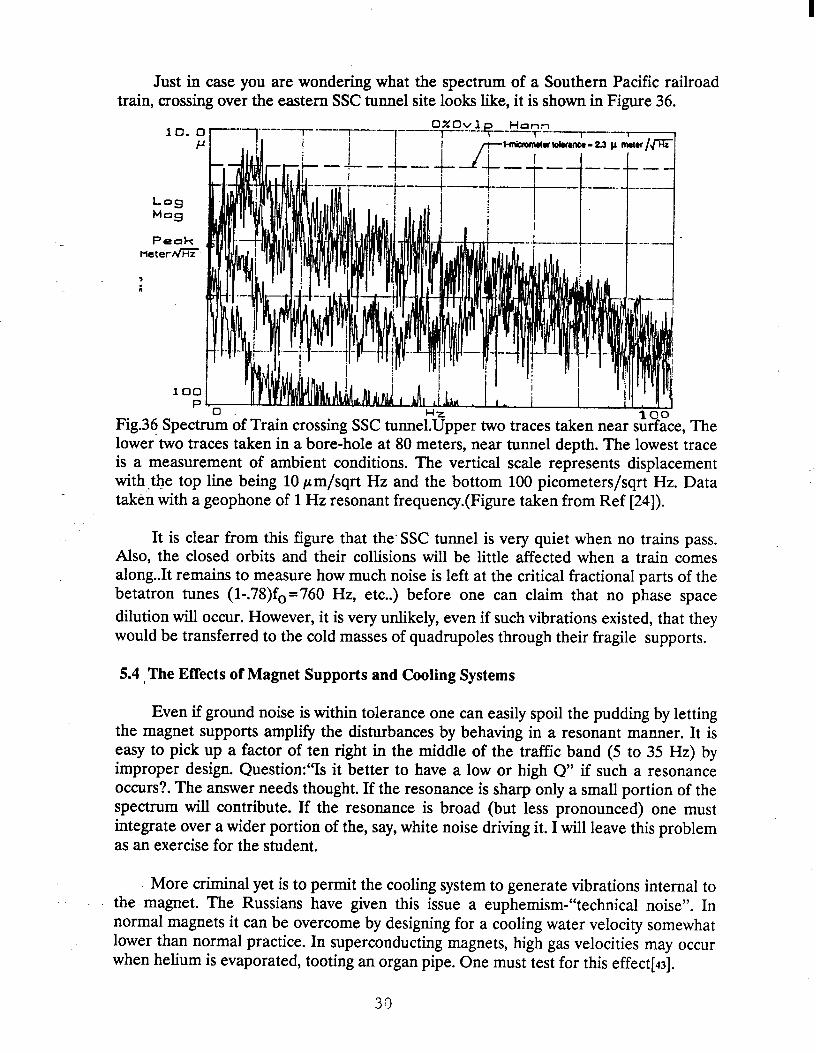
Just in case you are wondering what the spectrum of a Southern Pacific railroad train, crossing over the eastern SSC tunnel site looks like, it is shown in Figure 36.

of Train crossing SSC tunne per two traces taken near s lower’two traces taken in a bore-hole at 80 meters, near tunnel depth. The lowest trace is a measurement of ambient conditions. The vertical scale represents displacement with <the top line being 10 pm/sqrt Hz and the bottom 100 picometers/sqrt Hz. Data takkn with a geophone of 1 Hz resonant frequency.(Figure taken from Ref [24]).

It is clear from this figure that the. SSC tunnel is very quiet when no trains pass. Also, the closed orbits and their collisions will be little affected when a train comes along..It remains to measure how much noise is left at the critical fractional parts of the betatron tunes (l-.78)f, =760 Hz, etc..) before one can claim that no phase space dilution will occur. However, it is very unlikely, even if such vibrations existed, that they would be transferred to the cold masses of quadrupoles through their fragile supports.

5.4 , The Effects of Magnet Supports and Cooling Systems

Even if ground noise is within tolerance one can easily spoil the pudding by letting the magnet supports amplify the disturbances by behaving in a resonant manner. It is easy to pick up a factor of ten right in the middle of the traffic band (5 to 35 Hz) by improper design. Question:“Is it better to have a low or high Q” if such a resonance occurs?. The answer needs thought. If the resonance is sharp only a small portion of the spectrum will contribute. If the resonance is broad (but less pronounced) one must integrate over a wider portion of the, say, white noise driving it. I will leave this problem as an exercise for the student.

More criminal yet is to permit the cooling system to generate vibrations internal to the magnet. The Russians have given this issue a euphemism-“technical noise”. In normal magnets it can be overcome by designing for a cooling water velocity somewhat lower than normal practice. In superconducting magnets, high gas velocities may occur when helium is evaporated, tooting an organ pipe. One must test for this effect[a].

5.5 Countermeasures

.-

It seems to me that in todays high-tech world it is easy to forget that prevention is still the best medicine. Prevention can be practiced in a number of ways. The first, and most obvious, is’to design machines with parameters and lattices that are less sensitive to position errors. The second, perhaps even more obvious, is to prevent politicos from choosing sites that are severely beset by natural and man-made disturbances. Fortunately progress has been made on both of the above issues in the last several years. Third, it behoves management to remain ever vigilant so that good sites are not contaminated by bad housekeeping (such as by placing old fashioned reciprocating machinery near sensitive components or permiting variable temperatures, or worse yet, thermal gradients to polute the tunnel environment).

Next comes the application of a whole industry called vibration holation and dynamic alignment. The simplest application (passive) is that of a mass (the component) supported by a damped spring. Known to you as the damped harmonic ocsillator, its response function (transmissibility) is shown in Figure 38 below.

10

a01

\ l.21

\

\

\P

L

.I3

\

1 10

Fig.37. The Response of a simple harmonic oscillator to external driving frequencies.

Fig.38. The SHO Resonance Frequency versus “static” deflection in inches.

~

One can see that an isolation of one order of magnitude is achievable for driving frequencies say a factor of five above resonance for Q’s -C/Cc = 5. But there are two problems . Great care must be exersised that there are no serious sources driving the object near resonance, and if the disturbances we are trying to shield against are say centered in the region 5 to 30 Hz, then the resonance frequency should be around a few Hertz. This calls for a very soft spring constant as shown in Figure 38. A say 3 Hz resonate calls for a static deflection of one inch, a fact that is somewhat difficult to

31

swallow when the static alignment tolerances are in the microns. Clever methods have been devised to overcome this problem[s4], but which generally require a long term static reference system of high resolution.

Such considerations naturally lead to what is now called “active isolation”; very high-tech solutions applied to things like silent submarines and their weapons using “smart materials” as sensors and actuators[ss]. But we do not need to look only there. I am told that the suspension of some very modem cars contain active devices to take the bumps out of the ride. These are the solutions of the future since state of the art in this technology is still considered by many as “immature” and expensive at this time.

What options remain when we have played all these cards to the hilt? After the machine has been mechanically aligned as well as possible with the most modem means at hand, the accelerator world has always relied on that time honored fall back : Beam Feedback. Be it mechanical or electromagnetic, manual or automatic, fast or slow we have always relied on the application of beam derived intelligence to extricate us from the dilemma of not meeting alignment tolerances.

BUT, here too, there are limitations.

1. The ab initio alignment must be good enough to get the beam into the machine. _ : 2. It must be good enough that the solutions found by the correction system

algorithms converge. 3. It must be good enough so that the correction system does not introduce

anomalous dispersion or high order aberations. 4. The beam position monitors should not lie (too much)! 5. The rampant proliferation of feedback system may make a circular machine

inoperable due to the complexity of systems.

Still, I have confidence that we will find the answers. I think mostly through common sense.

6 CONCLUSION

In this hour we have talked about distances on scales from the astronomic to the subnanometer. Some relevant to the accelerator builder today, some others perhaps in the future. Although theories of the universe, inflation, phase transition or Higgs fields are made in heaven, accelerators will still be built on the ground. So, if some day, in some distant control room you are trying to make your machine run, please remember that you may have to correct for the phase of the moon, the weather, the level of the ground water, the traffic on nearby roads, or whether you closed the door to the tunnel and turned out the lights.

And the answer to that age old question: “ be: “You bet it did!”

Did the earth move for you?“[46] will

32

l Work supported by the U.S.Department of Energy under contract DE-AC03-76SF005l.5

REFERENCES

[I]. Diagram from the text “The Evolving Ear&,” by F.Sawkins et al. MacMillan Publishing Co.,1974

[2]. E.D.Courant and H.S.Snyder, Annals of Physics, Vol.3 No&Jan 1958 (Chapter 4a.)

[3]. J.Rossbach, PartAcc. Vol23,No.2 (1988), also DESY Report 89-023 Feb.1989

[s]. T.Raubenheimer SLAC Report 387, Thesis - Nov.1991 page 201 Table 16. and T.Himel, SLAC, - unpublished and private communication, Jan 1992.

[s]. From the Article “Shudders in the fabric of space-t ime” Nigel Henbest, New Scientist 1 Sept.1990

[6] For a quantatative mathematical treatment of the Gravitational Potential see “Physics of the Earth” F.D.Stacey, Second Edition 1977 Chapter 4.4 John Wiley and Sons.Inc. 414 p. QC806.s65 1977.

[7] (a)For a comprehesive treatment of all aspects and containing 2000 references see:“The tides of the planet .Earth” P.Melchior, 2nd Edition Pergammon Press Ltd. 1982 (b) Extensive theoretical material can be found in “Earth Tides” J.C.Harrison, Van Nostrand Reinhold Co. N.Y. 419p., QC809.E2E13 1985

[8] From the “Encyclopedia of Earth Sciences” Cambridge University Press. 1989?

[9] For a comprehensive review of this discipline see Proceedings of CERN Accelertor School - Applied Geodesy for Particle Accelerators April 1986 Editpr S.Tumer, published as CERN 87-01 Feb.1987

[IO] “Design and Operation of a Methane Absorption Stahl&d Laser Strainmeter” J.Levine and J.L.Hall Bull Seismological Sot Vol. p2595 1972

[ll] Albert Hoffmann, private communication Jan 15 1992

[12] M .D.Wood, Doctoral Thesis, Dept. of Geophysics, Stanford Univeristy, May 1%9

[13] “On charting Global Ocean Tides”, E.W.Schwiderski, Reviews of Geophysics and Space Physics, Vol.18 No.1 pages 243 1980. The coefficients of equations 1-4 in Table 1 are reproduced here in Appendix I

[14] Warburton and Goodkind 1978 in Ref. 7b

[ti] Studying the Earth by Very long Baseline Interferometry”, W.Carter and D. Robertson, Scientific American, November 1986

[la] “The Earth’s Rotation” J.M .Wahr Annual Reviews of Earth and Planetary Science 1988.16:231-49

[17] “Measuring Crustal Deformation in the American West” T.H.Jordan and J.B.M inster, Scientific American August !988.

[18] Most recent review “Measurement of Crustal Deformation using the Global Positioning System” B.H.Hager, R.W.King, and M .H. Murray, AnnRev. Earth planet.Sci.1991 19351-82 See also Ref.[9]. For work at SLAC see:“Application of GPS in a High Precision Engineering Survey Network”, SLAC- PUB-3620 R.Ruland, A.Leik ,lst Int.Symp.on Prec.Pos.with GPS, Rockwiile,MD 1985 pp483-494

‘. [19] “Space Age Geodesy - The NASA Crustal Dynamics Project, IEEE TransGeosci. Remote Sensing, Vol.GE-23,Number 4,Juiy 1985. R.J.Coates, H. V.Frey, G.D.Mead and JM.Bosworth

33

[ZO] See for example: Closing Adress: Challenge of the Future for Geodesy, J.Gervaise CERN 87-01 Feb 1987

[21] “Displacement of Surface Monuments:HorizontaI Motion” F.Wyatt, Journal of Geophysical Research, Vo1.87.NoB2 p979-989 February 10 1982.

[ZX] “The proposed ahgnment system for the Final Focus Test Beam,” R.E.RuIand, G.E.Fischer, Proc.of the Second International Workshop on Accelerator Alignment, DESY Hamburg Sept. 1990.

[23] One of the cornerstone articles in this field is: “On the Propagation of Tremors over the Surface of an Elastic Solid,” H.Lamb, Philosophical Transactions of the Royal Society,London, Ser. A, Vol203,ppl-42 1904

[a] Representative value of this material at tunnel depth from SSC Boring VE9.3 by Earth Technology Co. listed in SSC Report 1043 Table 6.1

[u]. “Seismic Waves: Radiation, Transmission and Attenuation”, J.E.White, McGraw HiII, N.Y. 1%5

[xi] “The Motion of the Ground in Earthquakes”, D.M.Boore, Scientific American, December 1977

[27] From an U.S.Govt. pamphlet: “The Loma Prieta Earthquake of Ott 17,1989” by Peter Ward and Robert Page, U.S.Govt.Printing Office 1989

[28] Figure kindly provided by Dan Ponti of the U.S.G.S Menlo Park (private communication) June 1990

[29] I “Earthquake Ground Motions” , T.H.Heatonand S.H.HartzeIl, Annual Reviews of Earth and Planetary Science 1988.16:121-45

[30] Paul Somerville-and Joanne Yoshimura of Woodward-Clyde Consultants, Pasadena, California

[31] A compilation of effects can be found in: “SLAC Site Geology, Ground Motion and Some Effects of the Ott 17,1989 Earthquake” G.E.Fischer SLAC-Report-358 Dee 1989

[32] “Precision Alignment Using a System of Large Rectangular Fresnel Lenses,” W.B.Hermannsfeldt et al., Applied Optics, Vo1.7.995 (1968)

[33 ] “Earthquake Prediction”, D.L.Turcotte, Ann.Rev.Earth Planet.Sci 1991.19263-81

[M] “Comparative Spectra of Microseisms and Swell”, RA.Haubrich,W.H.Munk and F.E.Snodgrass, Bull. of the Seismological Society of America Vo1.53, No.1 pp.27-37 January !%3

[x] Earth Noise, 5 to 500 Miicycies per Second” RA.Haubrich and G.S.MacKenzie, Journal of Geophysical Reasearch Vo1.70, No.6 !%5

[36] “Quantitative Seismology,” K.Aki and P.Richards, Freeman & Co. 1980 Vol I, Chapter 10

[37] “Ground Motion and Its Effects in Accelerator Design, G.E.Fischer, SLAC-PUB- 3392 Rev. 1985 and AIP Conference Series No.153 Summer School on High Energy Particle Accelerators, Batavia 1984.

[XX] Data compilation by R.Borcherdt, private communication, U.S.G.S. Menlo Park, CA

[39] Variations in Broadband Seismic Noise at IRIS/IDA Stations in the USSR with Implications for Event Detection, H.K.Given, Bulletin of the SeismiIogicaI Society of America, Vol.80 No.6,pp2072-2088, Dee 1990

[40] Analysis of High Frequency Seismic Noise in the Western United States and Eastern Kazakstan”, H.Gurrola, et al. BuII.Seis.Soc. Am. Vo1.8O,No.4 pp951-970 Aug.1990.

34

[41] “Systematische Untersuchung der kurxperiodischen seismischen Boderumruhe in der Bundesrepublik Deutschland”, M.Steinwachs, Geologosches Jahrbuch, Reihe E, (Geophysik) E3 Hannover 1974

[42 ]“HERA Errors and Related Experiences during Commissioning ” J.Rossbach DESY HER4 91-21 Dee 1991.

[43] For example: “Measurement of the Motion of Superconducting Quadrupole Magnets at Liquid Helium Temperatures”, W.Decking,K.Fiottmann, DESY HERA 90-09 and in European Particle Accelerator Conference,(EPAC),Rome 1987

[#I See for example those adopted by industry as exemplified by Optical tables by the Newport Corporation 18235 Mt.Baldy Circle Fountain Valley, CA 92728 USA Catalog 1990 part A.

[SS] These concepts, long known to the space and weapons community were discussed recently at the ‘Workshop on Vibrational Control and Dynamic Alignment at the SSC” held in Dallas, Texas, Feb.ll-14 1992 Joe Weaver (Chairman)

[46] I am indebted to Bill Kirk (SLAC) for pointing out that this phrase derives from Hemingway’s “For Whom the Bell Tolls”. I also thank him for reading the manuscript and valuable comments.

35