Earthquake Ground Motion Selection · Earthquake Ground Motion Selection. i ... earthquake ground...
60
May 2012 Steven L. Kramer Pedro Arduino Samuel S. Sideras WA-RD 791.1 Office of Research & Library Services WSDOT Research Report Earthquake Ground Motion Selection
Transcript of Earthquake Ground Motion Selection · Earthquake Ground Motion Selection. i ... earthquake ground...
May 2012Steven L. Kramer Pedro ArduinoSamuel S. Sideras
WA-RD 791.1
Office of Research & Library Services
WSDOT Research Report
Earthquake Ground Motion Selection


i
Research Report Research Project T4118, Task 69
EARTHQUAKE GROUND MOTION SELECTION
by
Steven L. Kramer Pedro Arduino
Samuel S. Sideras
Department of Civil and Environmental Engineering University of Washington
Washington State Transportation Center (TRAC) University of Washington, Box 354802
1107 NE 45th Street, Suite 535 Seattle, Washington 98105-4631
Washington State Department of Transportation
Technical Monitor Tony Allen
State Geotechnical Engineer
Prepared for
The State of Washington Department of Transportation
Paula J. Hammond, Secretary
May 2012

ii
1. REPORT NO. 2. GOVERNMENT ACCESSION NO. 3. RECIPIENTS CATALOG NO
WA-RD 791.1
4. TITLE AND SUBTITLE 5. REPORT DATE
Earthquake Ground Motion Selection May 2012
6. PERFORMING ORGANIZATION CODE
7. AUTHOR(S) 8. PERFORMING ORGANIZATION REPORT NO.
Steven L. Kramer, Pedro Arduino, Samuel S. Sideras
9. PERFORMING ORGANIZATION NAME AND ADDRESS 10. WORK UNIT NO.
Washington State Transportation Center (TRAC) University of Washington, Box 354802 1107 NE 45th Street, Suite 535 Seattle, WA 98105-4631
11. CONTRACT OR GRANT NO.
T4118-69
12. CO-SPONSORING AGENCY NAME AND ADDRESS 13. TYPE OF REPORT AND PERIOD COVERED
Washington State Department of Transportation Research Office, PO Box 47372 Olympia, WA 98504-7372 Research Manager: Kim Willoughby 360.705.7978
Final Report 14. SPONSORING AGENCY CODE
15. SUPPLEMENTARY NOTES
This study was conducted in cooperation with the U.S. Department of Transportation, Federal Highway Administration.
16. ABSTRACT
Nonlinear analyses of soils, structures, and soil-structure systems offer the potential for more accurate characterization of geotechnical and structural response under strong earthquake shaking. The increasing use of advanced performance-based design and evaluation procedures will require consideration of long-return-period motions for all structures, especially in western Washington where high seismicity is a concern and long-return-period motions are likely to be strong enough to induce nonlinear, inelastic response in soil deposits and structures. Nonlinear analyses require the specification of acceleration time histories as input; this requires the analyst to identify input motions that are consistent with the ground motion hazards at the site of interest. A considerable level of research effort has been directed toward the development of procedures for selection and scaling of earthquake ground motions for the purpose of using them in nonlinear structural analysis. This research has shown that structural response of buildings can be quite sensitive to the selection and scaling of ground motions used in nonlinear analyses. While the sensitivity of bridge structures to input motion characteristics has not been studied as explicitly as that of building structures, the response of bridges is also expected to be significantly influenced by input motion characteristics. As a result, engineers have identified the need for software tools that will automate, to at least a large degree, the process of identifying suites of ground motions that are most appropriate for use in nonlinear response analyses. Along with this report, a piece of software, SigmaSpectraW, was created for WSDOT to do just that.
17. KEY WORDS 18. DISTRIBUTION STATEMENT
Earthquake, ground motion selection, SigmaSpectraW
19. SECURITY CLASSIF. (of this report) 20. SECURITY CLASSIF. (of this page) 21. NO. OF PAGES 22. PRICE
None None

iii
DISCLAIMER
The contents of this report reflect the views of the authors, who are responsible for the facts and
the accuracy of the data presented herein. The contents do not necessarily reflect the official
views or policies of the Washington State Department of Transportation or the Federal Highway
Administration. This report does not constitute a standard, specification, or regulation.
iv
Table of Contents
Chapter 1 Introduction 1 Background 1 Organization of Report 3 Chapter 2 Available Ground Motion Processing Tools 4 PEER Ground Motion Database 4 SigmaSpectra 6 Baker Codes 7 Conclusions 7 Chapter 3 Target Spectra 9 Uniform Hazard Spectrum 9 AASHTO Design Spectrum 11 Conditional Mean Spectrum 12 Risk-Targeted Ground Motions 15 Site Effects 16 Discussion 17 Chapter 4 Washington State Ground Motion Database 18 State-Wide Locations 18 Representative Locations 21 Ground Motion Selection 23 Database Organization 25 Earthquake Characteristics 26 Chapter 5 Ground Motion Selection and Scaling Software Package – SigmaSpectraW 28 Input Data 28 Output 33 Exporting Data 35 Comments on Use of Program 36 Chapter 6 Summary 38 References 40 Appendix A – Metadata for Spectrum-Consistent Motions 42 Appendix B – Metadata for Long Duration Motions 46 Appendix C – Metadata for Near-Fault Motions 51

1
Chapter 1
Introduction
The practice of seismic design has been developing rapidly over the past 20-30 years.
Observations of response and damage in recent earthquakes, focused research supporting the
development of performance-based design concepts, and developments in computer software and
hardware have led to the increased use of numerical analysis in the seismic evaluation of existing
structures and the seismic design of new structures. While structures have been designed using
response spectra and modal superposition for many years, the use of nonlinear analysis has been
increasing.
Background
Nonlinear analyses of soils, structures, and soil-structure systems offer the potential for
more accurate characterization of geotechnical and structural response under strong earthquake
shaking. Bridge and building codes require the evaluation of seismic response for ground
shaking levels with relatively long return periods, e.g., on the order of 975 to 2,475 years. Also,
the increasing use of advanced performance-based design and evaluation procedures will require
consideration of long-return-period motions for all structures. In areas of low seismicity, long-
return-period motions may not be particularly strong and response spectrum or equivalent linear
analyses may be appropriate. In seismically active areas such as western Washington, however,
long-return-period motions are likely to be strong enough to induce nonlinear, inelastic response
in soil deposits and structures.
Linear and equivalent linear analyses can be accomplished with the use of response
spectra alone, i.e., without explicit consideration of individual ground motion time histories. Site
effects can be estimated using ground motion prediction equations (GMPEs) or amplification
factors. Even equivalent linear site response analyses can be performed without time histories
when random vibration theory (RVT) procedures are used. Nonlinear analyses, however, require
the specification of acceleration time histories as input; this requires the analyst to identify input
motions that are consistent with the ground motion hazards at the site of interest. A considerable
2
level of research effort has been directed, particularly within the past 10 years or so, toward the
development of procedures for selection and scaling of earthquake ground motions for the
purpose of using them in nonlinear structural analysis. This research has shown that structural
response of buildings can be quite sensitive to the selection and scaling of ground motions used
in nonlinear analyses. While the sensitivity of bridge structures to input motion characteristics
has not been studied as explicitly as that of building structures, the response of bridges is also
expected to be significantly influenced by input motion characteristics.
Bridges, like other structures, tend to respond most strongly to loading at or near their
natural frequencies (or periods). One simple approach to ground motion selection and scaling is
to scale a suite of input motions to a target spectral acceleration at the fundamental period of the
structure of interest. Such an approach will result in a suite of motions with no dispersion at the
fundamental period of the structure (i.e., all of the scaled spectra would pass identically through
the same point), but would result in significant dispersion at higher and lower periods. Higher
periods are important, however, because the effective period of a structure tends to lengthen as
damage occurs under strong shaking. Lower periods are also important because higher modes
will respond to higher frequency (lower period) components of the motions. As a result,
nonlinear analyses using motions scaled to match only a single point on a target spectrum will
produce computed responses with high levels of uncertainty. The practical impact of that result
is that more analyses (i.e., analyses using larger suites of input motions) will be required to
predict the mean (or median) response with a given level of confidence. To obtain a good
estimate of response with a relatively small suite of input motions, the motions should be
selected with consideration of spectral shape – motions whose response spectra are consistent
with the shape of the design spectrum over a range of periods both greater and lower than the
fundamental period will provide improved predictions of structural response.
As a result of increased ground motion instrumentation and the natural occurrence of
earthquakes over time, engineers now have access to thousands of recorded earthquake ground
motions. These motions are from earthquakes that have occurred around the world, and
represent a wide range of earthquake magnitudes, source-to-site distances, types of faulting, and
site conditions. The process of selecting a small suite of motions that optimally match some
desired target spectrum from these thousands of motions (and millions of combinations thereof)
is extremely time-consuming when attempted manually. As a result, engineers have identified

3
the need for software tools that will automate, to at least a large degree, the process of
identifying suites of ground motions that are most appropriate for use in nonlinear response
analyses.
Organization of Report
This report presents the results of a project undertaken at the University of Washington to
provide the Washington State Department of Transportation (WSDOT) with software tools that
aid in the selection and scaling of earthquake ground motions for geotechnical and structural
response analysis. The following chapters describe the process by which appropriate software
and data were collected and modified to provide WSDOT with a useful system.
Chapter 2 describes the results of a survey of available ground motion processing
software and an evaluation of their relative suitability for use by WSDOT. Chapter 3 provides
background on the types of target spectra used to define ground motion hazards – spectra used in
current codes and spectra likely to be used in future codes. Chapter 4 describes the software
recommended for use by WSDOT in ground motion selection and scaling, which is a modified
version of an existing software program, and Chapter 5 describes a ground motion database that
was assembled for use with the software described in Chapter 4. Chapter 6 presents a brief
summary of the work completed for the project.

4
Chapter 2
Available Ground Motion Processing Tools
Several software tools for selecting and scaling earthquake ground motions are currently
available. The tools all have different capabilities and operate with different databases and
interfaces. All are relatively new so there is very little in the way of a track record with any of
them. The following sections briefly review the three most significant tools that are currently
available.
PEER Ground Motion Database
The Pacific Earthquake Engineering Research (PEER) Center has been collecting,
processing, and archiving ground motion data for the past 15 years or so. In order to facilitate
the original Next Generation Attenuation (NGA) research effort, PEER began collecting
recorded motions from shallow crustal earthquake in active tectonic regimes and had Dr. Walter
Silva of Pacific Engineering & Analysis, Inc. process all of the motions in a consistent manner.
The motions were then posted online as the 2005 PEER NGA Database. The NGA database
could be accessed and searched on the basis of source (magnitude, distance, style of faulting,
etc.) and site (e.g., site class, Vs30) conditions. After some time, PEER contracted GeoMatrix to
lead a team of researchers and practitioners in development of the Design Ground Motion
Library (DGML), an anticipated stand-alone program that would allow the selection and scaling
of ground motions relative to a target response spectrum. After an extended period of
development, the decision was made to modify this effort from a stand-alone program to a web-
based utility; a beta version of the PEER Ground Motion Database system was recently brought
online at:
http://peer.berkeley.edu/peer_ground_motion_database

5
This link currently provides two options – searching and selecting motions without scaling, and
searching and scaling ground motions.
The second option is most applicable to the problem at hand. The website allows a user
to define a target spectrum; code- and GMPE-based options can be selected or a user-defined
target spectrum can be entered. After entering the target spectrum, the user initiates a search of
the PEER database for motions that are consistent with the target spectrum. Ranges of
parameters including magnitude, style of faulting, duration, source-to-site distance, Vs30, and
scaling factor can all be specified. In addition, the inclusion or exclusion of motions with near-
fault pulses can be specified. Finally, the user can input a weighting function that allows the
matching algorithm to consider matching at some periods to be more important than others when
identifying motions. The program returns a list of 30 motions in ranked order of spectral match
quality. Clicking on each motion produces time history plots of all three (fault-normal, fault-
parallel, and vertical) components of acceleration (with one-click ability to plot velocities and
displacements) and highlights the selected motion on a plot of all 30 response spectra. The
selected motions are easily downloaded for subsequent use.
Advantages
The PEER system is well-designed and implemented, and the online utility is easy to use
and runs relatively quickly – it is also freely available to all users. It has access to the PEER
database, which is the most extensive and well-developed ground motion database in existence.
The PEER database is maintained by PEER, so its updating requires no effort on the part of the
user.
Disadvantages
The PEER system is constrained to use of the PEER database, which contains only
motions from shallow crustal earthquake in active tectonic regimes. This restriction, which may
be removed at some undetermined point in the future, presents difficulties for WSDOT in that
the seismic hazards facing structures in many parts of Washington state are significantly
influenced by potential Cascadia Subduction Zone (CSZ) earthquakes. Subduction zone events
emanate from greater depths than crustal earthquakes, can be of considerably greater magnitude

6
than crustal earthquakes, and can produce ground motions with significantly longer durations
than crustal earthquakes.
SigmaSpectra
SigmaSpectra is a stand-alone computer program that selects suites of ground motions
whose mean matches a target spectrum and scales the suite to match a target standard deviation.
In this manner, SigmaSpectra can produce ground motions that tightly match a target spectrum
(by entering a target standard deviation of zero) or match it with some desired level of
dispersion. SigmaSpectra first selects suites of motions that match the target spectrum and then
scales them to match the target standard deviation while maintaining the mean at the level of the
target spectrum.
SigmaSpectra does not come with a pre-defined ground motion database (other than a
small database used for the example problem in the program tutorial). It does allow the user,
however, to develop a database that motions can be drawn from to develop ground motion suites.
While development of a ground motion database can be time-consuming, the user has unlimited
flexibility in selecting motions from different sources.
Advantages
SigmaSpectra is a public domain program for which the source code is available, thus
allowing the possibility of modification to add useful features. The manner in which the ground
motion data is made available to the program allows great flexibility in customizing the database
for different tectonic environments – this advantage is particularly significant in a state with such
different levels of sources of seismicity. The code is a stand-alone program that resides on the
user’s computer and is therefore not susceptible to website or internet availability problem,
which can occur with a web-based utility like the PEER Ground Motion Database. Finally,
SigmaSpectra has a graphical user interface that allows convenient examination and comparison
of ground motions.
Disadvantages
In contrast to the PEER system, a SigmaSpectra user must build, maintain, and update a
ground motion database, which can be time-consuming. The algorithm by which SigmaSpectra

7
searches for optimal suites of ground motions can be inefficient, leading to long runtimes for
large databases and/or large requested suite sizes.
Baker Codes
A third software tool has been developed by Prof. Jack Baker and colleagues at Stanford
University. This tool consists of a suite of Matlab programs that can also select suites of ground
motions whose mean matches a target spectrum and scales the suite to match a target standard
deviation. The Baker codes use a different approach to that of SigmaSpectra and can complete
the selection and scaling process more quickly for a given ground motion database.
The Baker codes come with no ground motion data, although they make use of ground
motion meta-data such as that contained in the NGA flatfile assembled by PEER. A user can
develop an extended flatfile with ground motion data from other events. The Baker codes have
no graphical user interface – data can be plotted in Matlab or written to text files for processing
by another graphics program.
Advantages
Like SigmaSpectra, the Baker code is publicly available in source code form, and is
resident on the user’s computer. The user can build a database that includes ground motions
from different sources. The Baker codes are efficient, and can identify an optimum suite of
ground motions considerably faster than SigmaSpectra.
Disadvantages
Again, as with SigmaSpectra, the user has responsibility for the ground motion database.
The Baker code is written in Matlab, a powerful programming language that is not familiar (or
available) to many practicing engineers. Finally, the Baker code does not have a graphical user
interface.
Conclusions
The PEER Ground Motion Database system has many attractive capabilities and may
eventually represent the best long-term approach for ground motion selection and scaling.
However, the limitations of the database itself, i.e., the lack of subduction zone motions, for

8
ground motion hazards in Washington state render it ineffective for short-term use by WSDOT.
The length of time that will be required for the database to be expanded to the point at which this
system can be used effectively to represent the ground motion hazards that exist in Washington
state is not known at this time; given the time required to develop the first version of this system
and PEER’s current focus on development of GMPEs for the central and eastern United States, it
is likely that it will be several years before the PEER utility reaches that state.
The Baker code package is computationally efficient and highly capable, but has no user-
friendly interface and would likely require significant effort to master for ground motion
selection. Furthermore, the Matlab language in which it is written is not widely available. A
graphical user interface could be wrapped around a compiled version of the Baker codes, but
development of such an interface would be time-consuming and acquisition of a Matlab compiler
expensive.
The SigmaSpectra software tool is capable of performing the type of ground motion
selection and scaling that is needed, but does so slowly for large ground motion databases. With
an optimized database of moderate size, however, SigmaSpectra can operate with acceptable
speed. The current version of SigmaSpectra has good graphics capabilities, but not all of the
capabilities that WSDOT would like to see; as a result, some modification of SigmaSpectra
would be required.
Based on the preceding review, SigmaSpectra was selected as the platform for ground
motion selection and scaling. A number of modifications to the original SigmaSpectra code
were made to allow presentation of additional data and processing of ground motion data. In
order to allow the modified program to operate efficiently, a ground motion database, termed
here the Washington State Ground Motion Database (WSGMDB) was developed. By
eliminating ground motions that are not appropriate (or are redundant with respect to other
motions) for sites in Washington state, the number of potential ground motion suite combinations
can be reduced dramatically. The WSGMDB is a database containing ground motion from
multiple sources which have spectral amplitudes and shapes that are generally consistent with
AASHTO design spectra at various locations across Washington state.

9
Chapter 3
Target Spectra
The level of ground shaking used for structural design is generally defined in terms of
one or more design response spectra. The design spectra are usually determined from the results
of a probabilistic seismic hazard analysis (PSHA) and represent ground motions with a particular
mean rate of exceedance, or return period. The use of design spectra with specified return
periods allows differences in seismicity to be accounted for in seismic design; for the same
return period, the design spectra in areas of high seismicity have higher ordinates than those in
areas of low seismicity.
Several different types of spectra can be computed and used for design. If a design is to
be based on a goal of elastic structural behavior, the design can be based directly on the design
spectrum using modal superposition. Modern seismic design, however, allows some level of
inelastic response and increasingly requires the use of nonlinear structural analyses; these, in
turn, require ground motion time histories as input. The design spectra then become targets for
which ground motions with consistent shapes are sought. The selection and scaling of recorded
ground motions to match or exceed some target spectrum is an important part of seismic design.
Defining, and understanding, the target spectrum is an important part of that process.
Uniform Hazard Spectrum
PSHAs are commonly performed with spectral acceleration, Sa(T), as a ground motion
intensity measure. Performing a suite of PHSAs for spectral acceleration at different structural
periods will produce a series of spectra acceleration hazard curves (Figure 3.1a). By selecting a
particular mean annual rate of exceedance, a set of Sa(T) values can be obtained and plotted as a
function of period (Figure 3.1b). The hazard curves for different periods, T, are performed
independently of each other, i.e., without consideration of hazard levels at other periods. The
ordinates of the resulting response spectrum all have the same return period, and the spectrum is

10
known as a uniform hazard spectrum, or UHS. Uniform hazard spectra can be computed for
different return periods.
Figure 3.1. Construction of uniform hazard spectrum: (a) Spectral acceleration hazard curves for different
structural periods (rotated 90o from usual presentation), and (b) Spectral accelerations at design return period, TR, plotted vs. structural period.
Deaggregation of uniform hazard spectra reveals important characteristics that should be
recognized when using them for design purposes. Consider the 975-yr return period UHS for
Seattle shown in Figure 3.2. Deaggregation of the spectral accelerations at different periods
produce the mean magnitude, distance, and ε values shown in Table 3.1. The parameter, e,
describes the number of (logarithmic) standard deviations an intensity measure is above the
(logarithmic) mean. Note that the values are different – the Sa(0.1) hazard, for example, is
associated with lower magnitude, shorter distance events while the Sa(3.0) hazard is coming from
higher magnitude, greater distance events. This characteristic of UHS behavior is well
recognized – the UHS includes weighted contributions from many different earthquake scenarios
(i.e., combinations of magnitude and distance). The result of this characteristic is that, in many
cases, no single earthquake event is capable of producing a motion with a response spectrum that
matches the entire UHS. Some motions may be consistent with a UHS at lower periods but are
weaker at long periods, while others may be consistent at long periods and weaker at short
periods. In areas dominated by a single seismic source, the UHS may be consistent with the
spectra produced by individual events.

11
Period, T 0.0 6.81 43.0 1.11 0.1 6.78 40.5 1.09 0.2 6.94 39.4 1.04 0.3 6.98 43.8 1.05 0.5 7.15 51.8 1.10 1.0 7.49 62.5 1.04 2.0 7.75 75.0 1.00 3.0 7.81 76.0 0.93 4.0 7.97 74.0 0.71 5.0 7.81 65.8 0.74
Figure 3.2. 975-yr uniform hazard spectrum for Seattle, WA.
Table 3.1. Mean magnitudes, distances, and epsilon values for 975-yr spectral accelerations at different
structural periods.
Uniform hazard spectra are often used as targets for ground motion selection. Most
codes specify that a suite of ground motions used for design match (individually or as an
ensemble average) or exceed the UHS over some significant period range. The significant
period range is typically keyed to the fundamental period of the structure and extends to longer
periods (to account for damage-related period lengthening during shaking) and lower periods (to
account for higher-mode response). The significant period range (frequently from 0.2To to
1.5To) may be wide enough, however, that no individual ground motion can reasonably be
expected to have a spectrum that matches or exceeds the UHS over that entire range. If that is
the case, the motions are generally scaled upward until they meet the code criteria – the motions
are then likely to be excessively energetic for the desired hazard level. The scaled motions then
represent an actual hazard level that is higher (e.g., corresponds to a longer return period) than
intended. A recent study of ground motion selection and modification procedures for buildings
(Haselton, 2009) showed that motions selected on the basis of UHS compatibility produced
median maximum interstory drift ratios that were biased (high) by a factor of about 1.3.
AASHTO Design Spectra
While site-specific probabilistic seismic hazard analyses may be warranted for major
bridge projects or in areas where new understanding of seismic hazards has recently developed,
most bridges are designed on the basis of 1,000-yr return period ground motions. The AASHTO
LRFD Specifications (2007, 2009) provide guidance for development of design spectra.

12
The AASHTO spectra are smoothed versions of uniform hazard spectra with standard
shapes keyed to spectral accelerations at periods of 0.0, 0.2, and 1.0 sec. The U.S. Geological
Survey (USGS) has developed a computer program and database
(http://earthquake.usgs.gov/hazards/designmaps/aashtocd.php). The program provides data for
developing 1,000-yr spectra for site class B/C (Vs = 760 m/sec), and uses AASHTO
amplification factors to account for the effects of local soil conditions. Figure 3.3 illustrates the
type of spectrum produced by the AASHTO procedure.
Figure 3.3 AASHTO design spectrum produced by USGS AASHTO
Earthquake Ground Motion Parameters computer program.
Conditional Mean Spectrum
The UHS implicitly assumes that the ground motions from each scenario exceed the
median level by a nearly constant amount at all periods – actual earthquake spectra, however,
have irregular shapes that cause the amount by which they exceed (or fall below) the median to
fluctuate significantly with period. While the ε values for a particular spectrum at two closely-
spaced periods are likely to be closely correlated to each other, their correlation decreases when
the periods are farther apart. Baker and Cornell (2006a) showed that the correlation coefficient
for ε values at two periods, Tmin and Tmax, could be approximated as

13
+−−= <
min
maxmin)189.0(maxmin ln
189.0ln163.0359.0
2cos1),(
min TTTITT T
πρ
where Tmin and Tmax are the lower and higher of the two periods, respectively, and )189.0( min<TI is
an indicator variable equal to 1 if Tmin< 0.189 and 0 otherwise. Figure 3.4 illustrates the
correlation between ε (hence, also Sa(T)) values at a period of interest, T* = 1.0, and other
periods; the correlation coefficient is 1.0 at the selected period but drops off at periods above and
below the selected period. The expected value of ε at periods other than the period of interest is
given by
*)(*),(*)()|( TTTTT ερµ εε =
Figure 3.4. Correlation between Sa(T) values at T = 1.0 sec and other periods.
So the expected value of the (logarithmic) response spectrum conditional upon *)(Tε is given by
)(),,( ln*)()|(ln*)()|ln(ln TTRMaaaa STTSTSTS σµµµ εε+=
The corresponding spectrum is referred to as the conditional mean spectrum (CMS). The
median spectral accelerations are therefore given by
[ ]TTTTTRMTSaa SSa (*)(*),(),,(exp)( lnln σερµ +=
The distribution of spectral acceleration at all periods given the value of Sa(T*) can be obtained
from *)()|ln(ln TSTS aaµ and
2ln*)()|ln(ln *),(1)( TTTSaTSTS aa
ρσσ −=

14
Figure 3.5 illustrates the relationship between the CMS and the constant ε (i.e., ε(T) = ε(T*))
scenario spectrum. Note that the CMS falls below the constant ε spectrum at periods other than
T*, which reflects the actual behavior of individual ground motions.
Figure 3.5. Relationship between spectrum with constant ε spectrum and corresponding CMS.
The CMS can be used as a target for ground motion selection, typically with T* set to the
fundamental period of the structure of interest. To cover the range of ground motions that could
be expected at a particular site, however, multiple CMS with different T* values (Figure 3.6)
may be required. Ground motions can also be selected to match the distribution of spectral
acceleration in order to estimate the distribution of computed response.
Figure 3.6. Use of multiple CMS to cover broad range of periods.
The CMS provides a more realistic spectrum than the UHS for a given Sa(T*) in that it
has a shape consistent with the shapes of individual ground motions. This shape is based on

15
deaggregation data (M, R, and ε) and ground motion prediction equations, so the shape changes
with amplitude in a manner consistent with that observed in actual earthquakes. Haselton (2009)
found that motions scaled to fit a CMS produced median maximum interstory drift ratios that
were biased (high) by a factor of only 1.01, a value much lower than that (1.3) obtained for
motions scaled to fit a UHS. On the other hand, CMS data is less readily available than UHS at
this point in time and, given that the CMS changes with amplitude and period of interest,
multiple sets of ground motions may be required for design purposes.
While current codes do not specifically address the use of the CMS for design, it may be
appropriate for individual projects and may very well become part of future codes. From the
standpoint of record selection and scaling, the use of CMS-based target spectra presents no
particular difficulties – in fact, better fits are likely to be obtained with a CMS target spectrum
than a UHS target spectrum.
Risk-Targeted Ground Motions
In recent years, the concept of risk-targeted ground motions has developed to the point at
which it is being used in some current building codes. Risk-targeted ground motions seek to
define ground motions that will result in a defined mean annual rate of exceedance of some
specified risk level. For buildings, the risk is that of collapse and risk-targeted motions have
been developed for a 1% probability of collapse in a 50-yr period, i.e., a collapse return period of
4,975 yrs. The calculations are performed by combining a probabilistic collapse model (one that
provides fragility curves describing the probability of collapse conditional upon ground motion
intensity) with a ground motion intensity hazard curve. The resulting collapse hazard curve
accounts for uncertainty in the ground motion and uncertainty in the hazard given the ground
motion.
In effect, risk-targeted ground motions account for the entire hazard curve since the risk
is obtained by integrating over all levels of ground motion intensity. Thus, hazard curves with
different shapes will produce different risk-targeted ground motions even if the ground motion
hazard curves are similar at the return period of interest. Such an approach, which is analogous
to the performance-based approach to liquefaction hazard analysis developed by Kramer and
Mayfield (2007), allows more uniformity of performance than is obtained by current procedures.
Comparing risk-targeted motions with MCE motions from previous codes (e.g., ASCE-07), the

16
risk-targeted motions are significantly (more than 15%) weaker along the Pacific coast of
Washington.
Site Effects
Target spectra used for design should account for the effect of local soil conditions on
ground surface motions. Site effects can be determined in two primary ways – through the use of
amplification factors (which are increasingly incorporated into ground motion prediction
equations, or GMPEs) or through site-specific response analyses.
Amplification factors, whether computed separately or contained within GMPEs, are
obtained from regression upon empirical data from multiple sites and earthquakes. As a result,
an amplification factor is consistent with the average characteristics of the soil profiles in the
database from which it was developed. This characteristic can be important in deciding whether
or not a site-specific analysis should be performed (it may not be necessary for sites that have
average characteristics, e.g., a shear wave velocity profile that increases smoothly with depth),
and in deconvolution operations (motions consistent with average velocity profiles should be
deconvolved through an average velocity profile rather than a site-specific profile).
When site conditions differ significantly from average conditions, site effects are better
accounted for by performing site-specific response analyses. Equivalent linear or nonlinear
analyses that take individual shear wave velocity profiles and material characteristics into
consideration can be used. When relatively large shear strains (greater than about 1%) are
encountered, nonlinear analyses can produce more reasonable results than equivalent linear
analyses. When soils capable of generating significant excess porewater pressure are present,
nonlinear effective stress analyses should be performed.
Site effects can also influence the type of target spectrum to use in ground motion
selection. Because uniform hazard spectra have been criticized as being excessively strong,
engineers tend to consider their use as being conservative with the expectation that stronger input
motions will lead to stronger seismic response. For a soft soil profile (or strong shaking level),
however, motions fit to a uniform hazard spectrum can “overdrive” a soil profile in a site
response analysis leading to reduced ground surface motions at some frequencies. If such
ground surface motions are used as inputs to a structural analysis, the structure may be subjected
to loading that is not consistent with the expected return period.

17
Discussion
The use of target spectra for selection of earthquake ground motions allows engineers to
identify ground motions with amplitudes and frequency contents that are generally consistent
with some intended ground motion hazard level. It should be recognized, however, that a
response spectrum provides an incomplete representation of an earthquake ground motion – put
differently, many different ground motions could have (nearly) the same response spectrum and
could induce very different levels of response in structures. For a suite of motions, these
differences can lead to dispersion (scatter) in the computed response.
The principal ground motion characteristic that is not well reflected in the response
spectrum is duration. Duration is known to affect many aspects of seismic response, particularly
for soils. While duration is rarely evaluated explicitly in seismic hazard analyses, it varies with
both magnitude and distance and can therefore be at least roughly inferred from the results of
deaggregation analyses. With respect to ground motion selection, the likelihood of obtaining
motions with appropriate durations is increased by restricting the pool of candidate motions to
those with magnitudes and distances that are consistent with those that contribute most strongly
to the ground motion hazard at the return period of interest.

18
Chapter 4
Washington State Ground Motion Database
In order to streamline the ground motion selection and scaling process for transportation
structures in Washington, a Washington State Ground Motion Database (WSGMDB) was
assembled. The purpose of the WSGMDB was to provide WSDOT with a relatively small
database of ground motions with amplitude, frequency content, and duration characteristics
similar to those of design ground motions in Washington State. The availability of this
Washington-specific database would allow existing software tools for ground motion selection
and scaling to be used efficiently in Washington State with only limited modifications.
The ground motions were selected with consideration of AASHTO bridge design code
seismic standards, which are based on design response spectra with nominal 975-yr return
periods (i.e., with 5% probability of exceedance in a 50-yr period). The selection process also
considered consistency with source characteristics such as magnitude and distance. The process
by which the WSGMDB motions were identified is described in the following sections.
State-Wide Locations
In order to provide appropriate geographic coverage of the entire state, and to recognize
the different levels of seismicity in different parts of the state, a set of 34 cities (Figure 4.1) were
identified for consideration of design response spectra. Probabilistic seismic hazard analyses
were performed for each of the cities using the USGS National Seismic Hazard Mapping
project’s Interactive Deaggregations website (https://geohazards.usgs.gov/deaggint/2008/) in
order to determine the nature of the earthquake events that contribute most strongly to ground
motion hazard at the locations of the various cities. The specific locations, and mean magnitudes
and distances for each of the cities are listed in Table 4.1.

19
Figure 4.1. Locations at which AASHTO design spectra were computed.
Table 4.1. Locations, mean magnitudes, and mean distances at 975-yr hazard level for 34 locations.
City Location Mean Deaggregated Values Group Latitude Longitude M R (km) Bellingham 48.80 122.53 6.65 54.20 C Bremerton 47.48 122.77 7.05 45.20 A Burlington 48.50 122.33 6.73 52.40 C Colville 48.88 118.47 6.04 46.40 D Ephrata 47.32 119.52 6.14 45.90 D Everett/Paine 47.92 122.28 6.89 33.60 B Fairchild 47.62 117.65 5.95 34.40 D Fort Lewis 47.08 122.58 6.91 52.70 B Goldendale 45.82 120.82 6.62 76.6 D Hanford 46.57 119.60 6.19 43.30 D Hoquiam 46.97 123.97 8.30 30.80 A Kelso/Longview 46.14 122.93 7.78 66.8 C Long Beach 46.35 124.06 8.6 27.8 A McChord AFB 47.15 122.48 6.85 52.40 B Moses Lake 47.20 119.32 6.08 40.20 D Oak Harbor 48.25 122.68 6.97 42.10 B Olympia 46.97 122.90 7.21 54.50 B Omak 48.42 119.53 6.03 32.30 D Pasco 46.27 119.12 6.12 37.10 D Port Angeles 48.12 123.50 7.35 35.00 B Pullman 46.75 117.12 5.96 38.30 D Quillayute 47.95 124.55 8.55 27.00 A Renton 47.50 122.22 6.77 36.70 A Seattle 47.45 122.30 6.81 38.90 A

20
Shelton 47.25 123.15 7.40 49.60 B Spokane 47.63 117.53 5.94 33.30 D Stampede Pas 47.28 121.33 6.45 47.10 C Tacoma 47.27 122.58 6.89 51.90 B Toledo 46.48 122.80 7.38 62.10 C Vancouver 45.63 122.69 7.37 59.7 C Walla Walla 46.10 118.28 5.96 29.10 D Wenatchee 47.40 120.20 6.41 64.90 D Whidbey Island 48.35 122.65 6.87 41.20 B Yakima 46.57 120.53 6.40 58.50 D
AASHTO design response spectra were then generated for each of the 34 cities using the
AASHTO Seismic Design Parameters program
(http://earthquake.usgs.gov/hazards/designmaps/aashtocd.php) developed by the U.S. Geological
Survey. The Seismic Design Parameters program provides spectral response ordinates at periods
ranging from 0 – 4 sec. The design response spectra for all 34 locations are shown in Figure
4.2(a); the spectral ordinates can be seen to cover a wide range due to the different levels of
seismicity at the widely spaced locations. Figure 4.2(b) shows the same design spectra
normalized with respect to PGA– in this form, the different spectral shapes also reflect the
different seismicities of the different locations. In particular, the different magnitudes that
contribute to seismicity cause significant differences in long-period spectral amplitudes.
Figure 4.2. (a) Design spectra for 34 locations, and (b) normalized design spectra for 37 locations.

21
Representative Locations
The design spectra shown in Figure 4.2(a) lend themselves to division into several
categories. The spectral acceleration amplitudes, while covering a wide range, tend to fall into a
relatively small number of groups, the most obvious being those spectra from locations east of
the Cascade mountain range, i.e., from central and eastern Washington, which have maximum
spectral acceleration values below 0.40 g. Four groups were defined as having maximum
spectral acceleration values in the ranges shown in Table 4.2. Within each of these amplitude-
based groups, spectral shapes were examined to identify locations with similar amplitudes but
different spectral shapes. Figure 4.3 shows the normalized spectra broken down by amplitude
group; all but Group C include spectra with significantly different shapes, particularly, Groups A
and D. To cover the ranges of both amplitudes and spectral shapes within the 34 original
locations, a subset of 10 sites with significantly different design spectra that encompassed the
range of design spectra of the larger group of 34 locations was developed. The 10 spectra are
shown, along with the other 24 spectra, in Figure 4.4. The spectra for the representative
locations can be seen to span the range of amplitudes and spectral shapes that exist within the
larger group of original locations.
Table 4.2. Amplitude groups for selection of design spectra.
Group Maximum Sa Range
A (Sa)max> 0.95 g
B 0.75 g < (Sa)max< 0.95 g
C 0.60 g < (Sa)max< 0.75 g
D (Sa)max< 0.40 g

22
Figure 4.3. Design response spectra for: (a) Group A, (b) Group B, (c) Group C, and (d) Group D.
Figure 4.4. Response spectra for all locations with representative locations highlighted.

23
Ground Motion Selection
The selection of earthquake ground motion records for seismic evaluation and design
requires consideration of target spectrum matching by scaled motions, but also of ground motion
characteristics not necessarily reflected in response spectra. As a result, three groups of ground
motions were identified for inclusion within the WSGMDB: (1) motions that are consistent with
the previously described target spectra, (2) long-duration ground motions that would be
representative of interplate subduction zone earthquakes, and (3) near-fault ground motions that
include directivity pulses representative of those expected at sites near surface faults such as the
Seattle fault.
Spectrum-Consistent Motions
A process was developed to identify recorded ground motions that were consistent with
the design spectra for the 10 representative locations. A number of ground motion databases are
available worldwide, including those listed in Table 4.3. All of the databases in Table 5.3 were
queried to obtain records for consideration in assembly of the WSGMDB. The different
databases had different search capabilities ranging from those that searched for motions based on
compatibility with a target spectrum (e.g., PEER NGA database) to those that could search only
on the basis of magnitude, depth, and location (e.g., K-Net database). It should be noted that the
motions in the K-Net database have not been processed.
Table 4.3. Sources of strong ground motion records.
Database URL
PEER NGA http://peer.berkeley.edu/peer_ground_motion_database/spectras/new
COSMOS http://db.cosmos-eq.org/scripts/search.plx
CESMD http://www.strongmotioncenter.org/cgi-bin/ncesmd/search1.pl
K-Net http://www.k-net.bosai.go.jp/
The databases listed in Table 4.3 were queried to obtain candidate records for inclusion in
the WSGMD. Where possible, target spectra consisting of the 10 representative location design
spectra were entered and motions that matched those spectra were identified. For databases

24
without target spectrum-matching capabilities, ranges of source parameters (e.g., magnitude,
distance, style of faulting) were used to identify motions most likely to be consistent with design
spectra. These searches produced a preliminary set of 280 ground motions that were further
examined for consistency with the 10 representative location design spectra.
Due to the similarity of some of the design spectra, a number of duplicate records (i.e.,
records that provided good fits to more than one design spectrum) were obtained. Nevertheless,
each representative location design spectrum was well-matched by at least 20 different ground
motion records. This led to a final set of 226 motions from which individual records could be
selected and scaled to produce good approximations to AASHTO design spectra from within
Washington state. The individual motions, and their pertinent characteristics, are summarized in
Appendix A.
Long-Duration Motions
Ground motion hazards for structures located near the Pacific coast and for longer-period
structures located farther inland, e.g., along the I-5 corridor, are influenced by interplate
earthquakes on the Cascadia Subduction Zone. The mean magnitudes for coastal locations such
as Hoquiam, Quillayute, and Long Beach, for example, are all considerably greater than 8.0,
which indicate strong contributions from large CSZ interplate events. Large-magnitude
earthquakes are known to produce long-duration ground motions. Therefore, a suite of long-
duration ground motions was developed by searching through several ground motion databases
for records from large-magnitude earthquakes. Because large-magnitude events are rare, not
many have been well-recorded by modern strong motion instruments; in some cases, the
recorded motion database can be supplemented by synthetic ground motions. The recent 2011
Tohoku earthquake, however, was very well recorded by the K-Net and Kik-Net seismographic
networks in Japan.
A suite of 241 recorded and 180 simulated long-duration motions was assembled. Many
available long-duration ground motions were recorded at distant locations, hence the amplitudes
are low enough that excessively large scaling factors would be required to produce reasonable
spectral matches; such motions were not included in the final suite of long-duration motions.
138 of the recorded long-duration motions are from the 2011 Tohoku earthquake in Japan – these
motions have been baseline-corrected and lightly (0.02 – 50 Hz bandpass) filtered but not

25
instrument-corrected or otherwise processed; the motions should be reviewed, processed as
necessary, and approved by a qualified engineering seismologist prior to use. The suite of
simulated motions were developed by Dr. Walter Silva of Pacific Engineering and Analysis for a
previous WSDOT study (Kramer et al., 1998). The individual long-duration motions and their
pertinent characteristics are summarized in Appendix B.
Near-Fault Motions
Ground motions at sites near earthquakes frequently exhibit near-fault characteristics
including directivity pulses and fling step. The constructive interference of waves emanating
from a rupture front moving toward a site can cause a long-period pulse of motion referred to as
a directivity pulse, which is stronger in the fault-normal (FN) direction than the fault-parallel
(FP) direction. Fault rupture can also cause a permanent displacement in the slip direction in the
near-fault region; this displacement, which is in the FP direction for strike-slip and FN direction
for dip-slip events, is referred to as a fling step displacement.
A suite of 182 near-fault motions, all of which have been identified as containing
directivity pulses (Baker, 2007) was assembled; the individual motions and their pertinent
characteristics are summarized in Appendix C.
Database Organization
The process described in the preceding section produced a total of 829 motions with
potential applicability to the design of transportation structures in Washington state. These
motions comprise the WSGMDB, and are organized as indicated in Figure 4.5.

26
Figure 4.5 Organization of Washington State Ground Motion Database (WSGMDB).
The manner in which the database is organized was developed to simplify the use of
SigmaSpectraW. Because the program will use the motions in all subfolders within a user-
specified master folder, the database can be optimized for individual sites. If the user wants
SigmaSpectraW to consider all 829 motions in the WSGMDB, he/she would simply select the
All Motions folder in the path requested on the input screen (Figure 5.1). If the user wanted
SigmaSpectraW to consider only the motions within one of the regional databases, he/she would
simply select the folder for the path. If the user wanted SigmaSpectraW to consider, for
example, all non-K-Net long-duration motions in addition to the regional motions, he/she could
copy the Other recorded long-duration motions folder into the regional folder and select the
regional folder for the path. In this way, the user is given complete flexibility in selection of the
motions to be considered. It is recommended that the user keep a record of the database used in
his/her project files.
Earthquake Characteristics
The ground motions in the WSGMDB were produced by 38 different earthquakes with
different magnitudes, source-to-site distances, styles of faulting, etc. Table 4.4 presents source
data for these earthquakes; these data can be used to assist in the selection of ground motions.

27
Table 4.4 Characteristics of earthquakes producing ground motions in the WSGMDB.
Earthquake Year Mw Strike (deg)
Dip (deg)
Style of faulting
Hyp. Lat.
(deg)
Hyp. Long. (deg)
Hyp. Depth (km)
Surface Rupture
Big Bear-01 1992 6.46 55 85 Strike-slip 34.2100 -116.8300 13.0 N
Cape Mendocino 1992 7.01 350 14 Reverse 40.3338 -124.2294 9.6 N
Chi-Chi, Taiwan 1999 7.62 5 30 Reverse-Oblique 23.8603 120.7995 6.76 Y
Chi-Chi, Taiwan-02 1999 5.90 35 50 Reverse 23.9400 121.0100 8.0 Chi-Chi, Taiwan-03 1999 6.20 0 10 Reverse 23.8100 120.8500 8.0 Chi-Chi, Taiwan-04 1999 6.20 330 89 Strike-slip 23.6000 120.8200 18.0 Chi-Chi, Taiwan-05 1999 6.20 165 70 Reverse 23.8100 121.0800 10.0 Chi-Chi, Taiwan-06 1999 6.30 5 30 Reverse 23.8700 121.0100 16.0 Coalinga-01 1983 6.36 137 30 Reverse 36.2330 -120.3100 4.6 N
Coalinga-05 1983 5.77 355 38 Reverse 36.2410 -120.4090 7.4 N
Coalinga-07 1983 5.21 348 38 Reverse 36.2290 -120.3980 8.4 N
Coyote Lake 1979 5.74 336 80 Strike-slip 37.0845 -121.5054 9.6 Y
Denali, Alaska 2002 7.90 296 71 Strike-slip 63.5375 -147.4440 4.86 Y
Erzican, Turkey 1992 6.69 122 63 Strike-slip 39.7050 39.5870 9.0 N
Hector Mine 1999 7.13 331 77 Strike-slip 34.5740 -116.2910 5.0 Y
Imperial Valley-06 1979 6.53 323 80 Strike-slip 32.6435 -115.3088 9.96 Y
Irpinia, Italy-01 1980 6.90 313 60 Normal 40.8059 15.3372 9.5 Y
Irpinia, Italy-02 1980 6.20 124 70 Normal 40.8464 15.3316 7.0 Kobe, Japan 1995 6.90 230 85 Strike-slip 34.5948 135.0121 17.9 Y
Kocaeli, Turkey 1999 7.51 272 88 Strike-slip 40.7270 29.9900 15.0 Y
Landers 1992 7.28 336 90 Strike-slip 34.2000 -116.4300 7.0 Y
Loma Prieta 1989 6.93 128 70 Reverse-Oblique 37.0407 -121.8829 17.48 N
Mammoth Lakes-06 1980 5.94 22 50 Strike-slip 37.5060 -118.8260 14.0 N
Morgan Hill 1984 6.19 148 90 Strike-slip 37.3060 -121.6950 8.5 Y
N. Palm Springs 1986 6.06 287 46 Reverse-Oblique 34.0000 -116.6117 11.0 N
Norcia, Italy 1979 5.90 341 64 Normal 42.7300 12.9600 6.0 N
Northridge-01 1994 6.69 122 40 Reverse 34.2057 -118.5539 17.5 N
Northwest China-03 1997 6.10 21 45 Normal 39.5557 76.9477 20.0 San Fernando 1971 6.61 287 50 Reverse 34.4400 -118.4100 13.0 Y
San Salvador 1986 5.80 32 85 Strike-slip 13.6330 -89.2000 10.9 N
Sierra Madre 1991 5.61 242 50 Reverse 34.2591 -118.0010 12.0 N
Sitka, Alaska 1972 7.68 347 90 Strike-slip 56.7700 -135.7840 29.0 N
Superstition Hills-02 1987 6.54 127 90 Strike-slip 33.0222 -115.8314 9.0 Y
Tabas, Iran 1978 7.35 330 25 Reverse 33.2150 57.3230 5.75 Y
Taiwan SMART1(40) 1986 6.32 43 57 Reverse 24.0817 121.5915 15.8 N
Westmorland 1981 5.90 64 90 Strike-slip 33.1000 -115.6200 2.3 N
Whittier Narrows-01 1987 5.99 280 30 Reverse-Oblique 34.0493 -118.0810 14.6 N
Yountville 2000 5.00 150 90 Strike-slip 38.3788 -122.4127 10.12 N

28
Chapter 5
Ground Motion Selection and Scaling Software Package – SigmaSpectraW
As discussed in Chapter 2, the SigmaSpectra software program (Kottke and Rathje,
2010)was selected as the base platform on which to build a ground motion selection and scaling
system that would be appropriate for WSDOT. A number of modifications to the original
SigmaSpectra program were made to provide information and utilities requested by WSDOT
personnel – the modified program is called SigmaSpectraW. This chapter describes the basic
operation of the modified program, drawing heavily on the user manual for the original program.
Input Data
SigmaSpectraW, like the original SigmaSpectra program, opens with a screen (Figure
5.1) that contains four dialog group boxes: target response spectrum, period interpolation, library
of motions, and calculations. The data required to run the program is entered by the user in these
sections.
Figure 5.1 Initial input screen for SigmaSpectraW

29
Target Response Spectrum
The target response spectrum section allows the user to enter the spectrum against which
the selected motions will be compared. The oscillator damping ratio can be specified by the
user, but is commonly taken as 5%. The target spectrum data is entered in terms of spectral
acceleration values at each of a user-determined set of oscillator periods. The program also
requests the (natural) logarithmic standard deviation, aSlnσ , at each period – this value will be
zero when the goal is to match a particular uniform hazard or conditional mean spectrum. To
account for ground motion variability in motions representing some earthquake scenario, the
value of aSlnσ , obtained from an appropriate ground motion prediction equation (GMPE), can be
provided so that the program will search for suites of motions that match both a target spectrum
and target dispersion. The Plot button allows a plot of the target spectrum to be seen in a
separate window. For convenience, the target spectrum data can be imported from a spreadsheet
by a simple copy-and-paste operation. It should be noted that the natural variability of actual
spectra, along with the limited number of motions in the ground motion database will prevent the
standard deviation of the optimum suite of motions from matching the target standard deviation
at all periods.
Period Interpolation
If desired, the entered target response spectrum data can be interpolated between to
produce a higher-resolution target spectrum against which candidate ground motion spectra can
be compared. To interpolate the target spectrum data, the check box within the Target Response
Spectrum section must be checked, and the period spacing (linear or logarithmic), minimum and
maximum periods, and number of interpolated points (between the minimum and maximum
periods) entered. A minimum of 25 points per log cycle of period is recommended for
logarithmic interpolation. The interpolation is accomplished using a cubic spline procedure
which cannot model sharp corners in target spectra, so this procedure may not be appropriate for
some (e.g., code-based) target spectra – it is strongly recommended that the user plot and
confirm the validity of the target spectrum prior to beginning the analysis. In some cases, the
target spectrum may be better constructed outside of SigmaSpectraW (e.g., using a spreadsheet)
at a large number of periods, and then pasted into SigmaSpectraW without interpolation.

30
Significant Period Range
The original version of SigmaSpectra considered the entire range of periods when
identifying optimum suites of motions. SigmaSpectraW allows the user to identify a range of
significant periods within which the suites are optimized. The lower and upper bound periods
are specified by the user; portions of the spectra outside this significant period range are not
considered when evaluating the suite’s fit to the target spectrum.
Library of Motions
After the target spectrum has been properly specified, SigmaSpectraW requires the user
to set the parameters of the search for optimum suites of motions. The values of these
parameters will affect the quality of the identified motions and the speed with which they will be
identified. The individual items in the Library of Motions section are described below.
Select Path
The ground motion database from which candidate motions are to be selected is defined
by its path. The user should specify a “master” folder within which the candidate motions exist –
one folder containing all of the candidate motions may be specified, or the motions may be
organized in subfolders within the master folder.
The speed with which the optimum suites of motions will be identified depends strongly
on the number of motions in the ground motion database. If speed is important, the selected
database should not contain motions that are unlikely to provide a good individual match to the
target spectrum. To assist in this process, SigmaSpectraW is accompanied by a ground motion
database that is organized into four regional databases which have been preliminarily screened to
eliminate motions that do not reasonably fit AASHTO design spectra within those regions.
Figure 5.2 shows the boundaries of the four regions; motions can be added to or removed from
these regional databases, or they can be subdivided into smaller regions as the user desires. The
regions were identified on the basis of spectral amplitudes and shapes. Region 1 represents the
coastal region where seismicity is strongly influenced by subduction zone events. Region 2 is
approximately the Puget Sound Basin, where intraplate, interplate, and crustal events all
influence seismicity. Region 3 is the region south of the Puget Sound Basin where subduction

31
zone events are significant but more distant than in the coastal region. Finally, Region 4 is
primarily central and eastern Washington where seismicity is relatively low.
Figure 5.2 Regions used to develop regional ground motion databases.
SigmaSpectraW gives the user complete flexibility in selecting the ground motion
database from which the suite of motions will be selected. The user can move individual motion
files, or folders containing multiple motions, in or out of the master folder. If a site is on the
border between two of the regions shown in Figure 4.2, for example, folders containing the
motions from the two regions can be pasted into a new master folder for the purposes of that
analysis.
Number of Motions in Suite
SigmaSpectraW is intended to search for a suite of motions whose logarithmic mean is as
close as possible to a defined target spectrum. The size of the suite is determined by the user,
and generally will be controlled by code requirements – suites of seven motions are commonly
specified by code documents. Larger suites require consideration of more combinations of
motions and, therefore, have longer runtimes.

32
Seed Combination Size
To speed up the optimum suite identification process, SigmaSpectraW uses a procedure
that avoids checking all possible combinations of motions within the ground motion database.
The seed combination size value will affect the rate and accuracy of the identification process; a
seed value of 2 has been shown to result in identification of the same motions identified
considering all combinations, but to do so in a much shorter period of time.
Suites to Save
The program can save as many suites of motions as the user requests. The various
combinations of motions comprising candidate suites are ranked by quality of fit; the requested
number of suites will be saved in order of quality of fit.
Combine Components
Individual motions can be considered in the ground motion selection process or pairs of
orthogonal horizontal motions can be considered. If the latter is selected, the motions are
selected on the basis of their geometric mean spectra – the geometric mean spectral acceleration
of a ground motion record with x- and y-components would be given by yaxa SS ,, ⋅ .
Flag Motions …
The Flag Motions button will load all ground motions in the specified ground motion
database and allow plots of acceleration, velocity, and displacement time histories to be
displayed. The name of each file along with a Flag utility is also displayed. Double-clicking the
shaded circle in the Flag column will allow the user to specify whether the selected motion is
required to be part of each considered suite (Required), barred from being within the considered
suites (Disable), or considered without prejudice (Unmarked). The Marked option can be used to
define a group of motions from which some user-specified number (specified in the Marked
textbox to the right of the Flag Motions button) will be included in each considered suite.
Calculation
The Calculation section contains a window in which the process of the ground motion
selection is displayed and the Compute button that initiates that process.
33
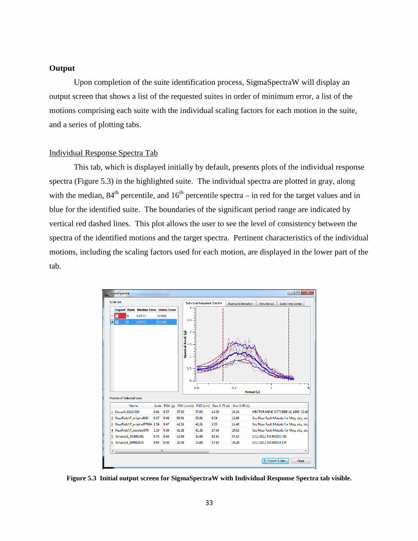
Output
Upon completion of the suite identification process, SigmaSpectraW will display an
output screen that shows a list of the requested suites in order of minimum error, a list of the
motions comprising each suite with the individual scaling factors for each motion in the suite,
and a series of plotting tabs.
Individual Response Spectra Tab
This tab, which is displayed initially by default, presents plots of the individual response
spectra (Figure 5.3) in the highlighted suite. The individual spectra are plotted in gray, along
with the median, 84th percentile, and 16th percentile spectra – in red for the target values and in
blue for the identified suite. The boundaries of the significant period range are indicated by
vertical red dashed lines. This plot allows the user to see the level of consistency between the
spectra of the identified motions and the target spectra. Pertinent characteristics of the individual
motions, including the scaling factors used for each motion, are displayed in the lower part of the
tab.
Figure 5.3 Initial output screen for SigmaSpectraW with Individual Response Spectra tab visible.

34
Standard Deviation Tab
The standard deviation tab simply shows the standard deviation of the identified spectra
plotted as a function of period.
Time Series Tab
The characteristics of individual motions are easily viewed using the Time Series tab.
Clicking once on an individual motion in the lower part of the tab will produce plots of
acceleration, velocity, and displacement as functions of time. These plots (Figure 5.4) are useful
for visualizing ground motion characteristics and confirming baseline correction.
Figure 5.4 Output screen for SigmaSpectraW with Time Series tab visible.
Suite Time Series Tab
It is often useful to compare ground motion time histories with each other. The Suite
Time Histories tab (Figure 5.5) allows up to seven motions to be plotted simultaneously. Note
that the motions are individually scaled so the acceleration and time scales may be different.

35
Figure 5.5Outputscreen for SigmaSpectraW with Suite Time Series tab visible.
Exporting Data
The scaled earthquake motions can be exported for use by other programs. Suites can be
selected for export using the check boxes in the first column of the Suite List on the main output
window. Suites that have been marked for export are exported by clicking the Export Suites
button in the lower right portion of the output window. The suite can be exported in a variety of
formats. The most general use is the comma-separated values (CSV) format as it also includes
the response spectra of each ground motion in the suite. Information for each suite is exported to
a different file name, the prefix of which can be specified. If the “Include Time Histories”
checkbox is checked, each scaled ground motion time history is saved to an independent file; the
name of which is established using the prefix, suite number, and motion number (e.g. suite1-
m1.eq). If the “CSV” radio button is checked, the format style specified in the “General
earthquake file format” group box is used. This group box allows the specification of the
number of header lines at the beginning of the file, the number of columns of acceleration data,
the field width (total number of characters including decimal points and +/- signs) of each
acceleration value, and the number of digits to the right of the decimal point for each
acceleration value. If the “NGA” or “Shake200” radio buttons are checked this format option is
not enabled since for these cases the formats are fixed and hardwired in the code.

36
Comments on Use of Program
SigmaSpectraW should be viewed as a tool to be used in the process of selecting ground
motions for use in seismic analysis and design. It is not, and should not be viewed as, a
complete, turnkey solution to the ground motion selection and modification process.
SigmaSpectraW will assist an engineer or seismologist in selecting suites of spectrum-consistent
motions from a database – it is the obligation of the user, however, to ensure that the database
contains appropriate motions and that the suites of motions identified by SigmaSpectraW are
appropriate for the specific site of interest. This means that the user should be familiar with
basic concepts of seismology and earthquake engineering, and should have some experience in
dealing with earthquake motions.
SigmaSpectraW should be used in an iterative manner. Using ground motion databases
such as those within the WSGMDB without any user interaction can result in suites of ground
motions populated by motions that fit the target spectrum well, but do not necessarily represent
ground motion hazards well. The databases cover wide areas within which ground motion
hazards may vary significantly – fine-tuning the database to the specific site of interest may be
required to obtain an optimal suite of ground motions. A series of potential problems and with
suggested solutions are described in Table 5.1.
Table 5.1 Potential problems and solutions with ground motion selection process.
Problem Effect Solution Suite contains too many motions from same earthquake
Motions have same source effects (magnitude, style of faulting, rupture pattern, etc.). Correlation of motions may underestimate variability in computed response.
Check database in advance to ensure that motions from variety of events are available; mark motions so that number from a particular event is limited.
Too many motions from one “type” of earthquake
Some sites have hazard contributions from different sources (e.g. crustal, interplate, and intraplate events). Suite of motions should reflect range of source types contributing to ground motion hazards at site.
Examine disaggregation data for site of interest and identify contributions of individual sources prior to SigmaSpectraW analysis. Examine results and compare distribution of selected motions with distribution of hazard.
Too few motions from a particular “type” of earthquake
Important ground motion hazard characteristics (e.g., near-fault directivity pulse) may not be present
Make sure motions with desired characteristics (e.g. near-fault pulse motions) are in database,

37
within selected suite. Some structures may be sensitive to these characteristics – sensitivity will not be seen in computed response if not included in selected suite of motions.
and mark in advance so that desired numbers are selected.
Suite contains unrepresentative motions
The program selects motions based on response spectra, so other characteristics are not accounted for. A motion from an earthquake with a magnitude far above (or below) the range of magnitudes controlling the hazard may have a shape similar to that of the target spectrum and be selected, even though its duration would be longer (or shorter) than expected for the hazard.
Check database in advance to eliminate motions from earthquakes with unreasonably high or low magnitudes; mark motions in database so that motions from some events are not considered. After running the program, check the selected motions, eliminate inappropriate motions, and repeat the selection process.
Suite contains outlier motions
The program may produce a suite of motions whose mean matches the target spectrum very well, but which does so by including one or two motions whose individual spectra fall far above (or below) the mean at some frequencies. Analyses using these motions may overpredict variability in response and, if significantly nonlinear response develops, overpredict mean response.
Request multiple suites and examine results closely for outliers – if found, look at other suites. If found in all requested suites, eliminate from database and repeat selection process. Fit of mean spectrum may be somewhat worse, but reduction in dispersion can make up for it.
With careful use by an experienced and attentive user, SigmaSpectraW should greatly
speed the process of identifying ground motions for use in the seismic design and evaluation of
transportation structures in Washington state.

38
Chapter 6
Summary
As seismic design continues to move toward the adoption of performance-based concepts, the
need to predict the response of soil-foundation-structure systems to strong earthquake shaking requires
the increased use of nonlinear analysis. Because nonlinear analyses operate in the time domain, they
require ground motion time histories as inputs. As a result, tools and procedures for the identification and
selection of appropriate ground motion time histories are required. A great deal of recent research has
addressed the general topic of ground motion selection and modification, and several tools that aid in this
process have been developed. This report describes the customization of an existing tool and
development of an accompanying ground motion database that can aid in the seismic design of structures
in Washington state.
The Washington State Department of Transportation expressed the desire for a ground motion
selection and scaling tool that could be used efficiently and effectively for sites within the state. A review
of available ground motion processing software and evaluation of their relative strengths and weaknesses
for WSDOT’s purposes was conducted. Three primary tools were identified – the PEER Ground Motion
Database website, the computer program, SigmaSpectra (Kottke and Rathje, 2010), and a suite of Matlab
programs developed by Prof. Jack Baker and his students at Stanford University. The PEER tool is
limited to the use of ground motions in the PEER NGA database, which does not currently include
subduction zone motions which are very important in Washington state. The Baker tools are written in
Matlab, a powerful language that is not readily available to WSDOT engineers. SigmaSpectra is a public
domain program for which source code is available and for which custom ground motion databases can be
developed; SigmaSpectra was identified as the most appropriate solution for this project.
Ground motion selection is generally performed in a manner that seeks consistency with design
ground motion response spectra. The design spectrum, which usually results from a probabilistic seismic
hazard analysis and therefore is associated with a particular return period, is used as a target spectrum
against which the response spectra of individual candidate motions are compared. Suite of motions,
typically 3 or 7 in number, whose ensemble average is consistent with the target spectrum, are sought.
Target spectra are often uniform hazard spectra or, as in the case of the AASHTO design spectra,
simplified versions of uniform hazard spectra. Uniform hazard spectra are response spectra for which all
spectral ordinates have the same mean annual rate of exceedance, or return period. The ordinates at all

39
oscillator periods are computed independently, which implies that they are considered to be statistically
independent. This characteristic can lead to situations where different parts of a uniform hazard spectrum
are controlled by different types of seismic events, and in which no individual event is capable of
producing the uniform hazard spectrum. Conditional mean spectra were developed to better describe
expected earthquake ground motions in such situations. Conditional mean spectra, however, are tied to
particular oscillator periods so that 2-3 conditional mean spectra may be required to adequately
characterize ground shaking hazards at a particular site. Finally, risk-targeted ground motions make use
of integrated ground motion-response-damage relationships to produce targets associated with a specified
risk of a particular level of damage (e.g., collapse).
A software tool was customized and a ground motion database developed for use by WSDOT and
other organizations involved in seismic design of structures in Washington state. The software tool is an
extended version of the computer program, SigmaSpectra, developed at the University of Texas (Kottke
and Rathje, 2010). Modifications include provision of the ability to identify a range of oscillator periods
over which suites of motions are optimized, additional graphical capabilities that allow the characteristics
of ground motions to be more readily viewed, and the ability to export scaled time histories in different
user-selected formats. The modified software tool is referred to as SigmaSpectraW.
Because the speed of the algorithm used to identify optimal suites of ground motion time histories
drops quickly with increasing numbers of candidate motions, a ground motion database tailored to
seismic hazards in Washington state was developed. AASHTO design spectra were computed for 34
cities spread across Washington state. The spectra were grouped into similar levels and spectral shapes,
and sets of motions generally consistent with each group were identified. Sets of near-fault and long-
duration motions were also assembled. A total of 829 motions, each of which is applicable to ground
motion hazards at some location in Washington state, were assembled; this smaller, customized database
allows SigmaSpectraW to obtain high-quality suites of design ground motions much more efficiently than
would be possible with a much larger ground motion database.
The SigmaSpectraW tool and its accompanying database will allow WSDOT engineers to
identify suites of ground motions useful for seismic design calculations at sites throughout Washington
state.

40
References
Baker J.W. (2007). “Quantitative classification of near-fault ground motions using wavelet analysis,”Bulletin of the Seismological Society of America, 97 (5), 1486-1501.
Kottke, A.R. and Rathje, E.M. (2010).Technical Manual for SigmaSpectra, http://nees.org/resources/1491.
Kramer, S.L., Silva, W.J., and Baska, D.A. (1998). “Ground motions due to large magnitude subduction zone earthquakes,” Research Report, Project T9903, Task 67, Washington State Transportation Center, 76 pp.
Kramer, S.L. and Mayfield, R.T. (2007). “The return period of liquefaction,” Journal of Geotechnical and Geoenvironmental Engineering, ASCE, Vol. 133, No. 7, pp. 1-12.

41
APPENDICES
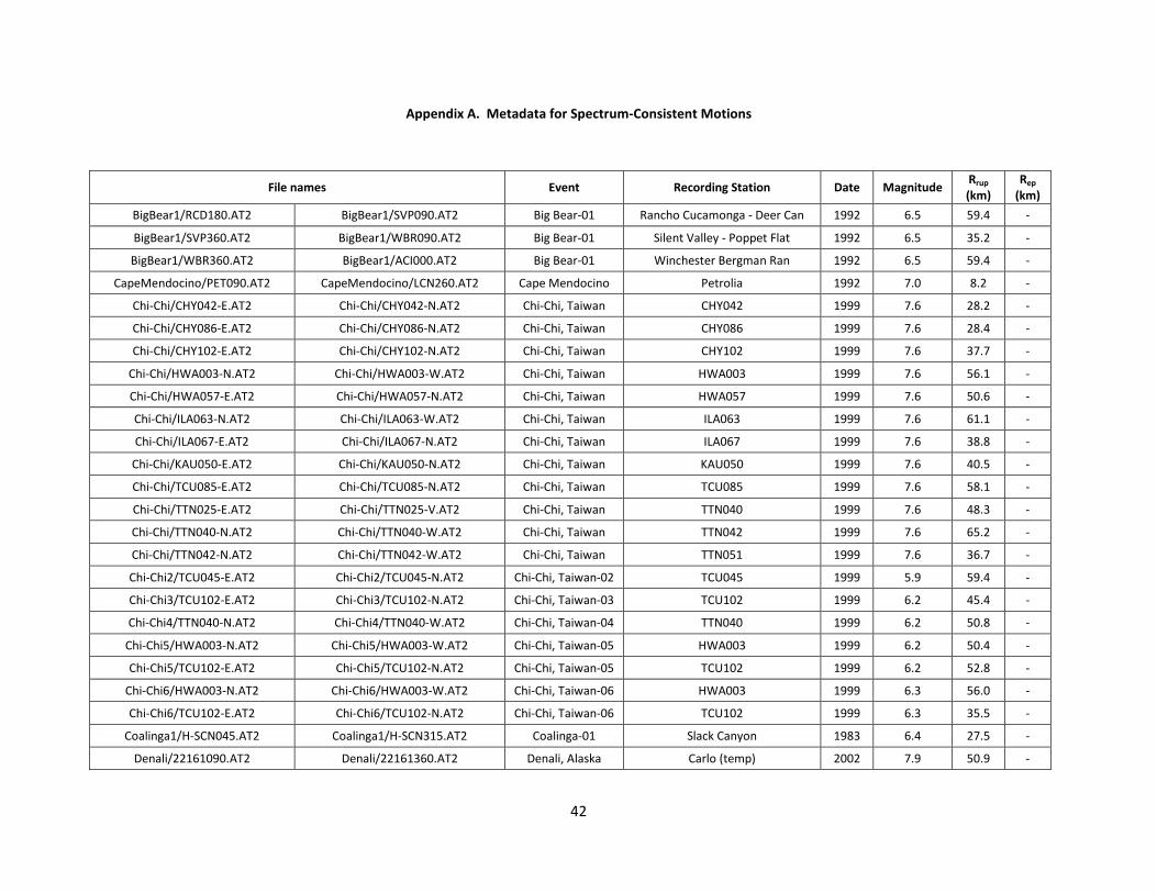
42
Appendix A. Metadata for Spectrum-Consistent Motions
File names Event Recording Station Date Magnitude Rrup
(km) Rep
(km)
BigBear1/RCD180.AT2 BigBear1/SVP090.AT2 Big Bear-01 Rancho Cucamonga - Deer Can 1992 6.5 59.4 -
BigBear1/SVP360.AT2 BigBear1/WBR090.AT2 Big Bear-01 Silent Valley - Poppet Flat 1992 6.5 35.2 -
BigBear1/WBR360.AT2 BigBear1/ACI000.AT2 Big Bear-01 Winchester Bergman Ran 1992 6.5 59.4 -
CapeMendocino/PET090.AT2 CapeMendocino/LCN260.AT2 Cape Mendocino Petrolia 1992 7.0 8.2 -
Chi-Chi/CHY042-E.AT2 Chi-Chi/CHY042-N.AT2 Chi-Chi, Taiwan CHY042 1999 7.6 28.2 -
Chi-Chi/CHY086-E.AT2 Chi-Chi/CHY086-N.AT2 Chi-Chi, Taiwan CHY086 1999 7.6 28.4 -
Chi-Chi/CHY102-E.AT2 Chi-Chi/CHY102-N.AT2 Chi-Chi, Taiwan CHY102 1999 7.6 37.7 -
Chi-Chi/HWA003-N.AT2 Chi-Chi/HWA003-W.AT2 Chi-Chi, Taiwan HWA003 1999 7.6 56.1 -
Chi-Chi/HWA057-E.AT2 Chi-Chi/HWA057-N.AT2 Chi-Chi, Taiwan HWA057 1999 7.6 50.6 -
Chi-Chi/ILA063-N.AT2 Chi-Chi/ILA063-W.AT2 Chi-Chi, Taiwan ILA063 1999 7.6 61.1 -
Chi-Chi/ILA067-E.AT2 Chi-Chi/ILA067-N.AT2 Chi-Chi, Taiwan ILA067 1999 7.6 38.8 -
Chi-Chi/KAU050-E.AT2 Chi-Chi/KAU050-N.AT2 Chi-Chi, Taiwan KAU050 1999 7.6 40.5 -
Chi-Chi/TCU085-E.AT2 Chi-Chi/TCU085-N.AT2 Chi-Chi, Taiwan TCU085 1999 7.6 58.1 -
Chi-Chi/TTN025-E.AT2 Chi-Chi/TTN025-V.AT2 Chi-Chi, Taiwan TTN040 1999 7.6 48.3 -
Chi-Chi/TTN040-N.AT2 Chi-Chi/TTN040-W.AT2 Chi-Chi, Taiwan TTN042 1999 7.6 65.2 -
Chi-Chi/TTN042-N.AT2 Chi-Chi/TTN042-W.AT2 Chi-Chi, Taiwan TTN051 1999 7.6 36.7 -
Chi-Chi2/TCU045-E.AT2 Chi-Chi2/TCU045-N.AT2 Chi-Chi, Taiwan-02 TCU045 1999 5.9 59.4 -
Chi-Chi3/TCU102-E.AT2 Chi-Chi3/TCU102-N.AT2 Chi-Chi, Taiwan-03 TCU102 1999 6.2 45.4 -
Chi-Chi4/TTN040-N.AT2 Chi-Chi4/TTN040-W.AT2 Chi-Chi, Taiwan-04 TTN040 1999 6.2 50.8 -
Chi-Chi5/HWA003-N.AT2 Chi-Chi5/HWA003-W.AT2 Chi-Chi, Taiwan-05 HWA003 1999 6.2 50.4 -
Chi-Chi5/TCU102-E.AT2 Chi-Chi5/TCU102-N.AT2 Chi-Chi, Taiwan-05 TCU102 1999 6.2 52.8 -
Chi-Chi6/HWA003-N.AT2 Chi-Chi6/HWA003-W.AT2 Chi-Chi, Taiwan-06 HWA003 1999 6.3 56.0 -
Chi-Chi6/TCU102-E.AT2 Chi-Chi6/TCU102-N.AT2 Chi-Chi, Taiwan-06 TCU102 1999 6.3 35.5 -
Coalinga1/H-SCN045.AT2 Coalinga1/H-SCN315.AT2 Coalinga-01 Slack Canyon 1983 6.4 27.5 -
Denali/22161090.AT2 Denali/22161360.AT2 Denali, Alaska Carlo (temp) 2002 7.9 50.9 -

43
Denali/5595-090.AT2 Denali/5596-090.AT2 Denali, Alaska R109 (temp) 2002 7.9 43.0 -
Geiyo/OIT013EW.AT2 Geiyo/OIT013NS.AT2 Geiyo OIT013 2001 6.4 - 154.0
Geiyo/YMG019EW.AT2 Geiyo/YMG019NS.AT2 Geiyo YMG019 2001 6.4 - 62.5
HectorMine/12647090.AT2 HectorMine/12647180.AT2 Hector Mine Twentynine Palms 1999 7.1 42.1 -
HectorMine/22T04090.AT2 HectorMine/22T04180.AT2 Hector Mine Hector 1999 7.1 11.7 -
HectorMine/HEC000.AT2 HectorMine/HEC090.AT2 Hector Mine Joshua Tree N.M. - Keys View 1999 7.1 50.4 -
HectorMine/vquez000.AT2 HectorMine/vquez090.AT2 Hector Mine Heart Bar State Park 1999 7.1 61.2 -
Hokkaido/HKD038EW.AT2 Hokkaido/HKD038NS.AT2 Hokkaido HKD038 2003 8.0 - 197.6
Irpinia1/A-ARI000.AT2 Irpinia1/A-ARI270.AT2 Irpinia, Italy-01 Arienzo 1980 6.9 52.9 -
Irpinia1/A-AUL000.AT2 Irpinia1/A-AUL270.AT2 Irpinia, Italy-01 Auletta 1980 6.9 9.6 -
Irpinia1/A-BAG000.AT2 Irpinia1/A-BAG270.AT2 Irpinia, Italy-01 Bagnoli Irpinio 1980 6.9 8.2 -
Irpinia1/A-BIS000.AT2 Irpinia1/A-BIS270.AT2 Irpinia, Italy-01 Bisaccia 1980 6.9 21.3 -
Irpinia2/B-AUL000.AT2 Irpinia2/B-AUL270.AT2 Irpinia, Italy-02 Auletta 1980 6.2 29.9 -
Irpinia2/B-STU000.AT2 Irpinia2/B-STU270.AT2 Irpinia, Italy-02 Sturno 1980 6.2 20.4 -
Iwaki/MYG011EW.AT2 Iwaki/MYG011NS.AT2 Iwaki MYG011 1998 5.4 - 157.0
Iwate1/MYG011EW.AT2 Iwate1/MYG011NS.AT2 Iwate1 MYG011 2001 6.4 - 124.2
Iwate2/MYG011EW.AT2 Iwate2/MYG011NS.AT2 Iwate2 MYG011 2008 6.8 - 159.1
JapanCoast/MYG011EW.AT2 JapanCoast/MYG011NS.AT2 JapanCoast MYG011 1999 5.5 - 81.3
JapanCoast2/MYG011EW.AT2 JapanCoast2/MYG011NS.AT2 JapanCoast2 MYG011 2000 5.0 - 34.2
JapanCoast3/MYG011EW.AT2 JapanCoast3/MYG011NS.AT2 JapanCoast3 MYG011 2001 5.4 - 68.9
JapanCoast4/MYG011EW.AT2 JapanCoast4/MYG011NS.AT2 JapanCoast4 MYG011 2002 6.1 - 86.4
JapanCoast5/MYG011EW.AT2 JapanCoast5/MYG011NS.AT2 JapanCoast5 MYG011 2003 6.2 - 31.5
JapanCoast6/MYG011EW.AT2 JapanCoast6/MYG011NS.AT2 JapanCoast6 MYG011 2010 5.5 - 77.0
Kagoshima/KMM014EW.AT2 Kagoshima/KMM014NS.AT2 Kagoshima KMM014 1997 6.2 - 70.1
Kocaeli/IZT090.AT2 Kocaeli/IZT180.AT2 Kocaeli, Turkey Izmit 1999 7.5 7.2 -
Kocaeli/MSK000.AT2 Kocaeli/MSK090.AT2 Kocaeli, Turkey Maslak 1999 7.5 55.3 -
KyushuM5.5/OIT013EW.AT2 KyushuM5.5/OIT013NS.AT2 KyushuM5.5 OIT013 2006 5.5 - 71.0
KyushuM5.7/OIT013EW.AT2 KyushuM5.7/OIT013NS.AT2 KyushuM5.7 OIT013 2002 5.7 - 76.0
KyushuM6.3/KMM014EW.AT2 KyushuM6.3/KMM014NS.AT2 KyushuM6.3 KMM014 1997 6.3 - 63.1
KyushuM6.6/OIT013EW.AT2 KyushuM6.6/OIT013NS.AT2 KyushuM6.6 OIT013 1996 6.6 - 144.4

44
Landers/29P090.AT2 Landers/RCD090.AT2 Landers Twentynine Palms 1992 7.3 41.4 -
Landers/LCN345.AT2 Landers/SIL000.AT2 Landers Lucerne 1992 7.3 2.2 -
Landers/SIL090.AT2 Landers/29P000.AT2 Landers Silent Valley - Poppet Flat 1992 7.3 50.9 -
LomaPrieta/CH09090.AT2 LomaPrieta/MCH000.AT2 Loma Prieta Lower Crystal Springs Dam dwnst 1989 6.9 48.4 -
LomaPrieta/G01000.AT2 LomaPrieta/G01090.AT2 Loma Prieta Gilroy Array #1 1989 6.9 9.6 -
LomaPrieta/GIL067.AT2 LomaPrieta/GIL337.AT2 Loma Prieta Gilroy - Gavilan Coll. 1989 6.9 10.0 -
LomaPrieta/LOB090.AT2 LomaPrieta/PET000.AT2 Loma Prieta UCSC Lick Observatory 1989 6.9 18.4 -
LomaPrieta/MCH090.AT2 LomaPrieta/PJH045.AT2 Loma Prieta Monterey City Hall 1989 6.9 44.4 -
LomaPrieta/PHT360.AT2 LomaPrieta/RIN000.AT2 Loma Prieta SF - Pacific Heights 1989 6.9 76.0 -
LomaPrieta/PJH315.AT2 LomaPrieta/SG3261.AT2 Loma Prieta Piedmont Jr High 1989 6.9 73.0 -
LomaPrieta/RIN090.AT2 LomaPrieta/TLH000.AT2 Loma Prieta SF - Rincon Hill 1989 6.9 74.1 -
LomaPrieta/SG3351.AT2 LomaPrieta/PHT270.AT2 Loma Prieta SAGO South - Surface 1989 6.9 34.3 -
LomaPrieta/SSF205.AT2 LomaPrieta/UC2000.AT2 Loma Prieta So. San Francisco, Sierra Pt. 1989 6.9 63.1 -
LomaPrieta/TLH090.AT2 LomaPrieta/SSF115.AT2 Loma Prieta SF - Telegraph Hill 1989 6.9 76.5 -
LomaPrieta/UC2090.AT2 LomaPrieta/LOB000.AT2 Loma Prieta UCSC 1989 6.9 18.5 -
MorganHill/LOB050.AT2 MorganHill/LOB320.AT2 Morgan Hill UCSC Lick Observatory 1984 6.2 45.5 -
MtFuji/OIT013EW.AT2 MtFuji/OIT013NS.AT2 MtFuji OIT013 2006 6.2 - 22.4
Nairiku/MYG011EW.AT2 Nairiku/MYG011NS.AT2 Nairiku MYG011 2008 7.2 - 97.0
Norcia/F-BEV-EW.AT2 Norcia/F-BEV-NS.AT2 Norcia, Italy Bevagna 1979 5.9 31.4 -
Northridge1/0141-360.AT2 Northridge1/WON095.AT2 Northridge-01 LA - Griffith Park Observatory 1994 6.7 23.8 -
Northridge1/5108-090.AT2 Northridge1/5108-360.AT2 Northridge-01 Santa Susana Ground 1994 6.7 16.7 -
Northridge1/ACI270.AT2 Northridge1/ATB000.AT2 Northridge-01 Anacapa Island 1994 6.7 68.9 -
Northridge1/ATB090.AT2 Northridge1/HOW060.AT2 Northridge-01 Antelope Buttes 1994 6.7 46.9 -
Northridge1/CHL160.AT2 Northridge1/0141-270.AT2 Northridge-01 LA - Chalon Rd 1994 6.7 20.4 -
Northridge1/HOW330.AT2 Northridge1/CHL070.AT2 Northridge-01 Burbank - Howard Rd. 1994 6.7 16.9 -
Northridge1/L04000.AT2 Northridge1/L04090.AT2 Northridge-01 Lake Hughes #4 - Camp Mend 1994 6.7 31.7 -
Northridge1/LA0090.AT2 Northridge1/L04-UP.AT2 Northridge-01 LA 00 1994 6.7 19.1 -
Northridge1/LIT090.AT2 Northridge1/LIT180.AT2 Northridge-01 Littlerock - Brainard Can 1994 6.7 46.6 -
Northridge1/LV1000.AT2 Northridge1/LV1090.AT2 Northridge-01 Leona Valley #1 1994 6.7 37.2 -
Northridge1/LV3000.AT2 Northridge1/LV3090.AT2 Northridge-01 Leona Valley #3 1994 6.7 37.3 -

45
Northridge1/MTW000.AT2 Northridge1/MTW090.AT2 Northridge-01 Mt Wilson - CIT Seis Sta 1994 6.7 35.9 -
Northridge1/PAC175.AT2 Northridge1/PAC265.AT2 Northridge-01 Pacoima Dam (downstr) 1994 6.7 7.0 -
Northridge1/PUL104.AT2 Northridge1/PUL194.AT2 Northridge-01 Pacoima Dam (upper left) 1994 6.7 7.0 -
Northridge1/SAN090.AT2 Northridge1/SAN180.AT2 Northridge-01 Sandberg - Bald Mtn 1994 6.7 41.6 -
Northridge1/VAS000.AT2 Northridge1/VAS090.AT2 Northridge-01 Vasquez Rocks Park 1994 6.7 23.6 -
Northridge1/WON185.AT2 Northridge1/LA0000.AT2 Northridge-01 LA - Wonderland Ave 1994 6.7 20.3 -
Northridge1/WWJ090.AT2 Northridge1/WWJ180.AT2 Northridge-01 Wrightwood - Jackson Flat 1994 6.7 64.7 -
Noto/GIF006EW.AT2 Noto/GIF006NS.AT2 Noto GIF006 2007 6.9 - 134.1
NPalmSprings/ARM270.AT2 NPalmSprings/ARM360.AT2 N. Palm Springs Anza - Red Mountain 1986 6.1 38.4 -
NPalmSprings/ARS270.AT2 NPalmSprings/ARS360.AT2 N. Palm Springs Santa Rosa Mountain 1986 6.1 39.1 -
NPalmSprings/ATL270.AT2 NPalmSprings/ATL360.AT2 N. Palm Springs Anza - Tule Canyon 1986 6.1 52.1 -
NPalmSprings/H01000.AT2 NPalmSprings/H01090.AT2 N. Palm Springs Murrieta Hot Springs 1986 6.1 54.8 -
NPalmSprings/H02000.AT2 NPalmSprings/H02090.AT2 N. Palm Springs Winchester Bergman Ran 1986 6.1 49.1 -
OshimaIsland/MYG011EW.AT2 OshimaIsland/MYG011NS.AT2 OshimaIsland MYG011 2003 7.0 - 58.8
PostTohuku/TCG016EW.AT2 PostTohuku/TCG016NS.AT2 PostTohuku TCG016 2011 7.1 - 63.7
PreTohuku/MYG011EW.AT2 PreTohuku/MYG011NS.AT2 PreTohuku MYG011 2010 6.7 - 70.3
SanFernando/FTR056.AT2 SanFernando/FTR326.AT2 San Fernando Fairmont Dam 1971 6.6 30.2 -
SanFernando/L04111.AT2 SanFernando/L04201.AT2 San Fernando Lake Hughes #4 1971 6.6 25.1 -
SanFernando/PUL164.AT2 SanFernando/PUL254.AT2 San Fernando Pacoima Dam (upper left abut) 1971 6.6 1.8 -
SanFernando/SAD003.AT2 SanFernando/SAD273.AT2 San Fernando Santa Anita Dam 1971 6.6 30.7 -
SierraMadre/212V5090.AT2 SierraMadre/212V5180.AT2 Sierra Madre Vasquez Rocks Park 1991 5.6 39.8 -
Sitka/TTN051-E.AT2 Sitka/TTN051-N.AT2 Sitka, Alaska Sitka Observatory 1972 7.7 34.6 -
Sukumo/OIT013EW.AT2 Sukumo/OIT013NS.AT2 Sukumo OIT013 2001 5.6 - 73.8
Tabas/TAB-LN.AT2 Tabas/TAB-TR.AT2 Tabas, Iran Tabas 1978 7.4 2.0 -
WhittierNarrows1/A-ANG000.AT2 WhittierNarrows1/A-ANG090.AT2 Whitt. Narrows-01 Mill Creek, Angeles Nat For 1987 6.0 36.8 -
WhittierNarrows1/A-CHL030.AT2 WhittierNarrows1/A-CHL120.AT2 Whitt. Narrows-01 LA - Chalon Rd 1987 6.0 35.2 -
WhittierNarrows1/A-VAS000.AT2 WhittierNarrows1/A-VAS090.AT2 Whitt. Narrows-01 Vasquez Rocks Park 1987 6.0 50.4 -
WhittierNarrows1/A-WON075.AT2 WhittierNarrows1/A-WON165.AT2 Whitt. Narrows-01 LA - Wonderland Ave 1987 6.0 27.6 -
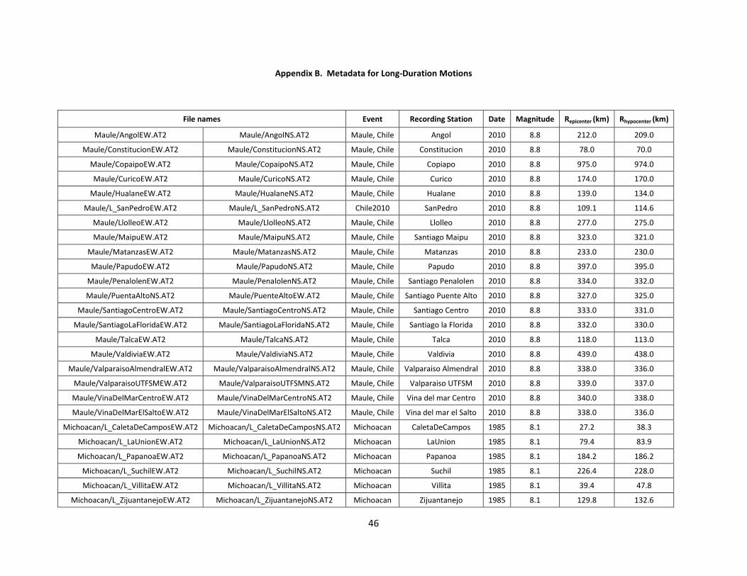
46
Appendix B. Metadata for Long-Duration Motions
File names Event Recording Station Date Magnitude Repicenter (km) Rhypocenter (km)
Maule/AngolEW.AT2 Maule/AngolNS.AT2 Maule, Chile Angol 2010 8.8 212.0 209.0
Maule/ConstitucionEW.AT2 Maule/ConstitucionNS.AT2 Maule, Chile Constitucion 2010 8.8 78.0 70.0
Maule/CopaipoEW.AT2 Maule/CopaipoNS.AT2 Maule, Chile Copiapo 2010 8.8 975.0 974.0
Maule/CuricoEW.AT2 Maule/CuricoNS.AT2 Maule, Chile Curico 2010 8.8 174.0 170.0
Maule/HualaneEW.AT2 Maule/HualaneNS.AT2 Maule, Chile Hualane 2010 8.8 139.0 134.0
Maule/L_SanPedroEW.AT2 Maule/L_SanPedroNS.AT2 Chile2010 SanPedro 2010 8.8 109.1 114.6
Maule/LlolleoEW.AT2 Maule/LlolleoNS.AT2 Maule, Chile Llolleo 2010 8.8 277.0 275.0
Maule/MaipuEW.AT2 Maule/MaipuNS.AT2 Maule, Chile Santiago Maipu 2010 8.8 323.0 321.0
Maule/MatanzasEW.AT2 Maule/MatanzasNS.AT2 Maule, Chile Matanzas 2010 8.8 233.0 230.0
Maule/PapudoEW.AT2 Maule/PapudoNS.AT2 Maule, Chile Papudo 2010 8.8 397.0 395.0
Maule/PenalolenEW.AT2 Maule/PenalolenNS.AT2 Maule, Chile Santiago Penalolen 2010 8.8 334.0 332.0
Maule/PuentaAltoNS.AT2 Maule/PuenteAltoEW.AT2 Maule, Chile Santiago Puente Alto 2010 8.8 327.0 325.0
Maule/SantiagoCentroEW.AT2 Maule/SantiagoCentroNS.AT2 Maule, Chile Santiago Centro 2010 8.8 333.0 331.0
Maule/SantiagoLaFloridaEW.AT2 Maule/SantiagoLaFloridaNS.AT2 Maule, Chile Santiago la Florida 2010 8.8 332.0 330.0
Maule/TalcaEW.AT2 Maule/TalcaNS.AT2 Maule, Chile Talca 2010 8.8 118.0 113.0
Maule/ValdiviaEW.AT2 Maule/ValdiviaNS.AT2 Maule, Chile Valdivia 2010 8.8 439.0 438.0
Maule/ValparaisoAlmendralEW.AT2 Maule/ValparaisoAlmendralNS.AT2 Maule, Chile Valparaiso Almendral 2010 8.8 338.0 336.0
Maule/ValparaisoUTFSMEW.AT2 Maule/ValparaisoUTFSMNS.AT2 Maule, Chile Valparaiso UTFSM 2010 8.8 339.0 337.0
Maule/VinaDelMarCentroEW.AT2 Maule/VinaDelMarCentroNS.AT2 Maule, Chile Vina del mar Centro 2010 8.8 340.0 338.0
Maule/VinaDelMarElSaltoEW.AT2 Maule/VinaDelMarElSaltoNS.AT2 Maule, Chile Vina del mar el Salto 2010 8.8 338.0 336.0
Michoacan/L_CaletaDeCamposEW.AT2 Michoacan/L_CaletaDeCamposNS.AT2 Michoacan CaletaDeCampos 1985 8.1 27.2 38.3
Michoacan/L_LaUnionEW.AT2 Michoacan/L_LaUnionNS.AT2 Michoacan LaUnion 1985 8.1 79.4 83.9
Michoacan/L_PapanoaEW.AT2 Michoacan/L_PapanoaNS.AT2 Michoacan Papanoa 1985 8.1 184.2 186.2
Michoacan/L_SuchilEW.AT2 Michoacan/L_SuchilNS.AT2 Michoacan Suchil 1985 8.1 226.4 228.0
Michoacan/L_VillitaEW.AT2 Michoacan/L_VillitaNS.AT2 Michoacan Villita 1985 8.1 39.4 47.8
Michoacan/L_ZijuantanejoEW.AT2 Michoacan/L_ZijuantanejoNS.AT2 Michoacan Zijuantanejo 1985 8.1 129.8 132.6

47
Peru1966/L_Arequipa008.AT2 Peru1966/L_Arequipa282.AT2 Peru1966 Island 1966 8.0 237.0 240.0
SumatraFS/L_WestSumatraEW.AT2 SumatraFS/L_WestSumatraNS.AT2 SumatraFS Sikuai 2007 7.9 164.6 167.3
Tohuku/L_AOM007EW.AT2 Tohuku/L_AOM007NS.AT2 Tohuku AOM007 2011 9.0 381.2 381.9
Tohuku/L_CHB002EW.AT2 Tohuku/L_CHB002NS.AT2 Tohuku CHB002 2011 9.0 362.8 363.6
Tohuku/L_CHB004EW.AT2 Tohuku/L_CHB004NS.AT2 Tohuku CHB004 2011 9.0 316.8 317.7
Tohuku/L_CHB012EW.AT2 Tohuku/L_CHB012NS.AT2 Tohuku CHB012 2011 9.0 353.7 354.5
Tohuku/L_CHB028EW.AT2 Tohuku/L_CHB028NS.AT2 Tohuku CHB028 2011 9.0 360.3 361.1
Tohuku/L_FKS001EW.AT2 Tohuku/L_FKS001NS.AT2 Tohuku FKS001 2011 9.0 175.3 176.9
Tohuku/L_FKS002EW.AT2 Tohuku/L_FKS002NS.AT2 Tohuku FKS002 2011 9.0 202.4 203.8
Tohuku/L_FKS003EW.AT2 Tohuku/L_FKS003NS.AT2 Tohuku FKS003 2011 9.0 214.1 215.4
Tohuku/L_FKS004EW.AT2 Tohuku/L_FKS004NS.AT2 Tohuku FKS004 2011 9.0 193.5 195.0
Tohuku/L_FKS006EW.AT2 Tohuku/L_FKS006NS.AT2 Tohuku FKS006 2011 9.0 196.2 197.7
Tohuku/L_FKS011EW.AT2 Tohuku/L_FKS011NS.AT2 Tohuku FKS011 2011 9.0 203.0 204.4
Tohuku/L_FKS012EW.AT2 Tohuku/L_FKS012NS.AT2 Tohuku FKS012 2011 9.0 222.2 223.5
Tohuku/L_FKS013EW.AT2 Tohuku/L_FKS013NS.AT2 Tohuku FKS013 2011 9.0 230.1 231.4
Tohuku/L_FKS014EW.AT2 Tohuku/L_FKS014NS.AT2 Tohuku FKS014 2011 9.0 251.8 253.0
Tohuku/L_FKS015EW.AT2 Tohuku/L_FKS015NS.AT2 Tohuku FKS015 2011 9.0 247.7 248.9
Tohuku/L_FKS017EW.AT2 Tohuku/L_FKS017NS.AT2 Tohuku FKS017 2011 9.0 236.7 237.9
Tohuku/L_FKS019EW.AT2 Tohuku/L_FKS019NS.AT2 Tohuku FKS019 2011 9.0 220.9 222.2
Tohuku/L_FKS020EW.AT2 Tohuku/L_FKS020NS.AT2 Tohuku FKS020 2011 9.0 250.5 251.7
Tohuku/L_FKS023EW.AT2 Tohuku/L_FKS023NS.AT2 Tohuku FKS023 2011 9.0 267.6 268.7
Tohuku/L_FKS024EW.AT2 Tohuku/L_FKS024NS.AT2 Tohuku FKS024 2011 9.0 252.6 253.8
Tohuku/L_FKS031EW.AT2 Tohuku/L_FKS031NS.AT2 Tohuku FKS031 2011 9.0 198.0 199.5
Tohuku/L_GNM009EW.AT2 Tohuku/L_GNM009NS.AT2 Tohuku GNM009 2011 9.0 362.6 363.4
Tohuku/L_IBR001EW.AT2 Tohuku/L_IBR001NS.AT2 Tohuku IBR001 2011 9.0 262.7 263.8
Tohuku/L_IBR002EW.AT2 Tohuku/L_IBR002NS.AT2 Tohuku IBR002 2011 9.0 241.4 242.6
Tohuku/L_IBR006EW.AT2 Tohuku/L_IBR006NS.AT2 Tohuku IBR006 2011 9.0 282.7 283.7
Tohuku/L_IBR007EW.AT2 Tohuku/L_IBR007NS.AT2 Tohuku IBR007 2011 9.0 274.4 275.4
Tohuku/L_IBR008EW.AT2 Tohuku/L_IBR008NS.AT2 Tohuku IBR008 2011 9.0 319.9 320.8
Tohuku/L_IBR010EW.AT2 Tohuku/L_IBR010NS.AT2 Tohuku IBR010 2011 9.0 329.4 330.3

48
Tohuku/L_IBR011EW.AT2 Tohuku/L_IBR011NS.AT2 Tohuku IBR011 2011 9.0 325.0 325.9
Tohuku/L_IBR012EW.AT2 Tohuku/L_IBR012NS.AT2 Tohuku IBR012 2011 9.0 307.0 307.9
Tohuku/L_IBR014EW.AT2 Tohuku/L_IBR014NS.AT2 Tohuku IBR014 2011 9.0 321.9 322.8
Tohuku/L_IBR017EW.AT2 Tohuku/L_IBR017NS.AT2 Tohuku IBR017 2011 9.0 323.0 323.9
Tohuku/L_IBR018EW.AT2 Tohuku/L_IBR018NS.AT2 Tohuku IBR018 2011 9.0 302.0 302.9
Tohuku/L_IWT001EW.AT2 Tohuku/L_IWT001NS.AT2 Tohuku IWT001 2011 9.0 286.7 287.7
Tohuku/L_IWT005EW.AT2 Tohuku/L_IWT005NS.AT2 Tohuku IWT005 2011 9.0 201.0 202.4
Tohuku/L_IWT009EW.AT2 Tohuku/L_IWT009NS.AT2 Tohuku IWT009 2011 9.0 172.6 174.3
Tohuku/L_IWT011EW.AT2 Tohuku/L_IWT011NS.AT2 Tohuku IWT011 2011 9.0 198.3 199.8
Tohuku/L_IWT012EW.AT2 Tohuku/L_IWT012NS.AT2 Tohuku IWT012 2011 9.0 212.1 213.5
Tohuku/L_IWT013EW.AT2 Tohuku/L_IWT013NS.AT2 Tohuku IWT013 2011 9.0 190.0 191.5
Tohuku/L_IWT017EW.AT2 Tohuku/L_IWT017NS.AT2 Tohuku IWT017 2011 9.0 221.5 222.9
Tohuku/L_IWT018EW.AT2 Tohuku/L_IWT018NS.AT2 Tohuku IWT018 2011 9.0 242.0 243.2
Tohuku/L_IWT019EW.AT2 Tohuku/L_IWT019NS.AT2 Tohuku IWT019 2011 9.0 226.5 227.8
Tohuku/L_IWT020EW.AT2 Tohuku/L_IWT020NS.AT2 Tohuku IWT020 2011 9.0 240.5 241.8
Tohuku/L_IWT021EW.AT2 Tohuku/L_IWT021NS.AT2 Tohuku IWT021 2011 9.0 265.2 266.3
Tohuku/L_IWT026EW.AT2 Tohuku/L_IWT026NS.AT2 Tohuku IWT026 2011 9.0 209.9 211.2
Tohuku/L_MYG001EW.AT2 Tohuku/L_MYG001NS.AT2 Tohuku MYG001 2011 9.0 153.3 155.2
Tohuku/L_MYG005EW.AT2 Tohuku/L_MYG005NS.AT2 Tohuku MYG005 2011 9.0 215.2 216.6
Tohuku/L_MYG006EW.AT2 Tohuku/L_MYG006NS.AT2 Tohuku MYG006 2011 9.0 180.8 182.4
Tohuku/L_MYG007EW.AT2 Tohuku/L_MYG007NS.AT2 Tohuku MYG007 2011 9.0 158.1 159.9
Tohuku/L_MYG008EW.AT2 Tohuku/L_MYG008NS.AT2 Tohuku MYG008 2011 9.0 141.8 143.8
Tohuku/L_MYG009EW.AT2 Tohuku/L_MYG009NS.AT2 Tohuku MYG009 2011 9.0 182.7 184.3
Tohuku/L_MYG010EW.AT2 Tohuku/L_MYG010NS.AT2 Tohuku MYG010 2011 9.0 149.3 151.2
Tohuku/L_MYG014EW.AT2 Tohuku/L_MYG014NS.AT2 Tohuku MYG014 2011 9.0 201.1 202.6
Tohuku/L_MYG015EW.AT2 Tohuku/L_MYG015NS.AT2 Tohuku MYG015 2011 9.0 178.2 179.8
Tohuku/L_MYG016EW.AT2 Tohuku/L_MYG016NS.AT2 Tohuku MYG016 2011 9.0 199.7 201.2
Tohuku/L_MYG017EW.AT2 Tohuku/L_MYG017NS.AT2 Tohuku MYG017 2011 9.0 185.7 187.2
Tohuku/L_SIT004EW.AT2 Tohuku/L_SIT004NS.AT2 Tohuku SIT004 2011 9.0 396.5 397.3
Tohuku/L_TCG001EW.AT2 Tohuku/L_TCG001NS.AT2 Tohuku TCG001 2011 9.0 275.1 276.2

49
Tohuku/L_TCG003EW.AT2 Tohuku/L_TCG003NS.AT2 Tohuku TCG003 2011 9.0 310.7 311.6
Tohuku/L_TCG004EW.AT2 Tohuku/L_TCG004NS.AT2 Tohuku TCG004 2011 9.0 334.8 335.8
Tohuku/L_TCG005EW.AT2 Tohuku/L_TCG005NS.AT2 Tohuku TCG005 2011 9.0 294.3 295.3
Tohuku/L_TCG006EW.AT2 Tohuku/L_TCG006NS.AT2 Tohuku TCG006 2011 9.0 280.7 281.8
Tohuku/L_TCG008EW.AT2 Tohuku/L_TCG008NS.AT2 Tohuku TCG008 2011 9.0 320.1 321.0
Tohuku/L_TCG012EW.AT2 Tohuku/L_TCG012NS.AT2 Tohuku TCG012 2011 9.0 334.1 334.9
Tohuku/L_TCG013EW.AT2 Tohuku/L_TCG013NS.AT2 Tohuku TCG013 2011 9.0 308.5 309.4
Tohuku/L_TCG016EW.AT2 Tohuku/L_TCG016NS.AT2 Tohuku TCG016 2011 9.0 292.8 293.8
Tohuku/L_TKY017EW.AT2 Tohuku/L_TKY017NS.AT2 Tohuku TKY017 2011 9.0 379.6 380.4
Tohuku/L_TKY026EW.AT2 Tohuku/L_TKY026NS.AT2 Tohuku TKY026 2011 9.0 374.4 375.1
Tohuku/L_YMT006EW.AT2 Tohuku/L_YMT006NS.AT2 Tohuku YMT006 2011 9.0 227.7 229.0
Valparaiso/L_Cauquenes-EW.AT2 Valparaiso/L_Cauquenes-NS.AT2 Valparaiso Cauquenes 1985 7.8 320.0 321.7
Valparaiso/L_Constitucion-EW.AT2 Valparaiso/L_Constitucion-NS.AT2 Valparaiso Cotitucion 1985 7.8 233.3 235.7
Valparaiso/L_Endesa-EW.AT2 Valparaiso/L_Endesa-NS.AT2 Valparaiso Endesa 1985 7.8 - -
Valparaiso/L_Hualane-EW.AT2 Valparaiso/L_Hualane-NS.AT2 Valparaiso Hualane 1985 7.8 204.1 206.8
Valparaiso/L_Illapel-340.AT2 Valparaiso/L_Illapel-70.AT2 Valparaiso Illapel 1985 7.8 179.9 182.9
Valparaiso/L_Iloca-EW.AT2 Valparaiso/L_Iloca-NS.AT2 Valparaiso Iloca 1985 7.8 201.1 203.8
Valparaiso/L_Laligua-290.AT2 Valparaiso/L_Laligue-200.AT2 Valparaiso Laligua 1985 7.8 95.5 101.0
Valparaiso/L_Llayllay-190.AT2 Valparaiso/L_Llayllay-280.AT2 Valparaiso Llayllay 1985 7.8 89.8 95.6
Valparaiso/L_Llolleo-010.AT2 Valparaiso/L_Llolleo-100.AT2 Valparaiso Llolleo 1985 7.8 60.0 68.5
Valparaiso/L_LosVilos-EW.AT2 Valparaiso/L_LosVilos-NS.AT2 Valparaiso LosVilos 1985 7.8 139.5 143.4
Valparaiso/L_Melipilla-EW.AT2 Valparaiso/L_Melipilla-NS.AT2 Valparaiso Melipilla 1985 7.8 85.6 91.7
Valparaiso/L_Papudo-140.AT2 Valparaiso Papudo 1985 7.8 79.9 86.4
Valparaiso/L_Pichilemu-EW.AT2 Valparaiso/L_Pichilemu-NS.AT2 Valparaiso Pichilemu 1985 7.8 139.1 143.0
Valparaiso/L_Quintay-EW.AT2 Valparaiso/L_Quintay-NS.AT2 Valparaiso Quintay 1985 7.8 53.4 62.8
Valparaiso/L_Rapel-EW.AT2 Valparaiso/L_Rapel-NS.AT2 Valparaiso Rapel 1985 7.8 103.0 108.2
Valparaiso/L_SanFelipe-080.AT2 Valparaiso/L_SanFelipe-170.AT2 Valparaiso SanFelipe 1985 7.8 114.8 119.4
Valparaiso/L_SanFern-EW.AT2 Valparaiso/L_SanFern-NS.AT2 Valparaiso SanFern 1985 7.8 181.7 184.7
Valparaiso/L_SanIsidroEW.AT2 Valparaiso/L_SanIsidro-NS.AT2 Valparaiso SanIsidro 1985 7.8 - -
Valparaiso/L_Talca-010.AT2 Valparaiso/L_Talca-280.AT2 Valparaiso Talca 1985 7.8 222.3 224.7

50
Valparaiso/L_ValElAlm-050.AT2 Valparaiso/L_ValElAlm-140.AT2 Valparaiso ValElAlm 1985 7.8 25.8 41.9
Valparaiso/L_ValpoUFSM-160.AT2 Valparaiso/L_ValpoUFSM-070.AT2 Valparaiso ValopUFSM 1985 7.8 124.9 129.2
Valparaiso/L_Ventanas-EW.AT2 Valparaiso/L_Ventanas-NS.AT2 Valparaiso Ventanas 1985 7.8 26.1 42.1
Valparaiso/L_Vina-200.AT2 Valparaiso/L_Vina-290.AT2 Valparaiso Vina 1985 7.8 30.8 45.2
Valparaiso/L_Zapallar-EW.AT2 Valparaiso/L_Zapallar-NS.AT2 Valparaiso Zapallar 1985 7.8 73.2 80.3
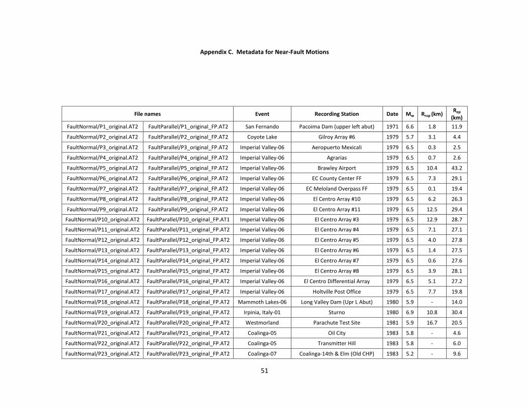
51
Appendix C. Metadata for Near-Fault Motions
File names Event Recording Station Date Mw Rrup (km) Rep
(km)
FaultNormal/P1_original.AT2 FaultParallel/P1_original_FP.AT2 San Fernando Pacoima Dam (upper left abut) 1971 6.6 1.8 11.9
FaultNormal/P2_original.AT2 FaultParallel/P2_original_FP.AT2 Coyote Lake Gilroy Array #6 1979 5.7 3.1 4.4
FaultNormal/P3_original.AT2 FaultParallel/P3_original_FP.AT2 Imperial Valley-06 Aeropuerto Mexicali 1979 6.5 0.3 2.5
FaultNormal/P4_original.AT2 FaultParallel/P4_original_FP.AT2 Imperial Valley-06 Agrarias 1979 6.5 0.7 2.6
FaultNormal/P5_original.AT2 FaultParallel/P5_original_FP.AT2 Imperial Valley-06 Brawley Airport 1979 6.5 10.4 43.2
FaultNormal/P6_original.AT2 FaultParallel/P6_original_FP.AT2 Imperial Valley-06 EC County Center FF 1979 6.5 7.3 29.1
FaultNormal/P7_original.AT2 FaultParallel/P7_original_FP.AT2 Imperial Valley-06 EC Meloland Overpass FF 1979 6.5 0.1 19.4
FaultNormal/P8_original.AT2 FaultParallel/P8_original_FP.AT2 Imperial Valley-06 El Centro Array #10 1979 6.5 6.2 26.3
FaultNormal/P9_original.AT2 FaultParallel/P9_original_FP.AT2 Imperial Valley-06 El Centro Array #11 1979 6.5 12.5 29.4
FaultNormal/P10_original.AT2 FaultParallel/P10_original_FP.AT1 Imperial Valley-06 El Centro Array #3 1979 6.5 12.9 28.7
FaultNormal/P11_original.AT2 FaultParallel/P11_original_FP.AT2 Imperial Valley-06 El Centro Array #4 1979 6.5 7.1 27.1
FaultNormal/P12_original.AT2 FaultParallel/P12_original_FP.AT2 Imperial Valley-06 El Centro Array #5 1979 6.5 4.0 27.8
FaultNormal/P13_original.AT2 FaultParallel/P13_original_FP.AT2 Imperial Valley-06 El Centro Array #6 1979 6.5 1.4 27.5
FaultNormal/P14_original.AT2 FaultParallel/P14_original_FP.AT2 Imperial Valley-06 El Centro Array #7 1979 6.5 0.6 27.6
FaultNormal/P15_original.AT2 FaultParallel/P15_original_FP.AT2 Imperial Valley-06 El Centro Array #8 1979 6.5 3.9 28.1
FaultNormal/P16_original.AT2 FaultParallel/P16_original_FP.AT2 Imperial Valley-06 El Centro Differential Array 1979 6.5 5.1 27.2
FaultNormal/P17_original.AT2 FaultParallel/P17_original_FP.AT2 Imperial Valley-06 Holtville Post Office 1979 6.5 7.7 19.8
FaultNormal/P18_original.AT2 FaultParallel/P18_original_FP.AT2 Mammoth Lakes-06 Long Valley Dam (Upr L Abut) 1980 5.9 - 14.0
FaultNormal/P19_original.AT2 FaultParallel/P19_original_FP.AT2 Irpinia, Italy-01 Sturno 1980 6.9 10.8 30.4
FaultNormal/P20_original.AT2 FaultParallel/P20_original_FP.AT2 Westmorland Parachute Test Site 1981 5.9 16.7 20.5
FaultNormal/P21_original.AT2 FaultParallel/P21_original_FP.AT2 Coalinga-05 Oil City 1983 5.8 - 4.6
FaultNormal/P22_original.AT2 FaultParallel/P22_original_FP.AT2 Coalinga-05 Transmitter Hill 1983 5.8 - 6.0
FaultNormal/P23_original.AT2 FaultParallel/P23_original_FP.AT2 Coalinga-07 Coalinga-14th & Elm (Old CHP) 1983 5.2 - 9.6

52
FaultNormal/P24_original.AT2 FaultParallel/P24_original_FP.AT2 Morgan Hill Coyote Lake Dam (SW Abut) 1984 6.2 0.5 24.6
FaultNormal/P25_original.AT2 FaultParallel/P25_original_FP.AT2 Morgan Hill Gilroy Array #6 1984 6.2 9.9 36.3
FaultNormal/P26_original.AT2 FaultParallel/P26_original_FP.AT2 Taiwan SMART1(40) SMART1 C00 1986 6.3 - 68.2
FaultNormal/P27_original.AT2 FaultParallel/P27_original_FP.AT2 Taiwan SMART1(40) SMART1 M07 1986 6.3 - 67.2
FaultNormal/P28_original.AT2 FaultParallel/P28_original_FP.AT2 N. Palm Springs North Palm Springs 1986 6.1 4.0 10.6
FaultNormal/P29_original.AT2 FaultParallel/P29_original_FP.AT2 San Salvador Geotech Investig Center 1986 5.8 6.3 7.9
FaultNormal/P30_original.AT2 FaultParallel/P30_original_FP.AT2 Whittier Narrows-01 Downey - Co Maint Bldg 1987 6.0 20.8 16.0
FaultNormal/P31_original.AT2 FaultParallel/P31_original_FP.AT2 Whittier Narrows-01 LB - Orange Ave 1987 6.0 24.5 20.7
FaultNormal/P32_original.AT2 FaultParallel/P32_original_FP.AT2 Superstition Hills-02 Parachute Test Site 1987 6.5 1.0 16.0
FaultNormal/P33_original.AT2 FaultParallel/P33_original_FP.AT2 Loma Prieta Alameda Naval Air Stn Hanger 1989 6.9 71.0 90.8
FaultNormal/P34_original.AT2 FaultParallel/P34_original_FP.AT2 Loma Prieta Gilroy Array #2 1989 6.9 11.1 29.8
FaultNormal/P35_original.AT2 FaultParallel/P35_original_FP.AT2 Loma Prieta Oakland - Outer Harbor Wharf 1989 6.9 74.3 94.0
FaultNormal/P36_original.AT2 FaultParallel/P36_original_FP.AT2 Loma Prieta Saratoga - Aloha Ave 1989 6.9 8.5 27.2
FaultNormal/P37_original.AT2 FaultParallel/P37_original_FP.AT2 Erzican, Turkey Erzincan 1992 6.7 4.4 9.0
FaultNormal/P38_original.AT2 FaultParallel/P38_original_FP.AT2 Cape Mendocino Petrolia 1992 7.0 8.2 4.5
FaultNormal/P39_original.AT2 FaultParallel/P39_original_FP.AT2 Landers Barstow 1992 7.3 34.9 94.8
FaultNormal/P40_original.AT2 FaultParallel/P40_original_FP.AT2 Landers Lucerne 1992 7.3 2.2 44.0
FaultNormal/P41_original.AT2 FaultParallel/P41_original_FP.AT2 Landers Yermo Fire Station 1992 7.3 23.6 86.0
FaultNormal/P42_original.AT2 FaultParallel/P42_original_FP.AT2 Northridge-01 Jensen Filter Plant 1994 6.7 5.4 13.0
FaultNormal/P43_original.AT2 FaultParallel/P43_original_FP.AT2 Northridge-01 Jensen Filter Plant Generator 1994 6.7 5.4 13.0
FaultNormal/P44_original.AT2 FaultParallel/P44_original_FP.AT2 Northridge-01 LA - Wadsworth VA Hospital North 1994 6.7 23.6 19.6
FaultNormal/P45_original.AT2 FaultParallel/P45_original_FP.AT2 Northridge-01 LA Dam 1994 6.7 5.9 11.8
FaultNormal/P46_original.AT2 FaultParallel/P46_original_FP.AT2 Northridge-01 Newhall - W Pico Canyon Rd. 1994 6.7 5.5 21.6
FaultNormal/P47_original.AT2 FaultParallel/P47_original_FP.AT2 Northridge-01 Pacoima Dam (downstr) 1994 6.7 7.0 20.4
FaultNormal/P48_original.AT2 FaultParallel/P48_original_FP.AT2 Northridge-01 Pacoima Dam (upper left) 1994 6.7 7.0 20.4
FaultNormal/P49_original.AT2 FaultParallel/P49_original_FP.AT2 Northridge-01 Rinaldi Receiving Sta 1994 6.7 6.5 10.9
FaultNormal/P50_original.AT2 FaultParallel/P50_original_FP.AT2 Northridge-01 Sylmar - Converter Sta 1994 6.7 5.4 13.1
FaultNormal/P51_original.AT2 FaultParallel/P51_original_FP.AT2 Northridge-01 Sylmar - Converter Sta East 1994 6.7 5.2 13.6
FaultNormal/P52_original.AT2 FaultParallel/P52_original_FP.AT2 Northridge-01 Sylmar - Olive View Med FF 1994 6.7 5.3 16.8
FaultNormal/P53_original.AT2 FaultParallel/P53_original_FP.AT2 Kobe, Japan Takarazuka 1995 6.9 0.3 38.6

53
FaultNormal/P54_original.AT2 FaultParallel/P54_original_FP.AT2 Kobe, Japan Takatori 1995 6.9 1.5 13.1
FaultNormal/P55_original.AT2 FaultParallel/P55_original_FP.AT2 Kocaeli, Turkey Gebze 1999 7.5 10.9 47.0
FaultNormal/P56_original.AT2 FaultParallel/P56_original_FP.AT2 Chi-Chi, Taiwan CHY006 1999 7.6 9.8 40.5
FaultNormal/P57_original.AT2 FaultParallel/P57_original_FP.AT2 Chi-Chi, Taiwan CHY035 1999 7.6 12.7 43.9
FaultNormal/P58_original.AT2 FaultParallel/P58_original_FP.AT2 Chi-Chi, Taiwan CHY101 1999 7.6 10.0 32.0
FaultNormal/P59_original.AT2 FaultParallel/P59_original_FP.AT2 Chi-Chi, Taiwan TAP003 1999 7.6 102.4 151.7
FaultNormal/P60_original.AT2 FaultParallel/P60_original_FP.AT2 Chi-Chi, Taiwan TCU029 1999 7.6 28.1 79.2
FaultNormal/P61_original.AT2 FaultParallel/P61_original_FP.AT2 Chi-Chi, Taiwan TCU031 1999 7.6 30.2 80.1
FaultNormal/P62_original.AT2 FaultParallel/P62_original_FP.AT2 Chi-Chi, Taiwan TCU034 1999 7.6 35.7 87.9
FaultNormal/P63_original.AT2 FaultParallel/P63_original_FP.AT2 Chi-Chi, Taiwan TCU036 1999 7.6 19.8 67.8
FaultNormal/P64_original.AT2 FaultParallel/P64_original_FP.AT2 Chi-Chi, Taiwan TCU038 1999 7.6 25.4 73.1
FaultNormal/P65_original.AT2 FaultParallel/P65_original_FP.AT2 Chi-Chi, Taiwan TCU040 1999 7.6 22.1 69.0
FaultNormal/P66_original.AT2 FaultParallel/P66_original_FP.AT2 Chi-Chi, Taiwan TCU042 1999 7.6 26.3 78.4
FaultNormal/P67_original.AT2 FaultParallel/P67_original_FP.AT2 Chi-Chi, Taiwan TCU046 1999 7.6 16.7 68.9
FaultNormal/P68_original.AT2 FaultParallel/P68_original_FP.AT2 Chi-Chi, Taiwan TCU049 1999 7.6 3.8 38.9
FaultNormal/P69_original.AT2 FaultParallel/P69_original_FP.AT2 Chi-Chi, Taiwan TCU053 1999 7.6 6.0 41.2
FaultNormal/P70_original.AT2 FaultParallel/P70_original_FP.AT2 Chi-Chi, Taiwan TCU054 1999 7.6 5.3 37.6
FaultNormal/P71_original.AT2 FaultParallel/P71_original_FP.AT2 Chi-Chi, Taiwan TCU056 1999 7.6 10.5 39.7
FaultNormal/P72_original.AT2 FaultParallel/P72_original_FP.AT2 Chi-Chi, Taiwan TCU060 1999 7.6 8.5 45.4
FaultNormal/P73_original.AT2 FaultParallel/P73_original_FP.AT2 Chi-Chi, Taiwan TCU065 1999 7.6 0.6 26.7
FaultNormal/P74_original.AT2 FaultParallel/P74_original_FP.AT2 Chi-Chi, Taiwan TCU068 1999 7.6 0.3 47.9
FaultNormal/P75_original.AT2 FaultParallel/P75_original_FP.AT2 Chi-Chi, Taiwan TCU075 1999 7.6 0.9 20.7
FaultNormal/P76_original.AT2 FaultParallel/P76_original_FP.AT2 Chi-Chi, Taiwan TCU076 1999 7.6 2.8 16.0
FaultNormal/P77_original.AT2 FaultParallel/P77_original_FP.AT2 Chi-Chi, Taiwan TCU082 1999 7.6 5.2 36.2
FaultNormal/P78_original.AT2 FaultParallel/P78_original_FP.AT2 Chi-Chi, Taiwan TCU087 1999 7.6 7.0 55.6
FaultNormal/P79_original.AT2 FaultParallel/P79_original_FP.AT2 Chi-Chi, Taiwan TCU098 1999 7.6 47.7 99.7
FaultNormal/P80_original.AT2 FaultParallel/P80_original_FP.AT2 Chi-Chi, Taiwan TCU101 1999 7.6 2.1 45.1
FaultNormal/P81_original.AT2 FaultParallel/P81_original_FP.AT2 Chi-Chi, Taiwan TCU102 1999 7.6 1.5 45.6
FaultNormal/P82_original.AT2 FaultParallel/P82_original_FP.AT2 Chi-Chi, Taiwan TCU103 1999 7.6 6.1 52.4
FaultNormal/P83_original.AT2 FaultParallel/P83_original_FP.AT2 Chi-Chi, Taiwan TCU104 1999 7.6 12.9 49.3

54
FaultNormal/P84_original.AT2 FaultParallel/P84_original_FP.AT2 Chi-Chi, Taiwan TCU128 1999 7.6 13.2 63.3
FaultNormal/P85_original.AT2 FaultParallel/P85_original_FP.AT2 Chi-Chi, Taiwan TCU136 1999 7.6 8.3 48.8
FaultNormal/P86_original.AT2 FaultParallel/P86_original_FP.AT2 Northwest China-03 Jiashi 1997 6.1 - 19.1
FaultNormal/P87_original.AT2 FaultParallel/P87_original_FP.AT2 Yountville Napa Fire Station #3 2000 5.0 - 9.9
FaultNormal/P88_original.AT2 FaultParallel/P88_original_FP.AT2 Chi-Chi, Taiwan-03 CHY024 1999 6.2 19.7 25.5
FaultNormal/P89_original.AT2 FaultParallel/P89_original_FP.AT2 Chi-Chi, Taiwan-03 CHY080 1999 6.2 22.4 29.5
FaultNormal/P90_original.AT2 FaultParallel/P90_original_FP.AT2 Chi-Chi, Taiwan-03 TCU076 1999 6.2 14.7 20.8
FaultNormal/P91_original.AT2 FaultParallel/P91_original_FP.AT2 Chi-Chi, Taiwan-06 CHY101 1999 6.3 36.0 50.0