Greene Senta V Antiproton Production in Relativistic Heavy ...
197
ANTIPROTON PRODUCTION IN RELATIVISTIC HEAVY ION COLLISIONS ABSTRACT Senta Victoria Greene Yale University November 1992 The E814 collaboration has made a systematic study of antiproton production in collisions of 28Si ions at 14.6 GeV per nucleon with targets of Pb, Cu, and Al. This study was motivated by the expectation that antiprotons will be a useful probe of the system produced in relativistic heavy ion collisions. The large annihilation cross section for antiprotons makes the antiproton survival probability sensitive to the baryon density of the system in which they are created. It has also been suggested that a transition to the quark-gluon plasma phase may produce an enhancement of antibaryon production. The E814 spectrometer consists of three tracking chambers for momentum mea surement, a scintillator hodoscope to measure charge and time of flight, and a sam pling calorimeter. The spectrometer accepts all particles produced within a rectan gular aperture centered on the beam axis, with 56x = 37.6mr and 89y = 24.1mr. A trigger based on the flight time of particles through the spectrometer enhances the se lection of events which produce negatively charged particles having a rapidity within 0.5 units of the center of mass rapidity. Measurements of the antiproton yield per in teraction and the invariant cross section for production at zero degrees are presented and discussed.
Transcript of Greene Senta V Antiproton Production in Relativistic Heavy ...

ANTIPROTON PRODUCTION IN RELATIVISTIC
HEAVY ION COLLISIONS
ABSTRACT
Senta Victoria Greene
Yale University
November 1992
The E814 collaboration has made a systematic study of antiproton production in
collisions of 28Si ions at 14.6 GeV per nucleon with targets of Pb, Cu, and Al. This
study was motivated by the expectation that antiprotons will be a useful probe of
the system produced in relativistic heavy ion collisions. The large annihilation cross
section for antiprotons makes the antiproton survival probability sensitive to the
baryon density of the system in which they are created. It has also been suggested
that a transition to the quark-gluon plasma phase may produce an enhancement of
antibaryon production.
The E814 spectrometer consists of three tracking chambers for momentum mea
surement, a scintillator hodoscope to measure charge and time of flight, and a sam
pling calorimeter. The spectrometer accepts all particles produced within a rectan
gular aperture centered on the beam axis, with 56x = 37.6mr and 89y = 24.1mr. A
trigger based on the flight time of particles through the spectrometer enhances the se
lection of events which produce negatively charged particles having a rapidity within
0.5 units of the center of mass rapidity. Measurements of the antiproton yield per in
teraction and the invariant cross section for production at zero degrees are presented
and discussed.

The time-of-flight trigger allows for an unbiased measurement of the probability
to produce antiprotons as a function of the impact parameter of the collision. Several
measures of collision centrality are used. The energy produced transverse to the beam
direction is measured with the target calorimeter, an array of Nal crystals surround
ing the target assembly with a pseudorapidity coverage of —0.5 < 77 < 0.8. A second
measurement of the event transverse energy is made using the participant calorimeter,
a lead-scintillator sampling calorimeter sensitive to particles with pseudorapidities in
the range 0.83 < rj < 3.9. Charged particle multiplicity is measured by a pair of
annular silicon pad detectors over a pseudorapidity interval of 0.88 < rj < 3.9. The
amount of energy produced in the collisions which travels in the beam direction is
measured using a lead-uranium-scintillator sampling calorimeter. From this measure
ment, the number of nucleons participating in the collision can be inferred. The
antiproton yield per interaction is presented as a function of centrality for each of the
targets. These measurements are discussed in the context of initial production and
subsequent annihilation of the antiprotons.

A N T I P R O T O N P R O D U C T I O N I N R E L A T I V I S T I C
H E A V Y I O N C O L L I S I O N S
A Dissertation
Presented to the Faculty of the Graduate School
of
Yale University
in Candidacy for the Degree of
Doctor of Philosophy
By
Senta Victoria Greene
November 1992

© Copyright 1992
b y
Senta Victoria G r e e n e
A l l R i g h t s R e s e r v e d

A ckn o w le d g e m e n ts
It is a great pleasure to acknowledge the many people whose help and support have
made this work possible.
First, I would like to thank my thesis advisor, Shiva Kumar, for introducing me
to the field of relativistic heavy ion physics. It is largely through his efforts that the
very active research group and exceptional computing resources at Yale were created
which made the completion of this thesis possible. In particular, I thank him for his
great persistence during the early years of our efforts.
I also wish to thank Jack Sandweiss for providing the inspiration which began
this study and also for generously spending so much time with me, discussing every
aspect of the experiment and subsequent analysis. His tremendous enthusiasm for
the subject was so often a real source of inspiration. Richard Majka gave much
practical help during the actual experiment, particularly in setting up the trigger
and in providing guidance in making many crucial decisions. His calmness and clear
thinking helped me through many anxious hours.
It is difficult for me to give sufficient thanks to Tom Hemmick. With considerable
patience, he taught me much about the honest analysis of data, and he stood by me
faithfully through the conflicts which arose in the course of the experiment. I would
also like to thank him simply for his friendship.

Of course, E814 would not have been possible without the efforts of so many
people. In particular I would like to thank the spokesman, Peter Braun-Munzinger,
for his even-handed management of the collaboration and especially for his support
when these measurements were made. Much of the success of the entire experiment
depended on Helio Takai, the trigger man. Ed O’Brien played a critical part in over
seeing the construction of the drift chambers. For her friendship through the years,
and for conspiring with me to establish the E814 graduate student forum, I thank
Laurie Waters. Jeff Mitchell taught me many valuable lessons about competitiveness.
Frank Rotondo helped me to understand the strangelet analysis which was closely
tied to the antiproton measurements. Finally, I would like to thank the entire E814
collaboration for their various and essential contributions.
I owe a special debt of gratitude to D. Allan Bromley for providing the extraor
dinary resources of the Wright Nuclear Structure Laboratory. I thank him for his
willingness to allow me to strike out in a new direction, despite his reservations. I
also thank Peter Parker who served both as director of graduate studies and of WNSL
after Dr. Bromley went to Washington. Sara Batter, who served as registrar through
most of my time at Yale, did much to ease the difficulties of graduate school.
I thank the members of my thesis committee: E. Hinds, D. Kuznesov, C. Lister,
and J. Sandweiss. Their interest in this work made my thesis defense a satisfying
finish to all the years of effort and their suggestions have been helpful in bringing this
dissertation to its final form. I also thank my outside reader, Bill Zajc.
Steve Klepper was an invaluable member of our study group during the early time
of classes and qualifying exams. I thank Dan Blumenthal for sharing an office with
me and, consequently, most of the everyday tribulations of being a graduate student.
A most special thanks to Joe Germani for being a dear friend through it all. Dan

and Joe, I wish you both the best.
I am forever grateful to Joe and Maureen Germani for frequently taking me in
and giving me a comfortable home in New Haven during the last year. My husband,
Jonathan Gilligan, provided superb technical support as home computer systems
manager and consultant. I also thank Jon’s parents, Jim and Carol Gilligan, for
remembering how it was, and for all they did to help us through the years.
My mother, Senta von Schrenk Greene, helped me immeasureably by caring for
my son so many times while I went to Brookhaven. I can never thank her enough
for her help. My son James endured my long absences with good grace; I hope to
make it all up to him some day. And finally I thank my husband for all his love and
encouragement and for taking care of our household through the past long year. Jon,
consider the debt amply repaid.
v

C o n te n ts
Acknowledgements iii
1 Introduction 1
1.1 Relativistic Heavy Ion Collisions................................................................. 3
1.2 Commonly Used Variables.......................................................................... 6
1.3 Why Antiprotons? ....................................................................................... 7
1.4 Theoretical Motivation................................................................................. 8
1.5 Present Measurements................................................................................. 12
2 Experimental Apparatus 14
2.1 Heavy Ion Acceleration at Brookhaven National Laboratory .............. 15
2.2 Experiment 8 1 4 ............................................................................................. 16
2.2.1 Energy Loss of Particles in Matter .............................................. 20
2.2.2 Beam Definition................................................................................. 21
2.2.3 Signal Processing.............................................................................. 22
2.3 Detectors for Event Characterization....................................................... 23
2.3.1 Target Calorimeter.......................................................................... 23
2.3.2 Multiplicity Array .......................................................................... 25
2.3.3 Participant Calorimeter ................................................................. 25
vi

2.4 Forward Spectrometer................................................................................ 26
2.4.1 Tracking Chambers........................................................................... 26
2.4.2 Scintillator Hodoscope.................................................................... 34
2.4.3 Uranium Calorimeter....................................................................... 35
2.5 Time-of-Flight Trigger................................................................................ 37
2.6 Data Acquisition System............................................................................. 42
2.7 Acceptance................................................................................................... 43
3 Tracking and Pattern recognition 50
3.1 Q U AN AH ...................................................................................................... 50
3.2 Uncertainties................................................................................................ 51
3.3 Segment and Cluster Formation................................................................ 52
3.3.1 Pad Chamber Clusters.................................................................... 53
3.3.2 Drift Chamber Elements................................................................. 55
3.3.3 Scintillator Hodoscope Clusters.................................................... 56
3.3.4 Uranium Calorimeter Clusters....................................................... 57
3.4 Segment Formation...................................................................................... 58
3.5 Candidate Formation................................................................................... 60
3.6 Track Formation ......................................................................................... 61
4 Spectrometer Resolutions and Efficiencies 64
4.1 Pad Detector Resolutions and Efficiencies................................................ 65
4.2 Forward Scintillator Resolution and Efficiency...................................... 67
4.3 Wire Plane Resolution and Efficiency...................................................... 69
4.4 Uranium Calorimeter Resolution............................................................... 69
4.5 Total Spectrometer Efficiency................................................................... 72
vii

5 Analysis 73
5.1 Analysis Passes.............................................................................................. 74
5.1.1 Pass 0 ................................................................................................ 74
5.1.2 Pass 1 ................................................................................................ 74
5.1.3 Pass 2 ................................................................................................ 75
5.1.4 Pass 3 ................................................................................................ 75
5.2 C u ts ................................................................................................................ 76
5.2.1 Charge Requirement........................................................................ 76
5.2.2 DCI Cluster Requirement.............................................................. 78
5.2.3 Upstream Interaction C u t .............................................................. 78
5.2.4 Calorimeter Cut................................................................................. 79
5.2.5 Mass C u t ........................................................................................... 79
5.2.6 Total Efficiency of Cuts ................................................................. 81
5.3 Acceptance Corrections................................................................................. 82
5.4 Pretrigger Efficiency.................................................................................... 82
6 Results 87
6.1 Mass Spectra................................................................................................. 87
6.2 Cross Sections................................................................................................. 89
6.3 Centrality Measures....................................................................................... 100
6.3.1 Transverse Energy ........................................................................... 100
6.4 Antiproton Production as a Function of Centrality................................. 109
7 Interpretation 127
7.1 Relative Y ie ld s ............................................................................................. 127
7.2 A Simple Model............................................................................................. 133
viii

7.2.1 Development of a Simple Model of Nucleus-Nucleus Collisions 133
7.2.2 Results of model calculations ...................................................... 135
8 Conclusions 174
A Photomultipliers and Electronics 176
Bibliography 177
ix

L i s t o f T a b l e s
1 Detector abbreviations........................................... 18
2 Beam scintillator dimensions...................................... 23
3 Pseudoplane position information................................. 58
4 Resolutions for DCII and DCIII pad planes and F S C I .............. 66
5 Efficiencies for D C pad planes and F S C I .......................... 67
6 Mass Resolution................................................. 81
7 Acceptance limits................................................ 85
8 Expected and observed pretrigger yields .......................... 86
9 Target thicknesses................................................ 94
10 Interacted beam and produced antiprotons........................ 95
11 Invariant antiproton cross sections at pt = 0 ...................... 100
12 Linear fits to yield curves......................................... 126
13 Sanford and W a n g Parameters.................................... 128
14 Antiproton yield in p-Be collisions................................ 129
15 Scaling estimate of antiproton yield in A-A collisions.............. 130
16 Proton mean free paths........................................... 131
17 Scaling estimate of antiproton yield with absorption............... 132
18 Mean E t and M ch per particle.................................... 135
x

19 Antiproton yield per first collision................................. 136
20 Calculated antiproton yield per interaction........................ 137
21 Photomultipliers and Signal Processing Electronics ................ 176
xi

L i s t o f F i g u r e s
1 Q C D phase diagram ............................................ 5
2 The Experiment 814 apparatus .................................. 17
3 Bethe-Bloch Energy Loss of Particles in M a t t e r ................... 21
4 B e a m telescope................................................. 22
5 Pad chamber structure for D C I .................................. 29
6 Schematic section of drift chamber ............................... 30
7 Chevron pad plane for DCII and D C I I I ........................... 31
8 Block diagram of drift plane electronics........................... 32
9 Block diagram of pad plane electronics........................... 33
10 Forward scintillator slat ......................................... 34
11 Forward scintillator signal p a t h .................................. 35
12 Uranium calorimeter signal path.................................. 36
13 Time-of-flight trigger............................................ 38
14 A block diagram of the trigger logic................................ 39
15 Late timing trigger.............................................. 41
16 Data acquisition s y s t e m ......................................... 44
17 Antiproton acceptance in pt and y for Monte Carlo events ......... 46
18 Estimate of total acceptance for antiprotons as a function of rapidity 48
xii

19 Estimate of total acceptance for antiprotons as a function of transverse
m o m e n t u m .................................................... 49
20 Q T J A N A H coordinate system .................................... 52
21 Cousin Elimination.............................................. 62
22 Forward scintillator efficiency.................................... 68
23 Uranium calorimeter energy resolution............................ 71
24 Forward scintillator pulse height spectrum........................ 77
25 Upstream interaction c u t ......................................... 78
26 Transverse m o m e n t u m limits for rapidities between 1.2 and 1.6 . ... 83
27 Transverse m o m e n t u m limits for rapidities between 1.9 and 2.0 . . . . 84
28 M o m e n t u m vs time of flight...................................... 88
29 Mass spectra without energy requirement.......................... 90
30 Mass spectra with energy requirement ............................ 91
31 Antiproton acceptance in pt and y for d a t a ........................ 92
32 Rapidity distributions ........................................... 96
33 Invariant cross section for Si + A l ............................ 97
34 Invariant cross section for Si -f Cu ............................... 98
35 Invariant cross section for Si + P b ............................ 99
36 Measurement of Transverse E n e r g y ............................... 101
37 Minimum bias E t distribution for Si + P b ........................ 103
38 Transverse energy dependence of background...................... 105
39 Event characterization correlations for Si -I- A l ..................... 106
40 Event characterization correlations for Si + Cu .................... 107
41 Event characterization correlations for Si + P b ..................... 108
42 T C A L transverse energy distributions for Si + A l .................. 110
x iii

43
44
45
46
47
48
49
50
51
52
53
54
55
56
57
58
59
60
61
62
63
64
T C A L transverse energy distributions for Si + C u .................
T C A L transverse energy distributions for Si + P b .................
P C A L transverse energy distributions for Si + A l .................
P C A L transverse energy distributions for Si + C u .................
P C A L transverse energy distributions for Si + P b .................
Charged particle multiplicity distributions for Si + A l .............
Charged particle multiplicity distributions for Si + C u ............
Charged particle multiplicity distributions for Si + Pb ............
Forward energy distributions for Si + A l .........................
Forward energy distributions for Si -I- C u .........................
Forward energy distributions for Si -I- P b .........................
Number of interacted nucleons for Si + A l ........................
Number of interacted nucleons for Si + C u ........................
Number of interacted nucleons for Si + P b ........................
Calculated and minimum bias distributions of centrality parameters
for Si + A l ......................................................
Calculated and minimum bias distributions of centrality parameters
for Si + C u ....................................................
Calculated and minimum bias distributions of centrality parameters
for Si + P b ....................................................
Calculated antiproton E t distributions for Si + Al (all collisions) . . .
Calculated antiproton E t distributions for Si + Al (first collisions) . .
Calculated antiproton E t distributions for Si + Cu (all collisions) . .
Calculated antiproton E t distributions for Si + Cu (first collisions) . .
Calculated antiproton E t distributions for Si + Pb (all collisions) . .
xiv

65
66
67
68
69
70
71
72
73
74
75
76
77
Calculated antiproton E t distributions for Si + Pb (first collisions) . . 148
Calculated antiproton multiplicity distributions for Si + Al (all collisions) 149
Calculated antiproton multiplicity distributions for Si + Al (first col
lisions) ......................................................... 150
Calculated antiproton multiplicity distributions for Si + Cu (all colli
sions) ......................................................... 151
Calculated antiproton multiplicity distributions for Si + Cu (first col
lisions) ......................................................... 152
Calculated antiproton multiplicity distributions for Si + Pb (all colli
sions) ......................................................... 153
Calculated antiproton multiplicity distributions for Si + Pb (first col
lisions) ......................................................... 154
Calculated antiproton forward energy distributions for Si -I- Al (all
collisions)...................................................... 155
Calculated antiproton forward energy distributions for Si -f Al (first
collisions)...................................................... 156
Calculated antiproton forward energy distributions for Si -I- Cu (all
collisions)...................................................... 157
Calculated antiproton forward energy distributions for Si + Cu (first
collisions)...................................................... 158
Calculated antiproton forward energy distributions for Si + Pb (all
collisions)...................................................... 159
Calculated antiproton forward energy distributions for Si + Pb (first
collisions)...................................................... 160
xv

78
79
80
81
82
83
84
85
86
87
88
Calculated antiproton distributions of interacted particles for Si + Al
(all collisions)................................................... 161
Calculated antiproton distributions of interacted particles for Si + Al
(first collisions)................................................. 162
Calculated antiproton distributions of interacted particles for Si + Cu
(all collisions)................................................... 163
Calculated antiproton distributions of interacted particles for Si + Cu
(first collisions)................................................. 164
Calculated antiproton distributions of interacted particles for Si + Pb
(all collisions)................................................... 165
Calculated antiproton distributions of interacted particles for Si + Pb
(first collisions)................................................. 166
Calculated antiproton yield as a function of E t for r = 1.5 fm assuming
increased initial production....................................... 168
Calculated antiproton yield per interaction as a function of interacted
nucleons for r = 1.5 fm ......................................... 170
Calculated antiproton yield per interaction as a function of interacted
nucleons for r = 3.0 f m .......................................... 171
Calculated antiproton yield per interaction as a function of interacted
nucleons for r = 6.0 f m .......................................... 172
Antiproton yield per interaction as a function of interacted nucleons . 173
xvi

C h a p t e r 1
I n t r o d u c t i o n
At the time of the writing of this thesis, the field of experimental relativistic heavy
ion physics is still very new. Like most such beginnings, there is considerable debate
as to which measurements should be made and how results should be interpreted.
Ideas and understanding are being formed, with all the attendant excitement, debate
and confusion. Theoretical descriptions abound and are often contradictory or intrin
sically limited. This is inevitable, given the complexity of an interaction involving so
many particles at such high energies and also given that data have only become avail
able within the last few years. Learning to cope in a laboratory environment where
each collision can produce hundreds of particles presents an equivalent challenge for
experimenters. Despite the difficulties, there is the excitement of exploring a new
realm, of seeing it all for the first time. And, as the pieces begin to come together,
there is the satisfaction of a growing knowledge and understanding.
First, a motivation for studying these collisions is given. While simply exploring
a new energy regime is sufficient reason, there is compelling theoretical justification
as well. A few necessary elements from the particular language of the field must also
1

2
be presented in order to simplify the discussion that follows.
The measurements presented in this thesis represent one particular experimental
choice. The rest of this work provides a justification of this choice, a description of the
apparatus and techniques used to make the measurements, the details of extracting
results from the raw data, and an attempt to use the data to gain some understanding
of the system after collision.

3
1 . 1 R e l a t i v i s t i c H e a v y I o n C o l l i s i o n s
In the early stages of the formation of the universe, matter existed at an extremely
high temperature. During the cooling and expansion which took place as the universe
evolved, a phase transition may have occurred as quarks became confined within the
baryons and mesons as we observe them today.
Phase transitions are a familiar phenomenon. Solid melts into liquid, liquid be
comes a vapor of separate molecules with the addition of heat. If enough energy is
added to the system, a plasma of ionized gas is formed. One might speculate whether
the addition of still more heat to the system might cause the nucleons to dissociate
into a plasma of constituent quarks.
The color force binding the quarks into baryons and mesons through the exchange
of gluons is described by Quantum Chromodynamics (QCD). A fundamental feature
of Q C D is that the interaction is weakest at short range, increasing linearly as the
separation between interacting quarks. Eventually enough energy is stored in the
field between the two quarks to allow' the formation of a quark-antiquark pair. Each
of these new quarks will remain bound to one of the original quarks. Thus it is not
possible to pull a quark free from the bound system; the energy goes into the creation
of more particles. However, the weakness of the color force at short range gives rise to
asymtotic freedom. Within the confinement of the hadron, the quarks can move freely.
Given the characteristic behavior of the color force, a plasma formed of quarks and
gluons might be the only system in w'hich quarks could be observed in a deconfined
state [1].
A quark-gluon plasma might be formed by heating a system of normal matter
composed of baryons and mesons. Once a temperature of 140 M e V has been reached,
there is enough energy available for the formation of pions. These pions increase the

4
particle density within the system. Eventually, the individual hadrons would overlap
so that the close range Q C D behavior would predominate and the quarks would no
longer be bound into hadrons. Alternatively, a nucleus might be subjected to extreme
compression forces. If the overlap of the nucleons were achieved, a deconfinement
would be expected.
Such qualitative arguments make the existence of an additional, deconfined state
of matter plausible and even suggest experimental approaches towards creating such
a state in the laboratory. But do Q C D calculations predict the existence of such a
phase transition ? All precise experimental tests of Q C D have been made in the region
of asymtotic freedom, where perturbation theory applies. W h e n the quark coupling
becomes strong, Q C D calculations are difficult to perform. However, the calculational
method of lattice Q C D , in which exact integrals of the Lagrangian over space and
time are approximated by summations over discrete sites, can be used to explore the
strong coupling regime [2j. Many such calculations do predict the existence of a phase
transition. The search for this phase transition would allow for the experimental test
of non-perturbative QCD.
A schematic picture of the relation between temperature and baryon density is
shown in Figure 1. T w o trajectories on this phase diagram suggest the extremes of the
possible paths for a transition from a confined state to the quark-gluon plasma. The
transition might occur as in the early universe, at high temperature and low baryon
density. Another trajectory indicates the path taken in the present experiments in
which nuclei undergo collisions at relativistic energies. The compression of the nuclear
matter following these collisions may lead to the density required to cross the phase
boundary and observe formation of the plasma.

5
Figure 1: Q C D phase diagram with trajectories representing the expected behavior for phase transitions taking place during the early universe and during relativistic heavy ion collisions. The ordinate is the ratio of the density of the system to the density of normal nuclear matter. From Reference [3]

6
1 . 2 C o m m o n l y U s e d V a r i a b l e s
The motion of relativistic particles is most conveniently expressed using variables
which transform simply under Lorentz boosts. Taking pi to be the component of
m o m e n t u m parallel to the beam direction, the rapidity y is defined as
where E is the total energy of the particle and c = 1. Rapidity may be thought of as
a representation of the longitudinal velocity of the particle. Since rapidity is additive
under Lorentz transformations along the beam axis, a boost in the beam direction
corresponds to a shift in rapidity. A distribution expressed as a function of rapidity
will retain the same form when transformed from the lab frame to the center-of-mass
frame.
If the mass of the particle is negligible compared to the total energy, so that E « p,
rapidity may be approximated by the pseudorapity
71 = — ln(tan(#/2)), (1.2)
where cos# = pi/p. Pseudorapidity is easier to measure than rapidity because it is
not necessary to determine the particle mass. For this reason, experimental results
are often expressed in units of 77.
In addition to rapidity, two other variables are used to describe the kinematics of
the particle. These are the transverse momentum, pt, and the transverse mass
m t = y j m 2 + p\, (1.3)
where m is the mass of the particle. Both pt and m t are Lorentz invariant under
transformations along the beam axis. With these definitions, the total energy and

7
longitudinal m o m e n t u m of the particle can be written in terms of the rapidity and
transverse mass els
E = m t cosh(y) (1.4)
and
Pi = m*sinh(j/). (1.5)
1 . 3 W h y A n t i p r o t o n s ?
The choice of antiprotons as a probe of the system after collision is motivated by
a few simple facts and some assumptions. First, antiprotons are produced particles,
not a part of the original system. Thus, the interpretation of antiproton rapidity
distributions is not complicated by beam or target fragments. Second, since baryon
number is conserved, antiprotons produced directly in the collisions must be created
in a pp pair, requiring 1.88 G e V in the collision center of mass. The available center-
of-mass energy for a nucleon-nucleon collision at A G S energies (14.6 GeV) is 5.4
GeV. If we treat the nucleus-nucleus collision as a simple superposition of nucleon-
nucleon collisions, antiprotons may be expected to be produced predominantly in first
collisions between projectile and target nucleons. Of course, the appropriate choice
of center-of-mass coordinate system for the nucleus-nucleus system is not obvious.
Also, collective effects such as a transition to the plasma phase can cause production
to deviate considerably from the first collision description.
Next, we consider the fate of the antiprotons. The mean free path of protons in
normal nuclear matter is about 2 fm. Thus, the antiprotons are produced within a
few fm from the front surface of the target nucleus and must propogate through the
rest of the system in order to be detected. Annihilation losses are sensitive to the

8
amount of baryonic matter the antiprotons must traverse before escaping the collision
region.
There are many factors which complicate this collision picture and we must be
aware of the limitations of such a simple treatment. There is a finite formation time
before the produced antiproton can interact in the system. The longer this formation
time, the less sensitive the antiprotons will be to the baryonic content of the system.
The free-space cross sections for production and annihilation may be affected by the
presence of nuclear matter. Finally, the collective effects we are looking for may
radically alter both the production and subsequent reabsorption of antiprotons.
1 . 4 T h e o r e t i c a l M o t i v a t i o n
There have been several theoretical treatments of antibaryon production in relativistic
heavy ion collisions. Some of these efforts are reviewed below.
In an early paper, DeGrand [4] suggests that enhanced antibaryon production may
indicate a phase transition. He suggests two possible mechanisms for a non-thermal
antibaryon distribution. One approach uses Witten’s model [5] for production of
strange quark droplets in which a first-order transition from a high temperature phase
of deconfined quarks to a low temperature phase is described as a system of bubbles
of each phase. The bubbles of low temperature phase are nucleated from the plasma
phase and expand to fill the system. Quarks and antiquarks which do not become
bound tend to reenter the plasma phase, leading to an enrichment in baryon number
in these regions. Since this process is random, there is the possibility for fluctuations
in quark content to produce regions with enhanced strange or antiquark content.
This will result in the production of more strange particles or antiparticles during

9
hadronization.
DeGrand proposes a second description of antibaryon enhancement during a tran
sition from a high temperature chirally-symmetric phase to the low temperature
phase. Again, the phase transition is depicted as nucleating bubbles. Pions (and
K ’s, 77’s, and t/’s) are represented by fundamental fields in an effective Q C D La-
grangian. Topological "knots” are formed when the vacuum expectation values of
the fields within the bubbles fail to align uniformly during the transition. These
resulting topological defects are the baryons and antibaryons. In both of these pic
tures, the number of baryons and antibaryons is proportional to the original number
of bubbles in the system.
Heinz, Subramanian, Stocker, and Greiner discuss the hadronization of quarks
and antiquarks after a phase transition [6]. Descriptions of the quark phase and
the hadron phase are cast as thermal models describing quark and hadron gases at
chemical equilibrium. The equilibrium antiquark density at the critical temperature
is found to be higher for a quark gas than for a hadron gas. If the assumption is
made that a transition from quark to hadron gas happens quickly compared to the
time required for quark-antiquark annihilation, the quark content of the quark phase
will be preserved in the hadron gas. Thus, the phase transition m a y result in an
enhancement of antimatter after hadronization. Lee, Rhoades-Brown, and Heinz
point out that this model neglects conservation of the entropy which causes light
antiquarks to be more abundant in the hadron gas than in the plasma [7],
Ellis, Heinz, and Kowalski developed a model of baryon production based on the
Skyrme model [8]. As in the DeGrand formulation, baryons are considered as topolog
ical defects. This description of hadronization does not require chemical equilibrium
since the number of defects does not depend on the quark content of the plasma. The
10
only constraints on the system are energy and entropy conservation. Near a transition
to chiral symmetry, the effective baryon mass becomes smaller, reducing the effect
of the energy constraint. This model leads to predictions of antibaryon production
« 10 times that of a hadron gas. Again, absorption effects m a y reduce the observed
antibaryon enhancement.
Gavin, Gyulassy, Pliimer, and Venugopalan suggest that the measurement of an
tiproton production may be used to to probe the baryon density of the system after
collision [9, 10]. Annihilation of the antiprotons with co-moving baryons in nucleus-
nucleus collisions leads to a suppression of the ratio of the antiproton to proton
rapidity density relative to that of nucleon-nucleus collisions. Annihilation effects
will be greatest where baryon density is highest. Let R be
<‘ -6>= / ( * * i
The suppression effect is described by
R x R o ( ^ y , (1.7)
where r0 and Tp are the formation and freezeout times, Ro is the initial antibaryon
concentration in the central region, and (3 reflects the amount of absorption. The
absorption parameter (3 is given by
(1.8)k R a ay
where (<Jav) is the pp annihilation rate coefficient and R A is the projectile radius. The
net baryonic charge density is determined by baryon number conservation to be
= 7rR2AT0{n(TQ) - n(r0)} (1.9)
where n and n are the baryon and antibaryon densities in the central region.

11
Gavin et al. consider two possible measurements using antiprotons as a probe. If
the initial ratio Rq can be determined, Equation 1.7 m a y be used to determine the
ratio of freezeout time to formation time from the observed ratio R. It is possible to
make an extrapolation of Rq using data from pp collisions but this will require some
model-dependent assumptions. Alternatively, if t0Jtf is known, one can determine
the initial rapidity densities. While collective effects m a y lead to increased antiproton
production, subsequent absorption may limit the observation of such an enhancement.
It is important to note that the development of this absorption model assumes
Bjorken scaling, in which the system undergoes longitudinal expansion after the col
lision [11]. Thus this description may be more applicable at R H I C energies than at
the A G S where the nuclei are fully stopped [12, 13].
In addition to the thermodynamic and Skyrme model approaches discussed above,
there have been several efforts to model nucleus-nucleus collisions at the level of indi
vidual particle interactions. Sorge, Stocker, and Greiner have developed Relativistic
Quantum Molecular Dynamics ( R Q M D ) [14, 15, 16] which incorporates quantum ef
fects such as particle decays and Pauli blocking into a classical description of hadron
dynamics. In addition, R Q M D uses an explicitly Lorentz invariant approach. Recent
R Q M D results on antiproton production suggests that the initial antiproton yield
m a y be enhanced considerably beyond direct production. Antiproton production is
actually dominated by the decay of resonances excited during secondary collisions
among baryons in the system after collision, particularly in the heavier targets. This
increased initial production is predicted to be balanced by subsequent absorption.
Thus the expected enhancement in initial production m a y not be observed since ab
sorption effects are expected to be greatest in the heaviest targets.
It is clear from the above discussion that there is no theoretical consensus regarding

12
antiproton production in high energy heavy ion collisions. However, given the widely
varying predictions, it is reasonable to expect that a systematic study of antiproton
yields will serve to constrain some of these descriptions.
1 . 5 P r e s e n t M e a s u r e m e n t s
Experiments 814, 802, and 858 at the Brookhaven A G S are making some of the
first measurements of antiproton production in nucleus-nucleus collisions at beam
energies above the nucleon-nucleon production threshold. These measurement were
made using a 28Si beam with a m o m e n t u m of 14.6 GeV/c per nucleon, for a total
m o m e n t u m of over 400 G e V /c. Results from these experiments have just become
available within the past year. As these efforts continue, we expect to see a growing
interest, both experimental and theoretical, in the use of antibaryons as a probe of
the system during collision.
The results to be presented in this thesis are the first measurements from Ex
periment 814 on antiproton production. W e have measured antiproton yields at 0°
for 28Si projectiles impinging on targets of Pb, Cu, and Al. W e observe antiprotons
produced within the rapidity range of 1.2 < y < 2.2. While all measurements are
m i n i m u m bias (integrated over the total reaction cross section) we have incorporated
measurements of event centrality in order to assess possible centrality dependence of
absorption effects.
Experiment 802 at the Brookhaven A G S has measured the production of antipro
tons in collisions of 28Si projectiles on A u and Al targets [17, 18]. These measure
ments cover the rapidity range 0.9 < y < 1.7 and the transverse m o m e n t u m range
0.3 < p t < 1.2 GeV/c. The events were selected from either minimum bias events

13
or central events. (In this measurement, central events are defined to be the upper
7 % of the observed total charged particle multiplicity distribution.) Distributions in
transverse mass were fitted with exponential distributions and the slopes thus found
(120-150 MeV) were consistent with slopes found in proton-proton and proton-nucleus
collisions at similar energies. In addition, the antiproton yields were compared with
several models in order to determine the presence of absorption or enhancement ef
fects. The results were generally found to be consistent within a factor of two with
extrapolations from proton-proton data.
Experiment 858 [19] has measured antiproton production at 0° in a high-rate
experiment using a focusing spectrometer. The experiment provides a high statistics
minimum bias measurement of antiproton yields resulting from collisions of 28Si on
Al, Cu, and A u targets. The measured antiproton yields are below that expected
from an extrapolation of proton-proton collision data. In addition, this experiment
has made the first observation of antideuteron production in relativistic heavy ion
collisions.
C h a p t e r 2
E x p e r i m e n t a l A p p a r a t u s
Evaluating the results of any experiment requires a detailed understanding of the
measurement process. It is only within the context of this knowledge that the impli
cations as well as the limitations of the data can be appreciated. In this chapter, the
entire experimental system is described. The operation of the accelerator is briefly
described and an overview of Experiment 814 is presented. Some general information
about detector response and signal processing is given. The design and operation of
each detector is described. Event selection is discussed in the section on the time-
of-flight trigger, followed by a description of the data aquisition system. Finally,
the results of a Monte Carlo simulation of the experiment are used to determine the
acceptance of the apparatus for antiprotons.
14
15
2 . 1 H e a v y I o n A c c e l e r a t i o n a t B r o o k h a v e n N a
t i o n a l L a b o r a t o r y
The program of experimental relativistic heavy ion physics at Brookhaven National
Laboratory was made possible by the construction of a beam transfer line to connect
the existing nuclear and high energy physics accelerators. T w o tandem Van de Graaff
accelerators have been used for lower energy nuclear physics studies since the 1970’s.
The Alternating Gradient Synchrotron (AGS) accelerates high energy protons for
particle physics experiments. The completion of the line in 1986 allowed the injection
of heavy ions from the tandem into the AGS, giving experimenters one of the first
sources of high energy heavy ions with which to study matter at extremely high
temperature and density.
Production of the 28Si beam begins inside the negatively charged terminal of
MP6, the first of the tandem pair. A pulsed sputter source located in the terminal
produces a high current (approximately 70/iamp) beam of 28Si(l~) ions. The ion
beam is accelerated towards the positively charged terminal of the second tandem,
MP7, where a pair of foils remove electrons from the ions. The beam of Si(12+ ) ions
exits the second tandem with an energy of about 7 M e V / a m u and strikes a final foil
which removes the last two electrons. The fully stripped Si beam is sent through the
680 m length of the transfer tunnel and injected into the AGS.
Since the heavy ion beams enter the A G S at a lower energy per nucleon than
the protons for which the synchrotron was designed, acceleration takes place in two
stages. First, the ions are preaccelerated to the proton injection energy per nucleon,
about 200 MeV/amu, using an rf system with a frequency range of 0.6 to 2.5 MHz.
After preacceleration, the ions are "handed off’ to the proton rf system (operating at

16
2.5 to 4.5 MHz) which accelerates the ions to the full beam energy of appoximately 15
GeV/amu. The beam is then extracted through a switchyard which uses a series of
electrostatic splitters and septum magnets to distribute the beam to the beamlines.
Each spill, or beam pulse, lasts about 1 second with a period of ~ 4 seconds. The
available intensity is approximately 109 ions per spill, and the beam spot size at the
target is about 2 by 3 m m .
2 . 2 E x p e r i m e n t 8 1 4
Experiment 814 is one of the first experiments to use the relativistic heavy ion beams
made available at Brookhaven National Laboratory. The experiment, proposed in
October of 1985, is designed to study the physics of both nuclear and electromagnetic
interactions of the high energy heavy ion beams. The apparatus, located on the C5
beam line, is shown schematically in Figure 2 as configured for the results discussed
in this thesis. A high resolution spectrometer allows the measurement of reaction
products within a rectangular aperture centered on the beam axis, with 56x = 37.6mr
and 89y = 24.1mr. The spectrometer is designed to have full acceptance for the re
action products of large impact parameter Coulomb interactions and beam rapidity
fragments of the nuclear collisions. In addition, the spectrometer allows the measure
ment and detailed study of a small sample of the particles produced in more central
collisions. Complementing the particle indentification over a limited solid angle, the
apparatus provides nearly At calorimetric coverage and a charged particle multiplic
ity detector in the target region for event characterization. The following sections
describe the detectors which form the E814 apparatus. For convenience, Table 1 lists
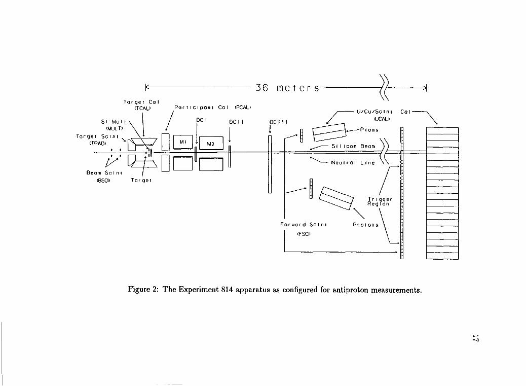
Figure 2: The Experiment 814 apparatus as configured for antiproton measurements.

Detector Abbreviationbeam telescope BSCItarget calorimeter T C A Ltarget paddles T P A Dmultiplicity array M U L Tparticipant calorimeter P C A Ltracking chambers D R C Hforward scintillators FSCIuranium calorimeter U C A L
Table 1: Detector abbreviations
19
all the detectors with associated four letter abbreviations. A list of the specific com
ponents such as electronic modules and photomultipliers used in each detector system
will be found in Appendix A.
The measurements to be discussed in this thesis were made using a 28Si beam
having a m o m e n t u m of 14.6 GeV/c per nucleon for a total m o m e n t u m of more than
400 GeV/c. Data were taken using three targets, Pb, Cu, and Al. Each target is
approximately 10% of a 28Si interaction length. Table 9 gives the exact dimensions of
the targets. The targets were chosen to be as thick as possible to maximize the number
of interactions without compromising the event characterization measurements. The
beam intensity used for these measurements was about 3 x 10⁵ particles per spill.

20
2 .2 .1 E n e r g y L o ss o f P a r t ic le s in M a t t e r
Detector response generally is determined by the way an incident particle loses energy
in the detector material. The dominant loss mechanism is from collisions of the
incident particle with atomic electrons in the absorbing medium. The average rate of
energy loss is described by the Bethe-Bloch formula:
V 2 m e72/?2iy \ 02d E Ar 2 2Z z 2~ Hi ~ a re m ec ~^~02 In (2.10)
Here,
N a : Avogadro’s number; 6.022 x 10²³ per mole
re: classical electron radius
m e: electron mass
z: charge of the incident particle
Z\ atomic number of the absorbing material
A: atomic weight of the absorbing material
/* v/c of the incident particle
T- i M - P2w ■vv max* m a x i m u m energy transfer for a single collision
/: ionization constant
6: correction for density effects.
Figure 3 shows a plot of Equation 2.10 for different projectiles incident on Pb. The
energy loss initially falls as l//?2, reaching a minimum when /3 & .96. The range of
energies for which d E / d x is near the minimum value is quite broad, covering most of
the region of interest for measurements of relativistic particles at the AGS. Particles
having an energy within this range are called m i n i m u m ionizing.

21
P(GeV/c)
Figure 3: The average energy loss (in units of M e V g _1c m 2) of particles in Pb as described by the Bethe-Bloch formula. Energy loss is plotted as a function of the m o m e n t u m of the incident particle.
The energy transfer to the electrons of the target atoms is a statistical process.
In some of the collisions a small amount of energy is transferred to the electrons in
the material. Such soft processes result in the excitation of the electrons to higher
atomic energy levels. More energetic hard collisions can cause ionization. If enough
energy is transferred to the electron during the reaction, the free electron can induce
ionization in subsequent collisions. These high energy ionizing electrons are called
6-rays or knock-on electrons.
2 .2 .2 B e a m D e fin it io n
The beam telescope (BSCI) serves the dual purpose of signaling the passage of a
silicon ion through the apparatus and providing the reference timing signal, or to, for
the experiment. Figure 4 shows a schematic picture of the system of beam defining

22
target
+---------- nbeam LJ
Figure 4: A schematic picture of the beam telescope consisting of the beam defining scintillators S2 and S 4, and the veto counters Si and S 3.
scintillators. A pair of thin plastic scintillator disks, S 2 and S 4, defines the beam
direction. A second pair of thick annular scintillators, Si and S 3, are used as vetoes
against off-axis beam particles. Table 2 gives the dimensions and distance from the
target of each of the elements of the beam telescope. The beam defining scintillators
are read out by two photomultiplier tubes each and the larger veto counters are
equipped with four photomultiplier tubes each. The photomultipliers for the second
of the beam defining scintillators, S 4, are chosen to have particularly good timing
properties as this scintillator provides the <0 for the experiment.
Pulse height information from all counters and the timing signal from S 4 are
available for use in the trigger logic. Signals from all counters are digitized and
recorded for use in the offline refinement of the beam definition.
2 .2 .3 S ig n a l P r o c e s s in g
The analog signals produced by a detector must be converted to an equivalent digital
form in order to be recorded by the data acquisition system. Signals carrying pulse
height information are digitized by analog-to-digital converters, or A D C ’s. These
devices are either charge sensitive, integrating the total signal current, or peak sensing,
S3

23
counter thickness inner diameter outer diameter distance from targetSi 0.4 1.5 15.0 652.8s 2 0.05 - 1.8 627.4s3 0.4 0.6 15.0 177.8s 4 0.05 - 0.9 203.2
Table 2: Dimensions and distances to the target for the elements of the beam telescope. All dimensions are in cm.
recording the m a x i m u m voltage of the signal. In the absence of a signal, the A D C
will record a pedestal value corresponding to a measurement of zero. As part of the
calibration process, the pedestal from each channel must be recorded and subsequently
subtracted from all measurements in that channel. Time signals are processed using a
time-to-digital converter (TDC). A scaler is used to count the number of oscillations
of an internal clock occurring between two signals. Alternatively, a T D C may consist
of a time-to-amplitude converter followed by an ADC.
2 . 3 D e t e c t o r s f o r E v e n t C h a r a c t e r i z a t i o n
2 .3 .1 T a r g e t C a lo r im e t e r
The target calorimeter (TCAL) provides a measurement of the energy produced trans
verse to the beam direction. This calorimeter is composed of 992 crystals of Sodium
Iodide doped with Thallium as the impurity activator. Nal(Tl) is an inorganic scintil
lator commonly used in nuclear and high energy applications for its good light output.
The crystals for this detector were originally elements of a pair of electromagnetic
calorimeters used by C E R N Experiment R807, the Axial Field Spectrometer. The
reconfiguration of the arrays as well as details about the testing, calibration, and

24
operation of the target calorimeter have been described extensively elsewhere[20].
The Nal(Tl) crystals are arranged in five walls surrounding the target assembly.
Four walls of crystals form an open-ended box with faces parallel to the beam axis.
The fifth array of crystals closes the upstream end of the box except for a hole through
which the beam passes. In order to measure correctly the transverse energy, it is
necessary to determine the angle at which the particle enters the detector. Arranging
the crystals in an approximately projective geometry with the long axis of each one
pointing at the target confines the energy deposition from a single particle to a few
crystals and makes the location of a crystal with respect to the target well defined in
angle.
Almost all the crystals are 13.8 c m in length, equivalent to 5.3 radiation lengths
and .33 hadronic interaction lengths. With this geometry, the pseudorapidity coverage
of the calorimeter side walls is — 0.5 < 77 < 0.8. For the back wall, the acceptance is
-2.5 < 77 < -1.2.
Signals from the detector elements are read out using vacuum photodiodes mounted
on the face of each crystal. After shaping, the signals are available for digitization
and recording by the data acquisition system.
The four side walls of the target calorimeter are lined with an array of 52 scintil
lator paddles (TPAD). Each paddle lies along a row of crystals parallel to the beam
axis. The paddles are coupled to photomultipliers through light guides. The output
signal from each photomultiplier is split. Part of the T P A D signal is s ummed and
discriminated to serve as a rough multiplicity measurement for trigger use. After
digitization, the remaining part of the split signal is recorded by the data acquisition
system.
25
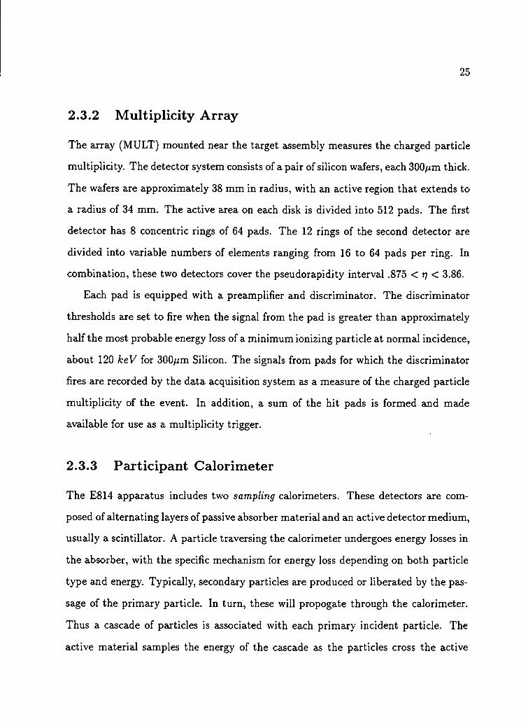
2 .3 .2 M u lt ip l ic i t y A r r a y
The array (MULT) mounted near the target assembly measures the charged particle
multiplicity. The detector system consists of a pair of silicon wafers, each 300/xm thick.
The wafers are approximately 38 m m in radius, with an active region that extends to
a radius of 34 m m . The active area on each disk is divided into 512 pads. The first
detector has 8 concentric rings of 64 pads. The 12 rings of the second detector are
divided into variable numbers of elements ranging from 16 to 64 pads per ring. In
combination, these two detectors cover the pseudorapidity interval .875 < tj < 3.86.
Each pad is equipped with a preamplifier and discriminator. The discriminator
thresholds are set to fire when the signal from the pad is greater than approximately
half the most probable energy loss of a minimum ionizing particle at normal incidence,
about 120 k e V for 300^zm Silicon. The signals from pads for which the discriminator
fires are recorded by the data acquisition system as a measure of the charged particle
multiplicity of the event. In addition, a sum of the hit pads is formed and made
available for use as a multiplicity trigger.
2 .3 .3 P a r t ic ip a n t C a lo r im e t e r
The E814 apparatus includes two sampling calorimeters. These detectors axe com
posed of alternating layers of passive absorber material and an active detector medium,
usually a scintillator. A particle traversing the calorimeter undergoes energy losses in
the absorber, with the specific mechanism for energy loss depending on both particle
type and energy. Typically, secondary particles are produced or liberated by the pas
sage of the primary particle. In turn, these will propogate through the calorimeter.
Thus a cascade of particles is associated with each primary incident particle. The
active material samples the energy of the cascade as the particles cross the active

26
layers. The participant calorimeter (PCAL) is a Pb/scintillator sampling calorime
ter designed to measure energy in the pseudorapidity range .83 < 77 < 3.9. The
calorimeter is made of four separate movable quadrants. This division allows the
beam aperture size to be varied by repositioning the quadrants. Each quadrant is
divided azimuthally into four triangular sections, each subtending 22.5°. These tri
angular sections are subdivided radially into eight sections for a total of 128 towers.
Layers of 1.0 c m thick lead absorber alternate with .03 c m scintillator plates to form
four separate depth segments. Every sixth absorber layer is made of iron for structural
support. T w o electromagnetic sections, each .4 interaction lengths (A) or 10 radiation
lengths, are followed by two hadronic sections of 1.6A each, for a total depth of 4A.
In order to transmit light from the scintillator layers to the photomultiplier tubes,
wavelength shifting fibers are bonded to the edges of the scintillator plates. Within a
tower, the fibers from each depth segment are bundled. Every fiber bundle is coupled
optically to a phototube with a polyurethane coupler and R T V disk. The signals
from the phototubes are digitized and are also available for use in the trigger.
2 . 4 F o r w a r d S p e c t r o m e t e r
2 .4 .1 T r a c k in g C h a m b e r s
The design of the E814 tracking chambers (DRCH) for the heavy ion environment
presented a particular challenge. The heavy ion beam passes directly through the
chamber so the detector must be protected against the propogation of 6-rays through
the detector. These high energy recoil electrons can produce many electron tracks
from secondary ionization in the chamber material, greatly increasing the difficulty
of pattern recognition. Since part of the experimental program involves the measure

27
ment of electromagnetic dissociation cross sections, it is necessary for the detectors
to be able to detect simultaneously both minimum ionizing particles and heavy ions.
Thus the chambers must have a large dynamic range. In addition, the detectors must
be able to handle large multiplicity events with a high local track density. As a final
requirement, the amount of detector material should be minimized to reduce multiple
scattering and hadronic interactions.
Three chambers form the D R C H system: DCI, DCII, and DCIII. The first of
these, DCI, is located between the two spectrometer magnets, D 8 and D9 (Figure 2).
DCI consists of a single wire plane above a cathode pad. DCII and DCIII, similar
in design and construction, have six drift planes apiece and one wire plane with a
cathode plane. The design and performance of the E814 tracking chambers has been
described in [21, 22, 23].
The three detectors were filled with a gas mixture of 50% argon-50% ethane at
atmospheric pressure. This gas mixture has a drift velocity of about 50/xro/ns at the
operating voltages of the chambers. In DCI, a slight amount of ethanol was added to
the gas as a quenching agent to reduce charge accumulation on the wires. This was
done by bubbling the gas through a bottle of ethanol maintained at a temperature of
0°C.
A typical drift chamber cell consists of an anode, or sense wire between two
cathode planes. Field-shaping wires on both sides of the anode wire provide a uniform
electric field through most of the drift region between the wires. The passage of
a charged particle through the chamber causes ionization in the detector gas. In
a uniform electric field the ionization electrons drift towards the anode wires at a
constant velocity. By measuring the time taken for the electrons to arrive at the
anode wire, the perpendicular distance of the trajectory of the charged particle from

28
the wire can be determined. Since only the absolute value of the distance from the
wire is measured, an ambiguity results as to whether the particle track passed to the
left or the right of the wire. This ambiguity is resolved during the pattern-recognition
process.
In order to measure the position of the particle in the direction parallel to the
wire, the last cathode plane of the chamber is divided into strips lying along the wire
direction. These strips are further divided into pads. The cloud of electrons on the
wire plane above this board causes a charge to be induced on the cathode plane. By
measuring the induced charge, the position of the charged particle along the wire can
be determined. Measuring the particle track in both x and y simplifies the problem
of track reconstruction considerably.
DCI is shown in Figure 5. The wire plane consists of 17 p m diameter gold-plated
tungsten anode wires alternating with stainless-steel field wires. The drift cell is
completed on the upstream side by an aluminized mylar window and downstream
by the cathode detector board, a three layer printed circuit board. The top layer of
the board is divided into pads connected by resistive strips. At intervals the pads
axe connected electrically to traces on the bottom layer of the board. These traces
lead to preamplifiers mounted on external circuit boards. The spacing between the
pads connected to the trace layer varies with the expected track density across the
board. In the region where the m a x i m u m number of tracks is expected, every fourth
pad is equipped with a preamplifier. In the medium density region every eighth pad,
and in the least densely populated region every tenth pad is connected to a trace.
The charge induced on the cathode plane will be shared among several of the pads
through the resistive strips. The position along the wire is determined as the centroid
of the induced charge distribution. The middle layer of the detector board is a ground

29
y— WINDOW ----------nELD WIRE
• ' --------- ANOOE WIRE PAD
v cuard strip
WMX3W
— CUARD STRFRcssnvc snap
Figure 5: The DCI pad chamber structure.
30
Pad Plane
O 0 O 0 O 0 O # O # O « O # O * O » O 0 O # O
• o * o * o # o * o * o * o * o * o * o » o *
O 0 O « O # O # O # O « O # O 0 O » O # O # O
• o # o * o # o * o * o * o « o * o * o * o *
O # O * O # O 0 O # O * O # O # O # O * O # O
• O 0 O 0 O 0 O 0 O # O 0 O # O # O # O 0 O «
O # O 0 O « O # O # O 0 O 0 O # O # O # O # O
• Anode Wires Cathode Planes
O Field Wires
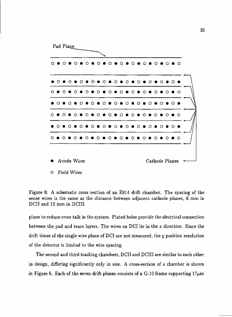
Figure 6: A schematic cross section of an E814 drift chamber. The spacing of the sense wires is the same as the distance between adjacent cathode planes, 6 m m in DCII and 12 m m in DCIII.
plane to reduce cross talk in the system. Plated holes provide the electrical connection
between the pad and trace layers. The wires on DCI lie in the x direction. Since the
drift times of the single wire plane of DCI are not measured, the y position resolution
of the detector is limited to the wire spacing.
The second and third tracking chambers, DCII and DCIII are similar to each other
in design, differing significantly only in size. A cross-section of a chamber is shown
in Figure 6. Each of the seven drift planes consists of a G-10 frame supporting 17/zm

31
Figure 7: The chevron pad structure for DCII and DCIII.
gold-plated tungsten anode wires and stainless-steel field wires. The wire planes are
separated by aluminized mylar cathodes. In order to facilitate the pattern recognition
process, the positions of the field and sense wires are staggered on alternate planes.
The wires in DCII and DCIII lie parallel to the y-axis, giving the best position
resolution in the bend plane of the spectrometer.
The final cathode plane is a segmented detector board that allows position mea
surement in the direction along the wires, as in DCI. However, for DCII and DCIII
the charge division is geometric rather than resistive. The pads on the top layer of
the detector board are chevron shaped, as in Figure 7. By measuring the relative
amounts of induced charge shared by neighboring pads along a wire, a reasonable
determination of the position of the charged particle trajectory along the wire can be

32
zero-crossing
discriminator
T D C
Figure 8: A block diagram of the electronics chain for a single channel of a drift plane.
made. The resolution thus obtained is better than 10% of the distance between the
points at which the charge is measured. Like DCI, the detector board is divided into
regions of three different pad densities with the size of the chevrons varying across
the detector board according to the expected particle density In the region of lowest
density the pads below neighboring pairs of wires are electrically coupled.
The choice of very thin anode wires allows saturation of the avalanche gain as the
primary ionization increases. This reduces the relative size of the 28Si signal by a
factor of 3.3. Since the primary ionization increases with projectile charge Z as Z 2,
without this saturation effete the anode signal from a 28Si ion would be almost 200
times larger than that for a minimum-ionizing particle.
Tracking Chamber Electronics
The electronics chain for the drift sections is shown in Figure 8. Each sense wire is
equipped with a low noise common-base preamplifier mounted outside the chamber.
The preamplifier output passes through a unipolar shaping amplifier having a 12 ns
lower threshold. discriminator
33
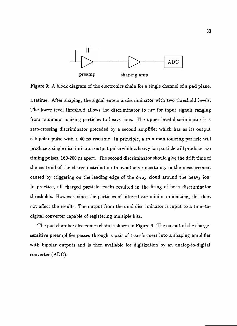
preamp shaping a m p
Figure 9: A block diagram of the electronics chain for a single channel of a pad plane.
risetime. After shaping, the signal enters a discriminator with two threshold levels.
The lower level threshold allows the discriminator to fire for input signals ranging
from minimum ionizing particles to heavy ions. The upper level discriminator is a
zero-crossing discriminator preceded by a second amplifier which has as its output
a bipolar pulse with a 40 ns risetime. In principle, a minimun ionizing particle will
produce a single discriminator output pulse while a heavy ion particle will produce two
timing pulses, 160-200 ns apart. The second discriminator should give the drift time of
the centroid of the charge distribution to avoid any uncertainty in the measurement
caused by triggering on the leading edge of the <S-ray cloud around the heavy ion.
In practice, all charged particle tracks resulted in the firing of both discriminator
thresholds. However, since the particles of interest are minimum ionizing, this does
not affect the results. The output from the dual discriminator is input to a time-to-
digital converter capable of registering multiple hits.
The pad chamber electronics chain is shown in Figure 9. The output of the charge-
sensitive preamplifier passes through a pair of transformers into a shaping amplifier
with bipolar outputs and is then available for digitization by an analog-to-digital
converter (ADC).

34
photomultiplier ■light guide
120 c m scintillator
10 cm
Figure 10: Forward scintillator slat
2 .4 .2 S c in t i l la to r H o d o s c o p e
The scintillator hodoscope (FSCI) is used to measure the flight time of charged par
ticles through the forward spectrometer. This measurement, together with the m o
mentum measurement from the tracking chambers, provides particle identification.
The FSCI also allows simultaneous measurement of the charge of the particle and the
x and y coordinates of the particle track through the hodoscope.
The FSCI system consists of three separate walls, each located approximately 5
meters upstream from a calorimeter section. The largest and farthest downstream of
these walls, located 31.3 m from the target, is made of 44 slats of plastic scintillator.
For the antiproton measurements, only this back wall is used. Each scintillator slat
is 120 c m long, 10 c m wide, and 1 c m thick.

35
to D A Q
to D A Q
to trigger and D A Q
dynode 1
dynode 2 sum F E R A to trigger and D A Q
Figure 11: The signal path of the photomultiplier output from a forward scintillator slat. The analog sum includes the top and bottom photomultipliers
A typical scintillator is shown in Figure 10. Both ends of the slat are optically
coupled to photomultiplier tubes through light guides.
Figure 11 shows the forward scintillator signal path. Signals from the photomul
tiplier anodes are split; one output is sent to an A D C and recorded for the charge
measurement and the other is discriminated by a Philips 7106 dual output discrimina
tor. The two discriminator signals are used for the timing measurement. One of the
signals is digitized by a T D C and recorded; the other is digitized by a Fast Encoding
Readout T D C (FERET) and is available for use by the trigger system. The dynode
signal is digitized using a Fast Encoding Readout A D C (FERA) and is also sent to
the trigger system.
2 .4 .3 U r a n iu m C a lo r im e t e r
The final detector in the forward spectrometer is the uranium/copper/scintillator
sampling calorimeter (UCAL). This detector allows an additional check on the iden
tification of a particle passing through the spectrometer. In addition to the energy

36
Figure 12: The anode signal path of the photomultiplier output for the uranium calorimeter. The analog sum is over all 24 signals in a stack.
measurement, the calorimeter is designed to provide a measurement of the x and y
position of incident particles.
The three sections of the U C A L are shown in Figure 2. As with the forward
scintillator, only the large downstream wall is used in these measurements. The
forward calorimeter wall is made of 20 individual stacks 120 c m high, 20 c m wide,
and 75 c m deep. A stack is composed of 41 depth units with each unit consisting
of one layer of 5 m m thick copper and two layers of 3 m m thick depleted uranium
as absorber materials. The absorber layers alternate with sheets of 2.5 m m thick
plastic scintillator. These scintillator sheets are divided vertically into 12 optically
decoupled towers. A bar of wavelength shifter is mounted along either side of each
tower. These bars, which extend from the front to the rear of the tower, provide the
optical coupling from the scintillator layers to photomultiplier tubes located at the
back of eack stack. Each wavelength shifter is equipped with one photomultiplier for
a total of 24 tubes per stack.
The photomultiplier anode signal path is shown in Figure 12. After being split,
part of the signal is digitized by an A D C and recorded. An analog sum of the output
from all 24 photomultipliers in a given stack is also formed. This summed signal
is split and used as inputs both to a discriminator and a FERA. The discriminator
37
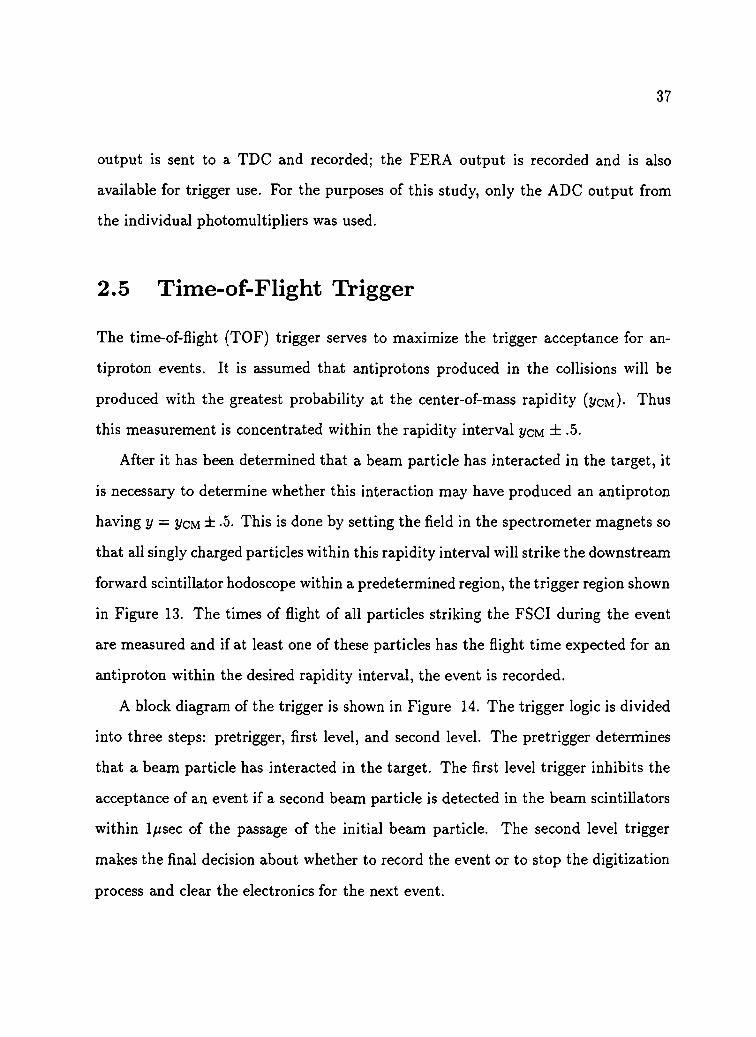
output is sent to a T D C and recorded; the F E R A output is recorded and is also
available for trigger use. For the purposes of this study, only the A D C output from
the individual photomultipliers was used.
2 . 5 T i m e - o f - F l i g h t T r i g g e r
The time-of-flight (TOF) trigger serves to maximize the trigger acceptance for an-
tiproton events. It is assumed that antiprotons produced in the collisions will be
produced with the greatest probability at the center-of-mass rapidity (j/c m )- Thus
this measurement is concentrated within the rapidity interval j/c m ± -5.
After it has been determined that a beam particle has interacted in the target, it
is necessary to determine whether this interaction may have produced an antiproton
having y = j/cm ± -5. This is done by setting the field in the spectrometer magnets so
that all singly charged particles within this rapidity interval will strike the downstream
forward scintillator hodoscope within a predetermined region, the trigger region shown
in Figure 13. The times of flight of all particles striking the FSCI during the event
are measured and if at least one of these particles has the flight time expected for an
antiproton within the desired rapidity interval, the event is recorded.
A block diagram of the trigger is shown in Figure 14. The trigger logic is divided
into three steps: pretrigger, first level, and second level. The pretrigger determines
that a beam particle has interacted in the target. The first level trigger inhibits the
acceptance of an event if a second beam particle is detected in the beam scintillators
within 1/zsec of the passage of the initial beam particle. The second level trigger
makes the final decision about whether to record the event or to stop the digitization
process and clear the electronics for the next event.

38
Figure 13: The active scintillator region for the time-of-flight trigger.
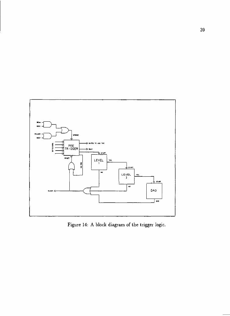
Figure 14: A block diagram of the trigger logic.

40
The first requirement of the pretrigger is that the beam trigger condition is sat
isfied. The pulse height in each of the beam defining scintillators must be consistent
with the passage of a particle having a charge Z = 14. In addition, the signal from
both of the veto scintillators must be below that expected for a minimum ionizing
particle. The logic required to satisfy the beam trigger is thus:
B = Si • S2 • S 3 ' S 4 • busy
where the busy signal is generated once the pretrigger is satisfied. This ensures that
a beam trigger is only satisfied when the system is free to process the event.
The final requirement for the pretrigger is that a nuclear interaction has occurred.
In order to satisfy this requirement, information from several of the detectors associ
ated with the target are used. The logic to satisfy the interaction condition is:
INT = ( T P A D • M U L T + P C A L • M U L T ) ■ B
where T P A D and M U L T indicate that the numbers of particles striking the target
paddles and multiplicity array exceed 5 and 25, respectively. The P C A L requirement
is that a minimum of 5 G e V of energy is detected in the participant calorimeter. The
thresholds were adjusted so that approximately 10% of the events which satisfy the
beam requirement also satisfy the pretrigger when the Cu target is in place. This
indicates that the pretrigger requirement reflects the 0.1 A target.
If the pretrigger requirement is satisfied, a gate is generated to strobe the A D C ’s
and to stop or start the T D C ’s, depending on the operating mode. In addition, the
Level 1 trigger begins. If the beam scintillators do not indicate a second beam particle
within lfisec of the trigger particle, the Level 1 trigger is satisfied and the Level 2
trigger is started.

41
Figure 15: A block diagram of the second level trigger. Each F E R A processes 16 channels.
Trigger Level 2 accepts as input the discriminated timing signal from each FSCI
photomultiplier, top and bottom, as well as the amplitude pulse from the dynode
sums. Initially, the gains of the photomultipliers are equalized using a 106R u source
to allow the use of a global set of slewing constants. The amplitude information is used
to determine an online slewing correction for the time-of-flight measurement. This
slewing correction adjusts the timing signal to remove the pulse height dependence
from the timing, allowing for an average online timing resolution of 600 ps. Each
signal has a value corresponding to zero time, to, subtracted to correct for differences
in flight path and cable delays.
Figure 15 is a diagram of the second level trigger. The F E R E T - F E R A combination
acts as a two step time-to-digital converter which processes the discriminated signal
from each photomultiplier on the forward scintillator trigger region (see Figure 11).
The F E R E T measures the time elapsed between the beam trigger and the output pulse

42
from the discriminator. The FERA, gated by the pretrigger signal, generates a signal
with amplitude proportional to this elapsed time. This signal, with to subtracted, is
input into the first arithmetic logic unit, A L U 1, and a switch module which controls
the signal processing. A L U 1 computes the time difference, At = tx — t2 between
the top and bottom photomultipliers. The digitized dynode outputs and 8t are used
as inputs to the first memory lookup unit ( M L U 1) to access the stored slewing
corrections.
The output of M L U 1 is the slewing correction, St. The values for fy, t2, and St are
input into A L U 2 which computes t\ + t2 — St, the value of which is proportional to the
average time-of-flight as measured by the top and bottom photomultipliers. These
values are monitored by the data stack, a passive device which allows the slewing
corrected times to be recorded by the DAQ. They are also input to M L U 2 which
determines whether the times are later then a preset value. If one of the time values
exceeds this limit within a set interval, the level 2 trigger is satisfied and the event is
recorded. Most of the data were taken with the timing limit set such that particles
arriving at the hodoscope between 3 ns and 30 ns later that a v = c particle were
accepted. About one-fifth of the data were taken with the lower limit of the timing
window at 2 ns to ensure good acceptance for kaons to be used for confirmation of
particle identification.
2 . 6 D a t a A c q u i s i t i o n S y s t e m
Processing of the signals from the various detectors is done using a combination of
Fastbus and C A M A C electronics. The C A M A C standard is used for the trigger logic
and the electronics for the the FSCI and M U L T detectors. Digitization of signals from

43
other detectors is done using the Fastbus system. Figure 16 shows a schematic picture
of the E814 data acquisition system and digitization electronics. Each Fastbus crate
is controlled by a S L A C Scanner-Processor (SSP). Signal flow and event management
is performed by an SSP located in the master Fastbus crate. This crate contains
the Computer Fastbus Interface (CFI) linking the master crate to the main data
acquisition computer, a Microvax III. The master crate also contains a 4 Mbyte
memory module used as a data buffer and a Struck Fastbus Branch Driver (FBD)
which provides the connection to the C A M A C branch highway. W h e n the system
receives a signal from the second level trigger indicating a good event, the master
SSP generates a busy signal to inhibit subsequent triggers until the event handling
is complete. A signal is also sent to the signal processors in the lower level Fastbus
crates to initiate reading of the modules in the crates. The master SSP then builds
the event from the data from the C A M A C branch and from the lower level Fastbus
crates. The event is written into the memory module and the busy signal is cleared
to free the system for the next trigger. At the end of the A G S beam spill, the data is
transferred from the memory module to the Microvax III. The data is recorded using
one of two available high-speed 9 track tape drives. The Fermilab software package
VAXONLINE [24] provides the user interface to control the data acquisition system. The
VAXONLINE program also provides a pool of events for online monitoring of detector
performance.
2 . 7 A c c e p t a n c e
The acceptance for the antiproton run was determined using a Monte Carlo simulation
of the complete E814 apparatus. The C E R N computer library program GEANT [25]

44
ADC
ADC
ADC
SSP
TDC
Lower level Fastbus crates
C A M A C Branch
FBD
CFI
4Mb
SSP
Master Fastbus Crate
to tape drives
Figure 16: A block diagram of the data acquisition system.

45
was used as the basis for the development of the Monte Carlo program. The GEANT
library provides a framework for establishing the detector geometry and for simulating
the physical processes describing the interaction of particles in the detector materials.
A sample of antiprotons was generated with a uniform distribution in pt and
y. The generated events were propagated through the apparatus and the time of
flight and position at the scintillator hodoscope were determined. Those antiprotons
striking the trigger region of the hodoscope with a time of flight greater than 3 ns
relative to a particle having v = c were accepted. Figure 17 shows the distribution in
pt and y of the accepted events for 30000 Monte Carlo events.
The acceptance of the E814 apparatus for antiprotons run is dominated by two
effects. First, the time-of-flight trigger sharply limits the acceptance at high rapidity.
Second, the small aperture in the P C A L makes the p t acceptance strongly rapidity
dependent. Thus, the shape of the pr integrated rapidity spectra reflect the natural
rapidity distribution convolved with the the increased p t acceptance at higher rapidi
ties. The geometrical acceptance is complicated further by the fact that the P C A L
opening is rectangular, leading to acceptance losses which depend on the orientation
of the particle within this opening. Since the GEANT simulation includes the interac
tion of the antiprotons traversing the spectrometer material, annihilation and losses
from other interactions are included. The results from the simulation are used to
correct for these effects (see Section 5.3).
Given the limited angular acceptance of the spectrometer, only a small number of
the antiprotons produced will be detected. In order to estimate the total experimental
acceptance for antiprotons, a second ensemble of antiprotons is generated as input
to the GEANT simulation of the E814 apparatus. The antiprotons are assumed to be
produced with a Gaussian rapidity distribution having a width of 0.5 and a mean

Tran
sver
se
mom
entu
m
(GeV
/c)
46
Figure 17: Accepted antiprotons as a function of transverse m o m e n t u m and rapidity for Monte Carlo generated events distributed uniformly in pt and y.

47
value of 1.7 units of rapidity. Using the result of Brookhaven Experiment 802, the
antiprotons are assumed to have a pt distribution
^ = pt exp - + - m p) /&, (2.1 1)
where b = 0.141 GeV/c. Figures 18 and 19 show the rapidity and transverse m o
mentum spectra for both the generated and the accepted events. Of the 100000
antiprotons produced, 402 pass through the P C A L opening and satisfy the time-of-
flight trigger. Thus, the total acceptance for antiprotons is found to be 0.4%. Of
course, deviations of the real antiproton distribution from that assumed above may
make the actual acceptance different from this value.

48
Ropidity Rapidity
Rapidity
Figure 18: (a) Generated antiproton rapidity distribution, (b) Accepted antiproton rapidity distribution, (c) Fraction of antiprotons accepted.

49
„ 20000 1000
p, (G e V /c )
T5VQ .V U u o in c o
1
0.8
0.6
0.4
0.25 0.5 0.75 1 1.25 1.5
p, (G e V /c )
(c)
1.75
Figure 19: (a) Generated antiproton pt distribution, (b) Accepted antiproton distribution, (c) Fraction of antiprotons accepted.

C h a p t e r 3
T r a c k i n g a n d P a t t e r n r e c o g n i t i o n
The forward spectrometer, consisting of tracking chambers, scintillators, and calorime
ters, provides information for particle indentification and measurement of kinematic
quantities. After calibration, the data for an event consists of signals from each of
the detectors: drift times for individual wires in the drift chambers, deposited charge
for the pad plane channels, time and pulse heights for both phototubes on each scin
tillator slat, and the energy measured in each calorimeter tower. The purpose of the
pattern recognition program is to correlate the signals which mark the passage of
each particle through the spectrometer. Once this has been done, the momentum,
velocity, and energy of the particle are determined.
3 . 1 Q U A N A H
The pattern recognition code for the forward spectrometer, named QUANAH after an
Indian tracker named Quanah Parker, was developed at Yale. In order to simplify
the following discussion, it is useful to define a few terms:
50

51
clusters and elements The position at which a particle strikes a detector is stored
in an array, termed either a cluster array, if the elements of the array have
position information, or an element array if the elements have both position
and directional information. Any associated information, such as charge, energy,
and time of flight, is also stored in the array.
segment A grouping of clusters and elements lying along a straight line downstream
of the spectrometer magnet.
candidate A segment whose projection back through the magnet is consistent with
the trajectory of a charged particle originating at the target. In addition to the
segment, the candidate may also have an associated cluster from DCI.
track Unique candidates are stored as tracks. If more than one candidate shares the
same segment, the candidates are tested to determine which is most likely to
represent the true path of the particle.
3 . 2 U n c e r t a i n t i e s
In order to assure a high efficiency in the full pattern recognition process, it is neces
sary to make individual comparisons of measurements between detectors as efficient
as possible.
To accomplish this, all measurements which have approximately gaussian reso
lutions are required to agree within 3<r. Those detectors with resolutions which are
non-gaussian, such as the x position of a scintillator hit which is know only to the
width of the slat, are required to agree within one half-width of the detector.

52
Figure 20: Q U A N A H coordinate system
3 . 3 S e g m e n t a n d C l u s t e r F o r m a t i o n
The coordinate system used in the following discussion is shown in Figure 20. The
origin of the system is at the position of the target. The beam direction defines the
positive z-axis and the positive y direction is taken to be vertically upwards. The
positive x-axis is chosen to form a right-handed coordinate system.

53
3 .3 .1 P a d C h a m b e r C lu s t e r s
The data from the pad chambers are measurements of the image charge induced
on each pad by electrons drifting to the plane of wires above the pad plane after
the passage of a charged particle through the chamber gas. These charges must
be converted into position information by employing an appropriate charge division
scheme. The calibrated data is stored in an array indexed by A D C channel. Since
the geometry of the detector board is irregular and the order of channel readout is
dictated by the necessity to compact the traces as much as possible, the indexing of
the data array is not directly useful for determining the placement of clusters. For
simplicity in using the pad detectors, a coordinate system is established which assigns
three indices of an array to each pad. The first two are indices following the x and
y spatial coordinates; the origin of this local system is the lower right corner of the
board when looking at the detector from the beam direction. The third index gives
the density of the region, with a density of 1 being the coarsest and a density of 3
corresponding to the region of fine segmentation in the center of the board.
Since each A D C channel is read out for every event, it is first necessary to deter
mine which pads have induced charge. This is done in two steps. First, the A D C
values for all pads lying beneath a given pair of wires are summed. The sums in
DCII and DCIII are made by wire pairs to avoid redundancy when considering the
coupled pads. Thus there are half as many unique wire sums as there are sense wires
in the wire plane. Each wire sum is tested against a threshold and those wires which
show a combined charge above the threshold are flagged. Individual channels along a
flagged wire are then tested against a single channel threshold and the channel n u m
bers corresponding to pads with charge above this threshold are stored in an array of
hits.

54
Once the bank of pad hits is formed, the cluster formation proceeds. The axray is
searched to determine the largest charge deposit, and this channel forms the center of
the first cluster. A table containing the location and number of neighboring channels
is consulted to complete the cluster. While this table can be readily changed to
accomodate various charge-sharing schemes, for the purposes of this analysis the
neighboring pads are taken to be those immediately adjacent to the central pad along
the wire direction. No charge sharing across wires is considered. A n additional table
containing the location in x and y of the pads in the cluster is consulted. The position
of the cluster center along the wire direction is determined to be the average of the
positions of the pads in the cluster with each pad position weighted by the A D C value
for that pad. For DCII and DCIII, this position is:
_ J/t<7t + V c Q c + V b Q b to-,1/CLUSTER — ;---- ;------9t + 9c + 9b
and for DCI:
_ x lQl + XcQc + xRqR /o io\^cluster — ------ ;---- ;------ 10.io)9l + 9c + 9r
where yc(zc) is the position of the central pad, yT(xL) and yB(xR) are the positions
of the adjacent pads, and qc, 9t(9l)> and 9b(9r) are the measured charges. In the
dimension perpendicular to the wires, the position is taken to be the wire location
for the single pads, or halfway between the two wires for the ganged pads.
All pads used in the cluster formation are subsequently removed from the hit
bank, and the process is repeated. W h e n two clusters overlap, this procedure tends
to shift the cluster positions towards the cluster with the lower total charge deposit.
However, the low multiplicities in the region of interest make this effect negligible for
the analysis of this data. In addition to the location of the cluster center, the total
charge of the cluster is stored in the cluster arrays for the pad chambers.

55
All pattern recognition algorithms were designed to work with the m a x i m u m ef
ficiency by finding all possible solutions. In some cases this leads to the introduction
of extraneous solutions. In the cluster-finding algorithm, these ambiguities are gener
ally caused by either charge-sharing across wires or by capacitive pickup on the larger
pads. For the pads, the resolution of the wire planes in the x direction is sufficient to
assure the correct association of clusters and elements when extraneous solutions lie
on adjacent wires. The noise clusters are not generally associated with elements and
do not pose a problem since they lie in a region of the chamber where the particle
multiplicities are low.
3 .3 .2 D r i f t C h a m b e r E le m e n t s
The calibrated data from the drift planes are stored as an array of hits containing the
measured distances from the sense wires. As with the pad planes, these positions are
given with respect to a local coordinate system, with the origin of the system being
the first sense wire on the second plane of each detector. Since all wires run parallel to
the y-axis, the drift planes give positions only in the x direction. At this level of the
analysis, each firing of the wire has two associated hits since the left-right ambiguity
(see section 2.4.1) has not yet been resolved. In addition, the plane number (1-6) is
stored in the hit array.
Track elements are found using a depth-first, or ’’tree” algorithm. Links are formed
between each hit position on a plane and the hits on the next plane. Then beginning
from a hit position on the first plane, each possible path of links is followed. After
each step, the slope of the connecting link is found. A particular path is rejected if
the change in slope from one step to the next exceeds a fixed value. All acceptable
paths are stored as possible elements and the hits (and the accompanying left-right

56
ambiguity points) are removed from further consideration.
In order to overcome detector inefficiencies, the algorithm allows the formation
of elements having fewer than six hits. After all possible six-hit elements have been
found, all five-hit elements, four-hit, and then three-hit elements are formed. W h e n
the formation of all potential elements is complete, there may be many elements which
share wire hits. These have been termed brothers, and it is necessary to choose the
brother which most probably reflects the correct path for the charged particle through
the chamber. In order to perform this brother elimination, a linear least-squares fit
through all the points of each brother is found, and the one with the smallest x 2 is
chosen as the correct element.
3.3.3 Scintillator H o d o s c o p e Clusters
Calibrated data from the A D C ’s and T D C ’s which process the signals from the scin
tillator hodoscope are stored in arrays indexed by slat number. The x position at
which a charged particle strikes the hodoscope is known to within the width of one
scintillator slat, 10.16 cm. It is possible to determine the y position by comparing
the times that it takes the light to travel along the scintillator to the phototubes at
opposite ends. Thus the y position is
vV — ^ t o p ^bottom)
where v is the velocity of light in the scintillator and ttop and bottom are the slewing-
corrected T D C values for the top and bottom phototubes respectively. In addition to
storing the x and y coordinates, the scintillator cluster array also contains the charge
and time-of-flight of the particle as measured by the hodoscope.

57
3.3.4 U r a n i u m C a l o r i m e t e r Clusters
Using a cluster-finding algorithm developed for the Uranium Calorimeters, it is gener
ally possible to determine the position and energy of particles impacting the calorime
ter wall. For the purposes of the antiproton analysis, the calorimeters could not be
used in this mode because the threshold for cluster formation could not be set low
enough to have complete efficiency for the lowest m o m e n t u m antiprotons. The ex
pected total energy deposited in the calorimeter by an antiproton of m o m e n t u m p
is
•^deposited = Fkinetic "t" 2lTlp (3.15)
where Fkinetic = yfp2 + m ^ — nip. For an antiproton having a m o m e n t u m of 1.4 GeV/c,
the lowest value of interest in this study, the expected energy deposited is 3.6 GeV.
The fraction of the total energy contained in the peak tower is a function of the
position within the tower at which the energy is deposited. The minimum energy
deposited in the peak tower is about 40 % of the total cluster energy. Thus the
threshold for efficient cluster-finding must be set below 1.4 GeV. W h e n the threshold
is set below this value, false clusters are formed where the pedestal for a tower is
particularly high. W h e n these false clusters are formed near real clusters, the clusters
are often incorrectly flagged as contaminated.
Instead of using the Uranium Calorimeter clusters as an integral part of the pattern
recognition, the clusters were formed using the SCAVENGER program. The rest of the
track is formed, as described below, and projected onto the face of the calorimeter.
The peak tower is taken to be the one indicated by this projection. Tower energies
axe summed over an area 4 towers vertically and 3 towers horiziontally centered on
the peak tower.
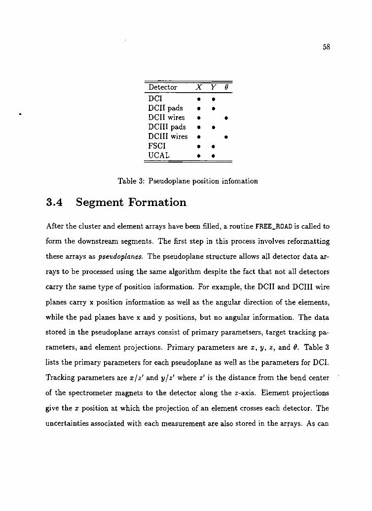
58
Detector X Y 6
DCI • •
DCII pads • •DCII wires • •
DCIII pads • •DCIII wires • •FSCI • •U C A L • •
Table 3: Pseudoplane position infomation
3 . 4 S e g m e n t F o r m a t i o n
After the cluster and element arrays have been filled, a routine FREE_R0AD is called to
form the downstream segments. The first step in this process involves reformatting
these arrays as pseudoplanes. The pseudoplane structure allows all detector data ar
rays to be processed using the same algorithm despite the fact that not all detectors
carry the same type of position information. For example, the DCII and DCIII wire
planes carry x position information as well as the angular direction of the elements,
while the pad planes have x and y positions, but no angular information. The data
stored in the pseudoplane arrays consist of primary parametsers, target tracking pa
rameters, and element projections. Primary parameters are i, y, z, and 6. Table 3
lists the primary parameters for each pseudoplane as well as the parameters for DCI.
Tracking parameters are xjz' and yjz1 where z' is the distance from the bend center
of the spectrometer magnets to the detector along the 2-axis. Element projections
give the x position at which the projection of an element crosses each detector. The
uncertainties associated with each measurement are also stored in the arrays. As can

59
be seen from Table 3, no pseudoplane contains a complete set of measurements. Miss
ing information is flagged by giving a negative value to the associated uncertainty.
The tree algorithm is used as in the wire routine to form links and to climb the links
in order to form the segments. The clusters and elements within the pseudoplane
array are referred to as sub-segments.
In order to compare the sub-segments, the procedure is somewhat more compli
cated than in the case of the wire planes, which involve measurements of single points
along one axis. The segments formed must be consistent with the track of a particle
which has passed through the opening in the P C A L after being created at the target.
A n additional complication is that the sub-segments must match in x, y, and 6. These
requirements are met by checking two different criteria for consistency. The first is
the requirement that the sub-segments be trackable\ this requirement establishes that
the link between the sub-segments could have come from the target. Checking the
tracking in the y direction is simple since the expected trajectory from the target is
a straight line. Measurements oiyjz must agree within measurement uncertainties.
The consistency check for measurements along the x-axis is more complicated since
the x-z plane is the bend plane of the spectrometer. To simplify the algorithm, the
pair of spectrometer magnets is described using a single-bend model and small-angle
approximations are used. For fixed x on a detector located at z', real tracks through
this point will have an average slope value of x/z'. The hole in the participant
calorimeter fixes the range of acceptable slopes within a cone of half-angle Do/ z',
where D 0 is determined by the size of the P C A L opening. Thus, the comparison
between sub-segments to ensure that the pair is trackable back to the target within
error is:
I x 2/z2 - x xfz\ |< Do I l/z[ - l/z '2 I -(-^(Xi/zi) + 5{x2/z2). (3.16)

60
The tracking parameter T is T R U E if the subsegments satisfy Equation 3.16. Since
the dispersion matrix D o | 1 /zj — l/z2 | can be computed in advance, the comparison
becomes both simple and efficient.
In order to satisfy the requirement of pointing between two sub-segments, the
measurements of each of the two detectors being compared must point at each other.
This is determined by checking that the projection of each measurement onto the other
agrees within uncertainties. Those measurements which do not carry the angular
information needed to form a projection are assigned a value of TRUE for the individual
pseudoplane pointing parameters Pi. The complete pointing requirement P is then
P = P!.AND.P2.
Consideration of both tracking and pointing allows some choice in the logic used
for segment formation. For the purposes of this analysis, the m a x i m u m efficiency
is gained by allowing segments to be formed which pass either the tracking or the
pointing requirement. Thus the final logic test for formation of a segment is
T.0R.(Pi.AND.P2).
After the segment has been formed, a linear fit is made to both x and y measure
ments. The angles the segments forms in the x — z plane and the y — z plane are
computed as 6 and <f> respectively.
3 . 5 C a n d i d a t e F o r m a t i o n
Once the measurements downstream of the magnets have been linked together as
possibly having an origin at the target, the routine MAGNATRACK performs the tracking
through the magnetic field, matches the segments with clusters in DCI, and computes

61
the magnetic rigidity 31 as well as the spatial coordinates x and y and the angles 0 and
4>. Track parameters determined at the target axe given a subscript 0; measurements
at DCI, DCII, and DCIII are given a subscript of 1, 2, and 3 respectively. All track
comparisons are performed assuming a model of circular tracks through the magnets.
As an initial step, a loop is made through all segments found by FREE.ROAD. Each
segment is projected back through the magnetic field and a first estimate of 60, xo,
1R are made. From this estimate, the x-position of the candidate track at DCI is
calculated. The array of DCI clusters is checked to determine whether any of the
clusters match the estimated position within measurement uncertainty. The pair
may be checked for agreement in x and y, or for the x value alone. If a compatible
cluster is found, the segment-cluster pair is stored. If no acceptable match is found,
the candidate is flagged as having incomplete information.
The final step is to recalculate the output values. The Newton-Raphson method
is used to determine the final value of From this angle, 31 is determined. Final
values for $o, <j>o, x 0, and yo are calculated and stored in the candidate array.
3 . 6 T r a c k F o r m a t i o n
Since the pattern recognition algorithms are designed to find all possible solutions,
some extraneous solutions will be introduced. This generally happens when two tracks
are closely spaced and the clusters or elements are not uniquely associated with one
acceptable track candidate. As a final step in the pattern recognition process, it
is necessary to eliminate the extraneous solutions, termed cousins. The subroutine
FREDDY.KRUGER is used to eliminate the cousins, leaving a unique track for each set
of clusters and elements.
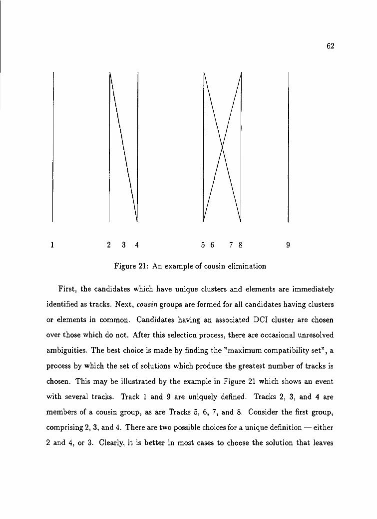
62
3 4 5 6 7 8
Figure 21: An example of cousin elimination
First, the candidates which have unique clusters and elements are immediately
identified as tracks. Next, cousin groups are formed for all candidates having clusters
or elements in common. Candidates having an associated DCI cluster are chosen
over those which do not. After this selection process, there are occasional unresolved
ambiguities. The best choice is made by finding the ’’m a x i m u m compatibility set”, a
process by which the set of solutions which produce the greatest number of tracks is
chosen. This m a y be illustrated by the example in Figure 21 which shows an event
with several tracks. Track 1 and 9 are uniquely defined. Tracks 2, 3, and 4 are
members of a cousin group, as are Tracks 5, 6, 7, and 8. Consider the first group,
comprising 2, 3, and 4. There are two possible choices for a unique definition — either
2 and 4, or 3. Clearly, it is better in most cases to choose the solution that leaves

63
two tracks rather than one. The second group, 5-8, has two solutions, each with two
tracks. In such a case where the set of m a x i m u m compatibles is still not unique, the
final selection is made by examining a quality factor for the candidates. The quality
factor is formed by determining the average number of standard deviations by which
the fitted track missed the measured values. This quality factor ranges from 0 for a
perfect track, to 3 which indicates that the track was off by 3a for every measurement.
The candidate with the smallest quality factor is chosen and the track array is filled
with all quantities and associated uncertainties necessary for subsequent analysis as
well as array indices which allow references back to the candidate, segment, cluster
and element arrays, and the original data arrays.

C h a p t e r 4
S p e c t r o m e t e r R e s o l u t i o n s a n d
E f f i c i e n c i e s
The capability for particle identification provided by the forward spectrometer makes
it possible to measure production cross sections for various particle species. Thus, it
is necessary to understand the efficiency with which each detector operates within the
system so that the probability to observe a particle passing through the spectrome
ter is known. Each detector and its associated chain of electronics has an intrinsic
inefficiency. Some inefficiencies will also arise in the comparison of measurements
from the different elements of the spectrometer. Careful measurements of the de
tector resolutions provide essential information to allow m a x i m u m efficiency for the
pattern-recognition process and to determine the effect of the final analysis cuts. In
this chapter, the methods used to evaluate these resolutions as well as the effectiveness
of each detector as a part of the spectrometer are discussed, and the total detection
efficiency is found.
64

65
4 . 1 P a d D e t e c t o r R e s o l u t i o n s a n d E f f i c i e n c i e s
The efficiencies of the pad detectors were evaluated using a data sample taken from
the study of central collisions. In this configuration, the spectrometer was tuned to
accept positively charged particles and the trigger selection was made on events from
central collisions. A n offline selection was made on the resulting events, requiring
that all events used had one and only one track element formed in DCIII. In this way,
a sample was formed which consisted predominantly of events with a single proton
track. It is important to note that no requirement of tracking through the entire
system was used in the sample selection. Thus there was no bias towards tracked
events. The element requirement in DCIII was used simply to eliminate most of the
events in which noise or delta rays might lead to the formation of false track segments.
The effective y resolutions of the cathode pads for the drift chambers were mea
sured using the central track sample described above. Initial values for the measure
ment uncertainties were chosen to be considerably larger than the expected values.
For each resolution to be measured, a segment was formed linking all downstream
spectrometer components. A linear least-squares fit to the y positions was made with
the measurement from the detector to be evaluated excluded from the fit. The fit
residual for this detector was found and plotted for each event in the sample for which
an acceptable track segment was found. A Gaussian function was fit to the distribu
tion of residuals and the value of a is the result of this fit. For the pad detectors, this
resolution was found for each density region of the chamber separately.
The distance between anode wires determines the x-resolution of the pad clusters.
For pad clusters, the uncertainty in x position is taken to be
= w jy/l2, (4.17)

66
Detector Density Region crx( m m ) a y ( m m )
DCII coarse 3.5 15DCII medium 3.5 5.1DCII fine 1.7 2.3DCIII coarse 6.9 36DCIII medium 6.9 7DCIII fine 3.5 4.3FSCI ' 29 54
Table 4: The measured resolutions for the DCII and DCIII pad planes and for the FSCI.
where w is the spacing of the sense wires. While this expression gives the correct
resolution for evaluating the goodness of fit for the segments, it is still most desirable
to use the actual slat width in segment formation. Thus the error overlap matrix
used by the segment finder is adjusted so that the comparison in x position for these
detectors is over the full width of the detector element. Table 4 gives the resulting
resolutions for the pad planes.
After the resolutions were determined, the central track data sample was used to
measure the effective efficiencies of the spectrometer detectors as used in the system.
This efficiency includes both the detector firing efficiency and the pattern recognition
efficiency. For each detector to be evaluated, track segments were formed excluding
the detector in question. Then the detector was included in the analysis and the
efficiency was taken to be
c = (4 .1 8 )= VOUt
where N-in is the number of track segments found with the detector pseudoplane
included and A out is the number found with the detector excluded from the selection
process. The efficiencies thus determined are given in Table 5.

67
Detector EfficiencyDCI pads 0.90DCII pads 0.92DCIII pads 0.88FSCI 0.94
Table 5: The measured efficiencies for DCI, DCII, and DCIII pad planes, and for the FSCI.
4 . 2 F o r w a r d S c i n t i l l a t o r R e s o l u t i o n a n d E f f i c i e n c y
The resolution in y for the scintillator wall was determined from data taken for the
study of central collisions using the method described above for the pad planes. Sim
ilarly, the resolution in the x measurement for the scintillator hodoscope is given by
Equation 4.17 with w the width of a slat. These resolutions are also shown in Table 4.
The FSCI firing efficiency was measured by projecting tracks onto the hodoscope
wall to determine through which slat the particle should have passed. The scintillator
was considered to have fired if the T D C registered a hit. If the scintillator did not
fire, the slats on either side were examined. If none of the three had a pulse height
sufficient to pass the discriminator threshold to start the TDC, the central slat was
inefficient for that event. Figure 22 shows the ratio of failed to predicted firings for
all slats in the trigger region. While most of the scintillators have an inefficiency
of around 3%, there is a region of 6 slats with a much higher failure rate. However
these slats correspond to the beam region in the central data run and the gain on
the phototubes on these slats was reduced. It is assumed that for the antiproton run,
the efficiencies of these six slats will be similar to the others. While no independent
check of this is possible, the fact that there is no significant difference in gain among
these six suggests that the lowered efficiency is accounted for by the reduced gain.

Effic
ienc
y68
Scintillator Slot Number
Figure 22: The efficiency of the forward scintillator hodoscope.

69
The overall firing efficiency of the hodoscope is taken to be the average over all slats,
excluding the region with lowered gain. This efficiency is found to be 97.5 and is
included in the total FSCI efficiency given in Table 5. This determination assumes
that the slats on either side are 100% efficient. In principle, the values given should be
corrected for the fact that some losses assigned to the central slat are actually caused
by the the failure of the next slat to fire. In practice, this correction is negligible
given the high efficiency of the scintillators.
Since the trigger efficiency is determined by the FSCI data stack, the correlation
between T D C firing and data stack value was checked. There was no difference found
between the efficiency of the T D C and the data stack.
4 . 3 W i r e P l a n e R e s o l u t i o n a n d E f f i c i e n c y
The single point position resolutions for the drift sections of DCII and DCIII are 120
p m and 140 p m , respectively. The efficiency for finding single track segments is found
to be over 98%. Since the overall efficiency of the spectrometer is dominated by the
combined inefficiencies of the pad planes and the scintillator, the efficiency to find
track segments in the wire planes is taken to be 100%.
4 . 4 U r a n i u m C a l o r i m e t e r R e s o l u t i o n
Since the U C A L clusters were filled by summing the energy in the region where a
track projection strikes the calorimeter, all acceptable tracks through the system have
an associated energy measurement. In effect, this means that the U C A L functions
with 100% efficiency as part of the spectrometer. However, since agreement between
the m o m e n t u m and energy of a detected particle is required, the energy resolution

70
of the U C A L is needed. A sample of identified protons from the central run from
the same data taking period was used to measure the resolution for the calorimeter
when the energy was determined with this method. The resolution for a sampling
calorimeter is expected to have the form
a E / E = A / V E © B. (4.19)
The first term, A / y / E is the stochastic term from intrinsic fluctuations in the shower
formation. The constant term, B , comes from systematic instrumental effects such
as calibration shifts. The symbol 0 denotes addition in quadrature.
The expected energy deposited in the calorimeter by a proton having m o m e n t u m
p is
•^deposited = -^kinetic (4.20)
where Fkinetic = yjp2 + m l — ™-P- The width of the measured U C A L energy distribu
tion is plotted as a function of the expected energy as calculated from Equation 4.20
using the m o m e n t u m measurement.
Figure 23 shows this data with a fit of the form suggested by Equation 4.19. The
results of this fit indicated that the resolution of the calorimeter in this mode is
c e / E = .57/y/E 0.14. (4.21)
This calorimeter resolution function is used to determine the efficiency of the calorime
ter cut (Section 5.2.4).

71
Sigma E vs E
Figure 23: Resolution of the U C A L as a function of energy. The solid line shows a fit to the expected resolution function.

72
4 . 5 T o t a l S p e c t r o m e t e r E f f i c i e n c y
The total efficiency of the spectrometer system, es> is given by the product of the
individual detector efficiencies:
es = CDCl • CDC2 • CDC3 • cfsci
= (0.90)(0.92)(0.88)(0.93)
= 0.68.
(4.22)
(4.23)
(4.24)
C h a p t e r 5
A n a l y s i s
The analysis of the antiproton data from Experiment 814 is done in four separate
passes. This chapter provides a description of each of these analysis passes. After
the data have been calibrated, the performance of each detector is checked. Once
the detector responses are understood, the signals for each event must be correlated
through the pattern recognition process and used to reconstruct physically meaningful
quantities. A series of cuts is applied to the data to remove background events.
Finally, the results are corrected for annihilation losses and acceptance effects.
73
74
5 . 1 A n a l y s i s P a s s e s
5.1.1 P a s s 0
The first pass through the data was made as a general check of detector performance
and calibration and to verify the correct filling of the clusters and elements before
proceeding with the pattern recognition passes. The results from this pass were
also used to examine the general characteristics of the data set, such as hodoscope
occupancy and hit multiplicity.
5.1.2 P a s s 1
In order to perform the analysis as efficiently as possible, the first pattern recognition
pass was made using clusters from the two downstream drift chamber pad planes and
the forward scintillator wall. By eliminating the use of the wires in the early stages of
the analysis, about 91% of the unwanted events could be filtered out quickly. A first
cut was applied to the data to eliminate those events which had more than one beam
particle in the apparatus. Events which passed the double-beam cut were analyzed
using QUANAH with a requirement of three pseudoplanes - DCII and DCIII pad planes
and the forward scintillator hodoscope. All possible track segments were formed using
these three detectors. The time of flight of every segment from an event was checked
to see if at least one potential track was consistent with production by a late particle,
indicating that one of the segments in the event could have been made by the trigger
particle. After Pass 1, 14% of the total events taken remained. The events rejected
in this pass were predominantly interactions which occurred beyond the target. The
accepted events were written to tape and the subsequent analysis was perfomed on
the selected events.

75
5.1.3 P a s s 2
After the Pass 1 filtering, the analysis was expanded to include the DCII and DCIII
drift sections. At this stage, the segments were reconstructed and tracked through
the spectrometer magnets. As described in Section 3.5, candidates were formed from
those segments whose projections through the magnets were consistent with the tra
jectory of a particle originating at the target. For each event, the time of flight of
each candidate was checked and all events which had at least one candidate with
late timing were written to disk. Of the total number of events taken, about 1.5%
survived the Pass 2 analysis. The events in this sample constituted the final data set
from which the antiprotons were extracted.
5.1.4 P a s s 3
Pass 3 was the final analysis pass. The sample of events which remained after Pass
2 were analyzed using the same requirements as Pass 2. The purpose of the Pass3
analysis was to restructure the data into a more convenient form for applying the final
cuts. The physical quantities of interest such as particle mass and m o m e n t u m as well
as the event characterization data were computed and stored in the ntuple structure
of the C E R N libraries. In addition to these quantities, other information about the
event was recorded for use in background reduction and consistency checks.

76
Since one of the purposes of this study is to measure the production of antiprotons as
a function of centrality, it is necessary to produce a data sample as free of background
as possible. This section describes the cuts applied to the sample of events in order
to remove most of the background remaining after the final tracking pass.
5.2.1 C h a r g e R e q u i r e m e n t
A charge cut is applied to the data to select those particles having charge 1. Fig
ure 24 shows a pulse height spectrum summed over all forward scintillator slats in
the trigger region. The scintillators are calibrated so that the pulse height spectrum
for singly charged particles peaks at one. For the negative field configuration, the
only appreciable source of contamination of the FSCI pulse height spectrum is two
charge 1 particles striking a single slat. This problem is reduced by requiring the
FSCI pulse height for the track to be less than 1.8 times minimum ionizing. While
this cut makes the contamination from double hits negligible, some good charge -1
particles are also eliminated. In order to evaluate the efficiency of this cut, the cen
tral track data sample is used (Section 4.1). The drift chamber track is projected
to the scintillator wall and the pulse height is plotted if the track projection strikes
the slat within 1 c m of the center. The resulting spectrum is dominated by charge
1 particles. This spectrum indicates a small additional component of charge lying
below the discriminator threshold for T D C firing. Since this sample contains only
tracks which registered a valid T D C firing, it is most likely that these firings were
caused by cross-talk within the electronics chain. Thus, an additional cut was made
requiring the A D C pulse height to lie above the discriminator threshold, at .45 times
5 .2 C u ts

Num
ber
of co
unts
77
Pulse height
Figure 24: Pulse height spectrum from the forward scintillator hodoscope, in units of the charge of a minimum ionizing particle, summed over all slats.

78
Figure 25: (a) A n interaction at the target deposits most of the energy in the side walls of the target calorimeter. (b) A n upstream interaction deposits more energy in the back wall.
minimum ionizing. Integrating the spectrum within the limits of the charge cuts, it
is found that 94% of charge 1 particles are accepted by the cut.
5.2.2 D C I C luster R e q u i r e m e n t
As discussed in Chapter 3 , the pattern recognition algorithm reconstructs tracks
regardless of whether a corresponding DCI cluster is included. For the antiproton
measurement, the additional rejection power of this detector, which lies between the
two spectrometer magnets, is particularly important because of the sensitivity of the
time-of-flight trigger to the decay of produced particles. All tracks which are not
matched with a cluster in DCI are eliminated from the analysis. Although the DCI
cluster requirement is applied as a cut, the efficiency is included in the description of
the detector efficiencies.
5.2.3 U p s t r e a m Interaction C u t
The energy distribution measured in the target calorimeter is used to reject events
produced by interactions occurring upstream of the target. A small fraction of the
total energy deposited in the target calorimeter will be found in the back wall of the
detector for an interaction taking place within the target (Figure 25(a)). However, an

79
interaction which takes place upstream of the target can show a large energy deposit
in the back wall (Figure 25(6)). This cut is assumed to be 100% efficient for passing
good events.
5.2.4 C a l o r i m e t e r C u t
The Uranium Calorimeter provides an additional constraint on indentification of the
antiprotons. The energy deposited in the calorimeter, E j j c a l, by an antiproton of
m o m e n t u m p is the sum of the kinetic energy of the antiproton and its annihilation
energy:
E vcal = kinetic + 2m p = yjp2 -I- m 2 + m p. (5.25)
In order to pass the calorimeter cut, the energy of the U C A L cluster associated with
the antiproton candidate track must agree within 2a with the expected energy depo
sition for an antiproton having momentum p as measured by the tracking chambers.
The value of a is evaluated from Equation 4.21.
5.2.5 M a s s C u t
Final identification of the antiproton is made by imposing a cut on the mass as
determined using m o m e n t u m and time of flight. This cut is placed at 0.938 ± 0.240
GeV/c2. The resolution of the mass measurement is
_2 2 1 \ I _2 P Vm ~ p ) T O F ~ k r ( '
where a p and c t t o f are the m o m entum and time-of-flight resolutions respectively, and
k is the transit time through the apparatus for a particle having v = c. The offline
timing resolution of the scintillator hodoscope is 480 ps after correction for slewing.

80
First, the effects of multiple Coulomb scattering on the m o m e n t u m resolution are
estimated. Empirically, the average angle by which a particle of m o m e n t u m p and
charge z is deflected by passing through a thickness of material x is given by
^ = (' ■+ 5:log iL)radiaDS’ (5-27)where L rad is the radiation length of the material. This formula, suggested by
Highland [26, 27], is valid to about 5 % for target materials having Z > 20 and
0.0012/raj < x < 102/racj. Multiple scattering effects will be greatest at DCIII, the
last tracking chamber. The total amount of material between the target and DCIII
is 3.6%Lrad. To lowest order, the target itself affects only the p t resolution, not
the total m o m e n t u m resolution. The average displacement in the bend plane of the
spectrometer at DCIII is
<x) = i|d, (5.28)
where z3 is the z position of DCIII. This displacement is added in quadrature to
the position resolution of DCIII and the m o m e n t u m resolution is calculated using
this effective position resolution. While this procedure greatly overestimates the
m o m e n t u m measurement uncertainty, it can be used in Equation 5.26 to calculate an
upper limit on the mass resolution. Table 6 gives the results of this calculation.
For each rapidity, the width of the mass cut is divided by the mass resolution.
If the mass measurement is approximated by a Gaussian distribution, this gives the
number of standard deviations from the mean a measurement would have to be to
fail the cut. For the largest measurement uncertainty, the mass cut lies at 3a from
the antiproton mass, indicating that 99.73 % of the antiprotons will be accepted by
the cut [28]. Thus, any losses from the mass requirement m a y be neglected.

81
Rapidity <7p(MeV/c) am (MeV/c2) n c1.25 80 50 51.35 85 50 51.45 90 50 51.55 100 50 51.65 115 55 41.75 125 60 41.85 140 60 41.95 155 70 32.05 175 80 3
Table 6: The m o m entum resolution, ap, and mass resolution, <7m , as a function of antiproton rapidity. The measured particle mass is required to lie between 0.7GeV/c2 and 1.18GeV/c2. n a is the number of standard deviations from the correct antiproton mass that a measurement would have to be in order to fail the mass requirement.
5.2.6 Total Efficiency of C u t s
The cuts described above were found to be independent. Thus the total efficiency for
all cuts applied to the data is
cuts = charge ‘ TCAL ‘ UCAL rnass (5.29)
= (0.94)(1.0)(0.90)(1.0) (5.30)= 0.85. (5.31)
82
5 . 3 A c c e p t a n c e C o r r e c t i o n s
As discussed in Section 2.7, the opening in the participant calorimeter limits the
geometric acceptance. While it is desirable for this acceptance to be clearly defined
in rapidity and transverse momentum, the rectangular shape of the opening makes the
p t and y limits dependent on the angle at which the particle is emitted. Tn addition,
the antiprotons suffer annihilation losses in passing through the detector materials.
This section describes the use of the G E A N T Monte Carlo simulation to correct the
results in order to compensate for both these effects. The Monte Carlo generated data
are divided into rapidity bins corresponding to the bins used to plot the measured
rapidity distributions. For each rapidity bin, a transverse m o m e n t u m spectrum is
produced for both the initial and the accepted distributions. For each pt bin, the
ratio of generated to accepted events is taken. Figures 26 and 27 show plots of this
ratio for each rapidity interval. Each bin of the measured pt spectrum is corrected
by this ratio. In order to prevent large correction factors, the acceptance is taken
to be zero when fewer than 30% of the generated events are accepted. Table 7 gives
the limiting p t for each rapidity interval. Since interactions of the generated particles
within the detectors are included in the simulation, this procedure also corrects for
annihilation losses as the antiprotons traverse the apparatus.
5 . 4 P r e t r i g g e r E f f i c i e n c y
As described in Section 2.5, 10% of the beam particles impinging on the Cu target
satisfy the pretrigger requirement for an interaction. Given the variation in target
thickness, the pretrigger is not perfectly efficient for all three targets. Table 8 gives the
expected and the actual number of interactions sampled for each target. Comparing

83
Figure 26: Limits on the accepted transverse momentum for the rapidity intervalsfrom 1.2 < y < 1.3 to 1.5 < y < 1.6.

84
Figure 27: Limits on the accepted transverse momentum for the rapidity intervalsfrom 1.6 < y < 1.7 to 1.9 < y < 2.0.

85
y interval pt cut(MeV/c)1.2-1.3 241.3-1.4 311.4-1.5 371.5-1.6 391.6-1.7 451.7-1.8 521.8-1.9 571.9-2.0 61
Table 7: Upper limits on transverse m o m e n t u m acceptance as a function of rapidity.
these numbers, the pretrigger efficiency for the Pb, Cu, and Al targets are 100%,
90%, and 80%, respectively.

Target Expected interactions Observed interactionsAl 3.31 x 10⁷ 2.67 x 10⁷Cu 3.28 x 10⁷ 2.97 x 10⁷Pb 3.34 x 10⁷ 3.37 x 10⁷
Table 8: The expected and predicted pretrigger yields.
C h a p t e r 6
R e s u l t s
After the analysis procedures described in the proceeding chapters, the data consists
of fully reconstructed events with at least one tracked particle within the trigger
timing window. In this chapter, the extraction of the final sample of antiprotons from
these events is described. The production cross sections are calculated for the three
targets and the antiproton rapidity distributions are shown. Finally, the antiproton
production as a function of the different measures of event centrality is presented.
6 . 1 M a s s S p e c t r a
After imposing all cuts except the requirement on reconstructed mass, a plot of m o
mentum versus time of flight (Figure 28) shows clearly separated K _ and antiproton
bands. The particle mass can be determined from:
m = £ , (6.32)
where p is the m o m e n t u m of the particle, 7 = -^===, and /? = v/c. Since all time of
flight measurements are made with respect to particles having v = c, the relationship
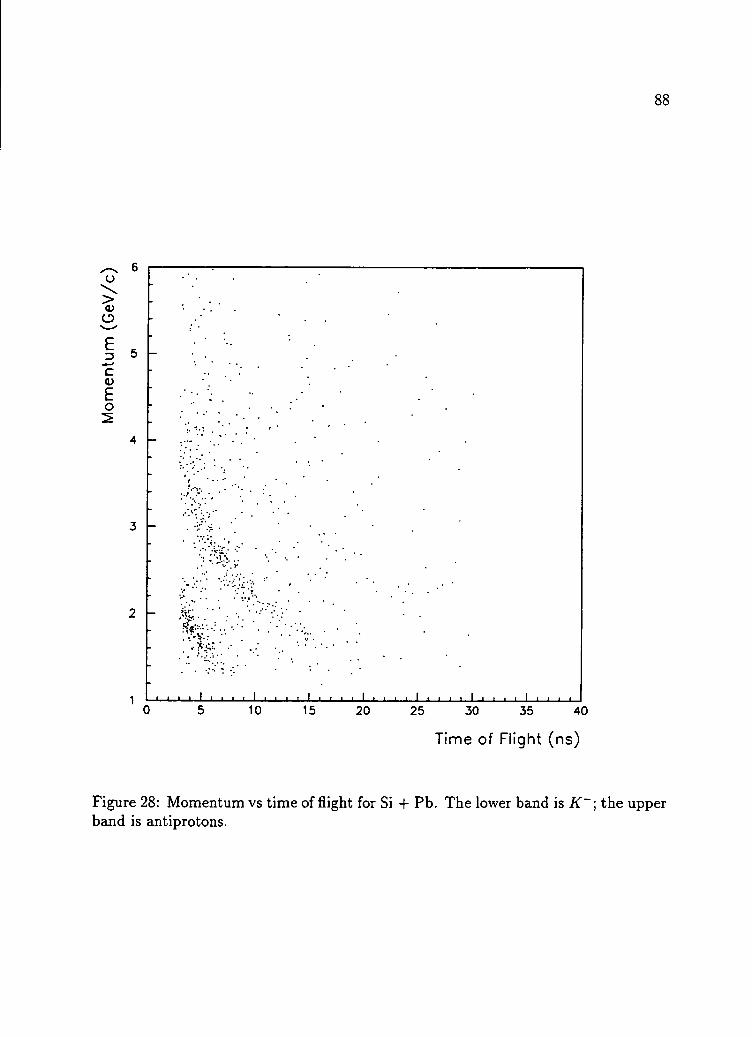
Time of Flight (ns)
Figure 28: Momentum vs time of flight for Si + Pb. The lower band is K ; the upperband is antiprotons.

89
between the measured time of flight and the true time of flight is given by:
^ tru e = ^measured "I" t v= c ( 6 . 3 3 )
where <,,=c is the time taken for a particle travelling at the speed of light to traverse
the same distance as the particle in question. Thus (3 is given by:
/3 = — ^ easured . (6.34)^measured "t" tv = c
Projections of m o m e n t u m and time of flight onto mass spectra for each of the three
targets are shown in Figure 29. These spectra show clear peaks for K ~ and for
antiprotons. Figure 30 shows the mass spectra after requiring the energy measured
in the calorimeter to be consistent with identification of the particle as an antiproton.
In order to estimate the background under the peak, the mass spectrum is integrated
from 1.18 to 2.14 GeV, the region adjacent to the mass peak. The level of background
is found to be 12% for the Pb and Cu targets, and 16% for the Al target. This fraction
is subtracted from the integral under the mass peak. All subsequent analysis is done
on the data having a reconstructed mass between .7 and 1.18 GeV.
As a verification of the Monte Carlo simulation of the experimental acceptance
(Section 2.7), a plot of transverse m o m e n t u m versus rapidity after applying all cuts
is made. Figure 31 shows the data from all three targets. Comparing this to Fig
ure 17, good agreement is found between the simulation and the measured antiproton
distributions.
6 . 2 C r o s s S e c t i o n s
The cross section a for an interaction is given by:
A'totai = o FaNSx (6.35)

3o3’c►1rt>tocosgcncnX>CDOc *p-1p>o’HCD
crCDc-t-er<->a>cd
number of countsK) O) oo
o o o o o
oCAv>c?£
mcd
100 Moss
(Ge
V/c
J) M
oss (G
eV
/c2)
nu m ber o f cou n ts
COo

number of counts
91
90c3Oo5 60jOE3C
30
Si +■ Cu
- J
-
L |
r
u
1 1 1 n rw,_
Moss (G e V /c J)2 3
Moss (G e V /c *)
Figure 30: Mass spectra for each of the three targets after applying the calorimeter energy requirement.

Tran
sver
se
mom
entu
m
(GeV
/c)
92
0.08
0.06
0.04
0.02
° 0 0.5 1 1.5 2 2.5 3
Rapidity
Figure 31: Accepted antiprotons as a function of transverse m o m e n t u m and rapidity.

93
where /Vtotai is the total number of interacted particles, F is the flux of incident
particles, a is the cross-sectional area of the beam or target, whichever is smaller, N
is the density of scattering centers, and Sx is the thickness of the target in the beam
direction [27]. If the beam is smaller than the target, F a — >• n;nc, the total number of
incident particles. The density of scattering centers, N , is given by:
N = (6.36)A
where p is the density of the target material, t is the target thickness, N a is Avogadro’s
number, and A is the mass number of the target nucleus. Thus, if we measure N meas
particles from a given reaction, the cross section for that reaction is:
eeflWmeas/lG = „ (6-37)Ti-incPt N a
with eeff being the total correction for measurement inefficiency.
In order to express the measured quantities in terms of yield per interaction, it
is necessary to divide the cross section above by the total nuclear interaction cross
section. This is given approximately by the geometric cross section:
a = 7r(Rp + Rt)2 (6.38)
where Rp and R t are the radius of the target and projectile nuclei. Using R = R qA 173
(Ro = 1.2 fm) we can evaluate the geometric cross section for a 28Si projectile incident
on Pb, Cu, and Al targets. The geometric cross sections for each of the three targets
are given in Table 9. W h e n calculating cross sections, it is useful to plot the cross
section in a Lorentz invariant form:
(Pa<7inv = (6.39)
or in terms of pt:
ffinv = » 1 f a, • (6.40)27rpt dptdy

94
Target Thickness (g/cm2) Cross Section (mb) Interaction Probability
Pb 11.3 3630 11.9%Cu 5.64 2240 11.9%Al 2.60 1650 9.6%
Table 9: The target thickness, calculated geometric cross section, and interaction probability are shown for Pb, Cu, and Al.
Table 10 shows the number of incident beam particles and double beam events, the
total number of interactions (with double beam events and background subtracted),
and the number of observed antiprotons for Pb, Cu, and Al targets.
A n examination of the data in Table 10 shows that the number of interactions
sampled is lower than expected for the Cu and Al targets, given the target thicknesses.
This is caused by the fact that the interaction threshold was fixed for all three targets.
Thus, 20% of the interactions in the Al target, and 10% of the interactions in the
Cu targets were not sampled. This inefficiency introduces a bias in the sample, since
the events lost are not distributed evenly over the entire interaction cross section,
but primarily in the more peripheral events. In order to correct for this effect, it was
assumed that all antiprotons were lost from events having a transverse energy below a
cut corresponding to 10% of the total production cross section for the Cu target, and
20% for the Al target. The number of antiprotons found below this cut was scaled
by the inefficiency. This resulted in a correction factor of 1.06 for the Al target, and
1.01 for the Cu target.
The relative yields of antiprotons per interaction in our data sample integrated
over all impact parameters for the three targets may be determined by scaling the
measured number of antiprotons by the number of interactions examined for each
target. Taking the antiproton yield for Pb to be 1, the relative yields for Pb:Cu:Al

95
Target Beam Double Beam Interactions Antiprotons
Pb 2.817 x 10⁸ 41154 3.345 x 10⁷ 276Cu 2.765 x 10⁸ 35214 3.287 x 10⁷ 266Al 3.451 x 10⁸ 32586 3.310 x 10⁷ 195
Table 10: The number of good beam particles and double beam events, total number of interactions, and observed number of antiprotons for Pb, Cu, and Al targets.
are 1:0.99:0.76 after correcting for the pretrigger inefficiencies, as discussed above. In
the discussion to follow, these yields will be considered in the context of a scaling
from proton-nucleus collisions.
For completeness, we can now plot t-da/dy, where e is the spectrometer acceptance
(see Figure 32). It is important to note that the pt acceptance is strongly rapidity-
dependent such that each rapidity bin corresponds to a different range in pt, as shown
in Figure 17. Thus the shape of these distributions is dominated by acceptance effects.
W e have measured the invariant cross section Ed^c/dp* at p t = 0 for different
rapidity intervals. Figures 33-35 show the results of these measurements for the Al,
Cu, and Pb targets.
The average values of these cross sections are given in Table 11. These numbers
have not been corrected for the finite time-of-flight resolution of the trigger.
These results can be compared to extrapolations to pt = 0 of the measurements
of Experiment E802 [17, 18]. For minimum bias Si + Al, a fit to data taken at higher
p t gives an extrapolated value for the invariant cross section of 6.6l|;3 m b • c3/ G e V 2
at y = 1.4. This is in reasonable agreement with the measured value of 5.6 ± 1.2
for the rapidity interval 1.3 > y > 1.5. For Si + Au, an extrapolation to p t = 0 at
y = 1.4 gives an invariant cross section of 25.7 1213• This is a factor of 2 higher than
the measured intercept for Si + Pb of 13.0 ± 2.5 for 1.3 > y > 1.5. Although the

e*dcr/dy (mb/unit of rapidity)
96
Figure 32: Rapidity distributions into the experimental acceptance for Al, Cu, andPb targets.

1/2np, da/dp,
1/2np, da/dp,
97
Transverse M om entum (G e V /c ) T ransverse M om entum (G e V /c )
Transverse M om entum (G e V /c ) T ransverse M om en tum (G e V /c )
Figure 33: The invariant cross section (in units of mb-c3/GeV2) for Si + Al as afunction of rapidity.

1 /2
np
, d
a/d
p,
1 /2
np
, d
a/d
p,
98
10'1.5 * y > 1.7
1 -
-110 I I I I . . . 1
Transverse M om entum (G e V /c )
0 0.02 0.04 0.06
T ransverse M om en tum (G e V /c )
T ransverse M om entum (G e V /c )
0 0.02 0.04 0.06
Tronsverse M om en tum (G e V /c )
Figure 34: The invariant cross section (in units of mb-c3/GeV2) for Si + Cu as afunction of rapidity.

99
ClT5t>■oae
Transverse M om entum (G e V /c )
0 0.02 0.04 0.06
Transverse M om en tum (G e V /c )
0 0.02 0.04 0.06
T ransverse M om en tum (G e V /c )
Figure 35: The invariant cross section (in units of mb-c3/GeV2) for Si + Pb as afunction of rapidity.

100
Rapidity Al Cu Pb1.3 < y < 1.5 5.5 ± 1.2 10.3 ±1.9 12.7 ±2.61.5 < y < 1.7 4.6 ±0.8 7.9 ±1.3 16.5 ±2.31.7 < y < 1.9 4.6 ±0.7 9.6 ±1.3 14.2 ± 2.01.9 < y < 2.1 1.2 ±0.4 3.2 ±0.7 5.4 ±1.3
Table 11: The invariant cross sections (in mb-c3/ G e V 2) for antiproton production at different rapidity intervals for Al, Cu, and Pb targets.
uncertainties in such an extrapolation are quite large, the discrepancy m a y suggest
a suppression of the antiproton yield at low transverse momentum. This would be
expected in the presence of absorption effects, since, on the average, the greatest
amount of target material must be traversed for a particle with low p t.
6 . 3 C e n t r a l i t y M e a s u r e s
In order to study the effects of different target nuclei on particle production, it is
desirable to study yield as a function of impact parameter. The reason for this
becomes clear if one considers the transverse energy spectrum for all collisions. In
the following section, an experimental definition of the transverse energy, E t, is given
and the relation of E t to collision geometry is discussed.
6.3.1 T r a n s v e r s e E n e r g y
For a detector consisting of n elements i, the transverse energy E t is
E t = ]T£;sin0i, (6.41)«=i
where E{ is the energy measured in the ith detector element located at an angle 0,
with respect to the target (see Figure 36).

101
Ei
Figure 36: A schematic representation of a detector used to determine transverse energy, E t. E; is the energy measured in detector element i.

102
Figure 37 shows the E t spectrum as measured using the target calorimeter for
those events which satisfy the pretrigger conditions for the Pb target. The shape of
this minimum bias distribution rougly reflects the geometry of the collision. Since
the probability for an interaction at impact parameter b goes as 2irbdb, the most
probable collisions Eire those at large impact parameter, yielding little transverse
energy. A study of particle production integrated over the minimum bias distribution
will be dominated by collisions taking place at large impact parameters where both
production and absorption are at a minimum. By using a measurement of the event
centrality, production can be studied in the region of more central collisions where
target effects are expected to be more significant.
Experiment 814 measures several quantities which are used for global event char
acterization. These quantities include transverse energy as discussed above, charged
particle multiplicity, and forward energy. Both the target calorimeter and participant
calorimeter are used to measure transverse energy. These measurements differ in the
pseodorapidity coverage (— 0.5 < rj < 0.8 for the TCAL, .83 < rj < 4.2 for the PCAL)
and also in that the T C A L allows more energy leakage. The raw number of struck
pads in the silicon multiplicity array is used as the measure of charged particle multi
plicity. During the antiproton running, the multiplicity array had intermittent noise
which caused many extra pads to register hits. Thus, the multiplicity distributions
exhibit more events at higher multiplicities than expected. These measurements are
shown for completeness; however, the two highest multiplicity bins are not reliable.
A n additional determination of event centrality is made by measuring the energy
which travels in the direction of the incident beam after the collision. The forward
energy is measured using the last wall of the uranium calorimeter. A sum is made
of the total energy deposited in a five stack section of the wall centered on the beam

da/dE
t milli
barn
s/GeV
103
S i + P b
Transverse Energy (GeV)
Figure 37: The minimum bias transverse energy distribution as measured by the target calorimeter for Si -f Pb collisions using the 11.9% Pb target. Distributions are also shown for data taken during the 1988 and 1991 runs using a 1.2% Pb target

104
calorimeter.
From the measured forward energy, Ef, an estimate can be made of the number
of nucleons that interacted in the target. If we assume that each of the surviving
nucleons carries the initial kinetic energy per nucleon of 13.6 GeV, the number of
interacted particles, nint, is
nint = 2 8 - ^ . (6.42)
The dependence of the background on centrality was determined assuming that
the behavior of the background in the region of the mass spectrum adjacent to the
antiproton peak is representative of the backrgound under the peak. Figure 38 shows
the background yield per interaction as a function of transverse energy. These yields
are measured for each of the centrality parameters and subtracted from the antiproton
yields per interaction in the subsequent analysis. Figures 39-40 show the correlations
among the various measures. Roughly, we find transverse energy and charged particle
multiplicity to be equivalent measures. The forward energy measurement (or equiva
lently, the number of interacted nucleons) provides a more sensitive measurement at
larger impact parameter, while the transverse energy distribution is useful at more
central collisions where the energy measurements are not dominated by fluctuations.
In comparing results among the three targets, it is important to note that the range
of impact parameters over which a collision might produce a given transverse energy
or multiplicity will depend on the target nucleus.
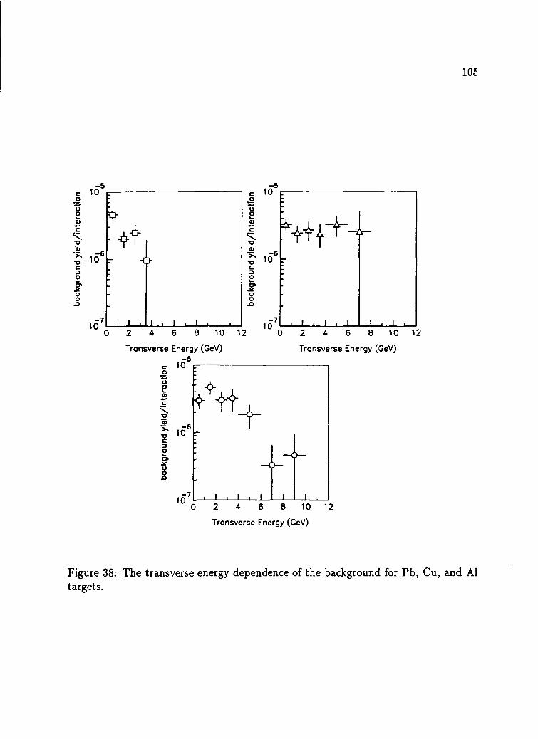
bock
grou
nd
yie
ld/i
nte
roc
tio
n105
-5
2 4 6 8 10 12
Transverse Energy (G eV)
Figure 38: The transverse energy dependence of the background for Pb, Cu, and Al targets.

Forw
ord
En
erg
y(G
eV)
0 2 4 6 0 2 4 6 TCAL E, (G eV) TCAL E, (G eV)
Figure 39: Correlations of T CAL transverse energy with multiplicity, PCAL transverse energy, forward energy, and number of interacted nucleons for Si + Al.

Forw
ord
En
erg
y(G
eV)
6 8TCAL E, (GeV)
TCAL E, (GeV)
6 8 TCAL E, (G eV)
28 - • .
Wv.>*v££^ ' ‘ 'T. • ' V .MG;- •
_L4 6 8
TCAL E, (G eV)
Figure 40: Correlations of T CAL transverse energy with multiplicity, PCAL transverse energy, forward energy, and number of interacted nucleons for Si + Cu.
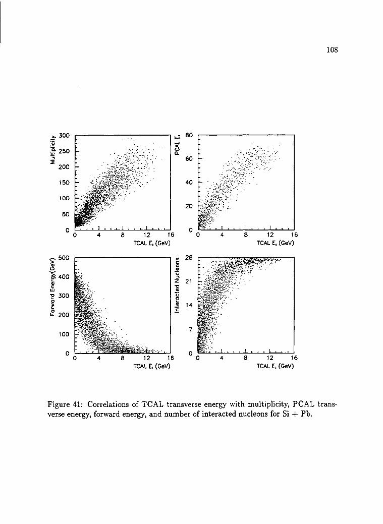
Forw
ord
En
erg
y(G
eV)
0 4 8 12 16 0 4 8 12 16TCAL E, (GeV) TCAL E, (GeV)
TCAL E, (G eV) TCAL E, (G eV)
Figure 41: Correlations of T CAL transverse energy with multiplicity, PCAL transverse energy, forward energy, and number of interacted nucleons for Si + Pb.

109
6 . 4 A n t i p r o t o n P r o d u c t i o n a s a F u n c t i o n o f C e n
t r a l i t y
Figures 42-56 show distributions of the centrality parameters discussed in the pre-
ceeding section for those events which produced an antiproton for 28Si incident on
each of the three targets. These figures also show the minimum bias (pretrigger) dis
tributions. It is more instructive, however, to plot the antiproton yield per interaction
as a function of event centrality. This is done by dividing the total antiproton yield
by the pretrigger spectrum, properly scaled. The results are shown in Figures 42-56.

110
-1 ^ 105oN.o _?6 10
(o) ontiprotons
R o to -3 •o 10
-410-A-
10 J I I I I I LU I I I I I I I I L
>VO\JOE
to•o
- 4
0 4 8 12 " 0 4 8 12
TCAL Transverse Energy (G eV) TCAL Tronsverse Energy (G eV)
TCAL Transverse Energy (G eV )
Figure 42: TCAL Transverse energy distributions for Si -f Al collisions, (a) TCALEt for those events which produced an antiproton, (b) Minimum bias TCAL Etspectrum, (c) Antiproton yield per interaction as a function of T CAL Et.

Ill
%oN■OE
(9*o
- A
0 4 8 12
TCAL Transverse Energy (GeV)
0 4 8 12
TCAL Tronsverse Energy (G eV)
TCAL Transverse Energy (G eV)
Figure 43: TCAL Transverse energy distributions for Si + Cu collisions, (a) TCALEt for those events which produced an antiproton, (b) Minimum bias TCAL Etspectrum, (c) Antiproton yield per interaction as a function of TCAL Et.

ontip
roto
n yi
eld
per
inte
ract
ion
da
/dE
, (m
b/G
eV
)112
r ■■■ - 10J\ (o) ontiprotons Lq _ (b) pretrigger
P'-o-.o.
O\.OEN_.UJT5\t>
102; -o-r! o - : -o-
■o 10 —: -6- -o-— T 1
iiiiny
_ i_i_i i i i i i i i t 1 i i i i i -110 ,._t .1. A 1 1 I 1 1 1 1 1 1 1 i 1 1 10 6 12 18 0 6 12 18
TCAL Transverse Energy (GeV) TCAL T ransverse Energy (G eV)
TCAL Transverse Energy (G eV)
Figure 44: TCAL Transverse energy distributions for Si + Pb collisions, (a) TCALEt for those events which produced an antiproton, (b) Minimum bias T C A L Etspectrum, (c) Antiproton yield per interaction as a function of TCAL Et.

ontip
roto
n yi
eld
per
inte
ract
ion
do
/dE
, (m
b/G
eV
)113
PCAL Transverse Energy (G eV) PCAL T ransverse Energy (G eV)
Figure 45: PCAL Transverse energy distributions for Si + Al collisions, (a) PCALEt for those events which produced an antiproton, (b) Minimum bias PCAL Etspectrum, (c) Antiproton yield per interaction as a function of PCAL Et■

antip
roto
n yi
eld
per
inte
ract
ion
da/
dE
, (m
b/G
eV
)114
10
103
10 -
10
-610
1 0 -' --------------------------1 (o) onliprotons $ { (b) pretrigger
o -s.o 1 0 2
A ~n‘ r - A -E ,—,uJT> 10 -A-
: -£r NbT5 ! - a -
1 1
\ t -110 r
■ i i i 1 i i i i 1 i i i i I i i i i - 210 1111 11 i ■ i 11111 i i
25 50 75
PCAL Tronsverse Energy (GeV)
100 25 50 75 100
PCAL Transverse Energy (G eV)
Figure 46: PCAL Transverse energy distributions for Si + Cu collisions, (a) PCALEt for those events which produced an antiproton, (b) Minimum bias PCAL Etspectrum, (c) Antiproton yield per interaction as a function of PCAL Et.

antip
roto
n yi
eld
per
inte
ract
ion
da/
dE
, (m
b/G
eV
)115
PCAL Transverse Energy (G eV) PCAL T ransverse Energy (G eV)
Figure 47: PCAL Transverse energy distributions for Si + Pb collisions, (a) PCALEt for those events which produced an antiproton, (b) Minimum bias PCAL Etspectrum, (c) Antiproton yield per interaction as a function of PCAL Et.

116
M ultiplicity M ultiplicity
M ultiplicity
Figure 48: Charged particle multiplicity distributions for Si + Al collisions, (a) Charged particle multiplicity for those events which produced an antiproton, (b) Minimum bias charged particle multiplicity spectrum, (c) Antiproton yield per interaction as a function of charged particle multiplicity. Note that the two highest multiplicity bins are not reliable measurements because of detector noise during the antiproton run.

117
Multiplicity
Figure 49: Charged particle multiplicity distributions for Si + Cu collisions, (a) Charged particle multiplicity for those events which produced an antiproton, (b) Minimum bias charged particle multiplicity spectrum, (c) Antiproton yield per interaction as a function of charged particle multiplicity. Note that the two highest multiplicity bins are not reliable measurements because of detector noise during the antiproton run.
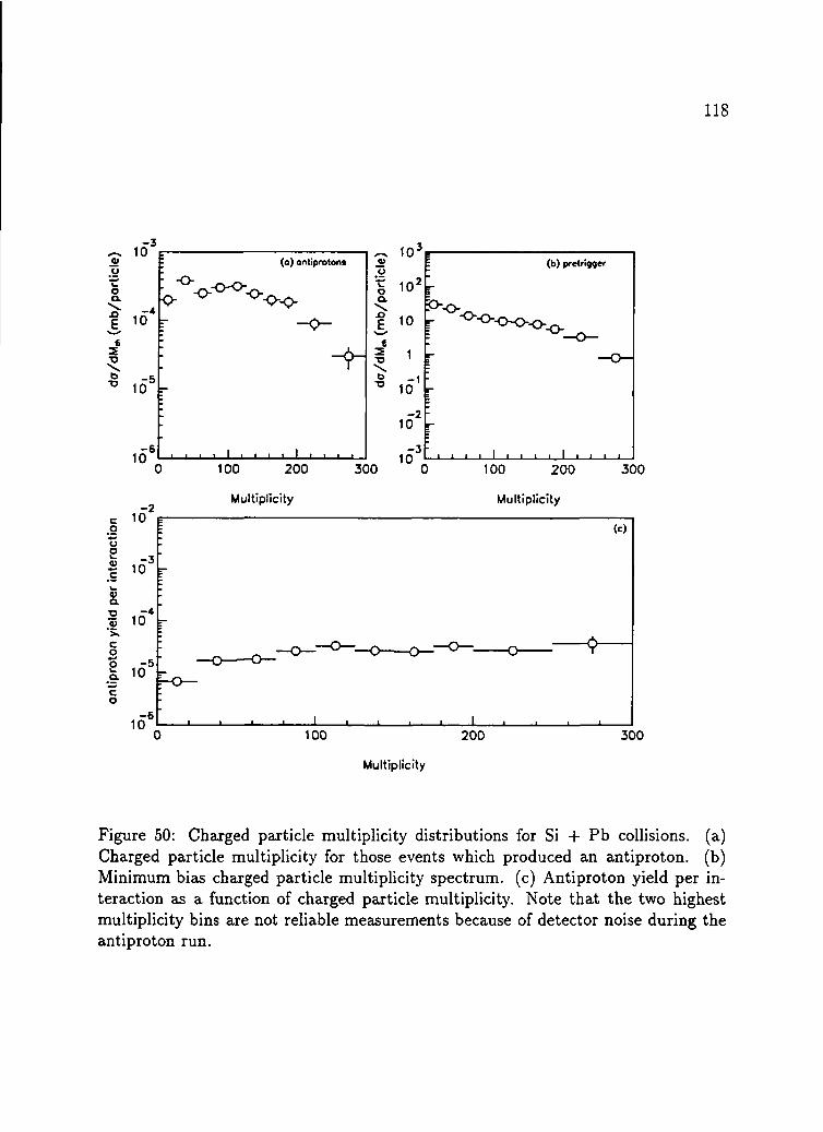
118
©ywoQ .\AEt2b"D
10 (o) ontiprotons
-410
io5
o
10 -I I I I I I L I
.s?OOCL
{2■oto "D
-2
100 200
Multiplicity
300
Multiplicity
Multiplicity
Figure 50: Charged particle multiplicity distributions for Si + Pb collisions, (a) Charged particle multiplicity for those events which produced an antiproton, (b) M inim um bias charged particle multiplicity spectrum, (c) Antiproton yield per interaction as a function of charged particle multiplicity. Note that the two highest multiplicity bins are not reliable measurements because of detector noise during the antiproton run.

antip
roto
n yie
ld pe
r int
erac
tion
da/dF
E (m
b/Ge
V)119
Forward Energy (GeV) Forward Energy (GeV)
Forword Energy (GeV)
Figure 51: Forward energy distributions for Si + Al collisions, (a) Forward energyfor those events which produced an antiproton, (b) Minimum bias forward energyspectrum, (c) Antiproton yield per interaction as a function of forward energy.

ontip
roton
yie
ld pe
r int
eroc
tion
da/dF
E (m
b/Ge
V)121
Forward Energy (GeV) Forward Energy (GeV)
Forward Energy (GeV)
Figure 53: Forward energy distributions for Si 4- Pb collisions, (a) Forward energyfor those events which produced an antiproton, (b) Minimum bias forward energyspectrum, (c) Antiproton yield per interaction as a function of forward energy.

ontip
roton
yie
ld pe
r int
erac
tion
do/dF
E (m
b/Ge
V)120
~ 10*| (o) ontiprolons > : (b) pretrigger■ o- > -
■ , A 1 10 r -A-- LUL. !^~^-A--A—A—A-”1 -A-
k
w\to 1X) 1 -
- r -1 -\ 10
i i i i i i i i i -210 --- 1--- 1--- 1--- L i 1 .A 1 1 10 250 500 0 250 500
Forward Energy (GeV) Forward Energy (GeV)
Figure 52: Forward energy distributions for Si + Cu collisions, (a) Forward energyfor those events which produced an antiproton, (b) Minimum bias forward energyspectrum, (c) Antiproton yield per interaction as a function of forward energy.

122
£u
-110(o) ontiprotons
O^ io2
\t>T3—4
10
10 l i t ! i . . . . i
_o>
u.0Q. \ £i
1 Z *o \ t> *D
-4
0 10 20
Number of interacted Nucleons Number of Interacted Nucleons
Number of Interocted Nucleons
Figure 54: Number of interacted nucleons for Si -f A l collisions, (a) N um ber of interacted nucleons for those events which produced an antiproton, (b) Num ber of interacted nucleons for minimum bias events, (c) Antiproton yield per interaction as a function of the number of interacted nucleons.

123
-1^ 104)O++wOn . _ *
(o) entiprotons
.O
E10 -
£ 103b■o
-A10
^ +
~ 10' o (b) pretrigger
OQ .\
.O
Ew
Jz■D\b■b
10* F£r : -A-
10 -
j 1 t l l l I l l 1. J I l » »0 10 20
-4 Number of Interacted Nucleons Number of Interacted Nucleons
Figure 55: Number of interacted nucleons for Si + Cu collisions, (a) Num ber of interacted nucleons for those events which produced an antiproton, (b) Num ber of interacted nucleons for minimum bias events, (c) Antiproton yield per interaction as a function of the number of interacted nucleons.

124
£o
-110(o) ontiprotons
10 -JOE
i io3NtoTO
-410
. O o 0
A
bOoQ .
b*o
-4 Number of Interacted Nucleons Number of Interacted Nucleons
Number of Interacted Nucleons
Figure 56: Number of interacted nucleons for Si + Pb collisions, (a) Num ber of interacted nucleons for those events which produced an antiproton, (b) Num ber of interacted nucleons for m inimum bias events, (c) Antiproton yield per interaction as a function of the number of interacted nucleons.

125
As a general trend, the antiproton yield per interaction does increase with event
centrality. This suggests that any absorption effects, expected to be greatest where
the largest amount of nuclear material must be traversed, do not completely dominate
the increase in production from the larger number of nucleon-nucleon collisions. In
considering the yield across the range of impact parameters, it is important to note
that the bias induced by the inefficiency of the pretrigger at peripheral Si + A l
collisions m ay cause the first points to be too high. A linear fit is made to each of the
curves in order to compare the general dependence of yield on centrality among the
targets. The slopes of these fits are given in Table 12. In each case, the Cu target
shows a slightly stronger centrality dependence than either A l or Pb. A comparison
of A l and Pb does not show a consistent trend, implying that target effects on the
centrality parameters are stronger than any target dependence on production.
The slopes of the forward energy curve, the centrality measure least affected by
rescattering in the target, shows no statistically significant differences among targets.
Even at the most central collisions, the antiproton yield per interaction does not
show a significant target dependence. In the absence of absorption of the antiprotons
within the target nucleus, one would naively expect to observe a greater production
in the heavier target from the larger number of nucleon-nucleon collisions. In the
following chapter, these expectations will be explored.

126
Parameter Al Cu PbT C A L E t 0.5 X 1 0 "6 0.3 X 10"-5 0.1 X io --5
P C A L E t 0.5 X 1 0 "7 0.9 X io --6 0.5 X io --6
Multiplicity 0.1 X 1 0 '6 0.4 X io --5 0.1 X io --6
Forward energy - 0 .8 X 1 0 '7 - 0 .1 X 10“-6 1 o to X io --7
int 0.1 X 1 0 "5 0.1 X io --5 0.1 X io --5
Table 12: Slopes o f linear fits to data of antiproton yield per interaction as a function of various centrality measures.

C h a p t e r 7
I n t e r p r e t a t i o n
In the previous chapter, the results from measurements of antiproton production at
pt = 0 were presented. In this chapter, the relative yields for the P b, Cu, and Al
targets are considered in the context of scaling from proton-nucleus collisions and
the implications of the centrality dependence is discussed. The antiproton yields as
a function of event centrality are described in terms of the simple collision picture
presented in the introduction in order to establish the effects of antiproton annihila
tion within the system after collision. A simple model of nucleus-nucleus collisions is
developed using the simple collision picture to further explore antiproton production
and absorption. Finally, existing measurements o f the antiproton transverse mo
m entum distributions are used with our measured intercepts to obtain extrapolated
Pt-integrated rapidity distributions.
7 . 1 R e l a t i v e Y i e l d s
Initial estimates o f antiproton yields may be m ade by attem pting to scale results
from proton-nucleus collisions. For this discussion, I use the results o f Sanford and
127
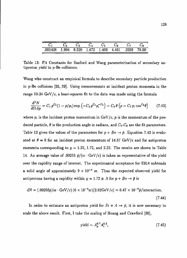
128
c x c2 c3 c4 c 5 c6 C7 c8.001426 1.994 9.320 1.672 1.480 4.461 .2026 78.00
Table 13: Fit Constants for Sanford and W ang parameterization of secondary antiproton yield in p-Be collisions.
W ang who construct an empirical formula to describe secondary particle production
in p-B e collisions [28, 29]. Using measurements at incident proton m om enta in the
range 10-34 G e V /c , a least-squares fit to the data was made using the formula
= C i PCi(l ~ P/Pi) exP ( “ C sPC*P~Cs) ~ C 6 0 (p - C 7 pi cosc*0) (7.43)
where p,- is the incident proton m omentum in G e V /c , p is the m om entum of the pro
duced particle, 6 is the production angle in radians, and C i-C s are the fit parameters.
Table 13 gives the values o f the parameters for p + J3e —» p . Equation 7.43 is evalu
ated at 6 = 0 for an incident proton m omentum of 14.57 G e V /c and for antiproton
m om enta corresponding to y = 1.22, 1.72, and 2.22. The results are shown in Table
14. A n average value of .00255 p / ( sr • G e V /c ) is taken as representative of the yield
over the rapidity range of interest. The experimantal acceptance for E814 subtends
a solid angle o f approximately 9 x 10⁻⁴ sr. Thus the expected observed yield for
antiprotons having a rapidity within y = 1.72 ± .5 for p + B e - * p is
dN = (.00255p /sr • G e V /c ) (6 x 10_4sr)(2 .8 2 G e V /c ) = 6 .47 x 10_6p/interaction.
(7.44)
In order to estimate an antiproton yield for S i + A -4 p, it is now necessary to
scale the above result. First, I take the scaling of Hoang and Crawford [30],
yield ~ A°p7A°'\ (7.45)

129
y Pd2JVdftdp
1.22 1.45 .001941.72 2.54 .003262.22 4.27 .00246
Table 14: Antiproton yield (in antiprotons per interaction per steradian per G e V /c ) in p -B e collisions for Pinc = 14.57 G e V /c from Sanford and W ang parameterization.
where A p and A t are the mass numbers of the projectile and target respectively.
Using this scale factor and equation 7.44, the yields can be calculated for Si + X -+ p
where X is Pb, Cu, or A l. These estimates are given in Table 15. It is instructive
first to compare the relative yields for the three targets. Taking the value for the
Pb target to be 1, the yields are 1:0 .79 :0 .66 (P b :C u :A l). The measured value is
somewhat higher yields for the Cu target and is in slightly better agreement for the
A l target. However, it is important to realize that for minim um bias interactions,
collision geometry dictates that most of the interactions will be fairly peripheral and
strong target effects m ay not be observed in the total yield. If the values for the
measured yields are compared directly to the scaling estim ates, these estimates are
found to be about a factor o f 8 higher than the measured values for all three targets.
Since the scaling is purely geometrical and does not take into account possible
absorption, it is possible that the lower measured yields indicate annihilation losses
on the order of 8 0 -9 0 % . A lso, such scaling allows antiproton production even after
a nucleon has undergone multiple collisions, which m ay lead to an overprediction of
the initial yield.
In order to take into account possible annihilation, a second scaling from the
Sanford and W ang yield estim ate will be made. A n estimate is made o f the mean free

130
Target Estimated p ’s per interaction Measured p ’s per interactionPb 1.3 x 1 0 -4 1.41 x 10“ 5Cu 1.0 x 1 0 '4 1.40 x 10“ 5Al 5.6 x 10” 5 1.07 x 10“ 5
Table 15: Antiproton yield in S i + X — > p (X is Pb, Cu, or A l) estimated using A^;7A 0t'2 scaling o f p + Be yield compared to measured yield into detector acceptance.
path, App, of a proton in normal nuclear matter,
= (7'46)
where N is the density of scattering centers and <t pp is the pp inelastic cross section.
Using
N = — — = 1.38 x 10⁻¹ nucleons • fm -3 (7 .47)4/ 37r (1.2/ m )3
and a ~ 30m b, a mean free path of 2.4 fm is found. Table 16 gives the diameters of
the target nuclei relative to App. Considering these results, the assumption is made
that only the nucleons on the surface of the projectile will interact in the target with
the full beam energy. A s a simple estim ate, the number o f interacting nucleons, n , is
taken to be7r(l.2A1/3)
" * ,(1 .2 ) ’ = A ■ (?'48)
So for a 28Si projectile, n « 9 .2. This approximation does not take into account
interactions at larger impact parameters, where not all o f the surface nucleons interact
in the target.
The annihilation cross section is taken from the parameterization by Koch and
Dover which gives

131
Target Radius(fm) D/\PPPb 7.1 5.9Cu 4.8 4.0Al 3.6 3.0
Table 16: Mean free path for a proton traversing the target nucleus
where
= 120 mb,
so = 4m^r = 3.52,
A = 50 M eV ,
B = 0.6.
For an antiproton produced at rapidity y = 1.7 and striking a proton as rest, the
center of mass energy is y /s = 2.64 G eV . Putting this into equation 7.49 gives
cdf = 37 m b . (7 .50)
Combining this value with Equation 7.47 gives a mean free path \ pp = 2 .0 fm for the
antiproton before annihilation.
Let lmax be the m axim um thickness of nuclear material the incident proton can
strike and still allow the produced antiproton to escape the target. Neglecting any
considerations of formation tim e,
lmax ~ App ± APP‘ (T.51)
Then there is a minimum impact parameter 6m:n where
hmin = y / R 2 ~ ( l m a x / 2 )2. (7 .52)

132
Target ^min / * ( % ) Estimated p ’s per interactionPb 6.8 10 5.7 x 1 0 '6Cu 4.3 21 1.3 x IO "5Al 2.9 37 2.2 x 1 0 "5
Table 17: Antiproton yield in Si + X —t p (X is P b, Cu, or A l) estimated assuming absorption of produced antiprotons
Antiprotons produced in collisions at 6 < 6min are not likely to escape the target
nucleus. This limits the fraction, f a of the total cross section available for antiproton
production to_ trR2 - trb2min
U = --- ^ --- • (7.53)
Taking the average yield per incident proton from Table 14, the projectile scaling of
9.2 incident nucleons, and assuming an available target cross section fraction f a , the
antiproton yield per interaction for 28S i+ P b is 5.7 x 10- 6 . In the absence of absorption,
this projectile scaling predicts a yield o f 6.0 x 10⁻⁵ antiprotons per interaction. A
comparison of these scaling estimates to the measured value of 1.4 x 10⁻⁵ suggests
that incorporating some absorption into scaling from proton-nucleus is necessary. O f
course, this treatment involves many approximations and should not be taken too
seriously. Table 17 shows the result of this calculation for Pb, Cu, and A l. The
estimated Cu and A l yields are still too high and this description predicts higher
yields per interaction with the lightest target which is not consistent with the data.

133
7 . 2 A S i m p l e M o d e l
7 .2 .1 D e v e lo p m e n t o f a S im p le M o d e l o f N u c le u s -N u c le u s
C o llis io n s
Initially, the target nucleus is generated using a Fermi density distribution :
'>(r) = l-t-exp[(r°— r„)/a„)]’ ( 7 M )
where r0 is the radius of the target nucleus and po and ao are constants determined
from electron scattering data [31]. The value of the density, p , is calculated as a
function of r, the distance from the center of the nuclear target.
The interaction of each projectile nucleon is treated separately; no collective effects
are considered. The initial position of the nucleon within the projectile nucleus is
generated using random distributions in r 2, 6, and 2n<j). For a given collision impact
parameter, the location of the projectile nucleon with respect to the target is then
determined. The projectile nucleon is propogated through the target in steps. After
each step, a check is made to determine whether the position of the particle is still
within the bounds of the target nucleus. If so, the density of the target nucleus at
the position of the projectile nucleon is determined using Equation 7.54. The target
density at the location of the next step is also found, and the average density, p ,between steps is used to evaluate the survival probability of the projectile at step i:
P ( i ) = exp -<Tppp , (7.55)
where <jpp is the proton-proton interaction cross section, taken to be 30 m b. A
random number uniformly distributed between 0 and 1 is generated; if this number
is above the survival probability, the projectile is considered to have interacted. The

134
propogation of the projectile nucleon through the target continues until it interacts
or escapes the target.
If the projectile nucleon undergoes a collision within the target, its proximity to
the surface o f the projectile nucleus is used to determine the probability that the
target nucleon has been struck for the first tim e. In this way, a distinction can be
m ade between the first, most energetic collisions, and subsequent interactions which
m ay have a lower available center-of-mass energy. For each collision that takes place,
the probability that the interaction produces an antiproton is estim ated, using a yield
of 0.0012 antiprotons per event [17]. The antiprotons are also produced with Gaussian
distrubuted rapidity and exponential transverse m om entum distributions as discussed
in Section 2.7.
If an antiproton is produced in the collision, it is first propogated freely through a
formation tim e r and then in steps through the target. T he method used is analagous
to that described above for the projectile nucleons. The K och-D over parametrization
(Equation 7.49) of the proton-antiproton annihilation cross section is used to estimate
the probability o f survival at each step. Those antiprotons which escape the target
nucleus are then sent through the experimental acceptance of the E814 apparatus
determined by the GEANT simulation as described in Section 2.7.
In order to compare the model calculations to the experimental results, the mea
sured parameters for event characterization are generated. The number of interacted
nucleons are simply counted. The T C A L transverse energy for the event is deter
mined by sampling a Gaussian distribution in E t per particle and sum m ing over all
interacted particles. Similarly, the charged particle multiplicity is generated using
the mean charged particle multiplicity per interacted particle. The m ean values and

135
E t &Et a m cH0.18 G e V /c 0.13 G e V /c 3.25 2.0
Table 18: The mean and width of the transverse energy ( E t /particle) and charged particle multiplicity distributions ( M ch /particle) used to generate event E t and charged particle multiplicity for the simple model.
widths of these distributions, as determined from data, are given in Table 18. Cor
rections are made to these distributions to allow for subsequent rescattering within
the target.
The energy produced at zero degrees is determined from a sum over surviving
projectile nucleons. Each nucleon is assumed to deposit its original kinetic energy of
13.6 G e V /c convolved with an additional Fermi energy distribution of width 2 .2 G eV .
The resulting energy is smeared by the measured forward calorimeter resolution.
7 .2 .2 R e s u lt s o f m o d e l c a lc u la t io n s
Before considering detailed results of the calculation of the centrality dependence of
antiproton yield, it is useful to use the results of the model to estimate any observed
antiproton absorption using the assumption of first-collision production. The mean
number of first collisions per interaction is found from the model calculations to be
3.5 ± 0 .4 , 4 .6 ± 0 .4 , and 6.3 ± 0.5 for Si + A l, Cu, and Pb respectively. From these
results and the measured antiproton yield per interaction, the antiproton yield into
the spectrometer acceptance can be calculated. The results of this calculation are
given in Table 19. In the absence of absorption, these results should be the same for
all targets, and comparable to the yield into the acceptance for the reaction p + p -> p. Taking the yield for this reaction to be 0.0012 antiprotons per proton-proton collision

136
Target p yield/interaction (Nfiret)/interaction p yield /first collisionA l 1.07 x 10⁻⁵ ± 0.08 x 1 0 "5 3.5 3.1 x 10~6 ± 0.2 x 1 0 '6Cu 1.40 x 10“ 5 ± 0 .0 9 x 10~5 4.6 3.0 x 1 0 "6 ± 0.2 x 1 0 "6Pb 1.41 x 10⁻⁵ ± 0.09 x 1 0 "5 6.3 2.2 x 10⁻⁶ ± 0.14 x 1 0 "6
Table 19: The antiproton yield into the E814 spectrometer acceptance for Si + A l, Cu, and Pb collisions, the mean number o f first collisions per interaction as calculated using a simple collision m odel, and the antiproton yield per first collision into the acceptance using the data and the model results.
into the experimental acceptance of 0 .4 % , an observed yield of 4 .8 x 10-6 antiprotons
per proton-proton collision is expected. The measured yields per first collision are
considerably lower than this value, with the greatest absorption being 54% of the
expected yield in the Pb target. In the Cu and A l targets, the absorption is estimated
to be 38% and 35% respectively. N ext, the calculated antiproton yield per interaction
into the acceptance is considered. Table 20 gives these results for production using
both the first-collision and all-collision production models. In all cases, it is found
that the measured yield is much lower than the values given under the assumption
that antiprotons are produced in all collisions, even for r = 1.5 fm . The calculation
employing first-collision production does a better job of reproducing the measured
yields; the data suggests that a r near 3.0 fm should be used.
The model results for the centrality parameters can now be exam ined. Figures 5 7 -
59 show the results of the model calculations of minim um bias distributions for T C A L
E t, charged particle multiplicity, forward energy, and number of interacted particles.
These calculations agree quite well with the data for E t for all three targets. The
charged particle multiplicity is also in reasonable agreement generally, although the
calculated distribution falls short of the measurement for the highest multiplicity
in the heaviest target. This is because the highest multiplicity measurements are

137
Target r (fm ) First collision A ll collisionsA l 1.5 9.0 X 1 0 -6 2.1 X 10~5Al 3.0 2.3 X 1 0 '5 4.5 X 10~5A l 6.0 2.5 X 10~5 4.7 X 10~5Cu 1.5 1.0 X 1 0 '5 2.3 X 10~5Cu 3.0 3.8 X 10~5 7.3 X lO’ 5Cu 6.0 4.6 X lO "5 8.6 X 10~5Pb 1.5 1.4 X 10~5 2.9 X 10~5Pb 3.0 5.7 X 1 0 "5 11.4 X 10“ 5Pb 6.0 9.7 X 10~5 19.0 X 10~5
Table 20: Calculated antiproton yield per interaction for A l, P b, and Cu targets and for formations times of 1 .5, 3 .0, and 6.0 fm .
138
affected by noise in the multiplicity array during the antiproton run (Section6.3.1).
T he forward energy calculation provides a good fit to the data except for the more
central collisions o f the A l target. The number of interacted nucleons, derived from
the forward energy measurement, shows the same discrepancies at the forward energy
plot; the linear scale serves to emphasize this.

139
C3Oo
Transverse Energy (GeV)
Figure 57: The solid lines give the results of the model calculations for the minimum bias transverse energy, charged particle multiplicity, forward energy, and number of interacted nucleons for Si + A l interactions. The plotted points are the pretrigger data. Note that the two highest multiplicity data points are not reliable measurements because of detector noise during the antiproton run.

140
10
- 10«
-O
E3C10
10
10
1 !-
1 ■ | | | I | | | ■ I | ■ | ■ I
Number of Interocted Nucleons
100 200 300 400 500
Forward Energy (GeV)
Figure 58: The solid lines give the results of the model calculations for the minimum bias transverse energy, charged particle multiplicity, forward energy, and number of interacted nucleons for Si + Cu interactions. The plotted points are the pretrigger data. Note that the two highest multiplicity data points are not reliable measurements because o f detector noise during the antiproton run.

141
C3O
4>£)3C
C3Ou
0)oE3C
Tronsverse Energy (GeV) Multiplicity
I i ■ ■ ■ I ■ » » ■ I » ■ * 1 I100 200 300 400 500
Forward Energy (GeV)
Figure 59: The solid lines give the results of the model calculations for the minimum bias transverse energy, charged particle multiplicity, forward energy, and number of interacted nucleons for Si + Pb interactions. The plotted points are the pretrigger data. Note that the two highest multiplicity data points are not reliable measurements because o f detector noise during the antiproton run.

142
N ext, the results for the calculation of the dependence of antiproton yield on event
centrality are examined and compared to the data. Figures 6 0 -8 3 show the calculated
antiproton yield per interaction into the experimental acceptance as a function of each
of the centrality parameters described above. For each target and measure o f central
ity, the calculated results for formation times r = 1.5, 3 .0 , and 6.0 fm axe superposed
with the data. Results are given with and without the assumption that the produc
tion occurs only during primary nucleon-nucleon collisions. A n initial examination of
these results shows the interplay between formation tim e and production exceeding
the first nucleon-nucleon collisions. Both a longer formation tim e and production
enhanced over the simple first collision picture lead to an increase in the observed
yield.
The A l data is reproduced fairly well using either all-collision production with
r = 1.5 fm or first-collision production with r = 3.0 fm . However, examination of all
three targets with both production pictures indicates that first-collision production
with a formation tim e near 3.0 fm best fits the general trend of the data.

Antip
roton
yield
pe
r int
erac
tion
(into
occe
pton
ce)
143
Figure 60: Calculated antiproton yield per interaction into the experimental acceptance as a function of transverse energy for Si -I- Al collisions. Formation times of1.5, 3.0, and 6.0 fm are assumed.

144
Transverse Energy (GeV)
Figure 61: Calculated antiproton yield per interaction into the experimental acceptance as a function of transverse energy for Si + A l collisions. Formation times of1.5, 3 .0 , and 6.0 fm are assumed. Antiproton production is assumed to occur only in first collisions between nucleons.

Antip
roton
yie
ld pe
r int
erac
tion
(into
occe
pton
ce)
145
Transverse Energy (GeV)
Figure 62: Calculated antiproton yield per interaction into the experimental acceptance as a function of transverse energy for Si + Cu collisions. Formation times of1.5, 3.0, and 6.0 fm are assumed.

146
Transverse Energy (GeV)
Figure 63: Calculated antiproton yield per interaction into the experimental acceptance as a function of transverse energy for Si Cu collisions. Formation times of1 .5, 3 .0, and 6.0 fm are assumed. Antiproton production is assumed to occur only in first collisions between nucleons.

Antip
roton
yie
ld pe
r int
erac
tion
(into
occe
pton
ce)
147
Transverse Energy (GeV)
Figure 64: Calculated antiproton yield per interaction into the experimental acceptance as a function of transverse energy for Si + Pb collisions. Formation times of1.5, 3.0, and 6.0 fm are assumed.

148
Figure 65: Calculated antiproton yield per interaction into the experimental acceptance as a function of transverse energy for Si + Pb collisions. Formation times of 1.5, 3 .0 , and 6.0 fm are assumed. Antiproton production is assumed to occur only in first collisions between nucleons.

Antip
roton
yie
ld pe
r int
erac
tion
(into
occe
pton
ce)
149
Figure 66: Calculated antiproton yield per interaction into the experimental acceptance as a function of charged particle multiplicity for Si + Al collisions. Formationtimes of 1.5, 3.0, and 6.0 fm are assumed.

150
Figure 67: Calculated antiproton yield per interaction into the experimental acceptance as a function of charged particle multiplicity for Si -I- A l collisions. Formation times of 1.5, 3 .0 , and 6.0 fm are assumed. Antiproton production is assumed to occur only in first collisions between nucleons.

Antip
roton
yie
ld pe
r int
eroc
tion
(into
occe
pton
ce)
151
Figure 68: Calculated antiproton yield per interaction into the experimented acceptance as a function of charged particle multiplicity for Si + Cu collisions. Formationtimes of 1.5, 3.0, and 6.0 fm are assumed.

152
Figure 69: Calculated antiproton yield per interaction into the experimental acceptance as a function of charged particle multiplicity for Si + Cu collisions. Formation times of 1.5, 3 .0 , and 6.0 fm are assumed. Antiproton production is assumed to occur only in first collisions between nucleons.

Antip
roton
yie
ld pe
r int
erac
tion
(into
acce
ptan
ce)
153
Figure 70: Calculated antiproton yield per interaction into the experimental acceptance as a function of charged particle multiplicity for Si -I- Pb collisions. Formationtimes of 1.5, 3.0, and 6.0 fm are assumed.

154
Figure 71: Calculated antiproton yield per interaction into the experimental acceptance as a function o f charged particle multiplicity for Si -f Pb collisions. Formation times of 1.5, 3 .0, and 6.0 fm are assumed. Antiproton production is assumed to occur only in first collisions between nucleons.

155
4>OcoQ .4)(JVo
1 o3O r = 6.0 fm □ r = 3.0 fm A r = 1.5 fm ■ Si + Al doto
co
4)a24)> sCooac<
-510
•At-- *
-A--tt-
rTT0m
10 J , ± t t I I i i i
100 200 300
Forward Energy (GeV)
400 500
Figure 72: Calculated antiproton yield per interaction into the experimental acceptance as a function of forward energy for Si + Al collisions. Formation times of 1.5,3.0, and 6.0 fm are assumed.
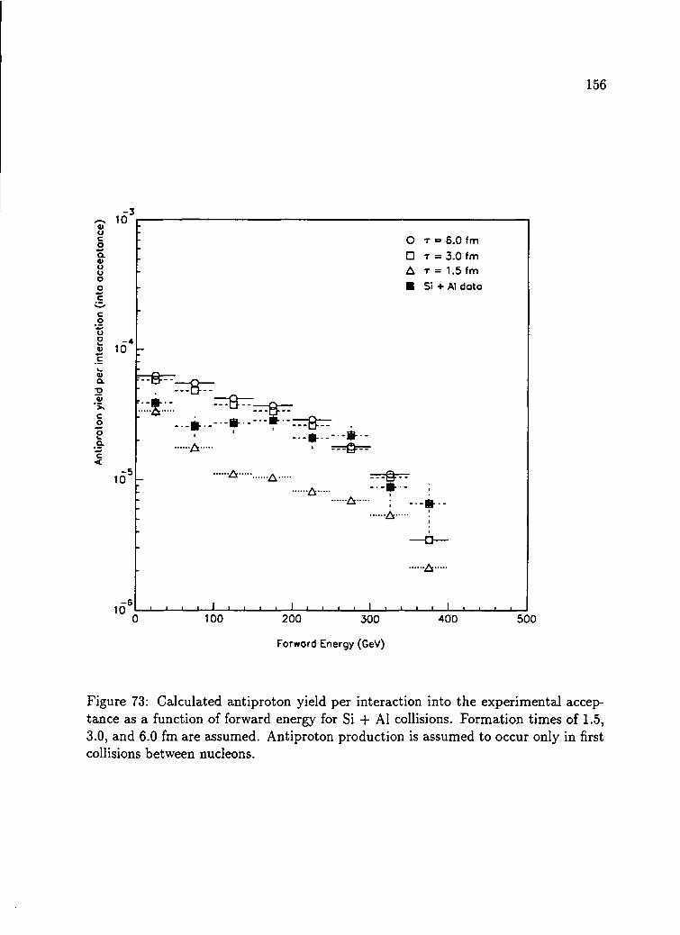
156
Figure 73: Calculated antiproton yield per interaction into the experimental acceptance as a function of forward energy for Si + A l collisions. Formation times o f 1.5, 3.0, and 6.0 fm are assumed. Antiproton production is assumed to occur only in first collisions between nucleons.

Antip
roton
yield
pe
r int
erac
tion
(into
occe
pton
ce)
157
Forword Energy (GeV)
Figure 74: Calculated antiproton yield per interaction into the experimental acceptance as a function of forward energy for Si + Cu collisions. Formation times of 1.5,3.0, and 6.0 fm are assumed.

158
Figure 75: Calculated antiproton yield per interaction into the experimental acceptance as a function of forward energy for Si + Cu collisions. Formation times of 1.5, 3.0, and 6.0 fm are assumed. Antiproton production is assumed to occur only in first collisions between nucleons.

Antip
roton
yie
ld pe
r int
erac
tion
(into
occe
pton
ce)
159
Figure 76: Calculated antiproton yield per interaction into the experimental acceptance as a function of forward energy for Si + Pb collisions. Formation times of 1.5,3.0, and 6.0 fm are assumed.
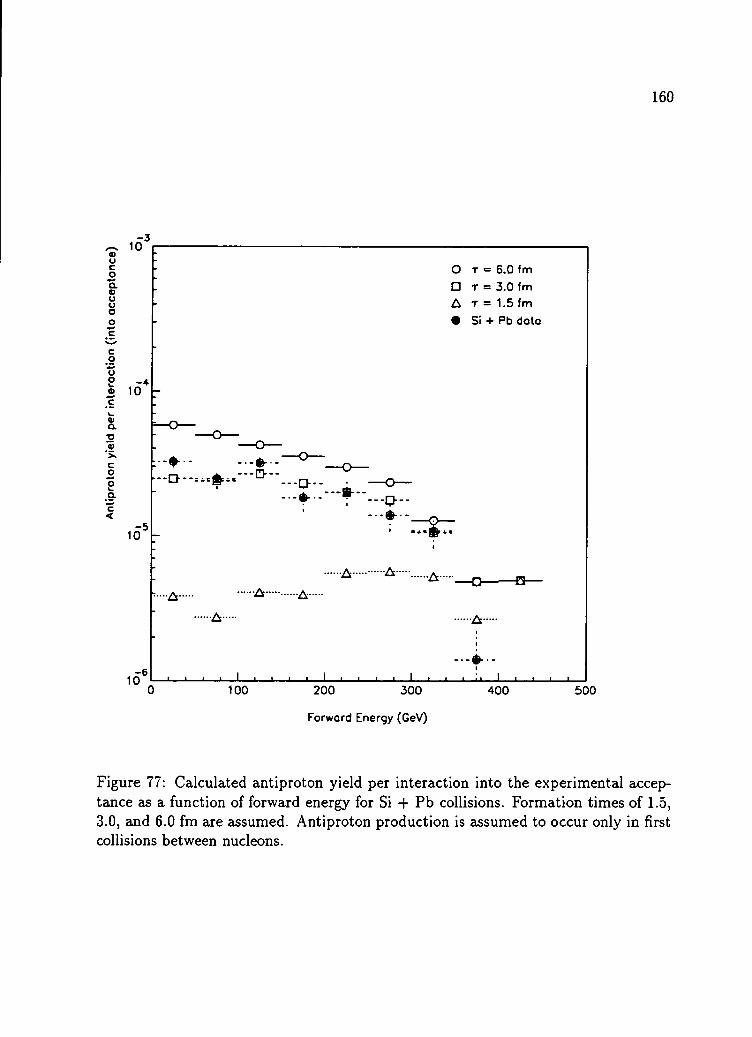
160
Figure 77: Calculated antiproton yield per interaction into the experimental acceptance as a function of forward energy for Si + Pb collisions. Formation times of 1.5, 3.0, and 6.0 fm are assumed. Antiproton production is assumed to occur only in first collisions between nucleons.

Antip
roton
yie
ld pe
r int
erac
tion
(into
occe
pton
ce)
161
Figure 78: Calculated antiproton yield per interaction into the experimental acceptance as a function of the number of interacted particles for Si + Al collisions. Formation times of 1.5, 3.0, and 6.0 fm are assumed.

162
Number of Interacted Nucleons
Figure 79: Calculated antiproton yield per interaction into the experimental acceptance as a function of the number of interacted particles for Si -+■ A l collisions. Formation times of 1.5, 3 .0, and 6.0 fm are assumed. Antiproton production is assumed to occur only in first collisions between nucleons.

Antip
roton
yie
ld pe
r int
erac
tion
(into
occe
pton
ce)
163
Figure 80: Calculated antiproton yield per interaction into the experimental acceptance as a function of the number of interacted particles for Si + Cu collisions.Formation times of 1.5, 3.0, and 6.0 fm are assumed.

164
0.12
0.09
0>ocopsQ .0)UUo
co3uoQ)psc0)aoa>c 0.06 oPSowQ .
c<
0.03
O t = 6.0 fm □ t = 3.0 fm A t = 1.5 fm ▲ Si + Cu data
--D-
Number of Interacted Nucleons
Figure 81: Calculated antiproton yield per interaction into the experimental acceptance as a function of the number of interacted particles for Si + Cu collisions. Formation times of 1.5, 3 .0, and 6.0 fm are assumed. Antiproton production is assumed to occur only in first collisions between nucleons.

Antip
roton
yie
ld pe
r int
eracti
on
(into
occe
pton
ce)
165
Number of Interacted Nucleons
Figure 82: Calculated antiproton yield per interaction into the experimental acceptance as a function of the number of interacted particles for Si + Pb collisions. Formation times of 1.5, 3.0, and 6.0 fm are assumed.

166
Figure 83: Calculated antiproton yield per interaction into the experimental acceptance as a function of the number of interacted particles for Si + Pb collisions. Formation times of 1.5, 3 .0, and 6.0 fm are assumed. Antiproton production is assumed to occur only in first collisions between nucleons.

167
The predictions of R Q M D [16] suggest that initial production of antiprotons may
be considerably enhanced over the first-collision model and balanced by a large
amount of subsequent absorption. By increasing the cross section for antiproton
production by a factor of 2.5 and using a short formation time (r = 1.5 fm ), the
interplay between increased production and absorption can be shown within the lim
itations o f this simple m odel. Figure 84 shows the result o f this calculation for each
o f the three targets. For the A l and Cu targets, the agreement with the data is good.
However, the amount o f absorption is overpredicted for the Pb target.
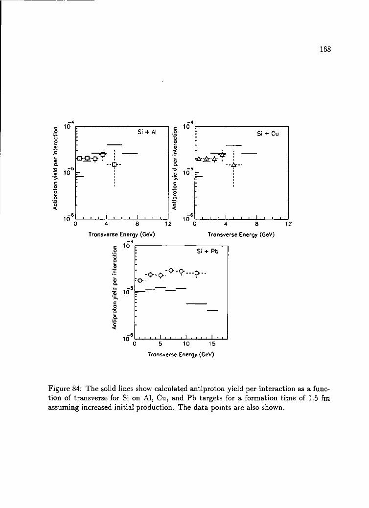
168
CoZo£Zw0)Q .
2fl>*>(coouq.Z<
coZow4)?u4>Q .
24>*XCoo
c<
Tronsverse Energy (GeV) Transverse Energy (GeV)
coZo0)ZOfQ .
2*> s
co**o2c<
Tronsverse Energy (GeV)
Figure 84: The solid lines show calculated antiproton yield per interaction as a function of transverse for Si on Al, Cu, and Pb targets for a formation time of 1.5 fmassuming increased initial production. The data points are also shown.

169
Finally, the antiproton yield per interaction as a function of the number of inter
acted nucleons is compared among each of the three targets. Figures 85-87 show the
results of the model calculations with the yield distributions for the different targets
superposed for the different values of t , with the assumption of production in first
collisions only. For r = 6.0 fm , the three targets are almost indistinguishable. A s the
formation tim e is decreased, the greater absorption in the heaviest target is mani
fested in reduced yield, with the target dependence being greatest at the m ost central
collisions. A similar plot of the data is shown in Figure 88 shows that the statistical
limitations of the data sample make it difficult to draw any conclusions about this
comparison, although the Pb data points do tend to lie below the A l data at higher
centrality.

Antip
roton
yie
ld pe
r int
erac
tion
(into
acce
ptan
ce)
170
0.5
0.4
0.3
0.2
0.1
° 0 4 8 12 16 20 24 28
Number of Interacted Nucleons
Figure 85: The calculated antiproton yield per interaction as a function of interactedparticles for Si on Al, Cu, and Pb targets for a formation time of 1.5 fm.
O Si + Pb A Si + Cu □ Si + Al
r = 1.5 fm-a -
-A ~
..... - - A — ' A r -
-A --
- -A-
- a -
■ » « i i i i i « « ■ i ■ J— J__ I I I I I l . .J.. . J I I 1 L_

Antip
roton
yie
ld pe
r int
erac
tion
(into
acce
ptan
ce)
171
Figure 86: The calculated antiproton yield per interaction as a function of interactedparticles for Si on Al, Cu, and Pb targets for a formation time of 3.0 fm.

Antip
roton
yie
ld pe
r int
erac
tion
(into
acce
ptan
ce)
172
Figure 87: The calculated antiproton yield per interaction as a function of interactedparticles for Si on Al, Cu, and Pb targets for a formation time of 6.0 fm.
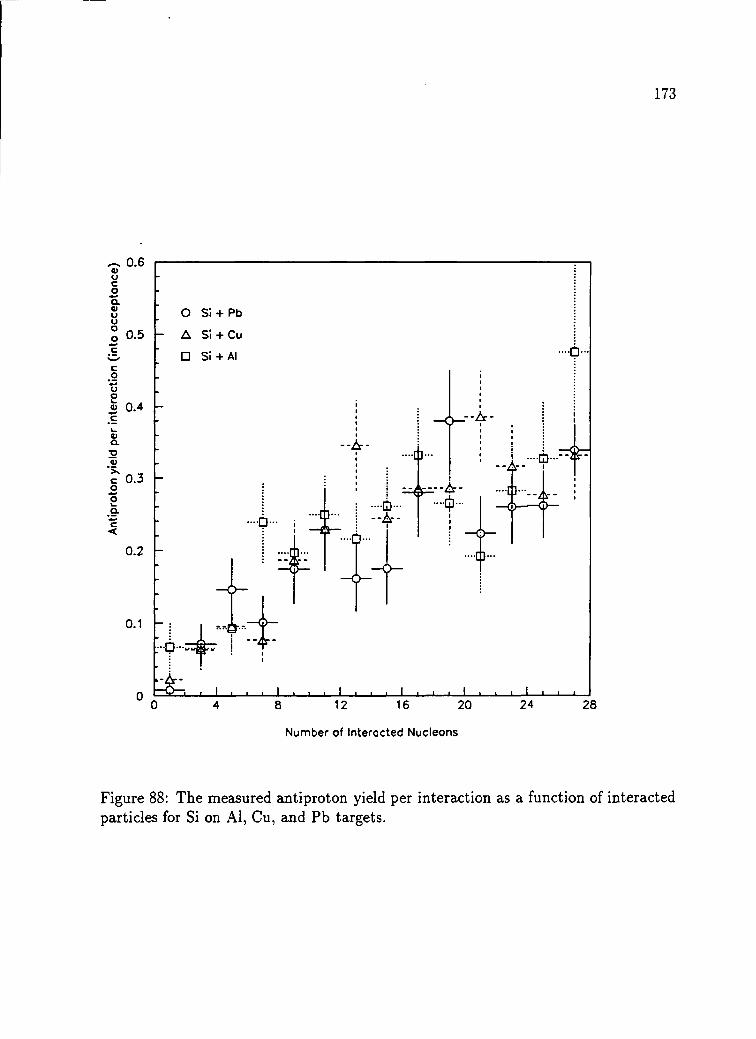
Antip
roton
yield
pe
r int
erac
tion
(into
occe
pton
ce)
173
Number of Interacted Nucleons
Figure 88: The measured antiproton yield per interaction as a function of interactedparticles for Si on Al, Cu, and Pb targets.

C h a p t e r 8
C o n c l u s i o n s
The E814 spectrometer has been used to study systematically the production of
antiprotons in interactions of 28Si at 14.6 G e V /c per nucleon with targets of A l, Cu,
and P b. The m inim um bias antiproton yields per interaction into the experimental
acceptance have been found to be 1.07 ± 0.9 x 10⁻⁵ for Si + A l, 1.40 ± 0.9 x 10⁻⁵ for
Si + Cu, and 1.41 ± 0.8 x 10⁻⁵ for Si -f Pb.
Invariant cross sections for antiproton production at zero transverse m om entum
have been measured for rapidities ranging from y = 1.3 to y = 2 .1. These results
axe compared to extrapolations of existing measurements at p t > 3 5 0 M e V /c from
Brookhaven Experiment 802 for minimum bias Si + A l and Si + A u collisions at
y = 1.4. The extrapolated intercepts are in good agreement with the measurements
described in this thesis for Si + A l. However, the invariant cross section measured
at p t — 0 by E814 for Si + Pb is a factor o f two lower than the value obtained by
extrapolating the Si + A u results of E802. W hile the errors in the extrapolation axe
large, this discrepancy m ay be indicative of absorption of low p t antiprotons within
the system after collision.
174

175
The antiproton yield per interaction is studied as a function of several measures
of event centrality, including transverse energy, charged particle multiplicity, and
forward energy. In the absence of absorption, production is expected to be greatest
in the heavier targets at the smallest impact parameters. The data does not indicate
increased yield with target at high centrality. The similarities in these distributions
among the different targets suggest that any increase in antiproton production in the
heavier targets is balanced by subsequent annihilation.
A simple collision model has been developed in order to evaluate possible ab
sorption effects. The results of this model calculation suggest that if antiprotons axe
produced only in primary collisions between nucleons, 3 5% , 3 8% , and 54% of these
antiprotons do not escape the A l, Cu, and Pb targets, respectively. Finally, the model
is used to generate distributions of antiproton yield per interaction as a function of
various centrality parameters. A comparison of the model results with the measured
distributions finds the best agreement to the data with a formation tim e near 3.0 fm
and antiproton production only in primary nucleon-nucleon collisions.
This study represents a beginning. Higher statistics clearly are needed, as well
as measurements over the entire range o f transverse m om entum . Such measurements
should include a determination of event centrality in order to fully explore the effects
of the different targets.
These measurements serve to establish the effectiveness of antiproton production
as a probe of the hot dense environment produced in relativistic heavy ion collisions.
Once produced, the antiprotons do interact within the system . Evaluated in the
framework of increasingly sophisticated collision models, measurements of antiproton
production should provide detailed information about the evolution o f the collision
in space and time.

A p p e n d i x A
P h o t o m u l t i p l i e r s a n d E l e c t r o n i c s
Detector Photomultiplier Signal ProcessingOffline Trigger
T C A L N /A LeCroy 1882 A D C LeCroy 4300B F E R AT P A D Thorn E M I 9127B LeCroy 1882 A D C Philips 7106 discr.M U L T N /A LeCroy P C O S 2735 LeCroy 4300B F E R A
LeCroy P C O S 2732P C A L Thorn E M I 9954AD R C H N /A LeCroy 1885 A D C N /A
LeCroy 1879 T D C N /AFSCI Thorn E M I 9954B LeCroy 1885 A D C LeCroy 4300B F E R A
LeCroy 4290 T D C LeCroy 4303 F E R E TU C A L Philips X P 2081 LeCroy 1882 A D C LeCroy 4300B F E R A
LeCroy 4290 T D C
Table 21: Photomultipliers and Signal Processing Electronics
176

B i b l i o g r a p h y
[1] See, for example, proceedings from the International Conference on U ltra -
Relativistic Nucleus-Nucleus Collisions, Nucl. Phys. A 4 9 8 (1 9 8 9 ) (Quark M atter
’88) and Nucl. Phys. A 5 2 5 (1 9 9 1 ) (Quark M atter ’89).
[2] F. Karsch, in Q u a r k -G lu o n P la sm a , edited by R. C. Hwa (W orld Scientific
Publishing Company, 1990).
[3] M . Jacob, Nucl. Phys. A 4 9 8 , lc (1989).
[4] T . A . DeGrand, Phys. R ev. D 3 0 , 2001 (1984).
, [5] E. W itten , Phys. Rev. D 3 0 , 272 (1984).
[6] U . Heinz, P. R . Subramanian, and W . Greiner, Z. Phys. A 3 1 8 , 247 (1984).
[7] K . S. Lee, M . J. Rhoades-Brown, and U . Heinz, Phys. Rev. C 3 7 , 1452 (1988).
[8] J. Ellis and U. Heinz, Phys. Lett. B 2 3 3 , 223 (1989).
[9] S. Gavin, M . Gyulassy, M . Piimer, and R. Venugopalan, Phys. Lett. B 2 3 4 , 175
(1990).
[10] S. Gavin, Nucl. Phys. A 5 2 5 , 459c (1991).
177

178
[11] J. D . Bjorken, Phys. Rev. D 2 7 , 140 (1983).
[12] J. Barrette e t a l., Phys. Rev. Lett. 6 4 , 1219 (1990).
[13] J. Barrette e t al, Phys. Rev. C 4 5 , 819 (1992).
[14] H. Sorge, H. Stocker, and W . Greiner, Ann. Phys. (N .Y .) 1 9 1 , 266 (1989).
[15] H. Sorge, A . von K eitz, R . M attielo, H. Stocker, and W . Greiner, Nucl. Phys.
A 5 2 5 , 95c (1991).
[16] A . Jahns, H. Stoocker, W . Greiner, and H. Sorge, Phys. Rev. Lett. 6 8 , 2895
(1992).
[17] J. B . Costales, PhD thesis, Massachusetts Institute of Technology, 1990.
[18] T . A bbott et al, Phys. Lett. B 2 7 1 , 447 (1991).
[19] M . Aoki e t a l., in press.
[20] L. W aters, PhD thesis, State University o f New York, Stony Brook, 1990.
[21] R . Debbe et a l., IE E E Trans, on Nucl. Sci. 3 7 , 88 (1990).
[22] J. Fischer et a l., IE E E Trans, on Nucl. Sci. 3 7 , 82 (1990).
[23] S. V . Greene et a l., Nucl. Phys. A 5 2 5 , 369c (1991).
[24] G. Alverson et al, V A X O N L I N E V 2 .1 , Fermilab, 1987.
[25] R . Brun et al., G E A N T V ers io n 3 .1 4 , C E R N Data Handling Division, 1987,
D D /E E /8 4 -1 .
179
[26] P. R . Bevington, D a ta re d u c tio n a n d e r ro r a n a ly s is f o r th e p h y s ic a l sc ie n c e s (M cG raw -H ill Book Company, 1969).
[27] W . R. Leo, T ech n iq u es f o r n u c le a r a n d p a r tic le p h y s ic s e x p e r im e n ts (Springer-
Verlag, 1987).
[28] J. R . Sanford and C . L. W ang, E m p ir ic a l fo r m u la s f o r p a r tic le p r o d u c tio n in P - B e c o llis io n be tw een 10 a n d 3 5 B e V /c , Internal Report B N L 11299 (Brookhaven
National Laboratory, 1967).
[29] J. R . Sanford and C . L. W ang, E m p ir ic a l fo r m u la s f o r p a r tic le p ro d u c tio n in P - B e c o llis io n be tw een 10 a n d 3 5 B e V /c , Internal Report B N L 11479 (Brookhaven
National Laboratory, 1967).
[30] T . Hoang and H. Crawford, Phys. Rev. D 4 2 , 45 (1990).
[31] M . A . Preston and R . K . Bhaduri, S tr u c tu r e o f th e N u c le u s (A ddison-W esley
Publishing Company, Inc., 1975).