Geology and Geophysics Applied to Groundwater Hydrology at Fort Irwin, California

David C. Buesch, Editor

Gravity Survey and Interpretation of Fort Irwin and Vicinity, Mojave Desert, California

By R.C. Jachens and V.E. Langenheim

Open-File Report 2013–1024–H

U.S. Department of the Interior U.S. Geological Survey

U.S. Department of the Interior SALLY JEWELL, Secretary

U.S. Geological Survey Suzette M. Kimball, Acting Director

U.S. Geological Survey, Reston, Virginia: 2014

For more information on the USGS—the Federal source for science about the Earth, its natural and living resources, natural hazards, and the environment—visit http://www.usgs.gov or call 1–888–ASK–USGS (1–888–275–8747)

For an overview of USGS information products, including maps, imagery, and publications, visit http://www.usgs.gov/pubprod

To order this and other USGS information products, visit http://store.usgs.gov

Any use of trade, firm, or product names is for descriptive purposes only and does not imply endorsement by the U.S. Government.

Although this information product, for the most part, is in the public domain, it also may contain copyrighted materials as noted in the text. Permission to reproduce copyrighted items must be secured from the copyright owner.

Suggested citation: Jachens, R.C., and Langenheim, V.E., 2014, Gravity survey and interpretation of Fort Irwin and vicinity, Mojave Desert, California, chap. H of Buesch, D.C., ed., Geology and geophysics applied to groundwater hydrology at Fort Irwin, California: U.S. Geological Survey Open-File Report 2013–1024, 11 p., http://dx.doi.org/10.3133/ofr20131024H.

ISSN 2331-1258 (online)

iii

Contents Abstract ...................................................................................................................................................................... 1 Introduction ................................................................................................................................................................. 1 Datasets ..................................................................................................................................................................... 1

Gravity Surveys and Reduction ............................................................................................................................... 1 Geologic Data ......................................................................................................................................................... 2 Data-Point Constraints on Thickness of Basin Fill ................................................................................................... 2

Gravity Field................................................................................................................................................................ 2 Thickness of Cenozoic Deposits Estimated from Gravity Data ................................................................................... 4 Acknowledgments ....................................................................................................................................................... 4 References Cited ........................................................................................................................................................ 4

Figures

1. Simplified geologic map of Fort Irwin and vicinity over shaded-relief topography .......................................... 6 2. Isostatic residual gravity map of Fort Irwin and vicinity .................................................................................. 7 3. Basement gravity map of Fort Irwin and vicinity ............................................................................................. 8 4. Basin gravity map of Fort Irwin and vicinity .................................................................................................... 9 5. Map showing depth to basement beneath Fort Irwin and vicinity ................................................................. 10

Tables

1. Density-depth function. ................................................................................................................................ 11

Supplemental Data

1. Gravity survey data [Available online only at http://pubs.usgs.gov/of/2013/1024/h/.]

iv

Conversion Factors SI to Inch/Pound

Multiply By To obtain

Length meter (m) 3.281 foot (ft)

kilometer (km) 0.6214 mile (mi)

Density

kilogram per cubic meter (kg/m3) 0.06242 pound per cubic foot (lb/ft3)

Gravity Survey and Interpretation of Fort Irwin and Vicinity, Mojave Desert, California

By R.C. Jachens and V.E. Langenheim

Abstract In support of a hydrogeologic study of the groundwater resources on Fort Irwin, we have

combined new gravity data with preexisting measurements to produce an isostatic residual gravity map, which we then separated into two components reflecting (1) the density distribution in the pre-Cenozoic basement complex and (2) the distribution of low-density Cenozoic volcanic and sedimentary deposits that lie on top of the basement complex. The second component was inverted to estimate the three-dimensional distribution of Cenozoic deposits by using constraints from geology, drillholes, and time-domain electromagnetic soundings. In most of the base, the Cenozoic deposits are no more than 300 m thick, except in the basins with more than 500 m of fill beneath Coyote Lake, Red Pass Lake, west of Nelson Lake, west of Superior Lake, Bicycle Lake, and in the vicinity of Nelson Lake.

Introduction We have conducted a gravity investigation of Fort Irwin, Mojave Desert, California (fig. 1), in

support of a comprehensive study of the hydrology and groundwater resources of the base. Other components of the study included analyses of geology, aeromagnetic surveys, airborne electrical surveys, ground-based time-domain electromagnetic (TEM) soundings, drillholes, and water-quality sampling.

The main goal of the gravity investigation was to provide a preliminary view of the distribution of alluvial basins, shapes, areal extents, and approximate thicknesses of alluvial fill. The gravity interpretation used constraints from geology, drillholes, TEM soundings, and aeromagnetic surveys to provide derivative products for integration with other data. Derivative products include separation of the gravity field into two components: that caused by density variations in the basement complex and that caused by the distribution of Cenozoic fill, along with a three-dimensional representation of the thickness of the Cenozoic fill.

Datasets Gravity Surveys and Reduction

For this investigation, gravity point data were compiled from the reports by Snyder and others (1982) and the Pan-American Center for Earth and Environmental Studies (2010), as well as from 976 new gravity observations collected specifically for the hydrologic study of the Fort Irwin (fig. 2). The gravity data were reduced by using the Geodetic Reference System of 1967 (International Association of Geodesy and Geophysics, 1971) and referenced to the International Gravity Standardization Net 1971 gravity datum (Morelli, 1974, p. 18). Gravity data were reduced to isostatic anomalies by using a

2

reduction density of 2,670 kg/m3, and including earth-tide, instrument drift, free-air, Bouguer, latitude, curvature, and terrain corrections (Telford and others, 1976; LaFehr, 1991). An isostatic correction using a sea-level crustal thickness of 25 km and a mantle-crust density contrast of 400 kg/m3 was applied to the gravity data to remove the long-wavelength gravitational effect of isostatic compensation of the crust due to topographic loading (Jachens and Roberts, 1981). The data were gridded at a spacing of 250 m, using a minimum-curvature algorithm. The resulting gravity field is termed the “isostatic residual gravity anomaly.”

Terrain corrections, which were computed to a radial distance of 166.7 km, involved a 3-part process: (1) Hayford-Bowie zones A and B with an outer radius of 68 m were estimated in the field with the aid of tables and charts, (2) Hayford-Bowie zones C and D with an outer radius of 590 m were computed by using a 30-m digital elevation model, and (3) terrain corrections from a distance of 0.590 to 166.7 km were calculated by using a digital elevation model and the procedure of Plouff (1977). Total terrain corrections for the stations within the study area ranged from 0 to 82.7 milligals (mGal), averaging 1.1 mGal. Only 14 percent of the stations in the study area (figs. 1, 2) have terrain corrections greater than 5 mGal, mostly in the mountains north and east of Fort Irwin. Fewer than 20 stations within Fort Irwin (dashed line in fig. 2) have terrain corrections greater than 5 mGal. If the error resulting from a terrain correction is considered to be 5 to 10 percent of the total terrain correction, the largest error from the terrain correction expected for nearly all the data from within Fort Irwin is 0.5 mGal; however, the error resulting from the terrain correction is small (< 0.1 mGal) for most stations within Fort Irwin owing to low relief.

Geologic Data

Geologic data from three sources were used to define the surface geology within the study area (fig. 1). The primary source was the geologic map by Jennings and others (1962) at a scale of 1:250,000. We upgraded the geologic information within Fort Irwin on the basis of more recent geologic mapping at a scale of 1:250,000 by the California Geological Survey (G. Saucedo, unpub. data, 2011). For remote areas where data were unavailable on these two maps, additional data were obtained from the Geologic Map of California (Jennings and others, 1977), at a scale 1:750,000.

Data-Point Constraints on Thickness of Basin Fill

Three types of data were used to constrain the inversion of the gravity data in order to provide a regional estimate of the thickness of the basin fill: drillholes, seismic profiles, and TEM soundings. A total of 8 drillholes that penetrated the crystalline basement were available for this study (fig. 1); data from 18 other drillholes that did not penetrate basement were used only to establish that the results of the gravity inversion agreed with the drillhole data. Two shallow seismic profiles provided information on the basement depth in the Langford Basin (fig. 1). Finally, interpretations from 18 TEM soundings (see Burgess and Bedrosian, this volume, chap. F), 9 of which were interpreted to indicate the likely depth to basement, also were compared with the gravity results to ensure consistency between interpretations of the two types of data.

Gravity Field The gravity field in the study area (fig. 2; here expressed as the isostatic residual gravity field) is

complex, reflecting two major classes of density variations: those within the pre-Cenozoic basement rocks, and those resulting from the three-dimensional distribution of low-density Cenozoic volcanic and

3

sedimentary deposits that lie on top of the basement rocks. The method for separating these two components is discussed in the next section.

The gravity field caused by density variations within the basement complex (called the basement gravity field) is shown in figure 3. The main feature of this field is a central gravity low that extends from the Granite Mountains westward and southwestward across the study area, corresponding to outcrops of low-density Cretaceous granitic rocks (fig. 1). Low-density plutons are a common feature of much of the Mojave Desert region. These plutonic gravity lows, which are surrounded by gravity highs more characteristic of the Death Valley country north and northeast of the study area, correspond to complex assemblages of older Mesozoic and older igneous, metamorphic, and sedimentary rocks (Jennings and others, 1962).

Superposed on this basement gravity field is a secondary gravity field (called the basin gravity field) that reflects the three-dimensional distribution of Cenozoic volcanic and sedimentary deposits, which are significantly lower in density than the underlying basement rocks. This field is shown in figure 4.

The thickness of the Cenozoic basin-filling deposits (or depth to the basement complex) throughout the study area (fig. 5) was estimated by using the method of Jachens and Moring (1990), modified to permit inclusion of constraints at points where the thickness of the Cenozoic deposits is known from direct observations in boreholes or from other geophysical measurements. This method was shown to be effective by Phelps and others (1999) in determining the general configuration of the pre-Cenozoic basement in Nevada, where they compared calculated basin depths with data from densely spaced drillholes. An initial estimate of the basement gravity field was made by passing a smooth surface through the gravity values measured at stations where rocks of the basement complex crop out, and subtracting this value from the isostatic residual gravity field to yield an initial estimate of the basin gravity field. This estimate is only initial because the gravity values at points on the basement complex that lie close to the Cenozoic deposits are influenced by the gravity effect of these lower-density deposits and are therefore lower than they would be if the Cenozoic deposits were absent. To compensate for this effect, the initial basin gravity field was used to calculate an initial estimate of the thickness of the Cenozoic deposits, and the gravity effect of these deposits was calculated at all basement gravity stations. A second estimate of the basement gravity field is then made by passing a smooth surface through the basement gravity values corrected by the effects of the nearby Cenozoic deposits, and the process was repeated to obtain a second estimate of the thickness of the Cenozoic deposits. This process was repeated until further steps resulted in no significant changes to the modeled thickness of the Cenozoic deposits, generally with five or six iterations.

The basin gravity field was converted to the thickness of the Cenozoic deposits by using an assumed density contrast that varies with depth (table 1) between the Cenozoic sedimentary and volcanic deposits and the underlying basement complex. This density-depth relation, which is the same as that used by Saltus and Jachens (1995) for estimating the thickness of Cenozoic deposits throughout the Great Basin/Mojave Desert of the Western United States, was based on in situ density estimates derived from borehole gravity surveys. The resulting density contrast of 650 kg/m3 for the Cenozoic sedimentary deposits in the upper 200 m is reasonable for Quaternary continental deposits overlying Mesozoic and older crystalline rocks. Use of this entire density-depth relation in areas with a substantial thickness of Cenozoic volcanic deposits may lead to a systematic underestimate of the thickness of the basin fill. The reasonableness of this selection of density contrast was further tested by examining the basement gravity field for any indications of local anomalies at the few sites where drill-holes penetrated the basement complex and the solution was forced to fit those data.

4

Thickness of Cenozoic Deposits Estimated from Gravity Data The estimated thickness of Cenozoic deposits (depth to pre-Cenozoic basement) is shown in

figure 5. The estimate is based on a constrained inversion of the gravity data, as described in the previous section. A critical element in such an inversion is accurate knowledge of the density of the Cenozoic deposits relative to the density of the basement rocks. This knowledge typically requires a large set of drillholes that penetrate the entire Cenozoic section, borehole density logs, borehole gravity surveys, borehole sonic velocity logs, or some combination of these datasets. Unfortunately, only a few drillholes are available within Fort Irwin, and none of these other data types that are reliable exist to our knowledge. Therefore, we were forced to use density information obtained from data in other parts of the Great Basin.

The lack of density data specific to basins in Fort Irwin (fig. 1) introduces an uncertainty into the resulting estimates of the depth to basement. This uncertainty primarily takes the form of imprecise depths to basement, not in the general shapes of the basins or their distribution. Thus, the deep basins in figure 5 are shown in their proper locations, and their boundaries are correct, but the exact depth to basement beneath them is uncertain.

With those limitations in mind, in most of Fort Irwin, the Cenozoic deposits are no more than 300 m (1,000 ft) thick. Large basins deeper than 1,000 m (3,300 ft) occur beneath Coyote Lake, Red Pass Lake, and west of Nelson Lake. The deep basin west of Nelson Lake appears to be filled mostly with Tertiary volcanic deposits. Smaller basins from 500 m (1,500 ft) to 800 m (2,500 ft) deep occur west of Superior Lake, beneath Bicycle Lake, and in the vicinity of Nelson Lake. Large expanses covered by a thin blanket of probable Quaternary alluvium characterize most of the rest of Fort Irwin.

Acknowledgments We gratefully acknowledge financial support from Fort Irwin. We thank Andy Morita, Jim

Howle, and Bob Carruth for their efforts in collecting gravity data. We also thank Dave Ponce and Jeffrey Lucius for their helpful and thorough reviews.

References Cited Burgess, M.K., and Bedrosian, P.A., 2014, Time-domain electromagnetic surveys at Fort Irwin, San

Bernardino County, California, 2010–12, chap. F of Buesch, D.C., ed., Geology and geophysics applied to groundwater hydrology at Fort Irwin, California: U.S. Geological Survey Open-File Report 2013–1024 (this volume).

International Association of Geodesy, 1971, Geodetic Reference System 1967: International Association of Geodesy Special Publication 3, 116 p.

Jachens, R.C., and Moring, B.C., 1990, Maps of thickness of Cenozoic deposits and the isostatic residual gravity over basement for Nevada: U.S. Geological Survey Open-File Report 90-404, scale 1:1,000,000.

Jachens, R.C., and Roberts, C.W., 1981, Documentation of a FORTRAN program, “isocomp”, for computing isostatic residual gravity: U.S. Geological Open-File Report 81–574, 26 p.

Jennings, C.W., Burnett, J.L., and Troxel, B.W., compilers, 1962, Trona sheet of Geologic map of California: California Division of Mines and Geology, scale 1:250,000.

Jennings, C.W., Strand, R.G., and Rogers, T.H., compilers, 1977, Geologic map of California: California Division of Mines and Geology, scale 1:750,000.

5

LaFehr, T.R., 1991, Exact solution for gravity curvature Bullard B correction: Geophysics, v. 56, no. 8, p. 1179–1184.

Morelli, C., ed., 1974, The international gravity standardization net 1971: International Association of Geodesy Special Publication 4, 194 p.

Pan-American Center for Earth and Environmental Studies, 2010, Gravity database: accessed January 8, 2010, at http://irpsvgis00.utep.edu/repositorywebsite.

Phelps, G.A., Langenheim, V.E., and Jachens, R.C., 1999, Thickness of Cenozoic deposits of Yucca Flat inferred from gravity data, Nevada Test Site, Nevada: U.S. Geological Survey Open-File Report 99-310, 33 p.

Plouff, D., 1977, Preliminary documentation of a FORTRAN program to compute gravity terrain corrections based on topography digitized on a geographic grid: U.S. Geological Survey Open-File Report 77-535, 45 p.

Saltus, R.W., and Jachens, R.C., 1995, Gravity and basin depth maps for the Basin and Range province, Western United States: U.S. Geological Survey Geophysical Map GP-1012, scale 1:2,500,000.

Snyder, D.B., Roberts, C.W., Saltus, R.W., and Sikora, R.F., 1982, A magnetic tape containing the principal facts of 64,026 gravity stations in the state of California: available from U.S. Department of Commerce, National Technical Information Service, document PB 82-168287, 34 p.

Telford, W.M., Geldart, L.O., Sheriff, R.E., and Keyes, D.A., 1976, Applied Geophysics: New York, Cambridge University Press, 860 p.

6

Figure 1. Simplified geologic map of Fort Irwin (outlined by dashed black line) and vicinity over shaded-relief topography. Geology from Jennings and others (1962, 1977).

7

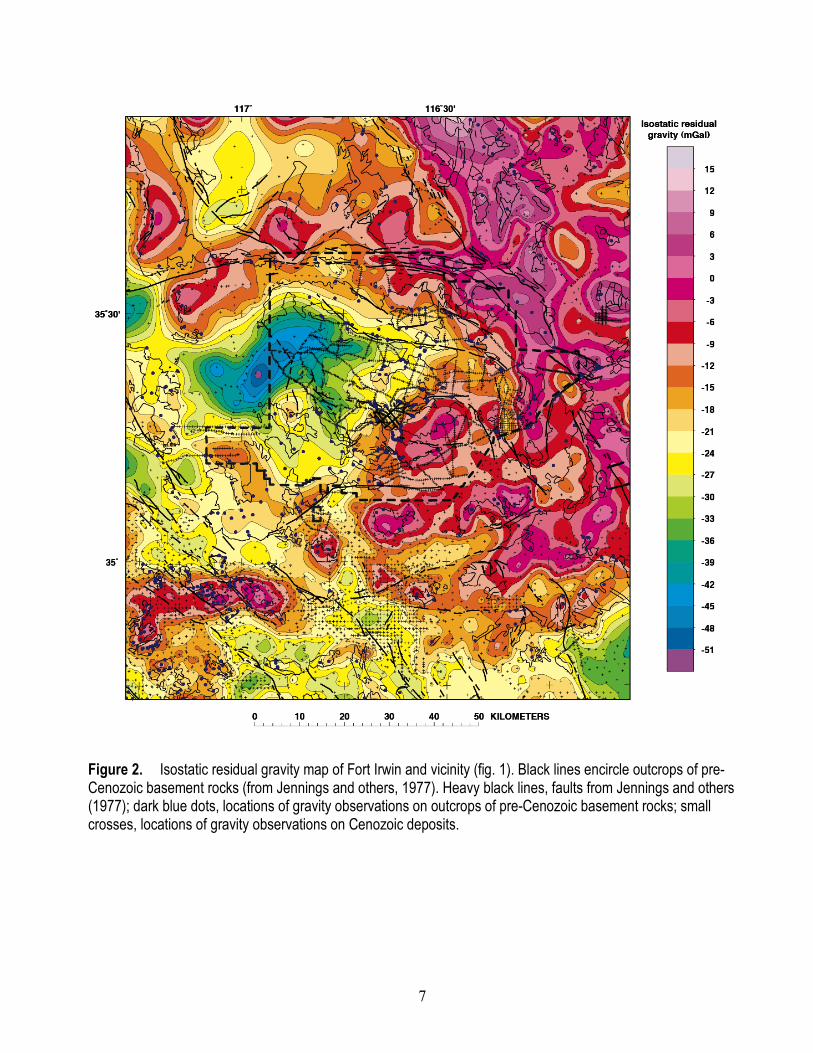
Figure 2. Isostatic residual gravity map of Fort Irwin and vicinity (fig. 1). Black lines encircle outcrops of pre-Cenozoic basement rocks (from Jennings and others, 1977). Heavy black lines, faults from Jennings and others (1977); dark blue dots, locations of gravity observations on outcrops of pre-Cenozoic basement rocks; small crosses, locations of gravity observations on Cenozoic deposits.

8

Figure 3. Basement gravity map of Fort Irwin and vicinity (fig. 1). Black lines encircle outcrops of pre-Cenozoic basement rocks (from Jennings and others, 1977). See figure 2 for explanation of lines and symbols.

9

Figure 4. Basin gravity map of Fort Irwin and vicinity (fig. 1). Black lines encircle outcrops of pre-Cenozoic basement rocks (from Jennings and others, 1977). See figure 2 for explanation of lines and symbols.

10

Figure 5. Map showing depth to basement beneath Fort Irwin and vicinity. Black lines encircle outcrops of pre-Cenozoic basement rocks (from Jennings and others, 1977); red lines encircle outcrops of Cenozoic volcanic deposits (from Jennings and others, 1977). Heavy black lines, faults (from Jennings and others, 1977); dark blue dots, locations of gravity observations on outcrops of pre-Cenozoic basement rocks; small crosses show locations of gravity observations on Cenozoic deposits; white triangles, locations of drillholes or seismic soundings that indicated depth to basement; red triangles, places where data were artificially constrained during inversion to prevent inferred basement from cropping out where no basement outcrops have been mapped.

11

Table 1. Density-depth function.

Depth (m)

Density contrast (kg/m3)

0–200 -650 200–600 -550

600–1,200 -350 >1,200 -250