Gravity Lab & Intro Problems Review - West Virginia...

Tom Wilson, Department of Geology and Geography

Environmental and Exploration Geophysics II

tom.h.wilson

[email protected]

Department of Geology and Geography

West Virginia University

Morgantown, WV

Gravity Lab & Intro Problems Review


time dial

reading

Converted to

milliGals

relative

difference

Tide &

Drift

Drift

corrected

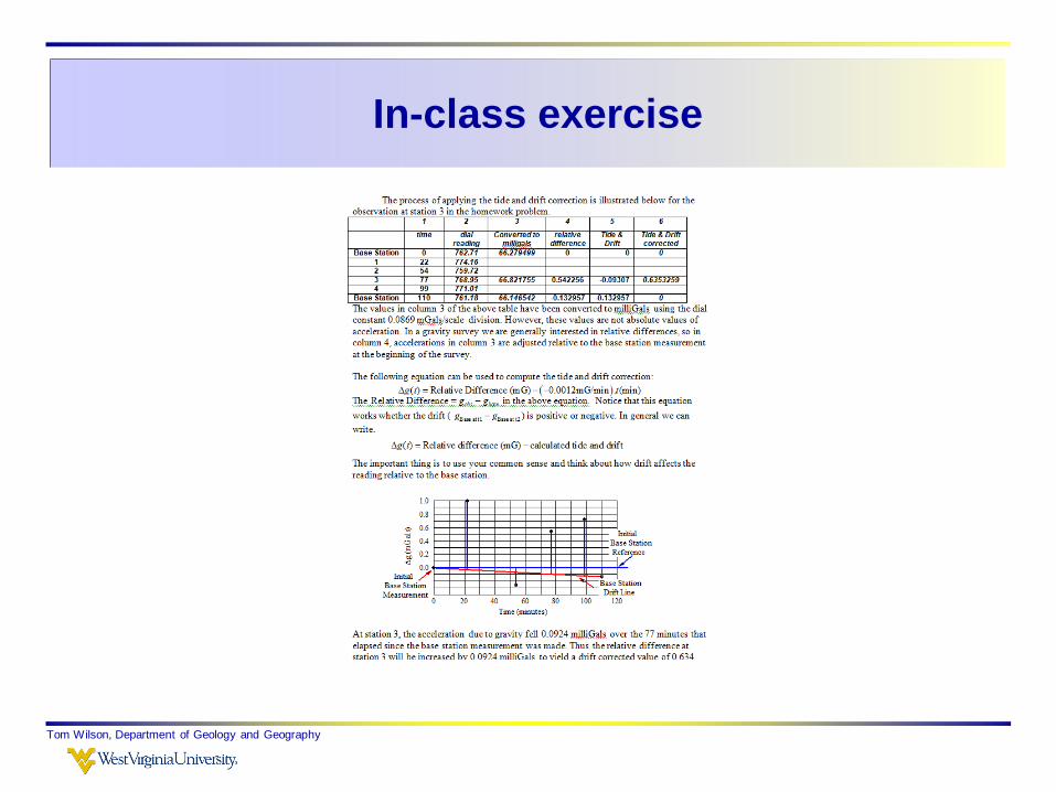
Base Station 0 762.71 66.279499 0 0 0

1 22 774.16

2 54 759.72

3 77 768.95 66.821755 0.542256 -0.09307 0.635326

4 99 771.01

Base Station 110 761.18 66.146542 -0.132957 -0.13296 0

Getting the answer


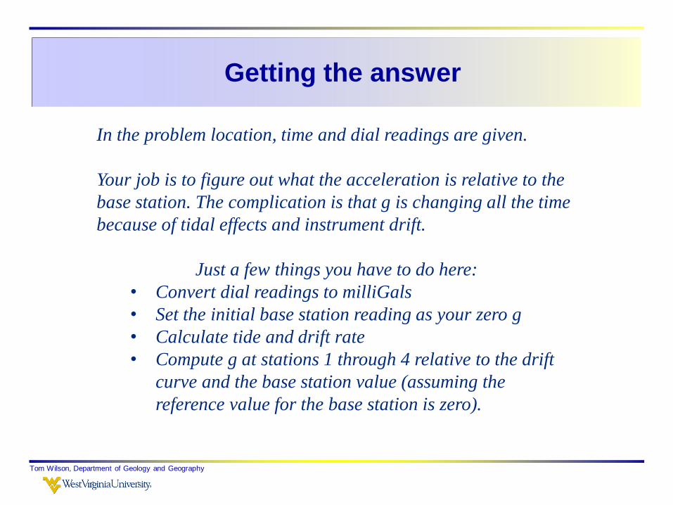
In the problem location, time and dial readings are given.

Your job is to figure out what the acceleration is relative to the

base station. The complication is that g is changing all the time

because of tidal effects and instrument drift.

Just a few things you have to do here:

• Convert dial readings to milliGals

• Set the initial base station reading as your zero g

• Calculate tide and drift rate

• Compute g at stations 1 through 4 relative to the drift

curve and the base station value (assuming the

reference value for the base station is zero).

What’s the tide and drift rate


time dial

reading

Converted to

milliGals

relative

difference

Tide &

Drift

Drift

corrected

Base Station 0 762.71 66.279499 0 0 0

1 22 774.16

2 54 759.72

3 77 768.95 66.821755 0.542256 -0.0931 0.635326

4 99 771.01

Base Station 110 761.18 66.146542 -0.132957 -0.13296 0

66.147 66.28 0.1330.0012

110 110 min

g mG

t

Carry calculations out to 3 decimal places

Tide and drift rate

Prepare a drift curve. Values are shown relative to a base station

value of 0. The visual graphical reference is very helpful. It makes

it clear what your result should be station-by-station


Time (minutes)

0 20 40 60 80 100 120

g (

mG

als)

-0.4

-0.2

0.0

0.2

0.4

0.6

0.8

1.0

Base Station

Drift Line

Initial

Base Station

Reference

Initial

Base Station

Measurement

Station 3 measurement is 66.822 mG. It’s value relative to the base is

+0.542

3

With tide and drift rate of -0.0012 mG/min the difference

of station 3 relative to the base is increased.

The following equation can be used to

compute the tide and drift correction:

( ) Relative Difference (mG) 0.0012mG/min . (min)g t t

Relative Difference = obs baseg g

this equation works whether the drift is positive or negative

( ) Relative difference (mG) calculated tide and driftg t

To use the example from the table

Station 3


The relative difference = gobs – gbase (at 8) = 66.822-66.28=0.542mGThe actual difference, g(t), can then be calculated as

( ) 0.542 ( 0.0012 *77min)min

mGg t

This value differs a little from that in the table due to a little more rounding.

( ) Relative difference (mG) calculated tide and drift (mG)g t

( ) 0.542 0.0924 0.6344g t mGals

In-class exercise



Then … Back to the gravity labStewart’s plate approximation and the

impact of edge effects


Stewart uses different conversion factors to convert inputs in

different units to obtain

gt 130

This expression comes directly from tGg plate 2

Stewart has solved it using a density = -0.6 gm/cm3. He has also included the factor which transforms centimeters to feet so that the user can input t in units of feet. g is in units of milligals.

where t is in feet130

tg or

What are the implications of the negative density contrast on the resulting gravity anomalies?

Refer to results of

your in class problem


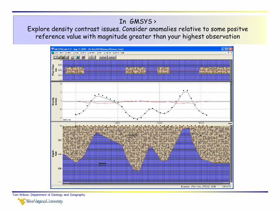
In GMSYS >Explore density contrast issues. Consider anomalies relative to some positve

reference value with magnitude greater than your highest observation

Or set the DC Shift to absolute 0



• Open up the upper pane, set the plan view depth; • specify a pattern. • Note how the upper pane fills out. • Do the same for the bedrock.• Adjust plan view depth again• Change range on Plan View scale.

Extending your model into the 3rd dimension

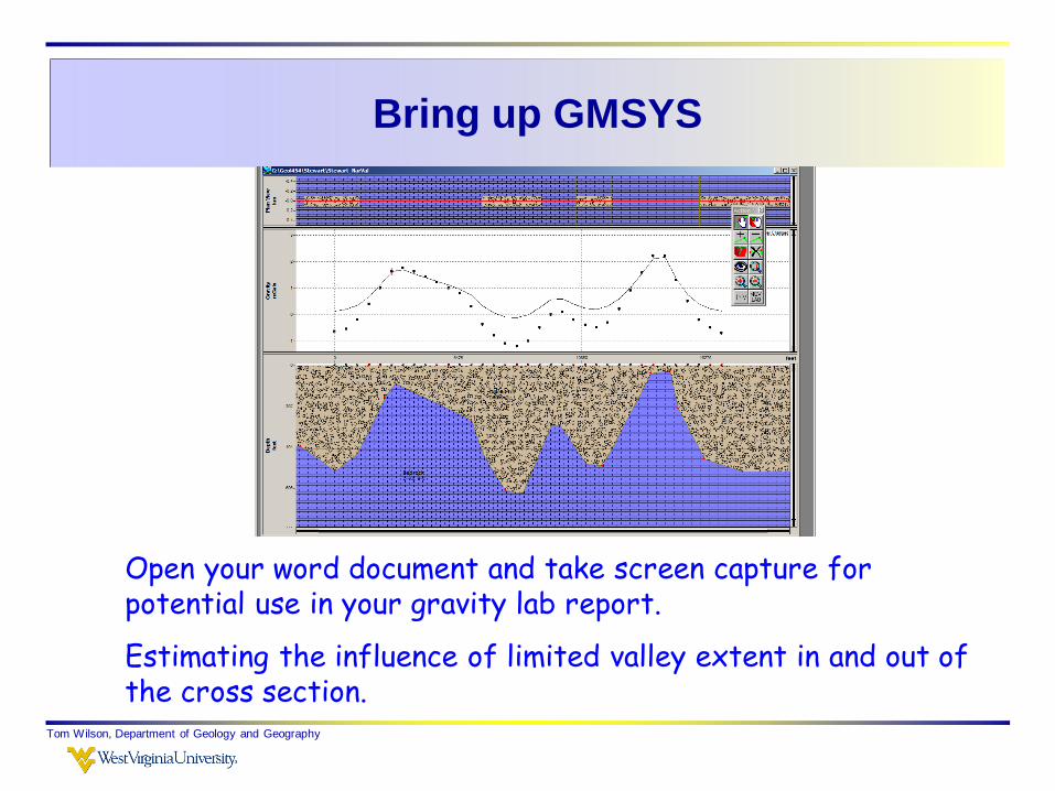
Bring up GMSYS


Open your word document and take screen capture for potential use in your gravity lab report.

Estimating the influence of limited valley extent in and out of the cross section.


Follow the standard reporting format. Include the following or similar subdivisions:

Abstract: a brief description of what you did and the main result(s) you obtained (~200 words).Background: Provide some background on the purpose of the survey, the data we’re analyzing... All of this would come from Stewart’s paper. Explain the approximation he uses and answer question 1 below in this section to illustrate his approach.Results: Describe how you tested the model proposed by Stewart (the one we are reworking in the lab). Include answers to questions 2 through 4 below in this results discussion.Conclusions: Summarize the highlights of results obtained in the forgoing modeling process.


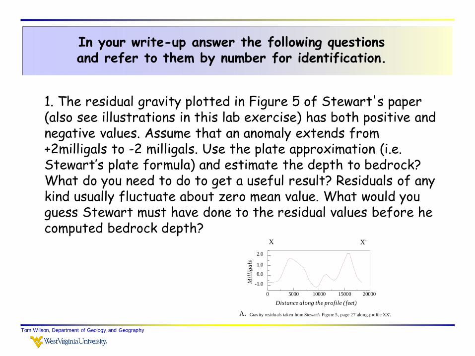
1. The residual gravity plotted in Figure 5 of Stewart's paper (also see illustrations in this lab exercise) has both positive and negative values. Assume that an anomaly extends from +2milligals to -2 milligals. Use the plate approximation (i.e. Stewart’s plate formula) and estimate the depth to bedrock? What do you need to do to get a useful result? Residuals of any kind usually fluctuate about zero mean value. What would you guess Stewart must have done to the residual values before he computed bedrock depth?

In your write-up answer the following questions and refer to them by number for identification.

?

X

A.

B.

Gravity residuals taken from Stewart's Figure 5, page 27 along profile XX'.

Depth model is simplified from that presented by Stewart (Figure 5, page 27).

X X'

-1.0

0.0

1.0

2.0M

illi

ga

ls

0 5000 10000 15000 20000

Distance along the profile ( feet)

X'

0 5000 10000 15000 20000

Distance along profile ( feet)

0

200

400

600Dep

th (

feet

)


2. At the beginning of the lab you made a copy of GMSYS window showing some disagreement between the observations (dots) and calculations (solid line) across Stewart's model (section XX' Figure 7). As we did in class and in the lab manual, note a couple areas along the profile where this disagreement is most pronounced, label these areas in your figure for reference. In your lab report discussion offer an explanation for the cause(s) of these differences? Assume that the differences are of geological origin and not related to errors in the data.


See lab

manual


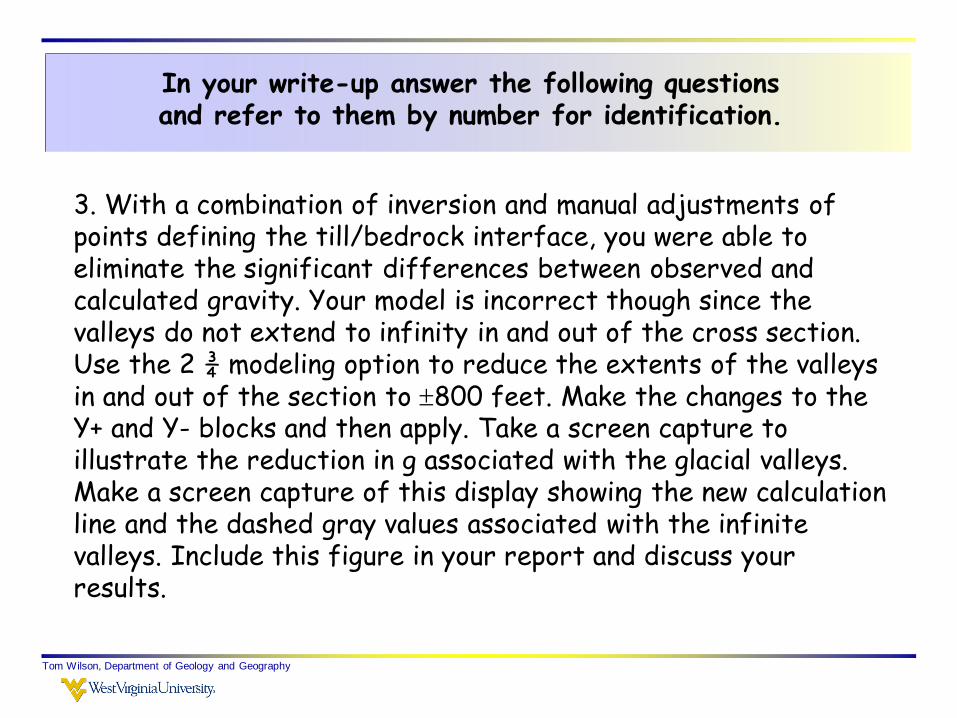
3. With a combination of inversion and manual adjustments of points defining the till/bedrock interface, you were able to eliminate the significant differences between observed and calculated gravity. Your model is incorrect though since the valleys do not extend to infinity in and out of the cross section. Use the 2 ¾ modeling option to reduce the extents of the valleys in and out of the section to 800 feet. Make the changes to the Y+ and Y- blocks and then apply. Take a screen capture to illustrate the reduction in g associated with the glacial valleys. Make a screen capture of this display showing the new calculation line and the dashed gray values associated with the infinite valleys. Include this figure in your report and discuss your results.


Note differences between infinitely long valleys and

those extending in and out of the section only 0.1 km.



4. Use Stewart's formula t = 130g and estimate the depth to bedrock at the x location of 7920 feet along the profile. Does it provide a reliable estimate of bedrock depth in this area? Explain in your discussion.

5. Lastly, describe the model you obtained and comment on how it varies from the starting model taken from Stewart.


Remember that Stewart assumes a negative density

contrast so all anomalies must be negative


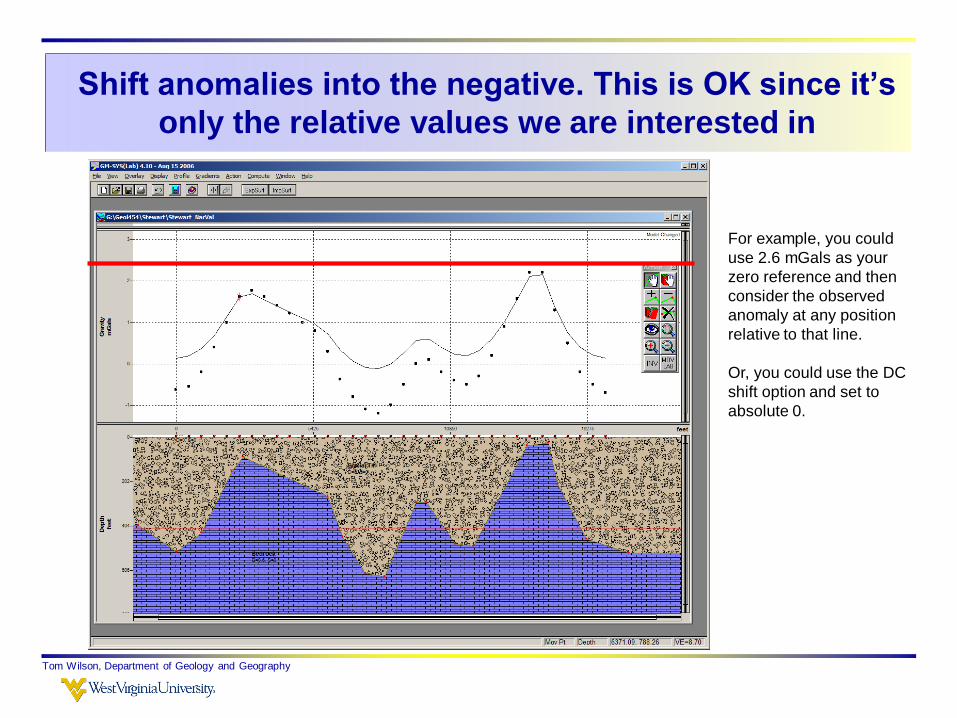
Shift anomalies into the negative. This is OK since it’s

only the relative values we are interested in


For example, you could

use 2.6 mGals as your

zero reference and then

consider the observed

anomaly at any position

relative to that line.

Or, you could use the DC

shift option and set to

absolute 0.

Use questions to guide your discussion


The questions in the lab guide provide discussion points for your lab report. Use figures you've generated in GMSYS to illustrate your point. All figures should be numbered, labeled and captioned.

In class problem


Gravity Lab & Intro Problems Review - West Virginia...

Documents

Transcript of Gravity Lab & Intro Problems Review - West Virginia...