Variability – Waiting Times Sources: Matching Supply with Demand, 3e, Cachon/Terwiesch.

Slide 1In search of the bullwhip effect: Cachon, Randall, Schmidt 9/06
In search of the bullwhip effect
Gérard P. CachonThe Wharton School
University of Pennsylvania
PresentedSeptember 9, 2006
Northwestern University
Glen M. SchmidtMcDonough School of Business
Georgetown University
Taylor RandallDavid Eccles School of Business
University of Utah

Slide 2In search of the bullwhip effect: Cachon, Randall, Schmidt 9/06
The bullwhip effect
Demand variability increases as you move up the supply chain from the customer towards supply
CustomerRetailerDistributorFactoryTier 1 SupplierEquipment
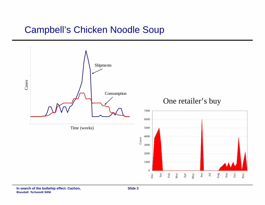
Slide 3In search of the bullwhip effect: Cachon, Randall, Schmidt 9/06
Campbell’s Chicken Noodle Soup
Time (weeks)
Cas
es
Shipments
Consumption
0
1000
2000
3000
4000
5000
6000
7000
Dec Ja
n
Feb
Mar
Apr
May Ju
n
Jul
Aug Se
p
Oct
Nov
Cas
es
One retailer’s buy
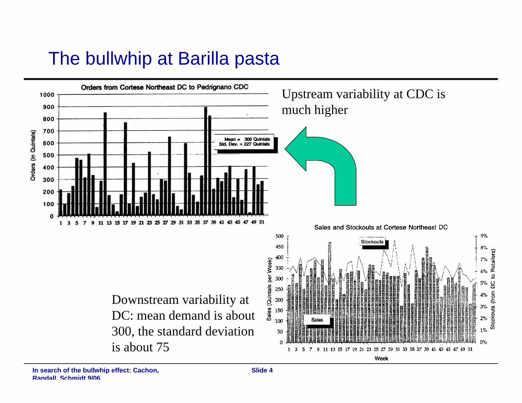
Slide 4In search of the bullwhip effect: Cachon, Randall, Schmidt 9/06
The bullwhip at Barilla pasta
Downstream variability at DC: mean demand is about 300, the standard deviation is about 75
Upstream variability at CDC is much higher

Slide 5In search of the bullwhip effect: Cachon, Randall, Schmidt 9/06

Slide 6In search of the bullwhip effect: Cachon, Randall, Schmidt 9/06
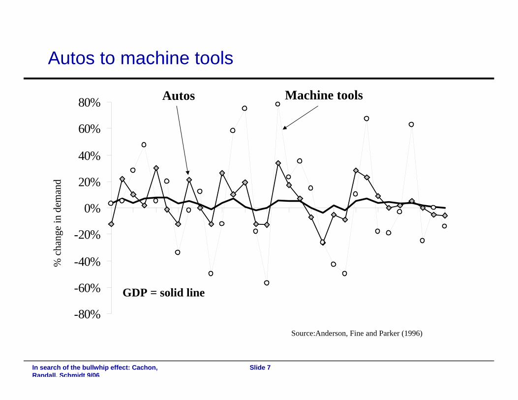
Slide 7In search of the bullwhip effect: Cachon, Randall, Schmidt 9/06
Autos to machine tools
-80%
-60%
-40%
-20%
0%
20%
40%
60%
80%
% c
hang
e in
dem
and
GDP = solid line
Source:Anderson, Fine and Parker (1996)
Autos Machine tools
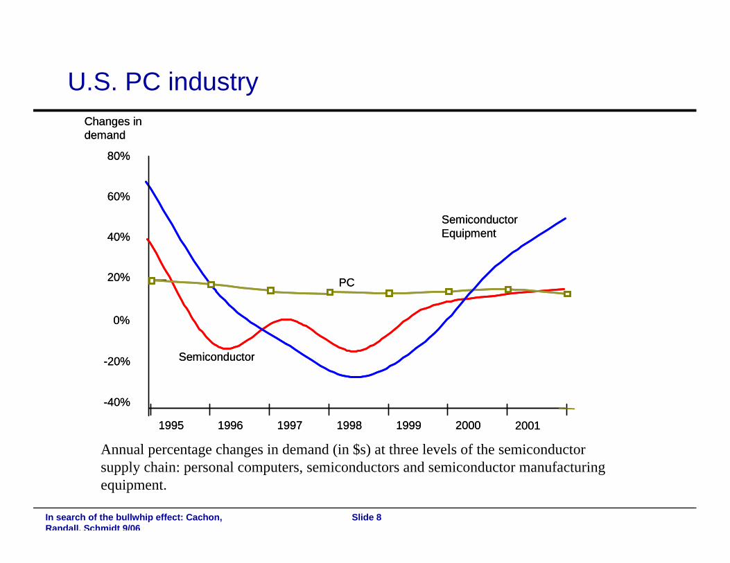
Slide 8In search of the bullwhip effect: Cachon, Randall, Schmidt 9/06
U.S. PC industry
Semiconductor
1995 1996 1997 1998 1999 2000 2001
-40%
-20%
0%
20%
40%
60%
80%
PC
SemiconductorEquipment
Changes indemand
Semiconductor
1995 1996 1997 1998 1999 2000 2001
-40%
-20%
0%
20%
40%
60%
80%
PC
SemiconductorEquipment
Changes indemand
Annual percentage changes in demand (in $s) at three levels of the semiconductor supply chain: personal computers, semiconductors and semiconductor manufacturing equipment.

Slide 9In search of the bullwhip effect: Cachon, Randall, Schmidt 9/06
Explanations for the bullwhip effect …
Fixed cost to produce/order, (s,S) models, order synchronization: Blinder (1981), Caplin (1985), Caballero and Engel (1999), Mosser (1991), Lee, Padmanabhan and Whang (LPW) (1997), Cachon (1999)
Positive serial correlation of demand shocks: Kahn (1987), LPW (1997), Graves (1999), Chen, Drezner, Ryan, Simchi-Levi (2000).
Price fluctuations/cost shocks: LPW (1997)
Non-convex production: Ramey (1991)
Demand can be backlogged: Kahn (1987)
Shortage gaming: LPW (1997), Cachon and Lariviere (1997)
Misperception of feedback/irrational behavior: Sterman (1989)

Slide 10In search of the bullwhip effect: Cachon, Randall, Schmidt 9/06
Empirical evidence of production smoothing
Blinder and Maccini (91,92):⎯ Data: 1959-1986, monthly, seasonally adjusted, constant 1982 dollars⎯ Production is more variable than sales in 17 of 20 two-digit manufacturing industries⎯ “… the basic facts to be explained are … 1) production is more variable than sales in most
industries”.
Blanchard (1983):⎯ “… in the automobile industry, inventory behavior is destabilizing: the variance of production
is larger than the variance of sales.”
Miron and Zeldes (1988):⎯ “…The overall assessment of this model … is quite negative: there is little evidence that
manufacturers hold inventories of finished goods … to smooth production.”
Eichenbaum (1989):⎯ “We find overwhelming evidence against the production-level smoothing model … we
conclude that the variance of production exceeds the variance of sales in most manufacturing industries.”
Other negative results:⎯ West (1986), Ramey (1991), Mosser (1991), Kahn (1992)
Slide 11In search of the bullwhip effect: Cachon, Randall, Schmidt 9/06
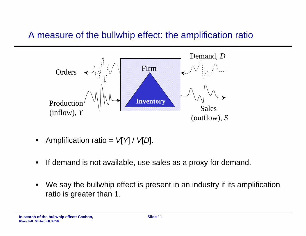
A measure of the bullwhip effect: the amplification ratio
Amplification ratio = V[Y] / V[D].
If demand is not available, use sales as a proxy for demand.
We say the bullwhip effect is present in an industry if its amplification ratio is greater than 1.
Demand, D
Inventory
Firm
Sales(outflow), S
Orders
Production(inflow), Y

Slide 12In search of the bullwhip effect: Cachon, Randall, Schmidt 9/06
Our data
Sources: ⎯ Census Department, Bureau of Economic Analysis.
Data:⎯ U.S., 1992-2006, monthly.⎯ 50 manufacturing industries: Sales, inventory.
• In a subset of 23 manufacturing industries: Demand.⎯ 16 wholesale industries: Sales, inventory.⎯ 6 retail industries: Sales, inventory.
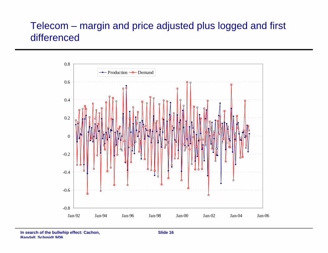
Data manipulations: 1) Adjust Demand and Sales series for margins and price.2) Adjust Inventory series for price.3) For each industry evaluate a Production series: Yt = St + ∆ It4) Log and first difference the Production, Demand and Sales series.

Slide 13In search of the bullwhip effect: Cachon, Randall, Schmidt 9/06
General merchandise stores – margin and price adjusted
10,000
15,000
20,000
25,000
30,000
35,000
40,000
45,000
50,000
55,000
Jan-92 Jan-94 Jan-96 Jan-98 Jan-00 Jan-02 Jan-04 Jan-06
Production Sales

Slide 14In search of the bullwhip effect: Cachon, Randall, Schmidt 9/06
General merchandise stores – margin and price adjusted plus logged and first differenced
-1
-0.8
-0.6
-0.4
-0.2
0
0.2
0.4
0.6
Jan-92 Jan-94 Jan-96 Jan-98 Jan-00 Jan-02 Jan-04 Jan-06
Production Sales
Slide 15In search of the bullwhip effect: Cachon, Randall, Schmidt 9/06
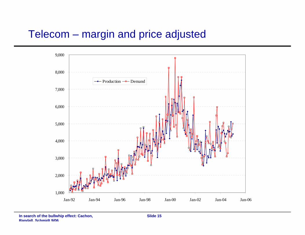
Telecom – margin and price adjusted
1,000
2,000
3,000
4,000
5,000
6,000
7,000
8,000
9,000
Jan-92 Jan-94 Jan-96 Jan-98 Jan-00 Jan-02 Jan-04 Jan-06
Production Demand
Slide 16In search of the bullwhip effect: Cachon, Randall, Schmidt 9/06
Telecom – margin and price adjusted plus logged and first differenced
-0.8
-0.6
-0.4
-0.2
0
0.2
0.4
0.6
0.8
Jan-92 Jan-94 Jan-96 Jan-98 Jan-00 Jan-02 Jan-04 Jan-06
Production Demand
c
Slide 17In search of the bullwhip effect: Cachon, Randall, Schmidt 9/06
Research questions
To what extent does the bullwhip effect exist in U.S. industry level data?⎯ Are amplification ratios greater than 1?⎯ Do manufacturers experience the highest demand variability and
retailers the lowest?
Understand variation in the amplification ratios:⎯ What explains variation in the amplification ratio across industries?⎯ Have amplification ratios been decreasing over time?

Slide 18In search of the bullwhip effect: Cachon, Randall, Schmidt 9/06
Prevalence of the bullwhip effect
Aggregate series Amplification RatioRetail 0.50Wholesale 1.14Manufacturing 0.55
Seasonally unadjusted
Seasonally adjusted
Retail 16% (1 of 6) 100% (6 of 6)Wholesale 88% (14 of 16) 100% (16 of 16)Manufacturing 40% (20 of 50) 74% (37 of 50)
Percentage of industries that exhibit the bullwhip effect
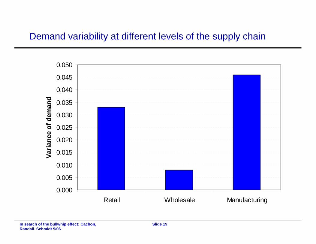
Slide 19In search of the bullwhip effect: Cachon, Randall, Schmidt 9/06
Demand variability at different levels of the supply chain
0.000
0.005
0.010
0.015
0.020
0.025
0.030
0.035
0.040
0.045
0.050
Retail Wholesale Manufacturing
Varia
nce
of d
eman
d
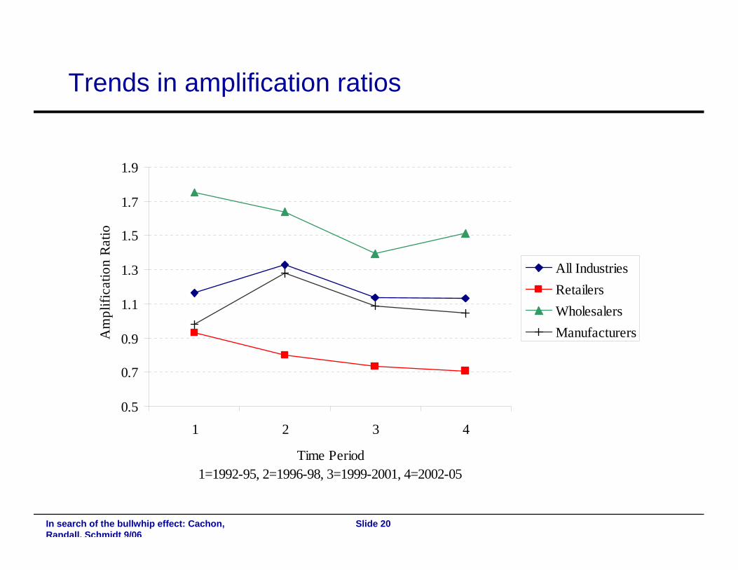
Slide 20In search of the bullwhip effect: Cachon, Randall, Schmidt 9/06
Trends in amplification ratios
0.5
0.7
0.9
1.1
1.3
1.5
1.7
1.9
1 2 3 4
Time Period1=1992-95, 2=1996-98, 3=1999-2001, 4=2002-05
Am
plifi
catio
n R
atio
All IndustriesRetailersWholesalersManufacturers
Slide 21In search of the bullwhip effect: Cachon, Randall, Schmidt 9/06
Future research
Investigate the bullwhip effect at different levels of aggregation –firm, category, sku.
Investigate the bullwhip effect at different levels of time aggregation – daily, weekly, quarterly.
Obtain better order and demand data.
Do firms/supply chains that better manage the bullwhip effect perform better financially?