Graph Matrices and Applications

Graph Matrices and Applications

Note: Please use a slide show since transitions have been animated. Tip: dark red text corresponds to dark red entries in the table for that slide and so on . . .

Overview:

Graph matrices are just another representation for graphs

• We will be covering - the need for matricesMatrix operations, relations node reduction algorithm equivalence class partition

Why do we need matrices?…• Path tracing can lead to errors• Links can be missed or covered twice

(redundancy)• Interruptions while tracing a path can cause

errors and lead to confusion• There is a need for a more methodical and

mechanical approach• Proving theorems by mathematical

representations(matrices) helps in proving theorems about graphs

Operations that comprise the toolkit…• Matrix multiplication, which is used to get the

path expression from every node to every other node

• A partitioning algorithm for converting graphs with loops into loop free graphs of equivalence classes

• A collapsing process (analogous to the determinant of a matrix) which gets the path expression from any node to any other node

The matrix of a graph

• A graph matrix is a square array with one row and one column for every node of the graph

• Each row-column combination corresponds to a relation b/w the node corresponding the row and the node corresponding the column. This could be the link name.

0 GRAPH MATRIX

1

Graph matrix observations:

• The size of the matrix (i.e. the number of rows and columns) equals the number of nodes

GRAPH a 0 MATRIX

• If there are several links between two nodes, then, the entry is a sum. The ‘+’ sign denotes parallel links, as usual.

a

GRAPH b MATRIX

1

1 2 a + b

Graph matrix observations (cont…)

• The entry at a row and column intersection is the link weight of the link (if any) that connects the two nodes in that direction

a

e b d c

GRAPH MATRIX

1 2

3

a d

b+e

c

Graph matrix observations (cont…)

• A connection from node i to node j does not imply(mean) a connection from node j to node i as seen in the graph.

• There is a place to put every possible direct connection or link between any node and any other node.

a

GRAPH b MATRIX

1 2 a b

Definitions:• The simplest weight that we can denote is to

indicate if there is a connection or not. Say – ‘1’ means that there is a connection and ‘0’ means that there is no connection. The arithmetic rules as we already know are-

1 + 1 = 1 1 + 0 = 1 0 + 0 = 0 1 * 1 = 1 1 * 0 = 0 0 * 0 = 0 A matrix with weights defined is called a

connection matrix.

Obtaining the connection matrix-• Replace each entry with ‘1’ if there is a link and with ‘0’ if

there isn’t. To reduce clutter, ignore the ‘0’s.• Each row of the matrix denotes the out-link of the node

corresponding to that row• Each column denotes the in-link corresponding to that node• A branch node has more than one non-zero entry in its row• A junction node has more than one non-zero entry in its

column• A Self loop is an entry along the diagonal• Graph’s cyclo-matic complexity (will be dealt further)

Deducing the relation matrix…

a b c h g m d e f l i j k

1 5 6 7 8

3

4

2

a i

b h

j

m

c l d

e

f k g

RELATION MATRIX

Replace each entry with the link weight if there is a link and leave it blank if there isn’t.

Deducing the connection matrix & calculating the cyclomatic complexity…

a b c h g m d e f l i j k

1 5 6 7 8

3

4

2

1 1

1 1

1

1

1 1 1

1

1 1 1

CONNECTION MATRIX

2 - 1 = 1

2 - 1 = 1

1 - 1 = 0

1 - 1 = 0

3 - 1 = 2

1 - 1 = 0

3 - 1 = 2

Cyclo-matic complexity

6 + 1 = 7 = M

Replace each entry with ‘1’ if there is a link and leave it blank if there isn’t.

Add the entries in each row & subtract the total by 1.

Now add the results from each row. You get 6.Adding 1 to this gives you the cyclo-matic complexity (M).

Simplifying references- • Instead of saying- ‘entry at row 6, column 7’, we say

– entry at node i and column j.• So, the link weight between nodes i and j is

represented by aij

• Self loop at node i is represented by aii

• So, the link weight between nodes j and i is

represented by aji

b c

a m d

1 5 6

3

7

w.r.t the graph,

abmd should read a13 a35 a56 a67

where, a13 = a

a35 = b…

Examples-

• aij ajj ajm This expression denotes a path from node i to j, with a self loop at j and then a link from node j to m.

• ∑aik akk akj (where k = 1 to n) This expression denotes the set of all possible paths between nodes i and j via one(or many) intermediate node(s).

Definitions:• The transpose of a matrix is the matrix with rows and columns

interchanged (denoted by superscript T) . If C = AT , then cij = aji • The intersection of two matrices of the same size, (denoted by

A # B) is obtained by an element-by-element multiplication of

the entries. C = A # B cij = aji (usually Boolean AND/ set intersection)

• The union of two matrices is defined as the element-by-element addition (usually Boolean OR/ set union).

Relations:• A relation is a property that exists between two objects of

interest.a and b are objects and R is used to denote that a has a relation to b.

Examples:aR b a is connected to b. R = ‘is connected to’a>= b or aR b R is ‘is greater that or equal to’A is a subset of b R is ‘is a subset of’

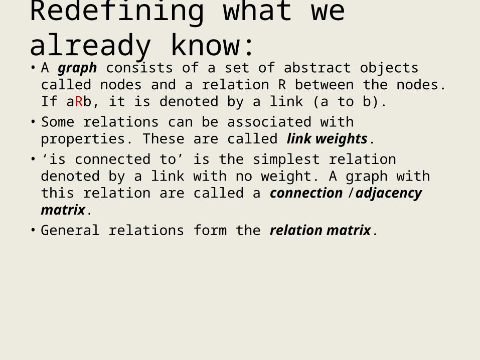
Redefining what we already know:• A graph consists of a set of abstract objects called nodes

and a relation R between the nodes. If aRb, it is denoted by a link (a to b).

• Some relations can be associated with properties. These are called link weights.

• ‘is connected to’ is the simplest relation denoted by a link with no weight. A graph with this relation are called a connection /adjacency matrix.

• General relations form the relation matrix.

Properties of relations (overview):• Transitive relations

a R b b R c a R c • Reflexive relations

for every a, a R a (eg. self loop)• Symmetric relations (undirected graph)

for every a & b, a R b b R a (aij = aji for all i, j) • Anti-symmetric relations

for every a & b, a R b b R a, then a = b• Equivalence relations

satisfies transitive, reflexive & symmetric• Partial ordering relations

satisfies transitive, reflexive & anti-symmetric

Properties of relations:• Transitive relations

a R b b R c a R c Most relations used in testing are transitive.Examples for transitive relations: is connected

to, is greater than or equal to, is less than or equal to, is a relative of, is faster than, is slower than, takes more time than, is a subset of, includes, shadows, is the boss of.

Examples for intransitive relations: is acquainted with, is a friend of, is a neighbor of, is lied to, has a du chain between.

Properties of relations (cont…):• Reflexive relations

for every a, a R a (eg. self loop) A reflexive relation is equivalent to a self loop

at every node.Examples for reflexive relations: equals, is

acquainted with, is a relative of.Examples for ir-reflexive relations: not equals, is

a friend of(unfortunately), is on top of, is under.

Properties of relations (cont…):• Symmetric relations (undirected graph)

for every a & b, a R b b R a (aij = aji for all i, j) This implies that if there is a link from a to b, there is

also a link from b to a. Which means that instead of two way links between nodes we can just have a single undirected link . A graph whose relations are not symmetric is called a directed graph.

Examples for symmetric relations: is a relative of, equals, is alongside of, shares a room with, is married, brother of, OR, AND, XOR.

Examples for asymmetric relations: is the boss of, is the husband of, is greater than, controls, dominates, can be reached from.

Since we need to use arrows to

denote direction

Properties of relations (cont…):• Anti-symmetric relations

for every a & b, a R b b R a, then a = bThis implies that both a & b are the sameelements.Examples for anti-symmetric relations: is greater than or

equal to, is a subset of, time.Examples for non-antisymmetric relations: is connected

to, can be reached from, is greater than, is a relative of, is a friend of.

Properties of relations (cont…):• Equivalence relations

satisfies transitive, reflexive & symmetricExample for equivalence relations: numerical equality.• If a set of objects satisfy an equivalence relation, they

form an equivalence class over that relation. • Importance of equivalence classes & relations:

any member of the equivalence class, is with respect to the relation , equivalent to any other member of the class. [Please refer the text for short notes]

Properties of relations (cont…):• Partial ordering relations

satisfies transitive, reflexive & anti-symmetricProperties: loop free, there is at least 1 maximum element & one minimum element,

if you reverse all the rows, the resulting graph is also partially ordered.Example for partial ordering relations: trees, most data structures, integration plan.• A maximum element a, is one for which the relation xRa does not hold for any

other element x.• A minimum element a, is one for which the relation aRx does not hold for any

other element x. [Please refer the text for short notes]

Partitioning algorithm:

8

2 7

1

6

4

3

5

1 1

1 1 1

1 1

1 1 1

1 1

1

1 1 1

1 1

RELATION MATRIX

… Considering that the graph may have loops. Diagonal entries are made to represent self loop.

Partitioning algorithm(cont…):

8

2 7

1

6

4

3

5

1 1 1 1 1 1 1

1 1 1 1 1 1

1 1 1 1

1 1 1 1

1 1 1 1

1

1 1 1 1 1 1

1 1 1 1 1

TRANSITIVE CLOSURE MATRIX… Explanation for getting the transitive closure matrix & its transpose is not included since we assumed that you would know this. Please get back if you need any

info.


8

2 7

1

6

4

3

5

1

1 1

1 1 1

1 1 1

1 1 1

1

1 1

1

INTERSECTION WITH ITS TRANSPOSE

A = [ 1 ]B = [ 2, 7 ]C = [ 3, 4, 5 ]D = [ 6 ]E = [ 8 ]

Considering the entries is the above matrix, we have the following…

Example: to get values for B – It is evident that B(row 2) has entries at column 2 & 7. Hence the values.


8E

2,7B

1A

6D

3,4,5 C

1 1

1 1

1 1

1

1 1

The resulting graph is ---

A B C D E A

B

C

D

E

From the earlier slide,we had --A = [ 1 ]B = [ 2, 7 ]C = [ 3, 4, 5 ]D = [ 6 ]E = [ 8 ]

… Considering that the graph had self loops. Diagonal entries are made to represent self loop.

Node Reduction Algorithm – some matrix properties:

a

d b

c f

g e h

a

c f

d b

g e h

a

c f

d b

g e h

1 2

3

4

5

1 2 3 4 5

To interchange node names in a matrix, we must interchange both the corresponding rows and the corresponding columns…

1 2

4

3

5

1 2

*

*

5

1 2 * * 5

1 2 4 3 5

interchanging rows 3 & 4 …

interchanging columns 3 & 4 …

*Node Reduction Algorithm*• Advantages:

– The matrix reduction method is more methodical than the graphical method– Does not entail(involve) continually redrawing of the graph

• Steps to be followed:– Select a node for removal, replace the node by equivalent links that bypass that

node.– Add the parallel terms & simplify if you can– Adjust out-links that have a self loop– The result is a matrix whose size is reduced by 1. – Continue until only two nodes are left. There should be only one link between

these nodes.

*Node Reduction Algorithm* d

a b c e f g

h

1 3 4 2

5a

d b

c f

g e h

1 2

3

4

5

1 2 3 4 5

STEP 1: Eliminate a node and replace it with a set of equivalent links…

Say, we start with eliminating node 5-

TIP: The out-link of the node removed will correspond to the row and the in-link will correspond to the column

*Node Reduction Algorithm*

d

a b c e f g

h

1 3 4 2

5

a

d b

c f

g e h

1 2

3

4

5

1 2 3 4 5

Say, we start with eliminating node 5. First, we remove the self loop-

Eliminating node 5 … the self loop is represented with a * and the outgoing link from the node is multiplied . . .

h*g h*e



d

a b c + fh*e (fh*g)

1 3 4 2

a

d b

c f

g e h

1 2

3

4

5

1 2 3 4 5

Now, we eliminate node 5-

Eliminating node 5 … the self loop is represented with a * and the outgoing link from the node is multiplied . . .

h*g h*e

C+fh*g fh*e



d

a b fh*e c + (fh*g)

1 3 4 2

a

d b

c f

g e h

1 2

3

4

5

1 2 3 4 5

Now, we eliminate node 4-

Eliminating node 4 … the parallel link is added up and serial links multiplied . . .

h*g h*e

C+fh*g fh*e

bfh*e bc + b(fh*g)

d+bc+bfh*g bfh*g

d +


a

1 3 2

a

d b

c f

g e h

1 2

3

4

5

1 2 3 4 5Now, we should ideally eliminate node 3-Since row 2 and column 2 are empty, these are dropped. Values of nodes 1 and 3 are retained.

Eliminating node 4 … the parallel link is added up and serial links multiplied . . .

h*g h*e

C+fh*g fh*e

bfh*e bc + b(fh*g)

d+bc+bfh*g bfh*g

d + X

If row n and its corresponding column n is not empty, them we need to continue removing node 3 and retain values for nodes 1 & 2.

3

Building tools (node degree & graph density):• The out-degree of a node is the number of out-links it has.• The in-degree of a node is the number of in-links it has.• The degree of a node is the sum of in-degree and out-

degree.• The average degree(mean) of a node is b/w 3 and 4.• Degree of a simple branch/junction is 3• Degree of a loop contained in 1 statement is 4• Mean degree of 4 or 5 very busy flow graph

Node Reduction Optimization (tips):• The optimum order for node reduction is to do the lowest degree

nodes first.• When a node with degree 3(may be 1 in-link & 2out-links or 2 in-links

& 1 out-link) is removed , it reduces the total link count by 1 link.• A degree 4 node keeps the link count the same & all higher degree

nodes increase the link count.

What’s wrong with arrays?Matrix as a 2-dimensional array is notconvenient for larger graphs. Herez why!...We have four reasons for the same-• Space: For a matrix representation of an array, space

grows as n2 whereas, for a linked list, it grows only as kn, where k is a small number such as 3 or 4.

• Weights: Most weights in arrays are complicated and may have many components. This means that an additional weight matrix is required for each such weight.

What’s wrong with arrays? (cont…)• Variable-length weights: If the weights are regular

expressions/algebraic expressions, we would then need a 2-dimensional string array (most of whose entries would be null).

• Processing time: Even though operations over null entries are fast, it still takes time to access such entries and discard them.The matrix representation forces us to spend a lot of time processing combinations of entries that we know will yield null results.

Building tools - Linked list representations: d a b c

e f g h

1 3 4 2

5

a

d b

c f

g e h

1 2 3 4 51 2

3

4

5 node1, 3 ; a

node1,2,

node3, 2 ; d

node3, 4; b

node4, 2 ; c

node4, 5 ; f

node5, 2 ; g

node5, 3 ; e

node5, 5 ; h

Every node is a unique name/ number. A link is a pair of node names.The linked list entries for the above are …

The link names will usually be pointers to entries in a string array(where actual weight expressions are stored).

If the weights are fixed length, they can be associated with links in parallel-fixed entry length array.

Format for linked list entries:row, column ; data entry

Building tools - Linked list representations:

1, 3 ; a

2,

3, 2 ; d

3, 4; b

4, 2 ; c

4, 5 ; f

5, 2 ; g

5, 3 ; e

5, 5 ; h

Clarifying entries by using node names & pointers…

Fig.1 is represented in a more logical format in Fig.2 by representing the nodes under list entry. Fig 3 is more detailed the with in-links to that node added (highlighted in black).

list entry content

1 node1, 3 ; a

2 node2,exit

3 node3, 2 ; d

3, 4; b

4 node4, 2 ; c

4, 5 ; f

5 node5, 2 ; g

5, 3 ; e

5, 5 ; h

list entry content1 node1, 3 ; a

2 node2,exit

3,

4,

5,

3 node3, 2 ; d

3, 4; b

1,

5,

4 node4, 2 ; c

4, 5 ; f

3,

5 node5, 2 ; g

3 ; e

5 ; h

4,

5,

Matrix operations:• Parallel Reduction: the easiest operation. After

sorting, parallel links are adjacent entries with the same pair of node names.

Example: Say we have 3 parallel links from node 17 to node 44. y, z & w are the pointers to the weight expressions.

node 17, 21 ; x

, 44 ; y

, 44 ; z

, 44 ; w

Depicting all the entries for parallel links between node 17 & node 44, we have -

node 17, 21 ; x

, 44 ; y

where, y = y + z + w

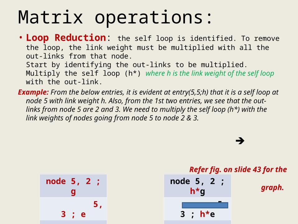
Matrix operations:• Loop Reduction: the self loop is identified. To remove the loop,

the link weight must be multiplied with all the out-links from that node. Start by identifying the out-links to be multiplied. Multiply the self loop (h*) where h is the link weight of the self loop with the out-link.

Example: From the below entries, it is evident at entry(5,5;h) that it is a self loop at node 5 with link weight h. Also, from the 1st two entries, we see that the out-links from node 5 are 2 and 3. We need to multiply the self loop (h*) with the link weights of nodes going from node 5 to node 2 & 3.

node 5, 2 ; g

5, 3 ; e

5, 5 ; h

node 5, 2 ; h*g

5, 3 ; h*e

5, 5 ; h

Refer fig. on slide 43 for the graph.

Matrix operations:• Cross-Term Reduction: Select a node for reduction. The

cross-term step requires that you combine every in-link to the node with every out-link from that node. The in-links are obtained by back pointers. The new links created be removing the node will be associated with the nodes of the in-links. Example: Say that the node to be removed was node 4.

• d• b c f

• d bc

• bf

list entry content

2 node2, exit

(inlink)4, 2

(inlink)3,2

3 node3,2 ; d

3,4 ; b

4 node4, 2 ; c

4, 5 ; f

(inlink)3,4; b

5 (inlink)4, 5

3 4 2

5

list entry content2 node2, exit

(inlink)4, 2

(inlink)3,2

3 node3,2 ; d

3,2 ; bc

3,5 ; bf4 node4, 2 ; c

4, 5 ; f

(inlink)3,4; b

5 (inlink) 4, 5

3 2

5

The changes are highlighted in dark red

The powers of a matrix has not been covered. This includes basic matrix multiplication that you already know & sets of paths.

Please read through… Page 405 of the

Boris Beizer text.

*** Some Questions picked up from the previous papers for units V, VI, VII, VIII ***--8 marks questions--1.Write the designers comments about state graphs. 2.Write an algorithm for all pair paths using matrix operations. 3.Define – maximum element and minimum element of a graph. 4.Explain parallel reduction and loop reduction. 5.Explain - a) Distributive laws b) Absorption rule6.Illustrate the applications of Decision tables? 7.The behavior of a finite state machine is invariant under all encodings. Justify? 8.What operations does a tool kit consist for the representation of graphs? 9.How can a relation matrix be represented and what are the properties of relations? 10.What are the rules of Boolean algebra? --12 marks questions --1.Define the purpose of KV charts. Describe the use of KV charts in logic based testing. 2.Define a state chart. Define the method used to distinguish good and bad state graphs. 3.Briefly discuss the following - a) matrix of a graph b) node reduction algorithms--16 marks questions--1.Draw a hard disk recovery system with a state graph and state table. 2.What is decision table and how is it useful in testing? Explain it with the help of an example. 3.Write short notes on - a) Transition bugs b) Dead statesc) State bugs d) Encoding bugs.4.Explain State graphs with implementation? 5.What is Decision table and how is a Decision table useful in testing? Explain with the help of an example? 6.Explain - a) finite state machine b)state graph inputs and outputs c) transitions and state tables

Done!!! Do feel free to get back incase you have any questions

Note: Please read through the text by ‘Boris Beizer’ atleast once. This PPT is just for your reference & for step by step understanding of the

processing.

And yeah!!! Plz solve all the questions that

appeared in previous papers!

Graph Matrices and Applications

Documents

Transcript of Graph Matrices and Applications