Graph Embeddings Motivated by Greedy Routing

zur Erlangung des akademischen Grades eines

Doktors der Naturwissenschaften

von der KIT-Fakultät für Informatikdes Karlsruher Instituts für Technologie (KIT)

genehmigte

Dissertation

von

Roman Prutkin

aus Ekaterinburg

Tag der mündlichen Prüfung: 29. November 2017Erster Gutachter: Prof. Dr. Dorothea WagnerZweiter Gutachter: Prof. Dr. Martin NöllenburgDritter Gutachter: Prof. Dr. Michael Kaufmann

Roman Prutkin: Graph Embeddings Motivated by Greedy Routing,© 21. Februar 2018

To my family

D A N K S A G U N G

Als Erstes möchte ich mich bei Dorothea Wagner bedanken für die Möglichkeit,an ihrem Lehrstuhl meiner Promotion nachzugehen. Ich weiß es sehr zu schätzen,dass ich ohne Zeitdruck und unter äußerst komfortablen RahmenbedingungenForschungsfragen untersuchen konnte, die mich interessieren. Bei der Wahl derForschungsthemen war ich immer frei und bekam von Dorothea stets Rat undUnterstützung.

Michael Kaufmann danke ich, dass er sich bereit erklärt hat, meine Disserta-tion zu begutachten, sowie für seine Flexibilität bei der Terminfindung für diePromotionsprüfung.

Martin Nöllenburg und Ignaz Rutter haben mich sowohl bei meiner Diplom-arbeit als auch während meiner Promotion hervorragend betreut. Ich bin sehrfroh, dass ich von eurem Fachwissen und Erfahrung profitieren und von euchviel lernen konnte. Die Zusammenarbeit mit euch hat mir Spaß gemacht.

Ich bedanke mich bei meinen Koautoren Therese Biedl, Thomas Bläsius, XiaojiChen, Carsten Dachsbacher, Fabian Fuchs, Alexander E. Holroyd, Anton Kapla-nyan, Boris Klemz, Bongshin Lee, Moritz von Looz, Henning Meyerhenke, LevNachmanson, Benjamin Niedermann, Martin Nöllenburg, Nathalie Henry Richeund Ignaz Rutter.

Bei meinen aktuellen und ehemaligen Kollegen Lukas Barth, Moritz Baum, Tho-mas Bläsius, Guido Brückner, Valentin Buchhold, Julian Dibbelt, Fabian Fuchs,Andreas Gemsa, Sascha Gritzbach, Michael Hamann, Tanja Hartmann, AndreaKappes, Tamara Mchedlidze, Benjamin Niedermann, Martin Nöllenburg, ThomasPajor, Marcel Radermacher, Ignaz Rutter, Ben Strasser, Markus Völker, FranziskaWegner, Matthias Wolf, Tim Zeitz und Tobias Zündorf bedanke ich mich für dieangenehme und lockere Atmosphäre am Institut und die vielen Tischfußballspie-le, Kino-, Bastel- und Spieleabende, Wanderungen und Fußball-Sessions im SoccerCenter. Besonderer Dank geht an Fabian Fuchs, der mit mir das Sensornetze-Bürogeteilt hat.

Ich danke meiner Frau Anna, meinen Eltern Olga und Ilya und dem Rest mei-ner Familie für eure Inspiration und grenzenlose Unterstützung während meinerZeit als Doktorand, insbesondere in der Zeit des Schreibens dieser Arbeit.

v

D E U T S C H E Z U S A M M E N FA S S U N G

In dieser Arbeit untersuche ich Probleme aus Algorithmischer Geometrie undGraphentheorie, die Greedy Routing betreffen. Ich konzentriere mich insbesonde-re auf Greedy Routing in geometrisch eingebetteten Graphen, welches wie folgtdefiniert ist. Gegeben sei ein Graph G = (V, E), dessen Knoten V Koordinatenzugeordnet wurden, beispielsweise Punkte in der euklidischen Ebene. Kanten Esymbolisieren die Möglichkeit der direkten bidirektionalen Kommunikation zwi-schen Knoten. Jeder Knoten kennt seine eigenen Koordinaten und die seiner direk-ten Nachbarn in G. Beim Routing von Nachrichten in diesem Netzwerk nehmenwir zusätzlich an, dass jede Nachricht die Koordinaten des Ziels enthält.

s2

t2

s1 t1

Abbildung 1: Greedy Routingist erfolgreich zwischen demStart s1 und Ziel t1 (roter Pfad).Knoten s2 ist ein lokales Mini-mum für das Ziel t2.

Unter den obigen Annahmen ist die folgendeeinfache Routing-Strategie als Greedy Routing be-kannt. Für eine eingehende Nachricht berechnet je-der Knoten die euklidischen Distanzen zum Zielausgehend von sich selbst und von jedem seinerNachbarn und gibt anschließend die Nachricht aneinen Nachbarn weiter, der näher am Ziel liegt alsder Knoten selbst. Abbildung 1

.

zeigt einen geo-metrisch eingebetteten Graphen sowie einen mög-lichen Pfad beim Greedy Routing zwischen demStartknoten s1 und Ziel t1. Greedy Routing ist bei-spielsweise einer der beiden Routing-Modi im Pro-tokoll GPSR (Greedy Perimeter Stateless Routing) fürdrahtlose Sensornetze.

s2

t2

Abbildung 2: Eine Einbettungdes Graphen aus Abbildung 1

.

mit einer anderen Zuweisungder Knotenkoordinaten. Identi-sche Knoten haben die gleicheFarbe in beiden Abbildungen.Greedy Routing ist nun immererfolgreich.

Das Grundproblem von Greedy Routing ist,dass Nachrichten in lokalen Minima stecken blei-ben können, wo kein Nachbarknoten näher amZiel liegt (siehe zum Beispiel Abbildung 1

.

für denStartknoten s2 und Zielknoten t2).

Für einen gegebenen Graphen bestimmt dieWahl der Knotenkoordinaten die Erfolgsrate vonGreedy Routing. Für den Graphen in Abbildung 1

.

ist eine andere Koordinatenzuweisung in Abbil-dung 2

.

dargestellt. In der letzteren Einbettung istGreedy Routing von jedem Start- zu jedem Ziel-knoten erfolgreich. Grapheinbettungen mit die-ser Eigenschaft werden Greedy-Einbettungen bzw.Greedy-Zeichnungen genannt. Die Untersuchung

vii

der Greedy-Einbettungen wird in der Literatur durch Routing in drahtlosen Sen-sornetzwerken motiviert.

Senke

Abbildung 3: Sensornetze wer-den zur Erkennung von Wald-bränden verwendet.

Drahtlose Sensornetzwerke bzw. Sensornetze(engl. wireless sensor networks) sind Netzwerke vonkleinen mit Sensoren ausgestatteten Rechenkno-ten. Die Knoten sind räumlich verteilt und könnenuntereinander drahtlos kommunizieren. Obwohleinzelne Knoten typischerweise nur über begrenz-te Rechenkapazitäten sowie begrenzte Batterienverfügen, können die Knoten ein Netzwerk bil-den und eine Aufgabe in Zusammenarbeit erfül-len. Sie können beispielsweise Temperatur, Feuch-tigkeit, Konzentration von Kohlenmonoxid in der

Luft usw. überwachen und diese Daten an eine Basisstation weiterleiten als Teileines Systems, das Waldbrände erkennt und überwacht (siehe Abbildung 3

.

). Einsolches Netzwerk kann seine Aufgabe weiterführen, auch wenn einige Knotenausfallen. Anwendungsgebiete von Sensornetzen sind Militär, Umwelt, Gesund-heitswesen und Sicherheit.

Die Vision, wie man Greedy-Einbettungen für das Routing in Sensornetzenanwenden könnte, wird in der Literatur wie folgt geschildert. Das Sensornetz be-rechnet eine Greedy-Einbettung von seinem Kommunikationsgraphen und teiltjedem Knoten seine eigenen Koordinaten in dieser Einbettung mit (die sogenann-ten virtuellen Koordinaten) sowie die virtuellen Koordinaten der Nachbarknoten.Enthält nun jede Nachricht die virtuellen Koordinaten des Zielknotens, kann je-der Knoten die Kenntnis seiner virtuellen Koordinaten und der seiner Nachbarnnutzen, um die Nachricht mittels Greedy Routing weiterzuleiten. Da die virtuel-len Koordinaten aus einer Greedy-Einbettung stammen, ist Greedy Routing nunimmer erfolgreich. In dieser Arbeit untersuche ich die Realisierbarkeit dieser Visi-on aus dem Blickwinkel der Graphentheorie und erhalte neue Erkenntnisse überdie Frage, welche Graphen eine Greedy-Einbettung zulassen.

Abbildung 4: Eine Increasing-Chord-Graphzeichnung. Für je-den Start- und Zielknoten exis-tiert immer ein Pfad, entlangdessen Kanten die Distanz zumZiel kontinuierlich abnimmt.

Routing in Sensornetzen ist nicht die einzigeMotivation für die Untersuchung von Greedy-Einbettungen von Graphen und anderen verwand-ten Einbettungsarten. Kriterien wie etwa mög-lichst wenige lokale Minima spielen eine Rolle,wenn eine Netzwerkzeichnung Nutzern helfensoll, Pfade im Netzwerk zu finden. Dazu wurde inden letzten Jahren eine Reihe von verschiedenenZeichnungskonventionen vorgeschlagen, nämlichdie bereits erwähnten Greedy-Zeichnungen sowie(stark) monotone, Self-Approaching- und Increasing-Chord-Zeichnungen (siehe Abbildung 4

.

). Ich fasse das Problem, eine für die Pfad-suche geeignete Netzwerkeinbettung zu konstruieren, wie folgt auf: Finde füreinen gegebenen Graphen Knotenkoordinaten in R2, die verwendet werden kön-

viii

nen, um auf dem Graphen mit lokalen Entscheidungen zu routen, und sodassman Pfade finden kann, die immer Fortschritte in Richtung ihrer Ziele machen.Dies ist das zentrale Problem, das in dieser Arbeit untersucht wird.

überblick und beitrag

Ich betrachte mehrere Arten von Graphzeichnungen, die durch Greedy Routingauf geometrisch eingebetteten Graphen motiviert sind. Das zentrale Problem,das ich untersucht habe, ist, zu verstehen, welche Graphen eine Greedy-, Self-Approaching- oder Increasing-Chord-Zeichnung zulassen. Meine Arbeit erweitertden aktuellen Kenntnisstand zu dieser Frage um neue Erkenntnisse. Auf dem Wegzu einer vollständigen Charakterisierung von Graphen, die solche Zeichnungenzulassen, konzentriere ich mich auf gängige und wichtige Graphklassen wie Bäu-me, Triangulierungen und dreifach-zusammenhängende planare Graphen, die indiesem Forschungsbereich häufig betrachtet werden.

Außerdem untersuche ich die Komplexität des Problems, Polygone und Graph-zeichnungen in Teilbereiche zu zerlegen, die Greedy Routing unterstützen (sieheAbbildung 5

.

). Dieses Zerlegungsproblem entstammt direkt aus einem für drahtlo-se Sensornetzwerke vorgeschlagenen Routing-Algorithmus (Tan und Kermarrec,IEEE/ACM Trans. Networking 20.3 (2012

.

), 864–877) und ist stark verbunden mitIncreasing-Chord-Zeichnungen.

Euklidische Greedy-Zeichnungen von Bäumen

Im Zusammenhang mit dem Einbetten von Graphen in R2, um Greedy Routingzu unterstützen, ist folgendes Problem der „Heilige Gral“: Charakterisiere dieGraphen, die eine Greedy-Zeichnung in R2 besitzen. Dieses Problem zog großesInteresse der Graph-Drawing-Gemeinschaft auf sich. Obwohl die Existenz vonGreedy-Zeichnungen für mehrere Graphklassen gezeigt werden konnte, bleibt ei-ne vollständige Charakterisierung von Graphen, die eine Greedy-Zeichnung in R2

haben, ein bislang unerreichtes Ziel. Überraschenderweise blieb das Problem füreine solch natürliche Graphklasse wie Bäume offen. In dieser Arbeit charakteri-siere ich alle Bäume, die eine Greedy-Zeichnung in R2 besitzen. Dies beantworteteine Frage von Angelini et al. (Networks 59.3 (2012

.

), 267–274) und ist ein wichtigerSchritt in Richtung einer Charakterisierung der Greedy-einbettbaren Graphen.

Über Self-Approaching- und Increasing-Chord-Zeichnungen von dreifach-zusammenhän-genden planaren Graphen

Ich untersuche Self-Approaching- und Increasing-Chord-Zeichnungen für zweigängige Graphklassen: Triangulierungen und dreifach-zusammenhängende pla-nare Graphen. Ich zeige, dass in R2 alle Triangulierungen Increasing-Chord-Zeich-nungen besitzen und dass für planare 3-Bäume Planarität sichergestellt werdenkann. Außerdem beweise ich, dass binäre Kakteen, eine Graphklasse, die für die

ix

Konstruktion von Greedy-Zeichnungen von dreifach-zusammenhängenden pla-naren Graphen entscheidend war, nicht immer Self-Approaching-Zeichnungenhaben. Ich zeige, dass stark monotone (und damit Increasing-Chord-) Zeichnun-gen von Bäumen und binären Kakteen in manchen Fällen eine exponentielleAuflösung benötigen, und beantworte dadurch eine offene Frage von Kinder-mann et al. (Graph Drawing, 2014

.

, 488–500). Ich beweise, dass das Gleiche fürGreedy-Zeichnungen von binären Kakteen gilt. Ich zeige, dass dreifach-zusam-menhängende planare Graphen Increasing-Chord-Zeichnungen in der hyperboli-schen Ebene besitzen, und charakterisiere Bäume, die solche Zeichnungen haben.

Zerlegung von Graphzeichnungen und triangulierten einfachen Polygonen in Greedy-Routbare Regionen

s1

t2 pt1s2

Abbildung 5: Sei die Knotendichteinnerhalb der Netzwerkgrenze (grau)nah an unendlich. Greedy Routing lei-tet eine Nachricht entlang der geradenLinie zum Ziel weiter. Wird die Gren-ze getroffen, gleitet die Nachricht ent-lang der Grenze, solange es die Di-stanz zum Ziel verringert. Dies ist er-folgreich beim Routing von Punkt s1zu t1 (gestrichelte Bahn). Greedy Rou-ting von Punkt s2 zu t2 bleibt in einemlokalen Minimum p stecken. GreedyRouting innerhalb jeder der beidenPartitionen (hell- und dunkelgrau) istimmer erfolgreich.

Als nächstes betrachte ich Greedy Routingin kontinuierlichen Domänen und entdeckeeinen starken Zusammenhang zu Self-Ap-proaching- und Increasing-Chord-Zeichnun-gen von Graphen. Mehrere vorgeschlageneAnsätze für das Routing in drahtlosen Sen-sornetzwerken basieren auf der Idee, dasNetzwerk in Komponenten zu zerlegen, so-dass in jeder von ihnen Greedy Routing mitgroßer Wahrscheinlichkeit erfolgreich ist. Ei-ne globale Datenstruktur von vorzugsweisekleiner Größe speichert die Interkonnektivi-tät zwischen Komponenten.

Eine Greedy-Routbare Region (GRR) ist ei-ne abgeschlossene Teilmenge von R2, in derjeder beliebige Zielpunkt von jedem belie-bigen Startpunkt aus mit Greedy Routingerreicht werden kann (siehe Abbildung 5

.

).Tan und Kermarrec (IEEE/ACM Trans. Net-working 20.3 (2012

.

), 864–877) schlugen einen Routing-Algorithmus vor, der daraufbasiert, den Netzwerkbereich in wenige GRRs zu partitionieren. Sie zeigten, dasses NP-schwer ist, polygonale Regionen mit Löchern minimal zu zerlegen.

Ich untersuche minimale GRR-Zerlegung für planare geradlinige Zeichnungenvon Graphen, was eine natürliche Anpassung des GRR-Zerlegungsproblems fürPolygone darstellt. In diesem Kontext stimmen die GRRs mit Increasing-Chord-Zeichnungen von Bäumen überein. Ich zeige, dass die minimale Zerlegung immernoch NP-schwer für Graphen mit Zyklen und sogar für Bäume ist, aber für Bäumein Polynomialzeit optimal gelöst werden kann, wenn nur bestimmte Arten vonGRR-Kontakten zugelassen sind (z.B., wenn sich GRRs nicht kreuzen dürfen).Darüber hinaus gebe ich eine 2-Approximation für löcherfreie Polygone an fürden Fall, wenn eine gegebene Triangulierung eingehalten werden muss.

x

C O N T E N T S

1 introduction 1

.

2 related work 7

.

2.1 Routing in wireless ad hoc and sensor networks . . . . . . . . . . . . 7

.

2.1.1 Geographic routing . . . . . . . . . . . . . . . . . . . . . . . . . 8

.

2.2 Greedy embeddings . . . . . . . . . . . . . . . . . . . . . . . . . . . . 12

.

2.2.1 Graphs admitting Euclidean greedy embeddings . . . . . . . 12

.

2.2.2 Non-Euclidean greedy embeddings . . . . . . . . . . . . . . . 13

.

2.2.3 Succinctness . . . . . . . . . . . . . . . . . . . . . . . . . . . . . 13

.

2.3 Graph drawings with geodesic-path tendency . . . . . . . . . . . . . 14

.

2.3.1 Monotone drawings . . . . . . . . . . . . . . . . . . . . . . . . 14

.

2.3.2 Geometric spanners . . . . . . . . . . . . . . . . . . . . . . . . 16

.

2.3.3 Self-approaching and increasing-chord drawings . . . . . . . 16

.

2.4 Greedy geometric routing in continuous domains . . . . . . . . . . . 19

.

2.4.1 Beacon-based routing . . . . . . . . . . . . . . . . . . . . . . . 19

.

2.4.2 Network decomposition for routing . . . . . . . . . . . . . . . 20

.

3 preliminaries 23

.

3.1 Graphs, paths and connectivity . . . . . . . . . . . . . . . . . . . . . . 23

.

3.2 Graph drawings and polygons . . . . . . . . . . . . . . . . . . . . . . 24

.

3.2.1 Greedy, monotone, self-approaching and increasing-chorddrawings . . . . . . . . . . . . . . . . . . . . . . . . . . . . . . . 25

.

3.2.2 Used geometric notation . . . . . . . . . . . . . . . . . . . . . . 26

.

i graph embeddings motivated by greedy routing : existence 27

.

4 euclidean greedy drawings of trees 29

.

4.1 Introduction . . . . . . . . . . . . . . . . . . . . . . . . . . . . . . . . . 29

.

4.1.1 Contribution . . . . . . . . . . . . . . . . . . . . . . . . . . . . . 29

.

4.2 Preliminaries . . . . . . . . . . . . . . . . . . . . . . . . . . . . . . . . . 30

.

4.2.1 Example: independent stars . . . . . . . . . . . . . . . . . . . . 35

.

4.2.2 Outline of the characterization . . . . . . . . . . . . . . . . . . 36

.

4.2.3 Shrinking lemma . . . . . . . . . . . . . . . . . . . . . . . . . . 36

.

4.3 Opening angles of rooted trees . . . . . . . . . . . . . . . . . . . . . . 39

.

4.4 Arranging rooted subtrees with open angles . . . . . . . . . . . . . . 45

.

4.5 Characterizing greedy-drawable binary trees . . . . . . . . . . . . . . 53

.

4.6 Recognition algorithm . . . . . . . . . . . . . . . . . . . . . . . . . . . 56

.

4.6.1 Maximum degree 4 . . . . . . . . . . . . . . . . . . . . . . . . . 56

.

4.6.2 Maximum degree 5 and above . . . . . . . . . . . . . . . . . . 58

.

4.7 Conclusion . . . . . . . . . . . . . . . . . . . . . . . . . . . . . . . . . . 59

.

5 on self-approaching and increasing-chord drawings of 3-connected planar graphs 61

.

xi

xii contents

5.1 Introduction . . . . . . . . . . . . . . . . . . . . . . . . . . . . . . . . . 61

.

5.1.1 Contribution . . . . . . . . . . . . . . . . . . . . . . . . . . . . . 62

.

5.2 Preliminaries . . . . . . . . . . . . . . . . . . . . . . . . . . . . . . . . . 62

.

5.3 Graphs with self-approaching drawings . . . . . . . . . . . . . . . . . 65

.

5.3.1 Increasing-chord drawings of triangulations . . . . . . . . . . 65

.

5.3.2 Exponential worst case resolution . . . . . . . . . . . . . . . . 66

.

5.3.3 Non-triangulated cactuses . . . . . . . . . . . . . . . . . . . . . 73

.

5.4 Planar increasing-chord drawings of 3-trees . . . . . . . . . . . . . . . 79

.

5.5 Self-approaching drawings in the hyperbolic plane . . . . . . . . . . 81

.

5.6 Bounded dilation for Euclidean greedy drawings of cactuses . . . . . 84

.

5.7 Conclusion . . . . . . . . . . . . . . . . . . . . . . . . . . . . . . . . . . 86

.

ii greedy routing in continuous domains 89

.

6 partitioning into greedily routable regions 91

.

6.1 Introduction . . . . . . . . . . . . . . . . . . . . . . . . . . . . . . . . . 91

.

6.1.1 Contribution . . . . . . . . . . . . . . . . . . . . . . . . . . . . . 92

.

6.2 Preliminaries . . . . . . . . . . . . . . . . . . . . . . . . . . . . . . . . . 93

.

6.2.1 Greedily Routable Regions . . . . . . . . . . . . . . . . . . . . 93

.

6.2.2 Splitting graph drawings at non-vertices . . . . . . . . . . . . 97

.

6.2.3 Types of GRR contacts in plane straight-line graph drawings 98

.

6.3 NP-completeness for graphs with cycles . . . . . . . . . . . . . . . . . 99

.

6.4 Trees . . . . . . . . . . . . . . . . . . . . . . . . . . . . . . . . . . . . . 107

.

6.4.1 NP-completeness . . . . . . . . . . . . . . . . . . . . . . . . . . 108

.

6.4.2 Polynomial-time algorithms for restricted types of contacts . 112

.

6.5 Triangulations . . . . . . . . . . . . . . . . . . . . . . . . . . . . . . . . 124

.

6.6 Heuristics for simple polygons . . . . . . . . . . . . . . . . . . . . . . 126

.

6.7 Conclusion . . . . . . . . . . . . . . . . . . . . . . . . . . . . . . . . . . 127

.

7 conclusion 133

.

iii appendix 137

.

a appendix 139

.

bibliography 143

.

list of publications 157

.

1I N T R O D U C T I O N

In this thesis, I study problems from computational geometry and graph the-ory concerned with greedy routing. In particular, I focus on greedy routing ongeometrically embedded graphs, which is defined as follows. We are given agraph G = (V, E) whose nodes V have been assigned coordinates that are pointsin a metric space, e.g., the Euclidean plane. Edges E denote the possibility ofdirect bidirectional communication between nodes. Every node knows its owncoordinates and those of its immediate neighbors in G. For routing between pairsof nodes in this network, we additionally assume that every routed message con-tains the coordinates of its destination.

Under the above assumptions, the following simple routing strategy is knownas greedy routing or greedy forwarding. For an incoming message, a node computesthe Euclidean distances from itself and from every neighbor to the destinationand then simply passes the message to a neighbor that is closer to the destinationthan the node itself. Figure 6a

.

shows a geometrically embedded graph and apossible path when routing from node s1 to the destination t1 greedily. For exam-

s2

t2

s1 t1

(a)s2

t2

(b)

Figure 6: Greedy routing on a geometrically embedded graph. In embedding (a)

.

, greedyrouting is successful from node s1 to node t1; see the red path. However, node s2is a local minimum for the destination t2. (b)

.

An embedding of the graphfrom (a)

.

with a different assignment of node coordinates. Identical nodes havethe same color in (a)

.

and (b)

.

. Greedy routing is always successful on the newcoordinates. For source s2 and destination t2, a possible path for greedy routingis depicted.

1

2 introduction

sink node

Figure 7: Wireless sensor networks are used to detect forest fires.

ple, greedy forwarding is one of the two routing modes in the Greedy PerimeterStateless Routing protocol for wireless sensor networks [KK00

.

; Kim+05a

.

].The basic problem of greedy routing is that messages can get stuck at local

minima, or voids, where no node closer to the destination exists; see node s2 inFigure 6a

.

for the destination t2.For a given graph, the choice of node coordinates determines the success rate of

greedy routing. For example, for the graph in Figure 6a

.

, consider a different coor-dinate assignment shown in Figure 6b

.

. In this graph embedding, greedy routingis successful for every pair of source and destination nodes. Graph embeddingswith this property are called greedy embeddings or greedy drawings. Equivalently,every pair of vertices in a greedy embedding is connected by a distance-decreasingpath, i.e., a path on which every vertex v is closer to the path’s destination thanall vertices preceding v on the path. The study of greedy drawings is motivatedin the literature by routing in wireless ad hoc and sensor networks [Rao+03

.

; PR05

.

;Kle07

.

; Dha10

.

; LM10

.

; AFG10

.

; EG11

.

; WH14

.

; DDF17

.

].Wireless sensor networks, or sensornets, are networks of small computing nodes

equipped with sensors. The nodes are spatially distributed and can communicatewirelessly among each other. Although single nodes typically have limited com-putational capacities as well as limited batteries, the nodes can form a networkand collaborate on a task, for example, monitor temperature, humidity, concentra-tion of carbon monoxide in the air etc. and forward this data to a base station aspart of a system that detects and monitors forest fires [DS05

.

]; see Figure 7

.

. Sucha network can carry on its task even if some nodes are destroyed. Applicationareas of wireless sensor networks include military, environment, healthcare andsecurity [Raw+14

.

].Applying greedy embeddings for routing in wireless sensor networks is en-

visioned in the literature as follows [Rao+03

.

]. The sensornet computes a greedyembedding of its communication graph, and every network node is notified aboutits own coordinates in this embedding, the so-called virtual coordinates, as well asthe virtual coordinates of the node’s neighbors. Let every message contain the vir-tual coordinates of the destination node. Then, every node can use its knowledgeof the virtual coordinates of itself, its neighbors and the destination to forward the

introduction 3

a bc

d

fe

g

h

(a)a

b

c

d

e

f

g

h

(b)

Figure 8: (a)

.

When tracing a path from a to g, a user is likely to follow the path a-b-c-d first, before finding a solution. Example redrawn from [HEH09

.

]. (b)

.

Anincreasing-chord drawing of the same graph. For every pair of source anddestination vertices, there is always an edge along which the distance towardsthe destination decreases continuously.

message greedily as described earlier. Greedy routing is now always successful,since virtual coordinates originate from a greedy embedding. The idea of greedyrouting on virtual coordinates has inspired a number of routing algorithm propos-als for sensornets [Rao+03

.

; NS03

.

; Fan+05

.

; Kle07

.

; Sar+09

.

; Sar+10

.

]. In this thesis, Iinvestigate the realizability of this vision from the graph-theoretic viewpoint andgain new insights into the question of which graphs admit a greedy embedding.

Routing in sensornets is not the only motivation for studying greedy and re-lated embeddings of graphs. Finding paths between two vertices is one of themost fundamental tasks users want to solve when considering network draw-ings [Lee+06

.

]. Imagine yourself traveling in an unfamiliar city using public trans-portation. To find your way from station A to station B, you would typically usea map of the metro or tram network of the city and try to find a path from A to Bon that map. Some drawings of a network are more suited for such path-findingtasks than others. One example are schematic drawings of metro or tram net-works, which simplify line trajectories while accepting a distortion of geographiclocations of stations.

Empirical studies have shown that when finding paths in a network drawing,users are more likely to follow edges that are directed towards the destination; seeFigure 8a

.

. This is known as geodesic-path tendency [HEH09

.

; Pur+12

.

]. Users per-form better in path-finding tasks if following such edges lets them discover a pathto the desired destination vertex [HEH09

.

]. Over the last years a number of dif-ferent drawing conventions implementing the notion of strong geodesic-path ten-dency have been suggested, namely the aforementioned greedy drawings [Rao+03

.

],(strongly) monotone drawings [Ang+12

.

] as well as self-approaching and increasing-chord drawings [Ala+13

.

]. For example, Figure 8a

.

shows an increasing-chord draw-ing of the graph in Figure 8b

.

.

4 introduction

overview and contribution

In my thesis, I consider several graph drawing styles that are motivated by greedyrouting on geometrically embedded graphs. The central problem I investigate isunderstanding which graphs have greedy, self-approaching and increasing-chorddrawings and, in the positive case, constructing the actual drawings. On thepath towards a complete characterization of graphs admitting such drawings, Ifocus on popular and important graph classes such as trees, triangulations and3-connected planar graphs, as is common for this research area.

Furthermore, I study the complexity of partitioning graph drawings and poly-gons into a minimum number of components that support greedy routing; seeFigure 9

.

for an example. This problem results directly from a routing algorithmproposed for sensornets [TK12

.

] and is strongly related to increasing-chord graphdrawings.

Chapter 4

.

: Euclidean greedy drawings of trees

In the context of embedding graphs in R2 to support greedy routing, the followingproblem is the “holy grail”:

Problem. Characterize graphs that admit a greedy drawing in R2.

This problem has attracted a lot of interest from the graph drawing and com-putational geometry communities; see Chapter 2

.

for an overview of the contribu-tions. Although the existence of greedy embeddings has been shown for severalgraph classes, a complete characterization of graphs with a greedy drawing in R2

remains an elusive goal.Surprisingly, the problem has been open for such a natural graph class as trees.

In Chapter 4

.

, I completely characterize the trees that admit a greedy embeddingin R2. This answers a question by Angelini et al. [ADF12

.

] and is a further step incharacterizing the graphs that admit Euclidean greedy embeddings.

Chapter 4

.

is based on joint work with Martin Nöllenburg [NP13

.

; NP17

.

].

Chapter 5

.

: On Self-approaching and increasing-chord drawings of 3-connected planargraphs

An st-path in a drawing of a graph is self-approaching if during the traversal of thecorresponding curve from s to any point t′ on the curve the distance to t′ is non-increasing. A path is increasing-chord if it is self-approaching in both directions. Adrawing is self-approaching (increasing-chord) if any pair of vertices is connectedby a self-approaching (increasing-chord) path. Self-approaching graph drawingsare greedy drawings, but the converse does not hold in general. Due to strongergeodesic-path tendency, self-approaching and increasing-chord graph drawingsare believed to be more suited to aid users at path-finding tasks than greedydrawings.

introduction 5

s1

t2p

t1s2

Figure 9: Inside a polygon, greedy routing will forward a message along the straight linetowards its destination or, if the boundary is hit, the message will slide alongthe boundary, as long as it decreases the Euclidean distance to the destination.This is successful when routing from point s1 to t1; see the dashed trajectory.Greedy routing from point s2 to t2 gets stuck in a local minimum p. Greedyrouting is always successful inside each of the two partitions (dark gray andlight gray).

In Chapter 5

.

, I study self-approaching and increasing-chord drawings of twopopular graph classes, triangulations and 3-connected planar graphs. I show thatin the Euclidean plane, triangulations admit increasing-chord drawings, and forplanar 3-trees planarity can be ensured. Moreover, I show that binary cactuses, agraph class that has been crucial for constructing greedy drawings of 3-connectedplanar graphs, do not admit self-approaching drawings in general.

I prove that strongly monotone (and thus increasing-chord) drawings of treesand binary cactuses require exponential resolution in the worst case, answeringan open question by Kindermann et al. [Kin+14

.

]. Using the developed techniques,I show that the same holds for greedy drawings of binary cactuses, which provesa conjecture by Leighton and Moitra [ML08

.

, slide 79].I show that 3-connected planar graphs admit increasing-chord drawings in the

hyperbolic plane and characterize the trees that admit such drawings. Finally, Iprove that Euclidean greedy drawings of trees and cactuses have bounded dila-tion.

Chapter 5

.

is based on joint work with Martin Nöllenburg and Ignaz Rutter[NPR14

.

; NPR16

.

].

Chapter 6

.

: Partitioning graph drawings and triangulated simple polygons into greedilyroutable regions

In Chapter 6

.

, I reveal strong connections of self-approaching and increasing-chorddrawing styles to greedy routing in polygonal regions. Informally, when consider-ing greedy drawings on one hand and routing in polygonal regions on the other,increasing-chord graph drawings can be viewed as an intermediate step betweenthe two. This provides additional motivation for studying self-approaching andincreasing-chord graph drawings.

6 introduction

Several proposed algorithms for routing in wireless sensor networks are basedon decomposing the network into components such that in each of them greedyrouting is likely to perform well [Fan+05

.

; BGJ07

.

; FM07

.

; ZSG07

.

; TBK09

.

; ZSG09

.

;Jia+15

.

]. A global data structure of preferably small size is used to store intercon-nectivity between components. One such routing algorithm based on networkdecomposition has been proposed by Tan and Kermarrec [TK12

.

]. In Chapter 6

.

, Iconsider a polygon decomposition problem that arises in that algorithm.

A greedily routable region (GRR) is a closed subset of R2, in which any destina-tion point can be reached from any starting point by always moving in the di-rection with maximum reduction of the distance to the destination in each pointof the path. The geographic routing approach proposed by Tan and Kermarrec[TK12

.

] aims at dense wireless sensor networks with obstacles and is based on de-composing the network area into a small number of interior-disjoint GRRs. Theauthors showed that minimum decomposition is NP-hard for polygonal regionswith holes and presented a simple heuristic, which does not offer an approxima-tion guarantee. Figure 9

.

shows a minimum decomposition of a simple polygonin two GRRs.

I consider minimum GRR decomposition for plane straight-line drawings ofgraphs, which is a natural adjustment of the minimum GRR partition problem.Here, GRRs coincide with self-approaching drawings of trees. I show that min-imum decomposition is still NP-hard for graphs with cycles and even for trees,but can be solved optimally for trees in polynomial time, if we allow only certaintypes of GRR contacts (e.g., we disallow GRRs to have proper intersections). Ad-ditionally, I give a 2-approximation for simple polygons, if a given triangulationhas to be respected.

Chapter 6

.

is based on joint work with Martin Nöllenburg and Ignaz Rutter[NPR15

.

; NPR17

.

].

2R E L AT E D W O R K

I start by giving a brief overview of routing algorithms for wireless ad hoc and sen-sor networks, with focus on greedy and geographic routing. A detailed survey ofsensornet routing approaches is beyond the scope of this thesis; for this, I refer thereader to the books by Wagner and Wattenhofer [WW07

.

], Boukerche [Bou08

.

] andAkyildiz and Vuran [AV10

.

] as well as the surveys by Al-Karaki and Kamal [AK04

.

],Frey et al. [FRS09

.

] and Pantazis et al. [PNV13

.

].

2.1 routing in wireless ad hoc and sensor networks

The ability of a wireless sensor network to forward messages from one node toanother, or point-to-point routing, is considered an important primitive [Fon+05

.

].Typically, a node can only communicate to a small subset of other nodes in itsvicinity directly; we shall call such nodes neighbors. Therefore, a message maypass intermediate nodes before it reaches the destination node, i.e., the networkmust be able to perform multi-hop communication.

Numerous routing strategies for wireless ad hoc networks have been proposedin the literature. Routing protocols are commonly distinguished between proactiveand reactive [Zol07

.

; FRS09

.

]. Proactive protocols compute and maintain informa-tion about available paths in form of routing tables that are updated wheneverthe network topology changes. Due to the resulting significant communicationand computation overhead, proactive approaches are considered to be not wellsuited for highly dynamic networks [FRS09

.

]. Examples of proactive routingprotocols are Optimized Link State Routing (OLSR) [RFC3626

.

] and DestinationSequenced Distance Vector (DSDV) [PB94

.

] protocols. Reactive approaches per-form route discovery on demand. Examples of reactive routing protocols are Adhoc On-demand Distance Vector (AODV) [PR99

.

] and Dynamic Source Routing(DSR) [JM96

.

].When designing algorithms for wireless ad hoc and sensor networks, numer-

ous parameters of the networks have to be taken into account, such as nodedensity and distribution, transmission powers, signal attenuation, node mobil-ity, etc. [Zol07

.

]. The resulting high number of degrees of freedom has lead toa great number of proposed approaches as well as various proposals for theirclassification [AK04

.

; Bou+08

.

; FRS09

.

; AM12

.

].

7

8 related work

2.1.1 Geographic routing

Routing algorithms in traditional IP-based networks use the global hierarchy ofIP addresses [Com00

.

]. For wireless sensor networks, building such global ad-dressing schemes is considered challenging due to the potentially large numberof sensor nodes [AK04

.

; ZJ09

.

]. A family of alternative routing and addressingstrategies in wireless networks, known as geographic or position-based routing andaddressing, uses node locations as addresses instead [KW05

.

; GG12

.

]. Geographicrouting protocols are nearly stateless, since every node only needs to know thecoordinates of itself, its immediate neighbors and of the current destination tomake forwarding decisions [FRS09

.

]. Node positions can be discovered using GPSor distance estimation based on signal strengths. Inquiry of destination positioncan be realized by a location service [Li+00

.

].

2.1.1.1 Greedy routing

One simple geographic routing strategy is greedy routing. Upon receipt of amessage, a node tries to forward it to a neighbor node that is closer to the des-tination than itself [Fin87

.

; SL01

.

]. For example, greedy routing is one of the tworouting modes in the Greedy Perimeter Stateless Routing protocol (GPSR) [KK00

.

].Another local routing strategy is compass routing. It forwards the message toa neighbor, such that the direction from the node to this neighbor is closest tothe direction from the node to the destination. Kranakis et al. [KSU99

.

] showedthat compass routing can produce loops even in plane triangulations. They alsoshowed that compass routing is always successful on Delaunay triangulations.Bose et al. [Bos+02

.

] showed that a combination of the two strategies, the greedy-compass algorithm, is successful on any triangulation. Neither greedy nor compassnor greedy-compass routing guarantee delivery in general.

When multiple neighbors reduce the distance to the destination during greedyrouting, energy consumption and potential packet loss should be taken into ac-count in practice. Forwarding to the neighbor closest to the destination might re-sult in using long links with higher loss probability. Therefore, a balance betweenlong but lossy and short but reliable links must be found. Seada et al. [Sea+04

.

] usea local metric that is the product of distance improvement and packet receptionrate. To reduce loss probability for long links, one might consider increasing thetransmission power on demand. Li et al. [Li+05

.

] proposed another local routingmetric for energy-efficient greedy routing with adjustable transmission powers.

A strategy similar in spirit to greedy routing is geographic opportunistic rout-ing [ZR03

.

; Zen+07

.

; Cha15

.

]. Here, nodes do not store the coordinates of theirneighbors. Instead, upon receipt of a message, a node broadcasts it to all neigh-bors together with the node’s own coordinates. Those neighbors that receive themessage and are closer to the destination compete with each other and finallyagree on which of them shall retransmit the message.

2.1 routing in wireless ad hoc and sensor networks 9

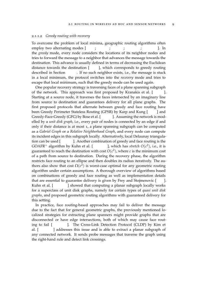
2.1.1.2 Greedy routing with recovery

To overcome the problem of local minima, geographic routing algorithms oftenemploy two alternating modes [KK00

.

; Bos+01

.

; LLM06

.

; KWZ08a

.

; KWZ08b

.

]. Inthe greedy mode, every node considers the locations of its neighbor nodes andtries to forward the message to a neighbor that advances the message towards thedestination. This advance is usually defined in terms of decreasing the Euclideandistance towards the destination [GG12

.

], which corresponds to greedy routingdescribed in Section 2.1.1.1

.

. If no such neighbor exists, i.e., the message is stuckin a local minimum, the protocol switches into the recovery mode and tries toescape that local minimum, such that the greedy mode can be used again.

One popular recovery strategy is traversing faces of a plane spanning subgraphof the network. This approach was first proposed by Kranakis et al. [KSU99

.

].Starting at a source node, it traverses the faces intersected by an imaginary linefrom source to destination and guarantees delivery for all plane graphs. Thefirst proposed protocols that alternate between greedy and face routing havebeen Greedy Perimeter Stateless Routing (GPSR) by Karp and Kung [KK00

.

] andGreedy-Face-Greedy (GFG) by Bose et al. [Bos+01

.

]. Assuming the network is mod-elled by a unit disk graph, i.e., every pair of nodes is connected by an edge if andonly if their distance is at most 1, a plane spanning subgraph can be computedas a Gabriel Graph or a Relative Neighborhood Graph, and every node can computeits incident edges in this subgraph locally. Alternatively, local Delaunay triangula-tion can be used [Gao+05

.

]. Another combination of greedy and face routing is theGOAFR+ algorithm by Kuhn et al. [KWZ08b

.

], which has stretch O(c2), i.e., it isguaranteed to reach the destination with cost O(c2), where c is the minimum costof a path from source to destination. During the recovery phase, the algorithmrestricts face routing to an ellipse and then doubles its radius iteratively. The au-thors also show that cost Ω(c2) is worst-case optimal for any geometric routingalgorithm under certain assumptions. A thorough overview of algorithms basedon combinations of greedy and face routing as well as implementation detailsthat are essential to guarantee delivery is given by Frey and Stojmenovic [FS06

.

].Kuhn et al. [KWZ08a

.

] showed that computing a planar subgraph locally worksfor a superclass of unit disk graphs, namely for certain types of quasi unit diskgraphs, and proposed geometric routing algorithms with guaranteed delivery forthis setting.

In practice, face routing-based approaches may fail to deliver the messagedue to the fact that for general geometric graphs, the previously mentioned lo-calized strategies for extracting plane spanners might provide graphs that aredisconnected or have edge intersections, both of which may cause face rout-ing to fail [Kim+05b

.

]. The Cross-Link Detection Protocol (CLDP) by Kim etal. [Kim+05a

.

] addresses this issue and is able to extract a planar subgraph ofany connected network. It sends probe messages that traverse the graph usingthe right-hand rule and detect link crossings.

10 related work

An additional problem of face routing is that routes tend to hug the hole bound-aries, and due to the resulting uneven load distribution in the network, through-put capacity is reduced [SSG07

.

] and boundary nodes tend to deplete their batter-ies more quickly than other nodes [GG12

.

].Leong et al. [LLM06

.

] use a recovery mode that is alternative to face routing.The proposed Greedy Distributed Spanning Tree Routing (GDSTR) algorithmcomputes and maintains hull trees, which are spanning trees of the network inwhich every tree vertex is annotated by a convex hull of all vertices in its subtree.This information is used when the tree is traversed during the recovery mode.This approach has been extended to the three-dimensional scenario by Zhou etal. [Zho+10

.

].

2.1.1.3 Local routing on geometric graphs

A related line of research considers local geometric routing algorithms on geomet-ric graphs [Bos+02

.

; BM04

.

; DKN10

.

; Bos+15

.

]. In this setting, the nodes are ver-tices of a geometric graph, and every node u decides which neighbor to forwardthe message to based on the following information: the destination, a subsetof other nodes (typically the neighbors of u), a neighbor v of u that has for-warded the message to u (the predecessor) as well as a number of state bits storedin the message, which u can modify before sending. A local geometric rout-ing algorithm is predecessor-oblivious, if the knowledge of the predecessor is notrequired, and predecessor-aware otherwise. This model generalizes greedy rout-ing, compass routing and greedy-compass routing, all of which are predecessor-oblivious and require no state bits, as well as face routing, which is predecessor-aware and requires Θ(log n) state bits for guaranteed delivery on general planargraphs [Bos+15

.

]. For convex subdivisions, face routing only requires predecessor-awareness and the knowledge of the source node to guarantee delivery [KSU99

.

].Durocher et al. [DKN10

.

] showed that a predecessor-aware local geometric routingalgorithm requiring no state bits can not succeed on all geometric unit ball graphs,i.e., graphs in which vertices are points in R3 and are adjacent if and only if thedistance between them is at most 1. For local routing on convex subdivisionswith guaranteed delivery, Bose et al. [Bos+15

.

] presented a predecessor-obliviousalgorithm requiring one state bit and a predecessor-aware algorithm requiring nostate bits. For more results on this topic, we refer to the survey by Durocher etal. [DGW15

.

].

2.1.1.4 Routing with virtual coordinates

An elegant approach proposed to tackle the issues of geographic routing de-scribed in Sections 2.1.1.1

.

and 2.1.1.2

.

is to assign new, synthetic coordinates tothe nodes and then use these virtual coordinates for geometric routing [Rao+03

.

;LLM07

.

; Sar+09

.

; Wat+09

.

; Sar+10

.

]. The virtual coordinates are computed using thetopology of the network. This is particularly advantageous if no real geographiccoordinates are known, for example, if the nodes are not equipped with GPS re-

2.1 routing in wireless ad hoc and sensor networks 11

ceivers. When computing the virtual coordinates, a typical goal is to optimizethe success rate of greedy routing. The first such algorithm was NoGeo by Raoet al. [Rao+03

.

]. First, the algorithm identifies perimeter nodes and assigns tothem fixed locations in the Euclidean plane that lie on a circle. After that, everynon-perimeter node iteratively assigns to itself the center of mass of the currentcoordinates of its neighbors. This is similar to rubber band embeddings [LLW88

.

]and force-directed graph drawing algorithms [Kob12

.

]. Greedy routing on thesevirtual coordinates works well in practice, although successful delivery can not beguaranteed. In a similar spirit, Leong et al. [LLM07

.

] compute virtual coordinatesusing a system of springs and repulsion forces. In particular, a node s is pushedaway from a non-neighbor t, if t is closer to s than any of the neighbors of s. Inthe approach by Watteyne et al. [Wat+09

.

], the nodes initially have random virtualcoordinates which are later updated similarly to the center of mass strategy usedin the NoGeo algorithm [Rao+03

.

].Sarkar et al. [Sar+09

.

] consider dense sensor networks with few holes. Theiralgorithm extracts a plane mesh from the network and augments it using vir-tual nodes and edges, such that the union of triangular faces forms a 2-manifold.Then, the authors apply discrete Ricci flow [CL03

.

] to compute a plane straight-lineembedding of the resulting mesh, such that every non-triangular face is mappedto a circle. The virtual coordinates are computed using a local gossip-style algo-rithm. The authors show that a modification of the standard greedy geometricrouting guarantees delivery on the resulting embedding, i.e., in some cases, mes-sages might be forwarded to virtual nodes associated with the edges of the mesh.In a later work, Sarkar et al. [Sar+10

.

] achieve improved load balancing by utilis-ing geometric properties of their network embedding. Intuitively, they bend theroutes away from the hole boundaries to improve the battery life of boundarynodes, which otherwise tend to deplete fastest. For further methods that use dis-crete Ricci flow to compute virtual coordinates for geometric routing, we refer tothe survey by Gao et al. [GGL15

.

]. Alternatively, Xia et al. [XWJ14

.

] use discreteYamabe flow and compute embeddings in which hole boundaries are mapped totheir convex hulls instead of to circles, which reduces distortion.

Virtual coordinates are not always points in the Euclidean plane. Newsome andSong [NS03

.

] use polar virtual coordinates. Their approach is based on routing ona spanning tree with additional edges between nodes of the same level. Everysubtree of the tree is assigned an angular range that is proportional to the subtreesize. These angular ranges are used as virtual coordinates for routing.

Several approaches are based on selecting a subset of nodes as anchors or land-marks [Car+05

.

; Fan+05

.

; Fon+05

.

; CA06

.

; LA06

.

; Ngu+07

.

; FM07

.

]. Every node in thenetwork computes its hop distances to these landmarks, and the tuples of hopdistances are used as virtual coordinates. Greedy routing combined with vari-ous recovery strategies is then used on these coordinates. For example, Caruso etal. [Car+05

.

], Cao and Abdelzaher [CA06

.

] as well as Liu and Abu-Ghazaleh [LA06

.

]use the Euclidean distance metric for routing, whereas in Beacon Vector Routingby Fonseca et al. [Fon+05

.

], a message is pulled towards landmarks that are closer

12 related work

to the destination than the current node and pushed away by landmarks thatare further away from the destination. Liu and Abu-Ghazaleh [LA06

.

] update thevirtual coordinates by averaging among neighbors to increase the success rate ofgreedy routing, which is similar to the NoGeo algorithm [Rao+03

.

].

2.2 greedy embeddings

The routing algorithms mentioned in Section 2.1.1.4

.

aim at computing virtualcoordinates on which greedy routing has high success rate. A complementary lineof work studies the question, for which network topologies virtual coordinatescan be constructed, such that greedy routing has delivery guarantee of 100%.Stated more formally, we want to find out which graphs have a greedy embedding.Recall that a greedy embedding of a graph is a mapping of its vertices into ametric space, such that greedy routing on the resulting vertex coordinates usingthe corresponding distance metric always succeeds; see Chapter 1

.

.

2.2.1 Graphs admitting Euclidean greedy embeddings

The question about the existence of greedy embeddings for various metric spacesand classes of graphs has attracted a lot of interest from the graph drawing andcomputational geometry communities, the Euclidean plane being the most popu-lar metric space considered. One example of graphs admitting a greedy embed-ding are Delaunay-realizable graphs, since greedy routing is known to alwayssucceed on Delaunay triangulations [BM04

.

]. Another simple example are graphswith a Hamiltonian path, for example, 4-connected planar graphs [TY94

.

]. Pa-padimitriou and Ratajczak [PR05

.

] showed that every graph that is planar and 3-connected (i.e., a removal of at most two vertices never disconnects the graph) hasa greedy embedding in R3 with a custom distance metric that is not the Euclideandistance. They presented a family of graphs that have no greedy embedding in R2

with the Euclidean distance metric, namely Kk,5k+1 (e.g., K1,6 is a star with sixleaves). Furthermore, they showed that a convex graph drawing in R2 in whichall angles are at most 120 is greedy. Finally, they conjectured that all 3-connectedplanar graphs have a greedy embedding in R2 with the Euclidean distance metric.Dhandapani [Dha10

.

] proved that every 3-connected planar triangulation has a pla-nar greedy drawing that is a modification of a classical Schnyder drawing [Sch90

.

].The conjecture by Papadimitriou and Ratajczak itself has been proved indepen-dently by Leighton and Moitra [LM10

.

] and Angelini et al. [AFG10

.

]. Both worksshow this by constructing a greedy drawing for an arbitrary binary cactus graphand use the fact that such spanning graph exists for every 3-connected planargraph. Leighton and Moitra [LM10

.

] also gave an example of a binary tree forwhich no greedy embedding exists. Nöllenburg and Prutkin [NP17

.

] character-ized trees admitting a greedy embedding; see Chapter 4

.

of this thesis. Recently,Da Lozzo et al. [DDF17

.

] showed that every 3-connected planar graph admits a pla-

2.2 greedy embeddings 13

nar greedy embedding. The strong Papadimitriou-Ratajczak conjecture that every3-connected planar graph admits a convex greedy embedding still remains open.

2.2.2 Non-Euclidean greedy embeddings

Kleinberg [Kle07

.

] showed that every connected graph has a greedy embeddingin the hyperbolic plane. He also described a distributed algorithm, using whichevery node can compute its coordinates in such an embedding. The algorithm isbased on distributed computation of a rooted spanning tree. Flury et al. [FPW09

.

]construct greedy embeddings of combinatorial unit disk graphs (unit disk graphswithout geometric information) in spaces of O(log2 n) dimensions with boundedhop stretch, i.e., edge counts in paths resulting from greedy routing with the pro-posed virtual coordinates exceed the lengths of the corresponding shortest pathsby at most a constant factor. Ben Chen et al. [Ben+11

.

] present a greedy embed-ding scheme for 3-connected planar graphs with a non-Euclidean routing metricbased on power diagrams. The virtual coordinates are computed in a distributedfashion using the Thurston algorithm for computing a circle packing [Thu85

.

].

2.2.3 Succinctness

Since efficient use of storage and bandwidth are crucial in wireless sensor net-works, virtual coordinates should require only few, i.e., O(log n), bits in orderto keep message headers small. Greedy drawings with this property are calledsuccinct. The constructions by Kleinberg [Kle07

.

], Leighton and Moitra [LM10

.

]and Angelini et al. [AFG10

.

] do not guarantee succinctness, and the resulting vir-tual coordinates may require high precision in order to be represented explicitly.For example, when using the hyperbolic embedding by Kleinberg [Kle07

.

], Xia etal. [XWJ14

.

] observed routing errors in their simulations caused by insufficient pre-cision (using 64-bit doubles and networks with less than 300 000 nodes). Angeliniet al. [ADF12

.

] showed that greedy drawings of trees sometimes require exponen-tial area. Eppstein and Goodrich proved the existence of greedy drawings for anyconnected graph in the hyperbolic plane [EG11

.

], in which virtual coordinates canbe encoded succinctly, and Goodrich and Strash [GS09

.

] showed it for 3-connectedplanar graphs in R2. Wang and He [WH14

.

] used a custom distance metric andconstructed convex, planar and succinct drawings for 3-connected planar graphsusing Schnyder realizers [Sch90

.

]. In the approach by Flury et al. [FPW09

.

], vir-tual coordinates require O(log3 n) bits. Zhang and Govindaiah [ZG13

.

] constructgreedy embeddings into a semi-metric space that consists of tuples of integers be-tween 1 and 2n− 2. Such virtual coordinates are computed by a simple traversalof a spanning tree, and every tuple consists of at most ∆ integers, ∆ being themaximum degree of the tree. In this way, it is possible to construct O(log n) bitvirtual coordinates for 3-connected planar graphs or any graphs with a spanningtree that has constant maximum degree.

14 related work

Succinct greedy embeddings can be considered a special case of compact routingschemes [TZ01

.

]. In that setting, every node is labeled using a small, typicallypolylogarithmic, number of bits. The label of the destination is stored in themessage header, possibly along with some additional information, and routingdecisions are made locally at every node based on the message header and aprecomputed routing table of the node. For example, by storing routing tables ofsize O(n1/k) at every node and using O(k log2 n) bit labels, routing with stretch4k− 5 can be achieved [TZ01

.

] (O hides a polylogarithmic factor). For an overviewof related results, we refer the reader to the survey by Chechik [Che14

.

].A labelling scheme for ancestor queries of a rooted tree is an assignment of labels to

the tree nodes, such that the labels of two nodes u and v are sufficient to determinewhether u is an ancestor of v in constant time [KNR92

.

]. Such a labeling can beused for local routing on the tree. Dahlgaard et al. [DKR15

.

] presented a labellingscheme for ancestor queries with labels of size log2 n + 2 log2 log2 n + 3. Suchlabels can be viewed as succinct virtual coordinates for local routing.

2.3 graph drawings with geodesic-path tendency

Finding paths in a graph embedding that always make progress towards theirdestination, as is the case for greedy routing considered in Section 2.1.1.1

.

, is mo-tivated not only by geographic routing in wireless ad hoc and sensor networks.Studies have shown that such paths are easier to trace for users when exploring agraph drawing. Using eye tracking, Huang et al. [HE05

.

; Hua07

.

] discovered thatpeople exhibit geodesic-path tendency, i.e., when eyes encounter nodes with morethan one link, the link that goes towards the node is more likely to be searchedfirst. This tendency has been validated by user experiments, in which the taskwas to find shortest paths in a graph drawing [HEH09

.

]. For example, it has beenshown that dead-ends that go towards the target node slow down graph reading.Another notion that has been shown to be important for the readability of graphdrawings is path continuity, i.e., smooth, continued paths are traced easier thanzigzags or paths that detour [War+02

.

; Pur+12

.

]. Not surprisingly, graph drawingsin which a path with certain geometric properties exists between every pair ofvertices have become a popular research topic. Over the last years a number ofdifferent drawing conventions implementing the notion of strong geodesic-pathtendency and path continuity have been suggested, namely the aforementionedgreedy drawings [Rao+03

.

] as well as (strongly) monotone drawings [Ang+12

.

], self-approaching and increasing-chord drawings [Ala+13

.

].

2.3.1 Monotone drawings

While getting closer to the destination in each step, a distance-decreasing path in agreedy drawing can make numerous turns and may even look like a spiral, whichhardly matches the intuitive notions of geodesic-path tendency and path continu-

2.3 graph drawings with geodesic-path tendency 15

ity. To overcome this, Angelini et al. [Ang+12

.

] introduced monotone drawings,where one requires that for every pair of vertices s and t there exists a monotonepath, i.e., a path that is monotone with respect to some direction. Ideally, thatmonotonicity direction should be

#»st. This property is called strong monotonicity.Angelini et al. [Ang+12

.

] showed that every tree has a monotone drawing ona grid of area O(n1.6) × O(n1.6) or O(n) × O(n2). He and He [HH17

.

] showedthat the grid area can be reduced to 12n× 12n, which is asymptotically optimal.Oikonomou and Symvonis [OS17

.

] improved the grid area further to n× n. Arkinet al. [ACM89

.

] studied the problem of finding monotone paths between a pair ofpoints among a set of disjoint obstacles and showed that such path always existsif all obstacles are convex. This implies that all strictly convex graph drawings(i.e., every face is a convex polygon without flat angles) are monotone [Ang+12

.

;HH15

.

]. Angelini et al. [Ang+12

.

] showed that biconnected planar graphs admitplanar monotone drawings, and Hossain and Rahman [HR15

.

] showed that thisis the case for all planar graphs. He and He [HH15

.

] showed that the classicalSchnyder drawings of 3-connected planar graphs are monotone, even though theyare not always strictly convex.

The question of finding plane monotone drawings that preserve the planar em-bedding of the input graph has also been studied. In this setting, Angelini etal. [Ang+15

.

] proved that all plane graphs admit plane monotone drawings withfew bends and that in the special case of biconnected embedded planar graphsand outerplane graphs, there exist plane monotone drawings with straight lines.

In a monotone drawing, the directions with respect to which a monotone pathexists might be different for different pairs of vertices. To make the task of find-ing paths easier for a user, the direction of monotonicity should be easy to deter-mine. Therefore, it is desirable to limit the number of such possible monotonic-ity directions. He and He [HH15

.

] considered the classical Schnyder drawingsof 3-connected planar graphs and showed that there exist six fixed intervals ofdirections, such that between every pair of vertices there exists a path that ismonotone with respect to all directions of one of the intervals. Angelini [Ang17

.

]also considered the classical Schnyder drawings and showed that for 3-connectedplanar graphs, three monotonicity directions are sufficient, and two are sufficientin Schnyder drawings of maximal planar graphs. In the same work, graphs forwhich a single monotonicity direction suffices have been characterized.

In strongly monotone drawings, for every pair of vertices s, t there exists a paththat is monotone with respect to the direction

#»st. Kindermann et al. [Kin+14

.

]showed that every tree admits a strongly monotone drawing and, therefore, sodoes every connected graph, if crossings are allowed. Felsner et al. [Fel+16

.

]showed that planar strongly monotone drawings exist for 3-connected planargraphs, outerplanar graphs and 2-trees.

16 related work

s

t

Figure 10: The thick blue zigzag path is the shortest distance-decreasing st-path in thegreedy drawing. Figure from a joint work with Angelini et al. [Ang+18

.

].

2.3.2 Geometric spanners

Distance-decreasing paths in a greedy drawing as well as monotone paths mayhave arbitrarily large detour, i.e., the ratio between the geometric length of a pathand the distance of its endpoints can, in general, not be bounded by a constant.Bounding the detour is a popular objective in the area of geometric network de-sign. Given a set of points in the plane, the task is to connect the points with fewedges, such that every pair of points in the network is connected by a path withbounded detour. Geometric networks with this property are called spanners, andthe maximum detour of a shortest path between a pair of vertices in a geometricnetwork is called dilation. Chew [Che89

.

] used a variant of Delaunay triangulationand was the first to show that planar spanners with bounded dilation exist forevery point set. The standard Euclidean Delaunay triangulation is also a planarspanner [DFS90

.

]. For an overview of the various techniques to construct planargeometric spanners, we refer to the comprehensive surveys by Eppstein [Epp00

.

],Narasimhan and Smid [NS07

.

] and Bose and Smid [BS13

.

]. Spanners in whichpaths with bounded detour can be found by local routing (see Section 2.1.1.3

.

)have also been studied [Bos+12

.

; Bon+17

.

]. Schindelhauer et al. [SVZ07

.

] consideredweak spanners and power spanners, which are relaxations of geometric spanners.For some constant c and for every pair of vertices s, t, in a weak c-spanner thereexists an st-path that remains within a circle around s with radius c|st|. For con-stants c and δ, in a (c, δ)-power spanner, there exists an st-path for every pair ofvertices s, t, such that the sum of the δth powers of the path’s edge lengths is atmost c|st|δ. The authors showed that weak spanners are power spanners, but notnecessarily vice versa. It is easy to see that greedy drawings are weak 2-spannersand, consequently, power spanners. To the best of my knowledge, it is still openwhether greedy drawings are geometric spanners. In Chapter 5

.

, I show that thisis the case for greedy drawings of trees and cactuses.

2.3.3 Self-approaching and increasing-chord drawings

Motivated by the notion of bounded detour, Alamdari et al. [Ala+13

.

] initiated thestudy of self-approaching graph drawings. Self-approaching curves, introduced byIcking et al. [IKL99

.

], are curves where for any point t′ on the curve, the distanceto t′ is continuously non-increasing while traversing the curve from the start to t′.Equivalently, a curve is self-approaching if, for any three points a, b, c in thisorder along the curve, we have |ac| ≥ |bc|. An even stricter requirement are

2.3 graph drawings with geodesic-path tendency 17

a

b c

d

f

gh

e

i

j

Figure 11: A self-approaching graph drawing that is not monotone. Neither one of thetwo a- f -paths is monotone in any direction. Dashed lines are edge normals.

so-called increasing-chord curves, which are curves that are self-approaching inboth directions. The name is motivated by the characterization of such curves,which states that a curve has increasing chords if and only if for any four distinctpoints a, b, c, d in that order, we have |bc| ≤ |ad|. Self-approaching curves havedetour at most 5.333 [IKL99

.

], and increasing-chord curves have detour at most2.094 [Rot94

.

]. Note that in greedy drawings, bounding the detour of the shortestdistance-decreasing path between a pair of vertices by a constant is impossible ingeneral; see Figure 10

.

.Alamdari et al. [Ala+13

.

] gave a complete characterization of trees admittingself-approaching drawings. Nöllenburg et al. [NPR16

.

] showed that every triangu-lation admits a (not necessarily planar) increasing-chord drawing and that everyplanar 3-tree admits a planar increasing-chord drawing; see Chapter 5

.

. Notethat deciding whether two vertices are connected by a self-approaching path in astraight-line graph drawing is NP-hard for three-dimensional drawings [Ala+13

.

]and is conjectured to be NP-hard in two dimensions as well [Bah+17

.

]. Thus,unlike for greedy drawings, recognizing whether a given graph drawing is self-approaching might be NP-hard. Furthermore, Alamdari et al. [Ala+13

.

], Frati etal. [DFG15

.

] and Mastakas and Symvonis [MS15

.

] investigated the problem of con-necting given points to obtain an increasing-chord drawing. A special case ofincreasing-chord graph drawings are angle-monotone graph drawings, in whichevery pair of vertices is joined by a path that is, after some rotation, both x- andy-monotone [Bon+16

.

; LO17

.

].Every increasing-chord drawing is self-approaching as well as strongly mono-

tone [Ala+13

.

], but a strongly monotone drawing is not necessarily self-approach-ing. A self-approaching drawing is greedy, but not necessarily monotone (seeFigure 11

.

), and a greedy drawing is generally neither self-approaching nor mono-tone. Greedy drawings of trees are monotone (Angelini et al. [ADF12

.

] showedthat such drawings are slope-disjoint, which implies monotonicity [Ang+12

.

]). Fur-thermore, for trees, the notions of self-approaching and increasing-chord drawingcoincide since all paths are unique. An overview of existence results for a selec-tion of popular and important classes of planar graphs is given in Table 1

.

. Tothe best of my knowledge, no graphs are known that admit a self-approachingdrawing, but no increasing-chord drawing.

18 related work

Table1:A

noverview

ofexistence

resultsof

greedy,monotone,strongly

monotone

andincreasing-chord

drawings

forpopular

classesof

planargraphs.The

highlightedresults

arepresented

inC

hapters4

.

and5

.

ofthis

thesis.

greedym

onotonestrongly

monotone

increasing-chord

treescharacterized

[NP17

.

]alw

ays[A

ng+12

.

]alw

ays[K

in+14

.

]characterized

[Ala+13

.

]

binarycactuses

always,planar

[ LM10

.

;AFG

10

.

]alw

ays,even

allouterplane,preserve

embedding

[ Ang+15

.

]

always,even

allouterplane,convex

andpreserve

embedding

[ Fel+16

.

]

notalw

ays[N

PR16

.

]

triangulationsalw

ays,planar[D

ha10

.

]alw

ays,planar[A

CM

89

.

;HH

15

.

;Ang17

.

]alw

ays,planar[Fel+16

.

]alw

ays[N

PR16

.

];planarity

inspecialcases,

openin

general

3-connectedplanar

graphsalw

ays[LM

10

.

;AFG

10

.

],planar

[DD

F17

.

],convexity

open

always,planar

[HH

15

.

;Ang17

.

]alw

ays,planar[Fel+16

.

]open

connectedplanar

notalw

ays[PR

05

.

]alw

ays,planar[ H

R15

.

]planarity:not

always,

openfor

biconnected[ Fel+16

.

]

notalw

ays[PR

05

.

]

2.4 greedy geometric routing in continuous domains 19

2.4 greedy geometric routing in continuous domains

Let us now return to wireless sensor networks and consider a network of sen-sors distributed over a closed region. An assumption often made in the litera-ture is that the distribution of the sensors is very dense, except for relatively fewholes [Sar+09

.

; TK12

.

; Bir13

.

]. Assuming the density of nodes within the networkboundary is close to infinity, greedy routing will forward a message along thestraight line towards its destination or, if the boundary is hit, the message willslide along the boundary, as long as it decreases the Euclidean distance to thedestination.

2.4.1 Beacon-based routing

For the above setting, Biro et al. [Bir+11

.

] proposed the beacon-based routing model.A message is modeled by a point that moves inside a polygonal region P , insidewhich there exists a set of beacons. When activated, a beacon creates a magneticpull everywhere inside P , such that a point in P either moves towards the beaconalong the straight line, or, if the boundary is hit, slides along the boundary, aslong as the distance to the beacon decreases continuously. Once decreasing thedistance to the beacon is no longer possible, the point gets stuck. Only one beaconis active at each point in time, and when it is reached by the moving point, thebeacon is deactivated, and another one can be activated. Points s, t are routedif there exists a sequence of beacons ending with t, such that the beacons areactivated consecutively and such that every currently active beacon is reachedby s eventually and then deactivated. The authors studied the complexity ofcovering, or guarding, polygonal regions with few beacons, such that all pairs ofpoints are routed. Here, the beacons for the destinations are not counted, sinceotherwise every point in the region must be a beacon. In a follow-up work, Biroet al. [Bir+13

.

] designed algorithms to select a minimum sequence of beacons toforward a message to a given destination point. Various routing and guardingproblems in the beacon-based routing model were covered in detail by MichaelBiro in his dissertation [Bir13

.

].Beacon-based routing is related to landmark-based techniques for routing in

wireless sensor networks mentioned in Section 2.1.1.4

.

. Recall that in these tech-niques, routing decisions at every node are made based on distances to a subsetof designated landmark nodes. For example, in Gradient Landmark-Based Dis-tributed Routing (GLIDER) by Fang et al. [Fan+05

.

], the network is partitionedinto Voronoi cells of the landmark nodes, i.e., all nodes inside a cell have a clos-est landmark in common with respect to hop distance. The adjacency graph ofthe cells is used to route messages to a different cell, whereas greedy routing onvirtual coordinates is used for intra-cell routing.

20 related work

2.4.2 Network decomposition for routing

Similar to GLIDER [Fan+05

.

], other approaches decompose the network into com-ponents such that in each of them greedy routing or variants thereof are likelyto perform well [BGJ07

.

; FM07

.

; TBK09

.

; ZSG09

.

; TK12

.

; Jia+15

.

]. A global datastructure of preferably small size is used to store interconnectivity between com-ponents. One such network decomposition approach proposed by Tan and Ker-marrec [TK12

.

] will be considered in detail here. The authors assume that globalconnectivity irregularities, i.e, large holes in the network and the network bound-ary, are the main source of local minima in which greedy routing between a pairof sensor nodes might get stuck. They note that in practical sensor networks,local connectivity irregularities normally have low impact on the cost of routingand the quality of the resulting paths, since the local minima in this context canbe overcome by simple and light-weight techniques; see [TK12

.

] for a list of suchstrategies. With this reasoning, Tan and Kermarrec model the network as a polyg-onal region with obstacles or holes inside it and consider greedy routing insidethis continuous domain, similarly to the beacon-based routing model proposedby Biro et al. [Bir+11

.

]. Local minima now only appear on the boundaries of thepolygonal region. In Chapter 6

.

, the same model is used.Tan and Kermarrec [TK12

.

] try to partition this region into a minimum numberof polygons, in which greedy routing works between every pair of points. Theycall such components greedily routable regions (GRRs). For intercomponent routing,region adjacencies are stored in a graph. In the continuous setting, the algorithmis able to guarantee finding paths with bounded detour.

For routing in the underlying network of sensor nodes corresponding to dis-crete points inside the polygonal region, greedy routing is used if the source andthe destination nodes are in the same component, and existing techniques areused to overcome local minima. For inter-component routing, every node storesa neighbor on a shortest path to each component. This information is used to getto the component of the destination, and then intra-component routing is used.

Tan and Kermarrec [TK12

.

] emphasize the importance for the nodes to store assmall routing tables as possible and note that the size of a node’s routing tabledirectly reflects the number of network components in a decomposition. There-fore, the goal is to partition the network into a minimum number of GRRs. Theauthors prove that partitioning a polygonal region with holes into a minimumnumber of GRRs is NP-hard and propose a simple heuristic. Its solution maystrongly deviate from the optimum even for very simple polygons; see the exam-ples in Chapter 6

.

.The problem of partitioning a polygonal region into a minimum number of

GRRs is strongly reminiscent of partitioning a polygonal region into a minimumnumber of convex subpolygons, which is a well-studied problem from computa-tional geometry. For an overview of the results on the convex partition problem,see the survey by Keil [Kei00

.

]. For polygonal regions with holes, minimum con-vex partition is known to be NP-hard if Steiner points are allowed (i.e., cuts of the

2.4 greedy geometric routing in continuous domains 21

(a) (b)

Figure 12: A benchmark instance of the GRR decomposition problem. Figure taken fromthe work of Tan and Kermarrec [TK12

.

]. (a)

.

A network of streets over whichwireless sensor nodes are densely distributed. (b)

.

The resulting network isapproximated as a thin polygonal region and partitioned into GRRs.

partition are not necessarily diagonals of the input polygonal region) [Lin82

.

], aswell as if no Steiner points are allowed [Kei85

.

]. Therefore, it is not completelyunexpected that the minimum GRR partition problem for polygonal regions withholes is NP-hard as well. For simple polygons without holes, however, minimumconvex partitions both with and without Steiner points can be computed in poly-nomial time [Kei85

.

; CD85

.

], and approximate solutions can be computed usingsimple strategies. For example, the naive strategy of iteratively cutting along thebisectors of reflex angles provides an approximation of factor 2 for the minimumpartition with Steiner points of simple hole-free polygons [CD85

.

]. It is thereforesurprising that for minimum GRR partition of simple polygons without holes, nopolynomial-time optimal solutions or even constant-factor approximations wereproposed.

Some benchmark instances from the work of Tan and Kermarrec [TK12

.

, Fig-ure 17] are networks of sensor nodes distributed on roads of a city; see Figure 12

.

.The resulting polygonal regions are very narrow and strongly resemble planestraight-line graph drawings. Therefore, considering plane straight-line graphdrawings in addition to polygonal regions is a natural adjustment of the mini-mum GRR partition problem. In this scenario, GRRs coincide with increasing-chord drawings of trees as studied by Alamdari et al. [Ala+13

.

]. I approach thisproblem in Chapter 6

.

of this thesis.Recently, Bose et al. [BKL17

.

] studied the complexity of finding shortest self-approaching paths in simple polygons. Additionally, the authors characterizedself-approaching polygons, i.e., polygons in which every pair of points can beconnected by a self-approaching path, and provided a linear-time algorithm to rec-ognize such polygons. From this characterization, it follows that self-approaching

22 related work

polygons are exactly the greedily routable regions studied by Tan and Kermar-rec [TK12

.

] and in Chapter 6

.

of this thesis.

3P R E L I M I N A R I E S

This chapter recalls several graph-theoretic concepts and defines notation that willbe used in this thesis.

3.1 graphs , paths and connectivity

A graph is a mathematical object that is often used to model relationships between graph

entities. Formally, a graph is a tuple G = (V, E), where V = v1, . . . , vn is a setof vertices and E = e1, . . . , em a set of edges, such that every edge e ∈ E is atuple e = u, v for vertices u, v ∈ V. For brevity, we write uv instead of u, v.We call a pair of vertices u, v ∈ V adjacent, if uv ∈ E. For an edge e = uv ∈ E, wesay that u and v are endpoints of e and that both u and v are incident to e. Edges e1,e2 are incident to each other, if they share a common endpoint. The degree deg(v)of a node v is the number of edges incident to v in G. We call vertices adjacent toa vertex v ∈ V the neighbors of v. Let N(v) denote the neighbors of v in G.

A path in G is a tuple ρ = (v0, v1, . . . , vk), such that vivi+1 ∈ E for i = 0, . . . , k− 1.We say that ρ has length k. For vertices s, t ∈ V, such that s = v0 and t = vk, wecall such a tuple (v0, v1, . . . , vk) an s-t-path (or st-path) in G. A path is simple, if vi s-t-path

are pairwise distinct, for i = 0, . . . , k.We say that s, t ∈ V have distance k in G, if the minimum length of an st-path distance dG(s, t)

in Gin G is k. We write dG(s, t) = k. For k ∈ N, k ≥ 1, the k-neighborhood Nk(v) of anode v ∈ V is defined as Nk(v) = u ∈ V | dG(v, u) ≤ k.

For a path ρ = (v0, v1, . . . , vk) and 0 ≤ p ≤ q ≤ k, we call (vp, . . . , vq) a subpathof ρ. A path (v0, v1, . . . , vk), k ≥ 3, is a cycle, if v0 = vk. A cycle (v0, v1, . . . , vk) issimple, if for i = 1, . . . , k− 1, all vertices vi are pairwise distinct.

A graph G1 = (V1, E1) is a subgraph of a graph G = (V, E), if we have V1 ⊆ Vand E1 ⊆ E. Such a subgraph G1 is a spanning subgraph of G, if V1 = V.

For a pair of vertices s, t ∈ V, we say that s and t are connected in G if an st-pathexists in G. A graph G is connected, if every pair of its vertices is connected in G.A connected component is an inclusion-maximal connected subgraph of G.

If no cycle exists in G, then G is a forest. A tree is a connected forest. A subtree isa subgraph of a tree that is a tree itself. A leaf of a tree is a tree vertex of degree 1.

For a graph G = (V, E) and vertex set V ′ ⊆ V, let G−V ′ denote the graph with G−V′, G± E′

vertex set V \ V ′ and edge set uv ∈ E | u, v ∈ V \ V ′. For an edge set E1 ⊆ E,

23

24 preliminaries

Figure 13: A binary or Christmas cactus graph.

let G − E1 denote the graph with vertex set V and edge set E \ E1. For an edgeset E2, let G + E2 denote the graph with vertex set

V ∪ u | u is an endpoint of an edge in E2

and edge set E ∪ E2. We write G − v instead of G − v and G ± uv insteadof G± uv.

Let G = (V, E) be a connected graph. A separating k-set is a set S ⊆ V ofk vertices whose removal disconnects the graph, i.e., G − S is disconnected. Avertex forming a separating 1-set is called cutvertex. A graph is c-connected if itc-connected

does not admit a separating k-set with k ≤ c − 1; 2-connected graphs are alsocalled biconnected. A connected graph is biconnected if and only if it does notcontain a cutvertex. A block is a maximal biconnected subgraph.block

A subdivision of a graph G = (V, E) is a graph created by replacing every edgein a set E1 ⊆ E by a simple path.

A caterpillar is a tree T, such that the graph created by removing all leaves of Tis a path. A tree is a star if it has exactly one vertex v with deg(v) ≥ 2. A starwith d leaves is denoted by K1,d.

A rooted tree T is a tree T = (V, E) together with a distinguished vertex r ∈ Vcalled root. A subtree of a node v is then the subtree of T with root v containing allvertices u, for which the u-r-path in T contains v. A parent of v ∈ V is a neighbor uof v that is not in the subtree of v.

A cactus is a graph in which every edge is part of at most one simple cycle. Abinary (or Christmas) cactus is a cactus in which every vertex is part of at most twobinary cactus

blocks; see Figure 13

.

.

3.2 graph drawings and polygons

A drawing Γ of a graph G = (V, E) maps every vertex v ∈ V to a point Γ(v) ∈ R2

and every edge uv ∈ E to a simple open curve Γ(uv) ⊆ R2 with endpoints Γ(u)and Γ(v).

A graph drawing is planar if the curves intersect only at their common end-points, i.e., 1) curves Γ(uv), Γ(xy) have an intersection only if edges uv, xy ∈ Eare incident in G and 2) for edges uv and uw, the only intersection of Γ(uv)

3.2 graph drawings and polygons 25

and Γ(uw) is Γ(u). A graph is planar if it admits a planar drawing. A graph ismaximal planar or a triangulation if no edge can be added to it without violating triangulation

the graph’s planarity.A drawing is straight-line if every Γ(uv) is a straight-line segment. In this thesis,

we only consider graph drawings that are straight-line. If the drawing Γ is fixed,we associate every vertex v ∈ V with the corresponding point Γ(v) and everyedge uv with the corresponding straight-line segment Γ(uv). Straight-line graphdrawings are also called geometric graphs.

A simple polygon (or just polygon) is a closed flat region bounded by a closed simple polygon

chain of straight-line segments that has no self-intersections. A polygonal region is polygonal regiondefined by a simple polygon and m ≥ 0 holes contained inside it, each of whichis a simple polygon.

3.2.1 Greedy, monotone, self-approaching and increasing-chord drawings

For points p, q ∈ R2, let |pq| denote the Euclidean distance between p and q. distance |pq|

Definition 3.1 (Distance-decreasing path). Consider a straight-line graph drawing Γand vertices s, t in Γ. An st-path (s = v0, v1, . . . , vk = t) is distance-decreasing, if we distance-decreasing

pathhave |vi+1t| < |vit| for every i = 0, . . . , k− 1.

Definition 3.2 (Greedy embedding). A straight-line graph drawing Γ of a graph G =

(V, E) is a greedy embedding or a greedy drawing, if for every pair of vertices s, greedy embedding

t ∈ V, s 6= t, there exists a distance-decreasing st-path in Γ.

Equivalently, a straight-line drawing Γ of a graph G = (V, E) is a greedy draw-ing if for every pair of vertices s, t ∈ V, s 6= t, there exists a neighbor u of swith |ut| < |st|.

Definition 3.3 (Self-approaching curve [IKL99

.

]). An oriented curve is self-approach-ing if, for any three points a, b, c in this order along the curve, we have |ac| ≥ |bc|.

Definition 3.4 (Increasing-chord curve [Rot94

.

]). An oriented curve is increasing-chord (or has increasing chords) if, for any four points a, b, c, d in this order along thecurve, we have |bc| ≤ |ad|.

An st-path in a straight-line graph drawing Γ is self-approaching (increasing- self-approaching andincreasing-chordpaths

chord), if the corresponding curve is self-approaching (increasing-chord).

Definition 3.5 (Self-approaching and increasing-chord graph drawings [Ala+13

.

]).A straight-line drawing Γ of a graph G = (V, E) is self-approaching (increasing-chord),if every vertex pair s, t ∈ V is joined by a self-approaching (increasing-chord) st-path.

Definition 3.6 (Monotone and strongly monotone graph drawings [Ang+12

.

]). Astraight-line drawing Γ of a graph G = (V, E) is

1) monotone, if every vertex pair s, t ∈ V is joined by an st-path that is monotone insome direction;

26 preliminaries

2) strongly monotone, if every vertex pair s, t ∈ V is joined by an st-path that ismonotone in direction #»st.

Definition 3.7 (Detour and dilation). 1. For an oriented curve C and points p, q on C,the detour of C between p and q is defined as dC(p,q)

|pq| , where dC(p, q) denotes thedistance from p to q along the curve C.

2. For vertices s, t of a geometric graph Γ, the detour of Γ between s and t is theminimum detour between s and t of a curve corresponding to an st-path in Γ.

3. The vertex dilation of a geometric graph Γ is the largest detour from s to t on Γ overall pairs of vertices s, t of Γ.

In this thesis, dilation of a geometric graph Γ stands for vertex dilation. Otherterms used for dilation in the literature are spanning ratio or stretch factor. Ageometric graph whose dilation is bounded by a constant c is a geometric c-spanner.

3.2.2 Used geometric notation

Let #»e1 and #»e2 be the first and the second standard basis vectors. We say thatvector

#»

d points upwards if the dot product#»

d · #»e2 of#»

d and #»e2 is positive. We say#»

d points upwards,downwards, to the

left, to the rightthat

#»

d points downwards if we have#»

d · #»e2 < 0. We say that#»

d points to the right ifwe have

#»

d · #»e1 > 0. We say that#»

d points to the left if we have#»

d · #»e1 < 0.For the ease of notation, we shall sometimes treat a graph edge uv as an ordered

tuple. For example, for a given straight-line graph drawing Γ, we say that anedge uv points upwards if the vector # »uv points upwards, etc.

For points a, b, c ∈ R2, let ∠abc denote the angle at b formed by ab and bc, suchthat ∠abc ≤ 180. For vectors

#»

ab,#»

cd, let ∠ccw(#»

ab,#»

cd) denote the counterclockwise∠, ∠cw, ∠ccw

turn (or turning angle) from#»

ab to#»

cd. Analogously, let ∠cw(#»

ab,#»

cd) denote theclockwise turn from

#»

ab to#»

cd. We say that point p is inside the angle ∠abc < 180,if either ∠cw(

#»

ba,# »

bp) ≤ ∠cw(#»

ba,#»

bc) < 180 or ∠ccw(#»

ba,# »

bp) ≤ ∠ccw(#»

ba,#»

bc) < 180.Otherwise, we say that p is outside of ∠abc.

For points a, b ∈ R2, let ray(a, b) denote the ray with origin a and direction#»

ab.ray

For a vector#»

d , let ray(a,#»

d ) denote the ray with origin a and direction#»

d .

Part I

G R A P H E M B E D D I N G S M O T I VAT E D B Y G R E E D YR O U T I N G : E X I S T E N C E

4E U C L I D E A N G R E E D Y D R AW I N G S O F T R E E S

In this chapter, we1 completely characterize the trees that admit a greedy embed-ding in R2. This answers a question by Angelini et al. [ADF12

.

] and is a furtherstep in characterizing the graphs that admit Euclidean greedy embeddings. Chap-ter 4

.

is based on joint work with Martin Nöllenburg [NP13

.

; NP17

.

].

4.1 introduction

The question about the existence of greedy embeddings for various metric spacesand classes of graphs has attracted a lot of interest. An overview of related workis presented in Chapter 2

.

of this thesis. We recall that most works on Euclideangreedy embeddings consider 3-connected planar graphs [PR05

.

; AFG10

.

; LM10

.

;Dha10

.

; GS09

.

; DDF17

.

].

4.1.1 Contribution

We give the first complete characterization of all trees that admit a greedy em-bedding in R2 with the Euclidean distance metric. This solves the correspondingopen problem stated by Angelini et al. [ADF12

.

] and is a further step in character-izing the graphs that have greedy embeddings. For any given tree T and an edge eof T separating T into T1 and T2, we calculate a tight upper bound on the openingangle of a cone formed by perpendicular bisectors of edges of T1, in which T2

is contained in any greedy embedding in time linear in the size of T1. We thenshow that deciding whether T has a greedy embedding is equivalent to decidingwhether there exists a valid angle assignment in a certain wheel polygon. This in-cludes a non-linear constraint known as the wheel condition [DV96

.

]. For most cases(all trees with maximum degree 4 and most trees with maximum degree 5) weare able to give an explicit solution to this problem, which provides a linear-timerecognition algorithm. For trees with maximum degree 3 we give an alternativecharacterization by forbidden subtrees. For some trees with one degree-5 node weresort to using non-linear solvers. For trees with nodes of degree ≥ 6 no greedydrawings exist.

1 In the remainder of my thesis, I write “we” instead of “I” for convenience.

29

30 euclidean greedy drawings of trees

Our proofs are constructive, however, we ignore the possibly exponential arearequirements for our constructions. This is justified, since some trees requireexponential-size greedy drawings as shown by Angelini et al. [ADF12

.

].

4.2 preliminaries

In this section, we introduce the concept of the opening angle of a rooted subtreeand present relations between opening angles that will be crucial for the charac-terization of greedy-drawable trees. We start with a number of lemmas on basicproperties of opening angles and greedy drawings and sketch the main ideasof our characterization. This is followed by proving the shrinking lemma, whichserves as a main tool for our later constructions.

It is known that for a greedy drawing Γ of T any subtree of T is representedin Γ by a greedy subdrawing [ADF12

.

]. We define the axis of an edge uv as itsaxis(uv)

perpendicular bisector. The following property of greedy drawings is easy toshow.

Observation 4.1. In a greedy drawing of tree T = (V, E), for every edge uv ∈ E,axis(uv) contains no vertices of T.

Proof. Let vertex w lie on axis(uv). Either the u-w-path or the v-w-path containsedge uv. In both cases, the distance to w must decrease for the nodes of the path,a contradiction to |uw| = |vw|.

Let huuv denote the open half-plane bounded by the axis of uv and containing u.half-plane hu

uv

Let Tuuv be the subtree of T containing u obtained from T by removing uv. The fol-tree Tu

uv

lowing property is the immediate consequence of Observation 4.1

.

and Lemma 3in [ADF12

.

].

Lemma 4.1. In a greedy drawing of tree T = (V, E), for every edge uv ∈ E,

(a) axis(uv) has empty intersection with every edge from E \ uv, and

(b) every subtree Tuuv is contained in hu

uv.

The converse is also true.

Lemma 4.2. Let Γ be a drawing of T with Tuuv ⊆ hu

uv for all uv ∈ E. Then, Γ is greedy.

Proof. For s, t ∈ V let u be the neighbor of s on the unique s-t-path in T. Sincet ∈ Tu

su ⊆ husu, we have |ut| < |st|.

Angelini et al. [ADF12

.

] further showed that greedy tree drawings are alwaysangles > 60

planar and that in any greedy drawing of T the angle between two adjacent edgesmust be strictly greater than 60. Thus T cannot have a node of degree ≥ 6.maximum degree 5

Lemma 4.3 (Lemma 7 in [ADF12

.

]). Consider two edges uv and wz in a greedy drawingof T, such that the path from u to w does not contain v and z. Then, the rays ray(u, # »uv)and ray(w, # »wz) diverge; see Figure 14

.

.

4.2 preliminaries 31

w

u

z

v

Figure 14: Sketch of Lemma 4.3

.

.

Lemma 4.4. Let Γ be a greedy drawing of T = (V, E), v ∈ V, deg(v) = 2, N(v) =

u, w the only two neighbors of v, and T′ = (T− v) + uw. The drawing Γ′ induced by shortcuts

replacing segments uv and vw by uw in Γ is a greedy drawing of T′.

Proof. For x, y in T′, let ρ′ and ρ be the x-y-paths in T′ and in T, respectively.If ρ 6= ρ′, then v ∈ ρ. Since distance to y decreases along ρ, it also decreasesalong ρ′. Hence, Γ′ is greedy.

Let Γ be a greedy drawing of T. We shall consider subtrees Ti = (Vi, Ei) of T,such that Ti has root ri, deg(ri) = 1 in Ti and vi is the neighbor of ri in Ti. Notethat Ti is contained in Tvi

rivi + rivi, but we might have Ti $ Tvirivi + rivi.

Definition 4.1 (Polygon of a rooted subtree). We define the polygon of a rootedsubtree Ti as polygon(Ti) =

⋂hwuw | uw ∈ Ei, dT(w, ri) < dT(u, ri). polygon(Ti)

Next, we consider the directions of the edges of Ti in the underlying straight-line drawing. When considering Ti, we assume that edge viri is oriented from vi

to ri, and every other edge xy of Ti, dT(x, ri) < dT(y, ri), is oriented from x to y.Figure 15a

.

shows subtree Ti, and the corresponding edge directions are shown inFigure 15b

.

. The successor and predecessor of viri in the resulting clockwise ordershall play an important role in our constructions.

Definition 4.2 (Extremal edges of a rooted subtree). 1. Let |Ei| ≥ 2. The clock-wise extremal edge a1b1 6= viri of Ti, dT(a1, ri) < dT(b1, ri), is the edge for which thedirection

# »

a1b1 is closest to # »viri clockwise. Analogously, the counterclockwise extremaledge a2b2 6= viri of Ti, dT(a2, ri) < dT(b2, ri), is the edge for which the direction

# »

a2b2 isclosest to # »viri counterclockwise. We break ties arbitrarily.

2. For |Ei| = 1, edge viri is both the clockwise extremal edge and the counterclock-wise extremal edge.

Note that by Lemma 4.3

.

, if |Ei| ≥ 2, ray(aj,# »

ajbj) and ray(vi,# »viri) diverge for

j = 1, 2. Moreover, if ∠cw(# »

a1b1,# »

a2b2) ≤ 180, then polygon(Ti) is obviously un-bounded, and its boundary rays are formed by parts of axis(a1b1) and axis(a2b2).For example, in Figure 15a

.

, polygon(Ti) is formed by the axes of a1b1, a2b2

and viri.In the following, let a1b1 be the clockwise extremal edge of Ti, let a2b2 be the

counterclockwise extremal edge of Ti, and let dT(aj, ri) < dT(bj, ri) for j = 1, 2.

32 euclidean greedy drawings of trees

rivi

xi

b2 a2

b1

a1

Ti := Tvi

viri + viri

c

hviviri

α

(a)

# »viri

# »

a1b1

# »

a2b2

(b)

ri

b1

a1

b2

a2

α

(c)

Figure 15: (a)

.

Subtree Ti with opening angle ∠Ti (orange cone), extremal edges a1b1, a2b2(blue), xi = apex(Ti) (red) and polygon(Ti) (light blue). The subtree Tri

viri (graytriangle) must be contained in the half-plane hri

viri and the cone ∠Ti. (b)

.

Direc-tions of the edges of Ti. (c)

.

Opening angle of Ti and apex(Ti) for the secondcase of Definition 4.4

.

.

Definition 4.3 (Open angle). Let ∠cw(# »

a1b1,# »

a2b2) < 180. Then, polygon(Ti) isunbounded, and we say that Ti is drawn with an open angle.

Definition 4.4 (Apex).(a) If a1b1 and a2b2 are not on the same path from ri to a leaf of Ti, we define apex(Ti)

as the intersection of the line through b1 parallel to axis(a1b1) and the line through b2apex(Ti)

parallel to axis(a2b2); see Figure 15a

.

.

(b) Otherwise, we define apex(Ti) as the vertex bj, j = 1, 2, such that dT(bj, ri) ismaximal; see Figure 15c

.

.

Definition 4.5 (Opening angle). Let Ti be drawn with an open angle. For j = 1, 2, let hj

be the half-plane bounded by the line through bj parallel to axis(a1b1), such that aj ∈ hj.We define ∠Ti = h1 ∩ h2 and call ∠Ti the opening angle of Ti in Γ (orange cone in|∠Ti|Figures 15a

.

and 15c

.

.). We write |∠Ti| = α, for α = 180 −∠cw(# »

a1b1,# »

a2b2).

If 0 < ∠cw(# »

a1b1,# »

a2b2) < 180, then ∠Ti is a cone with apex at apex(Ti). Foruniformity, we say that ∠Ti has apex at apex(Ti) for ∠cw(

# »

a1b1,# »

a2b2) = 0 as well,even though ∠Ti is a half-plane in that case.

Note that polygon(Ti) ⊆ ∠Ti by the following observation.

Observation 4.2. Let h be an open half-plane and p /∈ h. Let h′ be the half-plane createdby a parallel translation of the boundary of h′ to p. Then, h ⊆ h′.

Definition 4.6 (Closed and zero angle). Let ∠cw(# »

a1b1,# »

a2b2) > 180 (or = 180).Let Ci = ha1

a1b1∩ ha2

a2b2. Let p1, p2 be the midpoints of a1b1 and a2b2, respectively. We

denote the part of Ci bounded by segment p1 p2 containing r by 5Ti and say that Ti is5Ti

drawn with a closed (or zero) angle; see Figure 16a

.

. We write |∠Ti| < 0 (or = 0).

4.2 preliminaries 33

rj

vjp1

hrjvjrj 5Tj

p2

(a)

xi

xj

∠Tj

∠Tivi

vj

(b)

a1b1

a2

b2

v0

u0

vu

xi

#»

d1 #»

d2

♦

(c)

Figure 16: Proof of Lemma 4.5

.

. (a)

.

Subtree Tj with closed angle ∠Tj and boundary seg-ment p1 p2. (b)

.

Open angles of independent subtrees must contain apices ofeach other. (c)

.

Proving apex(Ti) ∈ polygon(Tj) using Lemma 4.3

.

.

Note that if |∠Ti| ≤ 0, the extremal edges a1b1 and a2b2 cannot lie on the samepath from ri to a leaf. Otherwise, that path would have a U-turn and, therefore,would not be drawn greedy.

Definition 4.7 (Independent rooted subtrees). We say that two subtrees T1, T2 withroots r1, r2 of degree 1 in the corresponding subtree are independent, if T2 − r2 ⊆ Tr1

v1r1

and T1 − r1 ⊆ Tr2v2r2 .

If T1 and T2 are independent, then T2 − r2 ⊆ hr1v1r1 and T1 − r1 ⊆ hr2

v2r2 in Γ byLemma 4.1

.

. Also, if r2 /∈ Tr1v1r1 , then r2 = v1. Figure 16b

.

shows two independentsubtrees.

The next lemma describes possible arrangements of the opening angles of inde-pendent subtrees.

Lemma 4.5. Let Ti and Tj be independent subtrees of tree T. Consider a greedy drawing Γof T.

(a) Let |∠Ti|, |∠Tj| > 0 in Γ. Then, apex(Ti) ∈ ∠Tj and apex(Tj) ∈ ∠Ti.

(b) Let |∠Ti| > 0, |∠Tj| ≤ 0, p1 p2 the boundary segment of ∠Tj. Then, apex(Ti) ∈5Tj, and p1, p2 ∈ ∠Ti.

(c) Let |∠Ti|, |∠Tj| ≤ 0, p1 p2 the boundary segment of 5Tj. Then, p1, p2 ∈ 5Ti.

Proof. (a) We prove apex(Ti) ∈ ∠Tj. Let a1b1 and a2b2 be the extremal edges of Ti.If a1b1 and a2b2 are on the same path from ri to a leaf of Ti, then, by Defini-

tion 4.4

.

, apex(Ti) is a node of Ti. Then, apex(Ti) ∈ Ti ⊆ polygon(Tj) ⊆ ∠Tj.

34 euclidean greedy drawings of trees

If a1b1 and a2b2 are not on the same path from ri to a leaf of Ti, we have a2b2 ⊆ha1

a1b1and a1b1 ⊆ ha2

a2b2. Without loss of generality, we can assume that

# »

a1b1 and# »

a2b2 point upwards and # »viri points downwards. Then, all edges of Ti − viri pointupwards. Let

#»

d1 be a vector with ∠cw(# »

a1b1,#»

d1) = 90, and let#»

d2 be a vector with∠ccw(

# »

a2b2,#»

d2) = 90; see the blue arrows in Figure 16c

.

. Then, point xi = apex(Ti)

is the intersection of ray(b1,#»

d1) and ray(b2,#»

d2).Let ρk be the ri-bk-path in Ti and u0v0 the last common edge of ρ1 and ρ2, such

that dT(u0, ri) < dT(v0, ri). Note that # »v0u0 points downwards. Since subtrees Ti

and Tj are independent, subtree Tj is contained in subtree Tu0u0v0 + u0v0. According

to Definition 4.1

.

, to prove xi ∈ polygon(Tj) ⊆ ∠Tj, it is sufficient to show that forany edge uv in Tu0

u0v0 + u0v0 with dT(v, v0) < dT(u, v0), we have xi ∈ hvvu.

Consider such an edge uv; see Figure 16c

.

. By Lemma 4.1

.

, for k = 1, 2, wehave v0, ak, bk ∈ hv

uv, and axis(uv) does not intersect the v0-bk-path.The u-v0-path cannot cross the v0-bk-paths, since every greedy drawing is pla-

nar [ADF12

.

]. Moreover, by Lemma 4.1

.

, the u-v0-path lies in ha1a1b1∩ ha2

a2b2⊆ ∠Ti.

Since all edges of Ti − viri point upwards and # »v0u0 points downwards, the u-v0-path lies in the part of ∠Ti that is bounded by the b1-b2-path and contains u0, i.e.,the u-v0-path cannot cross the gray area ♦ in Figure 16c

.

bounded by the b1-b2-pathand the rays ray(b1,

#»

d1) and ray(b2,#»

d2). Therefore, edge uv lies in ∠Ti \♦.Assume xi /∈ hv

uv. Then, axis(uv) must intersect ♦. Recall that axis(uv) cannotintersect the b1-b2-path. Then, axis(uv) must intersect a blue segment in Fig-ure 16c

.

. But then, edge uv cannot lie inside the cone ∠Ti, a contradiction.Hence, xi ∈ hv

vu. Thus, xi ∈ polygon(Tj) ⊆ ∠Tj.

(b) First, we prove xi = apex(Ti) ∈ polygon(Tj). Again, according to Defini-tion 4.1

.

, to prove xi ∈ polygon(Tj) ⊆ ∠Tj, it is sufficient to show that for anyedge uv chosen as in (a) we have xi ∈ hv

vu. The proof is identical to (a).We now prove polygon(Tj) ⊆ 5Tj. Let a1b1, a2b2 be the extremal edges of Tj.

For the cone Cj = ha1a1b1∩ ha2

a2b2from the definition of ∠Tj, we must have rj, vj ∈ Cj

by Lemma 4.1

.

. Let # »vjrj point downward. Then, axis(a1b1) and axis(a2b2) areeither parallel or intersect below axis(vjrj); otherwise, it would be |∠Tj| > 0.

Furthermore, since a1b1 and a2b2 are in hvjvjrj by Lemma 4.1

.

, point p1 is onaxis(a1b1) above axis(vjrj), and point p2 is on axis(a2b2) above axis(vjrj); seeFigure 16a

.

. Therefore, Cj ∩ hrjvjrj (gray triangle) is contained in 5Tj (orange tri-

angle), and we have polygon(Tj) ⊆ Cj ∩ hrjvjrj ⊆ 5Tj. Since we have shown

xi ∈ polygon(Tj), we have xi ∈ 5Tj.Finally, since p1, p2 lie on Tj − vjrj, we have: p1, p2 ∈ polygon(Ti) ⊆ ∠Ti.

(c) By Lemma 4.1

.

, Tj − vjrj lies in polygon(Ti). Since p1, p2 lie on Tj − vjrj, wehave p1, p2 ∈ polygon(Ti). In (b), we have shown polygon(Ti) ⊆ 5Ti. Hence,p1, p2 ∈ 5Ti.

Lemma 4.6 (generalization of Claim 4 in [LM10

.

]). Let Ti, Tj be two independentsubtrees of tree T. Consider a greedy drawing Γ of T. Then, either |∠Ti| > 0 or |∠Tj| > 0.

4.2 preliminaries 35

Proof. Assume |∠Ti|, |∠Tj| ≤ 0. By Lemma 4.5

.

(c), 5Ti contains the boundarysegment p1

j p2j of 5Tj, and vice versa. This is not possible.

We shall use the following lemma to provide a certificate of non-existence of agreedy drawing.

Lemma 4.7. Let Ti, i = 1, . . . , d be pairwise independent subtrees of tree T. Consider agreedy drawing Γ of T. Then,

∑i=1,...,d,|∠Ti |>0

|∠Ti| > (d− 2)180.

Proof. First, let αi = |∠Ti| > 0, i = 1, . . . , d. Arranging all angles ∠Ti in accordancewith Lemma 4.5

.

(a) forms a convex 2d-gon, in which each ∠Ti provides one angleof size αi and the remaining d angles are less than 180 each. Then, d · 180 +∑d

i=1 αi > (2d− 2)180, and ∑di=1 αi > (d− 2)180.

Now let |∠T1| ≤ 0 and αi = |∠Ti| > 0, i = 2, . . . , d. Then, arranging 5T1

and all the open angles ∠Ti in accordance with Lemma 4.5

.

(a) and (b) forms aconvex 2d + 1-gon, in which 5T1 provides two angles with sum 180 or less,each ∠Ti, i = 2, . . . , d provides one angle of size αi and the remaining d angles areless than 180 each. Then, (d + 1) · 180 + ∑d

i=2 αi > (2d− 1)180, and ∑di=2 αi >

(d− 2)180.

4.2.1 Example: independent stars

We now illustrate the above definitions using a simple example of independentstars. We consider rooted subtrees Ti that are stars, such that the root ri is a leafin Ti and vi has degree 3, 4 or 5. Here, Ti does not need to contain all descendantsof ri that are in Tvi

rivi + rivi. Consider a set of such stars that are all pairwiseindependent. For k = 3, 4, 5, let nk be the number of stars with k leaves. Notethat these stars do not necessarily cover all edges of T; see Figure 17b

.

.Leighton and Moitra [LM10

.

] showed that for n3 ≥ 6 no greedy drawing of Texists. We generalize this result slightly.

Lemma 4.8. No greedy drawing of T exists if n3 + 2n4 + 3n5 ≥ 6.

Proof. Consider a set of n3 stars with three leaves, n4 stars with four leaves and n5

stars with five leaves, such that all stars are pairwise independent.Recall that all angles in a greedy drawing are greater than 60 [ADF12

.

]. There-fore, stars with three leaves have opening angle less than 120. It follows thatstars with four leaves have opening angle less than 60. Furthermore, stars withfive leaves cannot be drawn with an open angle. Thus, the sum of all positiveopening angles is at most 120 · n3 + 60 · n4.

From the lemma’s assumption we have −n3 − 2n4 − 3n5 ≤ −6. By adding3n3 + 3n4 + 3n5 to both sides, we acquire 2n3 + n4 ≤ 3n3 + 3n4 + 3n5 − 6. Fi-nally, multiplying by 60 provides 120 · n3 + 60 · n4 ≤ (n3 + n4 + n5 − 2)180, acontradiction to Lemma 4.7

.

.

36 euclidean greedy drawings of trees

(a) (b)

Figure 17: Independent stars with roots drawn as hollow squares. (a)

.

A tree formed bytwo stars with three leaves and two stars with four leaves, all of which arepairwise independent. Since 1 · 2 + 2 · 2 + 3 · 0 = 6, by Lemma 4.8

.

, the tree hasno greedy drawing. (b)

.

A tree containing three stars with three leaves and onestar with four leaves, all of which are pairwise independent (thick). Although1 · 3 + 2 · 1 < 6, we shall see later that the tree has no greedy drawing.

Lemma 4.8

.

is illustrated in Figure 17

.

.

4.2.2 Outline of the characterization

Consider a node r ∈ V with neighbors v1, . . . , vd. The subtrees Ti = Tvirvi + rvi

with the common root r are pairwise independent, i = 1, . . . , d. Consider anglesϕi ≥ 0, such that |∠Ti| ≤ ϕi in any greedy drawing of Ti. If either there existi, j ∈ 1, . . . , d, i 6= j, such that ϕi, ϕj = 0, or ∑d

i=1 ϕi ≤ (d − 2)180, then, byLemmas 4.6

.

and 4.7

.

, the tree T has no greedy drawing.Determining tight upper bounds on |∠Ti| will let us derive a sufficient condi-

tion for the existence of a greedy drawing of T. Using the next result, we shall beable to compute such a bound for any rooted subtree in Section 4.3

.

.

4.2.3 Shrinking lemma

In this section, we present the shrinking lemma which is crucial for later proofs.Again, consider a greedy drawing Γ of tree T and subtree Ti of T with root ri.

Let vi be the only neighbor of ri in Ti. First, we show that replacing Ti by asegment connecting ri to apex(Ti) keeps the drawing greedy.

Lemma 4.9. Let Ti = (Vi, Ei), Ti = Tvirivi + rivi, be drawn with an open angle. Consider

a new vertex xi /∈ V and the tree T′ = (T − (Vi \ ri)) + rixi. The drawing Γ′ of T′

created by 1) assigning the coordinates of apex(Ti) to vertex xi, 2) removing edges Ei

from Γ and 3) adding the segment rixi, is greedy.Furthermore, the circular order of edges incident to ri is the same in Γ and Γ′, apart

from rixi replacing rivi.

Proof. First, let apex(Ti) be a vertex of Ti like in the second case of Definition 4.4

.

.We remove all edges of Ti that are not on the path from ri to apex(Ti). Note

4.2 preliminaries 37

that the resulting drawing is greedy. Then, by repeatedly applying Lemma 4.4

.

to intermediate vertices of that path we see that the resulting drawing Γ′ of T′ isgreedy.

Now assume that the first case of Definition 4.4

.

holds. To prove that Γ′ is greedy,by Lemma 4.2

.

, it is sufficient to show that

(1) for every edge uv of T− (Vi \ ri) with dT(v, ri) < dT(u, ri), the new vertex xi

is in hvuv and that

(2) every vertex w of T − (Vi \ ri) is in hririxi .

The proof of xi ∈ hvuv is identical to the corresponding part of the proof of

Lemma 4.5

.

(a).We now consider the second statement. Let w be a vertex in T − (Vi \ ri).

For k = 1, 2, let ρk be the ri-bk-path in Ti and u0v0 the last common edge of ρ1

and ρ2, such that dT(u0, ri) < dT(v0, ri). Note that v0 lies on the bk-w-path. There-fore, we have w ∈ Λ = hv0

v0b1∩ hv0

v0b2.

As in the proof of Lemma 4.5

.

(a), without loss of generality, we can assumethat

# »

a1b1 and# »

a2b2 point upwards and # »viri points downwards. Then, all edgesof Ti − viri point upwards.

Consider the convex quadrilateral ♦1 bounded by the cone ∠Ti and the raysray(v0,

# »

a1b1) and ray(v0,# »

a2b2); see Figure 18a

.

. Since edges a1b1 and a2b2 are ex-tremal, paths ρ1 and ρ2 must lie in ♦1. Therefore, the convex quadrilateral ♦2 =

v0b1xib2 is contained in ♦1, and the angles of ♦2 at b1 and b2 are at least 90. Then,by Lemma 4.10

.

, we have Λ ⊆ hv0v0xi , and vertex w is in hv0

v0xi . Additionally, wehave |wri| < |wv0|. Thus, |wri| < |wv0| < |wxi|, and w ∈ hri

rixi .Finally, consider the clockwise circular order of edges incident to ri in Γ. Let

edge riw1 be the predecessor of rivi and let riw2 be the successor of rivi. Let Λ′

be the cone with boundary rays ray(ri,# »riw1) and ray(ri,

# »riw2), such that vi ∈ Λ′.To show the last statement of the lemma, it is sufficient to show xi ∈ Λ′. Wehave shown xi ∈ hri

riw1 ∩ hririw2 ∩ hvi

rivi . Since we have hririw1 ∩ hri

riw2 ∩ hvirivi ⊆ Λ′ (see

Figure 18c

.

), the statement of the lemma follows.

Lemma 4.10. Consider a convex quadrilateral with vertices a, b, c, d in this order alongthe boundary. Let ∠abc ≥ 90 and ∠adc ≥ 90. Then, ha

ab ∩ haad ⊆ ha

ac.

Proof. Without loss of generality, let #»ac be vertical and point upwards, let#»

ab pointupwards and to the left and #»ac point upwards and to the right; see Figure 18b

.

.Then, axis(ac) is horizontal, and both boundary rays of the cone Λ = ha

ab ∩ haad

point downwards. Therefore, to prove Λ ⊆ haac, it is sufficient to show that the

apex x of Λ lies on axis(ac) or below it.Consider the circle C with center x and radius |ax|. Since x is the intersection

of axis(ab) and axis(ad), points b and d also lie on C. Since∠abc ≥ 90 and∠adc ≥90, point c cannot lie in the interior of C, and we have |ax| ≤ |xc|. Therefore, xlies on axis(ac) or below it, and we have Λ ⊆ ha

ac.

We now prove the main result of this section.

38 euclidean greedy drawings of trees

a1

b1

a2b2

v0u0

xi

♦1

(a)a

c

b x

d

Λha

ac

(b)ri

w1

w2

vi

Λ′

(c)

Figure 18: (a)

.

Convex quadrilateral ♦1 from the proof of Lemma 4.9

.

. (b)

.

Proof ofLemma 4.10

.

. Point c does not lie inside the circle through points a, b, d.Hence, Λ = ha

ab ∩ haad ⊆ ha

ac. (c)

.

Point xi lies inside the gray area hririw1 ∩

hririw2 ∩ hvi

rivi .

Lemma 4.11 (Shrinking lemma). Let Ti = (Vi, Ei), Ti = Tvirivi + rivi, be drawn with an

open angle, and let xi = apex(Ti). There exists εM > 0, such that for every 0 < ε ≤ εM,there exists a greedy drawing Γε of T created by applying a translation and a scaling tothe vertices Vi \ ri, such that every transformed vertex from Vi \ ri has distance atmost ε to xi. Furthermore, the circular order of edges incident to ri is the same in Γ and Γε.

Proof. If Ti has only one edge, Γε = Γ satisfies the lemma statement. Now let Ti

have more than one edge.Let C be the cone ∠Ti, and let xi = apex(Ti). Since polygon(Ti) ⊆ C, cone C

contains all vertices V \ (Vi \ ri) in its interior; see Figure 19a

.

.Consider the drawing Γ′ of T′ = (T − (Vi \ ri)) + rixi which is greedy by

Lemma 4.9

.

. The circular order of edges incident to ri is the same in Γ and Γ′.Let T′ have root xi. Then, by Lemma 4.1

.

, we have xi ∈ polygon(T′). Then, thereexists εM > 0, such that the circle with radius εM and center xi is containedin polygon(T′). Such a circle is shown in Figure 19b

.

.Next, consider vertices Vi \ ri together with their coordinates in the original

drawing Γ. Again, let vi be the neighbor of ri in Ti. For 0 < ε < εM, we apply ascaling to Vi \ ri, such that all vertices in Vi \ ri have distance at most ε from vi.Next, we apply a translation, such that vertex vi is moved to the point xi. Let Γε

be the resulting drawing. We now show that Γε is greedy. By construction of Γε,vertices Vi \ ri lie in polygon(T′).

The shrunken drawing of Ti − ri is greedy. It remains to be shown that forevery edge uv of Ti − ri with dT(u, ri) < dT(v, ri), we have V \ (Vi \ ri) ⊆ hu

uv,i.e., the axis of every shrunken edge of Ti − ri crosses none of the old edges E \ Ei.Since edges a1b1 and a2b2 are extremal edges of Ti, all edges of Ti − ri lie in thecone with apex xi and boundary rays ray(xi,

# »

a1b1) and ray(xi,# »

a2b2); see the grayarea in Figure 19c

.

. Moreover, since ∠cw(# »

a1b1, # »uv) ≤ ∠cw(# »

a1b1,# »

a2b2), the cone C iscontained in hu

uv. Since V \ (Vi \ ri) ⊆ C, we have V \ (Vi \ ri) ⊆ huuv.

4.3 opening angles of rooted trees 39

v0

ri

vi

xi

a1 a2b2

b1

C

(a)

ri

vi

(b)

vi

u

v

C

(c)

Figure 19: Illustration of Lemma 4.11

.

. (a)

.

Greedy drawing Γ of T. Cone C = ∠Ti isdrawn red. (b)

.

Greedy drawing Γ′ of T created by applying the transformationin Lemma 4.11

.

. Note that the normals of the edges of Tririvi + rivi do not cross

the circle. (c)

.

We have C ⊆ huuv; see the proof of Lemma 4.11

.

.

4.3 opening angles of rooted trees

The main idea of our decision algorithm is to process the nodes of T bottom-upwhile calculating tight upper bounds on the maximum possible opening anglesof the considered subtrees. If T contains a node of degree 5, it cannot be drawnwith an open angle, since each pair of consecutive edges forms an angle strictlygreater than 60. In this section, we consider trees with maximum degree 4.

If a subtree T′ can be drawn with an open angle ϕ− ε for any ε > 0, but not ϕ,we say that it has opening angle ϕ− and write |∠T′| = ϕ−. For example, a triplehas opening angle 120− and a quadruple 60−. We call a subtree non-trivial if itis not a single node or a simple path. Figure 20

.

shows possibilities to combine orextend non-trivial subtrees T′, T1, T2, T3. Let r be the root of subtrees T′, T1, T2,T3 and r0 the root of the combined subtree T.

We shall now prove tight bounds on the possible opening angles for each con-struction. As we show later, only cases I–V are feasible for the resulting subtreeto have an open angle.

Lemma 4.12. Let T′ be a subtree with positive opening angle. Consider the subtreeT = T′ + rr0 in Figure 20a

.

. Then T has the same maximum opening angle as T′.

Proof. Obviously, subtree T cannot have a bigger maximum opening angle thanT′. By Lemma 4.11

.

, for every greedy drawing of T′ there exists a greedy drawingwith an opening angle ∠T′ of the same size in which T′vrv is drawn arbitrarilysmall. We then draw v, r, r0 collinearly inside ∠T′.

40 euclidean greedy drawings of trees

r r0

T′

v

(a) case Iam

T′

r r0v

a1

(b) case IIam

T′

r r0v

a1

bk

b1

(c) case III

r0

T1

r

T2

v1

v2

(d) case IV

r0

T1

r

T2

v1

v2

am

a1

(e) case V

r0

T1

rT2

v1

v2

v3T3

(f) case VII

Figure 20: (a)

.

–(e)

.

: Possible cases when combining subtrees to maintain an open angle.Subtrees T1, T2 have opening angles ∈ (90, 120). In case VII ((f)

.

) or in case VI(|∠Ti| ≤ 90 in IV or V for one i ∈ 1, 2) no open angle is possible.

To compute the maximum opening angle of the combined subtree T in cases II–V, we use the following strategy. We show that applying Lemma 4.11

.

to T′ doesnot decrease the opening angle of T in a drawing. Hence, it suffices to con-sider only drawings in which T′vrv is shrunk sufficiently. We then obtain an up-per bound by solving a linear maximization problem. Finally, we construct adrawing with an almost-optimal opening angle for T inductively using an almost-optimal construction for T′. Tight upper bounds on opening angles of the com-bined subtree T for all possible cases are listed in Table 2

.

. Note that no boundsin (120, 180) and (60, 90] appear. We now present the proofs for cases II–V.

For one of the boundary rays of ∠T and an edge uv of T, we say that uv inducesthe corresponding boundary if uv is extremal in T and axis(uv) is parallel to thatboundary.

Lemma 4.13. Let T′ be a subtree with ∠T′ = ϕ−, and consider the subtree T = T′ +rr0 + ra1 + a1a2 + . . . + am−1am in Figure 20b

.

. Then,

(i) |∠T| = (45 + ϕ2 )− if ϕ > 90, and

(ii) |∠T| = ϕ− if ϕ ≤ 90.

Proof. First, let m = 1.

(i) Consider a greedy drawing Γ of T. Let ra1 be drawn horizontally, such that # »ra1

points to the right, and let v be above it and to the left of axis(ra1); see Fig-ure 21a

.

, b

.

, d

.

.

4.3 opening angles of rooted trees 41

Table 2: Computing maximum opening angle of the combined subtree T. Let |∠Ti| = ϕ−i ,ϕi ≥ ϕi+1, and |∠Ti| = ϕi = 180 if Ti is a path.

case ϕ1 ϕ2 ϕ3 maximum |∠T| proof

I (0, 180] - - ϕ1 Lem. 4.12

.

II.i 180 (90, 120] -(

ϕ2

2+ 45)

−

∈ (90, 120)Lem. 4.13

.

II.ii 180 (0, 60] - ϕ2− ∈ (0, 60) Lem. 4.13

.

III 180 180 (0, 120] ϕ32− ∈ (0, 60) Lem. 4.14

.

IV (90, 120] (90, 120] -(ϕ1 + ϕ2 − 180)−

∈ (0, 60)Lem. 4.15

.

V 180 (90, 120] (90, 120](

34

ϕ2 +ϕ3

2− 112.5)

−

∈ (0, 60)Lem. 4.16

.

VI (0, 120] (0, 90] - < 0 Lem. 4.17

.

VII (0, 120] (0, 120] (0, 120] < 0 Lem. 4.17

.

First, we show |∠T| < 45 + ϕ2 . Let vector #»rv point upwards and to the right;

otherwise, |∠T| ≤ 90. Due to Lemma 4.3

.

, the right boundary of ∠T is inducedby ra1. The left boundary either (1) coincides with the left boundary of ∠T′ (seeFigure 21a

.

), or (2) is induced by rv (Figure 21b

.

). We apply Lemma 4.11

.

to T′vrvin Γ and acquire Γ′, in which T′vrv is drawn arbitrarily small. In Γ′, edge ra1 stillinduces the right boundary of ∠T. In case (1), the left boundary of ∠T is againformed by the left boundary of ∠T′, and |∠T| remains the same. In case (2),the subtree T′vrv must lie to the right of the line through rv in Γ (since for eachedge uw in Tv

rv with dist(r, u) < dist(r, w), we have ∠cw(# »uw, # »ra1) ≤ ∠cw(

#»rv, # »ra1)),and so does the point x = apex(T′). Thus, the edge rv is turned clockwisein Γ′, and |∠T| increases; see Figure 21c

.

. Therefore, to acquire an upper boundfor |∠T| it suffices to only consider drawings in which T′vrv is drawn arbitrarilysmall. Let α = ∠a1rv. Then, for ϕ = |∠T| it holds: ϕ ≤ 180 − α, ϕ < ϕ− 90 + α;see the blue and green angles in Figure 21d

.

. Thus, ϕ lies on the graph of thefunction f (α) = 180− α or below it and strictly below the graph of the functiong(α) = ϕ − 90 + α. Maximizing over α gives ϕ < 45 + ϕ

2 . We can achieve ϕ =

(45 + ϕ2 )− by choosing α = 135 − ϕ

2 + ε′ and drawing T′vrv sufficiently smallwith |∠T′| = ϕ− ε for sufficiently small ε, ε′ > 0.

(ii) Obviously, |∠T′| ≥ |∠T|. For the second part, see Figure 21e

.

. We now choose∠a1rv = 90 − ε

2 and draw ra1 long enough, such that its axis does not cross T′vrv.We rotate T′vrv such that the right side of ∠T′ and edge rv form an angle 3ε

2 . Then,the left boundary of ∠T is defined by the left boundary of ∠T′, and the right

42 euclidean greedy drawings of trees

αa1

ϕ

r

v

(a)

α a1

ϕ

r

v

(b)

r

vx

r(c)

α a1r

< α

> 90 − α

(d)

ϕ− ε

v

r a1

(e)

Figure 21: Optimal construction and tight upper bound for case II; see Lemma 4.13

.

.

α1

a1

r

b1

α2

β1β2

> 90 − ϕ4

v rv

a1

b1

ϕ4−

(a)

ϕr

a1

b1

min ≤ ϕ2 − 15

v

(b)

Figure 22: Optimal construction and tight upper bound for case III; see Lemma 4.14

.

.

boundary of ∠T is induced by the edge ra1. Therefore, the opening angle of T inthe drawing is ϕ− ε.

For m ≥ 2, draw a2, . . . , am collinear with ra1 and arbitrarily close to a1.

Lemma 4.14. Let T′ be a subtree with |∠T′| = ϕ− < 120, and consider subtree T =

T′ + rr0 + ra1 + . . . + am−1am + rb1 + . . . + bk−1bk in Figure 20c

.

. Then, ∠T = ϕ2−.

Proof. First, let k = m = 1. Consider a greedy drawing Γ of T with |∠T| > 0.Let rv be horizontal in Γ and let v lie to the left of r. There exist two possibilitiesfor Γ. The edge rv can be either drawn inside the angle ∠a1rb1 < 180 (seeFigure 22a

.

) or on the outside of it (see Figure 22b

.

).In the first case, let a1 lie above rv and b1 below. Then, the upper bound-

ary of ∠T is induced by ra1 and the lower by rb1. This remains the case after

4.3 opening angles of rooted trees 43

ϕ1 − ε2

ϕ2 − ε2

ϕ1 + ϕ2 − 180 − ε

r r0

v1

v2

Figure 23: Sketch of the proof of Lemma 4.15

.

.

applying Lemma 4.11

.

to T′; see Figure 22a

.

for the corresponding drawing Γ′.We can assume that in Γ′, we have ∠vra1,∠vrb1 < 90 (otherwise, we can in-crease ∠T by turning ra1 counterclockwise or rb1 clockwise). By greediness, wemust have α1 < α2, β1 < β2 and α1 + α2 + β1 + β2 < ϕ. Thus, the opening anglein this construction is α1 + β1 < ϕ

2 . The angle |∠T| = ϕ2− can be achieved by

choosing α1 = β1 = ϕ4 − 2ε, α2 = β2 = ϕ

4 − ε for a sufficiently small ε. Then,∠a1vr < ∠a1rv, and |ra1| < |a1v| (we have ϕ

2−

< 60 ≤ 90 − ϕ4 ). Hence, the

drawing is greedy and has opening angle |∠T| = ϕ2−.

Now consider the second option for Γ; see Figure 22b

.

. Let ra1 be inside ∠vrb1 <

180. Then, rb1 induces a boundary of the opening angle of T and ra1 inducesa boundary of the opening angle of T − rb1. By Lemma 4.13

.

, |∠(T − rb1)| <ϕ2 + 45, and, since ∠a1rb1 > 60, the drawing of T has opening angle at mostϕ2 + 45 − 60 = ϕ

2 − 15. Hence, the first option is optimal. We add a2, . . . , am

and b2, . . . , bk similarly to the proof of Lemma 4.13

.

.Note that the new opening angle is < 60.

Lemma 4.15. Let T1, T2 be subtrees with |∠Ti| = ϕ−i ∈ (90, 120), i = 1, 2, andconsider subtree T = T1 + T2 + rr0 in Figure 20d

.

. Then, ∠T = (ϕ1 + ϕ2 − 180)−.

Proof. Let r0, v1 and v2 be ordered counterclockwise around r and let v1 beabove v2 in Γ. Then, the upper boundary of ∠T is formed either by the upperboundary of ∠T1 or induced by rr0, and the lower boundary of ∠T is formedeither by the lower boundary of ∠T2 or induced by rr0. Since apex(T1) ∈ ∠T2

and apex(T2) ∈ ∠T1, an opening angle |∠T| ≥ ϕ1 + ϕ2 − 180 is not possible.For the lower bound, see the construction in Figure 23

.

. Both (Ti)virvi are drawn

arbitrarily small. The lower boundary ray of ∠T1 and the upper boundary rayof ∠T2 have intersection angle ε, and the other two sides form an angle ϕ′ =ϕ1 + ϕ2 − 180 − ε. The edges rv1 and rv2 are drawn orthogonal to the upperboundary of∠T1 and lower boundary of∠T2 respectively, so their axes are parallelto the boundary rays of ∠T. We have ∠v1rv2 = 360 − ϕ1 − ϕ2 + ε ≥ 120 + ε.Hence, no axis crosses another edge, and the drawing is greedy. Note that thenew opening angle is < 60.

44 euclidean greedy drawings of trees

v1

v2

ra1

v1

ra1

| 6 T1| < ϕ12 + 45

ra1

| 6 T2| < ϕ22 + 45v2

(a)

> 180− ϕ1

α1αβ

v1

v2 r

a1

γ < ϕ1

90 − α1

< ϕ2−α2

< α + ϕ1 − 180

(b)

Figure 24: Sketch of the proof of Lemma 4.16

.

.

Lemma 4.16. Let T1, T2 be subtrees with ∠Ti = ϕ−i ∈ (90, 120), ϕ1 ≥ ϕ2, andconsider subtree T = T1 + T2 + rr0 + ra1 + . . . + am−1am in Figure 20e

.

. Then, |∠T| =( 3

4 ϕ1 +12 ϕ2 − 112.5)−.

Proof. First, let m = 1. There exist two possibilities for a greedy drawing Γ of T.Edge ra1 can be either drawn inside the angle ∠v1rv2 < 180 or outside it. Forthe first case, let v1 be above ra1 and v2 below it; see Figure 24a

.

. Let T1 = T − T2

(green) and T2 = T − T1 (blue). Then ra1 induces the lower boundary of ∠T1

and the upper boundary of ∠T2. By Lemma 4.13

.

, |∠T1| < ϕ12 + 45 and |∠T2| <

ϕ22 + 45. Moreover, the upper boundary of ∠T is formed by the upper boundary

of ∠T1, and the lower boundary of ∠T is formed by the lower boundary of ∠T2.Therefore, |∠T| < ϕ1

2 + ϕ22 − 90.

We now consider the second option. Let v2 be below v1 and a1 below v2 in Γ; seeFigure 24b

.

. The upper boundary of ∠T is either formed by the upper boundaryof ∠T1 or induced by rv1. The lower boundary of ∠T is induced by ra1. Again,we acquire Γ′ by applying Lemma 4.11

.

to T1 and then to T2. In Γ′, both (Ti)virvi

are drawn arbitrarily small. By a similar argument as in the proof of Lemma 4.13

.

,|∠T| in Γ′ is at least as big as in Γ. Thus, for an upper bound it suffices to consideronly greedy drawings in which (T1)

v1rv1 and (T2)

v2rv2 are drawn arbitrarily small; see

Figure 24b

.

for one such drawing. Let α = ∠v1v2r, α1 = ∠v1rv2 and γ the angle

4.4 arranging rooted subtrees with open angles 45

formed by the upper boundary of ∠T1 and # »v1v2. We must have α < α1 and γ < ϕ1.Then, for ϕ′ = |∠T| we must have:

ϕ′ < (90 − α1) +ϕ2 − α

2< 90 − 3

2α +

ϕ2

2=: f (α),

ϕ′ < (α + ϕ1 − 180) +ϕ2 − α

2=

α

2− 180 + ϕ1 +

ϕ2

2=: g(α).

Hence, ϕ′ < ϕmax := maxα min f (α), g(α) = 34 ϕ1 +

12 ϕ2 − 112.5. We can

achieve ϕ−max by choosing α = 135 − ϕ12 , α1 = α + ε, γ = ϕ1 − ε, ∠v1v2a1 = ϕ2 − ε

and β = 157.5 − ϕ14 −

ϕ22 + ε. In this construction, axis(rv1) is parallel to the

upper boundary ray of ∠T1 (dashed green in Figure 24b

.

).Since we assumed ϕ1 > 90, we have ϕ1

4 > 22.5, and the second embeddingoption provides a bigger opening angle. Note that the new opening angle is< 37.5.

Lemma 4.17. If either (VI) |∠Ti| < 90 in Figure 20d

.

or 20e

.

for some i ∈ 1, 2 or(VII) |∠Ti| < 120 for each i = 1, . . . , 3 in Figure 20f

.

, we have |∠T| < 0.

Proof. First, let |∠T1| < 120 and |∠T2| ≤ 90 in Figure 20d

.

or 20e

.

. Since notight upper bounds in range (60, 90] appear (see Table 2

.

), we have |∠T2| < 60.We must have apex(Ti) ∈ ∠Tj for i 6= j, therefore, no open angle is possible; seeFigure 25a

.

. The same holds for |∠T1|, |∠T2|, |∠T3| < 120; see Figure 25b

.

.

< 120

< 60

(a) case VI

< 120

(b) case VII

Figure 25: In cases VI and VII, no open angle is possible.

4.4 arranging rooted subtrees with open angles

In this section, we consider the task of constructing a greedy drawing Γ of Tby combining independent rooted subtrees with a common root. The followingproblem (restricted to n ∈ 3, 4, 5) turns out to be fundamental in this context.

Problem 1. Given n angles ϕ0, . . . , ϕn−1 > 0, is there a convex n-gon P with cornersv0, . . . , vn−1 (in arbitrary order) with interior angles ψi < ϕi for i = 0, . . . , n− 1, suchthat the star K1,n has a greedy drawing with root r inside P and leaves v0, . . . , vn−1?

46 euclidean greedy drawings of trees

α0α1

α2α3

α4

β1

β2 β3

β4

γ0

γ1

γ2

γ3

ϕ0

γ4

v0

v1

v2 v3

v4

β0

(a)

α1α2

β1γ2

v0

v1

v2

r

β2

γ1

(b)

v0

v1

v2 v3

v4

(c)

Figure 26: (a)

.

Sketch for the optimization problem (*

.

). (b)

.

In a drawing of K1,n inducedby a solution of (*

.

), path vi, r, vj is distance-decreasing. (c)

.

Solving (*

.

) lets usconstruct greedy drawings by placing sufficiently small drawings of subtreesat n-gon corners.

If Problem 1

.

has a solution we write ϕ0, . . . , ϕn−1 ∈ Pn. Note that ϕ0, . . . ,ϕn−1 ∈ Pn is a multiset. Problem 1

.

can be solved using a series of the followingoptimization problems (one for each fixed cyclic ordering of (ϕ1, . . . , ϕn)).

maximize ε under: ε, αi, βi, γi ∈ [0, 180], i = 0, . . . , n− 1

βi + ε ≤ αi, γi + ε ≤ αi, βi + γi+1 + ε ≤ ϕi (i mod n)

αi + βi + γi = 180, α0 + . . . + αn−1 = 360

sin(β0) · . . . · sin(βn−1) = sin(γ0) · . . . · sin(γn−1)

(*)

The last constraint in (*

.

) follows from applying the law of sines and is known asthe wheel condition in the work of Di Battista and Vismara [DV96

.

].

Lemma 4.18. We have ϕ0, . . . , ϕn−1 ∈ Pn if and only if there exists a solution of (*

.

)with ε > 0 for an ordering (ϕ0, . . . , ϕn−1).

Proof. A solution to Problem 1

.

provides a solution to (*

.

) by the construction inFigure 26a

.

, since |rvi−1|, |rvi| < |vi−1vi| ⇔ βi, γi < αi.Conversely, a solution to (*

.

) with ε > 0 provides a greedy drawing of K1,n asfollows. We use angles αi, βi, γi from the solution of (*

.

) to construct a drawing ofa K1,n inside a convex n-gon as shown in Figure 26a

.

. To show that the drawing isgreedy, consider leaves s, t of K1,n. First, let s = vi−1 and t = vi. Since ∠vi−1rvi =

αi > γi, we have |rt| < |st|. Now let s = vi−2, t = vi and n = 4, 5. If n = 5,then ∠ccw(

# »rvi−2, # »rvi) ≤ 180, since all αj are at least 60. For n = 4, we haveeither ∠ccw(

# »rvi−2, # »rvi) ≤ 180 or ∠cw(# »rvi−2, # »rvi) ≤ 180. Without loss of generality,

assume ∠ccw(# »rvi−2, # »rvi) ≤ 180, and consider s = v0 and t = v2; see Figure 26b

.

.We have α1 + α2 ≥ 120, hence, |rv0|, |rv2| < |v0v2|. For the remaining choicesof s, t, the proof is analogous.

4.4 arranging rooted subtrees with open angles 47

Deciding whether a solution of (*

.

) with ε > 0 exists is in fact equivalent todeciding whether the wheel condition can be satisfied in the interior of a 2n− 1-dimensional polytope.

Observation 4.3. Let n ∈ 3, 4, 5 and ϕi ∈ [0, 180] for i = 0, . . . , n− 1, such that

n−1

∑i=0

ϕi > (n− 2)180.

For a permutation τ of (0, . . . , n− 1), define a 2n− 1-dimensional polytope Pτ as follows:

Pτ =

(β0, . . . , βn−1, γ0, . . . , γn−1)

∣∣∣∣∣∣∣∣∣∣∣∣∣∣∣∣∣∣

for i = 0, . . . , n− 1 :

βi ≥ 0, γi ≥ 0,

βi + γi+1 ≤ ϕτ(i),

180 − βi − γi ≥ βi,

180 − βi − γi ≥ γi;n−1

∑i=0

(βi + γi) = (n− 2)180

.

Define

ω(β0, . . . , βn−1, γ0, . . . , γn−1) =n−1

∏i=0

sin(βi)−n−1

∏i=0

sin(γi).

Then, ϕ0, . . . , ϕn−1 ∈ Pn if and only if the function ω has a zero in the interior of thepolytope Pτ for some permutation τ.

Theorem 4.1. For n = 3, 4, 5, consider trees Ti, i = 0, . . . , n− 1 with root r, edge rvi

in Ti, deg(r) = 1 in Ti, Ti ∩ Tj = r for i 6= j, such that each Ti has a greedy drawingwith opening angle at least 0 < ϕi− ε < 180 for any ε > 0. Then, tree T =

⋃n−1i=0 Ti has

a greedy drawing with |∠Ti| < ϕi for all i = 0, . . . , n− 1 if and only if ϕ0, . . . , ϕn−1 ∈Pn.

Proof. First, consider a drawing of K1,n with edges rvi that solves Pn, and, withoutloss of generality, let the angles be ordered such that ψi := ∠vi−1vivi+1 < ϕi. Wecreate a greedy drawing Γ of T by drawing (Ti)

virvi arbitrarily small at vi, such

that Ti has opening angle at least ϕi − ε > ψi for a sufficiently small ε > 0, andorienting (Ti)

virvi such that vj ∈ ∠Ti for all j 6= i; see Figure 26c

.

.Now assume a greedy drawing Γ0 of T with |∠Ti| < ϕi, i = 0, . . . , n− 1 exists.

For one i, tree Ti might be drawn with a closed angle in Γ0. Then, there also existsa greedy drawing Γ, in which 0 < |∠Tj| < ϕj, j = 0, . . . , n− 1, by the followingargument. By Lemma 4.6

.

, the subtree T = rvi+⋃

j 6=i Tj with root vi must havean open angle in Γ0. We then obtain Γ by making the edge rvi sufficiently longinside ∠T and drawing Ti with |∠Ti| > 0, such that T ⊆ ∠Ti and Ti ⊆ ∠T.

48 euclidean greedy drawings of trees

Table 3: Solving non-linear problem Pn explicitly. Let ϕi ≥ ϕi+1, ϕi ∈ (0, 60] ∪(90, 120] ∪ 180, ∑n−1

i=0 ϕi > (n− 2)180.

n case ϕ0, . . . , ϕn−1 ∈ Pn iff proof

3, 4 always Lem. 4.19

.

, 4.21

.

5 ϕ0 = . . . = ϕ3 = 180 always Lem. 4.22

.

5 ϕ0 ≤ 120 always Lem. 4.20

.

5 ϕ0 = . . . = ϕ2 = 180 ϕ3 + ϕ4 > 120 Lem. 4.23

.

5 ϕ0 = ϕ1 = 180 ϕ2 + ϕ3 + ϕ4 > 240 Lem. 4.24

.

5 ϕ0 = 180,ϕ1, ϕ2, ϕ3 ∈ (90, 120],ϕ4 ≤ 60

?

5 ϕ0 = 180,ϕ1, . . . , ϕ4 ∈ (90, 120]

?

Now let all Ti have open angles in Γ0. Let Λi be the cone ∠Ti in Γ0, and let xi =

apex(∠Ti). By Lemma 4.5

.

, for i 6= j, point xj lies in the interior of Λi. Therefore,angle ∠xi−1xxi+1 (i modulo n) is less than the angle of Λi. We apply Lemma 4.9

.

to T0, then to T1, . . . , Tn−1 and obtain a greedy drawing Γ′ of K1,n formed bysegments rxi for i = 0, . . . , n − 1. For n = 4, 5, for each pair of consecutiveedges rxi, rxj in Γ′ the turn from rxi to rxj is less than 180, so r lies insidethe convex polygon with corners x0, . . . , xn−1. Therefore, Γ′ directly provides asolution of Pn. For n = 3, x1 might lie inside angle ∠x0rx2 ≤ 180. However,since ϕ0 + ϕ1 + ϕ2 > 180, we have ϕ0, ϕ1, ϕ2 ∈ P3; see Lemma 4.19

.

.

Although Problem (*

.

) is non-linear, we are almost always able to give tightconditions for the existence of the solution; see Table 3

.

, which summarizes Lem-mas 4.19

.

to 4.24

.

.

Lemma 4.19. For angles ϕ0, ϕ1, ϕ2 > 0, ∑2i=0 ϕi > 180, it holds: ϕ0, ϕ1, ϕ2 ∈ P3.

Proof. It is possible to choose 0 < ψi < ϕi, i = 0, . . . , 2, such that ∑2i=0 ψi = 180.

In Problem (*

.

), we set βi = γi+1 = ψi2 ; see Figure 27a

.

. We have βi + γi =12 (ψi +

ψi−1) < 90 < αi. Therefore, this angle assignment satisfies the constraints inProblem (*

.

) for some positive ε.

Lemma 4.20. For n = 4, 5 and angles ϕ0, . . . , ϕn−1 ≤ 120, ∑n−1i=0 ϕi > 180(n− 2), it

holds: (ϕ0, . . . , ϕn−1) ∈ Pn.

Proof. It is possible to choose ψi > 0, i = 0, . . . , n− 1 such that ψi < ϕi, ∑n−1i=0 ψi =

180(n− 2). Again, we set βi = γi+1 = ψi2 in Problem (*

.

). All these angles are lessthan 60, and all constraints in (*

.

) are satisfied. Then, the corresponding drawingin Figure 26a

.

provides a solution.

4.4 arranging rooted subtrees with open angles 49

ψ02ψ02 ψ1

2

ψ12

ψ22

ψ22

(a)

ϕ33

ϕ33

(b)

ψ3 − ∆ + xψ2 − xx

∆− x

90 − ψ2 + x 90 − ψ3+∆− x

(c)

Figure 27: (a)

.

A solution to P3. (b)

.

, (c)

.

: solutions of P4 for ϕ0 = 180.

Lemma 4.21. Consider angles ϕ0, . . . , ϕ3, such that for each i = 0, . . . , 3,

ϕi ∈ (0, 60] ∪ (90, 120] ∪ 180.

If ∑3i=0 ϕi > 360, then ϕ0, . . . , ϕ3 ∈ P4.

Proof. Without loss of generality, let ϕi ≥ ϕi+1 > 0. If ϕ0 < 180, then ϕ0 ≤ 120,and the statement holds by Lemma 4.20

.

. Let ϕ0 = 180. If ϕ3 > 90, then asquare is a solution of P4 by choosing βi = γi = 45. Hence, let ϕ3 ≤ 60. Then,ϕ1 + ϕ2 > 120, and ϕ1 > 90.

If ϕ2 > 90, then the construction in Figure 27b

.

provides a solution. Let nowϕ2 ≤ 60. Since we have ∑3

i=1 ϕi > 180, there exist 0 < ψi < ϕi, i = 1, . . . , 3,and 0 < ∆ < ψ3, such that ∑3

i=1 ψi = 180 + ∆. Consider the angle assignment inFigure 27c

.

. For x ∈ (0, ∆), all angles β j, γj in Problem (*

.

) are in (0, 90), and allαi are 90. Consider the function

f (x) = sin(ψ2 − x) sin(90 − x) sin(∆− x) sin(90 − ψ3 + ∆− x)

− sin(x) sin(90 − ∆ + x) sin(ψ3 − ∆ + x) sin(90 − ψ2 + x).

We have f (0) > 0 and f (∆) < 0. Hence, for some x ∈ (0, ∆) we have f (x) = 0.For this value of x, the angle assignment provides a solution of P4.

Lemma 4.22. For each ϕ4 > 0, 180, 180, 180, 180, ϕ4 ∈ P5.

Proof. Let 0 < 16δ < minϕ4, 60. The following angle assignment solves (*

.

):

β0 = γ1 = 8δ, γ0 = β1 = 90 − 5δ, α0 = α1 = 90 − 3δ,

βi = γi = 60 − δ, αi = 60 + 2δ, i = 2, . . . , 4.

Lemma 4.23. For ϕ0 = ϕ1 = ϕ2 = 180, ϕ3, ϕ4 ≤ 120, we have

ϕ0, . . . , ϕ4 ∈ P5 if and only if ϕ3 + ϕ4 > 120.

Proof. First, let ϕ3 + ϕ4 ≤ 120. Consider the opening angles in the two embed-ding options in Figure 28a

.

and 28b

.

. In the first case, angles with strict upper

50 euclidean greedy drawings of trees

bounds 60, ϕ3 and ϕ4 must pairwise contain apices of each other. In the secondcase, consider the triangle4 formed by the lines axis(rv0), axis(rv1) and axis(rv2).By Lemma 4.14

.

, the angle of 4 formed by axis(rv0) and axis(rv1) is less than ϕ32

and the angle of4 formed by axis(rv0) and axis(rv2) is less than ϕ42 . Furthermore,

the angle of 4 formed by axis(rv1) and axis(rv2) is less than 120. Thus, in bothcases, the sum of the three angles is below 180, a contradiction.

Now, let ϕ3 + ϕ4 > 120, ϕ3, ϕ4 ≤ 120. There exist ψi < ϕi, i = 3, 4, anda sufficiently small δ > 0, such that ψ3 + ψ4 − 8δ > 120. Then, the followingassignment satisfies (*

.

):

β1 = γ2 =ψ3

2< 60, β3 = γ4 =

ψ4

2< 60

β2 = γ1 = 90 − ψ3

4− δ, α1 = α2 = 90 − ψ3

4+ δ

β4 = γ3 = 90 − ψ4

4− δ, α3 = α4 = 90 − ψ4

4+ δ

β0 = γ0 = 90 − ψ3 + ψ4

4+ 2δ, α0 =

ψ3 + ψ4

2− 4δ > 60.

Lemma 4.24. Let ϕ2, ϕ3 ∈ (90, 120] and ϕ4 ∈ (0, 120], ϕ2 ≥ ϕ3 ≥ ϕ4. Then,

180, 180, ϕ2, ϕ3, ϕ4 ∈ P5 if and only if ϕ2 + ϕ3 + ϕ4 > 240.

Proof. First, let ϕ2 + ϕ3 + ϕ4 ≤ 240. Then, the embedding option in Figure 29a

.

isnot possible, since 120+ ϕ2 + ϕ3 + ϕ4 ≤ 360. Thus, the only possible embeddingoption is the one in Figure 29b

.

for ϕ2, ϕ3, ϕ4 = α, β, γ. Assume a solutionof P5 exists, and consider the corresponding construction in Figure 29c

.

. Thebounds α

2 , x+β2 and y+γ

2 result from the fact that the two thick subsegments inFigure 29c

.

have at most half the length of the corresponding segment. We musthave

α

2+

x + β

2+

y + γ

2> 180 ⇒ x + y > 120 ⇒ z = 180 − x− y < 60,

a contradiction to z > maxx, y.

60−

ϕ−3 ϕ−4

r

v0

v1

v2

(a)

120−

ϕ32− ϕ4

2−

v0

v1 v2

r

(b)

Figure 28: Proof of Lemma 4.23

.

. Both orderings are not possible if ϕ3 + ϕ4 ≤ 120.

4.4 arranging rooted subtrees with open angles 51

180 180

< 120

ϕ2

ϕ3

ϕ4

v0v1

r

(a)

180

180β

γ

α

(b)

< α

< α2

x

y

< β

< γ

< x+β2

< y+γ2

z

(c)

Figure 29: Proof of Lemma 4.24

.

: ϕ2 + ϕ3 + ϕ4 > 240 is necessary.

Now, let ϕ2 + ϕ3 + ϕ4 > 240. Then, there exist ψ2, ψ3, ψ4 and a sufficientlysmall δ such that:

ψi < ϕi, i = 2, 3, 4;

ψ2 > 90, ψ3 > 90, ψ4 < 60;

δ < minψ4, 30;ψj − 60 + δ < 60, j = 2, 3;

ψ2 + ψ3 + ψ4 − 8δ = 240.

Let such ψ2, ψ3, ψ4, δ be fixed. For x ∈ (0, ψ4), consider the angle assignmentshown in Figure 30

.

. We have

(90 − ψ4

2+

x2+ δ)− (ψ4 − x) = 90 − 3

2ψ4 +

32

x + δ > 0.

Further, we have

(90 − x2+ δ)− x = 90 − 3

2x + δ > 0.

Thus, it can be easily verified that this angle assignment satisfies all linear con-straints in (*

.

). It remains to show the existence of x ∈ (0, ψ4) such that:

f (x) := sin(x) sin(120 − ψ2

2− δ) sin(ψ3 − 60 + δ) sin(90 − ψ4

2+

x2− δ)

− sin(ψ4 − x) sin(90 − x2− δ) sin(ψ2 − 60 + δ) sin(120 − ψ3

2− δ)

!= 0.

For x = 0, all angles in the above term, except x, are in (0, 90). Similarly,for x = ψ4, all angles except ψ4 − x are in (0, 90). Therefore, we have f (0) < 0and f (ψ4) > 0. Thus, such x exists.

The last two cases for n = 5 in Table 3

.

are the only remaining ones to consider(for ϕ3 + ϕ4 > 120, ϕ2 + . . . + ϕ4 > 240, ϕ1 + . . . + ϕ4 > 360). In practice,it is possible to either strictly prove ϕ0, . . . , ϕ4 /∈ P5 or numerically construct

52 euclidean greedy drawings of trees

60 + 2δ

60 −δ

60 −δ

ψ2 − 60 + δ

120 − ψ2

2

120 − ψ22 − δ

ψ3 − 60 + δ

120 − ψ32 − δ

120 −ψ3

2

x

ψ4 − x

90 − x2 + δ

90 − ψ42 + x

2 + δ

90 − x2 − δ

90 − ψ42 + x

2 − δ

Figure 30: Proof of Lemma 4.24

.

: ϕ2 + ϕ3 + ϕ4 > 240 is sufficient.

a solution for many such sets of angles. If we drop the last constraint in (*

.

),we acquire a linear program which has a constant number of variables and con-straints and can be solved in O(1). If it has no solution for any cyclic order of ϕi,neither has P5. For example, this is the case for 180, 105, 105, 105, 60; seeFigure 34a

.

. If this linear program has a solution, we can try to solve (*

.

) usingnonlinear programming solvers. For example, using MATLAB we solved P5 forthe tree in Figure 34b

.

; a solution is shown in Figure 34c

.

. However, if the solverfinds no solution, we obviously have no guarantee that none exists. For example,this was the case for 180, 120, 120, 120, 30; see Figure 34d

.

.Lemma 4.25

.

presents a sufficient condition for the first of the two above cases.We do not know whether it is also necessary, but interestingly, in our experiments,MATLAB found a solution exactly when it was satisfied.

Lemma 4.25. Consider angles 0 ≤ ϕ4 ≤ 60, 90 < ϕ3 ≤ ϕ2 ≤ ϕ1 ≤ 120, ϕ1 +

. . . + ϕ4 > 360. Let the following two conditions hold:

(i) 14ϕ1 + 12ϕ2 + 8ϕ3 + 15ϕ4 > 4500

(ii) For x := min 17 (14ϕ1 + 12ϕ2 + 8ϕ3 + 15ϕ4 − 4500), ϕ4 and p1 ∈ [0, 90]10,

p1 = (β0, . . . , β4, γ0, . . . , γ4) defined as:

β0 = ϕ4 − x,

β1 = 90 − x2

,

β2 = ϕ3 +ϕ2

2+

ϕ1

4+

ϕ4 − x8− 157.5,

β3 = ϕ2 +ϕ1

2+

ϕ4 − x4− 135,

4.5 characterizing greedy-drawable binary trees 53

β4 = ϕ1 − 90 +ϕ4 − x

2,

γ0 = 90 − ϕ4 − x2

,

γ1 = x,

γ2 = 168.75 − ϕ3

2− ϕ2

4− ϕ1

8− ϕ4 − x

16,

γ3 = 157.5 − ϕ2

2− ϕ1

4− ϕ4 − x

8,

γ4 = 135 − ϕ1

2− ϕ4 − x

4,

it holds: ω(p1) < 0.

Then, 180, ϕ1, . . . , ϕ4 ∈ P5.

The proof can be found in Appendix A

.

.

4.5 characterizing greedy-drawable binary trees

In this section, we shall characterize greedy-drawable binary trees by forbiddensubgraphs.

Let us consider the following subtree Qk with root b0. It consists of nodesb0, b1, c1, b2, c2, . . . , bk+1, ck+1, bk+2. Node bi is connected to bi−1, bi+1 and ci,and nodes c1, . . . , ck and bk+1 are leaves (e.g., Q0 = K1,3). Figure 31a

.

shows asubdivision of such a subtree Q1.

Lemma 4.26. For a subdivision of Qk, an open angle ψk ≥ 90+ 30/(2k) is not possible.For each ε′ > 0, Qk can be drawn with open angle 90 + 30/(2k)− ε′.

Proof. We have |∠Q0| < 120. Each subdivision of Q0 contains it as a subgraph.Furthermore, angle 120 − ε is possible for every ε > 0 (draw each of the threesimple paths collinear and make all edges arbitrarily small, except for the threesegments adjacent to the node of degree 3).

Let Tk be a subdivision of Qk, k ≥ 1. Let (b0 = x0, x1, . . . , xp, b1) be a subdivisionof b0b1, (b1, y1, . . . , yq, b2) be a subdivision of b1b2 and (b1, z1, . . . , zr, c1) a subdivi-

b0 b1 b2 b3

c1

c2

x1 xp y1 yq

z1

zr

(a)

b0 b1

c1

105− 120−

b2 b3

c2

120−

magnified

(b)

Figure 31: A subdivision of Q1 and a greedy drawing with nearly optimal opening angle.

54 euclidean greedy drawings of trees

a0 c0

a1

a2

a2

b2 b1

b2

d1

c1

c2

c2

d2

d2T1

T2T3

T4

p1

q1

p`

q`

x

Figure 32: Sketch of the proof of Lemma 4.27

.

.

sion of c1c2; see Figure 31a

.

. Let Tk−1 = (Tk)y1b1y1

+ b1y1 with root b1. Then, Tk−1

is a subdivision of Qk−1, and by induction, |∠Tk−1| = (90 − 302k−1 )

−. Apply-ing Lemma 4.13

.

to (Tk)b1xpb1

+ xpb1 and then repeatedly applying Lemma 4.12

.

to (Tk)xi+1xixi+1 + xixi+1 provides

|∠Tk| = (12(90 − 30

2k−1 ) + 45)− = (90 − 30

2k )−.

For ε > 0, angle 90 + 30/(2k)− ε is achieved if b1, b2, . . . , bk+2 lie on a singleline, ∠bk+2bk+1ck+1 is slightly bigger than 60, ∠bk+1bkck is slightly bigger than 75

etc; see Figure 31b

.

.It follows that subtrees of type Qk and subdivisions thereof can always be

drawn with an opening angle 90 + εk, εk > 0, for any fixed k. We show that ifthere are at most four such independent components in T, their four open anglescan always be arranged appropriately.

Lemma 4.27. If a binary tree T contains at most four independent stars of degree 3 eachhaving a leaf as a root (i.e., n3 ≤ 4; see Section 4.2.1

.

), it has a greedy drawing.

Proof. Without loss of generality, let n3 = 4. Then, T contains a subdivision of asubtree depicted in Figure 32

.

. (Coincidentally, for ` = 0, this is exactly the “crab”from [Ala+13

.

]. Hence, T has no self-approaching drawing.) Let T1 = Ta1a0a1 + a0a1,

T2 = Tb1a0b1

+ a0b1 be subtrees of T rooted at a0 and T3 = Tc1c0c1 + c0c1, T4 = Td1

c0d1+

c0d1 be subtrees of T rooted at c0. Then, T1, . . . , T4 must be subdivisions ofcaterpillars of type Qk (otherwise it would be n3 ≥ 5).

Now, we start combining the subtrees. Let T′ = Txc0x + xc0 and T′′ = Tc0

xc0 + xc0.By applying Lemmas 4.12

.

and 4.13

.

to T1 and T2 as well as to T3 and T4, it followsthat both T′ and T′′ can be drawn greedily with an opening angle ε for sufficientlysmall ε > 0. We apply Lemma 4.11

.

to T′ and T′′ and then merge the two drawingsat edge xc0 and gain a greedy drawing of T.

Recall that for n3 ≥ 6, no greedy drawing exists; see Section 4.2.1

.

. We nowconsider the remaining case n3 = 5. In this case, T must contain a five-crabsubgraph shown in Figure 33a

.

or a subdivision thereof. We consider the cor-responding independent subtrees T1, . . . , T5 of T. Again, these subtrees must be

4.5 characterizing greedy-drawable binary trees 55

a0 c0

a1a2

a2

b2 b1

b2

d1

c1

c2c2

d2d2

T1

T2

T3

T4

e0

e1

e2 e2

T5

p1

q1

p`

q`

rm

sm

r1

s1

T′ T′′

(a)

e0

T5

T′ T′′

(b)

Figure 33: Constructing a greedy drawing for n5 = 5.

caterpillars of type Qk, otherwise, n3 ≥ 6. Each Ti can be drawn with an openingangle |∠Ti| = ϕ−i for ϕi ∈ (90, 120]. Let σ = ∑5

i=1 ϕi. If σ ≤ 540, no greedydrawing exists by Lemma 4.7

.

.We now show that a greedy drawing always exists for σ > 540. Similar to

the proof of Lemma 4.27

.

, we combine the subtrees T1, T2, the a0-e0-path andedges p1q1, . . . , p`q` to the subtree T′ = Tp`

e0 p` + e0 p` as well as the subtrees T3,T4, the c0-e0-path and edges r1s1, . . . , rmsm to the subtree T′′ = Trm

e0rm + e0rm (bothwith root e0). By applying Lemmas 4.12

.

, 4.13

.

and 4.15

.

, we have |∠T′| = ϕ′−

for ϕ′ = ϕ1 + ϕ2 − 180 and |∠T′′| = ϕ′′− for ϕ′′ = ϕ3 + ϕ4 − 180. Since ϕ′ +ϕ′′ + ϕ5 > 180, we have ϕ′, ϕ′′, ϕ5 ∈ P3 by Lemma 4.19

.

.We now list all the possibilities for σ > 540. For the rooted subtrees Ti, i =

1, . . . , 5 we say that Ti has order k if Ti is equivalent to a subdivision of Qk. Assumeat least four of the five subtrees have order 1 or greater, then σ ≤ 120+ 4 · 105 =540, so T cannot be drawn greedily. Thus, at least two subtrees Ti have order 0. Ifthere are three, four or five such subtrees of order 0, then σ > 3 · 120 + 2 · 90 =540. If there are only two, then at least two of the three remaining subtrees haveorder 1, if a greedy drawing exists, since 2 · 120 + 105 + 2 · 97.5 = 540. Inthis case, σ > 2 · 120 + 2 · 105 + 90 = 540. In both cases, i.e., (i) at least threesubtrees of order 0 or (ii) two subtrees of order 0 and at least two subtrees oforder 1, a greedy drawing exists by Lemma 4.20

.

.We can now give a complete characterization of greedy-drawable trees with

maximum degree 3.

Proposition 4.1. A tree T with maximum degree 3 has a greedy drawing in R2 if andonly if one of the following holds:

(i) n3 ≤ 4, or

(ii) T contains a subdivision of a five-crab in Figure 33a

.

, such that the rooted subtrees T1,. . . , T5 as defined above are subdivisions of Qk with the orders either0, 0, 0, x1, x2 or 0, 0, 1, 1, x1 for some x1, x2 ∈N0.

56 euclidean greedy drawings of trees

Alternatively, we can express it using forbidden subgraphs: (i) a five-crab withfour subtrees Q1 or (ii) a five-crab with two subtrees Q2 and one Q1 (or subdivi-sions thereof).

4.6 recognition algorithm

4.6.1 Maximum degree 4

In this section we formulate Algorithm 1

.

, which decides for a tree T with max-imum degree 4 whether T has a greedy drawing. First, we describe a pro-cedure to determine the tight upper bound for the opening angle of a givenrooted subtree. After processing a node v, we set a flag p(v) = true. LetNp(v) = u | uv ∈ E, p(u) = true, and ∠optimal(ϕ1, ϕ2, ϕ3) the new tight up-per bound calculated according to Table 2

.

. For the ease of description, when weconsider a single edge or a path, we say that the tight upper bound on its openingangle is 180.

Lemma 4.28. Procedure getOpenAngle

.

is correct and requires time O(|V|).

Proof. The algorithm processes tree nodes bottom-up. For v ∈ V, let πv be theparent of v, deg(v) = dv, Tv = Tv

πvv + πvv with root πv. For a subtree withone node, define its opening angle as 180. We prove the following invariant forthe while loop. For each v ∈ V with p(v) = true, ∠(v) > 0 stores a tight upperbound for the opening angle in a greedy drawing of Tv.

The invariant holds for all leaves of T after the initialization. The first if -statement inside the while body ensures that if all nodes in Tv except v havedegree 1 or 2, then ∠(v) = 180 if dv = 1, 2 in T, ∠(v) = 120 if dv = 3 and∠(v) = 60 if dv = 4. Now consider the first else clause inside the while loop. As-sume p(v) = false, |Np(v)| = dv − 1 and the invariant holds for all subtrees Tu,u ∈ Np(v). If one of the cases I–V can be applied to v and subtrees Tu, then, afterthe current loop, ∠(v) > 0 stores the tight upper bound for the opening angle ina greedy drawing of Tv; see Table 2

.

. Otherwise, we have case VI or VII, and Tv

cannot be drawn with an open angle. Each node v is processed in O(dv), and iffor u ∈ N(v)− Np(v), it holds |Np(u)| ≥ du − 1 after processing v, we put u in aqueue. Hence the running time is O(|V|).

Proposition 4.2. Algorithm 1

.

is correct and requires time O(|V|).

Proof. The algorithm is similar to Procedure getOpenAngle

.

, except that T nowdoes not have a distinguished root. We proceed from the leaves of T inwards.For a node v with |Np(v)| = dv − 1, let rv = N(v)− Np(v). Similar to Proce-dure getOpenAngle

.

, after p(v) is set true, ∠(v) > 0 stores the tight upper boundfor the opening angle of subtree Tv

rvv + rvv (this is proved as in Lemma 4.28

.

).Let us now consider the two return statements. In the first one, we have a node v,

and for all its neighbors ui, i = 0, . . . , dv − 1, p(ui) = true and ϕi = ∠(ui) > 0by the invariant. Angle ϕi is the tight upper bound on the opening angle for

4.6 recognition algorithm 57

Procedure getOpenAngle(T, r)

Input : tree T = (V, E), root r ∈ V, dr = 1Output : tight upper bound on |∠T|, 0 if no open angle possible.p(r)← falsefor v ∈ V \ r do

if dv = 5 then return 0else if dv = 1 then

p(v)← true; ∠(v)← 180else p(v)← false

while ∃v ∈ V : ¬p(v) & |Np(v)| = dv − 1 doif ∀u ∈ Np(v) : ∠(u) = 180 then∠(v)← 180− (dv − 2) · 60

else if case I, . . . , V applicable then∠(v)← ∠optimal(∠(u1), . . . ,∠(uk)), for u1, . . . , uk = Np(v)

else return 0p(v)← true

return ∠(v) for v = N(r)

Algorithm 1: hasGreedyDrawing(T)

Input : tree T = (V, E) with maximum degree 4Output : whether T has a greedy drawingfor v ∈ V do

if dv = 1 thenp(v)← true; ∠(v)← 180

else p(v)← false

while ∃v ∈ V : ¬p(v) & |Np(v)| ≥ dv − 1 doif |Np(v)| = dv then

return ∑u,uv∈E∠(u) > (dv − 2)180else if ∀u ∈ Np(v) : ∠(u) = 180 then∠(v)← 180− (dv − 2) · 60

else if case I, . . . , V applicable then∠(v)← ∠optimal(∠(u1), . . . ,∠(uk)), for u1, . . . , uk = Np(v)

elsew← N(v)− Np(v)∠(w)← getOpenAngle

.

(Twvw + vw, v)

return ∠(w) > 0 & ∑u,uv∈E∠(u) > (dv − 2)180p(v)← true

58 euclidean greedy drawings of trees

(a) (b)

119.98

104.98 93.73

161.32

59.98

(c) (d)

Figure 34: Examples of trees with a node of degree 5. Tree (a)

.

has no greedydrawing, since 180, 105, 105, 105, 60 /∈ P5. Tree (b)

.

has one, since180, 120, 105, 93.75, 60 ∈ P5, see the solution in (c)

.

found by a non-linear solver. It is not clear whether the tree in (d)

.

has a greedy draw-ing. By Theorem 4.1

.

, proving existence is equivalent to deciding whether180, 120, 120, 120, 30 ∈ P5.

the subtree Tuivui + uiv. Hence, if σ = ∑dv−1

i=0 ϕi ≤ (dv − 2)180, by Lemma 4.7

.

, nogreedy drawing of T exists. Now let σ > (dv − 2)180. If dv = 2, the two openingangles can be arranged in a suitable way. If dv = 3, 4, then ϕ0, . . . ϕdv−1 ∈ Pdv ;see Table 3

.

. By Theorem 4.1

.

, a greedy drawing of T exists.Finally, consider the second return statement and the last else clause of the algo-

rithm. Let u0, . . . , ud−2 = Np(v) and ϕi = ∠(ui). Again, since none of the casesI–V is applicable, the combined tree Tv

vw + vw with root w must have a closed an-gle. Hence, if ∠(w) = 0, Tw

vw + wv must also form a closed angle, and no greedydrawing exists by Lemma 4.6

.

. Now let ϕdv−1 = ∠(w) > 0, σ = ∑dv−1i=0 ϕi. Similar

to the previous case, a greedy drawing exists if and only if σ > (dv − 2)180; seeTable 3

.

.

4.6.2 Maximum degree 5 and above

If T contains a node v with deg(v) ≥ 6, no greedy drawing exists. Also, a greedy-drawable tree can have at most one node of degree 5 by Lemma 4.8

.

, otherwise,there are two independent stars each having 5 leaves.

For unique r ∈ V, deg(r) = 5, consider the five rooted subtrees T0, . . . , T4

attached to it and the tight upper bounds ϕi on |∠Ti|. If σ = ∑4i=0 ϕi ≤ 540,

T cannot be drawn greedily. The converse, however, does not hold. By Theo-rem 4.1

.

, a greedy drawing exists if and only if ϕ0, . . . , ϕ4 ∈ P5. To decidewhether ϕ0, . . . , ϕ4 ∈ P5, we apply the conditions from Table 3

.

. For the remain-ing case ϕ0 = 180, ϕ1, . . . , ϕ4 ≤ 120, if the sufficient condition of Lemma 4.25

.

does not apply and the linear relaxation of Problem (*

.

) has a solution, but thenon-linear solver finds none for Problem (*

.

), we report uncertain; see Algorithm 2

.

.An uncertain example is presented in Figure 34d

.

.

4.7 conclusion 59

Algorithm 2: Deciding if a tree with maximum degree 5 has a greedy draw-ing.

Input : tree T = (V, E) with maximum degree 5, r ∈ V, deg(r) = 5.Output : whether T has a greedy drawingif ∃u ∈ V \ r, deg(u) = 5 then

return false(u0, . . . , u4)← N(r)for i = 0, . . . , 4 do

αi ← getOpenAngle

.

(Tuirui + rui, r)

if αi = 0 then return false

if ∑4i=0 αi ≤ 540 then return false

(ϕ0, . . . , ϕ4)← SortDescending(α0, . . . , α4)

if ϕ0 ≤ 120 then return trueif ϕ3 = 180 then return trueif ϕ2 = 180 then return ϕ3 + ϕ4 > 120if ϕ1 = 180 then return ϕ2 + ϕ3 + ϕ4 > 240if ϕ4 ≤ 60 & condition in Lemma 4.25

.

holds then return trueif no LP has a solution then return falseif solved ϕ0, . . . , ϕ4 ∈ P5 numerically then return true// cases for which we have no guarantee for ϕ0, . . . , ϕ4 /∈ P5

return uncertain

4.7 conclusion

In this chapter, we gave the first complete characterization of all trees that admit agreedy embedding in R2 with the Euclidean distance metric, thereby solving thecorresponding open problem stated by Angelini et al. [ADF12

.

]. This is a furtherstep in characterizing the graphs that have Euclidean greedy embeddings.

Open questions

One direction of future work is to develop heuristics to actually draw greedytrees with non-zero edge lengths. Some simple strategies can be derived fromthe proofs presented in this chapter. However, optimizing the resolution of suchdrawings appears to be a challenging task.

To fill the gaps in the characterization of graphs with an Euclidean greedy em-bedding in R2, it would be interesting to consider other graph classes, e.g., non-3-connected planar graphs with cycles. Another challenging question is to describegraphs with planar or convex greedy drawings. For example, the still-open strongPapadimitriou-Ratajczak conjecture [PR05

.

] states that every 3-connected planargraph has a planar greedy drawing with convex faces.

5O N S E L F - A P P R O A C H I N G A N D I N C R E A S I N G - C H O R DD R AW I N G S O F 3 - C O N N E C T E D P L A N A R G R A P H S

Recall that an st-path in a drawing of a graph is self-approaching if during thetraversal of the corresponding curve from s to any point t′ on the curve the dis-tance to t′ is non-increasing. A path is increasing-chord if it is self-approaching inboth directions. A drawing is self-approaching (increasing-chord) if any pair ofvertices is connected by a self-approaching (increasing-chord) path.

In this chapter, we study self-approaching and increasing-chord drawings of tri-angulations and 3-connected planar graphs. We show that in the Euclidean plane,triangulations admit increasing-chord drawings, and for planar 3-trees we canensure planarity. We prove that strongly monotone (and thus increasing-chord)drawings of trees and binary cactuses require exponential resolution in the worstcase, answering an open question by Kindermann et al. [Kin+14

.

]. Moreover, weprovide a binary cactus that does not admit a self-approaching drawing. Addition-ally, we show that 3-connected planar graphs admit increasing-chord drawings inthe hyperbolic plane and characterize the trees that admit such drawings.

This chapter is based on joint work with Martin Nöllenburg and Ignaz Rut-ter [NPR14

.

; NPR16

.

].

5.1 introduction

A popular use case of graph drawings is to support users in the task of findingpaths in a network. In this setting, the notions of geodesic-path tendency andpath continuity described in Chapter 2

.

have been empirically shown to be impor-tant design criteria for graph drawings. A number of different graph drawingstyles implementing these notions have been introduced, namely greedy draw-ings [Rao+03

.

] considered in Chapter 4

.

, (strongly) monotone drawings [Ang+12

.

] aswell as self-approaching and increasing-chord drawings [Ala+13

.

]. For an overview ofthe related works concerned with these drawing styles, we again refer to Chap-ter 2

.

.

61

62 on self-approaching and increasing-chord drawings

5.1.1 Contribution

We obtain the following results on constructing self-approaching or increasing-chord drawings.

1. We show that every triangulation has an increasing-chord drawing (answeringan open question of Alamdari et al. [Ala+13

.

]) and construct a binary cactus thatdoes not admit a self-approaching drawing (Section 5.3

.

). The latter is a notabledifference to greedy drawings, since every binary cactus has a greedy drawing.This has been proved by Leighton and Moitra [LM10

.

] and Angelini et al. [AFG10

.

]as the essential result for constructing greedy drawings of 3-connected planargraphs. We also prove that strongly monotone (and, thus, increasing-chord) draw-ings of trees and binary cactuses require exponential resolution in the worst case,answering an open question by Kindermann et al. [Kin+14

.

]. Using the developedtechniques, we show an analogous result for greedy drawings of binary cactuses,which proves a conjecture by Leighton and Moitra [ML08

.

, slide 79].

2. We show how to construct plane increasing-chord drawings for planar 3-trees(a special class of triangulations) using Schnyder realizers (Section 5.4

.

). Veryrecently, Felsner et al. [Fel+16

.

] showed how to construct planar strongly monotonedrawings for all 3-connected planar graphs, and Da Lozzo et al. [DDF17

.

] showedthe corresponding result for planar greedy drawings. The existence of planarself-approaching drawings, however, remains open even for triangulations.

3. We show that, similar to the greedy case [Kle07

.

], the hyperbolic plane H2

allows representing a broader class of graphs than R2 (Section 5.5

.

). We provethat a tree has a self-approaching or increasing-chord drawing in H2 if andonly if it either has maximum degree 3 or is a subdivision of K1,4 (this is notthe case in R2; see the characterization by Alamdari et al. [Ala+13

.

]), implyingthat every 3-connected planar graph has an increasing-chord drawing. (Barnetteproved [Bar66

.

] that 3-connected planar graphs can always be spanned by binarytrees.) We also show how to construct planar increasing-chord drawings of binarycactuses in H2.

4. Finally, we use generalized self-approaching curves [Aic+01

.

] to prove that Eu-clidean greedy drawings of trees and cactuses have bounded dilation.

5.2 preliminaries

For points p, q ∈ R2, p 6= q, let hqp denote the half-plane not containing p boundedhalf-plane hq

p

by the line through q orthogonal to the segment pq. (Note that this is differentfrom hq

pq used in Chapter 4

.

.) A piecewise-smooth curve is self-approaching ifand only if for each point a on the curve, the line perpendicular to the curve at adoes not intersect the curve at a later point [IKL99

.

]. This leads to the followingcharacterization of self-approaching paths.

5.2 preliminaries 63

ρ

front(ρ)

(a)

r(ν)

µ1

µ2

µ3

µ4 µ5

µ6

r(µ1)

r(µ2)

r(µ3)

r(µ5 )

r(µ6)

ν

r(µ4)

(b)ν

µ1

µ2

µ3

µ4µ5

µ6

r(µ3)

r(µ4)

r(µ6)

r(µ5)

r(µ1)

r(µ2)

(c)

Figure 35: (a)

.

self-approaching path ρ and front(ρ) (gray area). (b)

.

, (c)

.

: downward-triangulated binary cactus and the corresponding BC-tree. B-nodes are black,C-nodes white.

Fact 5.1 (Corollary 2 in [Ala+13

.

]). Let ρ = (v1, v2, . . . , vk) be a directed path embeddedin R2 with straight-line segments. Then, ρ is self-approaching if and only if for all 1 ≤i < j ≤ k, the point vj lies in hvi+1

vi .

We shall denote the reverse of a path ρ by ρ−1. Let ρ = (v1, v2, . . . , vk) be aself-approaching path. Define front(ρ) =

⋂k−1i=1 hvi+1

vi , see also Figure 35a

.

. Using front(ρ)

Fact 5.1

.

, we can decide whether a concatenation of two paths is self-approaching.

Fact 5.2 (Concatenating self-approaching paths). Let ρ1 = (v1, . . . , vk) and ρ2 =

(vk, vk+1, . . . , vm) be self-approaching paths. The path ρ1.ρ2 := (v1, . . . , vk, vk+1, . . .,vm) is self-approaching if and only if ρ2 ⊆ front(ρ1).

The following result concerning increasing-chord paths can be obtained as acorollary of Lemma 3 in [IKL99

.

].

Lemma 5.1. Let ρ = (v1, . . . , vk) be a path such that for any i < j, i, j ∈ 1, . . . , k− 1,we have ∠( # »vivi+1, # »vjvj+1) ≤ 90. Then, ρ is increasing-chord.

Proof. For any j > i, i, j ∈ 1, . . . , k − 1, we have ∠( # »vj+1vj,# »vi+1vi) ≤ 90. Thus,

the condition of the lemma also holds for ρ−1, and by symmetry it is sufficient toprove that ρ is self-approaching.

We claim that for each i ∈ 1, . . . , k − 1 and each j ∈ i + 1, . . . , k, we havevj ∈ hvi+1

vi . Once the claim is proved, it follows from Fact 5.1

.

that ρ is self-ap-proaching. For the proof of the claim let i ∈ 1, . . . , k− 1 be arbitrary and fixed.It suffices to show that vi+2, . . . , vk ∈ hvi+1

vi .First consider vi+2. By the condition of the lemma, ∠( # »vivi+1, # »vi+1vi+2) ≤ 90.

Therefore, vi+2 ∈ hvi+1vi . Now assume vj ∈ hvi+1

vi for some j ∈ i + 2, . . . , k − 1.We show vj+1 ∈ hvi+1

vi . Consider the half-plane h ⊆ hvi+1vi whose boundary is

parallel to that of hvi+1vi and contains vj. Since ∠( # »vivi+1, # »vjvj+1) ≤ 90, we have

vj+1 ∈ h ⊆ hvi+1vi .

64 on self-approaching and increasing-chord drawings

Let G = (V, E) be a connected graph. Recall that a block is a maximal bicon-block

nected subgraph. The block-cutvertex tree (or BC-tree) TG of G has a B-node forBC-tree

each block of G, a C-node for each cutvertex of G and, for each block ν containinga cutvertex v, an edge between the corresponding B- and C-node. We associateB-nodes with their corresponding blocks and C-nodes with their correspondingcutvertices.

The following notation follows the work of Angelini et al. [AFG10

.

]. Let TG berooted at some block ν containing a non-cutvertex (such a block ν always exists).For each block µ 6= ν, let π(µ) denote the parent block of µ, i.e., the grandparentparent block π(µ)

of µ in TG. Let π2(µ) denote the parent block of π(µ) and, generally, πi+1(µ)

the parent block of πi(µ). Further, we define the root r(µ) of µ as the cutvertexroot r(µ)

contained in both µ and π(µ). Note that r(µ) is the parent of µ in TG. In ad-dition, for the root node ν of TG, we define r(ν) to be some non-cutvertex of ν.Let depthB(µ) denote the number of B-nodes on the ν-µ-path in TG minus 1, andlet depthC(r(µ)) = depthB(µ). If µ is a leaf of TG, we call it a leaf block.depthC

leaf block Recall that a cactus is a graph in which every edge is part of at most one simplecycle. Note that every cactus is outerplanar. In a binary (or Christmas) cactus everycutvertex is part of exactly two blocks. For a binary cactus G with a block µ con-taining a cutvertex v, let Gv

µ denote the maximal connected subgraph containing vbut no other vertex of µ. We say that Gv

µ is a subcactus of G. Let G be a binary cac-subcactus Gvµ

tus with a fixed root and let v be a cutvertex of G. Then the block µ containing vsuch that v 6= r(µ) is unique, and we write Gv for Gv

µ.A triangulated cactus is a cactus together with additional edges, which make

each of the cactus blocks internally triangulated. A triangular fan with verticestriangular fan

Vt = v0, v1, . . . , vk and root v0 is a graph on Vt with edges vivi+1, i = 1, . . . , k− 1,as well as v0vi, i = 1, . . . , k. Let us consider a special kind of triangulated cactuses,downward-

triangulatedcactus

each of whose blocks µ is a triangular fan with root r(µ). We call such a cactusdownward-triangulated and every edge of a block µ incident to r(µ) a downwardedge. Figure 35b

.

and 35c

.

show a downward-triangulated binary cactus and thedownward edge

corresponding BC-tree.Consider a fixed straight-line drawing of a cactus G with root r. We define the

set of upward directed edgesupward directededges EU(G), Uu

EU(G) = r(µ)v | µ is a block of G containing v, v 6= r(µ).

Note that if G is not triangulated, some edges in EU(G) might not be edgesin G. If G is binary, then, for cutvertex u, let Uu denote the upward directed edgesof the subcactus rooted at u or, formally, Uu = EU(Gu).

Additionally, we define the set of upward directionsupward anddownward

directions U(G),D(G)

U(G) = # »

r(µ)v | µ is a block of G containing v, v 6= r(µ)

and the set of downward directions

D(G) = # »uv | # »vu ∈ U(G).

5.3 graphs with self-approaching drawings 65

α v0

v1 vk

vi vj

(a)

v1

s

vi

ρiε

4k

t

vj

ρ−1j

(b)

vi−1

vi

♦isr

i−1

(c)

Figure 36: Drawing a triangulated binary cactus with increasing chords inductively. Thedrawings Γi,ε′ of the subcactuses, ε′ = ε

4k , are contained inside the gray cones.We have β = 90 − ε′, γ = 90 + ε′/2.

5.3 graphs with self-approaching drawings

A natural approach to construct (not necessarily plane) self-approaching drawingsis to construct a self-approaching drawing of a spanning subgraph. For instance,to draw a graph G containing a Hamiltonian path H with increasing chords, wesimply draw H consecutively on a line. In this section, we consider 3-connectedplanar graphs and the special case of triangulations, which addresses an openquestion of Alamdari et al. [Ala+13

.

]. These graphs are known to have a span-ning binary cactus [AFG10

.

; LM10

.

]. Angelini et al. [AFG10

.

] showed that everytriangulation has a spanning downward-triangulated binary cactus.

5.3.1 Increasing-chord drawings of triangulations

We show that all downward-triangulated binary cactuses have increasing-chorddrawings. The construction is similar to the one of the greedy drawings of bi-nary cactuses in the two proofs of the Papadimitriou-Ratajczak conjecture [LM10

.

;AFG10

.

]. Our proof is by induction on the height of the BC-tree. We show that Gcan be drawn such that all downward edges are almost vertical and the remainingedges almost horizontal. Then, for vertices s, t of G, an st-path with increasingchords goes downwards to some block µ, then sideways to another cutvertex of µ

and, finally, upwards to t. Let #»e1, #»e2 be vectors (1, 0)>, (0, 1)> respectively.

Theorem 5.1. Let G = (V, E) be a downward-triangulated binary cactus. For any 0 <ε < 90, there exists an increasing-chord drawing Γε of G, such that for each vertex vcontained in some block µ, v 6= r(µ), the angle formed by

# »

r(µ)v and #»e2 is less than ε2 .

Proof. Let G be rooted at block ν. As our base case, let ν = G be a triangularfan with vertices v0, v1, . . . , vk and root v0 = r(ν). We draw v0 at the originand distribute v1, . . . , vk on the unit circle, such that ∠( #»e2, # »v0v1) = kα/2 and∠( # »v0vi,

# »v0vi+1) = α, α = ε/2k; see Figure 36a

.

. By Lemma 5.1

.

, path (v1, . . . , vk) hasincreasing chords.

Now let G have multiple blocks. We draw the root block ν, v0 = r(ν), as in theprevious case, but with α = ε

2k . Then, for each i = 1, . . . , k, we choose ε′ = ε4k and

66 on self-approaching and increasing-chord drawings

draw the subcactus Gi = Gviν rooted at vi inductively, such that the corresponding

drawing Γi,ε′ is aligned at # »v0vi instead of #»e2; see Figure 36b

.

. Note that ε′ is theangle of the cones (gray) containing Γi,ε′ . Obviously, all downward edges of Gform angles less than ε

2 with #»e2.We must be able to reach any t in any Gj from any s in any Gi via an increasing-

chord path ρ. To achieve this, we make sure that no normal on a downward edgeof Gi crosses the drawing of Gj, j 6= i. Let Λi be the cone with apex vi and angle ε′

aligned with # »v0vi, v0 6∈ Λi (gray regions in Figure 36b

.

). Let sli and sr

i be the leftand right boundary rays of Λi with respect to the direction of # »v0vi, and hl

i , hri the

half-planes with boundaries containing vi and orthogonal to sli and sr

i respectively,such that v0 ∈ hl

i ∩ hri . For i = 2, . . . , k − 1, define ♦i = Λi ∩ hr

i−1 ∩ hli+1 (thin

blue quadrilateral in Figure 36c

.

). Let ♦1 = Λ1 ∩ hl2 and ♦k = Λk ∩ hr

k−1. Forany i, j = 1, . . . , k, i 6= j, we have ♦j ⊆ hr

i ∩ hli . We now scale each drawing Γi,ε′

such that it is contained in ♦i. In particular, for any downward edge uv in Γi,ε′ ,we have Γj,ε′ ⊆ ♦j ⊆ hv

u for j 6= i. We claim that the resulting drawing of G is anincreasing-chord drawing.

Consider vertices s, t of G. If s and t are contained in the same subgraph Gi, anincreasing-chord st-path in Gi exists by induction. If s is in Gi and t is v0, let ρi

be the s-vi-path in Gi that uses only downward edges. By Lemma 5.1

.

, path ρi isincreasing-chord and remains so after adding edge viv0.

Finally, assume t is in Gj with j 6= i. Let ρj be the t-vj-path in Gj that uses onlydownward edges. Due to the choice of ε′, hr

i ∩ hli ⊆ front(ρi) contains v1, . . . , vk

in its interior. Consider the path ρ′ = (vi, vi+1, . . . , vj). It is self-approaching byLemma 5.1

.

; also, ρ′ ⊆ front(ρi) and ρj ⊆ front(ρ′). We also have ρj ⊆ ♦j ⊆front(ρi). Fact 5.2

.

lets us concatenate ρi, ρ′ and ρ−1j to a self-approaching path. By

a symmetric argument, it is also self-approaching in the opposite direction and,thus, is increasing-chord.

Since every triangulation has a spanning downward-triangulated binary cac-tus [AFG10

.

], this implies that planar triangulations admit increasing-chord draw-ings.

Corollary 5.1. Every planar triangulation admits an increasing-chord drawing.

5.3.2 Exponential worst case resolution

The construction for a spanning downward-triangulated binary cactus in Sec-tion 5.3.1

.

requires exponential area. In this section, we show that we cannotdo better in the worst case even for strongly monotone drawings of downward-triangulated binary cactuses. Recall that increasing-chord drawings are stronglymonotone.

For the following lemma, we want to point out the difference between a greedyst-path and a greedy drawing of a graph G, such that G is a path. In a fixed draw-ing, an st-path ρ = (v0 = s, v1, . . . , vk, vk+1 = t) is greedy (or distance-decreasing),if |vi+1t| < |vit| for every i = 0, . . . , k. Note that for some 0 ≤ i < j ≤ k + 1,

5.3 graphs with self-approaching drawings 67

s

v1

tv2

v3

(a)

s

t

v1vk

(b)

u vp

x1

y1

p1

x2y2p2

x3y3p3

p4

x4y4

(c)

Figure 37: (a)

.

The st-path (s, v1, v2, v3, t) is a greedy path, but its s-v2-subpath is not.Thus, this drawing is not a greedy drawing of a path. (b)

.

Proof of Lemma 5.2

.

.(c)

.

Proof of Lemma 5.3

.

.

r

r1

r11

r2r3r4

r5

r6

r7 r8 r9

r10

(a)

v1u1v2

u2

ri = u0

v3

v4u3

u4

u2k

u2k+1

u2k+2 v2k+2v2k+1

(b)u2 v2

u4

≤ ε90 ± ε

90 ± ε

(c)

u2

v4u4

≤ ε

90 ± ε 90 ± ε

(d)

Figure 38: Family of binary cactuses Gk requiring exponential area for any strongly mono-tone drawing. (a)

.

Central cactus G′; (b)

.

binary subcactus Ck attached to eachvertex of degree 1 of G′. In a strongly monotone drawing of Gk, we have:(c)

.

|u2u4| ≤ |u2v2| tan ε; (d)

.

|u4v4| ≤ |u2u4| tan ε.

i, j 6= 0, k + 1, the vi-vj-path (vi, vi+1, . . . , vj) is not necessarily greedy; see Fig-ure 37a

.

. On the other hand, for a graph G which is a path ρ = (v0, v1, . . . , vk, vk+1),a drawing Γ is a greedy drawing of G if every vi-vj-path (vi, vi+1, . . . , vj) and ev-ery vj-vi-path (vj, vj−1, . . . , vi) in Γ is a greedy path for any 0 ≤ i < j ≤ k + 1.

The following lemma describes directions of certain edges in a greedy or mono-tone drawing of a cactus.

Lemma 5.2. For a cactus G = (V, E) and two vertices s, t ∈ V, consider the cutver-tices v1, . . . , vk lying on every simple st-path in G in this order. In any greedy drawingof G, connecting consecutive vertices in (s, v1, . . ., vk, t) would form a greedy drawingof the path (s, v1, . . ., vk, t). In any monotone drawing, connecting consecutive verticesin (s, v1, . . ., vk, t) would form a monotone drawing of the path (s, v1, . . ., vk, t). In bothcases, ray(v1, s) and ray(vk, t) diverge.

Proof. Let v0 = s, vk+1 = t. For 0 ≤ i < j ≤ k + 1, any vi-vj-path and any vj-vi-path in G contains vertices vi, vi+1, . . . , vj. Since a path in a greedy drawingof G remains greedy after replacing subpaths by shortcuts, the segments sv1, v1v2,. . . , vk−1vk, vkvt form a greedy drawing. By Lemma 14

.

(Lemma 7 of Angelini etal. [ADF12

.

]), ray(v1, s) and ray(vk, t) diverge; see Figure 37b

.

.

68 on self-approaching and increasing-chord drawings

Analogously, a path remains monotone after replacing subpaths by shortcuts.Therefore, in a monotone drawing of G, segments sv1, v1v2, . . . , vk−1vk, vkvt forma monotone drawing. Since a monotone path cannot make a turn of 180 or more,ray(v1, s) and ray(vk, t) must diverge.

For the following lemma, consider a greedy or monotone drawing of a binarycactus G with root r. Recall that for a cutvertex u, the set Uu denotes the upwarddirected edges of the subcactus rooted at u. Then, the following property holds.

Lemma 5.3. In a monotone or greedy drawing of a binary cactus with root r, considercutvertices u, v 6= r, such that the subcactuses Gu and Gv are disjoint. Then the edges inUu and in Uv each form a single interval in the circular order induced by their joint setof directions.

Proof. Consider four pairs of vertices xi, yi, i = 1, . . . , 4, such that xiyi ∈ Uu fori = 1, 2 and xiyi ∈ Uv for i = 3, 4. Note that, by the definition of Uu and Uv,vertices xi and xj are cutvertices. For i = 1, 2, j = 3, 4, let ρij denote the vertexsequence yi, xi, u, v, xj, yj. Since xi, u, v, xj are cutvertices, ρij is a subsequenceof every yi-yj-path. By Lemma 5.2

.

, every such ρij forms a monotone or a greedydrawing of a path, respectively. Hence, ρij is non-crossing and cannot make aturn of 180 or more. Additionally, by Lemma 5.2

.

, rays ray(xi, yi) and ray(xj, yj)

must diverge. Finally, ray(xj, yj) cannot cross ρij, since this would imply that ρij

has made a turn of 180 or more, and neither can ray(xi, yi).We define p = (u + v)/2 and choose an arbitrary R > 0, such that all paths ρij

are contained inside a circle C with center p and radius R. Let pi be the inter-section of ray(xi, yi) and C. Assume p1, p3, p2, p4 is the counterclockwise orderof pi on the boundary of C; see Figure 37c

.

. Then, for some pair i, j, i ∈ 1, 2,j ∈ 3, 4, there exists a crossing of ray(xi, yi) or ray(xj, yj) with ρij or with eachother; a contradiction. Therefore, p1, p2 as well as p3, p4 appear consecutivelyon the boundary of C. Now let the radius R approach infinity. Then, # »ppi be-comes parallel with # »xiyi. Therefore, the circular order # »x1y1, # »x3y3, # »x2y2, # »x4y4 is notpossible, and the statement follows.

Note that for trees, Angelini et al. [Ang+12

.

] call this property slope disjointness.Consider the following family of binary cactuses Gk. Let G′ be a rooted binarycactus with eleven vertices r1, . . . , r11 of degree 1 and its root r as the only vertexof degree 2; see Figure 38a

.

. Next, consider cactus Ck consisting of a chain of k + 1triangles and some additional degree-1 nodes as in Figure 38b

.

. We construct Gkby attaching a copy of Ck to each ri in G′. From now on, consider a stronglymonotone drawing of Gk.

Using Lemma 5.3

.

and the pigeonhole principle, we can show the following fact.

Lemma 5.4. For some ri, i ∈ 1, . . . , 11, each pair of directions in Uri forms an angleat most ε = 360/11.

Proof. Consider the two cutvertices of the root block of Gk; see Figure 38a

.

. ByLemma 5.3

.

, vectors in Ur1 ∪ · · · ∪Ur11 appear in the following circular order: first

5.3 graphs with self-approaching drawings 69

ui

vj

S

vj−1

ui−1

hvjui

huivj

(a)

uivj

vj−1ui−1

p

≤ ε

(b)

Figure 39: Proof of Lemma 5.5

.

. (a)

.

Points ui−1 and vj−1 must lie below uivj inside thestrip S. (b)

.

From the triangle uivj p, it follows that ∠pvjui = ∠vj−1vjui < 90.

the vectors in Ur1 ∪ · · · ∪Ur7 , then the vectors in Ur8 ∪ · · · ∪Ur11 . By applying thesame argument to the child blocks repetitively, it follows that the vectors have thefollowing circular order: first the vectors in Urπ(1) , then the vectors in Urπ(2) , . . . ,then the vectors in Urπ(11) for some permutation π. Therefore, for some i, eachpair of directions in Uri forms an angle at most ε = 360/11.

Now consider a vertex ri with the property of Lemma 5.4

.

. Let the vertices of itssubcactus be named as in Figure 38b

.

. Without loss of generality, we may assumethat each vector in Uri forms an angle at most ε/2 with the upward direction #»e2.We show that certain directions have to be almost horizontal.

Lemma 5.5. For even i, j, 2 ≤ j ≤ i ≤ 2k + 2, consider vertices ui, vj. Vector # »uivj formsan angle at most ε/2 with the horizontal axis.

Proof. Consider a strongly monotone ui-vj-path ρ. Vertices ui, ui−1, vj−1, vj mustappear on ρ in this order. We have ∠( # »ui−1ui,

# »vj−1vj) ≤ ε. Furthermore, by thestrong monotonicity of ρ, we have ∠ui−1uivj, ∠ui−1vjui < 90, as well as ∠vj−1uivj,∠vj−1vjui < 90.

Consider the strip S = R2 \ (hvjui ∪ hui

vj ); see Figure 39a

.

. From the above ob-servation on the angles, it follows ui−1, vj−1 ∈ S. Line segment uivj divides Sinto two parts. Assume ui−1 and vj−1 are in different parts. But then, the an-gle ∠( # »ui−1ui,

# »vj−1vj) is at least 90, a contradiction. Thus, ui−1 and vj−1 are inthe same part, and, since # »ui−1ui,

# »vj−1vj point upwards, vertices ui−1 and vj−1 arebelow the line through the segment uivj.

Let p be the intersection of the lines through ui−1ui and vj−1vj; see Figure 39b

.

.Point p also lies below the line through uivj. Consider the triangle with cor-ners ui, vj and p. We have ∠ui pvj = ∠( # »ui−1ui,

# »vj−1vj) ≤ ε. Furthermore, we have∠puivj = ∠ui−1uivj < 90, and ∠pvjui = ∠vj−1vjui < 90. Therefore, ∠ui−1uivj,∠vj−1vjui ∈ (90 − ε, 90).

Assume ∠( # »uivj,#»e1) > ε/2, and let # »uivj point upwards and to the right. The

other cases are analogous. Then, since ∠ui−1uivj ∈ (90 − ε, 90), edge uu−iui

70 on self-approaching and increasing-chord drawings

must point upwards and to the left, and we must have ∠( # »ui−1ui,#»e2) > ε/2, a

contradiction to the above assumption on the directions of the upward edges.Therefore, the statement follows.

The following lemma essentially shows that Gk requires exponential resolution.

Lemma 5.6. For i = 2, 4, . . . , 2k, we have |ui+2vi+2| ≤ (tan ε)2|uivi|.

Proof. For brevity, let i = 2. First, we show that |u2v2| is significantly larger than|u2u4|; see Figure 38c

.

. By Lemma 5.5

.

, ∠u2u4v2 ∈ (90 − ε, 90 + ε). Therefore,sin∠u2v2u4 ≥ sin(90 − ε). We have:

|u2u4||u2v2|

=sin∠u2v2u4

sin∠u2u4v2≤ sin ε

sin(90 − ε)= tan ε.

Next, we show that |u2u4| is significantly larger than |u4v4|; see Figure 38d

.

. ByLemma 5.5

.

, ∠u2v4u4 ∈ (90 − ε, 90 + ε). Therefore, sin∠u2v4u4 ≥ sin(90 − ε).We have:

|u4v4||u2u4|

=sin∠u4u2v4

sin∠u2v4u4≤ sin ε

sin(90 − ε)= tan ε.

Thus, |u4v4| ≤ |u2u4| tan ε ≤ |u2v2|(tan ε)2.

As a consequence of Lemma 5.6

.

we get |u2k+2v2k+2| ≤ |u2v2|(tan ε)2k. We have(tan ε)2 < 0.414. Since cactus Gk contains n = Θ(1) + 44k vertices, the followingexponential lower bound holds for the resolution of strongly monotone drawings.

Theorem 5.2. There exists an infinite family of binary cactuses with n vertices thatrequire resolution Ω(2

n44 ) for any strongly monotone drawing.

Using this result, we can construct a family of trees requiring exponential areafor any strongly monotone drawing. Consider the binary spanning tree Tk of Gkcreated by removing the thick green edges in Figure 38a

.

and 38b

.

. Obviously, byTheorem 5.2

.

it requires resolution Ω(2n44 ) for any strongly monotone drawing.

This answers an open question by Kindermann et al. [Kin+14

.

]. Replacing degree-2 vertices by shortcuts and applying a more careful analysis lets us prove thefollowing result.

Theorem 5.3. There exists an infinite family of binary trees with n vertices that requireresolution Ω(2

n22 ) for any strongly monotone drawing.

Observe that exponential worst-case resolution of strongly monotone drawingsof binary cactuses is a stronger result than the corresponding statement for trees.A strongly monotone drawing of a binary cactus does not necessarily induce astrongly monotone drawing of any of its spanning trees.

Using the techniques developed in this section, we can prove a similar resultfor greedy drawings of binary cactuses.

5.3 graphs with self-approaching drawings 71

ri = u0

v1u1

v2u2w2

w3

vkukwk+1uk+1

(a)

r1 r30r2

r

r3

(b)

Figure 40: Family of binary cactuses that requires exponential area for every greedy em-bedding. (a)

.

Cactus Gk for k = 4; (b)

.

cactus Fk constructed by attaching theroots of 30 copies of Gk to a cycle of size 31.

Theorem 5.4. There exists an infinite family of binary cactuses with n vertices thatrequire resolution Ω(2

n90 ) for any greedy drawing.

Theorem 5.4

.

proves a conjecture by Ankur Moitra from his presentation at the49th Annual IEEE Symposium on Foundations of Computer Science (FOCS’08)[ML08

.

, slide 79].It has been proved by Leighton and Moitra [LM10

.

] as well as by Angelini etal. [AFG10

.

] that binary cactus graphs have Euclidean greedy drawings. Thisfact has played a crucial role in proving that every 3-connected planar graphhas an Euclidean greedy drawing. The aforementioned proofs construct greedydrawings of binary cactuses of exponential size, and it has been an open questionwhether exponential area is necessary in the worst case. Theorem 5.4

.

shows thatthis is indeed the case. We recall that Goodrich and Strash [GS09

.

] have shownhow to construct an Euclidean greedy drawing of a binary cactus, in which thecoordinates of every vertex can be encoded using only O(log n) bits. In thatencoding scheme, vertex positions in the Euclidean plane are not stored explicitly,and the drawings might still have exponential size.

We now present a family of binary cactuses that requires exponential aspectratio of edge lengths in every greedy embedding. For an integer k ≥ 1, considerthe binary cactus Gk with root ri in Figure 40a

.

. We then construct the cactus Fk byattaching the roots of 30 copies of Gk to a cycle of length 31; see Figure 40b

.

. Let rbe the root of the cactus Fk.

We shall prove that in every greedy embedding of Fk, the aspect ratio of edgelengths is at least 2k in one of the 30 copies of Gk. The following fact can beproved by applying Lemma 5.3

.

to all pairs of subcactuses of Fk rooted at ri and rj

for i 6= j, i, j = 1, . . . , 30.

Fact 5.3. Every greedy embedding of Fk contains a greedy embedding of Gk, in which everypair of vectors from

⋃ki=0 # »uiui+1, # »uivi+1 ∪

⋃ki=1 # »viwi+1 (for the naming of vertices as

in Figure 40a

.

) forms an angle of at most 12.

From now on, we consider an embedding of Gk satisfying the property inFact 5.3

.

.

72 on self-approaching and increasing-chord drawings

a

b c

d

x

α1 α2 α3α4

y

p

180 − α1 − α2 − α3

α2 + α3

Figure 41: Proof of Lemma 5.7

.

.

Lemma 5.7. For 0 ≤ i ≤ k− 1, we have |ui+1ui+2| < 12 |uiui+1|.

Proof. We rename the vertices for brevity: a = ui+2, b = ui+1, c = vi+1, d = wi+2,y = ui; see Figure 41

.

. Note that since b and c are cutvertices, every distance-decreasing a-d-path as well as every distance-decreasing d-a-path must contain band c. Therefore, the path (a, b, c, d) is a greedy drawing. Thus, the rays ray(b, a)and ray(c, d) diverge by Lemma 4.3

.

. The paths (a, b, d) and (a, c, d) are alsodistance-decreasing in both directions, therefore, α1 = ∠abd > 60 and α4 =

∠acd > 60.Let x be the intersection point of the lines through ab and cd. Let ε = 12.

Since Gk has been chosen according to Fact 5.3

.

, ∠xby ≤ ε and ∠xcy ≤ ε.We have ∠cbx = 180 −∠abc < 120. Similarly, ∠bcx < 120. Also, ∠bxc ≤ ε.

Thus, by considering the triangle bcx it follows: ∠cbx > 60 − ε and ∠bcx >

60 − ε. Since 60 − ε < ∠cbx < 120, we have 60 − 2ε < ∠cby < 120 + ε.Analogously, 60 − 2ε < ∠bcy < 120 + ε. It follows:

|bc||by| =

sin∠bycsin∠bcy

<sin ε

sin(60 − 2ε)< 0.36.

Therefore, we have |bc| < 0.36|by|.Next, recall that we have ∠bxc = α1 + α2 + α3 + α4 − 180 ≤ ε, for α2 = ∠dbc

and α3 = ∠acb. Therefore, ∠bac = 180 − α1 − α2 − α3 ≥ α4 − ε > 60 − ε. Also,

5.3 graphs with self-approaching drawings 73

since the path (a, b, c) is distance-decreasing in both directions, we have ∠bac <

90. Now consider ∠acb = α3. Since ∠bcx > 60 − ε, we have α3 + α4 < 120 + ε,and α3 < 60 + ε. Therefore,

|ab||bc| =

sin∠acbsin∠bac

=sin α3

sin(180 − α1 − α2 − α3)<

sin(60 + ε)

sin(60 − ε)< 1.28.

Thus, |ab| < 1.28|bc|. It follows: |ab| < 1.28|bc| < 1.28 · 0.36|by| < 0.461|by|.Therefore, we have |ui+1ui+2| < 1

2 |uiui+1|.

The following proposition directly implies Theorem 5.4

.

.

Proposition 5.1. In every greedy embedding of cactus Fk, the ratio of the longest and theshortest edge is in Ω(2n/90), where n is the number of vertices of Fk.

Proof. Cactus Gk has 3k + 2 vertices. Thus, cactus Fk has n = 90k + 61 vertices.By Lemma 5.7

.

, every greedy embedding of Fk contains an embedding of Gk, suchthat |ukuk+1| < 1

2k |u0u1|. Therefore, the ratio of the longest and shortest edge inevery greedy embedding of Fk is at least 2k = Ω(2n/90).

5.3.3 Non-triangulated cactuses

The construction for an increasing-chord drawing from Section 5.3.1

.

fails if theblocks are not triangular fans since we now cannot just use downward edges toreach the common ancestor block. Consider the family of rooted binary cactusesGn = (Vn, En) defined as follows. Graph G0 is a single 4-cycle, where an arbitraryvertex is designated as the root. For n ≥ 1, consider two disjoint copies of Gn−1

with roots a0 and c0. We create Gn by adding new vertices r0 and b0 both adjacentto a0 and c0; see Figure 42a

.

. For the new block ν containing r0, a0, b0, c0, weset r(ν) = r0. We select r0 as the root of Gn and ν as its root block. For a block µi

with root ri, let ai, bi, ci be its remaining vertices, such that biri /∈ En. For a givendrawing, due to the symmetry of Gn, we can rename the vertices ai and ci suchthat ∠ccw(

# »rici,# »riai) ≤ 180. If a fixed block µi is considered, we refer to ai, bi, ci

as a, b, c for brevity. We now prove the following negative result.

Theorem 5.5. For n ≥ 10, Gn has no self-approaching drawing.

The outline of the proof is as follows. We show that every self-approachingdrawing Γ of G10 contains a self-approaching drawing of G3 such that for eachblock µ of this G3, the angle at r = r(µ) is very small, angles at a and c are 90

or slightly larger (Lemma 5.9

.

) and such that sides ra and rc have almost the samelength which is significantly greater than dist(a, c) (Lemma 5.11

.

). In addition, thefollowing properties hold for this G3.

1. If µi is contained in the subcactus rooted at cj, each self-approaching bi-aj-pathuses edge biai, and analogously for the symmetric case; see Lemma 5.10

.

.

2. Each block is drawn much smaller than its parent block; see Lemma 5.12

.

(i).

74 on self-approaching and increasing-chord drawings

b0

G0 Gn

Gn−1 Gn−1

νa0 c0

r0

(a)

ε

r

a b

r

aba′ a′

(b)

u vu1

v1

p

ε

(c)a c

u v

(d)

Figure 42: (a)

.

cactuses Gn; (b)

.

Lemma 5.9

.

(iii); (c)

.

,(d)

.

: Lemma 5.9

.

(iv).

3. If the descendants of block µ form subcactuses Gk with k ≥ 2 on both sides,the parent block of µ must be drawn smaller than µ; see Lemma 5.12

.

(ii).

Obviously, the second and third conditions are contradictory. Note that everyblock has to be self-approaching. However, it might be non-convex and evennon-planar.

Observation 5.1. In a self-approaching drawing of a polygon P, no two non-consecutiveangles can be both less than 90.

Proof. If P is a triangle, it is trivially self-approaching. Let now v1, v2, v3, v4 bepairwise distinct vertices appearing in this circular order around the boundaryof P. Let the angles at both v2 and v4 be less than 90. However, a self-approach-ing v1-v3-path must use either v2 or v4, a contradiction.

The following lemmas will be used to show that the drawings of certain blocksmust be relatively thin, i.e., their downward edges have similar directions.

Lemma 5.8. Every self-approaching drawing of G10 contains a cutvertex r, such thatdepthC(r) = 4, and every pair of directions in Ur form an angle at most ε = 22.5.

Proof. Denote by rj, j = 1, . . . , 16, the cutvertices with depthC(rj) = 4. By anargument similar to the one in the proof of Lemma 5.4

.

, the edges in Urj appear inthe following circular order by their directions: first the edges in Urπ(1) , then theedges in Urπ(2) , . . . , then the edges in Urπ(16) for some permutation π. Therefore,by the pigeonhole principle, the statement holds for some j ∈ 1, . . . , 16 and r =rj.

Let r be a cutvertex in the fixed drawing at depthC(r) = 4 with the propertyshown in Lemma 5.8

.

. Then, Gr is isomorphic to G6. From now on, we onlyconsider non-leaf blocks µi and vertices ri, ai, bi, ci in Gr. We shall sometimes namethe points a instead of ai etc. for convenience. We assume ∠( #»e2, #»ra), ∠( #»e2, #»rc) ≤ε/2, i.e., edges ra, rc are “almost vertical”. The following lemma is proved usingbasic trigonometric arguments.

Lemma 5.9. The following facts hold.

(i) ∠abc ≥ 90;

(ii) Ga ⊆ hab, Gc ⊆ hc

b;

5.3 graphs with self-approaching drawings 75

(iii) ∠bar ≤ 90 + ε, ∠bcr ≤ 90 + ε.

(iv) For vertices u in Ga, v in Gc of degree 4 we have ∠( # »uv, #»e1) ≤ ε/2.

Proof. (i) We have ∠arc ≤ ε. Thus, by Observation 5.1

.

, ∠abc ≥ 90.

(ii) Let t be a vertex of Gc. Since ∠arc ≤ ε < 90, any self-approaching a-t-pathmust contain bc. Thus, t ∈ hc

b, and the claim for Gc and, similarly, for Ga follows.

(iii) Consider block µ′ containing a′ 6= a, r(µ′) = a; see Figure 42b

.

. Then, wehave ∠( #»ra,

# »

aa′) ≤ ε. By (ii), baa′ ≥ 90. If ∠bar > 90 + ε, then ∠( #»ra,# »

aa′) > ε, acontradiction. The same argument applies for ∠bcr.

(iv) Since u, v have degree 4, they are roots of some blocks. Let u1 be a neigh-bor of u in Gu and v1 a neighbor of v in Gv maximizing ∠u1uv and ∠v1vu;see Figure 42c

.

. By considering self-approaching u1-v- and v1-u-paths, it follows∠u1uv,∠v1vu ≥ 90. Also, ray(u1, u) and ray(v1, v) converge by Lemma 5.2

.

.Let p be their intersection. Then, ∠upv ≤ ε and ∠puv,∠pvu ≤ 90. We have∠( # »pu, #»e2) ≤ ε/2 and ∠( # »pv, #»e2) ≤ ε/2. Therefore, if # »uv points upward, it forms anangle at most ε/2 with the horizontal direction. If # »uv points downward, by sym-metric arguments, # »vu forms an angle at most ε/2 with the horizontal direction.The same holds for #»ac, # »av, # »uc.

It remains to show that u is “to the left” of v. Since ∠ccw(#»rc, #»ra) < 180 and

∠( #»rc, #»ra) ≤ ε, we have ∠( #»ac, #»e1) ≤ ε/2. Consider the two vertically aligned coneswith apices a and c and angle ε (gray in Figure 42d

.

). Vertex u must be in thecone of a, and vertex v in the cone of c. If u is not in the cone of c and, at thesame time, v not in the cone of a, then v is to the right of u. In this case, we have∠( # »uv, #»e1) ≤ ε/2, and we are done.

Now assume ∠( # »uv,− #»e1) ≤ ε/2. Then, by the above argument, u is in the coneof c or v in the cone of a (without loss of generality, u is in the cone of a). Thus, umust be in the dark gray area in Figure 42d

.

). This contradicts the fact that # »ucforms an angle of at most ε/2 with the horizontal direction.

We can now describe block angles at ai, ci more precisely and characterize cer-tain self-approaching paths in Gr. We show that a self-approaching path from bi

downwards and to the left, i.e., to an ancestor block µj of µi, such that µi is in Gcj ,must use ai. Similarly, a self-approaching path downwards and to the right mustuse ci. Since for several ancestor blocks of µi the roots lie on both of these twokinds of paths, we can bound the area containing them and show that it is rela-tively small. This implies that the ancestor blocks are small as well, providing acontradiction.

We say that point p lies to the left of ray(u, v) if we have 0 ≤ ∠ccw(# »uv, # »up) ≤ 90. left/right of ray

We say that p lies to the right of ray(u, v) if we have 0 ≤ ∠ccw(# »up, # »uv) ≤ 90.

Lemma 5.10. Consider non-leaf blocks µ0, µ1, µ2, such that r(µ1) = c0 and µ2 is in Ga1 ;see Figure 43a

.

.

(i) We have ∠r2a2b2, ∠r2c2b2 ∈ [90, 90 + ε]. Furthermore, b2 lies to the right ofray(r2, a2) and to the left of ray(r2, c2).

76 on self-approaching and increasing-chord drawings

a0 c0

a1 c1

r2

a2 c2

b2

(a)90 ± ε

c2

r2c1a0

b2

(b)

µ0

µ1

µ2

µ3

(c)

Figure 43: (a)

.

,(b)

.

construction for Lemma 5.10

.

; (c)

.

subcactus G6 providing the contradic-tion in the proof of Theorem 5.5

.

.

(ii) Each self-approaching b2-a0-path uses a2; each self-approaching b2-c1-path uses c2.

Proof. (i) Assume ∠r2a2b2 < 90. Then, all self-approaching b2-a0- and b2-c1-pathsmust use c2. By Lemma 5.9

.

(iv), the lines through a0c2 and c2c1 are “almost hori-zontal”, i.e., ∠( # »a0c2, #»e1), ∠( # »c2c1, #»e1) ≤ ε/2. Since r2c2 is “almost vertical”, r2 mustlie below these lines, and ∠a0c2r2, ∠c1c2r2 ∈ [90 − ε, 90 + ε]; see Figure 43b

.

.First, let b2 lie to the left of ray(r2, c2). Recall that by our assumption, ∠r2c2b2 ≥

90. Furthermore, since every self-approaching b2-a0-path must use c2, we have∠a0c2b2 ≥ 90. Therefore, b2 cannot lie inside the counterclockwise angle be-tween c2a0 and c2r2, since ∠ccw(

# »c2a0, # »c2r2) ≤ 90 + ε < ∠r2c2b2 + ∠a0c2b2. Thus,b2 is above a0c2, and we have ∠r2c2b2 = ∠a0c2r2 + ∠a0c2b2 ≥ (90 − ε) + 90 =180 − ε. Since ε < 22.5, this contradicts Lemma 5.9

.

(iii).Now let b2 lie to the right of ray(r2, c2). Recall that every self-approaching

b2-c1-path must use c2, so ∠c1c2b2 ≥ 90. Therefore, b2 cannot lie inside thecounterclockwise angle between c2r2 and c2c1, since ∠ccw(

# »c2r2, # »c2c1) ≤ 90 + ε <

∠r2c2b2 + ∠b2c2c1. Thus, b2 is above c2c1, and ∠r2c2b2 = ∠c1c2r2 + ∠c1c2b2 ≥(90 − ε) + 90 = 180 − ε. Again, since ε < 22.5, this contradicts Lemma 5.9

.

(iii).It follows ∠r2a2b2 ≥ 90.

Analogously, we prove ∠r2c2b2 ≥ 90. Thus, by Lemma 5.9

.

(iii), we have ∠r2a2b2,∠r2c2b2 ∈ [90, 90 + ε]. Since ∠a2b2c2 ≥ 90 by Lemma 5.9

.

(i), b2 lies to theright of ray(r2, a2) and to the left of ray(r2, c2). (If b2 lies to the left of both rays,then ∠a2b2c2 = ∠( # »

a2b2,# »

c2b2) ≤ 2ε < 90.)

(ii) Similarly, if a self-approaching b2-a0-path uses c2 instead of a2, then ∠r2c2b2 ≥180 − ε. The last part follows analogously.

The next lemma allows us to show that certain blocks are drawn smaller thantheir ancestors.

Lemma 5.11. The following facts hold.

(i) |ra||rc| ,

|rc||ra| ≥ cos ε;

(ii) |ac||ra| ,

|ac||rc| ≤ tan ε;

(iii) The distance from a to the line through rc is at least |ac| cos ε.

5.3 graphs with self-approaching drawings 77

(iv) Consider block µ containing a, b, c, r, vertex u 6= a in Ga and v 6= c in Gc, deg(u) =deg(v) = 4. Then, |au|

|ac| ≤ tan ε, |cv||ac| ≤ tan ε, and |uv| ≤ (1 + 2 tan ε)|ac|.

Proof. (i) Due to symmetry, we show only one part. By Lemma 5.9

.

(iv), ∠acr ∈[90 − ε, 90 + ε]. Therefore,

|ra||rc| =

sin∠acrsin∠rac

≥ sin(90 − ε)

1= cos ε.

(ii) We have ∠arc ≤ ε. Therefore,

|ac||ra| =

sin∠arcsin∠acr

≤ sin(ε)sin(90 − ε)

= tan ε.

(iii) Let d be the point on the line through rc minimizing |ad|. Since ∠acr ∈[90 − ε, 90 + ε], we have ∠( #»ac,

# »

ad) ≤ ε. Thus, |ad| ≥ |ac| cos ε.

(iv) By Lemma 5.9

.

(iv), ∠acu ≤ ε and ∠auc ∈ [90 − ε, 90 + ε]. Thus,

|au||ac| =

sin∠acusin∠auc

≤ sin ε

sin(90 − ε)= tan ε.

Similarly, |vc| ≤ |ac| tan ε. Thus, |uv| ≤ |ua|+ |ac|+ |cv| ≤ (1 + 2 tan ε)|ac|.

From now on, let µ0 be the root block of Gr and µ1, µ2, µ3 its descendants suchthat r(µ1) = c0, r(µ2) = a1, r(µ3) ∈ a2, c2; see Figure 43c

.

. Light gray blocks arethe subject of Lemma 5.12

.

(i), which shows that several ancestor roots lie insidea cone with a small angle. Dark gray blocks are the subject of Lemma 5.12

.

(ii),which considers the intersection of the cones corresponding to a pair of siblingblocks and shows that some of their ancestor roots lie inside a narrow strip; seeFigure 44a

.

for a sketch.

Lemma 5.12. Let µ be a block in Gc2 with vertices a, b, c, r(µ).

(i) Let µ have depth 5 in Gr. Then, the cone hab ∩ hc

b contains r(µ), r(π(µ)), r(π2(µ))

and r(π3(µ)).

(ii) Let µ have depth 4 in Gr. There exist u in Ga and v in Gc of degree 4 and a strip Scontaining r(µ), r(π(µ)), r(π2(µ)) = r(µ2), such that u and v lie on the differentboundaries of S, and it holds: |uv| ≤ (1 + 2 tan ε)(tan ε)min|r(µ)a|, |r(µ)c|.

Proof. (i) Consider a self-approaching b-b0-path ρ0 and a self-approaching b-b1-path ρ1. By Lemma 5.10

.

(ii) applied to µ, ba is the first edge of ρ0 and bc the firstedge of ρ1. Since the cutvertices r(µ), r(π(µ)), r(π2(µ)), r(π3(µ)) are on both ρ0

and ρ1, the statement holds.

(ii) Consider blocks µl , µr, such that r(µl) = a and r(µr) = c. By (i), r(µ),r(π(µ)), r(π2(µ)) are in Λ := hal

bl∩ hcl

bl∩ har

br∩ hcr

br. Let #»vl be the vector

# »

blcl ro-

tated by 90 clockwise and #»vr be the vector# »

brar rotated by 90 counterclockwise.Note that by Lemma 5.9

.

(ii), Gcl , Gar lie in hclbl

, harbr

respectively. Therefore, ray(cl ,#»vl)

78 on self-approaching and increasing-chord drawings

r

a car cral

cl

#»vl#»vr

p

(a)

r = cπ

a c

b

aπ

(b)

r

a c

a′c′

r′

da

s1 s2

d

(c)

Figure 44: Showing the contradiction in Theorem 5.5

.

.

and ray(ar, #»vr) (green resp. blue arrows in Figure 44a

.

) converge, since the conversewould contradict Lemma 5.2

.

. Let p be their intersection. Due to the chosen direc-tions, r(µ), r(π(µ)), r(π2(µ)) are below both cl and ar. Therefore, r(µ), r(π(µ)),r(π2(µ)) are contained in the triangle clar p, which lies inside a strip S of widthat most |clar|, whose respective boundaries contain cl and ar. By Lemma 5.11

.

(iv)and (ii), |clar| ≤ (1 + 2 tan ε)|ac| ≤ (1 + 2 tan ε)(tan ε)min|r(µ)a|, |r(µ)c|.

Again, we consider two siblings and the intersection of their correspondingstrips, which forms a small diamond containing the root of the ancestor block;see Figure 44b

.

, 44c

.

.

Lemma 5.13. Consider block µ3 containing r = r(µ3), a, b, c, and let rπ := r(π(µ3)).The following facts hold.

(i) |rrπ| ≤ (1+2 tan ε)(tan ε)2

cos ε (|ra|+ |rc|);(ii) |ra|, |rc| ≤ |rrπ|(tan ε)2.

Proof. (i) Define d = (1+ 2 tan ε)(tan ε)2|ac|. Then, by Lemma 5.11

.

(ii) and (iv) andLemma 5.12

.

(ii), vertices a, r and rπ are contained in a strip s1 (green in Figure 44b

.

)of width at most d. Additionally, both boundaries of s1 contain vertices of Ga (reddots), which lie in ha

b and, by Lemma 5.10

.

(i), to the left of ray(r, a). Thus, thedownward direction along s1 is counterclockwise compared to #»ar. (Otherwise,the green strip could not contain a.) Similarly, vertices c, r and r0 are containedin a strip s2 (blue) of width at most d, and both boundaries of s2 contain verticesof Gc, which lie to the right of ray(r, c). Thus, the downward direction along s2 isclockwise compared to #»cr; see Figure 44b

.

.Let us find an upper bound for the diameter of the parallelogram s1 ∩ s2. In

the critical case, the right side of s1 touches ra, the left side of s2 touches rc, andthe width of both strips is d; see Figure 44c

.

. Let a′ (resp. c′) be the intersectionof the right (resp. left) sides of s1 and s2, and r′ the intersection of the left sideof s1 and right side of s2. Let da be the distance from a to the line throughrc and dc the distance from c to the line through ra. By Lemma 5.11

.

(iii), we

5.4 planar increasing-chord drawings of 3-trees 79

have da, dc ≥ |ac| cos ε. Moreover, |ra′||ra| = d

daand |rc′|

|rc| = ddc

. Therefore, |ra′| ≤d|ra||ac| cos ε

, |rc′| ≤ d|rc||ac| cos ε

and

|rr′| ≤ |ra′|+ |rc′| ≤ (1 + 2 tan ε)(tan ε)2

cos ε(|ra|+ |rc|).

Since ∠a′rc′ ≤ ε, rr′ is the diameter, thus, |rrπ| ≤ |rr′|.(ii) Let aπ and cπ be the two neighbors of rπ in the block µ2 = π(µ3). We have r ∈aπ, cπ. Assume r = cπ as in Figure 44b

.

. By Lemma 5.11

.

(iv), |acπ ||aπcπ | ≤ tan ε.

By Lemma 5.11

.

(ii), |aπcπ ||rπcπ | ≤ tan ε. It follows: |ra| = |acπ| ≤ |rπcπ|(tan ε)2 =

|rrπ|(tan ε)2. Analogously, |rc| ≤ |rrπ|(tan ε)2.

For ε ≤ 22.5, the two claims of Lemma 5.13

.

contradict each other. This con-cludes the proof of Theorem 5.5

.

.

5.4 planar increasing-chord drawings of 3-trees

In this section, we show how to construct planar increasing-chord drawings ofplanar 3-trees. We make use of Schnyder labelings [Sch90

.

] and drawings of tri- Schnyder labeling

angulations based on them. For a plane triangulation G = (V, E) with externalvertices r, g, b, its Schnyder labeling is an orientation and partition of the inte-rior edges into three trees Tr, Tg, Tb (called red, green and blue tree), such that foreach internal vertex v, its incident edges appear in the following clockwise or-der: exactly one outgoing red, an arbitrary number of incoming blue, exactlyone outgoing green, an arbitrary number of incoming red, exactly one outgo-ing blue, an arbitrary number of incoming green. Each of the three outer ver-tices r, g, b serves as the root of the tree in the same color and all its incidentinterior edges are incoming in the respective color. For v ∈ V, let Rr

v (the red regions Rrv, Rg

v , Rbv

region of v) denote the region bounded by the v-g-path in Tg, the v-b-path in Tband the edge gb. Let |Rr

v| denote the number of the interior faces in Rrv. The green

and blue regions Rgv, Rb

v are defined analogously. Assigning v the coordinates(|Rr

v|, |Rgv|, |Rb

v|) ∈ R3 results in a plane straight-line drawing of G in the planex = (x1, x2, x3) | x1 + x2 + x3 = f − 1 called Schnyder drawing. Here, f denotes Schnyder drawing

the number of faces of G. For a thorough introduction to this topic, see the bookof Felsner [Fel04

.

].For α, β ∈ [0, 360], let [α, β] denote the corresponding counterclockwise cone

of directions. We consider drawings satisfying the following constraints.

Definition 5.1. Let G = (V, E) be a plane triangulated graph with a Schnyder labeling.For 0 ≤ α ≤ 60, we call an arbitrary planar straight-line drawing of G α-Schnyder iffor each internal vertex v ∈ V, its outgoing red edge has direction in [90 − α

2 , 90 + α2 ],

blue in [210 − α2 , 210 + α

2 ] and green in [330 − α2 , 330 + α

2 ] (see Figure 45a

.

).

80 on self-approaching and increasing-chord drawings

120

α2

(a)b g

r

su

t

(b)

ρb

ρrs

u

t

(c)

x

y

v

(d)

x

y

v

(e)

Figure 45: (a)

.

–(c)

.

30-Schnyder drawings are increasing-chord; (d)

.

,(e)

.

special case of pla-nar 3-trees.

According to Definition 5.1

.

, classical Schnyder drawings are 60-Schnyder; see,e.g., Lemma 4 in [Dha10

.

]. The next lemma shows an interesting connection be-tween α-Schnyder and increasing-chord drawings.

Lemma 5.14. For any α ≤ 30, α-Schnyder drawings are increasing-chord drawings.

Proof. Let G = (V, E) be a plane triangulation with a given Schnyder labelingand Γ a corresponding 30-Schnyder drawing. Let r, g, b be the red, green and blueexternal vertex, respectively, and Tr, Tg, Tb the directed trees of the correspondingcolor.

Consider vertices s, t ∈ V. First, note that monochromatic directed paths in Γhave increasing chords by Lemma 5.1

.

. Assume s and t are not connected by sucha path. Then, they are both internal and s is contained in one of the regions Rr

t ,Rg

t , Rbt . Without loss of generality, we assume s ∈ Rr

t . The s-r-path in Tr crossesthe boundary of Rr

t , and we assume without loss of generality that it crosses theblue boundary of Rr

t in u 6= t; see Figure 45b

.

. The other cases are symmetric.Let ρr be the s-u-path in Tr and ρb the t-u-path in Tb; see Figure 45c

.

. On theone hand, the direction of a line orthogonal to a segment of ρr is in [345, 15] ∪[165, 195]. On the other hand, ρb is contained in a cone [15, 45] with apex u.Thus, ρ−1

b ⊆ front(ρr), and ρr.ρ−1b is self-approaching by Fact 5.2

.

. By a symmetricargument it is also self-approaching in the other direction, and hence has increas-ing chords.

Planar 3-trees are the graphs that can be obtained from a triangle by repeatedlyplanar 3-tree

choosing a (triangular) face f , inserting a new vertex v into f , and connecting vto each vertex of f .

Lemma 5.15. Planar 3-trees have α-Schnyder drawings for any 0 < α ≤ 60.

Proof. We describe a recursive construction of an α-Schnyder drawing of a planar3-tree. We use the pattern in Figure 45a

.

consisting of three cones with angle 0 <α ≤ 60 to maintain the following invariant.

For each inner face f , the pattern can be centered at a point p in the interior of f , suchthat every cone of the pattern contains one vertex of f in its interior.

We start with an equilateral triangle. Obviously, the invariant holds for thesingle inner face f by choosing p to be the barycenter of f .

5.5 self-approaching drawings in the hyperbolic plane 81

Assume the invariant holds for each inner face of the drawing created so far. Weprove that the invariant can be maintained after adding a new vertex. Consideran inner face f with corners x, y, z. We move the pattern from Figure 45a

.

, suchthat its center lies in the interior point p of f from the invariant. Without loss ofgenerality, let x be in the red cone of the pattern, y in the blue cone and z in thegreen. We insert the new vertex v at point p and connect v to x, y, z. We make theedge vx outgoing red, vy outgoing blue and vz outgoing green.

We now show that the invariant holds for the three newly created faces f1 =

xyv, f2 = yzv and f3 = zxv. Consider f1 first. If we place the pattern at v, bythe invariant for face f , one cone of the pattern contains x and another contains yin its interior; see Figure 45d

.

. It is now possible to move the pattern inside thetriangle xyv slightly, such that v is in the interior of the third cone; see Figure 45e

.

.This proves the invariant for f1, and the proof for f2 and f3 is analogous.

Lemmas 5.14

.

and 5.15

.

provide a constructive proof for the following theorem.

Theorem 5.6. Every planar 3-tree has a planar increasing-chord drawing.

5.5 self-approaching drawings in the hyperbolic plane

Kleinberg [Kle07

.

] showed that every tree can be drawn greedily in the hyperbolicplane H2. This is not the case in R2. Thus, H2 is more powerful than R2 in thisregard. Since self-approaching drawings are closely related to greedy drawings,it is natural to investigate the existence of self-approaching drawings in H2.

We shall use the Poincaré disk model for H2, in which H2 is represented by the Poincaré disk D

unit disk D = x ∈ R2 : |x| < 1 and the geodesics are represented by arcs ofcircles orthogonal to the boundary of D. We consider a drawing of a graph in H2

straight-line, if the edges are drawn as arcs of such circles. For an introduction tothe Poincaré disk model, see, for example, Kleinberg [Kle07

.

] and the referencestherein.

First, let us consider a tree T = (V, E). A drawing of T in R2 is self-ap-proaching if and only if no normal on an edge of T in any point crosses anotheredge [Ala+13

.

]. The same condition holds in H2.

Lemma 5.16. A straight-line drawing Γ of a tree T in H2 is self-approaching if and onlyif no normal on an edge of T crosses Γ in another point.

Proof. The proof is similar to the Euclidean case. We present it for the sake ofcompleteness. First, let Γ be a self-approaching drawing, for which the conditionof the lemma is violated. Without loss of generality, let ρ = (s, u, . . . , t) be thest-path in T, such that the normal on su in a point r crosses ρ in another point.Due to the piecewise linearity of ρ, we may assume r to be in the interior of su.Let H+ = p = (px, py) ∈ D | py > 0 and H− = p = (px, py) ∈ D | py < 0the top and bottom hemispheres of D. For p1, p2 ∈ D, let d(p1, p2) denote the

82 on self-approaching and increasing-chord drawings

p0p1

p2

p3 p4

p5v0

v1

v2 v3

(a) (b)

vj

vj+1vk

µ

vj−1

v0

(c)

Figure 46: Constructing increasing-chord drawings of binary trees and cactuses in H2.

hyperbolic distance between p1 and p2, i.e., the hyperbolic length of the corre-sponding geodesics. We recall the following basic fact whose proof is given, e.g.,by Kleinberg [Kle07

.

].

Claim 1. Let 0 < y < 1, p− = (0,−y), p+ = (0, y). Then, for each p ∈ H−,d(p, p−) < d(p, p+).

Due to isometries, we can assume that r is in the origin of D, su is vertical,s ∈ H−, u ∈ H+. Let a ∈ H−, b ∈ H+ be two points on su, such that |ar| = |rb|.Since the normal on su in r crosses ρ, there must exist a point c on ρ, c ∈ H−, suchthat a, b, c are on ρ in this order. However, d(a, c) < d(b, c), a contradiction to ρ

being self-approaching.Let Γ be a drawing of T, for which the condition holds. Let a, b, c be three

consecutive points on a path ρ in Γ. First, assume a, b lie on the same arc of Γ.We apply an isometry to Γ, such that ab is vertical, a ∈ H−, b ∈ H+, and a, b areequidistant from the origin o. The normal to ρ in o is the equator. Thus, c /∈ H−,and d(b, c) ≤ d(a, c). By applying this argument iteratively, this inequality alsoholds if a, b lie on different arcs.

According to the characterization by Alamdari et al. [Ala+13

.

], some binary treeshave no self-approaching drawings in R2. We show that this is no longer the casein H2.

Theorem 5.7. Let T = (V, E) be a tree, such that each node of T has degree either 1 or 3.Then, T has a self-approaching drawing in H2, in which every arc has the same hyperboliclength and every pair of incident arcs forms an angle of 120.

Proof. For convenience, we subdivide each edge of T once. We shall show thatboth pieces are collinear in the resulting drawing Γ and have the same hyperboliclength.

First, consider a regular hexagon 7 = p0 p1 p2 p3 p4 p5 centered at the origin oof D; see Figure 46a

.

. In H2, it can have angles smaller than 120. We choose themto be 90 (any angle between 0 and 90 would work). Next, we draw a K1,3 withcenter v0 in o and the leaves v1, v2, v3 in the middle of the arcs p0 p1, p2 p3, p4 p5

respectively.

5.5 self-approaching drawings in the hyperbolic plane 83

For each such building block of the drawing consisting of a K1,3 inside a regu-lar hexagon with 90 angles, we add its copy mirrored at an arc of the hexagoncontaining a leaf node of the tree constructed so far. For example, in the first iter-ation, we add three copies of 7 mirrored at p0 p1, p2 p3 and p4 p5, respectively, andthe corresponding inscribed K1,3 subtrees. The construction after two iterations isshown in Figure 46b

.

. This process can be continued infinitely to construct a draw-ing Γ∞ of the infinite binary tree. However, we stop after we have completed Γfor the tree T.

We now show that Γ∞ (and thus also Γ) has the desired properties. Due toisometries and Lemma 5.16

.

, it suffices to consider edge e = v0v1 and show that anormal on e does not cross Γ∞ in another point. To see this, consider Figure 46a

.

.Due to the choice of the angles of 7, all the other hexagonal tiles of Γ∞ are con-tained in one of the three blue quadrangular regions i := hvi

v0 \ (hp2i−1vi ∪ hp2i−2

vi ),i = 1, 2, 3. Thus, the regions hp1

v1 and hp0v1 (gray) contain no point of Γ∞. Therefore,

since each normal on v0v1 is contained in the “slab” D \ (hv1v0 ∪ hv0

v1) bounded bythe diameter through p2, p5 and the line through p0, p1 (dashed) and is parallel toboth of these lines, it contains no other point of Γ∞.

We note that our proof is similar in spirit to the one by Kleinberg [Kle07

.

], whoalso used tilings of H2 to prove that any tree has a greedy drawing in H2.

As in the Euclidean case, it can be easily shown that if a tree T contains anode v of degree 4, it has a self-approaching drawing in H2 if and only if T isa subdivision of K1,4 (apply an isometry, such that v is in the origin of D). Thiscompletely characterizes the trees admitting a self-approaching drawing in H2.Further, it is known that every binary cactus and, therefore, every 3-connectedplanar graph has a binary spanning tree [AFG10

.

; LM10

.

].

Corollary 5.2. (i) A tree T has an increasing-chord drawing in H2 if and only if T eitherhas maximum degree 3 or is a subdivision of K1,4.

(ii) Every binary cactus and, therefore, every 3-connected planar graph has an increasing-chord drawing in H2.

Again, note that this is not the case for binary cactuses in R2; see the examplein Theorem 5.5

.

. We use the above construction to produce planar self-approach-ing drawings of binary cactuses in H2. We show how to choose a spanning treeand angles at vertices of degree 2, such that non-tree edges can be added withoutintroducing crossings; see Figure 46c

.

for a sketch.

Corollary 5.3. Every binary cactus has a planar increasing-chord drawing in H2.

Proof. Without loss of generality, let G be a binary cactus rooted at block ν suchthat each block µ of G is either a single edge or a cycle. For each block µ forminga cycle r(µ) = v0, v1, . . . , vk, v0, we remove edge v0vk, thus obtaining a binarytree T. We embed it similarly to the proof of Theorem 5.7

.

such that additionallythe counterclockwise angle ∠vj−1vjvj+1 = 120 for j = 1, . . . , k− 1. Obviously, T

84 on self-approaching and increasing-chord drawings

is drawn in a planar way since for each edge e of T, each half of e is drawn insideits hexagon.

It remains to show that for each µ, adding arc v0vk introduces no crossings.For each j = 1, . . . , k − 1, we can apply an isometry to the drawing, such thatvj is in the origin and # »vjvj+1 points upwards; see Figure 46c

.

. According to theconstruction of T, subcactus Gv0

µ (maximal subcactus of G containing v0 and noother vertex of µ) lies in the green region contained in hv0

v1 and Gvkµ in the blue re-

gion contained in hvkvk−1 . Since v0 /∈ hvk

vk−1 and vk /∈ hv0v1 , arc v0vk crosses neither Gv0

µ

nor Gvkµ . Furthermore, v0 and vk lie inside the 120 cone Λj formed by ray(vj, vj+1)

and ray(vj, vj−1). Thus, v0vk does not cross vj−1vj, vjvj+1. Since subcactus Gvjµ is

in H2 \Λj (it lies in the red area in Figure 46c

.

), it is not crossed by v0vk either.

5.6 bounded dilation for euclidean greedy drawings of cactuses

In this section, we prove that Euclidean greedy drawings of trees and cactuseshave bounded dilation. To prove this, we use generalized self-approaching curvesintroduced by Aichholzer et al. [Aic+01

.

].

Definition 5.2 ([Aic+01

.

]). For an angle ϕ ∈ [0, 180), an oriented curve is ϕ-self-ap-proaching, if for any point b on the curve, the rest of the curve lies inside a wedge ofangle ϕ with apex in b.

The standard self-approaching curves studied by Icking et al. [IKL99

.

] are 90-self-approaching. Aichholzer et al. [Aic+01

.

] proved a bound c(ϕ) on the detourof every ϕ-self-approaching curve, where c(ϕ) depends only on ϕ.

Lemma 5.17. Let G be a path with endpoints s and t. A greedy drawing Γ of G is a curvethat is 120-self-approaching in both directions and, therefore, has detour O(1) between sand t.

Proof. Let ρ be the st-path in G. Consider an arbitrary vertex a of ρ, and letvertex b be the immediate successor of a on ρ. We show that for any point p onthe edge ab, the part of ρ from p to t is contained in a 120 wedge with apex in p.For b = t, this is obviously the case. For b 6= t, consider the minimum wedge Λwith apex in b that contains the b-t-subpath of ρ. Let c, d be vertices defining

a b

c

d

Λ

(a)

a b

c

d

Λ

p

Λp

(b)

a b

c d

Λ

p

Λp

(c)

Figure 47: Proof of Lemma 5.17

.

.

5.6 bounded dilation for euclidean greedy drawings of cactuses 85

the two boundaries of Λ. Let c 6= d (the case c = d is analogous). Without lossof generality, let d come after c on ρ, let

#»

ab be horizontal and point to the right,and let the counterclockwise order of vertices a, c, d around b be a, c, d; seeFigure 47a

.

. Due to the greediness of Γ, |cd| < |bd|. Therefore, the angle ∠cbd,which is the angle of Λ, is less than 90.

Now let p 6= b. Consider the following two cases.

(1) Points c and d are on different sides of the line through ab. Let Λp be the conewith apex p and boundary rays ray(p,

#»

bc) and ray(p,# »

bd), such that p ∈ Λp; seeFigure 47b

.

. Then, the angle of Λp is less than 90, and Λ ⊆ Λp.

(2) Points c and d are not on different sides of the line through ab. Without lossof generality, let both points be on that line or below it. Recall that by greedi-ness, ∠abc > 60. Let Λp be the cone with apex p and boundary rays ray(p,

#»

bc)and ray(p,

#»

ab), such that c, d ∈ Λp; see Figure 47c

.

. The angle of Λ is less than 120,and we have Λ ⊆ Λp.

This shows that the part of ρ from p to t is contained in a 120 wedge with apexin p.

Recall the definition of weak spanners by Schindelhauer et al. [SVZ07

.

]. For someconstant c and for every pair of vertices s, t, in a weak c-spanner there exists anst-path that remains within a circle around s with radius c|st|. Obviously, greedydrawings are weak 2-spanners. In contrast to Lemma 5.17

.

, there exists a family ofpaths that are weak (

√3 + 1/2)-spanners but do not have dilation O(1) [SVZ07

.

].For every pair of vertices s, t in a greedy tree drawing Γ, the unique st-path is

a greedy drawing, which implies the following corollary.

Corollary 5.4. Every greedy drawing of a tree has dilation O(1).

Lemma 5.18. Every greedy drawing of a cycle has dilation O(1).

Proof. Consider a greedy drawing Γ of a cycle and vertices s, t of Γ. If one of thetwo st-paths in Γ is a greedy drawing, the claim follows by Lemma 5.17

.

. Nowassume this is not the case. Let us note the following simple fact.

Fact. A distance-decreasing st-path can not contain vertices u, v with |uv| ≥ 2|st|.Let ρ be a distance-decreasing st-path in Γ. Path ρ lies inside a circle with

radius |st| and center t. We cover this circle by ct = O(1) tiles with diameter 14 |st|,

e.g., regular hexagons; see Figure 48

.

.For a tile Ci containing two or more vertices of ρ, let si be the first and ti the

last vertex of ρ in Ci, and let ρi be the si-ti-subpath of ρ. There are two simple si-ti-paths in Γ; one of them is ρi, and the other one contains both s and t. Only ρi isdistance-decreasing by the above fact, since |siti| ≤ 1

4 |st|. Therefore, for every pairof vertices u, v on ρi, |uv| ≤ 1

2 |st|. Again, by the above fact, a distance-decreasingu-v-path can not contain both s and t. Therefore, the u-v-subpath of ρi is distance-decreasing in both directions, which shows that ρi is a greedy drawing.

86 on self-approaching and increasing-chord drawings

s t

si

ti

Figure 48: Proof of Lemma 5.18

.

.

Let c be the constant bound from Lemma 5.17

.

. A subpath of ρ from the first tothe last vertex of a tile has length at most c

4 |st|, and the following edge of ρ haslength at most 2|st|. Therefore, the total length of ρ is at most ct · c

4 |st|+ (ct − 1) ·2|st| = O(|st|).

Theorem 5.8. Every greedy drawing of a cactus has dilation O(1).

Proof. Consider a greedy drawing Γ of a cactus. In Γ, a distance-decreasing pathbetween two vertices of the same block can not leave that block. Therefore, thedrawing of every block in Γ is a greedy drawing of a cycle and has dilation O(1)by Lemma 5.18

.

.For vertices s, t of Γ from different blocks, let v1, . . . , vk be the cutvertices visited

by any simple st-path in this order. Then, by Lemma 5.2

.

, the path (v0 = s, v1, . . . ,vk, vk+1 = t) is a greedy drawing. Let c1 be the constant bound from Lemma 5.17

.

and c2 the constant bound from Lemma 5.18

.

. By Lemma 5.18

.

, the length ofthe shortest vi-vi+1-path is at most c2|vivi+1| for i = 0, . . . , k. By Lemma 5.17

.

,concatenating such paths creates an st-path of length at most c2 ∑k

i=0 |vivi+1| ≤c1c2|st|.

5.7 conclusion

We have studied the problem of constructing self-approaching and increasing-chord drawings of 3-connected planar graphs and triangulations in the Euclideanand hyperbolic plane. Due to the fact that every such graph has a spanning binarycactus, and in the case of a triangulation even one that has a special type oftriangulation (downward-triangulation), self-approaching and increasing-chorddrawings of binary cactuses played an important role.

We showed that, in the Euclidean plane, downward-triangulated binary cac-tuses admit planar increasing-chord drawings, and that the condition of beingdownward-triangulated is essential as there exist binary cactuses that do not ad-

5.7 conclusion 87

mit a (not necessarily planar) self-approaching drawing. Naturally, these resultsimply the existence of non-planar increasing-chord drawings of triangulations.

We proved that strongly monotone (and, thus, increasing-chord) drawings oftrees and binary cactuses as well as greedy drawings of binary cactuses requireexponential resolution in the worst case.

For planar 3-trees, which are special triangulations, we introduced α-Schnyderdrawings, which have increasing chords for α ≤ 30, to show the existence ofplanar increasing-chord drawings.

We studied drawings in the hyperbolic plane. Here we gave a complete charac-terization of the trees that admit an increasing-chord drawing (which then is pla-nar) and used it to show the existence of non-planar increasing-chord drawingsof 3-connected planar graphs. For binary cactuses even a planar increasing-chorddrawing exists.

Additionally, we used generalized self-approaching curves to show that Eu-clidean greedy drawings of trees and cactuses have bounded dilation.

Open questions

It remains open whether every 3-connected planar graph has a self-approachingor increasing-chord drawing. If this is the case, according to our example inTheorem 5.5

.

, the construction must be significantly different from the two earlyproofs [AFG10

.

; LM10

.

] of the weak Papadimitriou-Ratajczak conjecture [PR05

.

](you cannot just take an arbitrary spanning binary cactus) and would prove astronger statement.

Another question whether the method we used to construct increasing-chorddrawings of planar 3-trees works for further classes of triangulations. Whichtriangulations admit α-Schnyder drawings for α = 30?

It is worth noting that all self-approaching drawings we constructed are actuallyincreasing-chord drawings. Is there a class of graphs that admits a self-approach-ing drawing but no increasing-chord drawing?

Do all greedy drawings have dilation bounded by some constant? If not, is thisthe case for all plane greedy drawings?

Part II

G R E E D Y R O U T I N G I N C O N T I N U O U S D O M A I N S

6PA RT I T I O N I N G G R A P H D R AW I N G S A N D T R I A N G U L AT E DS I M P L E P O LY G O N S I N T O G R E E D I LY R O U TA B L E R E G I O N S

A greedily routable region (GRR) is a closed subset of R2, in which any destina-tion point can be reached from any starting point by always moving in the direc-tion with maximum reduction of the distance to the destination in each point ofthe path.

Tan and Kermarrec [TK12

.

] proposed a geographic routing algorithm for densewireless sensor networks based on decomposing the network area into a smallnumber of interior-disjoint GRRs. They showed that minimum decomposition isNP-hard for polygonal regions with holes.

In this chapter, we consider minimum GRR decomposition for plane straight-line drawings of graphs. Here, GRRs coincide with self-approaching drawingsof trees, a drawing style which has become a popular research topic in graphdrawing. We studied this type of graph drawings in Chapter 5

.

. We show thatminimum decomposition is still NP-hard for graphs with cycles and even fortrees, but can be solved optimally for trees in polynomial time, if we allow onlycertain types of GRR contacts. Additionally, we give a 2-approximation for simplepolygons, if a given triangulation has to be respected.

This chapter is based on joint work with Martin Nöllenburg and Ignaz Rut-ter [NPR15

.

; NPR17

.

].

6.1 introduction

In Chapter 2

.

, we gave an overview of geographic routing, a concept of usinggeographic coordinates of sensor nodes for routing messages in a wireless sensornetwork. Routing protocols that use this notion often make use of greedy routing.Recall that greedy routing alone does not guarantee delivery, since the messagemight get stuck in a local minimum. We listed several approaches for overcomingsuch local minima, one of which is to partition the network into components, suchthat greedy routing inside a single component performs well; see Section 2.4.2

.

.One such network decomposition approach has been proposed by Tan and Ker-

marrec [TK12

.

]. The authors argue that the network boundary and large holes in continuous domainassumptionthe network are the main source of local minima to focus on. With this reasoning,

they model the network as a polygonal region with obstacles or holes inside it

91

92 partitioning into greedily routable regions

and consider greedy routing inside this continuous domain; see Section 2.4

.

. Lo-cal minima now only appear on the boundaries of the polygonal region. In thischapter, we use the same model.

Tan and Kermarrec [TK12

.

] try to partition this region into a minimum numberof polygons, in which greedy routing works between any pair of points. They callsuch components greedily routable regions (GRRs).

For routing in the underlying network of sensor nodes corresponding to dis-crete points inside the polygonal region, greedy routing is used if the source andthe destination nodes are in the same component, and existing techniques areused to overcome local minima. For inter-component routing, each node stores aneighbor on a shortest path to each component. This path is used to get to thecomponent of the destination, and then intra-component routing is used. In thisway, inter-component routing requires nodes to have non-local state, i.e., they needto store information other than that about their direct neighbors.

The number of network components in a decomposition directly reflects thenumber of non-local routing states of a node and determines the size of thatnon-local state:

information about anode that is not a

direct neighbor

node’s routing table. Since sensor nodes typically have little available memory,it is important for them to store as small routing tables as possible. Therefore,the goal is to partition the network into a minimum number of GRRs. In thischapter, we focus on the problem of partitioning a polygonal region or a graphdrawing (for which we extend the notion of a GRR) into a minimum number ofGRRs. For a detailed description of an actual routing protocol based on GRRdecompositions, see the original work of Tan and Kermarrec [TK12

.

].The authors prove that partitioning a polygon with holes into a minimum num-

ber of regions is NP-hard, and they propose a simple heuristic. Its solution maystrongly deviate from the optimum even for very simple polygons; see Figures 50a

.

and 51

.

.Some benchmark instances from the work of Tan and Kermarrec are networks

of sensor nodes distributed on roads of a city; see Figure 12

.

in Section 2.4

.

. Theresulting polygonal regions are very narrow and strongly resemble plane straight-line graph drawings. Therefore, considering plane straight-line graph drawingsin addition to polygonal regions is a natural adjustment of the minimum GRRpartition problem.

In this chapter, we approach the problem of finding minimum or approximatelyminimum GRR decompositions by first considering the special case of partition-ing drawings of graphs, which can be interpreted as very thin polygonal regions.We notice that in this scenario, GRRs coincide with increasing-chord drawings oftrees as studied by Alamdari et al. [Ala+13

.

]. Increasing-chord graph drawingshave been considered in Chapter 5

.

.

6.1.1 Contribution

1. First, we show that partitioning a plane graph drawing into a minimum num-ber of increasing-chord components is NP-hard. This extends the result of Tan and

6.2 preliminaries 93

Kermarrec [TK12

.

] for polygonal regions with holes to plane straight-line graphdrawings.

2. Next, we consider plane drawings of trees. We show that the problem re-mains NP-hard even for trees, if arbitrary types of GRR contacts are allowed. Fora restriction on the types of GRR contacts, we show how to model the decom-position problem using Minimum Multicut, which provides a polynomial-time2-approximation. We then solve the partitioning problem for trees and restrictedGRR contacts optimally in polynomial time using dynamic programming.

3. Finally, we use the insights gained for decomposing graphs and apply themto the problem of minimally decomposing simple triangulated polygons intoGRRs. We provide a polynomial-time 2-approximation for decompositions thatare formed along chords of the triangulation.

6.2 preliminaries

In the following, let P be a polygonal region, and let ∂P denote its boundary. For boundary ∂Pp ∈ P , let V(p) denote the visibility region of p, i.e., the set of points q ∈ P such visibility

region V(p)that the line segment pq lies inside P .

Definition 6.1. For an s-t path ρ and a point p 6= t on ρ, we define the forward tangent forward tangent

on ρ in p as the direction#»

d = limε→0 # »pq | q succeeds p on ρ, and |pq| = ε.Next, we formally define paths resulting from greedy routing inside P . We

call such paths greedy. Note that this definition of greediness is different fromthe one used in the context of greedy embeddings of graphs [PR05

.

] that we haveconsidered in Chapter 4

.

.

Definition 6.2. For points s, t ∈ P , an s-t-path ρ is greedy if the distance to t strictly greedy path

decreases along ρ and if for every point s′ 6= t on ρ, the forward tangent#»

d on ρ in s′ hasthe minimum angle with

# »

s′t among all vectors# »

s′q for any q ∈ V(s′) \ s′.A greedy path is shown in Figure 49a

.

. Note that such paths are polylines. Theway greedy paths are defined resembles compass routing [KSU99

.

].

6.2.1 Greedily Routable Regions

Greedily Routable Regions were introduced by Tan and Kermarrec [TK12

.

] as fol-lows.

Definition 6.3 ([TK12

.

]). A polygonal region P is a greedily routable region (GRR), if GRR

for any two points s, t ∈ P , s 6= t, point s can always move along a straight-line segmentwithin P to some point s′ such that |s′t| < |st|.

Next we show that P is a GRR if and only if every pair of points in P isconnected by a greedy path. Therefore, Definition 6.3

.

is equivalent to the oneused in the introduction. Consider Procedure 3

.

. We show that it produces agreedy path inside a GRR.

94 partitioning into greedily routable regions

s

t

P

(a)

s

t

Pp

vi

x

(b)

Figure 49: (a)

.

The thick s-t-path inside the polygonal region P (grey) is greedy. (b)

.

If tis not visible, a greedy path must trace an edge until the endpoint. If it is notpossible, a local minimum must exist.

Procedure 3: Constructing a greedy s-t-path inside a GRR.

1 Set p = s.

2 If t is visible from p, move p to t and finish the procedure.

3 Move p to the first intersection of pt and ∂P . (Note that p itself may be thefirst intersection.)

4 If p is in the interior of a boundary edge v1v2, consider the anglebetween # »pvi and

#»pt, i = 1, 2. Let vi be the vertex minimizing ∠( # »pvi,#»pt),

i = 1, 2 (break ties arbitrarily). If vi is the closest point to t on thesegment pvi, move p to vi and return to Step 2, otherwise, return failure.

5 If p coincides with the vertex v2 incident to boundary edges v1v2 and v2v3,consider the angle between # »pvi and

#»pt, i = 1, 3. Let vi be the vertexminimizing ∠( # »pvi,

#»pt), i = 1, 3 (break ties arbitrarily). Again, if vi is theclosest point to t on the segment pvi, move p to vi and return to Step 2,otherwise, return failure.

Lemma 6.1. A polygonal region P is a GRR if and only if for every s, t ∈ P there existsa greedy s-t-path ρ ⊆ P . Procedure 3

.

produces such a greedy path.

Proof. First, consider s, t ∈ P connected by a greedy s-t-path ρ. Then s, t satisfythe condition in Definition 6.3

.

using the endpoint s′ of the first segment ss′ of ρ.Conversely, let P be a GRR. Let s, t be two distinct points in P , and consider

a path ρ constructed by moving a point p from s to t according to Procedure 3

.

.We consider the segments of ρ iteratively and show that each of them would betaken by a greedy path. Since P is a GRR, every point p ∈ P can get closer to tby a linear movement. If all points on ray(p, t) sufficiently close to p are in P , agreedy path would move along ray(p, t), until it hits ∂P . This shows that Step 3of the procedure traces a greedy path.

Assume all points on ray(p, t) sufficiently close to p are not in P . Then, p ison ∂P . Let

#»

d1 and#»

d2 be the two tangents in p to the paths that start at p and go

6.2 preliminaries 95

12

4

63

5

(a)

f

e

p

(b)

Figure 50: (a)

.

The heuristic in [TK12

.

] splits a non-greedy region by a bisector at a maxi-mum inner reflex angle. If the splits are chosen in order of their index, sevenregions are created, although two is minimum (split only at 6). (b)

.

Normalray ray f (p) and a pair of conflicting edges e, f .

along ∂P . Let Λ be the cone of directions spanned by#»

d1 and#»

d2, such that#»pt /∈ Λ.

Then, Λ contains the directions of all possible straight-line movements from p.By Definition 6.3

.

, for some direction#»

d ∈ Λ, we have ∠( #»pt,#»

d ) < 90. But then,mini=1,2∠(

#»pt,#»

di) ≤ ∠( #»pt,#»

d ) < 90. Therefore, for some i ∈ 1, 2, a greedy pathwould continue in the direction

#»

di , as does ρ. Let vi be the endpoint of the edgecontaining p, such that # »pvi =

#»

di . Therefore, ∠tpvi < 90. We must show that agreedy path is traced if p follows

#»

di until vi. We have ∠pvit ≥ 90. Otherwise, theprojection point x of t on the line through pvi lies in the interior of the segment pvi

and is a local minimum with respect to the distance to t, which is not possible ina GRR; see Figure 49b

.

. Therefore, when p moves in the direction#»

di towards vi,its distance to t decreases continuously, and the forward tangent always has theminimum possible angle with respect to the direction towards t. This shows thatSteps 4 and 5 of the procedure trace a greedy path and never return failure.

It follows that, when moving along ρ, point p either moves directly to t or slidesalong a boundary edge until it reaches one of the endpoints. Therefore, point pnever reenters an edge and must finally reach t. The forward tangent on ρ alwayssatisfies the condition of Definition 6.2

.

, therefore, ρ is a greedy s-t-path.

It is easy to see that GRRs have no holes [TK12

.

], otherwise, every hole boundarywould contain a local minimum.

A decomposition of a polygonal region P is a partition of P into polygonal re- GRR partition

gions Pi with no holes, i = 1, . . . , k, such that⋃k

i=1 Pi = P and no Pi, Pj withi 6= j share an interior point. A decomposition of P is a GRR decomposition if everycomponent Pi is a GRR. We shall use the terms GRR decomposition and GRR parti-tion interchangeably. Using the concept of a conflict relationship between edges ofa polygonal region (see Figure 50b

.

), Tan and Kermarrec give a convenient charac-terization of GRRs.

Definition 6.4 (Normal ray). Let P be a polygonal region, e = uv a boundary edgeand p an interior point of uv. Let rayuv(p) denote the ray with origin in p orthogonal normal ray

rayuv(p)to uv, such that all points on this ray sufficiently close to p are not in the interior of P .

We restate the definition of conflicting edges from [TK12

.

].

96 partitioning into greedily routable regions

12345

Figure 51: As an optional optimization, Tan and Kermarrec [TK12

.

] propose to iterativelymerge adjacent components, if their union is a GRR. However, this can stillproduce a partition whose size is worse than the optimum by a factor of Ω(n).In the shown example, the non-greedy region has been split iteratively bybisectors at maximum inner reflex angles in the shown order. If the white andthe dark gray regions are merged first, all light gray regions form separatecomponents. Choosing split 5 first partitions the polygon optimally in twoGRRs.

Definition 6.5 (Conflicting edges of a polygonal region). Let e and f be two edges ofa polygonal region P . If for some point p in the interior of e, raye(p) intersects f , then econflicting edges

conflicts with f .

Fact 6.1 (Theorem 1 in [TK12

.

]). A polygonal region is a GRR if and only if it has nopair of conflicting edges.

Now consider a plane straight-line drawing Γ of a graph G = (V, E). We iden-tify the edges of G with the corresponding line segments of Γ and the vertices of Gwith the corresponding points. Plane straight-line drawings can be considered asinfinitely thin polygonal regions. The routing happens along the edges of Γ, andwe define GRRs for graph drawings as follows.

Definition 6.6 (GRRs for plane straight-line drawings). A plane straight-line graphdrawing Γ is a GRR if for any two points s 6= t on Γ there exists a point s′ on an edgeGRRs for graph

drawings that also contains s, such that |s′t| < |st|.

Note that for an interior point p of an edge e of Γ there exist two normal raysat p with opposite directions. Let ne(p) denote the normal line to e at p. We definenormal ne(p)

conflicting edges of Γ as follows.

Definition 6.7 (Conflicting edges of a plane straight-line drawing). Let e and f betwo edges of a plane straight-line drawing Γ. If for some point p in the interior of e, ne(p)intersects f , then e conflicts with f .

Assume ne(s) for an interior point s on an edge e of Γ crosses another edge fin point t. Then, any movement along e starting from s increases the distanceto t. We call such edges conflicting. It is easy to see that Γ is a GRR if it containsno pair of conflicting edges. Obviously, such a drawing Γ contains no cycles. Infact, a straight-line drawing of a tree is increasing-chord if and only if it has noconflicting edges [Ala+13

.

], which implies the following lemma.

Lemma 6.2. The following two properties are equivalent for a straight-line drawing Γ tobe a GRR.

1. Γ is connected and has no conflicting edges.

6.2 preliminaries 97

(a) (b)

Figure 52: Splitting at non-vertices results in a smaller partition. (a)

.

No pair of the thickred edges can be in the same GRR. Therefore, if no edge splits are allowed,every GRR partition has size at least 3. (b)

.

Splitting the longest edge results ina GRR partition of size 2.

2. Γ is an increasing-chord drawing of a tree.

Since every individual edge in a straight-line drawing is a GRR, the followingobservation can be made on the worst-case size of a minimum GRR partition.

Observation 6.1. A plane straight-line drawing Γ of graph G = (V, E), |E| = m, has aGRR decomposition of size m.

Therefore, if G is a tree, the drawing Γ has a GRR partition of size n− 1 for n =

|V|.

6.2.2 Splitting graph drawings at non-vertices

Note that in a GRR partition of a plane straight-line drawing Γ of a graph G =

(V, E), an edge e ∈ E does not necessarily lie in one GRR. Pieces of the same edgecan be part of different GRRs. Allowing splitting edges at intermediate pointsmight result in smaller GRR partitions; see Figure 52

.

. In this section, we discusssplitting Γ at non-vertices. We will show that there are only a discrete set of O(n2)

points where we might need to split edges.

Definition 6.8 (Subdivided drawing Γs). Let Γs be the drawing created by subdividing subdivideddrawing Γsedges of Γ as follows. For every pair of original edges u1u2, u3u4 ∈ E, let `i be the normal

to u1u2 at ui, i = 1, 2. If `i intersects u3u4, we subdivide u3u4 at the intersection.

Since we consider only the original edges of Γ, the subdivision Γs has O(n2)

vertices.

Lemma 6.3. Any GRR decomposition of Γ with potential edge splits can be transformedinto a GRR decomposition of Γs in which no edge of Γs is split, such that the size of thedecomposition does not increase.

Proof. Consider edge uv of the subdivision Γs, a point x in its interior and assumean increasing-chord component C (green in Figure 53

.

) contains vx, but not ux. Weclaim that we can reassign ux to C. Note that iterative application of this claimimplies the lemma.

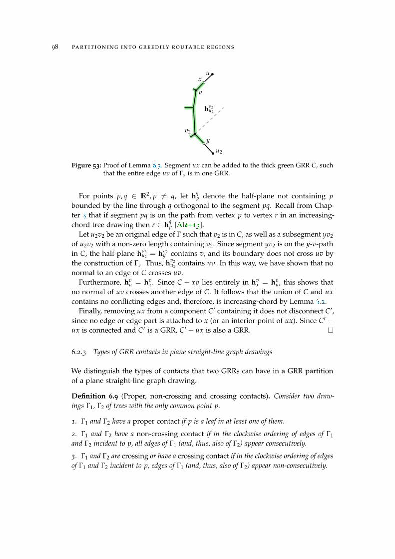
98 partitioning into greedily routable regions

v2

u2

u

v

x

hv2u2

y

Figure 53: Proof of Lemma 6.3

.

. Segment ux can be added to the thick green GRR C, suchthat the entire edge uv of Γs is in one GRR.

For points p, q ∈ R2, p 6= q, let hqp denote the half-plane not containing p

bounded by the line through q orthogonal to the segment pq. Recall from Chap-ter 5

.

that if segment pq is on the path from vertex p to vertex r in an increasing-chord tree drawing then r ∈ hq

p [Ala+13

.

].Let u2v2 be an original edge of Γ such that v2 is in C, as well as a subsegment yv2

of u2v2 with a non-zero length containing v2. Since segment yv2 is on the y-v-pathin C, the half-plane hv2

u2 = hv2y contains v, and its boundary does not cross uv by

the construction of Γs. Thus, hv2u2 contains uv. In this way, we have shown that no

normal to an edge of C crosses uv.Furthermore, hv

u = hvx. Since C − xv lies entirely in hv

x = hvu, this shows that

no normal of uv crosses another edge of C. It follows that the union of C and uxcontains no conflicting edges and, therefore, is increasing-chord by Lemma 6.2

.

.Finally, removing ux from a component C′ containing it does not disconnect C′,

since no edge or edge part is attached to x (or an interior point of ux). Since C′ −ux is connected and C′ is a GRR, C′ − ux is also a GRR.

6.2.3 Types of GRR contacts in plane straight-line graph drawings

We distinguish the types of contacts that two GRRs can have in a GRR partitionof a plane straight-line graph drawing.

Definition 6.9 (Proper, non-crossing and crossing contacts). Consider two draw-ings Γ1, Γ2 of trees with the only common point p.

1. Γ1 and Γ2 have a proper contact if p is a leaf in at least one of them.

2. Γ1 and Γ2 have a non-crossing contact if in the clockwise ordering of edges of Γ1

and Γ2 incident to p, all edges of Γ1 (and, thus, also of Γ2) appear consecutively.

3. Γ1 and Γ2 are crossing or have a crossing contact if in the clockwise ordering of edgesof Γ1 and Γ2 incident to p, edges of Γ1 (and, thus, also of Γ2) appear non-consecutively.

6.3 NP-completeness for graphs with cycles 99

(a) (b) (c)

Figure 54: (a)

.

Proper GRR contact; (b)

.

non-crossing contact which is not proper and(c)

.

crossing contact.

The first part of Definition 6.9

.

allows GRRs to only have contacts as shown inFigure 54a

.

and forbids contacts as shown in Figures 54b

.

, 54c

.

. The second partallows contacts as those in Figure 54b

.

, but forbids the contacts in Figure 54c

.

.Note that a contact of two trees Γ1, Γ2 with a single common point p is either

crossing or non-crossing. Moreover, if the contact of Γ1 and Γ2 is proper, then itis necessarily non-crossing, since for a proper contact, Γ1 or Γ2 has only one edgeincident to p, therefore, all edges of Γ1 and of Γ2 appear consecutively around p.

We shall show that for trees, restricting ourselves to GRR decompositions withonly non-crossing contacts makes the otherwise NP-complete problem of findinga minimum GRR partition solvable in polynomial time.

6.3 NP-completeness for graphs with cycles

We show that finding a minimum decomposition of a plane straight-line draw-ing Γ into increasing-chord trees is NP-hard. This extends the NP-hardness resultby Tan and Kermarrec [TK12

.

] for minimum GRR decompositions of polygonalregions with holes to plane straight-line drawings.

Note that in the graph drawings used for our proof, all GRRs will have propercontacts; see Definition 6.9

.

. Moreover, the graph drawings can be turned into thinpolygonal regions in a natural way by making them slightly “thicker”, and theproof can be reused as another proof for the NP-hardness result in [TK12

.

].Both our NP-hardness proof and the proof in [TK12

.

] are reductions from theNP-complete problem Planar 3SAT [Lic82

.

]. Recall that a Boolean 3SAT formulaϕ is called planar, if the corresponding variable-clause graph Gϕ having a vertexfor each variable and for each clause and an edge for each occurrence of a variable(or its negation) in a clause is a planar graph. In fact, Gϕ can be drawn in the planesuch that all variable vertices are aligned on a vertical line and all clause verticeslie either to the left or to the right of this line and connect to the variables via E-or ∃-shapes [KR92

.

]; see Figure 55

.

.The basic idea of the gadget proof is as follows. Using a number of building

blocks, or gadgets, we construct a plane straight-line drawing Γϕ, whose geometrymimics the variable-clause graph Gϕ drawn as described above. We construct Γϕ

in a way such that its minimum GRR decompositions are in correspondence withthe truth assignments of the Planar 3SAT formula ϕ.

100 partitioning into greedily routable regions

w

x

y

z

c2

c1 c3

Figure 55: An orthogonal graph drawing of the variable-clause graph Gϕ for a planar3SAT formula φ = (w ∨ x ∨ z) ∧ (x ∨ y ∨ z) ∧ (w ∨ x ∨ z).

The variable gadgets in [TK12

.

] are cycles formed by T-shaped polygons whichvariable gadgets

can be made arbitrarily thin. Thus, in the case of plane straight-line drawingswe can use very similar variable gadgets (see Figure 56

.

). The clause gadgetsin [TK12

.

], however, are squares, at which three variable cycles meet. This con-struction cannot be adapted for straight-line plane drawings, and we have toconstruct a significantly different clause gadget; see Figure 58

.

.We define a variable gadget as a cycle of alternating vertical and horizontal

segments. The tip of each segment touches an interior point of the next segment.We can join pairs of consecutive segments into a GRR by assigning each verticalsegment either to the next or to the previous horizontal segment on the cycle.In this way, the variable loop is partitioned either in >-shapes and ⊥-shapes orin a-shapes and `-shapes; see Figure 56

.

.Consider a variable gadget consisting of k T-shapes as shown in Figure 56

.

. Onblack and whitepoints each T-shape we place one black and one white point as shown in the figure. The

points are placed in such a way that neither two black points nor two white pointscan be in one increasing-chord component. Thus, a minimum GRR decompositionof a variable gadget contains at least k components. If it contains exactly k com-ponents, then each component must contain one black and one white point, andthere are exactly two possibilities. Each black point has exactly two white pointsit can share a GRR with, and once one pairing is picked, it fixes all the remainingpairings. The corresponding possibilities are shown in Figure 56a

.

and 56b

.

andwill be used to encode the values true and false, respectively. For the pairing ofthe black and white points corresponding to the true state, the variable loop canbe partitioned in >-shapes and ⊥-shapes, and for the pairing corresponding tothe false state, it can be partitioned in a-shapes and `-shapes.

To pass the truth assignment of a variable to a clause it is part of, we usearm gadgets. Arm gadgets are extensions of the variable gadget. To add an armarm gadgets

gadget to the variable, we substitute several >- or ⊥-shapes from the variable loopby a more complicated structure. Figure 56c

.

shows such extensions for all arm

6.3 NP-completeness for graphs with cycles 101

(a) (b) (c)

Figure 56: Variable gadget and the two possibilities to pair vertical and horizontal seg-ments to make GRRs: (a)

.

true variable state: >-shapes and ⊥-shapes; (b)

.

falsevariable state: a-shapes and `-shapes. (c)

.

Extending the variable gadgets tocreate the upper, middle and lower arm gadgets by substituting T-shapes ofthe variable gadget.

types pointing to the right, the other case is symmetric. In this way, for a variable,we can create as many arms as necessary. Each variable loop will have one armextension for each occurrence of the corresponding variable in a clause in ϕ. Theworking principle for the arm gadgets is the same as for the variable gadgets.The drawing created by the variable cycle and the arm extensions (the variable-arm loop) will once again contain distinguished black and white points, such that variable-arm loop

only one black and one white point can be in a GRR. However, for variable-armloops, the cycles formed by segments of varying orientation are more complicatedthan the loop in Figure 56

.

. For example, for some arm types we use segments ofslopes ±1 in addition to vertical and horizontal segments.

In total twelve variations of the arm gadget will be used, depending on the upper, middle, lowerarmsposition of the literal in the clause, the position of the clause, and whether the

literal is negated or not. Since in Gϕ each clause c connects to three variables,we denote these variables or literals as the upper, middle, and lower variables of cdepending on the order of the three edges incident to c in the one-bend orthogonaldrawing of Gϕ used by Knuth and Raghunathan [KR92

.

]; see Figure 55

.

. Similarly,an arm of c is called an upper, middle, or lower arm if it belongs to a literal of the left and right,

positive andnegative arms

same type in c. An arm is called a right (resp. left) arm if it belongs to a clause thatlies to the right (resp. to the left) of the vertical variable line. Finally, an arm of cis positive if the corresponding literal is positive in c and it is negative otherwise.

102 partitioning into greedily routable regions

qp

b1

b2

b3

w1c

(a)

qp

b1

b2

b3

w1c

(b)

Figure 57: Variable gadget with a right upper positive arm (shaded region). (a)

.

true and(b)

.

false states.

The basic principle of operation of any arm gadget is the same; as an exampleconsider the right upper positive arm in Figure 57

.

. Figures 60

.

, 61

.

, 62

.

and theproof of Property 2

.

cover the remaining arm types.The positive and the negative arms are differentiated by an additional structure

that switches the pairing of the black and white points close to the part of the armthat touches the clause gadget; for example, compare Figures 57b

.

and 62a

.

. By thisinversion, for a fixed truth assignment of the variable, the >- and ⊥-shapes nextto the clause are turned into `- and a-shapes, and vice versa. In this way, theinverted truth assignment of the corresponding variable is passed to the clause.

Note that each arm can be arbitrarily extended both horizontally and verticallyto reach the required point of its clause gadget. We select again black and whitepoints (also called distinguished points) on the line segments of the arm gadget.

The clause gadget (the thickest green polyline in Figure 58

.

, partly drawn inclause gadget

Figure 57

.

) is a polyline which consists of six segments. The first segment hasslope 2, the second is vertical, the third has slope −1, the fourth has slope 1,the fifth is vertical, and the sixth has slope −2. Each clause gadget connects tothe long horizontal segments of the arms of three variable gadgets. The threeconnecting points of the clause gadget are the start and end of the polyline aswell as its center, which is the common point of the two segments with slopes ±1.

We shall prove the following property which is crucial for our construction.

Property 1. 1. Consider a drawing Γi of a variable gadget together with all of its arms.Then, neither two black nor two white points on Γi can be in one GRR. In a minimumGRR decomposition of Γi, each component has one black and one white point, and exactlytwo such pairings of points are possible, one for each truth assignment.

2. Consider two such drawings Γi, Γj for two different variables. Then, no distinguishedpoint of Γi can be in the same GRR as a distinguished point of Γj.

Proof. Part (1) of Property 1

.

extends the same property that we already showedfor variable gadgets without arms to the case including all arms. It is an imme-

6.3 NP-completeness for graphs with cycles 103

upper arm

clause

d

d

cpi

pj

pk

middle arm

lower arm

(a)

c

(b)

Figure 58: Clause gadget (thick green). (a) true and (b) false state of the involved literals.

diate consequence of the way we constructed the arm gadgets and placed thedistinguished points; see Figures 57

.

, 60

.

, 61

.

, 62

.

.Part (2) follows from the way the arms are connected by a clause, i.e., in Fig-

ure 58

.

no pair of points from pi, pj, pk can be in the same GRR, since the threepoints lie on three horizontal segments and are vertically collinear.

The clause gadget is connected to an arm by a horizontal segment with a distin-guished point p on its end, which is either black or white depending on the armtype. Each clause has one special point c chosen as shown in Figure 58

.

.We show that c and p can be in the same GRR in a minimum GRR decomposi-

tion if and only if the variable gadget containing p is in the state that satisfies theclause.

Property 2. 1. In a minimum GRR decomposition, the special point c of a clause gad-get can share a GRR with a black or white point of an arm gadget if and only if thecorresponding literal is in the true state.

2. If a variable assignment satisfies a clause, then its entire clause gadget can be containedin a GRR of an arm corresponding to a true literal.

104 partitioning into greedily routable regions

(a) (b)

Figure 59: Merging the clause gadget with GRRs from the arm loops. (a) None of thethree components is a GRR. (b) All three components are GRRs; see the dashednormals.

Proof. For each arm gadget we select a special red point q; see Figure 57

.

. Point qis neither white nor black. By Property 1

.

, in a minimum GRR decomposition,point q must be in a GRR together with one black and one white point.

For the various arm types, if points q and p are in the same GRR, we shall showthat this GRR cannot contain the entire clause gadget and, in particular, cannotcontain point c. This is illustrated in Figure 59a

.

.Furthermore, we shall show that if the literal is in the true state, then points p

and q are in different GRRs, and the GRR containing p can be merged with theentire clause gadget, including c. For example, in Figure 58a

.

, each variable is in astate that satisfies the clause. The lengths of the thick segments are chosen suchthat each thick blue component can be merged with the clause gadget (thickestgreen) into a single GRR, as shown in Figure 59b

.

.

(i) We first show the lemma for a positive right upper arm. We use the notationfrom Figure 57

.

to refer to the distinguished points. In the true state of the variable(see Figure 57a

.

), points w1, b1 and q are in the same GRR. Points b2 and p arein another GRR (e.g., the thickest green one in Figure 57

.

) which can contain thedistinguished point c of the clause.

In the false state of the variable (see Figure 57b

.

), the points b1 and p are in thesame GRR. Moreover, point q can share a GRR with exactly one point from b1, b2

or b3. But if q were with b2 or b3, then b1 would be disconnected from any whitepoint, a contradiction to the minimality of the decomposition. Thus, points q, b1

and p are in the same GRR, which cannot contain a point of the clause.

(ii) We now show the lemma for a negative right lower arm. We use the notationfrom Figure 60

.

. In the false state of the variable (which corresponds to the truestate of the considered literal), points w1, b1 and q are in the same GRR; seeFigure 60a

.

. Points b2 and p are in another GRR (e.g., the very thick green one in

6.3 NP-completeness for graphs with cycles 105

qp

b1b2

b3

w1

(a)

qp

b1b2

b3

w1

(b)

Figure 60: Right lower negative arm gadget. (a)

.

false and (b)

.

true variable state. Thindashed lines indicate that the variable-arm loop continues.

Figure 57

.

) which can contain the entire clause; see the lower arm in Figure 58

.

andthe corresponding merged component in Figure 59b

.

.Now consider a true state of the variable; see Figure 60b

.

. Point q shares a GRRwith exactly one point from b1, b2 or b3. If q is with b2 or b3, then b1 is disconnectedfrom any white point, a contradiction to the minimality of the decomposition.Thus, points q, b1 and p are in the same GRR, which cannot contain a point of theclause.

(iii) Next, consider a positive right middle arm; see Figure 61

.

. We identifypoints p and b1. Point b1 is either with w0 (true state of the variable) or w1 (falsestate of the variable).

In the true state, points b1 and w0 are in one GRR, which cannot contain q. ThisGRR can be merged with the clause gadget; see Figure 61a

.

, 58

.

and 59b

.

.In the false state, points b1, w1 and q are in one GRR, which cannot contain

point c of the clause.

b1 = p

c

q b2

w1

w2

w0

(a)

b1 = p

c

q b2

w1

w2

w0

(b)

Figure 61: Right positive middle arm gadget. (a)

.

true and (b)

.

false variable state.

106 partitioning into greedily routable regions

(iv) To construct the negative right upper arm, the positive right lower arm andthe negative right middle arm, we invert the arm gadgets constructed before.The inverted gadgets are shown in Figure 62

.

. The proofs are analogous to therespective non-inverted cases.

(v) The left arms are constructed by mirroring.

q

(a)

q

(b)

c

q

(c)

Figure 62: The remaining three right arms in the satisfying variable state. (a)

.

negativeright upper arm, (b)

.

the positive right lower arm and (c)

.

the negative rightmiddle arm.

Finally, we can prove the NP-hardness result by showing that any satisfyingtruth assignment for a formula ϕ yields a GRR decomposition into a fixed num-ber k of GRRs, where k is the total number of black points in our construction.Likewise, using Property 1

.

and 2

.

, we can show that any decomposition into kGRRs necessarily satisfies each clause in ϕ.

Theorem 6.1. For k ∈ N0, deciding whether a plane straight-line drawing can be parti-tioned into k increasing-chord components is NP-complete.

Proof. First, we show that the problem is in NP. Given a plane straight-line draw-ing Γ, we construct its subdivision Γs as described in Section 6.2.2

.

. By Lemma 6.3

.

,it is sufficient to consider only partitions of edges in Γs into k components. To ver-ify a positive instance, we non-deterministically guess the partition of the edgesof Γs into k components. Testing if each component is a tree and if it is increasing-chord can be done in polynomial time.

6.4 trees 107

Next, we show NP-hardness. Given a Planar 3SAT formula ϕ, we construct aplane straight-line drawing Γϕ using the gadgets described above. It is easy tosee that Γϕ can be constructed on an integer grid of polynomial size and in poly-nomial time. Let k be the number of black points produced by the construction.Note that k is O(m + n), where n is the number of variables and m the number ofclauses in ϕ. We claim that Γϕ can be decomposed into k GRRs if and only if ϕ issatisfiable.

Consider a truth assignment of the variables satisfying ϕ. We decompose eachvariable gadget and the attached arms as intended in our gadget design, whichyields exactly k GRRs. By Property 2

.

, each clause gadget can be merged with theGRR of the arm of a literal which satisfies the clause. Therefore, we have k GRRsin total.

Conversely, consider a decomposition of Γϕ into k GRRs. Then, each variableand the attached arms must be decomposed minimally and, by Property 1

.

, mustbe either in the true or in the false state. Furthermore, each special point c ofa clause must be in a component belonging to one of the arms of the clause.But then, the corresponding variable must satisfy the clause by Property 2

.

. Thisinduces a satisfying variable assignment for ϕ.

6.4 trees

In this section we consider greedy tree decompositions, or GTDs. For trees, greedyregions correspond to increasing-chord drawings. Note that increasing-chord treedrawings are either subdivisions of K1,4, subdivisions of the windmill graph (threecaterpillars with maximum degree 3 attached at their “tails”) or paths; see thecharacterization by Alamdari et al. [Ala+13

.

].In the following, we consider a plane straight-line drawing Γ of a tree T =

(V, E), with |V| = n. As before, we identify the tree with its drawing, the ver-tices with the corresponding points and the edges with the corresponding linesegments. We want to partition it into a minimum number of increasing-chordsubdrawings. In such a partition, each pair of components shares at most onepoint.

Recall that a contact of two trees Γ1, Γ2 with a single common point p is eithercrossing or non-crossing; see Definition 6.9

.

. Also, recall that proper contacts arenon-crossing. Let Πall be the set of all GRR partitions of the plane straight-linetree drawing Γ. Let Πnc be the set of GRR partitions of Γ, in which every pair ofGRRs has a non-crossing contact. Finally, let Πp be the set of GRR partitions of Γ,in which every pair of GRRs has a proper contact. It holds: Πp ⊆ Πnc ⊆ Πall.For minimum partitions πp, πnc, πall from Πp, Πnc, Πall, respectively, we have|πall| ≤ |πnc| ≤ |πp|.

We show that finding a minimum GTD of a plane straight-line tree drawing isNP-hard; see Section 6.4.1

.

. In Section 6.4.2

.

, we show that the problem becomespolynomial if we consider GRR partitions in which GRRs have only non-crossing

108 partitioning into greedily routable regions

contacts, i.e., partitions from Πnc. The same holds if we only consider GRR parti-tions in which GRRs only have proper contacts, i.e., partitions from Πp.

6.4.1 NP-completeness

We show that if GRR crossings as in Definition 6.9

.

are allowed, deciding whethera partition of given size exists is NP-complete.

The following problem is known as Partition into Triangles (PIT). It hasbeen shown to be NP-complete by Custic et al. [CKW15

.

, Proposition 5.1] and willbe useful for our hardness proof.

Problem 2 (PIT). Given a tripartite graph G = (V, E) with tripartition V = V1 ∪· V2 ∪·V3, where |V1| = |V2| = |V3| = q. Does there exist a set T of q triples in V1 ×V2 ×V3,such that every vertex in V occurs in exactly one triple and such that every triple inducesa triangle in G?

It is easy to show that the following, similar problem Partition into Indepen-dent Triples (PIIT) is NP-complete as well.

Problem 3 (PIIT). Given a tripartite graph G = (V, E) with tripartition V = V1 ∪· V2 ∪·V3, where |V1| = |V2| = |V3| = q. Does there exist a set T of q triples in V1 ×V2 ×V3,such that every vertex in V occurs in exactly one triple and such that no two vertices of atriple are connected by an edge in G?

Lemma 6.4. PIIT is NP-complete.

Proof. It is easy to see that PIIT is in NP. For NP-hardness, consider a graph G =

(V, E) from an instance of PIT. We construct G′ = (V, E′) with E′ = uv | uv 6∈E, u ∈ Vi, v ∈ Vj, i 6= j for i, j = 1, 2, 3. In this way, a triple from V1 × V2 × V3

induces a triangle in G if and only if it is independent in G′. Therefore, PIT canbe reduced to PIIT in polynomial time.

We now show that deciding whether a GRR partition of a plane straight-linetree drawing of given size exists is NP-complete even for subdivisions of a star.

Theorem 6.2. Given a plane straight-line drawing Γ of a tree T = (V, E), which isa subdivision of a star with 3q leaves, it is NP-complete to decide whether Γ can bepartitioned into q GRRs.

Proof. The proof that the problem is in NP is analogous to the correspondingproof of Theorem 6.1

.

.To prove NP-hardness, we present a polynomial-time reduction from PIIT. Con-

sider the tripartite graph G = (V, E) with tripartition V = V1 ∪· V2 ∪· V3 from aninstance Π = (G, V1, V2, V3, q) of PIIT, where |V1| = |V2| = |V3| = q. We mayassume q ≥ 3. We show how to construct a plane straight-line drawing Γ of asubdivision of a star in polynomial time, such that Γ can be partitioned into qGRRs if and only if Π is a yes-instance of PIIT. Figure 63

.

shows an example ofsuch a construction for q = 3.

6.4 trees 109

o

vΓ1

vΓ2

vΓ3

uΓi

wΓi

o

magnified

magnified

magnified

uΓ1 uΓ

2 uΓ3

Figure 63: Reduction from a PIIT instance with q = 3 for the proof of Theorem 6.2

.

.

We use the following basic ideas to construct the drawing Γ. Let o be thecenter of Γ. Each vertex v of G corresponds to a leaf vertex vΓ of Γ. The leavesof Γ are partitioned into three sets corresponding to V1, V2, V3. Consider a pair ofvertices u ∈ Vi, v ∈ Vj. If i = j, the angle that the uΓ-vΓ-path has at point o inour construction is at most 12. Therefore, u and v can not be in the same GRR.For i 6= j, however, the angle that the uΓ-vΓ-path has at point o is between 106

and 134. We construct the o-uΓ and o-vΓ paths in such a way that the uΓ-vΓ-pathis increasing-chord if and only if edge uv is not in G.

The path from o to vΓ takes a left turn of at most 12 and then continues as astraight line, except for at most q dents; see the left magnified part of Figure 63

.

.Each dent is used to realize exactly one edge from G. For a pair of vertices u ∈ Vi,v ∈ Vj, j ≡ i + 1 (mod 3) with edge uv in G, the o-uΓ-path has a dent with anormal crossing the o-vΓ-path. Furthermore, no normal to this dent crosses the o-wΓ-path for any vertex w ∈ Vj ∪ Vk \ v, for k ≡ i + 2 (mod 3). Consider theexample in Figure 63

.

. Assume that there is an edge u3v2 in G. Then, the o-uΓ3 -

110 partitioning into greedily routable regions

q

c1 · q

c2 · q2

2q

2q− 1

q + 1

uΓ0

uΓ1

uΓ2

uΓq

uΓq+1q

...

o

(a)

vΓ1vΓ

2vΓ3vΓ

4vΓ5

vΓ0

vΓ2

vΓ3

vΓ4

(b)

Figure 64: Constructing Γ from Π for the proof of Theorem 6.2

.

. (a)

.

Choosing coordinatesfor points o, uΓ

0 , . . . , uΓq+1. (b)

.

Determining dent positions on the o-uΓi -paths.

path has a dent whose normal (dashed red) crosses the o-vΓ2 -path, but not the

paths from o to vΓ1 , vΓ

3 , wΓ1 , wΓ

2 and wΓ3 .

We now describe the procedure to construct Γ from Π in detail. We will makesure that all vertices of Γ have rational coordinates with numerators and denom-inators in O(n2). Let V1 = u1, . . . , uq, V2 = v1, . . . , vq and V3 = w1, . . . , wq.For the construction, we introduce dummy points uΓ

0 , uΓq+1, vΓ

0 , vΓq+1, wΓ

0 , wΓq+1,

which do not lie on Γ. For all i = 0, . . . , q + 1, we shall have |ouΓi | = |ovΓ

i | = |owΓi |.

We first show how to choose coordinates for points o, uΓ0 , . . . , uΓ

q+1; see Fig-ure 64a

.

. We approximate 120 rotation using the angle α ≈ 120.51 with cos α =

− 3365 and sin α = 56

65 . The points vΓi are acquired from uΓ

i by a clockwise rotationby α at o, and the points wΓ

i are acquired from uΓi by a counterclockwise rotation

by α at o. Then, ∠uΓi ovΓ

i = ∠uΓi owΓ

i = α and ∠vΓi owΓ

i = 360 − 2α ≈ 118.98.Let point o have coordinates (0, 0). For i = 1, . . . , q, let the first segment of the o-

uΓi -path have its other endpoint in (i, c1q) for a constant c1. For i = 0, . . . , i + 1,

point uΓi has x-coordinate i. Let yi denote the y-coordinate of uΓ

i . We set y0 =

c1q + c2q2 for a constant c2. For i = 1, . . . , q, we set yi = yi−1 + 2q + 1− i; seeFigure 64a

.

. Thus, for i = 0, . . . , q + 1, points uΓi lie on a parabola that opens down.

Note that all vertices of Γ constructed so far are integers in O(n2). We set c1 = 5and c2 = 40.

6.4 trees 111

12

1

52

(a) (b)

Figure 65: Proof of Theorem 6.2

.

continued. (a)

.

Constructing dents on the o-uΓi -paths.

(b)

.

All dents lie inside the three dark gray regions.

Next, we show how to construct the dents on the o-uΓi -paths. For edge uivj

in G, i, j = 1, . . . , q, consider the straight line through vΓj−1vΓ

j+1; see the dashed redline in Figure 64b

.

for j = 3. Consider the intersection of this line and the verticalline through uΓ

i . The coordinates of that intersection are rational numbers withnumerators and denominators in O(n2). It is easy to show that this intersectionhas y-coordinates between 20q and 80q.

At the intersection, we place a dent consisting of two segments; see Figure 65a

.

.The first segment of the dent has positive slope and is orthogonal to vΓ

j−1vΓj+1. Its

projection on the x axis has length 12 . The second segment has the negative slope

of −5. It is easy to verify that the line through vΓj vΓ

j+2 (the upper red dashedline in Figure 65a

.

) has distance at least c28 = 5 from the lowest point of the dent.

Therefore, the dent fits between the two dashed red lines. Note that all threevertices of the dent have coordinates that are rational numbers with numeratorsand denominators in O(n2).

By the choice of the slopes, no normal to either one of the two dent segmentscrosses owΓ

k for k = 0, . . . , q + 1. Furthermore, no normal on the second segmentcrosses ovΓ

k for k = 0, . . . , q + 1, and a normal to the first segment only crosses ovΓk

for k = j. In this way, the dent ensures that uΓi and vΓ

j can not be in the same GRR,and it does not prohibit any other vertex pair (uΓ

k and vΓ` , vΓ

k and wΓ` , wΓ

k and vΓ` ,

for k, ` = 1, . . . , q) from being in the same GRR. Finally, for each leaf vertex uΓi , we

add the missing segments on the vertical line through uΓi to connect o and uΓ

i bya path. Analogously, we construct the o-vΓ

i - and the o-wΓi -paths.

Note that by our construction, the dent normals do not cross other dents on thepaths from o to the leaves from another partition; see Figure 65b

.

, where the dents

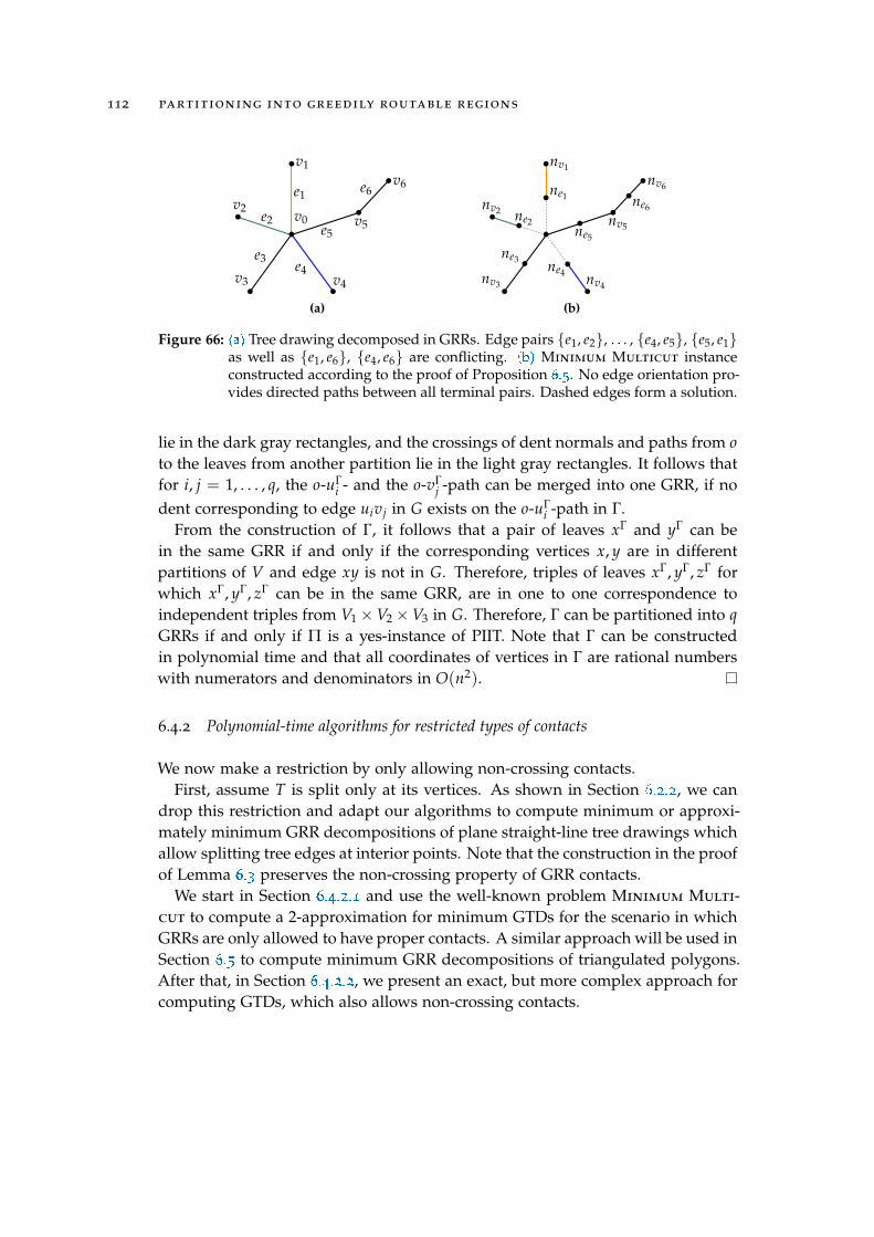
112 partitioning into greedily routable regions

v0

v1

v2

v3 v4

v5

v6e1

e2

e3 e4

e5

e6

(a)

nv1

nv2

nv3 nv4

nv5

nv6ne1

ne2

ne3 ne4

ne5

ne6

(b)

Figure 66: (a)

.

Tree drawing decomposed in GRRs. Edge pairs e1, e2, . . . , e4, e5, e5, e1as well as e1, e6, e4, e6 are conflicting. (b)

.

Minimum Multicut instanceconstructed according to the proof of Proposition 6.5

.

. No edge orientation pro-vides directed paths between all terminal pairs. Dashed edges form a solution.

lie in the dark gray rectangles, and the crossings of dent normals and paths from oto the leaves from another partition lie in the light gray rectangles. It follows thatfor i, j = 1, . . . , q, the o-uΓ

i - and the o-vΓj -path can be merged into one GRR, if no

dent corresponding to edge uivj in G exists on the o-uΓi -path in Γ.

From the construction of Γ, it follows that a pair of leaves xΓ and yΓ can bein the same GRR if and only if the corresponding vertices x, y are in differentpartitions of V and edge xy is not in G. Therefore, triples of leaves xΓ, yΓ, zΓ forwhich xΓ, yΓ, zΓ can be in the same GRR, are in one to one correspondence toindependent triples from V1×V2×V3 in G. Therefore, Γ can be partitioned into qGRRs if and only if Π is a yes-instance of PIIT. Note that Γ can be constructedin polynomial time and that all coordinates of vertices in Γ are rational numberswith numerators and denominators in O(n2).

6.4.2 Polynomial-time algorithms for restricted types of contacts

We now make a restriction by only allowing non-crossing contacts.First, assume T is split only at its vertices. As shown in Section 6.2.2

.

, we candrop this restriction and adapt our algorithms to compute minimum or approxi-mately minimum GRR decompositions of plane straight-line tree drawings whichallow splitting tree edges at interior points. Note that the construction in the proofof Lemma 6.3

.

preserves the non-crossing property of GRR contacts.We start in Section 6.4.2.1

.

and use the well-known problem Minimum Multi-cut to compute a 2-approximation for minimum GTDs for the scenario in whichGRRs are only allowed to have proper contacts. A similar approach will be used inSection 6.5

.

to compute minimum GRR decompositions of triangulated polygons.After that, in Section 6.4.2.2

.

, we present an exact, but more complex approach forcomputing GTDs, which also allows non-crossing contacts.

6.4 trees 113

6.4.2.1 2-approximation using Multicut

We show how to partition the edges of T into a minimum number of increasing-chord components with proper contacts using Minimum Multicut on trees. For Minimum

Multicuta given edge-weighted graph G = (V, E) and a set of terminal pairs (s1, t1), . . . ,(sk, tk), an edge set S ⊆ E is a multicut if removing S from G disconnects eachpair si, ti, i = 1, . . . , k. A multicut is minimum if the total weight of its edges isminimum.

For the complexity of Minimum Multicut on special graph types, see the sur-vey by Costa et al. [CLR05

.

]. Computing Minimum Multicut is NP-hard even forunweighted binary trees [CFR03

.

], but has a polynomial-time 2-approximation fortrees [GVY97

.

].Consider a plane straight-line drawing of a tree T = (V, E). We construct a

tree TM by subdividing every edge of T once as follows. Tree TM has a vertex nv

for each vertex v ∈ V and a vertex ne for each edge e ∈ E. For each e = uv ∈ E,edges nune and nenv are in TM. The set X of terminal pairs contains a pair (ne, n f )

for each pair of conflicting edges e, f of T. Let all edges of TM have weight 1.

Lemma 6.5. Let E′ be a Minimum Multicut of TM with respect to the terminalpairs X and let CM

1 , . . . , CMk denote the connected components of TM − E′. Then, compo-

nents Ci = e ∈ E | ne ∈ CMi form a minimum GRR decomposition of T with proper

contacts.

Proof. Consider a multicut E′ of TM, |E′| = k− 1. Consider a connected compo-nent CM

i of TM − E′. Then, the edges in Ci = e ∈ E | ne ∈ CMi are conflict-free

and form a connected subtree Ti of T. Thus, Ti is a GRR by Lemma 6.2

.

. It is easyto see that such GRRs have proper contacts. Consider a vertex v ∈ V and edges e,f , g, h ∈ E, each incident to v, such that e and f are in one GRR and g and h inanother. But then, ne and n f are in one connected component of TM − E′ and ng

and nh in another, a contradiction.Next, consider a GRR decomposition of T into k subtrees Ti = (Vi, Ei) with

proper contacts. We create an edge set S iteratively as follows. Assume Ti, Tj

touch at vertex v ∈ V. Let edge e = uv be in Ti, and let v be a leaf in Ti. We thenadd edge nenv of TM to set S, as long as the number of connected componentsin TM− S increases by one; see Figure 66a

.

and 66b

.

. In the end, we have |S| = k− 1.After removing S from TM, no connected component contains vertices ne1 , ne2 fora pair of conflicting edges e1, e2. Thus, S is a multicut.

We have shown that GRR decompositions of T with proper contacts and size kare in one-to-one correspondence with the multicuts of TM of size k− 1. Therefore,minimum multicuts correspond to minimum GRR decompositions, and it followsthat Ci form a minimum GRR decomposition of T with proper contacts.

Note that Minimum Multicut can be solved in polynomial time in directedtrees [CLR03

.

], i.e., trees whose edges can be directed such that for each terminalpair (si, ti), the si-ti-path is directed. We note that this result cannot be applied in

114 partitioning into greedily routable regions

our context, since we can get Minimum Multicut instances for which no such ori-entation is possible, see Figure 66b

.

. However, using the approximation algorithmfrom [GVY97

.

], we obtain the following result.

Corollary 6.1. Given a plane straight-line drawing of a tree T = (V, E), a partitionof E into 2 ·OPT− 1 increasing-chord subtrees of T having only proper contacts can becomputed in time polynomial in n, where OPT is the minimum size of such a partition.

6.4.2.2 Optimal solution

In the following we show how to find a minimum GRR partition with only non-crossing contacts in polynomial time. As is the case with minimum partitionsof simple hole-free polygons into convex [CD85

.

] or star-shaped [Kei85

.

] compo-nents, our algorithm is based on dynamic programming. We describe the dy-namic program in detail and use it to find minimum GTDs for the setting as inSection 6.4.2.1

.

, as well as for the setting in which non-proper, but non-crossingcontacts of GRRs are allowed. First, we shall prove the following theorem.

Theorem 6.3. Given a plane straight-line drawing of a tree T = (V, E), a partition of Einto a minimum number of increasing-chord subtrees of T (minimum GTD) having onlynon-crossing contacts can be computed in time O(n6).

At the end of Section 6.4.2.2

.

, we modify our dynamic program slightly to proveTheorem 6.4

.

, which shows the same result for the setting in which only partitionswith proper contacts are considered.

Theorem 6.4. Given a plane straight-line drawing of a tree T = (V, E), a partition of Einto a minimum number of increasing-chord subtrees of T (minimum GTD) having onlyproper contacts can be computed in time O(n6).

Let T be rooted. For each vertex u with parent πu, let Tu be the subtree of usubtree Tu

together with edge πuu. We shall use the following definition.

Definition 6.10 (root component). Given a GRR partition of the edges of a rootedtree T′, we call all GRRs containing the root of T′ the root components. If the root of T′root component

has degree 1, every GRR partition of T′ has one unique root component.

A minimum partition is constructed from the solutions of subinstances as fol-lows. Let u1, . . . , ud be the children of u. For subtrees Tu1 , . . . , Tud whose onlycommon vertex is u, a minimum partition P′ of T′ =

⋃i Tui induces partitions Pi

of Tui . Furthermore, P′ is created by choosing Pi as partitions of Tui and possiblymerging some of the root components of Tui , i = 1, . . . , d. Note that Pi is not neces-sarily a minimum partition of Tui , if Pi allows us to merge more root componentsthan a minimum partition of Tui would allow. Therefore, for every u we shallstore minimum partitions of Tu for various possibilities of the root componentof Tu. For the sake of uniformity, we choose a vertex with degree 1 as the rootof T.

6.4 trees 115

r

ρ1

ρ2

ρ3

t1t3t2

(a)

ru1

v1

u4v4

ρ1

ρ2

ρ3

ρ4

(b)

Figure 67: (a)

.

Path ρ2 is clockwise between paths ρ1 and ρ3. (b)

.

Statement of Lemma 6.6

.

.

Given a tree root, the number of different subtrees it could be contained in maybe exponential, e.g., it is Θ(2n) in a star. The key observation for our algorithmis that we do not need to store a partition for each possible root component. Werequire the following notation.

Definition 6.11 (Path clockwise between). Consider directed non-crossing paths ρ1,ρ2, ρ3 with common origin r, endpoints t1, t2, t3 and, possibly, common prefixes. Let Vi

be vertices of ρi, i = 1, 2, 3, and let T be the tree formed by the union of ρ1, ρ2 and ρ3. Wesay that ρ2 is clockwise between ρ1 and ρ3, if the clockwise traversal of the outer faceof T visits t1, t2, t3 in this order; see Figure 67a

.

.

Note that in Definition 6.11

.

the three paths may (partially) coincide. Lemma 6.6

.

shows that to decide whether a union of two subtrees is increasing-chord, it issufficient to consider only the two pairs of “outermost” root-leaf paths of eachsubtree. This result is crucial for limiting the number of representative decompo-sitions that need to be considered during our dynamic programming approach.The statement of the lemma is illustrated in Figure 67b

.

.

Lemma 6.6. Let T1, T2 be increasing-chord trees sharing a single vertex r. Let all treeedges be directed away from r. Let paths ρ1, ρ2 in T1 and ρ3, ρ4 in T2 be paths from r toa leaf, such that:

- every directed path from r in T1 is clockwise between ρ1 and ρ2;- every directed path from r in T2 is clockwise between ρ3 and ρ4;- for i = 1, . . . , 4, path ρi is clockwise between ρi−1 and ρi+1 (indices modulo 4).

Then, ρ1 ∪ ρ2 ∪ ρ3 ∪ ρ4 is increasing-chord if and only if T1 ∪ T2 is increasing-chord.

Proof. Consider trees T1, T2 and paths ρ1, . . . , ρ4 satisfying the condition of thelemma; see Figure 67b

.

for a sketch. Note that ρ1 and ρ2 may have commonprefixes, and so may ρ3 and ρ4. Assume the four paths ρ1, . . . , ρ4 are drawn withincreasing chords, but the union T′ of the trees T1 and T2 is not. Then, without lossof generality, there exist edges u1v1 in T1 and u4v4 in T2, such that the normal `to u1v1 at u1 crosses edge u4v4.

As defined in Chapter 3

.

, we say that an edge uv points upwards, downwards etc.

116 partitioning into greedily routable regions

u1

v1

r

u4

v4

ρ2ρ3

ρ′ ρ′′

v2

u2

v3

u3

(a)

v2

v3

u3

u1

v1

r

u4

v4

ρ2

ρ3 `3

u2

(b)

Figure 68: Constructions in the proof of Lemma 6.6

.

.

Claim 2. Without loss of generality, we may assume the following; see Figure 68

.

.

(i) Edge u1v1 points vertically upwards,

(ii) edge u4v4 is the first edge on the r-v4 path ρ′′ crossed by ` and points upwards,

(iii) vertex u4 is on ` and to the right of u1.

We ensure (i) by rotation. Then, point r is below ` (or on it), since the r-v1-path ρ′ is increasing-chord. For (ii), we choose u4v4 as the first edge with thisproperty. If it points downward, there is an edge on the r-u4-path crossed by `.For (iii), if ` crosses u4v4 in an interior point p, we subdivide the edge at p andreplace u4v4 by pv4. If u4 is left of u1, we mirror the drawing horizontally. Thisproves the claim.

First, assume that v1, v4 are not on paths ρ1, . . . , ρ4. Recall that two of thepaths ρ1, . . . , ρ4 (without loss of generality, ρ2 and ρ3) are between ρ′ and ρ′′. Letu2v2 and u3v3 be the last two edges on ρ2 and ρ3, respectively. Note that ray(u1, v1)

and ray(u2, v2) must diverge, and so must ray(u2, v2) and ray(u3, v3). If u4v4

points upwards and to the left as in Figure 68a

.

, then ray(u3, v3) and ray(u4, v4)

must converge; a contradiction. Thus, u2v2, u3v3 and u4v4 point upwards andto the right; see Figure 68b

.

. Since T1 as well as the union of ρ1 and ρ2 areincreasing-chord, the angles ∠v1u1u2, ∠u1u2v2, ∠v2u2u3 and ∠u2u3v3 are be-tween 90 and 180. Therefore, vertices u2 and u3 must lie below `. Let `3 bethe normal to u3v3 at u3. Since T2 is drawn with increasing chords, u4v4 must liebelow `3, a contradiction.

The proof works similarly if u1v1 is on ρ2 (by identifying u1v1 and u2v2), andthe remaining cases are symmetric.

We now describe our dynamic programs for proper and non-crossing contactsin detail. We first give an overview of the general approach, then describe thenon-crossing case and afterwards modify it for proper contacts. For a root com-leftmost and

rightmost paths ponent R of Tu, let the leftmost path (or, respectively, the rightmost path) be thesimple path in R starting at πu which always chooses the next counterclockwise(clockwise) edge.

6.4 trees 117

The basic idea of the dynamic program is as follows. For a given subtree Tu, westore the sizes of the minimum GTDs of Tu for different possibilities of the rootcomponent. We combine these solutions to compute minimum GTDs of biggersubtrees. For this step, we must be able to test which root components can bemerged into one GRR. Instead of storing the partition sizes for all possible rootcomponents, we only store the minimum partition size for each combination ofthe leftmost and rightmost path of the root component. Thus, for each Tu, weonly store O(n2) partition sizes. Note that this is sufficient, since by Lemma 6.6

.

the question whether two root components can be merged depends only on theirleftmost and rightmost paths.

If u is the root of a subtree T′ and has degree 2 or greater in T′, there mightbe several root components in a partition of T′, i.e., GRRs containing u. Let R besome fixed root component of the considered GTD. If u has degree 2 or greaterin R, then we need a reference direction to define the leftmost and rightmost pathsof R. Let ρl be the leftmost path of the rooted tree R + πuu. Note that ρl containsthe edge πuu. Then, the leftmost path of R is ρl − πuu. The rightmost path of Ris defined analogously.

Recall that Tu is the subtree of u together with edge πuu. For each pair of table τ

vertices ti, tj in Tu, cell τ[u, ti, tj] of a table τ stores the size of a minimum GRR values τ[u, ti, tj]

decomposition of Tu, in which the root component has the πu-ti-path and the πu-tj-path as its leftmost and rightmost path, respectively. Cell τ[u] stores the sizeof a minimum GRR decomposition of Tu. We have τ[u] = minti ,tj τ[u, ti, tj]. Forsimplicity, we set min ∅ = ∞.

Clearly, for each leaf u, τ[u, u, u] = 1, and τ[u, ti, tj] = ∞ for all other valuesof ti, tj. Let v be the only neighbor of the root r of the tree T. Then, τ[v] is the sizeof a minimum GRR decomposition of T. We show how to compute τ bottom-up.

For ease of presentation, we use the following notation. Vertex u is not a leafand has children u1, . . . , ud. Let πu, u1, . . . , ud have this clockwise order around u.Let ti 6= u be a vertex in Tui . We define tj, tk, t` analogously for 1 ≤ i ≤ j ≤ k ≤` ≤ d. Let ρi be the u-ti-path.

We consider two settings: allowing arbitrary non-crossing contacts and allow-ing only proper contacts. The dynamic programs for the two cases are very simi-lar, and the program for arbitrary non-crossing contacts is slightly more complex.To reduce duplication, we first present the program for arbitrary non-crossingcontacts, and later show how to modify it for the case when only proper contactsare allowed.

6.4.2.3 Non-crossing contacts

Recall that vertex u can live in a root component R together with non-consecutivechildren ui, u`, i < `. If arbitrary non-crossing contacts are allowed, some nodesfrom ui+1, . . . , u`−1 that are not in R can also be in one GRR. Therefore, afterchoosing the root component R of Tu, we must be able to recursively compute the

118 partitioning into greedily routable regions

minimum size of a partition of the union of Tuj , uj /∈ R. We introduce additionaltables for this purpose.

In addition to the table τ storing the values τ[u, ti, tj], we use tables σ∆ for ∆ =

1, . . . , 4, as well as tables σ and σM. These additional tables will be used to for-tables σ∆, σ, σM

mulate the recurrences for τ. For fixed u, i, j, the corresponding values of σ∆, σ

and σM denote the sizes of minimum GTDs of Tui ∪ Tui+1 ∪ · · · ∪ Tuj with certainproperties. Table σ∆ considers different possibilities of the leftmost and rightmostpaths of the root components as well as the degree ∆ of u in the root component.Recall that in an increasing-chord tree drawing, every vertex has degree at most 4.Formally, the value σ∆[u, ti, tj] denotes the minimum number of GRRs in a GTDσ∆[u, ti, tj]

of the tree Tui ∪ Tui+1 ∪ · · · ∪ Tuj , in which there exists a GRR R with the rightmostpath u-ti and leftmost path u-tj and in which u has degree ∆ in R.

For some recurrences, we need to aggregate the various possibilities storedin σ∆. For this purpose, we use tables σ and σM as follows. The value σ isσ[u, ti, tj]

the minimum of σ∆ over all values of ∆. We define σ[u, ti, tj] as σ[u, ti, tj] =

min∆=1,...,4 σ∆[u, ti, tj].The value σM stores the minimum over all combinations of the leftmost and

rightmost paths. Thus, it stores the size of the minimum partition of Tui ∪ · · · ∪Tuj , regardless of the root component. Formally, σM[u, i, j] denotes the minimumσM[u, i, j]

number of GRRs in a GTD of Tui ∪ · · · ∪ Tuj . Note that the arguments of σM[u, ·, ·]are indices i, j of a pair of children of u, and the arguments of σ∆[u, ·, ·] and σ[u, ·, ·]are a pair of vertices in Tui ∪ · · · ∪ Tuj .

In the following recurrences, for a fixed pair of vertices ti and t`, all possibil-ities for tj and tk are considered, such that both paths ρj and ρk are clockwisebetween ρi and ρ`. We test whether root components R1 with the leftmost andrightmost paths ρi and ρj and R2 with the leftmost and rightmost paths ρk and ρ`can be merged to a single GRR. We show that this covers all representative possi-bilities for a root component of a GTD of Tui ∪ · · · ∪ Tu`

to have the leftmost andrightmost paths ρi and ρ`, respectively.

Lemma 6.7. We have the recurrences

(1) σ1[u, ti, tj] = σ[u, ti, tj] = τ[ui, ti, tj] for all ti, tj 6= u in Tui , i = 1, . . . , d;

(2) σM[u, i, i] = τ[ui] for all i = 1, . . . , d;

(3) σ2[u, ti, t`] = mintj,tkσ1[u, ti, tj] + σM[u, j + 1, k− 1] + σ1[u, tk, t`]− 1;(4) σ3[u, ti, t`] = minmin

tj,tkσ2[u, ti, tj] + σM[u, j + 1, k− 1] + σ1[u, tk, t`]− 1,

mintj,tkσ1[u, ti, tj] + σM[u, j + 1, k− 1] + σ2[u, tk, t`]− 1;

(5) σ4[u, ti, t`] = mintj,tk σ1[u, ti, ti] + σM[u, i + 1, j− 1]

+σ1[u, tj, tj] + σM[u, j + 1, k− 1]

+σ1[u, tk, tk] + σM[u, k + 1, `− 1]

+σ1[u, t`, t`] − 3.

6.4 trees 119

πu

uui= uj

uk= u`

Tuj+1 Tuk−1· · ·

tk

t`

tj

ti

(a)πu

uui

uj

uk= u`

Tuj+1

Tuk−1

···

tk

t`

tj

ti

(b)πu

u

uk

u`

Tuk−1

··· tk

t`ui= uj

tj

ti

Tuj+1

(c)

Figure 69: Recurrences in Lemma 6.7

.

: (a)

.

recurrence (3

.

); (b)

.

recurrence (4

.

) for thecase m = j; (b)

.

recurrence (4

.

) for the case m = k.

The minimizations in recurrences (3

.

), (4

.

) and (5

.

) only consider vertices tj, tk, such thatthe subtree ρi ∪ ρj ∪ ρk ∪ ρ` is increasing-chord.

Proof. Consider recurrence (1

.

). First, we prove σ1[u, ti, tj] = τ[ui, ti, tj] as follows.For a GTD from the definition of σ1[u, ti, tj] we show that its size is an upperbound for τ[ui, ti, tj]. Then, for a GTD from the definition of τ[ui, ti, tj], we showthat its size is an upper bound for σ1[u, ti, tj].

Consider a GTD of Tui ∪ · · · ∪ Tuj of size x with root component R, such that Rhas u-ti and u-tj as its leftmost and rightmost paths, respectively. Since u hasdegree 1 in R, we have i = j. Thus, this partition is a GTD of Tui with R as theroot component, so by definition of τ we have τ[ui, ti, tj] ≤ x. Thus, we haveσ1[u, ti, tj] ≥ τ[ui, ti, tj]. Conversely, consider a GTD of Tui , such that its rootcomponent R has u-ti and u-tj as its leftmost and rightmost paths. Thus, ti and tj

are both in Tui , and vertex u has degree 1 in R. By the definition of σ1, thispartition has size at least σ1[u, ti, tj]. Thus, we have σ1[u, ti, tj] ≤ τ[ui, ti, tj]. Finally,since for i = j we have Tui ∪ · · · ∪ Tuj = Tui , vertex u can only have degree 1 in theroot component of a GTD, so we have σ1[u, ti, tj] = σ[u, ti, tj]. Thus, recurrence (1

.

)holds.

Recurrence (2

.

) holds trivially, since by the definitions of σM and τ[·], bothσM[u, i, i] and τ[ui] denote the size of the minimum GRR partition of Tui .

Consider recurrence (3

.

) and a GTD P of Tui ∪ · · · ∪ Tu`of size x with root com-

ponent R. Again, let R have u-ti and u-t` as its leftmost and rightmost paths,respectively. Let u have degree 2 in R. Therefore, i 6= `, and R only consistsof two parts R1, R2 (green and blue in Figure 69a

.

, respectively), such that R1 iscontained in Tui and R2 is contained in Tu`

. Partition P induces a GTD P1 of Tui

of size x1, a GTD P2 of Tu`of size x2 and a GTD P3 of Tui+1 ∪ · · · ∪ Tu`−1 of size x3.

Since R1 ∪ R2 = R, we have x = x1 + x2 + x3 − 1. Let uj be a vertex in R1, suchthat u-uj is the rightmost path of R1. Let uk be the vertex in R2, such that u-uk isthe leftmost path of R2. The subtree ρi ∪ ρj ∪ ρk ∪ ρ` is contained in R and, there-fore, is increasing-chord. By the definition of σ1 and σM, we have σ1[u, ti, tj] ≤ x1,σ1[u, tk, t`] ≤ x2 and σM[u, j + 1, k− 1] ≤ x3. Thus, the right part of recurrence (3

.

)is at most x, so the right side is upper bounded by the left side.

120 partitioning into greedily routable regions

Conversely, let the right side of recurrence (3

.

) be less than ∞. Let j, k, tj, tk bechosen such that the minimum on the right side is realized. Then, ρi ∪ ρj ∪ ρk ∪ ρ`is increasing-chord. Let σ1[u, ti, tj] = x1, and let P1 be a GTD of size x1 realizingthe minimum in the definition of σ1[u, ti, tj]. Let R1 be the root component of P1.Then, R1 has leftmost and rightmost paths u-ti and u-tj respectively. Analogously,let σ1[u, tk, t`] = x2, and let P2 be a GTD of size x2 realizing the minimum inthe definition of σ1[u, tk, t`]. Let R2 be the root component of P2. Then, R2 hasleftmost and rightmost paths u-tk and u-t` respectively. Finally, let P3 be a GTD ofsize x3 realizing the minimum in the definition of σM[u, j+ 1, k− 1]. By Lemma 6.6

.

,R1∪R2 is increasing-chord. Consider the GTD P formed by taking the union of P1,P2 and P3 and merging R1 and R2. Partition P has size x1 + x2 + x3 − 1. Its rootcomponent R has leftmost and rightmost paths u-ti and u-t` respectively, and uhas degree 2 in R. Thus, by the definition of σ2[u, ti, t`], we have σ2[u, ti, t`] ≤x1 + x2 + x3− 1. Thus, the left side of recurrence (3

.

) is upper bounded by its rightside. Therefore, recurrence (3

.

) holds.

Next, consider recurrence (4

.

) and a GRR partition P of Tui ∪ · · · ∪ Tu`of size x

with root component R. Once again, let R have u-ti and u-t` as its leftmost andrightmost paths, respectively. Let u have degree 3 in R. Therefore, i 6= `. Inaddition to ui and u`, the GRR R must contain another child um of u, such that i <m < `. We can partition R into two GRRs R1 and R2, such that ui is in R1, u` in R2

and um is either in R1 or in R2. First, assume um is in R1; see Figure 69b

.

. Theother case is symmetric; see Figure 69c

.

. We choose j = m. Let tj be a vertexin Tuj , such that u-tj is the rightmost path of R1. Let tk be a vertex in Tu`

, suchthat u-tk is the leftmost path in R2. Note that in this case, tk and t` are in thesame subtree Tuk = Tu`

. We can split the partition P into GRR partitions P1

of Tui ∪ · · · ∪ Tuj of size x1, P2 of Tu`of size x2 and P3 of Tuj+1 ∪ · · · ∪ Tuk−1 of

size x3. It holds: R = R1 ∪ R2, and apart from R, no other GRR in P is split,since the contacts are non-crossing. Thus, x = x1 + x2 + x3 − 1. By definition,σ2[u, ti, tj] ≤ x1, σ1[u, tk, t`] ≤ x2 and σM[u, j + 1, k− 1] ≤ x3. Therefore, the rightside of recurrence (4

.

) is at most x. The same holds for the symmetric case inwhich um is in R2 by analogous arguments. Thus, the right side of recurrence (4

.

)is upper bounded by its left side.

Conversely, let the right side of recurrence (4

.

) be less than ∞. Let j, k, tj, tk bechosen such that the minimum on the right side is realized. First, assume it isrealized by σ2[u, ti, tj] + σM[u, j + 1, k− 1] + σ1[u, tk, t`]− 1. Then, ρi ∪ ρj ∪ ρk ∪ ρ`is increasing-chord. Let σ2[u, ti, tj] = x1, and let P1 be a GRR partition of size x1 re-alizing the minimum in the definition of σ2[u, ti, tj]. Let R1 be the root componentof P1. Then, R1 has leftmost and rightmost paths u-ti and u-tj respectively. Thedegree of u in R1 is 2, and the vertices ti and tj must lie in different subtrees Tui

and Tuj , respectively. Analogously, let σ1[u, tk, t`] = x2, and let P2 be a GRR parti-tion of size x2 realizing the minimum in the definition of σ1[u, tk, t`]. Let R2 be theroot component of P2. Then, R2 has leftmost and rightmost paths u-tk and u-t`respectively. Finally, let P3 be a GRR partition of size x3 realizing the minimumin the definition of σM[u, j + 1, k− 1]. By Lemma 6.6

.

, R1 ∪ R2 is increasing-chord.

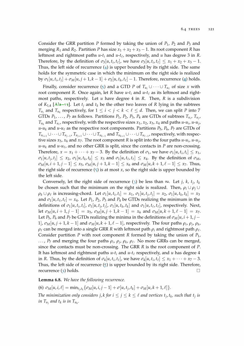
6.4 trees 121

Consider the GRR partition P formed by taking the union of P1, P2 and P3 andmerging R1 and R2. Partition P has size x1 + x2 + x3− 1. Its root component R hasleftmost and rightmost paths u-ti and u-t`, respectively, and u has degree 3 in R.Therefore, by the definition of σ3[u, ti, t`], we have σ3[u, ti, t`] ≤ x1 + x2 + x3 − 1.Thus, the left side of recurrence (4

.

) is upper bounded by its right side. The sameholds for the symmetric case in which the minimum on the right side is realizedby σ1[u, ti, tj] + σM[u, j + 1, k− 1] + σ2[u, tk, t`]− 1. Therefore, recurrence (4

.

) holds.

Finally, consider recurrence (5

.

) and a GTD P of Tui ∪ · · · ∪ Tu`of size x with

root component R. Once again, let R have u-ti and u-t` as its leftmost and right-most paths, respectively. Let u have degree 4 in R. Then, R is a subdivisionof K1,4 [Ala+13

.

]. Let tj and tk be the other two leaves of R lying in the subtreesTuj and Tuk respectively, for 1 ≤ i < j < k < ` ≤ d. Then, we can split P into 7GTDs P1, . . . , P7 as follows. Partitions P1, P2, P3, P4 are GTDs of subtrees Tui , Tuj ,Tuk and Tu`

, respectively, with the respective sizes x1, x2, x3, x4 and paths u-ui, u-uj,u-uk and u-u` as the respective root components. Partitions P5, P6, P7 are GTDs ofTui+1 ∪ · · · ∪Tuj−1 , Tuj+1 ∪ · · · ∪Tuk−1 and Tuk+1 ∪ · · · ∪Tu`−1 , respectively, with respec-tive sizes x5, x6 and x7. The root component R is split into the four paths u-ui, u-uj,u-uk and u-u`, and no other GRR is split, since the contacts in P are non-crossing.Therefore, x = x1 + · · ·+ x7 − 3. By the definition of σ1, we have σ1[u, ti, ti] ≤ x1,σ1[u, tj, tj] ≤ x2, σ1[u, tk, tk] ≤ x3 and σ1[u, t`, t`] ≤ x4. By the definition of σM,σM[u, i + 1, j− 1] ≤ x5, σM[u, j + 1, k− 1] ≤ x6 and σM[u, k + 1, `− 1] ≤ x7. Thus,the right side of recurrence (5

.

) is at most x, so the right side is upper bounded bythe left side.

Conversely, let the right side of recurrence (5

.

) be less than ∞. Let j, k, tj, tkbe chosen such that the minimum on the right side is realized. Then, ρi ∪ ρj ∪ρk ∪ ρ` is increasing-chord. Let σ1[u, ti, ti] = x1, σ1[u, tj, tj] = x2, σ1[u, tk, tk] = x3

and σ1[u, t`, t`] = x4. Let P1, P2, P3 and P4 be GTDs realizing the minimum in thedefinitions of σ1[u, ti, ti], σ1[u, tj, tj], σ1[u, tk, tk] and σ1[u, t`, t`], respectively. Next,let σM[u, i + 1, j − 1] = x5, σM[u, j + 1, k − 1] = x6 and σM[u, k + 1, ` − 1] = x7.Let P5, P6 and P7 be GTDs realizing the minima in the definitions of σM[u, i+ 1, j−1], σM[u, j + 1, k− 1] and σM[u, k + 1, `− 1], respectively. The four paths ρi, ρj, ρk,ρ` can be merged into a single GRR R with leftmost path ρi and rightmost path ρ`.Consider partition P with root component R formed by taking the union of P1,. . . , P7 and merging the four paths ρi, ρj, ρk, ρ`. No more GRRs can be merged,since the contacts must be non-crossing. The GRR R is the root component of P.It has leftmost and rightmost paths u-ti and u-t` respectively, and u has degree 4in R. Thus, by the definition of σ4[u, ti, t`], we have σ4[u, ti, t`] ≤ x1 + · · ·+ x7 − 3.Thus, the left side of recurrence (5

.

) is upper bounded by its right side. Therefore,recurrence (5

.

) holds.

Lemma 6.8. We have the following recurrence.

(6) σM[u, i, `] = mintj,tkσM[u, i, j− 1] + σ[u, tj, tk] + σM[u, k + 1, `].The minimization only considers j, k for i ≤ j ≤ k ≤ ` and vertices tj, tk, such that tj isin Tuj and tk is in Tuk .

122 partitioning into greedily routable regions

Proof. First, consider a GTD P of Tui ∪ · · · ∪ Tu`. Consider a GRR R in P con-

taining u with leftmost and rightmost paths u-tj and u-tk, respectively, for somevertices tj in Tuj and tk in Tuk . Additionally, let R be chosen such that k− j is max-imized. Then, by the choice of R, no GRR in P has vertices both in Tui ∪ · · · ∪ Tuj−1

and in Tuk+1 . . . Tu`. Therefore, we can split partition P into GTDs P1 of Tui ∪ · · · ∪

Tuj−1 of size x1, P2 of Tuj ∪ · · · ∪ Tuk of size x2 and P3 of Tuj+1 ∪ · · · ∪ Tu`size x3, such

that no GRR of P is split. Thus, x = x1 + x2 + x3. By the definition of σ and σM,we have σM[u, i, j− 1] ≤ x1, σ[u, tj, tk] ≤ x2 and σM[u, k + 1, `] ≤ x3. Therefore, theright side of recurrence (6

.

) is at most x, so the right side is upper bounded by theleft side.

Conversely, let the right side of recurrence (6

.

) be less than ∞. Let j, k, tj, tkbe chosen such that the minimum on the right side is realized. Let P1, P2, P3 beGTDs of size x1, x2, x3, respectively, realizing the minima in the definitions ofσM[u, i, j − 1], σ[u, tj, tk] and σM[u, k + 1, `], respectively. The union of the threepartitions is a GTD of Tui ∪ · · · ∪ Tu`

. Thus, by the definition of σM[u, i, `], wehave σM[u, i, `] ≤ x1 + x2 + x3, so the left side of recurrence (6

.

) is upper boundedby its right side. Therefore, recurrence (6

.

) holds.

Lemma 6.9. We have the following recurrences regarding τ.

(7) τ[u, u, u] = 1 + σM[1, d];

(8) τ[u, ti, tj] = σM[u, 1, i− 1] + σ[u, ti, tj] + σM[u, j+ 1, d], if the subtree πuu+ ρi ∪ ρj

is increasing-chord, and ∞ otherwise.

In recurrence (8

.

), vertex ti 6= u is in Tui and vertex tj 6= u is in Tuj .

Proof. First, we prove recurrence (7

.

). Let P be a GTD of Tu = πuu+ Tu1 ∪ · · · ∪ Tud ,such that the edge πuu is the root component of P. Then, the other GRRs of Pinduce a partition P1 of Tu1 ∪ · · · ∪ Tud . Let x1 be the size of P1. Then, P hassize x1 + 1. Furthermore, by the definition of σM, σM[u, 1, d] ≤ x1. Thus, the rightside of recurrence (7

.

) is at most x1 + 1, so the right side is upper bounded by theleft side.

Conversely, let the right side of recurrence (7

.

) be less than ∞. Let P1 be aGTD of Tu1 ∪ · · · ∪ Tud size x1. We add edge πuu as a new GRR to P1 and get apartition P of Tu of size x1 + 1 having πuu as its root component. Thus, the leftside of recurrence (7

.

) is at most x1 + 1, so the left side is upper bounded by theright side. Therefore, recurrence (7

.

) holds.

We now prove recurrence (8

.

). Let P be a GTD of Tu of size x with rootcomponent R, such that R has πu-ti and πu-tj as its leftmost and rightmostpaths, respectively. Then, no GRR of P has edges both in Tu1 ∪ · · · ∪ Tui−1 andin Tuj+1 ∪ · · · ∪ Tud , since otherwise such a GRR would cross R. Thus, P can besplit into GTDs P1 of Tu1 ∪ · · · ∪ Tui−1 of size x1, P2 of πuu + Tui ∪ · · · ∪ Tuj ofsize x2 and P3 of Tuj+1 ∪ · · · ∪ Tud of size x3, such that R is the root componentof P2 and such that we have x = x1 + x2 + x3. By the definition of σ and σM, wehave σM[u, 1, i − 1] ≤ x1, σ[u, ti, tj] ≤ x2 and σM[u, j + 1, `] ≤ x3. Thus, the right

6.4 trees 123

side of recurrence (8

.

) is at most x, so the right side is upper bounded by the leftside.

Finally, let the right side of recurrence (8

.

) be less than ∞. Let P1 be a GTD ofof Tu1 ∪ · · · ∪ Tui−1 of size x1, let P2 be a GTD of Tui ∪ · · · ∪ Tuj of size x2 and P3

a GTD of Tuj+1 ∪ · · · ∪ Tud of size x3, such that R is the root component of P2

having leftmost and rightmost paths u-ti and u-tj, respectively. If πuu + ρi ∪ ρj

is increasing-chord, by Lemma 6.6

.

, the subtree R2 := πuu + R is also a GRR. Bytaking the union of P1, P2 and P3 and merging R and πuu into R2, we get a GTD Pof Tu of size x := x1 + x2 + x3 with the root component R2, such that R2 has theleftmost and rightmost paths πuti and πutj, respectively. By the definition of τ,we have τ[u, ti, tj] ≤ x, so the left side of recurrence (8

.

) is is upper bounded bythe right side. Therefore, recurrence (8

.

) holds.

We can now use the above recurrences to fill the tables τ, σ, σ∆ and σM inpolynomial time. This proves Theorem 6.3

.

.

Theorem 6.3

.

. Given a plane straight-line drawing of a tree T = (V, E), a partitionof E into a minimum number of increasing-chord subtrees of T (minimum GTD)having only non-crossing contacts can be computed in time O(n6).

Proof. For each pair s, t ∈ V, it can be tested in time O(n) whether the path s-tis increasing-chord [Ala+13

.

]. We store the result for each pair s, t ∈ V, whichallows us to query in time O(1) whether any s-t-path is increasing-chord. Thisprecomputation takes O(n3) time.

We process the vertices u ∈ V bottom-up and fill the tables τ[u, ·, ·], σ[u, ·, ·],σ∆[u, ·, ·] and σM[u, ·, ·]. Consider a vertex u ∈ V and assume all these values havebeen computed for all successors of u.

Using recurrences (1

.

) and (2

.

), we can compute all values of σ1[u, ti, tj] andσM[u, i, i] in O(n2) time. We compute the remaining values σ∆[u, ti, t`], σ[u, ti, t`]and σM[u, i, `] by an induction over ` − i. For a fixed m ≥ 0, assume all thesevalues have been computed for ` − i ≤ m. We show how to compute themfor `− i = m + 1.

First, we compute the new values σ∆[u, ti, t`] from the already computed onesusing recurrences (3

.

), . . . , (6

.

). This can be done in O(n4) time by testing allcombinations of ti, tj, tk, t`. Next, we compute σ[u, ti, t`] = min∆=1,...,4 σ∆[u, ti, t`]in O(n2) time. After that, the new values σM[u, i, `] can be computed using recur-rence (6

.

). This can be done in O(n4) time by testing all combinations of i, `, tj,tk.

In this way, we compute all values σ∆[u, ti, t`], σ[u, ti, t`] and σM[u, i, `], for all `−i ≤ d, in O(n5) time. Then, we compute τ[u, ti, tj] using recurrences (7

.

) and (8

.

).This can be done in O(n2) time by testing all combinations of ti and tj. After that,we compute τ[u]. It took us O(n5) time to compute all the values for the vertex u.

Let r be the root of T, and let v be the only child of r. By the above procedure,we can compute τ[v] in O(n6) time. Since T = Tv, τ[v] is the minimum size of aGTD of T.

124 partitioning into greedily routable regions

For partitions allowing edge splits, we use the results from Section 6.2.2

.

toreduce the problem to the scenario without edge splits.

Corollary 6.2. An optimal partition of a plane straight-line tree drawing into GRRs withnon-crossing contacts can be computed in O(n6) time, if no edge splits are allowed, andin O(n12) time, if edge splits are allowed.

6.4.2.4 Proper contacts

For GTDs allowing only proper contacts of GRRs, we can modify the abovedynamic program. We redefine σM[u, i, j] to be the size of a minimum GTDredefining σM[u, i, j]

of Tui ∪ · · · ∪ Tuj , in which no two edges uui, . . . , uuj are in the same GRR. Fur-thermore, we replace two recurrences as follows.

Lemma 6.10. For GTDs with proper contacts, the following recurrences replace recur-rences (6

.

) and (7

.

).

(6’) σM[u, i, j] = ∑jm=i σ1[u, m, m];

(7’) τ[u, u, u] = 1 + minti ,tjσM[u, 1, i− 1] + σ[u, ti, tj] + σM[u, j + 1, d].

The minimization in recurrence (7’

.

) only considers i, j for 1 ≤ i ≤ j ≤ d and ver-tices ti, tj, such that ti is in Tui and tj is in Tuj .

Recurrence (6’

.

) follows trivially from the new definition of σM. The proof ofrecurrence (7’

.

) is very similar to the proof of Lemma 6.8

.

. Recurrences (1

.

), . . . , (5

.

)and (8

.

) still hold and can be proved by reusing the proofs of Lemma 6.7

.

and 6.9

.

.The runtime of the modified dynamic program remains the same. This provesTheorem 6.4

.

.

Theorem 6.4

.

. Given a plane straight-line drawing of a tree T = (V, E), a partitionof E into a minimum number of increasing-chord subtrees of T (minimum GTD)having only proper contacts can be computed in time O(n6).

Analogously as for non-crossing contacts, we use the results from Section 6.2.2

.

to extend the result to GTDs allowing edge splits.

Corollary 6.3. An optimal partition of a plane straight-line tree drawing into GRRswith proper contacts can be computed in O(n6) time, if no edge splits are allowed, andin O(n12) time, if edge splits are allowed.

Note that Corollary 6.3

.

provides a better runtime than the dynamic program inthe conference version of this work [NPR15

.

].

6.5 triangulations

In this section, we consider GRR partitions of polygonal regions. Recall thata polygonal region is a GRR if and only if it contains no pairs of conflictingedges. Further, recall that GRRs that are polygonal regions need not be convex

6.5 triangulations 125

and that they do not have holes [TK12

.

]. Since partitioning polygonal regions intoa minimum number of GRRs is NP-hard [TK12

.

], we study special cases of thisproblem.

We consider partitioning a hole-free polygon P with a fixed triangulation intoa minimum number of GRRs by cutting it along chords of P contained in thetriangulation. For such decompositions we restrict the GRRs to consist of a groupof triangles of the triangulation whose union forms a simple polygon withoutarticulation points. Note that allowing articulation points makes the problem NP-hard. To prove this, we can easily turn the plane straight-line tree drawing Γfrom Section 6.4.1

.

, which is a subdivision of a star, into a hole-free triangulatedpolygon with a single articulation point corresponding to the star center.

We reduce the problem to Minimum Multicut on trees and use it to give apolynomial-time (2− 1/OPT)-approximation, where OPT is the number of GRRsin an optimal partition. Let 4uvw be the triangle defined by three non-collinear 4uvw

points u, v, w.

Lemma 6.11. Let P be a simple polygon, uv an edge on its boundary and w /∈ P anotherpoint, such that P ∩4uvw = uv. If P is not a GRR, neither is P ∪4uvw.

Proof. Polygon P ′ = P ∪ 4uvw can become a GRR only if uv is a conflict edgein P . Then, either uv is crossed by a normal ray to another edge, or a normal rayto uv crosses another edge. In the former case, either uw or wv is crossed by anormal ray to another edge, a contradiction to the greediness of P ∪4uvw.

In the latter case, there exists a point p in the interior of uv, such that rayuv(p)crosses the boundary ∂P of P . Let y be the first intersection point; see Figure 70a

.

.Then, either rayuv(u) or rayuv(v) must also cross ∂P . Without loss of generality,there exists a point x on ∂P , such that: vx and uv are orthogonal, vx ∩P = v, x,and adding edge vx to P would create an inner face f , such that u is not on theboundary of f ; see Figure 70a

.

.Let ρ be the v-x-path on the boundaries of both P and f . Without loss of

generality, let uv point upwards, and let x lie to the right of uv. Then, w mustlie to the right of the line through uv, and there must exist a point q on vw, suchthat rayvw(q) intersects ρ.

From now on, let triangles τ1, . . . , τn form a triangulation of a simple hole-freepolygon P , and let T be its corresponding dual binary tree. For simplicity we useτi to refer both to a triangle in P and its dual node in T.

Definition 6.12 (Projection of an edge). For three non-collinear points u1, u2, u3, letproju1

(u2u3) denote the set of points covered by shifting u2u3 orthogonally to itself andaway from u1 (blue in Figure 70b

.

).

Definition 6.13 (Conflicting triangles). Let τi = 4u1u2u3 and τj = 4v1v2v3 be twotriangles such that the two edges dual to u1u2 and v1v2 are on the τi-τj-path in T. Wecall τi, τj conflicting, if proju1

(u2u3) ∪ proju2(u1u3) contains an interior point of τj or,

symmetrically, projv1(v2v3) ∪ projv2

(v1v3) contains an interior point of τi.

126 partitioning into greedily routable regions

u

v xf

ρ

wp y

(a)

u1u2

u3

v1

v2

v3

(b)

Figure 70: (a)

.

Construction for the proof of Lemma 6.11

.

. When adding triangles as in thelemma, P remains non-greedy. (b)

.

Conflicting triangles.

Lemma 6.12. Let T′ ⊂ T be a subtree of T and let P ′ be the corresponding simplepolygon dual to T′. Then P ′ is a GRR if and only if no two triangles τ, τ′ in P ′ areconflicting.

Proof. Assume there are two conflicting triangles τi = 4u1u2u3 , τj = 4v1v2v3 in T′.Let P ′′ denote the polygon defined by the τi-τj-path in T′ and assume that the twoedges dual to u1u2 and v1v2 are on the τi-τj-path. Since τi and τj are conflicting,there is, without loss of generality, a point p on u2u3 such that rayu2u3

(p) intersectsan edge of τj. Hence, P ′′ is not a GRR. Moreover, P ′ is obtained from P ′′ byadding triangles. Thus Lemma 6.11

.

implies that P ′ cannot be a GRR.Conversely, assume P ′ is not a GRR. There exists an outer edge uv of P ′ and a

point x in the interior of uv such that rayuv(x) crosses another boundary edge ofP ′ in a point y. Let τx, τy be the triangles with x ∈ τx and y ∈ τy. Then τx and τy

are conflicting.

By Lemma 6.12

.

, the decompositions of P in k GRRs correspond bijectively tothe multicuts E′ of T with |E′| = k− 1 where the terminal pairs are the pairs ofconflicting triangles.

We now use the 2-approximation for Minimum Multicut on trees [GVY97

.

] togive a (2− 1/OPT)-approximation for the minimum GRR decomposition of P .Let E′ be a 2-approximation of Minimum Multicut in T with respect to the pairsof conflicting triangles. By the above observation the minimum multicut for Thas size OPT− 1, hence |E′| ≤ 2OPT− 2, which in turn yields a decompositioninto 2OPT − 1 regions. Thus, the approximation guarantee is 2 − 1/OPT. Wesummarize this in Theorem 6.5

.

.

Theorem 6.5. There is a polynomial-time (2 − 1/OPT)-approximation for minimumGRR decomposition of triangulated simple polygons.

6.6 heuristics for simple polygons

We implemented three heuristics for partitioning simple polygons into a mini-mum number of GRRs.

6.7 conclusion 127

1. Heuristics B corresponds to the algorithm by Tan and Kermarrec [TK12

.

]. Inthe first phase, we start with a single component. We then iteratively cut everycomponent that is not a GRR by a bisector ray from a maximum concave angle.We repeat until every component is a GRR. In the second phase, we iterativelymerge pairs of adjacent components, if the resulting component is a GRR. Thepairs are chosen arbitrarily. We stop when no such pair exists.

2. Heuristics T. First, we triangulate the input polygon using a constrained De-launay triangulation (CDT). We then merge pairs of adjacent regions analogouslyto the second phase of heuristics B.

3. Heuristics M. Again, we first triangulate the input polygon using a CDT. Forthis triangulation, we formulate an instance of Minimum Multicut on a treeusing Lemma 6.12

.

, which we then solve exactly using an integer linear program(ILP).

We used the CDT implementation from the CGAL library [Yvi17

.

] and theGurobi solver [GUR7.5

.

] for the ILP.In terms of partition size, heuristics M is at least as good as T, since the result

of T corresponds to an inclusion-minimal (but not necessarily minimum) multicutin the setting of Lemma 6.12

.

. Note that for some polygons, heuristics B and T canperform arbitrarily worse than heuristics M; see Figure 51

.

. In our experiments,both B and T were outperformed by M, whereas heuristics B and T providedpartitions of similar size; see examples in Figures 71

.

, 72

.

and 73

.

.

6.7 conclusion

Motivated by a geographic routing algorithm for dense wireless sensor networksproposed by Tan and Kermarrec [TK12

.

], we further studied the problem of find-ing minimum GRR decompositions of polygons. We considered the special caseof decomposing plane straight-line drawings of graphs, which correspond to in-finitely thin polygons. For this case, we could apply insights gained from thestudy of self-approaching and increasing-chord drawings by the graph drawingcommunity.

We extended the result of Tan and Kermarrec [TK12

.

] for polygonal regionswith holes by showing that partitioning a plane graph drawing into a minimumnumber of increasing-chord components is NP-hard. We then considered planedrawings of trees and showed how to model the decomposition problem usingMinimum Multicut, which provided a polynomial-time 2-approximation. Wesolved the partitioning problem for trees optimally in polynomial time using dy-namic programming. Finally, using insights gained from the decomposition ofgraph drawings, we gave a polynomial-time 2-approximation for decomposingtriangulated polygons along their chords.

128 partitioning into greedily routable regions

Open questions

For the NP-hard problem of decomposing plane drawings of graphs into the min-imum number of GRRs, it is interesting to find approximation algorithms.

For decomposing polygons, many problems remain open. For example, onecould investigate whether minimum decomposition is NP-hard for simple poly-gons for different types of allowed partitions. Is finding the optimum solutionhard for partitioning triangulations as in Section 6.5

.

? Is the minimum GRR de-composition problem hard if we allow cutting the polygon at any diagonal? Isit hard if arbitrary polygonal cuts are allowed, i.e., the partition can use Steinerpoints? Finally, are there approximations for partitioning polygons with and with-out holes into GRRs?

Acknowledgements

The author thanks Jie Gao for pointing him to the topic of GRR decompositions.

6.7 conclusion 129

(a) heuristics B: 16 components

(b) heuristics T: 16 components

(c) heuristics M: 13 components

Figure 71: Comparing heuristics for GRR partition. The input polygon has 100 verticesand is inspired by the Stony Brook Seawolves logo (http://www.stonybrook

.

athletics.com

.

).

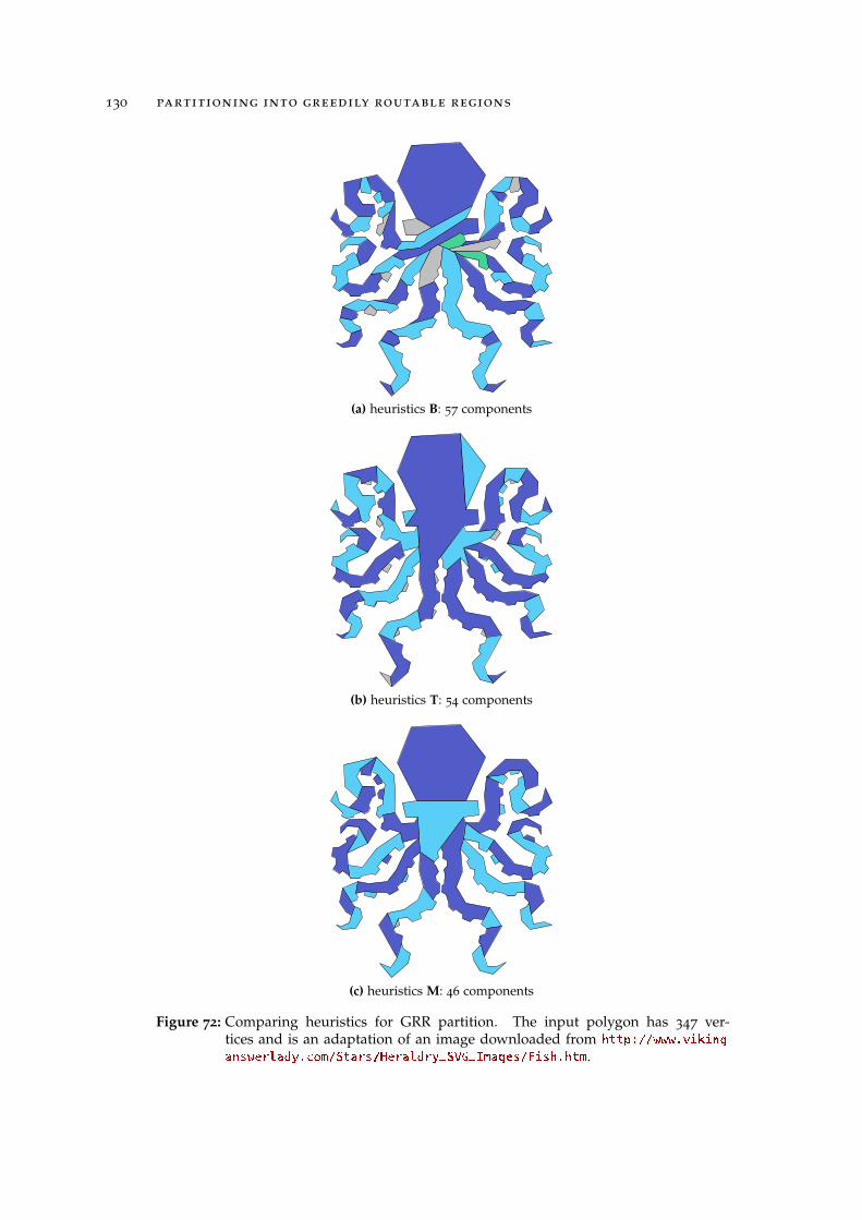
130 partitioning into greedily routable regions

(a) heuristics B: 57 components

(b) heuristics T: 54 components

(c) heuristics M: 46 components

Figure 72: Comparing heuristics for GRR partition. The input polygon has 347 ver-tices and is an adaptation of an image downloaded from http://www.viking

.

answerlady.com/Stars/Heraldry_SVG_Images/Fish.htm

.

.

6.7 conclusion 131

(a) B: 7, T: 7, M: 5 (b) B: 5, T: 4, M: 4

(c) B: 10, T: 13, M: 8 (d) B: 17, T: 18, M: 14

(e) B: 37, T: 33, M: 26 (f) B: 50, T: 58, M: 46

Figure 73: Comparing GRR partition sizes for heuristics B, T and M on six additionalinstances. The figures show the results of heuristics M. The input polygonsare adaptations of images downloaded from http://www.vikinganswerlady.com/Stars/Heraldry_SVG_Images/index.htm

.

.

7C O N C L U S I O N

In this thesis, I have studied the following questions related to greedy routing ongeometrically embedded graphs. 1) Which graphs admit a greedy, self-approach-ing or increasing-chord embedding? 2) What is the complexity of partitioningplane graph drawings and polygons into a small number of components thatsupport greedy routing?

Results from Chapters 4

.

and 5

.

advance the state of knowledge regarding thefirst question. In Chapter 4

.

, I have given the first characterization of trees thatadmit a greedy embedding. Previous research on the existence of greedy embed-dings mainly focused on 3-connected planar graphs and binary cactus graphs.Characterizing greedy-drawable trees is an important next step for tackling theremaining graph classes.

For self-approaching and increasing-chord drawings, the characterization oftrees admitting such drawings has been the only result so far. In Chapter 5

.

, I havecontinued this line of research for other popular and important graph classes. Forexample, I have shown existence of increasing-chord drawings for triangulationsas well as non-existence of self-approaching drawings for families of binary cactusgraphs.

Self-approaching and increasing-chord graph drawings have become a popularresearch topic in the graph drawing and computational geometry community,which lets one hope that new existence results for the remaining graph classeswill follow in the near future.

In Chapter 6

.

, I have extensively studied the complexity of partitioning planegraph drawings into a minimum number of Greedily Routable Regions and haveshown NP-hardness even for partitioning drawings of trees, whereas natural re-strictions thereof turned out to be optimally solvable in polynomial time. Forpartitioning polygons, no such optimal solutions or even polynomial-time approx-imations have been known. The insights gained from studying the GRR partition-ing problem for graph drawings have allowed me to formulate a polynomial-time2-approximation for partitioning hole-free polygons with respect to a given trian-gulation.

133

134 conclusion

consequences for practice

For greedy drawings, negative existence results [PR05

.

; LM10

.

] as well as worst-case exponential area bounds [ADF12

.

] have been known for trees, which leadsone to believe that the vision of using Euclidean greedy embeddings for point-to-point routing is unrealistic for the case when the communication graph is weaklyconnected. The negative existence results for trees as well as worst-case expo-nential area bounds for binary cactuses acquired in this thesis support this belief.Some possibilities to overcome these issues are 1) efficient distributed embeddingtechniques that do not provide a 100% delivery guarantee of the standard greedyrouting [Rao+03

.

; Sar+09

.

], 2) network decomposition techniques similar to the onedescribed in Chapter 6

.

or 3) non-Euclidean greedy embeddings [Kle07

.

].Similarly, for self-approaching and increasing-chord graph drawings, the nega-

tive existence result as well as the worst-case exponential area bound for binarycactuses shown in Chapter 5

.

of this thesis supports the belief that these draw-ing styles are not suited for creating practical drawings of big weakly connectedgraphs. Instead, one could consider using graph drawing styles with weaker no-tions of geodesic-path tendency that are less restrictive, such as monotone draw-ings [Ang+12

.

], and study the possibilities to further improve the practicality andaesthetics of such drawings.

outlook

For each of the considered problems, several remaining open questions are listedat the end of the corresponding chapter. The strong Papadimitriou and Ratajczakconjecture that 3-connected planar graphs have planar convex graph drawings isparticularly worth mentioning here in the light of the recent proof by Da Lozzoet al. [DDF17

.

] that such graphs have planar greedy drawings.In the context of greedy embeddings, an interesting research direction is to

consider algorithmic problems that model aspects of wireless sensor networksthat are important for the practical applicability for routing. Such aspects thathave been considered are, for example, succinctness [EG11

.

; GS09

.

] and efficientdistributed computation [Sar+09

.

; Ben+11

.

] of virtual coordinates, bounded hopstretch [FPW09

.

] and load balancing [Sar+10

.

]. However, combining these aspectswhile maintaining provable guarantees appears challenging. Another challengein this context is node mobility and edge removal due to battery depletions. Thefollowing problem posed by Kleinberg [Kle07

.

] remains open: design a distributedgreedy embedding algorithm that allows reconstructing the greedy embeddingupon node or edge deletion in O(polylog n) amortized time or prove that o(n)amortized time is unachievable.

To use greedy, strongly monotone, self-approaching and increasing-chord draw-ings as a tool to help users find paths in graphs, the drawings should satisfy cer-tain aesthetic criteria such as a low number of crossings and a good resolution.It has been known that greedy drawings of trees require exponential resolution

conclusion 135

in the worst case [ADF12

.

], and I have shown this for strongly monotone treedrawings in Chapter 5

.

. For higher connectivity, e.g., 3-connected graphs, it is stillopen whether there exist graphs that require exponential area for any greedy, self-approaching or increasing-chord drawing. For greedy drawings, this open prob-lem has been stated by Angelini et al. [ADF12

.

]. What about the area requirementsfor planar greedy, self-approaching or increasing-chord drawings of 3-connectedplanar graphs? Another possible research direction is considering combinationswith well-established graph drawing conventions such as orthogonal graph draw-ings. In a joint work with Angelini et al. [Ang+18

.

], we have recently initiated thestudy of greedy rectilinear orthogonal drawings.

We have seen that minimum GRR partition is computationally hard even forvery restricted variants of the problem. For partitioning simple polygons andpolygonal regions into a minimum number of GRRs, a possible direction of futurework is designing and comparing new efficient heuristics. Of particular interestare algorithms that can be efficiently implemented in a distributed setting.

Part III

A P P E N D I X

AA P P E N D I X

Appendix A

.

contains the proof of a sufficient condition for 180, ϕ1, . . . , ϕ4 ∈P5 deferred from Chapter 4

.

.

Lemma 4.25

.

. Consider angles 0 ≤ ϕ4 ≤ 60, 90 < ϕ3 ≤ ϕ2 ≤ ϕ1 ≤ 120, ϕ1 +

. . . + ϕ4 > 360. Let the following two conditions hold:

(i) 14ϕ1 + 12ϕ2 + 8ϕ3 + 15ϕ4 > 4500

(ii) For x := min 17 (14ϕ1 + 12ϕ2 + 8ϕ3 + 15ϕ4 − 4500), ϕ4 and p1 ∈ [0, 90]10,

p1 = (β0, . . . , β4, γ0, . . . , γ4) defined as:

β0 = ϕ4 − x,

β1 = 90 − x2

,

β2 = ϕ3 +ϕ2

2+

ϕ1

4+

ϕ4 − x8− 157.5,

β3 = ϕ2 +ϕ1

2+

ϕ4 − x4− 135,

β4 = ϕ1 − 90 +ϕ4 − x

2,

γ0 = 90 − ϕ4 − x2

,

γ1 = x,

γ2 = 168.75 − ϕ3

2− ϕ2

4− ϕ1

8− ϕ4 − x

16,

γ3 = 157.5 − ϕ2

2− ϕ1

4− ϕ4 − x

8,

γ4 = 135 − ϕ1

2− ϕ4 − x

4,

it holds: ω(p1) < 0.

Then, 180, ϕ1, . . . , ϕ4 ∈ P5.

Proof. Assume both conditions hold. See the construction in Figure 74

.

. The anglesin p1 are chosen such that all five triangles are equilateral: we have β1 = α1

139

140 appendix

β0

γ0

γ1β1

γ4

β2

β3

β4

γ3γ2

ψ4

ψ1

ψ2

ψ3

≤ 180

= x

Figure 74: Proof of Lemma 4.25

.

.

and γi = αi for i = 0, 2, 3, 4. Furthermore, β0, γ1, β2, β3, β4 ≤ 60. Consider thepermutation τ = (4, 0, 3, 2, 1). We verify the conditions in Observation 4.3

.

:

β4 + γ0 = ϕ1

β3 + γ4 = ϕ2

β2 + γ3 = ϕ3

β1 + γ2 = 258.75 − 18

ϕ1 −14

ϕ2 −12

ϕ3 −1

16ϕ4 −

716

x ≤ 180

β0 + γ1 = ϕ4

2β0 + γ0 =32

ϕ4 −32

x + 90 ≤ 180

2β1 + γ1 = 180

2β2 + γ2 =38

ϕ1 +34

ϕ2 +32

ϕ3 +3

16ϕ4 −

316

x− 146.25 ≤ 180

2β3 + γ3 =34

ϕ1 +32

ϕ2 +38

ϕ4 −38

x− 112.5 ≤ 180

2β4 + γ4 =32

ϕ1 +34

ϕ4 −34

x− 45 ≤ 180

β0 + 2γ0 = 180

β1 + 2γ1 = 90 +32

x ≤ 180

β2 + 2γ2 = 180

β3 + 2γ3 = 180

β4 + 2γ4 = 180

We see that p1 lies in the polytope Pτ =: P, in particular, p1 ∈ ∂P.We now define another point p2 ∈ [0, 90]10. Due to condition (i), there must

exist 90 < ψi < ϕi for i = 1, . . . , 3, 0 < ψ4 < ϕ4, 0 < ε < ψ4 (for proper ψi, ε

can be chosen arbitrarily small), such that:

14ψ1 + 12ψ2 + 8ψ3 + 15ψ4 − 80ε = 4500.

appendix 141

Consider the point p2 = (β0, . . . , β4, γ0, . . . , γ4), such that:

β0 = ψ4,

β1 = 90 − ε,

β2 = ψ3 +ψ2

2+

ψ1

4+

ψ4

8− 157.5,

β3 = ψ2 +ψ1

2+

ψ4

4− 135,

β4 = ψ1 − 90 +ψ4

2,

γ0 = 90 − ψ4

2− ε,

γ1 = 0,

γ2 = 168.75 − ψ3

2− ψ2

4− ψ1

8− ψ4

16− ε,

γ3 = 157.5 − ψ2

2− ψ1

4− ψ4

8− ε,

γ4 = 135 − ψ1

2− ψ4

4− ε.

The condition ∑4i=0(βi + γi) = 540 holds, since

164

∑i=0

(βi + γi) = 16 · (90 + 168.75) + (14ψ1 + 12ψ2 + 8ψ3 + 15ψ4 − 16 · 5ε)

= 16 · 540

due to the choice of ψi and ε. The rest of the conditions for p2 ∈ P can be easilyverified:

β4 + γ0 = ψ1 − ε < ϕ1

β3 + γ4 = ψ2 − ε < ϕ2

β2 + γ3 = ψ3 − ε < ϕ3

β1 + γ2 = 258.75 − 18

ψ1 −14

ψ2 −12

ψ3 −116

ψ4 − 2ε < 180

β0 + γ1 = ψ4 < ϕ4

2β0 + γ0 =32

ψ4 + 90 − ε < 180

2β1 + γ1 = 180 − 2ε < 180

2β2 + γ2 =38

ψ1 +34

ψ2 +32

ψ3 +316

ψ4 − ε− 146.25 < 180

2β3 + γ3 =34

ψ1 +32

ψ2 +38

ψ4 − ε− 112.5 < 180

2β4 + γ4 =32

ψ1 +34

ψ4 − ε− 45 < 180

142 appendix

β0 + 2γ0 = 180 − 2ε < 180

β1 + 2γ1 = 90 − ε < 180

β2 + 2γ2 = 180 − 2ε < 180

β3 + 2γ3 = 180 − 2ε < 180

β4 + 2γ4 = 180 − 2ε < 180

Apart from γ1 ≥ 0, all inequalities are strict. Since γ1 > 0, for each λ ∈ (0, 1),the point λp1 + (1− λ)p2 lies in the interior of P. Since ω(p1) < 0 and ω(p2) >

0 (due to γ1 = 0), by the mean value theorem, ω(λp1 + (1 − λ)p2) = 0 forsome λ ∈ (0, 1).

B I B L I O G R A P H Y

[ACM89] Esther M. Arkin, Robert Connelly, and Joseph S. B. Mitchell. „On Mono-tone Paths Among Obstacles with Applications to Planning Assem-blies.“ In: Proc. 5th Ann. ACM Symp. Computational Geometry (SoCG’89).ACM, 1989, 334–343. doi: 10.1145/73833.73870

.

.

[ADF12] Patrizio Angelini, Giuseppe Di Battista, and Fabrizio Frati. „SuccinctGreedy Drawings Do Not Always Exist.“ In: Networks 59.3 (2012), 267–274. doi: 10.1002/net.21449

.

.

[AFG10] Patrizio Angelini, Fabrizio Frati, and Luca Grilli. „An Algorithm to Con-struct Greedy Drawings of Triangulations.“ In: J. Graph Algorithms Appl.14.1 (2010), 19–51. doi: 10.7155/jgaa.00197

.

.

[Aic+01] Oswin Aichholzer, Franz Aurenhammer, Christian Icking, Rolf Klein,Elmar Langetepe, and Günter Rote. „Generalized Self-ApproachingCurves.“ In: Discrete Appl. Math. 109 (1–2 2001), 3–24. doi: 10.1016/S0166-218X(00)00233-X

.

.

[AK04] Jamal N. Al-Karaki and Ahmed E. Kamal. „Routing Techniques in Wire-less Sensor Networks: A Survey.“ In: IEEE Wireless Communications 11.6(2004), 6–28. doi: 10.1109/MWC.2004.1368893

.

.

[Ala+13] Soroush Alamdari, Timothy M. Chan, Elyot Grant, Anna Lubiw, andVinayak Pathak. „Self-Approaching Graphs.“ In: Proc. 20th Internat.Symp. Graph Drawing (GD’12). Ed. by Walter Didimo and Maurizio Pa-trignani. Vol. 7704 of Lecture Notes Comput. Sci. Springer, 2013, 260–271.doi: 10.1007/978-3-642-36763-2_23

.

.

[AM12] Eiman Alotaibi and Biswanath Mukherjee. „A Survey on Routing Algo-rithms for Wireless Ad-Hoc and Mesh Networks.“ In: Computer Networks56.2 (2012), 940–965. doi: 10.1016/j.comnet.2011.10.011

.

.

[Ang+12] Patrizio Angelini, Enrico Colasante, Giuseppe Di Battista, Fabrizio Frati,and Maurizio Patrignani. „Monotone Drawings of Graphs.“ In: J. GraphAlgorithms Appl. 16.1 (2012), 5–35. doi: 10.7155/jgaa.00249

.

.

[Ang+15] Patrizio Angelini, Walter Didimo, Stephen G. Kobourov, Tamara Mched-lidze, Vincenzo Roselli, Antonios Symvonis, and Stephen Wismath.„Monotone Drawings of Graphs with Fixed Embedding.“ In: Algorith-mica 71.2 (2015), 233–257. doi: 10.1007/s00453-013-9790-3

.

.

[Ang+18] Patrizio Angelini, Michael A. Bekos, Walter Didimo, Luca Grilli, Phil-ipp Kindermann, Tamara Mchedlidze, Roman Prutkin, Antonios Sym-vonis, and Alessandra Tappini. „Greedy Rectilinear Orthogonal Draw-ings.“ Under submission. 2018.

143

144 bibliography

[Ang17] Patrizio Angelini. „Monotone Drawings of Graphs with Few Direc-tions.“ In: Information Processing Letters 120 (2017), 16–22. doi: 10.1016/j.ipl.2016.12.004

.

.

[AV10] Ian F. Akyildiz and Mehmet Can Vuran. Wireless Sensor Networks. JohnWiley & Sons, 2010. doi: 10.1002/9780470515181

.

.

[Bah+17] Yeganeh Bahoo, Stephane Durocher, Sahar Mehrpour, and DebajyotiMondal. „Exploring Increasing-Chord Paths and Trees.“ In: Proc. 29thCanadian Conf. Computational Geometry (CCCG’17). 2017, 19–24. arXiv:1702.08380

.

.

[Bar66] David Barnette. „Trees in Polyhedral Graphs.“ In: Canadian J. Math. 18(1966), 731–736. doi: 10.4153/CJM-1966-073-4

.

.

[Ben+11] Mirela Ben Chen, Steven J. Gortler, Craig Gotsman, and CamilleWormser. „Distributed Computation of Virtual Coordinates for GreedyRouting in Sensor Networks.“ In: Discrete Appl. Math. 159.7 (2011), 544–560. doi: 10.1016/j.dam.2010.10.016

.

.

[BGJ07] Jehoshua Bruck, Jie Gao, and Anxiao (Andrew) Jiang. „MAP: MedialAxis Based Geometric Routing in Sensor Networks.“ In: Wireless Net-works 13.6 (2007), 835–853. doi: 10.1007/s11276-006-9857-z

.

.

[Bir+11] Michael Biro, Jie Gao, Justin Iwerks, Irina Kostitsyna, and Joseph S. B.Mitchell. „Beacon-Based Routing and Coverage.“ In: Proc. 21st Fall Work-shop on Computational Geometry (FWCG’11). 2011.

[Bir+13] Michael Biro, Justin Iwerks, Irina Kostitsyna, and Joseph S. B. Mitchell.„Beacon-Based Algorithms for Geometric Routing.“ In: Proc. 13th In-ternat. Symp. Algorithms and Data Structures (WADS’13). Ed. by FrankDehne, Roberto Solis-Oba, and Jörg-Rüdiger Sack. Vol. 8037 of LectureNotes Comput. Sci. Springer, 2013, 158–169. doi: 10.1007/978-3-642-40104-6_14

.

.

[Bir13] Michael Biro. „Beacon-Based Routing and Guarding.“ PhD thesis. StateUniversity of New York at Stony Brook, Department of Applied Mathe-matics and Statistics, 2013.

[BKL17] Prosenjit Bose, Irina Kostitsyna, and Stefan Langerman. „Self-approaching paths in simple polygons.“ In: Proc. 33rd Internat. Symp.Computational Geometry (SoCG’17). Ed. by Boris Aronov and MatthewJ. Katz. Vol. 77 of Leibniz International Proceedings in Informatics (LIPIcs).Schloss Dagstuhl–Leibniz-Zentrum für Informatik, 2017, 21:1–21:15. doi:10.4230/LIPIcs.SoCG.2017.21

.

.

[BM04] Prosenjit Bose and Pat Morin. „Online Routing in Triangulations.“ In:SIAM J. Comput. 33.4 (2004), 937–951. doi: 10.1137/S0097539700369387

.

.

bibliography 145

[Bon+16] Nicolas Bonichon, Prosenjit Bose, Paz Carmi, Irina Kostitsyna, AnnaLubiw, and Sander Verdonschot. „Gabriel Triangulations and Angle-Monotone Graphs: Local Routing and Recognition.“ In: Proc. 24th In-ternat. Symp. Graph Drawing and Network Visualization (GD’16). Ed. byYifan Hu and Martin Nöllenburg. Vol. 9801 of Lecture Notes Comput. Sci.Springer, 2016, 519–531. doi: 10.1007/978-3-319-50106-2_40

.

.

[Bon+17] Nicolas Bonichon, Prosenjit Bose, Jean-Lou Carufel, Ljubomir Perkovic,and André van Renssen. „Upper and Lower Bounds for Online Routingon Delaunay Triangulations.“ In: Discrete Comput. Geom. 58.2 (2017), 482–504. doi: 10.1007/s00454-016-9842-y

.

.

[Bos+01] Prosenjit Bose, Pat Morin, Ivan Stojmenovic, and Jorge Urrutia. „Routingwith Guaranteed Delivery in Ad Hoc Wireless Networks.“ In: WirelessNetworks 7.6 (2001), 609–616. doi: 10.1023/A:1012319418150

.

.

[Bos+02] Prosenjit Bose, Andrej Brodnik, Svante Carlsson, Erik D. Demaine,Rudolf Fleischer, Alejandro López-Ortiz, Pat Morin, and J. Ian Munro.„Online Routing in Convex Subdivisions.“ In: Internat. J. Comput. Geom.Appl. 12.4 (2002), 283–295. doi: 10.1142/S021819590200089X

.

.

[Bos+12] Prosenjit Bose, Rolf Fagerberg, André van Renssen, and Sander Verdon-schot. „Competitive Routing in the Half-Θ6-Graph.“ In: Proc. 23rd ACM-SIAM Symp. Discrete Algorithms (SODA’12). SIAM, 2012, 1319–1328. doi:10.1137/1.9781611973099.104

.

.

[Bos+15] Prosenjit Bose, Stephane Durocher, Debajyoti Mondal, Maxime Peabody,Matthew Skala, and Mohammad Abdul Wahid. „Local Routing in Con-vex Subdivisions.“ In: Proc. 41st Internat. Conf. Current Trends in Theoryand Practice of Computer Science (SOFSEM’15). Ed. by Giuseppe F. Italiano,Tiziana Margaria-Steffen, Jaroslav Pokorný, Jean-Jacques Quisquater,and Roger Wattenhofer. Vol. 8939 of Lecture Notes Comput. Sci. Springer,2015, 140–151. doi: 10.1007/978-3-662-46078-8_12

.

.

[Bou+08] Azzedine Boukerche, Mohammad Z. Ahmad, Damla Turgut, and Be-gumhan Turgut. „A Taxonomy of Routing Protocols in Sensor Net-works.“ In: Algorithms and Protocols for Wireless Sensor Networks. Ed. byAzzedine Boukerche. John Wiley & Sons, 2008, 129–160. doi: 10.1002/9780470396360.ch6

.

.

[Bou08] Azzedine Boukerche, ed. Algorithms and Protocols for Wireless Sensor Net-works. John Wiley & Sons, 2008. doi: 10.1002/9780470396360

.

.

[BS13] Prosenjit Bose and Michiel Smid. „On Plane Geometric Spanners: A Sur-vey and Open Problems.“ In: Comput. Geom. Theory Appl. 46.7 (2013),818–830. doi: 10.1016/j.comgeo.2013.04.002

.

.

[CA06] Qing Cao and Tarek Abdelzaher. „Scalable Logical Coordinates Frame-work for Routing in Wireless Sensor Networks.“ In: ACM Trans. SensorNetworks 2.4 (2006), 557–593. doi: 10.1145/1218556.1218561

.

.

146 bibliography

[Car+05] Antonio Caruso, Stefano Chessa, Swades De, and Alessandro Urpi.„GPS Free Coordinate Assignment and Routing in Wireless Sensor Net-works.“ In: Proc. 24th IEEE Internat. Conf. Computer Communications (IN-FOCOM’05). IEEE, 2005, 150–160. doi: 10.1109/INFCOM.2005.1497887

.

.

[CD85] Bernard Chazelle and David P. Dobkin. „Optimal Convex Decomposi-tions.“ In: Computational Geometry. Ed. by Godfried T. Toussaint. Vol. 2of Machine Intelligence and Pattern Recognition. North-Holland, 1985, 63–133. doi: 10.1016/B978-0-444-87806-9.50009-8

.

.

[CFR03] Gruia Calinescu, Cristina G. Fernandes, and Bruce Reed. „Multicuts inUnweighted Graphs and Digraphs with Bounded Degree and BoundedTree-Width.“ In: J. Algorithms 48.2 (2003), 333–359. doi: 10.1016/S0196-6774(03)00073-7

.

.

[Cha15] Nessrine Chakchouk. „A Survey on Opportunistic Routing in WirelessCommunication Networks.“ In: IEEE Communications Surveys and Tutori-als 17.4 (2015), 2214–2241. doi: 10.1109/COMST.2015.2411335

.

.

[Che14] Shiri Chechik. „Compact Routing Schemes.“ In: Encyclopedia of Algo-rithms. Ed. by Ming-Yang Kao. Springer, 2014, 1–3. doi: 10.1007/978-3-642-27848-8_561-1

.

.

[Che89] L. Paul Chew. „There Are Planar Graphs Almost as Good as the Com-plete Graph.“ In: J. Computer and System Sciences 39.2 (1989), 205–219. doi:10.1016/0022-0000(89)90044-5

.

.

[CKW15] Ante Custic, Bettina Klinz, and Gerhard J. Woeginger. „Geometric Ver-sions of the Three-Dimensional Assignment Problem under GeneralNorms.“ In: Discrete Optimization 18 (2015), 38–55. doi: 10 . 1016 / j .

disopt.2015.07.002

.

.

[CL03] Bennett Chow and Feng Luo. „Combinatorial Ricci Flows on Sur-faces.“ In: J. Differential Geom. 63.1 (2003), 97–129. doi: 10.4310/jdg/1080835659

.

.

[CLR03] Marie-Christine Costa, Lucas Létocart, and Frédéric Roupin. „A GreedyAlgorithm for Multicut and Integral Multiflow in Rooted Trees.“ In: Op-erations Research Letters 31.1 (2003), 21–27. doi: 10.1016/S0167-6377(02)00184-0

.

.

[CLR05] Marie-Christine Costa, Lucas Létocart, and Frédéric Roupin. „MinimalMulticut and Maximal Integer Multiflow: A Survey.“ In: European J. Op-erational Research 162.1 (2005), 55–69. doi: 10.1016/j.ejor.2003.10.037

.

.

[Com00] Douglas E. Comer. Internetworking with TCP/IP, Volume 1: Principles, Pro-tocols, and Architectures. 4th edition. Prentice Hall, 2000.

bibliography 147

[DDF17] Giordano Da Lozzo, Anthony D’Angelo, and Fabrizio Frati. „On pla-nar greedy drawings of 3-connected planar graphs.“ In: Proc. 33rd Inter-nat. Symp. Computational Geometry (SoCG’17). Ed. by Boris Aronov andMatthew J. Katz. Vol. 77 of Leibniz International Proceedings in Informatics(LIPIcs). Schloss Dagstuhl–Leibniz-Zentrum für Informatik, 2017, 33:1–33:16. doi: 10.4230/LIPIcs.SoCG.2017.33

.

.

[DFG15] Hooman Reisi Dehkordi, Fabrizio Frati, and Joachim Gudmundsson.„Increasing-Chord Graphs on Point Sets.“ In: J. Graph Algorithms Appl.19.2 (2015), 761–778. doi: 10.7155/jgaa.00348

.

.

[DFS90] David P. Dobkin, Steven J. Friedman, and Kenneth J. Supowit. „DelaunayGraphs Are Almost as Good as Complete Graphs.“ In: Discrete Comput.Geom. 5.4 (1990), 399–407. doi: 10.1007/BF02187801

.

.

[DGW15] Stephane Durocher, Leszek Gasieniec, and Prudence W.H. Wong. „Rout-ing in Geometric Networks.“ In: Encyclopedia of Algorithms. Ed. by Ming-Yang Kao. Springer, 2015, 1–5. doi: 10.1007/978-3-642-27848-8_352-2

.

.

[Dha10] Raghavan Dhandapani. „Greedy Drawings of Triangulations.“ In: Dis-crete Comput. Geom. 43.2 (2010), 375–392. doi: 10.1007/s00454- 009-9235-6

.

.

[DKN10] Stephane Durocher, David Kirkpatrick, and Lata Narayanan. „On Rout-ing with Guaranteed Delivery in Three-Dimensional Ad Hoc WirelessNetworks.“ In: Wireless Networks 16.1 (2010), 227–235. doi: 10 . 1007 /

s11276-008-0126-1

.

.

[DKR15] Søren Dahlgaard, Mathias Bæk Tejs Knudsen, and Noy Rotbart. „A Sim-ple and Optimal Ancestry Labeling Scheme for Trees.“ In: Proc. 42nd In-ternat. Colloquium on Automata, Languages, and Programming (ICALP’15).Ed. by Magnús M. Halldórsson, Kazuo Iwama, Naoki Kobayashi, andBettina Speckmann. Vol. 9135 of Lecture Notes Comput. Sci. Springer, 2015,564–574. doi: 10.1007/978-3-662-47666-6_45

.

.

[DS05] David M. Doolin and Nicholas Sitar. „Wireless Sensors for Wildfire Mon-itoring.“ In: Proc. SPIE 12th Int. Symp. Smart Structures and Materials. Vol.5765 of SPIE. 2005, 477–484. doi: 10.1117/12.605655

.

.

[DV96] Giuseppe Di Battista and Luca Vismara. „Angles of Planar TriangularGraphs.“ In: SIAM J. Discrete Math. 9.3 (1996), 349–359. doi: 10.1137/S0895480194264010

.

.

[EG11] David Eppstein and Michael T. Goodrich. „Succinct Greedy GeometricRouting Using Hyperbolic Geometry.“ In: IEEE Trans. Computers 60.11(2011), 1571–1580. doi: 10.1109/TC.2010.257

.

.

[Epp00] David Eppstein. „Spanning Trees and Spanners.“ In: Handbook of Com-putational Geometry. Ed. by Jörg-Rüdiger Sack and Jorge Urrutia. North-Holland, 2000, 425–461. doi: 10.1016/B978-044482537-7/50010-3

.

.

148 bibliography

[Fan+05] Qing Fang, Jie Gao, Leonidas J. Guibas, Vin de Silva, and Li Zhang.„GLIDER: Gradient Landmark-Based Distributed Routing for SensorNetworks.“ In: Proc. 24th IEEE Internat. Conf. Computer Communications(INFOCOM’05). Vol. 1. IEEE, 2005, 339–350. doi: 10.1109/INFCOM.2005.1497904

.

.

[Fel+16] Stefan Felsner, Alexander Igamberdiev, Philipp Kindermann, BorisKlemz, Tamara Mchedlidze, and Manfred Scheucher. „Strongly Mono-tone Drawings of Planar Graphs.“ In: Proc. 32nd Internat. Symp. Com-putational Geometry (SoCG’16). Ed. by Sándor Fekete and Anna Lubiw.Vol. 51 of Leibniz International Proceedings in Informatics (LIPIcs). SchlossDagstuhl–Leibniz-Zentrum für Informatik, 2016, 37:1–37:15. doi: 10 .

4230/LIPIcs.SoCG.2016.37

.

.

[Fel04] Stefan Felsner. „Schnyder Woods or How to Draw a Planar Graph?“In: Geometric Graphs and Arrangements. Advanced Lectures in Mathematics.Vieweg Verlag, 2004, 17–42. doi: 10.1007/978-3-322-80303-0_2

.

.

[Fin87] Gregory G. Finn. Routing and Addressing Problems in Large Metropolitan-Scale Internetworks. Technical report ISI/RR-87-180. University of South-ern California, Marina del Rey, Information Sciences Institute, 1987.

[FM07] Stefan Funke and Nikola Milosavljevic. „Guaranteed-Delivery Geo-graphic Routing Under Uncertain Node Locations.“ In: Proc. 26th IEEEInternat. Conf. Computer Communications (INFOCOM’07). IEEE, 2007,1244–1252. doi: 10.1109/INFCOM.2007.148

.

.

[Fon+05] Rodrigo Fonseca, Sylvia Ratnasamy, Jerry Zhao, Cheng Tien Ee,David Culler, Scott Shenker, and Ion Stoica. „Beacon Vector Rout-ing: Scalable Point-to-Point Routing in Wireless Sensornets.“ In: Proc.2nd Usenix/ACM Symp. Networked Systems Design and Implementation(NSDI’05). USENIX Association, 2005, 329–342.

[FPW09] Roland Flury, Sriram V. Pemmaraju, and Roger Wattenhofer. „GreedyRouting with Bounded Stretch.“ In: Proc. 28th IEEE Internat. Conf. Com-puter Communications (INFOCOM’09). IEEE, 2009, 1737–1745. doi: 10 .

1109/INFCOM.2009.5062093

.

.

[FRS09] Hannes Frey, Stefan Rührup, and Ivan Stojmenovic. „Routing in Wire-less Sensor Networks.“ In: Guide to Wireless Sensor Networks. Ed. by Sub-has Chandra Misra, Isaac Woungang, and Sudip Misra. Computer Com-munications and Networks. Springer, 2009, 81–111. doi: 10.1007/978-1-84882-218-4_4

.

.

[FS06] Hannes Frey and Ivan Stojmenovic. „On Delivery Guarantees of Faceand Combined Greedy-Face Routing in Ad Hoc and Sensor Networks.“In: Proc. 12th ACM Internat. Conf. Mobile Computing and Networking (Mo-biCom’06). ACM, 2006, 390–401. doi: 10.1145/1161089.1161133

.

.

bibliography 149

[Gao+05] Jie Gao, Leonidas J. Guibas, John Hershberger, Li Zhang, and An Zhu.„Geometric Spanners for Routing in Mobile Networks.“ In: IEEE J. Se-lected Areas in Communications 23.1 (2005), 174–185. doi: 10.1109/JSAC.2004.837364

.

.

[GG12] Jie Gao and Leonidas J. Guibas. „Geometric Algorithms for Sensor Net-works.“ In: Phil. Trans. R. Soc. A 370.1958 (2012), 27–51. doi: 10.1098/rsta.2011.0215

.

.

[GGL15] Jie Gao, Xianfeng David Gu, and Feng Luo. „Discrete Ricci Flow forGeometric Routing.“ In: Encyclopedia of Algorithms. Ed. by Ming-YangKao. Springer, 2015, 1–8. doi: 10.1007/978-3-642-27848-8_602-1

.

.

[GS09] Michael T. Goodrich and Darren Strash. „Succinct Greedy GeometricRouting in the Euclidean Plane.“ In: Proc. 20th Internat. Symp. Algorithmsand Computation (ISAAC’09). Ed. by Yingfei Dong, Ding-Zhu Du, andOscar Ibarra. Vol. 5878 of Lecture Notes Comput. Sci. Springer, 2009, 781–791. doi: 10.1007/978-3-642-10631-6_79

.

.

[GUR7.5] Gurobi Optimizer. Version 7.5. Gurobi Optimization, Inc. 2017. url: http://www.gurobi.com

.

.

[GVY97] Naveen Garg, Vijay V. Vazirani, and Mihalis Yannakakis. „Primal-DualApproximation Algorithms for Integral Flow and Multicut in Trees.“ In:Algorithmica 18.1 (1997), 3–20. doi: 10.1007/BF02523685

.

.

[HE05] Weidong Huang and Peter Eades. „How People Read Graphs.“ In: Proc.4th Asia Pacific Symposium on Information Visualisation (APVIS’05). Aus-tralian Comput. Soc., 2005, 51–58.

[HEH09] Weidong Huang, Peter Eades, and Seok-Hee Hong. „A Graph ReadingBehavior: Geodesic-Path Tendency.“ In: Proc. 2nd IEEE Pacific Visualiza-tion Symp. (PacificVis’09). IEEE, 2009, 137–144. doi: 10.1109/PACIFICVIS.2009.4906848

.

.

[HH15] Xin He and Dayu He. „Monotone Drawings of 3-Connected PlaneGraphs.“ In: Proc. 23rd European Symp. Algorithms (ESA’15). Ed. byNikhil Bansal and Irene Finocchi. Vol. 9294 of Lecture Notes Comput. Sci.Springer, 2015, 729–741. doi: 10.1007/978-3-662-48350-3_61

.

.

[HH17] Dayu He and Xin He. „Optimal Monotone Drawings of Trees.“ In: SIAMJ. Discrete Math. (2017), 1867–1877. doi: 10.1137/16M1080045

.

.

[HR15] Md. Iqbal Hossain and Md. Saidur Rahman. „Good Spanning Trees inGraph Drawing.“ In: Theoret. Comput. Sci. 607.2 (2015), 149–165. doi: 10.1016/j.tcs.2015.09.004

.

.

[Hua07] Weidong Huang. „Using Eye Tracking to Investigate Graph Layout Ef-fects.“ In: Proc. 6th Internat. Asia-Pacific Symp. Visualization (APVIS’07).IEEE, 2007, 97–100. doi: 10.1109/APVIS.2007.329282

.

.

150 bibliography

[IKL99] Christian Icking, Rolf Klein, and Elmar Langetepe. „Self-ApproachingCurves.“ In: Math. Proc. Camb. Phil. Soc. 125.3 (1999), 441–453. doi: 10.1017/S0305004198003016

.

.

[Jia+15] Hongbo Jiang, Tianlong Yu, Chen Tian, Guang Tan, and ChonggangWang. „Connectivity-Based Segmentation in Large-Scale 2-D/3-D Sen-sor Networks: Algorithm and Applications.“ In: IEEE/ACM Trans. Net-working 23.1 (2015), 15–27. doi: 10.1109/TNET.2013.2289912

.

.

[JM96] David B. Johnson and David A. Maltz. „Dynamic Source Routing in AdHoc Wireless Networks.“ In: Mobile Computing. Ed. by Tomasz Imielin-ski and Henry F. Korth. Vol. 353 of The Kluwer International Series in En-gineering and Computer Science. Kluwer Academic Publishers, 1996, 153–181. doi: 10.1007/978-0-585-29603-6_5

.

.

[Kei00] J. Mark Keil. „Polygon Decomposition.“ In: Handbook of ComputationalGeometry. Ed. by Jörg-Rüdiger Sack and Jorge Urrutia. North-Holland,2000, 491–518. doi: 10.1016/B978-044482537-7/50012-7

.

.

[Kei85] J. Mark Keil. „Decomposing a Polygon into Simpler Components.“ In:SIAM J. Comput. 14.4 (1985), 799–817. doi: 10.1137/0214056

.

.

[Kim+05a] Young-Jin Kim, Ramesh Govindan, Brad Karp, and Scott Shenker. „Ge-ographic Routing Made Practical.“ In: Proc. 2nd Usenix/ACM Symp. Net-worked Systems Design and Implementation (NSDI’05). USENIX Associa-tion, 2005, 217–230.

[Kim+05b] Young-Jin Kim, Ramesh Govindan, Brad Karp, and Scott Shenker. „Onthe Pitfalls of Geographic Face Routing.“ In: Proc. Joint Workshop on Foun-dations of Mobile Computing (DIALM-POMC’05). ACM, 2005, 34–43. doi:10.1145/1080810.1080818

.

.

[Kin+14] Philipp Kindermann, André Schulz, Joachim Spoerhase, and AlexanderWolff. „On Monotone Drawings of Trees.“ In: Proc. 22nd Internat. Symp.Graph Drawing (GD’14). Ed. by Christian A. Duncan and Antonios Sym-vonis. Vol. 8871 of Lecture Notes Comput. Sci. Springer, 2014, 488–500. doi:10.1007/978-3-662-45803-7_41

.

.

[KK00] Brad Karp and H. T. Kung. „GPSR: Greedy Perimeter Stateless Routingfor Wireless Networks.“ In: Proc. 6th ACM Internat. Conf. Mobile Comput-ing and Networking (MobiCom’00). ACM, 2000, 243–254. doi: 10.1145/345910.345953

.

.

[Kle07] Robert Kleinberg. „Geographic Routing Using Hyperbolic Space.“ In:Proc. 26th IEEE Internat. Conf. Computer Communications (INFOCOM’07).IEEE, 2007, 1902–1909. doi: 10.1109/INFCOM.2007.221

.

.

[KNR92] Sampath Kannan, Moni Naor, and Steven Rudich. „Implicit Represen-tation of Graphs.“ In: SIAM J. Discrete Math. 5.4 (1992), 596–603. doi:10.1137/0405049

.

.

bibliography 151

[Kob12] Stephen G. Kobourov. Spring Embedders and Force Directed Graph DrawingAlgorithms. 2012. arXiv: 1201.3011

.

.

[KR92] Donald E. Knuth and Arvind Raghunathan. „The Problem of Compati-ble Representatives.“ In: SIAM J. Discrete Math. 5.3 (1992), 422–427. doi:10.1137/0405033

.

.

[KSU99] Evangelos Kranakis, Harvinder Singh, and Jorge Urrutia. „CompassRouting on Geometric Networks.“ In: Proc. 11th Canadian Conf. Computa-tional Geometry (CCCG’99). 1999, 51–54.

[KW05] Holger Karl and Andreas Willig. Protocols and Architectures for WirelessSensor Networks. John Wiley & Sons, 2005. doi: 10.1002/0470095121

.

.

[KWZ08a] Fabian Kuhn, Roger Wattenhofer, and Aaron Zollinger. „Ad Hoc Net-works Beyond Unit Disk Graphs.“ In: Wireless Networks 14.5 (2008), 715–729. doi: 10.1007/s11276-007-0045-6

.

.

[KWZ08b] Fabian Kuhn, Roger Wattenhofer, and Aaron Zollinger. „An AlgorithmicApproach to Geographic Routing in Ad Hoc and Sensor Networks.“ In:IEEE/ACM Trans. Networking 16.1 (2008), 51–62. doi: 10.1109/TNET.2007.900372

.

.

[LA06] Ke Liu and Nael Abu-Ghazaleh. „Aligned Virtual Coordinates forGreedy Routing in WSNs.“ In: Proc. 3rd IEEE Internat. Conf. Mobile Ad-hoc and Sensor Systems (MASS’06). IEEE, 2006, 377–386. doi: 10.1109/MOBHOC.2006.278577

.

.

[Lee+06] Bongshin Lee, Catherine Plaisant, Cynthia Sims Parr, Jean-Daniel Fekete,and Nathalie Henry. „Task Taxonomy for Graph Visualization.“ In: Proc.AVI Workshop on BEyond Time and Errors: Novel Evaluation Methods forInformation Visualization (BELIV’06). ACM, 2006, 1–5. doi: 10 . 1145 /

1168149.1168168

.

.

[Li+00] Jinyang Li, John Jannotti, Douglas S. J. De Couto, David R. Karger, andRobert Morris. „A Scalable Location Service for Geographic Ad HocRouting.“ In: Proc. 6th ACM Internat. Conf. Mobile Computing and Network-ing (MobiCom’00). ACM, 2000, 120–130. doi: 10.1145/345910.345931

.

.

[Li+05] Chih-ping Li, Wei-jen Hsu, Bhaskar Krishnamachari, and Ahmed Helmy.„A Local Metric for Geographic Routing with Power Control in WirelessNetworks.“ In: Proc. 2nd Ann. IEEE Communications Society Conf. Sensorand Ad Hoc Communications and Networks (SECON’05). IEEE, 2005, 229–239. doi: 10.1109/SAHCN.2005.1557078

.

.

[Lic82] David Lichtenstein. „Planar Formulae and Their Uses.“ In: SIAM J. Com-put. 11.2 (1982), 329–343. doi: 10.1137/0211025

.

.

[Lin82] Andrzej Lingas. „The Power of Non-Rectilinear Holes.“ In: Proc. 9th In-ternat. Colloquium on Automata, Languages, and Programming (ICALP’82).Ed. by Erik Meineche Schmidt and Mogens Nielsen. Vol. 140 of LectureNotes Comput. Sci. Springer, 1982, 369–383. doi: 10.1007/BFb0012784

.

.

152 bibliography

[LLM06] Ben Leong, Barbara Liskov, and Robert Morris. „Geographic RoutingWithout Planarization.“ In: Proc. 3rd Usenix/ACM Symp. Networked Sys-tems Design and Implementation (NSDI’06). USENIX Association, 2006,339–352.

[LLM07] Ben Leong, Barbara Liskov, and Robert Morris. „Greedy Virtual Coordi-nates for Geographic Routing.“ In: Proc. 15th IEEE Internat. Conf. NetworkProtocols (ICNP’07). IEEE, 2007, 71–80. doi: 10.1109/ICNP.2007.4375838

.

.

[LLW88] Nati Linial, Laszlo Lovász, and Avi Wigderson. „Rubber Bands, ConvexEmbeddings and Graph Connectivity.“ In: Combinatorica 8.1 (1988), 91–102. doi: 10.1007/BF02122557

.

.

[LM10] Tom Leighton and Ankur Moitra. „Some Results on Greedy Embeddingsin Metric Spaces.“ In: Discrete Comput. Geom. 44.3 (2010), 686–705. doi:10.1007/s00454-009-9227-6

.

.

[LO17] Anna Lubiw and Joseph O’Rourke. „Angle-Monotone Paths in Non-Obtuse Triangulations.“ In: Proc. 29th Canadian Conf. Computational Ge-ometry (CCCG’17). 2017, 25–30. arXiv: 1707.00219

.

.

[ML08] Ankur Moitra and Tom Leighton. „Some Results on Greedy Embed-dings in Metric Spaces.“ Presentation given at the 49th Ann. IEEE Symp.Foundations of Computer Science (FOCS’08). 2008. url: http://people.csail.mit.edu/moitra/docs/ftl.pdf

.

.

[MS15] Konstantinos Mastakas and Antonios Symvonis. „On the Constructionof Increasing-Chord Graphs on Convex Point Sets.“ In: Proc. 6th Inter-nat. Conf. Information, Intelligence, Systems and Applications (IISA’15). IEEE,2015, 1–6. doi: 10.1109/IISA.2015.7388028

.

.

[Ngu+07] An Nguyen, Nikola Milosavljevic, Qing Fang, Jie Gao, and Leonidas J.Guibas. „Landmark Selection and Greedy Landmark-Descent Routingfor Sensor Networks.“ In: Proc. 26th IEEE Internat. Conf. Computer Com-munications (INFOCOM’07). IEEE, 2007, 661–669. doi: 10.1109/INFCOM.2007.83

.

.

[NP13] Martin Nöllenburg and Roman Prutkin. „Euclidean Greedy Drawings ofTrees.“ In: Proc. 21st European Symp. Algorithms (ESA’13). Ed. by Hans L.Bodlaender and Giuseppe F. Italiano. Vol. 8125 of Lecture Notes Comput.Sci. Springer, 2013, 767–778. doi: 10.1007/978-3-642-40450-4_65

.

.

[NP17] Martin Nöllenburg and Roman Prutkin. „Euclidean Greedy Drawingsof Trees.“ In: Discrete Comput. Geom. 58.3 (2017), 543–579. doi: 10.1007/s00454-017-9913-8

.

.

[NPR14] Martin Nöllenburg, Roman Prutkin, and Ignaz Rutter. „On Self-Approaching and Increasing-Chord Drawings of 3-Connected PlanarGraphs.“ In: Proc. 22nd Internat. Symp. Graph Drawing (GD’14). Ed. byChristian A. Duncan and Antonios Symvonis. Vol. 8871 of Lecture NotesComput. Sci. Springer, 2014, 476–487. doi: 10.1007/978-3-662-45803-7_40

.

.

bibliography 153

[NPR15] Martin Nöllenburg, Roman Prutkin, and Ignaz Rutter. „PartitioningGraph Drawings and Triangulated Simple Polygons into GreedilyRoutable Regions.“ In: Proc. 26th Internat. Symp. Algorithms and Compu-tation (ISAAC’15). Ed. by Khaled Elbassioni and Kazuhisa Makino. Vol.9472 of Lecture Notes Comput. Sci. Springer, 2015, 637–649. doi: 10.1007/978-3-662-48971-0_54

.

.

[NPR16] Martin Nöllenburg, Roman Prutkin, and Ignaz Rutter. „On Self-Approaching and Increasing-Chord Drawings of 3-Connected PlanarGraphs.“ In: J. Comput. Geom. 7.1 (2016), 47–69. doi: 10.20382/jocg.v7i1a3

.

.

[NPR17] Martin Nöllenburg, Roman Prutkin, and Ignaz Rutter. „PartitioningGraph Drawings and Triangulated Simple Polygons into GreedilyRoutable Regions.“ In: Internat. J. Comput. Geom. Appl. 27 (1–2 2017). Spe-cial issue on selected papers from ISAAC’15, 121–158. doi: 10.1142/S0218195917600068

.

.

[NS03] James Newsome and Dawn Song. „GEM: Graph EMbedding for Rout-ing and Data-Centric Storage in Sensor Networks Without GeographicInformation.“ In: Proc. 1st ACM Internat. Conf. Embedded Networked SensorSystems (SenSys’03). ACM, 2003, 76–88. doi: 10.1145/958491.958501

.

.

[NS07] Giri Narasimhan and Michiel Smid. Geometric Spanner Networks. Cam-bridge University Press, 2007. doi: 10.1017/CBO9780511546884

.

.

[OS17] Anargyros Oikonomou and Antonios Symvonis. „Simple CompactMonotone Tree Drawings.“ In: Proc. 25th Internat. Symp. Graph Drawingand Network Visualization (GD’17). Ed. by Fabrizio Frati and Kwan-LiuMa. Vol. 10692 of Lecture Notes Comput. Sci. Springer, 2017, 326–333. doi:10.1007/978-3-319-73915-1_26

.

.

[PB94] Charles E. Perkins and Pravin Bhagwat. „Highly Dynamic Destination-Sequenced Distance-Vector Routing (DSDV) for Mobile Computers.“ In:Proc. ACM Conf. Communications Architectures, Protocols and Applications(SIGCOMM’94). ACM, 1994, 234–244. doi: 10.1145/190314.190336

.

.

[PNV13] Nikolaos A. Pantazis, Stefanos A. Nikolidakis, and Dimitrios D. Verga-dos. „Energy-Efficient Routing Protocols in Wireless Sensor Networks: ASurvey.“ In: IEEE Communications Surveys and Tutorials 15.2 (2013), 551–591. doi: 10.1109/SURV.2012.062612.00084

.

.

[PR05] Christos H. Papadimitriou and David Ratajczak. „On a Conjecture Re-lated to Geometric Routing.“ In: Theoret. Comput. Sci. 344.1 (2005), 3–14.doi: 10.1016/j.tcs.2005.06.022

.

.

[PR99] Charles E. Perkins and Elizabeth M. Royer. „Ad-Hoc On-Demand Dis-tance Vector Routing.“ In: Proc. 2nd IEEE Workshop on Mobile ComputingSystems and Applications (WMCSA’99). IEEE, 1999, 90–100. doi: 10.1109/MCSA.1999.749281

.

.

154 bibliography

[Pur+12] Helen C. Purchase, John Hamer, Martin Nöllenburg, and Stephen G.Kobourov. „On the Usability of Lombardi Graph Drawings.“ In: Proc.20th Internat. Symp. Graph Drawing (GD’12). Ed. by Walter Didimo andMaurizio Patrignani. Vol. 7704 of Lecture Notes Comput. Sci. Springer,2012, 451–462. doi: 10.1007/978-3-642-36763-2_40

.

.

[Rao+03] Ananth Rao, Sylvia Ratnasamy, Christos H. Papadimitriou, ScottShenker, and Ion Stoica. „Geographic Routing without Location Infor-mation.“ In: Proc. 9th ACM Internat. Conf. Mobile Computing and Network-ing (MobiCom’03). ACM, 2003, 96–108. doi: 10.1145/938985.938996

.

.

[Raw+14] Priyanka Rawat, Kamal Deep Singh, Hakima Chaouchi, and Jean MarieBonnin. „Wireless Sensor Networks: A Survey on Recent Developmentsand Potential Synergies.“ In: J. Supercomput. 68.1 (2014), 1–48. doi: 10.1007/s11227-013-1021-9

.

.

[RFC3626] Thomas H. Clausen and Philippe Jacquet. Optimized Link State RoutingProtocol (OLSR). RFC 3626. RFC Editor, 2003. doi: 10.17487/rfc3626

.

.

[Rot94] Günter Rote. „Curves with Increasing Chords.“ In: Math. Proc. Camb.Phil. Soc. 115.1 (1994), 1–12. doi: 10.1017/S0305004100071875

.

.

[Sar+09] Rik Sarkar, Xiaotian Yin, Jie Gao, Feng Luo, and Xianfeng David Gu.„Greedy Routing with Guaranteed Delivery Using Ricci Flows.“ In: Proc.8th ACM/IEEE Internat. Conf. Information Processing in Sensor Networks(IPSN’09). IEEE, 2009, 121–132.

[Sar+10] Rik Sarkar, Wei Zeng, Jie Gao, and Xianfeng David Gu. „Covering Spacefor In-Network Sensor Data Storage.“ In: Proc. 9th ACM/IEEE Internat.Conf. Information Processing in Sensor Networks (IPSN’10). ACM, 2010,232–243. doi: 10.1145/1791212.1791240

.

.

[Sch90] Walter Schnyder. „Embedding Planar Graphs on the Grid.“ In: Proc. FirstACM-SIAM Symp. Discrete Algorithms (SODA’90). SIAM, 1990, 138–148.

[Sea+04] Karim Seada, Marco Zuniga, Ahmed Helmy, and Bhaskar Krishna-machari. „Energy-Efficient Forwarding Strategies for Geographic Rout-ing in Lossy Wireless Sensor Networks.“ In: Proc. 2nd ACM Internat. Conf.Embedded Networked Sensor Systems (SenSys’04). ACM, 2004, 108–121. doi:10.1145/1031495.1031509

.

.

[SL01] Ivan Stojmenovic and Xu Lin. „Loop-Free Hybrid Single-Path/FloodingRouting Algorithms with Guaranteed Delivery for Wireless Networks.“In: IEEE Trans. Parallel and Distributed Systems 12.10 (2001), 1023–1032.doi: 10.1109/71.963415

.

.

[SSG07] Sundar Subramanian, Sanjay Shakkottai, and Piyush Gupta. „On Op-timal Geographic Routing in Wireless Networks with Holes and Non-Uniform Traffic.“ In: Proc. 26th IEEE Internat. Conf. Computer Communica-tions (INFOCOM’07). IEEE, 2007, 1019–1027. doi: 10.1109/INFCOM.2007.123

.

.

bibliography 155

[SVZ07] Christian Schindelhauer, Klaus Volbert, and Martin Ziegler. „GeometricSpanners with Applications in Wireless Networks.“ In: Comput. Geom.Theory Appl. 36.3 (2007), 197–214. doi: 10.1016/j.comgeo.2006.02.001

.

.

[TBK09] Guang Tan, Marin Bertier, and Anne-Marie Kermarrec. „Convex Parti-tion of Sensor Networks and Its Use in Virtual Coordinate GeographicRouting.“ In: Proc. 28th IEEE Internat. Conf. Computer Communications(INFOCOM’09). IEEE, 2009, 1746–1754. doi: 10 . 1109 / INFCOM . 2009 .

5062094

.

.

[Thu85] William P. Thurston. „The Finite Riemann Mapping Theorem.“ Invitedtalk at the International Symposium at Purdue University on the Occa-sion of the Proof of the Bieberbach Conjecture. 1985.

[TK12] Guang Tan and Anne-Marie Kermarrec. „Greedy Geographic Routingin Large-Scale Sensor Networks: A Minimum Network DecompositionApproach.“ In: IEEE/ACM Trans. Networking 20.3 (2012), 864–877. doi:10.1109/TNET.2011.2167758

.

.

[TY94] Robin Thomas and Xingxing Yu. „4-Connected Projective-Planar GraphsAre Hamiltonian.“ In: J. Combinatorial Theory, Series B 62.1 (1994), 114–132. doi: 10.1006/jctb.1994.1058

.

.

[TZ01] Mikkel Thorup and Uri Zwick. „Compact Routing Schemes.“ In: Proc.13th Ann. ACM Symp. Parallel Algorithms and Architectures (SPAA’01).ACM, 2001, 1–10. doi: 10.1145/378580.378581

.

.

[War+02] Colin Ware, Helen C. Purchase, Linda Colpoys, and Matthew McGill.„Cognitive Measurements of Graph Aesthetics.“ In: Information Visualiza-tion 1.2 (2002), 103–110. doi: 10.1057/palgrave.ivs.9500013

.

.

[Wat+09] Thomas Watteyne, Isabelle Augé-Blum, Mischa Dohler, Stéphane Ubéda,and Dominique Barthel. „Centroid Virtual Coordinates – A Novel Near-Shortest Path Routing Paradigm.“ In: Computer Networks 53.10 (2009),1697–1711. doi: 10.1016/j.comnet.2008.12.017

.

.

[WH14] Jiun-Jie Wang and Xin He. „Succinct Strictly Convex Greedy Drawing of3-Connected Plane Graphs.“ In: Theoret. Comput. Sci. 532 (2014), 80–90.doi: 10.1016/j.tcs.2013.05.024

.

.

[WW07] Dorothea Wagner and Roger Wattenhofer, eds. Algorithms for Sensor andAd Hoc Networks. Vol. 4621 of Lecture Notes Comput. Sci. Springer, 2007.doi: 10.1007/978-3-540-74991-2

.

.

[XWJ14] Su Xia, Hongyi Wu, and Miao Jin. „GPS-Free Greedy Routing With De-livery Guarantee and Low Stretch Factor on 2-D and 3-D Surfaces.“ In:IEEE Internet of Things J. 1.3 (2014), 233–242. doi: 10.1109/JIOT.2014.2320260

.

.

[Yvi17] Mariette Yvinec. 2D Triangulation. CGAL User and Reference Manual.Version 4.10. CGAL Editorial Board. 2017. url: http://doc.cgal.org/4.10/Manual/packages.html#PkgTriangulation2Summary

.

.

156 bibliography

[Zen+07] Kai Zeng, Wenjing Lou, Jie Yang, and Donald R. Brown. „On Through-put Efficiency of Geographic Opportunistic Routing in Multihop Wire-less Networks.“ In: Mobile Netw. Appl. 12 (5–6 2007), 347–357. doi: 10.1007/s11036-008-0051-7

.

.

[ZG13] Huaming Zhang and Swetha Govindaiah. „Greedy Routing via Embed-ding Graphs onto Semi-Metric Spaces.“ In: Theoret. Comput. Sci. 508(2013), 26–34. doi: 10.1016/j.tcs.2012.01.049

.

.

[Zho+10] Jiangwei Zhou, Yu Chen, Ben Leong, and Pratibha Sundar Sundaramoor-thy. „Practical 3D Geographic Routing for Wireless Sensor Networks.“In: Proc. 8th ACM Internat. Conf. Embedded Networked Sensor Systems (Sen-Sys’10). ACM, 2010, 337–350. doi: 10.1145/1869983.1870016

.

.

[ZJ09] Jun Zheng and Abbas Jamalipour, eds. Wireless Sensor Networks:A Networking Perspective. Wiley-IEEE Press, 2009. doi: 10 . 1002 /

9780470443521

.

.

[Zol07] Aaron Zollinger. „Geographic Routing.“ In: Algorithms for Sensor and AdHoc Networks. Ed. by Dorothea Wagner and Roger Wattenhofer. Vol. 4621of Lecture Notes Comput. Sci. Springer, 2007, 161–185. doi: 10.1007/978-3-540-74991-2_9

.

.

[ZR03] Michele Zorzi and Ramesh R. Rao. „Geographic Random Forwarding(GeRaF) for Ad Hoc and Sensor Networks: Multihop Performance.“ In:IEEE Trans. Mobile Computing 2.4 (2003), 337–348. doi: 10.1109/TMC.2003.1255648

.

.

[ZSG07] Xianjin Zhu, Rik Sarkar, and Jie Gao. „Shape Segmentation and Appli-cations in Sensor Networks.“ In: Proc. 26th IEEE Internat. Conf. ComputerCommunications (INFOCOM’07). IEEE, 2007, 1838–1846. doi: 10.1109/INFCOM.2007.214

.

.

[ZSG09] Xianjin Zhu, Rik Sarkar, and Jie Gao. „Segmenting a Sensor Field: Al-gorithms and Applications in Network Design.“ In: ACM Trans. SensorNetworks 5.2 (2009), 12:1–12:32. doi: 10.1145/1498915.1498918

.

.

L I S T O F P U B L I C AT I O N S 1

articles in peer-reviewed journals

[NP17] Martin Nöllenburg and Roman Prutkin. „Euclidean Greedy Draw-ings of Trees.“ In: Discrete Comput. Geom. 58.3 (2017), 543–579. doi:10.1007/s00454-017-9913-8

.

.

[NPR17] Martin Nöllenburg, Roman Prutkin, and Ignaz Rutter. „PartitioningGraph Drawings and Triangulated Simple Polygons into GreedilyRoutable Regions.“ In: Internat. J. Comput. Geom. Appl. 27 (1–2 2017).Special issue on selected papers from ISAAC’15, 121–158. doi: 10.1142/S0218195917600068

.

.

[NPR16] Martin Nöllenburg, Roman Prutkin, and Ignaz Rutter. „On Self-Approaching and Increasing-Chord Drawings of 3-Connected PlanarGraphs.“ In: J. Comput. Geom. 7.1 (2016), 47–69. doi: 10.20382/jocg.v7i1a3

.

.

[NPR13] Martin Nöllenburg, Roman Prutkin, and Ignaz Rutter. „Edge-Weighted Contact Representations of Planar Graphs.“ In: J. GraphAlgorithms Appl. 17.4 (2013). Special issue on selected papers fromGD’12, 441–473. doi: 10.7155/jgaa.00299

.

.

articles in peer-reviewed conference proceedings

[FP15] Fabian Fuchs and Roman Prutkin. „Simple Distributed ∆ + 1 Color-ing in the SINR Model.“ In: Proc. 22nd Internat. Colloquium on Struc-tural Information and Communication Complexity (SIROCCO’15). Ed. byChristian Scheideler. Vol. 9439 of Lecture Notes Comput. Sci. Springer,2015, 149–163. doi: 10.1007/978-3-319-25258-2_11

.

.

[KNP15a] Boris Klemz, Martin Nöllenburg, and Roman Prutkin. „RecognizingWeighted Disk Contact Graphs.“ In: Proc. 23rd Internat. Symp. GraphDrawing and Network Visualization (GD’15). Ed. by Emilio Di Giacomoand Anna Lubiw. Vol. 9411 of Lecture Notes Comput. Sci. Springer,2015, 433–446. doi: 10.1007/978-3-319-27261-0_36

.

.

[Nac+15] Lev Nachmanson, Roman Prutkin, Bongshin Lee, Nathalie HenryRiche, Alexander E. Holroyd, and Xiaoji Chen. „GraphMaps: Brows-ing Large Graphs as Interactive Maps.“ In: Proc. 23rd Internat. Symp.Graph Drawing and Network Visualization (GD’15). Ed. by Emilio Di

1 In theoretical computer science, the authors are usually ordered alphabetically.

157

158 bibliography

Giacomo and Anna Lubiw. Vol. 9411 of Lecture Notes Comput. Sci.Springer, 2015, 3–15. doi: 10.1007/978-3-319-27261-0_1

.

.

[NPR15] Martin Nöllenburg, Roman Prutkin, and Ignaz Rutter. „PartitioningGraph Drawings and Triangulated Simple Polygons into GreedilyRoutable Regions.“ In: Proc. 26th Internat. Symp. Algorithms and Com-putation (ISAAC’15). Ed. by Khaled Elbassioni and Kazuhisa Makino.Vol. 9472 of Lecture Notes Comput. Sci. Springer, 2015, 637–649. doi:10.1007/978-3-662-48971-0_54

.

.

[vLMP15] Moritz von Looz, Henning Meyerhenke, and Roman Prutkin. „Gen-erating Random Hyperbolic Graphs in Subquadratic Time.“ In: Proc.26th Internat. Symp. Algorithms and Computation (ISAAC’15). Ed. byKhaled Elbassioni and Kazuhisa Makino. Vol. 9472 of Lecture NotesComput. Sci. Springer, 2015, 467–478. doi: 10.1007/978-3-662-48971-0_40

.

.

[NPR14] Martin Nöllenburg, Roman Prutkin, and Ignaz Rutter. „On Self-Approaching and Increasing-Chord Drawings of 3-Connected PlanarGraphs.“ In: Proc. 22nd Internat. Symp. Graph Drawing (GD’14). Ed. byChristian A. Duncan and Antonios Symvonis. Vol. 8871 of LectureNotes Comput. Sci. Springer, 2014, 476–487. doi: 10.1007/978-3-662-45803-7_40

.

.

[Bie+13] Therese Biedl, Thomas Bläsius, Benjamin Niedermann, Martin Nöl-lenburg, Roman Prutkin, and Ignaz Rutter. „Using ILP/SAT toDetermine Pathwidth, Visibility Representations, and Other Grid-Based Graph Drawings.“ In: Proc. 21st Internat. Symp. Graph Drawing(GD’13). Ed. by Stephen Wismath and Alexander Wolff. Vol. 8242 ofLecture Notes Comput. Sci. Springer, 2013, 460–471. doi: 10.1007/978-3-319-03841-4_40

.

.

[NP13] Martin Nöllenburg and Roman Prutkin. „Euclidean Greedy Draw-ings of Trees.“ In: Proc. 21st European Symp. Algorithms (ESA’13). Ed.by Hans L. Bodlaender and Giuseppe F. Italiano. Vol. 8125 of LectureNotes Comput. Sci. Springer, 2013, 767–778. doi: 10.1007/978-3-642-40450-4_65

.

.

[NPR12] Martin Nöllenburg, Roman Prutkin, and Ignaz Rutter. „Edge-Weighted Contact Representations of Planar Graphs.“ In: Proc. 20thInternat. Symp. Graph Drawing (GD’12). Ed. by Walter Didimo andMaurizio Patrignani. Vol. 7704 of Lecture Notes Comput. Sci. Springer,2012, 224–235. doi: 10.1007/978-3-642-36763-2_20

.

.

[PKD12] Roman Prutkin, Anton Kaplanyan, and Carsten Dachsbacher. „Re-flective Shadow Map Clustering for Real-Time Global Illumination.“In: Proc. 33rd Ann. Conf. European Association for Computer Graphics(EuroGraphics’12), short papers. Ed. by Carlos Andujar and Enrico

bibliography 159

Puppo. The Eurographics Association, 2012, 9–12. doi: 10 . 2312 /

conf/EG2012/short/009-012

.

.

other publications

[Ang+18] Patrizio Angelini, Michael A. Bekos, Walter Didimo, Luca Grilli,Philipp Kindermann, Tamara Mchedlidze, Roman Prutkin, AntoniosSymvonis, and Alessandra Tappini. „Greedy Rectilinear OrthogonalDrawings.“ Under submission. 2018.

[Pru16] Roman Prutkin. A Note on the Area Requirement of Euclidean GreedyEmbeddings of Christmas Cactus Graphs. 2016. arXiv: 1605.09244

.

.

[KNP15b] Boris Klemz, Martin Nöllenburg, and Roman Prutkin. „RecognizingWeighted Disk Contact Graphs.“ In: Proc. 31st European Workshop onComputational Geometry (EuroCG’15). 2015, 113–116.

software

[NP15] Lev Nachmanson and Roman Prutkin. GraphMaps: Browsing LargeGraphs as Interactive Maps. In collab. with Sergey Pupyrev, TimDwyer, and Ted Hart. Part of the Microsoft Automatic Graph Layout li-brary. 2015. url: https://github.com/Microsoft/automatic-graph-layout#graphmaps

.

.

D E C L A R AT I O N

Ich versichere hiermit, diese Dissertation selbstständig angefertigt und alle be-nutzten Hilfsmittel vollständig angegeben zu haben. Außerdem versichere ich,kenntlich gemacht zu haben, was aus Arbeiten anderer und eigener Veröf-fentlichungen unverändert oder mit Änderungen entnommen wurde.

Karlsruhe, 21. Februar 2018

Roman Prutkin