Good Practices in R Programming

Martin Machler

maechler@R-project.org

The R Core Team

maechler@stat.math.ethz.ch

Seminar fur StatistikETH Zurich, Switzerland

useR! – July 1, 2014

Outline

Introduction

Seven Guidelines for Good Practices in R Programming

FAQ 7.31 — generalized: Loss of Accuracy

Specific Hints — to give your friends

Prehistoric – 10 years ago

I May 2004: First UseR! conference in Vienna

I 8 (eight!) keynote talks by R Core members (about excitingnew features, such as namespaces)

I R version 1.9.1 a month later in June

This talk is . . .

I not systematic and comprehensive like a book such asJohn Chambers “Programming with Data” (1998),Venables + Ripley “S Programming” (2000),Uwe Ligges “R Programmierung” (2004) [in German]

Norm Mattloff’s “The Art of R Programming” (2011)

I not for complete newbies

I not really for experts either

I not about C++ (or C or Fortran or . . . ) programming

I not always entirely serious ,

This talk is . . .

I on R language programming

I my own view, and hence biased

I hopefully helping userR s to improve

I . . . . . . somewhat entertaining ?

“Good Practices in R Programming”

I “Good”, not “best practice”

I “Programming” using R :

I “Practice”: What I’ve learned over the years, with examples

What is Programming ?

Is Programming

I like driving a car, a skill you learn and then know to do?

I a scientific process to be undertaken with care?

I a creative art?

−→ all of them, but not the least an art .−→ Your R ‘programs’ should become works of art . . . ,

In spite of this,−→ Guidelines (or Rules) for Good Practices in R Programming:

Rule 1: Work with Source files!

R Source files aka ‘R Scripts’ (but more).

I obvious to some,not intuitive for useRs used to GUIs.

I Paradigm (shift):Do not edit objects or fix() them, but modify (andre-evaluate) their source!

In other words (from the ESS manual):

The source code is real.The objects are realizations of the source code.

(Rule 1: Work with Source files!)

I Use a smart editor or IDE (Interactive DevelopmentEnvironment)

I syntax-aware: parentheses matching “( .. ))”highlighting (differing fonts & colors syntax dependently)

I able to evaluate R code, by line, whole selection (region),function, and the whole file

I command completion on R objects

such as (available on all platforms):I Emacs + ESS (Emacs Speaks Statistics)I RStudioI StatET (R + Eclipse)I . . . . . . and more

Good source code

1. is well readable by humans

2. is as much self-explaining as possible

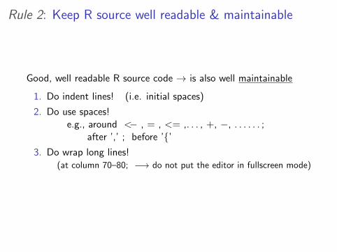
Rule 2: Keep R source well readable & maintainable

Good, well readable R source code → is also well maintainable

1. Do indent lines! (i.e. initial spaces)

2. Do use spaces!e.g., around <− , = , <= ,. . . , +, −, . . . . . . ;

after ’,’ ; before ’{’3. Do wrap long lines!

(at column 70–80; −→ do not put the editor in fullscreen mode)

well maintainable (Rule 2 cont.)

4. Do use comments copiously! (about every 10 lines)We recommend

‘##’ for the usually indented comments,‘#’ for end-of-line comments, and‘###’ for the (major) “sectioning” or beginning-of-line

ones.

5. Sometimes even better (but more laborious): Use Sweave orknitr (or org-mode or another “weave & tangle” system(noweb))

6. E.g., R source in R Markdown (*.Rmd) format.

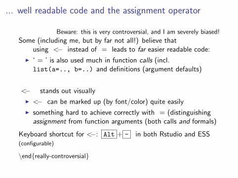
... well readable code and the assignment operator

Beware: this is very controversial, and I am severely biased!

Some (including me, but by far not all!) believe thatusing <− instead of = leads to far easier readable code:

I ‘ = ’ is also used much in function calls (incl.list(a=.., b=..) and definitions (argument defaults)

<− stands out visually

I <− can be marked up (by font/color) quite easily

I something hard to achieve correctly with = (distinguishingassignment from function arguments (both calls and formals)

Keyboard shortcut for <−: Alt + - in both Rstudio and ESS(configurable)

\end{really-controversial}

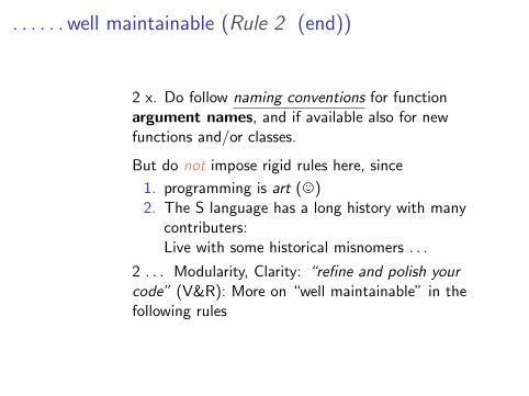
. . . . . . well maintainable (Rule 2 (end))

2 x. Do follow naming conventions for functionargument names, and if available also for newfunctions and/or classes.

But do not impose rigid rules here, since

1. programming is art (,)2. The S language has a long history with many

contributers:Live with some historical misnomers . . .

2 . . . Modularity, Clarity: “refine and polish yourcode” (V&R): More on “well maintainable” in thefollowing rules

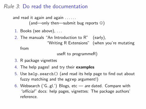
Rule 3: Do read the documentation

and read it again and again . . . . . .(and—only then—submit bug reports ,)

1. Books (see above), . . .

2. The manuals “An Introduction to R” (early),“Writing R Extensions” (when you’re mutating

fromuseR to programmeR)

3. R package vignettes

4. The help pages! and try their examples

5. Use help.search() (and read its help page to find out aboutfuzzy matching and the agrep argument!)

6. Websearch (‘G..gl.’) Blogs, etc — are dated. Compare with“official” docs: help pages, vignettes: The package authors’reference.

Rule 4: Do learn from the masters

An art is learned from the master artists:Picasso, Van Gogh, Gauguin, Manet, Klimt . . .John Chambers, Bill Venables, Bill Dunlap, Luke Tierney, BrianRipley, R-core in general :-), Dirk Eddelbuettel, Hadley Wickham. . .

Read others’ source — Learning by examples

. . . learn from the masters – Read the Source:

Obi-Wan Kenobi . . . :“Use the source, Luke!”

> install.packages("fortunes")

> fortune(250)

As Obi-Wan Kenobi may have said in Star Wars: "Use the source,

Luke!"

-- Barry Rowlingson (answering a question on the

documentation of some implementation details)

R-devel (January 2010)

Reading Source for ’?’ . . .→ Find Easter egg

> Anybody ? there ???

?

’’

(Demo)

Contacting Delphi...the oracle is unavailable.

We apologize for any inconvenience.

Read the source – of packages

I Note: The R source of an R package (in source state) is inside〈pkg〉/R/*.R, and not what you get when you display thefunction in R(by typing its name).

I R FAQ 7.40 How do I access the source code for a function?−→ Uwe Ligges (2006), “Help Desk: Accessing the sources”,

R News, 6/4, 43–45

(http://CRAN.R-project.org/doc/Rnews/Rnews_2006-4.pdf)

I Download the source package, 〈pkg〉 〈n.m〉.tar.gz typicallyfrom CRAN, unpack it and

I read it,I experiment with it, andI learn from it,

I Or browse the package source code on R-forge or github, or. . .

Rule 5: Do not Copy & Paste !

because the result is not well maintainable:Changes in one part do not propagate to the copy!

1. write functions instead

2. break a long function into several smaller ones, if possible

3. Inside functions : still Rule 5: “Do not Copy & Paste !!”−→ write local or (package) global helper functions−→ use many small helper functions (nicely hidden inNAMESPACE).

“Use functions”, e.g., use

1 mat [ c o m p l i c a t e d , compcomp ] <−i f (A) A . e x p r e l s e B . e x p r

instead of

i f (A) mat [ c o m p l i c a t e d , compcomp ] <− A . e x p r2 e l s e mat [ c o m p l i c a t e d , compcomp ] <− B . e x p r

Use Functions

Everything you do in R is calling functions anyway: In R,

Everything that exists is an object;Everything that happens is a function call.

(John Chambers — this morning, first two of three principles)

Quiz:

When if(*) ... is regarded as function with threearguments, the last being optional with a default,What is the default?

i f (C) A2 i f (C) A e l s e B

Answer: NULL: if (FALSE) A returns NULL invisibly

Rule 6: Strive for clarity and simplicity

first! . . . and second . . . and again, e.g.,think about naming of intermediate results with “self-explainable”variable namesbut use short names (plus comments) for formulae

Venables & Ripley:“Refine and polish your code in the same way you wouldpolish your English prose”

(prose: using as “dictionary” your reference material)

−→ modularity (“granularity”)

Optimization: much much later, see below

Rule 7: Test your code!

1. Carefully write (small) testing examples, for each function(“modularity”, “unit testing”)

2. Next step: Start a ’package’ via package.skeleton(). Thisallows (via R CMD check )

I auto-testing (all the help pages examples).use example(your function )

I specific testing (in a ./tests/ subdirectory, with or withoutstrict comparison to previous results)

I documenting your functions (and data, classes, methods):takes time, but almost always leads you to improve your code !

Test your code! (Rule 7 cont.)

3. Use software tools for testing:I Those of R CMD check are in the standard R package tools,

andcodetools (by Luke Tierney)

I Unit testing by packages, RUnit, testthat, etc.

After Testing, maybe Optimizing

Citing from V&R’s “S Programming” (p.172):

Jackson “Principles of Program Design” (on ‘codeoptimization’):

I Rule 1 Don’t do it.I Rule 2 (for experts only) Don’t do it yet—not until

you have a perfectly clear and unoptimized solution.

‘to the right problem by an efficient method’.

Premature optimization is the root of all evil – Donald Knuth

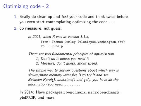
Optimizing code - 2

1. Really do clean up and test your code and think twice beforeyou even start contemplating optimizing the code . . .

2. do measure, not guess:

In 2001, when R was at version 1.1.x,

From: Thomas Lumley (tlumley@u.washington.edu)

To : R-help

There are two fundamental principles of optimisation1) Don’t do it unless you need it2) Measure, don’t guess, about speed.

The simple way to answer questions about which way isslower/more memory intensive is to try it and see.Between Rprof(), unix.time() and gc(), you have all theinformation you need. . . . . . . . . .

In 2014: Have packages rbenchmark, microbenchmark,pbdPROF, and more.

Seven Guidelines (“Rules”) – still relevant

1. Work with Source files

2. Keep R source code well readable and maintainable

3. Do read the documentation

4. Do learn from the masters — Read R (package) sources

5. Do not Copy & Paste! — Modularize into (small) Functions

6. Strive for clarity and simplicity

7. Test your code — and test, and test!

New Guidelines:

8. Maintain R code in Packages (extension of “Test!”)

9. → Source code management, e.g., subversion(svn) orgithub(git)

10. Rscript or R CMD BATCH 〈mysource〉.R should “always”work!

−→ Reproducible Data Analysis and ResearchI → Do not use .RData no, really, not ever! . . .I Rather, use save() explicitly only for expensive parts.I Consider attach("myStuff.rda") instead of

load("myStuff.rda")I Use the following outline:

s a v e f i l e <− "<myThings >.rda"

2 i f ( f i l e . e x i s t s ( s a v e f i l e ) ) attach ( s a v e f i l e ) e l s e {. . . . . . . .

4 . . . . . . . .save ( o1 , o2 , . . . , o . n , f i l e = s a v e f i l e )

6 }

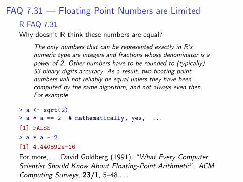
FAQ 7.31 — Floating Point Numbers are Limited

R FAQ 7.31Why doesn’t R think these numbers are equal?

The only numbers that can be represented exactly in R’snumeric type are integers and fractions whose denominator is apower of 2. Other numbers have to be rounded to (typically)53 binary digits accuracy. As a result, two floating pointnumbers will not reliably be equal unless they have beencomputed by the same algorithm, and not always even then.For example

> a <- sqrt(2)

> a * a == 2 # mathematically, yes, ...

[1] FALSE

> a * a - 2

[1] 4.440892e-16

For more, . . . David Goldberg (1991), “What Every ComputerScientist Should Know About Floating-Point Arithmetic”, ACMComputing Surveys, 23/1, 5–48.. . .

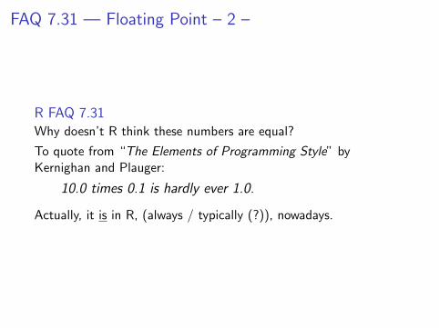
FAQ 7.31 — Floating Point – 2 –

R FAQ 7.31Why doesn’t R think these numbers are equal?

To quote from “The Elements of Programming Style” byKernighan and Plauger:

10.0 times 0.1 is hardly ever 1.0.

Actually, it is in R, (always / typically (?)), nowadays.

FAQ 7.31 ++ : The ”log” in the dpq-functions

All “dpq” distribution functions in R, i.e. density cumulativeprobability and quantile functions, have a log or log.p argument(FALSE / TRUE).

Why ?

−→ Compute Likelihoods via d<foo>(*, log = TRUE)

−→ Probalistic Networks, MC(MC): P = P1 · P2 · · · · · Pn quicklyunderflows to zero.

Solution: Work in “log space”: logP =∑

j logPj , where logPj

are computed via R’s d〈foo〉(*, log=TRUE) or p〈foo〉(*,log.p=TRUE), rather than taking logs

FAQ 7.31 . . . Why R needs even more functions

1. log1p() (since R 1.0.0), expm1() (since R 1.5.0)

Why log(1 + x) is not good enough, but log1p(x) is1 + x cannot be numerically accurate when |x| � 1. In doubleprecision (53 bits ≈ 16 digits) accuracy, 1 + x “sees” only 2–3digits of x when x = 10−14,> u <- 1 + (e <- 4e-13/9) ## then u - 1 == e mathematically:

> rbind(‘u-1‘ = u - 1, e)

[,1]

u-1 4.440892e-14

e 4.444444e-14

And the consequence for log(1 + x),> curve(abs(1 - log(1+x) / log1p(x)), 1e-17, .2, log = ’xy’, main = "..", ..)

> sfsmisc :: eaxis(1); eaxis(2)| relative error of log(1+x) |

x

10−17 10−15 10−13 10−11 10−9 10−7 10−5 10−3 10−1

10−1610−1410−1210−1010−810−610−410−2100

Why log1p(x) beats log(1 + x)

| relative error of log(1+x) |

x

10−17 10−15 10−13 10−11 10−9 10−7 10−5 10−3 10−1

10−1610−1410−1210−1010−810−610−410−2100

Solution: Expand log(1 + x) around x = 0. Well known

log(1 + x) = x− x2/2 + x3/3± . . . =∞∑n=1

(−1)n+1xn

n,

for |x| < 1.

Fast version of this expansion: typically used in log1p().

FAQ 7.31 . . . Why R needs even more functions –2–

2. cospi(), sinpi(), tanpi() (from R 3.2.0), e.g.,

cospi(x):= cos(π · x), accurately, e.g., for x = 12 :

> cos(pi/2) ## mathematically == 0

[1] 6.123234e-17

> cospi(1/2)

[1] 0

3. log1mexp() . . . (my research; in R’s Rmathlib C code, nameddiffer.)

Simple (semi-artificial!) Example: logit(exp(-L))Logistic regression: Computing “logit()”s, log p

1−p accurately forvery small p, i.e., p = exp(−L), or

logp

1− p= log p− log(1− p) = −L− log(1− exp(−L)),

and hence − log(1− exp(−L)) is needed, e.g., when p is reallyreally close to 0, say p = 10−1000, as then we can only computelogit(p), if we specify L := − log(p)↔ p = exp(−L).> curve(-log(1 - exp(-x)), 0, 10)

0 2 4 6 8 10

0.0

1.0

2.0

x

−lo

g(1

− e

xp(−

x))

seems fine. — — However, . . .

However, further out to 50 (and on a log scale), we observe

0 10 20 30 40 50

x

−lo

g(1

− e

xp(−

x))

10−16

10−8

100

early underflow to 0

which shows early underflow.

What did happen? Look at> x <- -40:-35

> -log(1 - exp(x))

[1] 0.000000e+00 0.000000e+00 0.000000e+00 1.110223e-16 2.220446e-16

[6] 6.661338e-16

> log(-log(1 - exp(x)))# --> -Inf values

[1] -Inf -Inf -Inf -36.73680 -36.04365 -34.94504

> ## ok, how about more accuracy

> x. <- mpfr(x, 120)

> log(-log(1 - exp(x.)))# aha... looks perfect now

6 ’mpfr’ numbers of precision 120 bits

[1] -39.999999999999999997932904877538241734

[2] -38.99999999999999999423372196756935807

[3] -37.99999999999999998430451715981029611

[4] -36.999999999999999957331848579613165434

[5] -35.999999999999999884024061830552087239

[6] -34.999999999999999684744214015307532692

Visually, and with “high accuracy” mpfr-numbers:> x <- seq(-40, -20, by = .5)

> plot(x,x, type="n", ylab="", ann=FALSE)

> lines(x, log(-log(1 - exp(x))), type = "o", col = "purple", lwd=3, cex = .6)

> x. <- mpfr(x, 120)

> lines(x, log(-log(1 - exp(x.))), col=2, lwd=1.5)

−40 −35 −30 −25 −20

−40

−35

−30

−25

−20

● ●

●●

●●

●

●

●

●

●

●

●

●

●

●

●

●

●

●

●

●

●

●

●

●

●

●

●

●

●

●

●

●

●

The “real” solution uses a piecewise implementation oflog1mexp(x) = log(1− exp(−x)) for x > 0, see e.g., R packagecopula.

Specific Hints, Tips:

1. Subsetting (“[ .. ]”):

1.1 Matrices, arrays (& data.frames):Instead of x[ind ,], use x[ind, , drop = FALSE] !

1.2 tricky because of NAsInside “[ .. ]”, often use %in% (wrapper of match()) orwhich().

2. Not x == NA but is .na(x)

3. Use ’1:n’ only when you know that n is positive:Instead of 1:length(obj), use seq along(obj)

Specific Hints – 2:

4. Do not grow objects:If you cannot avoid a for loop, replace

rmat <− NULL2 f o r ( i i n 1 : n ) {

rmat <− rb ind ( rmat , l o n g . computat ion ( i , . . . . . ) )4 }

byrmat <− matrix ( 0 . , n , k )

2 f o r ( i i n 1 : n ) {rmat [ i , ] <− l o n g . computat ion ( i , . . . . . )

4 }

and almost always, column by column instead of row by row(creating the transpose):

tmat <− matrix ( 0 . , k , n )2 f o r ( i i n 1 : n ) {

tmat [ , i ] <− l o n g . computat ion ( i , . . . . . )4 }

Specific Hints, Tips (cont.)

5. Use lapply(), sapply(), sometimes preferably vapply()mapply() (Apply to multiple arguments), or sometimes thereplicate() wrapper:

sample <− r e p l i c a t e (1000 , median ( r t (100 , df =3)))2 h i s t ( sample )

6. Use with(<d.frame>, ......) and do not attach dataframes

7. Use TRUE and FALSE, not ‘T’ and ‘F’ !

8. know the difference between ‘|’ vs ‘||’ and ‘&’ vs ‘&&’and inside if ( .... ) almost always use ‘||’ and ‘&&’!

9. use which.max(), . . . , findInterval()

10. Learn about ‘Regular Expressions’: ?regexp etc

What Style is your R programming?Perform the art, enjoy and be productive!

Martin.Maechler@R-project.org