GOLD PRICE TARGETING BY THE FED∗

William D. LastrapesAssociate Professor

and

George SelginAssistant Professor

Department of EconomicsUniversity of GeorgiaAthens, Georgia 30602

July 1995

Corresponding Author: William D. Lastrapes, Department of Economics, Univer-sity of Georgia, Athens, GA 30602. Phone: 706/542-3569. Fax: 706/542-3376. E-mail:last@rigel.econ.uga.edu.

William D. Lastrapes George SelginAssociate Professor Assistant ProfessorDepartment of Economics Department of EconomicsUniversity of Georgia University of GeorgiaAthens, GA 30602 Athens, GA 30602

ABSTRACT

This paper estimates a vector autoregression using weekly data to identify the response

of monetary policy to the price of gold. A simple model of the reserve market is used to

identify economic shocks. We find that over Greenspan’s tenure as Board chairman of the

Federal Reserve System, the evidence is consistent with gold price stabilization, although

the response of nonborrowed reserves to gold price shocks is strongest over intermediate

horizons. The evidence for the use of gold as an intermediate target is much weaker for

the period prior to Greenspan’s appointment. These results hold even when alternative

informational variables are considered.

JEL classification: E4, E5

1. Introduction

What role does the price of gold play in formulating current monetary policy? Fed

Chairman Alan Greenspan has called the price of gold a “very good indicator of future

inflation,” and there has long been speculation in the popular press (e.g. Forbes 1991,

Ullmann 1994) concerning a role for the gold price as an intermediate monetary policy

target: the Federal Reserve responds to changes in the price of gold in the short-run

because it cannot afford to wait for lower-frequency information concerning changes in

the aggregate variable (e.g. the price level) whose value it ultimately wishes to control.

Thus, the Fed is supposed to interpret a rising gold price as indicative of excess liquidity

or inflationary expectations, in which case the Fed reduces bank reserves to stabilize gold’s

price. Here we examine this claim empirically by focusing on the narrow question: how

does monetary policy, as measured by changes in nonborrowed reserves and the federal

funds rate, dynamically respond to independent changes in the price of gold?

To this end, we consider a linear, time series model of reserve market variables and the

price of gold. We identify, without severely restricting dynamic relationships, economic

shocks of interest by imposing a contemporaneous structural model of reserve market

behavior, similar to Strongin’s (1992), on the statistical model. Using high frequency

(weekly) data for the recent period over which the Fed has targetted borrowed reserves,

we estimate the dynamic response of the Fed’s policy instruments – nonborrowed reserves

and the funds rate – to gold price shocks.

Surprisingly, there has been little empirical research on the relationship between gold

prices and monetary policy under fiat money regimes. Many writings have, of course,

looked into the workings of gold standard regimes; others have studied the efficiency of

the market for gold (Moore 1990, Solt and Swanson 1981) and the statistical properties

of gold price time series (Frank and Stengos 1989). However, while some more recent

VAR studies of monetary policy include monthly commodity price indices (e.g. Cody

and Mills 1991, Furlong 1989, Gordon and Leeper 1994), these and earlier studies of the

Fed’s reaction function (e.g. Khoury 1990) do not include gold prices. Laurent (1994)

looks at gold in the context of monetary policy, but takes a normative perspective on the

desirability of stabilizing gold under a fiat standard, and does not investigate whether any

link actually exists between the gold price and monetary policy. Our study attempts to

provide additional insight into the mechanics of monetary policy behavior by relating gold

to policy variables using weekly data.

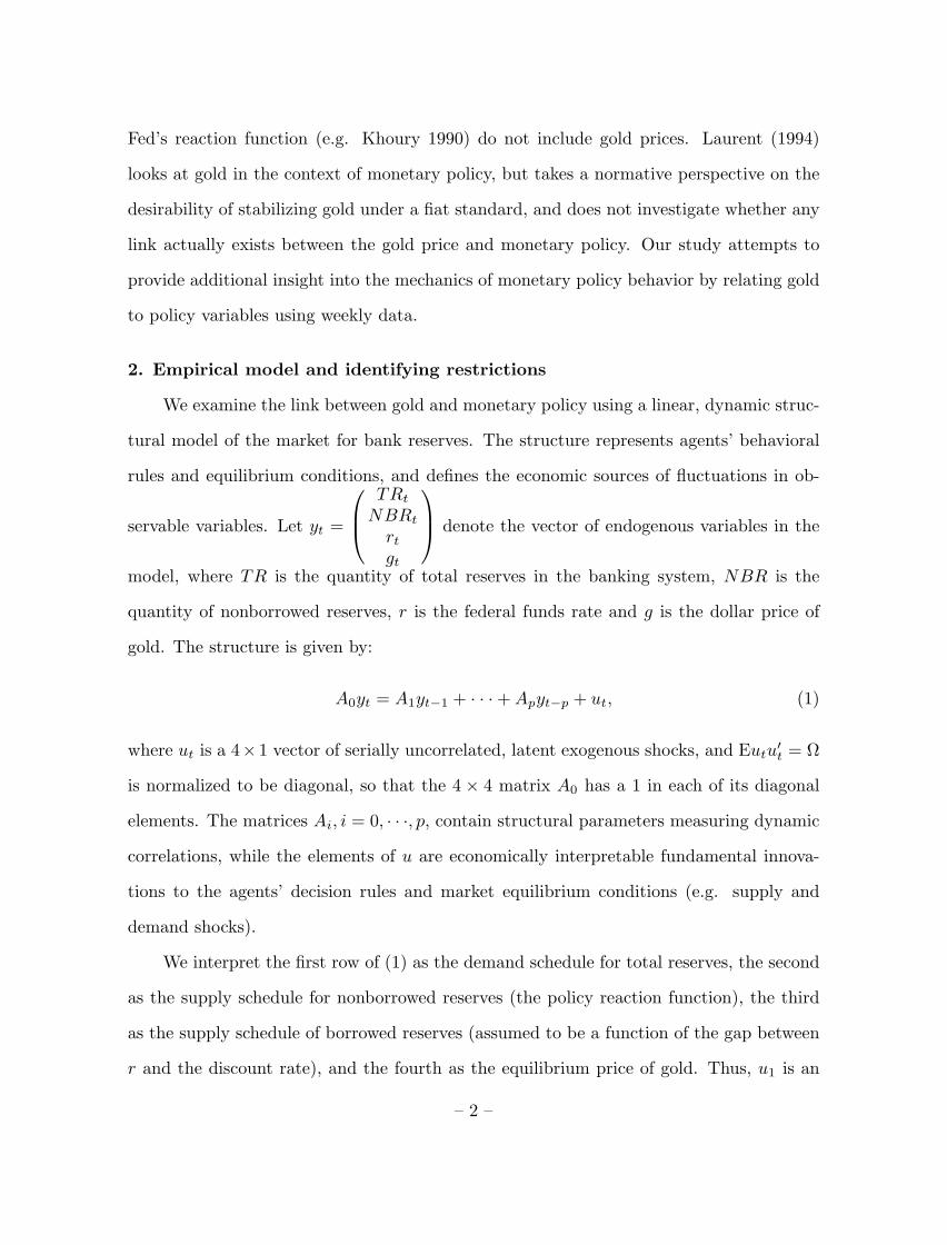
2. Empirical model and identifying restrictions

We examine the link between gold and monetary policy using a linear, dynamic struc-

tural model of the market for bank reserves. The structure represents agents’ behavioral

rules and equilibrium conditions, and defines the economic sources of fluctuations in ob-

servable variables. Let yt =

TRt

NBRt

rtgt

denote the vector of endogenous variables in the

model, where TR is the quantity of total reserves in the banking system, NBR is the

quantity of nonborrowed reserves, r is the federal funds rate and g is the dollar price of

gold. The structure is given by:

A0yt = A1yt−1 + · · ·+Apyt−p + ut, (1)

where ut is a 4×1 vector of serially uncorrelated, latent exogenous shocks, and Eutu′t = Ω

is normalized to be diagonal, so that the 4 × 4 matrix A0 has a 1 in each of its diagonal

elements. The matrices Ai, i = 0, · · ·, p, contain structural parameters measuring dynamic

correlations, while the elements of u are economically interpretable fundamental innova-

tions to the agents’ decision rules and market equilibrium conditions (e.g. supply and

demand shocks).

We interpret the first row of (1) as the demand schedule for total reserves, the second

as the supply schedule for nonborrowed reserves (the policy reaction function), the third

as the supply schedule of borrowed reserves (assumed to be a function of the gap between

r and the discount rate), and the fourth as the equilibrium price of gold. Thus, u1 is an

– 2 –

exogenous innovation to total reserve demand, u2 is a monetary policy innovation that is

independent of the other variables in the system, u3 is a shock to the supply of borrowed

reserves (which is tantamount to a shift in bank demand for Fed discount loans), and u4 is

a shock to the equilibrium gold price. The main objective of this paper is to identify the

dynamic response of the Fed to changes in u4 to make inferences about the relationship

between monetary policy and the gold price.

Dynamic responses are obtained by “solving” the structural model:

yt = (D0 +D1L +D2L2 + · · ·)ut = D(L)ut, (2)

where D0 = A−10 is nonsingular, and D(L) = (A0 − A1L − A2L2 − · · · − ApLp)−1. Thus,

Dk = ∂yt

∂ut−k. These dynamic multipliers show the average impact of an exogenous structural

impulse at time t−k on the equilibrium values of the endogenous variables at time t. If the

Fed attempts to stabilize the gold price, the reserve market should tighten in the face of

exogenous positive gold price impulses. This would imply that ∂NBRt

∂u4t−k< 0 and ∂rt

∂u4t−k> 0.

The dynamics of the policy response depend on how these multipliers vary over k.

The correspondence between D(L) and the data generating process is not unique.

This process is:

yt = (I + C1L + C2L2 + · · ·)εt = C(L)εt (3)

Eεtε′t = Σ,

which fully summarizes the second moments of the joint probability distribution of yt.

C(L) and Σ are directly recoverable from the vector autoregressive (VAR) representation

of the data. The mapping between (3) and the structure is given by

C(L) = D(L)D−10 (4)

εt = D0ut.

Clearly, this mapping can only be made unique by imposing further restrictions on the

structure.

– 3 –

To identify D(L), the parameters of interest, from C(L), we do not restrict dynamic

interactions by imposing strict econometric exogeneity on the variables in the system, but

focus on the information contained in the covariance of the residuals from an unrestricted

VAR, Σ. Note from (3) and (4) that

Σ = D0ΩD′0. (5)

Because Σ is symmetric, there are ten independent, nonlinear relations between the es-

timable elements in Σ and the sixteen structural parameters in D0 (or A0) and Ω. Six

restrictions are required on the structure to just-identify these parameters. Note again

from (4) that knowledge of D0 is sufficient to estimate D(L).

The restrictions we impose are based on a simple model of contemporaneous interac-

tion of the variables in yt, which restricts the elements of A0. The model is not recursive,

so that the Choleski decomposition of Σ is not an appropriate identifying scheme.1 The

model implies:

A0 =

1 0 0 0a21 1 a23 a24

a31 −a31 1 00 a42 a43 1

. (6)

The zero restrictions in the first row of A0 (a12 = a13 = a14 = 0) imply that the

demand for reserves by depository institutions is perfectly inelastic with respect to the

current federal funds rate and does not respond contemporaneously to changes in the other

variables; thus, u1 is simply the reduced form innovation from the total reserves equation.

These restrictions do not rule out adjustment of reserves over time and therefore allows

for an elastic demand at longer horizons.

Strongin (1992) makes a similar identifying restriction and provides a rationalization

for why banks’ demand for reserves might be independent of interest rates and supply

factors in the short run. In particular, the restriction relies on two institutional rigidities:

1) required reserve demand is predetermined by current and past deposits, the demand for

which is inelastic in the short-run; and 2) excess reserve demand is independent of policy.

– 4 –

These rigidities are a fortiori more plausible over a weekly horizon than in Strongin’s

monthly horizon application.

As noted above, the second row reflects the policy behavior of the central bank. We

impose no restrictions on how the Fed responds to contemporaneous movements in total

reserves, the federal funds rate, or the price of gold. This specification is sufficiently general

to allow for any targetting or policy procedure undertaken by the Fed. For example, under

a pure borrowed reserves procedure, the Fed immediately accommodates reserve demand

shocks; thus, a21 = −1. If the Fed targets the federal funds rate by smoothing private

sector shocks to borrowed reserves, then a23 < 0. If a24 > 0, the Fed reduces nonborrowed

reserves in response to an increase in gt and thus (assuming that the price of gold is

perceived to respond positively to increases in money) attempts to stabilize the price of

gold contemporaneously. Regardless of the particular procedure chosen by the Fed, u2 is

a policy shock that does not depend on feedback from the other variables in the system;

it is the only sort of shock that can tell us how exogenous monetary policy is transmitted

to the real economy (Christiano, Eichenbaum and Evans 1994).

Two restrictions are placed on the third row, the borrowed reserve supply equation:

a32 = −a31, which defines borrowed reserves, and a34 = 0, which implies that borrowed

reserve supply is independent of the gold price. Recall that u3 represents shocks to factors

other than the federal funds rate that influence the desire for borrowed reserves, such as

the implicit costs and benefits of utilizing the discount window (Thornton 1988). When

u3 > 0, borrowed reserve supply decreases for a given federal funds rate (it represents an

increase in the cost of borrowing from the Fed relative to borrowing in the federal funds

market).

In the final row – the reduced form equation for gold (where the supply and demand

for gold implicitly have been solved for price by eliminating quantity) – the only restric-

tion imposed is that total reserves may affect the demand for gold, but only with a lag.2

A negative value for a42 implies that increases in reserve market liquidity lead to a con-

– 5 –

temporaneous increase in the demand for, and therefore price of, gold. The shock u4 can

include shocks to inflationary expectations that affect the demand for gold but that come

from information external to the reserve market.

The six restrictions in A0 are sufficient to just-identify D0 and thus D(L) from the

VAR estimates of Σ (assuming the rank condition for identification holds). Keep in mind

that these restrictions are contemporaneous and do not place theoretical restrictions on

dynamic interactions.

3. Results

Our statistical analysis focuses on Greenspan’s tenure as chairman of the Fed, be-

ginning in August 1987. Operating procedures have been fairly stable over this period,

with price level stability arguably being the Fed’s sole long-run (or ultimate) objective

(Timberlake, 1993, pp. 390-401). However, we also estimate the model over the borrowed

reserve period prior to Greenspan’s appointment, beginning in October 1982, to see if

Greenspan’s appointment has affected the Fed’s response to gold. In addition, we consider

the robustness of the results to potential omitted variable problems.

The full sample contains weekly observations of the reserve market and gold price

variables from October 6, 1982 to April 27, 1994. The subsample spanning Greenspan’s

term begins August 11, 1987. The pre-Greenspan subsample begins October 6, 1982 and

end August 5, 1987. Weekly data allow us to examine the possibility that the Fed re-

sponds quickly to asset price changes. They also enhance the plausiblity of the model’s

identifying restrictions. The data set consists of the adjusted monetary base (Wednesday),

the currency component of M1 (Tuesday), total borrowings from the discount window

(Wednesday), and the federal funds rate (Wednesday). Total reserves are measured as

the difference between the monetary base and currency holdings, while nonborrowed re-

serves are obtained by subtracting borrowings from total reserves.3 The gold price is the

Wednesday close from Comex.

– 6 –

Over both samples, we estimate a VAR with a common lag of 15, which sufficiently

whitens the residuals. To allow for these lags, the first 15 observations are taken as

given, so that the estimation period begins January 26, 1983 (237 observations) for the

early subsample and December 2, 1987 (335 observations) for the Greenspan subsample.

Deterministic variables include a constant and the Fed discount rate. All variables in

the system except the federal funds rate are transformed into logs.4 We use a two-step

procedure to efficiently estimate the structural parameters. In the first step, OLS equation-

by-equation yields Σ. In the second step, maximizing the log likelihood

L(Σ, A0,Ω) = −Tn2log2π +

T

2log|A0|2 −

T

2log|Ω| − T

2trace[(A′0Ω−1A0)Σ] (7)

with respect to A0 and Ω yields (assuming they are identified) the FIML estimators of

these parameters, A0 and Ω (Hamilton 1994). Because our restrictions just-identify the

system, Σ = A0−1

Ω(A0−1

)′, and there are no over-identifying restrictions to test.

Figures 1 and 2 report the dynamic response functions, where the responses are scaled

to a standard deviation impulse to each shock, and the variance decompositions of the vari-

ables, estimated over the Greenspan subsample. Each figure also shows asymmetric stan-

dard error bands obtained from a bootstrap simulation. The bands give some indication

of the precision of the estimates.5

Consider the first column of panels in the figures. In Figure 1, this column shows the

average dynamic response of each of the system variables to an impulse in the demand

for reserves. The results are consistent with a borrowed reserve operating procedure:

nonborrowed reserves track the movement in total reserves closely, meaning that borrowed

reserves do not respond to demand shocks. The response of the federal funds rate is

essentially zero, with virtually no contribution of reserve demand shocks to the variance

of the rate.

Column two reports the responses to exogenous monetary policy shocks. A u2 shock

that has a positive impact effect on nonborrowed reserves causes a decline in the federal

– 7 –

funds rate: a shock causing a 1% increase (measured on a weekly basis) in nonborrowed

reserves on impact brings about an average decline in the federal funds rate of 30.67 basis

points. This finding is further evidence for a liquidity effect of nominal money shocks,

which has recently been a focus of several empirical studies (Lastrapes and Selgin 1994,

Christiano and Eichenbaum 1992a,b, Strongin 1992, Gordon and Leeper 1994).6 Such

shocks on average explain about 50% of the variance of the federal funds rate at a one-

week horizon and beyond. The rate response is surprisingly persistent given the apparent

transitory nature of the shock on non-borrowed reserves and the lack of an effect on total

reserves. The positive response of gold price to the policy shock is also somewhat surprising

given the small effect of the shock on reserves. However, the contribution of the shock to

gold price variance is relatively small.

The results in column three suggest that an increase in the implicit costs of discount

borrowing has a transitory but strong effect on the federal funds rate. This, coupled with

the essentially zero response of nonborrowed reserves, suggests that the Fed is reluctant to

smooth the federal funds rate in the face of borrowed reserve shocks.7

Responses to exogenous gold price shocks are reported in column four. (For clarity,

Figure 3 contains these response functions only, without standard error bands.) There is

clear evidence of market tightening in response to positive innovations in the price of gold.

Although the response is weak initially, non-borrowed reserves gradually fall as the federal

funds rate rises. Total reserves do not respond over short-horizons, but eventually fall as

the demand for reserves becomes elastic and the federal funds rate rises. Furthermore, if the

nonborrowed reserve response were simply an accommodation of a gold-induced leftward

shift in the demand for reserves, the federal funds rate response would be negative rather

than positive. According to the variance decompositions, gold price shocks explain 25%

of the 52-week forecast error variance of nonborrowed reserves, and 41% of the variance

of the federal funds rate at that horizon. Finally, note that the gold price itself responds

only temporarily to its own shocks. This finding is also consistent with long-run gold price

– 8 –

stabilization – after 52 weeks, gold’s response to u4 is only one-eighth of its immediate

response.8

Though modest, the magnitudes of these intermediate-horizon responses of policy

variables are not trivial: a shock to u4 that causes a 10% rise in the price of gold on

impact brings about a 1.5% fall in nonborrowed reserves and a 50.7 basis point rise in the

federal funds rate at the 52 week horizon. In 1994, for example, this would have meant

a decline in nonborrowed reserves of about $1.6 billion. This response is larger than the

estimated standard deviation of the policy shock error of 0.60%.

Because our empirical model includes only the price of gold, it cannot distinguish the

influence of the gold price on Fed policy from the influence of other information variables

that may correlated with the gold price. For example, past studies have considered, with

mixed results, the role of commodity prices other than gold in influencing monetary policy

(Cody and Mills 1991, Furlong 1989). The price of gold might proxy for a more general

commodity price index in the Fed’s reaction function. It might also proxy for more direct

measures of the Fed’s goals, such as the price level and output.

To analyze the robustness of our results, we create three series representing a measure

of the “relative” price of gold. The first is the dollar gold price deflated by a weekly

commodity price index. The second deflates the gold price by the price level, while the

third is the ratio of gold price to output. We then estimate three separate VARs in which

the relative prices alternately replace the nominal price of gold. If the Fed attempts to

stabilise commodity prices, the price level or output directly rather than the price of gold,

then nonborrowed reserves should respond positively to an exogenous shock in the relative

price measure.9

Figure 4 plots the dynamic responses of the system variables to these relative gold

price shocks estimated over the Greenspan period. The basic patterns of the responses

of the reserve market variables to these shocks are unchanged. In particular, there is no

tendency for the Fed to expand reserves following a relative decrease in the variable in

– 9 –

the denominator of the relative price variable. The unreported response functions are also

robust. These results do not rule out a role for other commodity prices, the price level or

output in setting monetary policy. They do suggest, nonetheless, that gold plays a larger

role in the setting of policy than either the commodity price index or the less-frequently

observed aggregate variables.10

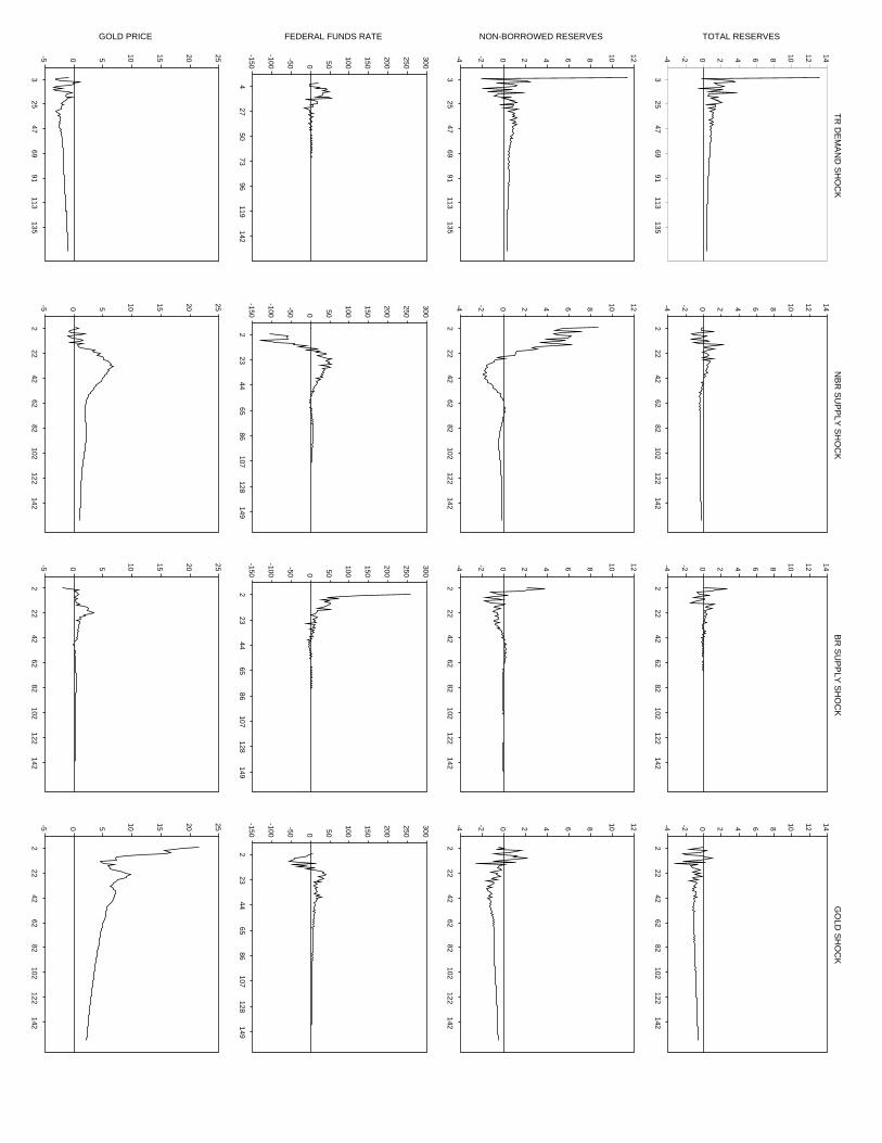
Figures 5 and 6, finally, show the response functions and variance decompositions for

the original system estimated over the pre-Greenspan subsample. The primary finding

of reserve tightening in response to positive gold price shocks is much less evident before

Greenspan. Note the weaker response of both nonborrowed reserves and the federal funds

rate in column 4. In fact, the federal funds rate declines over short horizons. Both figures

indicate that exogenous policy shocks (u2) are more persistent and explain much more of

the variation in nonborrowed reserves.11 We infer that targeting the price of gold has been

more important during Greenspan’s tenure as Board Chairman than during the borrowed

reserve period prior to his appointment.

4. Conclusion

In this paper, we statistically investigate the response of monetary policy to move-

ments in the price of gold, taking care to appropriately identify policy reactions and to

account for dynamic relationships. The results of this empirical exercise confirm the

widespread belief that Alan Greenspan’s Fed has used the price of gold to guide mon-

etary policy over medium-term horizons: the responses of nonborrowed reserves and the

federal funds rate to gold price shocks are gradual and peak between 26 and 40 weeks.

The inclusion of other potential target variables – commodity prices, inflation and output

– in the statistical model does not alter our basic findings.

– 10 –

Notes

1 The type of contemporaneous restrictions we use were initially used to identify

VAR models by Bernanke (1986) and Sims (1986). Giannini (1992) discusses in general

identification of VAR models.2 We also identified A0 by relaxing the restriction on a41 and restricting a43 to be

zero; our results were unaffected.3 A direct measure of total reserves is available on a biweekly basis. We compared

our measure to the direct measure for this frequency – they were almost identical. Thus,

our results are not sensitive to the possible mismatch of the base and currency.4 Note that this transformation does not preserve the definition of borrowed reserves

in terms of total and nonborrowed reserves. Thus, our identification scheme is an approxi-

mation. However, we also estimated a system in which reserve variables are normalized as

in Strongin (1992) by dividing TRt and NBRt by TRt−1, and a system without normal-

ization. The results in these cases were not qualitatively different from those reported.5 The simulation proceeded as follows. A pseudo realization of yt, t = 1 · · · T was

generated using bootstrapped residuals and the initial values of the variables. With the

pseudo data, a VAR was estimated, the structural parameters were identified using (7),

and the dynamic multipliers and variance decompositions calculated. This procedure was

replicated 1000 times. However, in 201 cases, the optimization algorithm failed to converge

for a common set of starting conditions. We therefore constructed the empirical density

of the estimated coefficients over the remaining 799 replications. The standard errors

reported in Figures 1 and 2 were calculated separately for pseudo responses above, and

below, the actual estimates; hence, the asymmetry of the bands (Blanchard and Quah

1989).6 The only other studies, of which we are aware, to provide evidence of a liquidity effect

over data frequencies higher than monthly are Bernanke and Blinder 1992 and Cochrane

1989.7 For research that finds some evidence for accommodation of borrowed reserve shocks,

see Thornton (1988, pp. 42-43).8 The estimate of a24 is 0.037 with a standard error of 0.004. Thus, nonborrowed

– 11 –

reserve supply is significantly negatively related contemporaneously to changes in the price

of gold.9 We use the KR-CRB (BLS) spot commodity price index from Knight-Ridder. The

Commodity Research Bureau daily index includes 23 commodity prices, excluding gold.

As with the other data, Wednesday figures are chosen to form the weekly sample. The

price level is the consumer price index for all urban consumers, and output is the seasonally

adjusted index of industrial production. The latter two series are obtained from the Federal

Reserve Bank of St. Louis Electronic Data Base. The price level and output proxies are

converted to a weekly basis by assuming that they are constant over the month. Since

these variables are available to the Fed only on a monthly basis as well, this is a reasonable

assumption. In addition, while the monthly variables cannot effect the high frequency

responses, they can be used to determine if the longer-run responses of the reserve market

variables we estimate in the initial system overstate the case for gold.10 Greenspan himself has deemed the gold price to be a much better indicator of

inflationary expectations that other commodity prices.11 An interesting sidelight of these figures is the response of gold to policy shocks:

while the federal funds rate drops immediately, the price of gold rises more gradually when

nonborrowed reserves rise. This result is consistent with a distribution effect of money

(Fuerst 1992 and others) – the monetary impulse is first felt in the reserves market, and

later spills over into other asset markets.

– 12 –

References

Bernanke, Ben. “Alternative Explanations of the Money-income Correlation.” Carnegie

-Rochester Conference Series on Public Policy, 1986, 25, 49-100.

Bernanke, Ben and Alan Blinder “ The Federal Funds Rate and the Channels of Monetary

Transmission,” American Economic Review, September 1992, 82, 901-21.

Blanchard, Olivier J., and Danny Quah. “The Dynamic Effects of Aggregate Demand

and Supply Disturbances.” American Economic Review, September 1989, 79, 655-73.

Christiano, Lawrence J. and Martin Eichenbaum, “Identification and the Liquidity Effect

of a Monetary Shock,” in A. Cuikerman, L.Z. Hercowitz, and L. Leiderman,

eds., Business Cycles, Growth and Political Economy, Cambridge, MA: MIT Press,

1992a.

Christiano, Lawrence J. and Martin Eichenbaum, “Liquidity Effects and the Monetary

Transmission Mechanism,” American Economic Review, May 1992b, 82, 346-353.

Christiano, Lawrence J., Martin Eichenbaum, and Charles L. Evans. “The Effects of

Monetary Policy Shocks: Evidence from the Flow of Funds,” Federal Reserve Bank

of Chicago Working Paper 94-2, March 1994.

Cochrane, John H. “The Return of the Liquidity Effect: A Study of the Short-Run

Relation Between Money Growth and Interest Rates,” Journal of Business and

Economic Statistics, January 1989, 7, 75-83.

Cody, Brian J. and Leonard O. Mills. “The Role of Commodity Prices in Formulating

Monetary Policy,” The Review of Economics and Statistics, May 1991, 63, 358-65.

Forbes, Malcolm S. Jr. “Is Gold Running the Fed?” Forbes, October 14, 1991, 25.

Frank, Murray and Thanasis Stengos, “Measuring the Strangeness of Gold and Silver Rates

of Return,” Review of Economic Studies, 1989, 56, 553-67.

Fuerst, Timothy “Liquidity, Loanable Funds and Real Activity,” Journal of Monetary

Economics, 1992.

– 13 –

Furlong, Frederick T. “Commodity Prices as a Guide for Monetary Policy,” Federal Reserve

Bank of San Francisco Economic Review, Winter 1989, 21-38.

Giannini, Carlo. Topics in Structural VAR Econometrics, Springer-Verlag, 1992.

Gordon, Donald B. and Eric M. Leeper, “The Dynamic Impacts of Monetary Policy: An

Exercise in Tentative Identification,” Federal Reserve Bank of Atlanta Working Paper

93-5, April 1993.

Hamilton, James D. Time Series Analysis, Princeton, NJ: Princeton University Press,

1994.

Khoury, Salwa S. “The Federal Reserve Reaction Function: A Specification Search,” in

Thomas Mayer (editor), The Political Economy of American Monetary Policy,

Cambridge: Cambridge University Press, 1990.

Lastrapes, William D., and George Selgin “The Liquidity Effect: Identifying Short-Run

Interest Rate Dynamics using Long-Run Restrictions,” Journal of Macroeconomics,

Summer 1995, 17, 387-404.

Laurent, Robert D. “Is There a Role for Gold in Monetary Policy?” Federal Reserve Bank

of Chicago Economic Perspectives, March/April 1994, 2-14.

Moore, Geoffrey H. “Gold Prices and a Leading Index of Inflation,” Challenge, July/August

1990, 52-56.

Sims, Christopher A., “Are Forecasting Models Usable for Policy Analysis?”

Federal Reserve Bank of Minneapolis Quarterly Review, Winter 1986, 10, 2-24.

Solt, Michael E. and Paul J. Swanson. “On the Efficiency of the Markets for Gold and

Silver,” Journal of Business, 1981, 54, 453-78.

Strongin, Steven “The Identification of Monetary Policy Disturbances: Explaining the

Liquidity Puzzle,” Research Department, Federal Reserve Bank of Chicago, working

paper WP-92-27, (November 1992).

Thornton, Daniel L. “The Borrowed-Reserves Operating Procedure: Theory and

– 14 –

Evidence,” Federal Reserve Bank of St. Louis Review, January/February 1988, 70

30-54.

Ullmann, Owen. “Why Greenspan Has a Touch of Gold Fever,” Business Week, March 7,

1994, 44.

Figure 1. Dynamic Response Functions: Greenspan era (8/11/87 to 4/27/94)

Notes: Response functions are bounded by standard error bands derived from a bootstrap

simulation with 799 replications.

Figure 2. Variance Decompositions: Greenspan era (8/11/87 to 4/27/94)

Notes: Variance decompositions are bounded by standard error bands derived from a

bootstrap simulation with 799 replications.

Figure 3. Dynamic Responses to Gold Price Shock: Greenspan era (8/11/87 to 4/27/94)

Figure 4. Dynamic Responses to Relative Gold Price Shocks: Greenspan era (8/11/87 to 4/27/94)

Figure 5. Dynamic Response Functions: Prior sample (10/6/82 to 8/5/87)

Figure 6. Variance Decompositions: Prior sample (10/6/82 to 8/5/87)

TR

DE

MA

ND

SH

OC

KTOTAL RESERVES

427

5073

96119

142 -5.0

-2.5

0.0

2.5

5.0

7.5

10.0

12.5

15.0

17.5

NON-BORROWED RESERVES

427

5073

96119

142 -5.0

-2.5

0.0

2.5

5.0

7.5

10.0

12.5

15.0

17.5

FEDERAL FUNDS RATE

427

5073

96119

142 -120

-80

-40

0

40

80

120

GOLD PRICE

427

5073

96119

142 -6.0

-3.0

0.0

3.0

6.0

9.0

12.0

15.0

18.0

NB

R S

UP

PLY

SH

OC

K

222

4262

82102

122142

-5.0

-2.5

0.0

2.5

5.0

7.5

10.0

12.5

15.0

17.5

222

4262

82102

122142

-5.0

-2.5

0.0

2.5

5.0

7.5

10.0

12.5

15.0

17.5

223

4465

86107

128149

-120

-80

-40

0

40

80

120

222

4262

82102

122142

-6.0

-3.0

0.0

3.0

6.0

9.0

12.0

15.0

18.0

BR

SU

PP

LY S

HO

CK

222

4262

82102

122142

-5.0

-2.5

0.0

2.5

5.0

7.5

10.0

12.5

15.0

17.5

222

4262

82102

122142

-5.0

-2.5

0.0

2.5

5.0

7.5

10.0

12.5

15.0

17.5

223

4465

86107

128149

-120

-80

-40

0

40

80

120

222

4262

82102

122142

-6.0

-3.0

0.0

3.0

6.0

9.0

12.0

15.0

18.0

GO

LD S

HO

CK

222

4262

82102

122142

-5.0

-2.5

0.0

2.5

5.0

7.5

10.0

12.5

15.0

17.5

222

4262

82102

122142

-5.0

-2.5

0.0

2.5

5.0

7.5

10.0

12.5

15.0

17.5

223

4465

86107

128149

-120

-80

-40

0

40

80

120

222

4262

82102

122142

-6.0

-3.0

0.0

3.0

6.0

9.0

12.0

15.0

18.0

TR

DE

MA

ND

SH

OC

KTOTAL RESERVES

326

4972

95118

141 0

25

50

75

100

NON-BORROWED RESERVES

326

4972

95118

141 0

25

50

75

100

FEDERAL FUNDS RATE

326

4972

95118

141 0

25

50

75

100

GOLD PRICE

326

4972

95118

141 0

20

40

60

80

100

NB

R S

UP

PLY

SH

OC

K

222

4262

82102

122142

0

25

50

75

100

222

4262

82102

122142

0

25

50

75

100

222

4262

82102

122142

0

25

50

75

100

222

4262

82102

122142

0

20

40

60

80

100

BR

DE

MA

ND

SH

OC

K

222

4262

82102

122142

0

25

50

75

100

222

4262

82102

122142

0

25

50

75

100

222

4262

82102

122142

0

25

50

75

100

222

4262

82102

122142

0

20

40

60

80

100

GO

LD S

HO

CK

222

4262

82102

122142

0

25

50

75

100

222

4262

82102

122142

0

25

50

75

100

222

4262

82102

122142

0

25

50

75

100

222

4262

82102

122142

0

20

40

60

80

100

TOTAL RESERVES

1 5 9 13 17 21 25 29 33 37 41 45 49 53 57 61 65 69 73 77 81 85 89 93 97 101 105 109 113 117 121 125 129 133 137 141 145 149 153-2.5

-2.0

-1.5

-1.0

-0.5

0.0

0.5

1.0

1.5

NONBORROWED RESERVES

1 5 9 13 17 21 25 29 33 37 41 45 49 53 57 61 65 69 73 77 81 85 89 93 97 101 105 109 113 117 121 125 129 133 137 141 145 149 153-2.5

-2.0

-1.5

-1.0

-0.5

0.0

0.5

1.0

FEDERAL FUNDS RATE

1 5 9 13 17 21 25 29 33 37 41 45 49 53 57 61 65 69 73 77 81 85 89 93 97 101 105 109 113 117 121 125 129 133 137 141 145 149 153 -25

0

25

50

75

100

GOLD PRICE

1 5 9 13 17 21 25 29 33 37 41 45 49 53 57 61 65 69 73 77 81 85 89 93 97 101 105 109 113 117 121 125 129 133 137 141 145 149 153 -2

0

2

4

6

8

10

12

14

16

CO

MM

OD

ITY

PR

ICE

TOTAL RESERVES

117

3349

6581

97113

129145

-2.5

-2.0

-1.5

-1.0

-0.5

0.0

0.5

1.0

1.5

2.0

NONBORROWED RESERVES

117

3349

6581

97113

129145

-2.5

-2.0

-1.5

-1.0

-0.5

0.0

0.5

1.0

1.5

FEDERAL FUNDS RATE

117

3349

6581

97113

129145

-40

-20

0

20

40

60

80

"RELATIVE" GOLD PRICE

117

3349

6581

97113

129145

-5.0

-2.5

0.0

2.5

5.0

7.5

10.0

12.5

15.0

17.5

CP

I

116

3146

6176

91106

121136

151-2.5

-2.0

-1.5

-1.0

-0.5

0.0

0.5

1.0

1.5

2.0

116

3146

6176

91106

121136

151-2.5

-2.0

-1.5

-1.0

-0.5

0.0

0.5

1.0

1.5

116

3146

6176

91106

121136

151 -40

-20

0

20

40

60

80

116

3146

6176

91106

121136

151 -5.0

-2.5

0.0

2.5

5.0

7.5

10.0

12.5

15.0

17.5

OU

TP

UT

116

3146

6176

91106

121136

151-2.5

-2.0

-1.5

-1.0

-0.5

0.0

0.5

1.0

1.5

2.0

116

3146

6176

91106

121136

151-2.5

-2.0

-1.5

-1.0

-0.5

0.0

0.5

1.0

1.5

116

3146

6176

91106

121136

151 -40

-20

0

20

40

60

80

116

3146

6176

91106

121136

151 -5.0

-2.5

0.0

2.5

5.0

7.5

10.0

12.5

15.0

17.5

TR

DE

MA

ND

SH

OC

KTOTAL RESERVES

325

4769

91113

135 -4

-2

0

2

4

6

8

10

12

14

NON-BORROWED RESERVES

325

4769

91113

135 -4

-2

0

2

4

6

8

10

12

FEDERAL FUNDS RATE

427

5073

96119

142 -150

-100

-50

0

50

100

150

200

250

300

GOLD PRICE

325

4769

91113

135 -5

0

5

10

15

20

25

NB

R S

UP

PLY

SH

OC

K

222

4262

82102

122142

-4

-2

0

2

4

6

8

10

12

14

222

4262

82102

122142

-4

-2

0

2

4

6

8

10

12

223

4465

86107

128149

-150

-100

-50

0

50

100

150

200

250

300

222

4262

82102

122142

-5

0

5

10

15

20

25

BR

SU

PP

LY S

HO

CK

222

4262

82102

122142

-4

-2

0

2

4

6

8

10

12

14

222

4262

82102

122142

-4

-2

0

2

4

6

8

10

12

223

4465

86107

128149

-150

-100

-50

0

50

100

150

200

250

300

222

4262

82102

122142

-5

0

5

10

15

20

25

GO

LD S

HO

CK

222

4262

82102

122142

-4

-2

0

2

4

6

8

10

12

14

222

4262

82102

122142

-4

-2

0

2

4

6

8

10

12

223

4465

86107

128149

-150

-100

-50

0

50

100

150

200

250

300

222

4262

82102

122142

-5

0

5

10

15

20

25

TR

DE

MA

ND

SH

OC

KTOTAL RESERVES

326

4972

95118

141 0

25

50

75

100

NON-BORROWED RESERVES

326

4972

95118

141 0

25

50

75

100

FEDERAL FUNDS RATE

326

4972

95118

141 0

25

50

75

100

GOLD PRICE

326

4972

95118

141 0

25

50

75

100

NB

R S

UP

PLY

SH

OC

K

222

4262

82102

122142

0

25

50

75

100

222

4262

82102

122142

0

25

50

75

100

222

4262

82102

122142

0

25

50

75

100

222

4262

82102

122142

0

25

50

75

100

BR

SU

PP

LY S

HO

CK

222

4262

82102

122142

0

25

50

75

100

222

4262

82102

122142

0

25

50

75

100

222

4262

82102

122142

0

25

50

75

100

222

4262

82102

122142

0

25

50

75

100

GO

LD S

HO

CK

222

4262

82102

122142

0

25

50

75

100

222

4262

82102

122142

0

25

50

75

100

222

4262

82102

122142

0

25

50

75

100

222

4262

82102

122142

0

25

50

75

100