Global Warming: Is It True?

Peter Fuller

Odeliah GreeneAmanda Smith

May Zin

What is Global Warming?

Global warming is the increase in the average temperature of the

Earth's near-surface air and oceans since the mid-twentieth

century, and its projected continuation.

Data We’re Using

Our data showed monthly average

temperatures in England

from 1850-2008

Forecasting Goal

Our purpose is to explore the validity of Global Warming with

regards to temperature change in England.

Trace

20

30

40

50

60

70

60 80 00 20 40 60 80 00

TEMP

Histogram

0

20

40

60

80

100

120

30 35 40 45 50 55 60 65

Series: TEMPSample 1850:01 2008:04Observations 1900

Mean 48.79893Median 48.02000Maximum 66.74000Minimum 28.22000Std. Dev. 8.358940Skewness 0.059055Kurtosis 1.848781

Jarque-Bera 106.0244Probability 0.000000

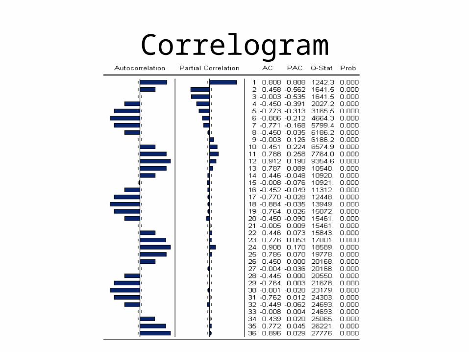
Correlogram

Unit Root TestADF Test Statistic -14.22821 1% Critical Value* -3.4368

5% Critical Value -2.8635 10% Critical Value -2.5679

*MacKinnon critical values for rejection of hypothesis of a unit root.

Augmented Dickey-Fuller Test EquationDependent Variable: D(TEMP)Method: Least SquaresDate: 06/02/08 Time: 03:02Sample(adjusted): 1850:02 2008:04Included observations: 1899 after adjusting endpoints

Variable Coefficient Std. Error t-Statistic Prob. TEMP(-1) -0.191971 0.013492 -14.22821 0.0000C 9.374922 0.668019 14.03391 0.0000R-squared 0.096427 Mean dependent var 0.006635Adjusted R-squared 0.095950 S.D. dependent var 5.168794S.E. of regression 4.914569 Akaike info criterion 6.023338Sum squared resid 45818.22 Schwarz criterion 6.029182Log likelihood -5717.159 F-statistic 202.4420Durbin-Watson stat 1.081641 Prob(F-statistic) 0.000000

How we go about fixing the data

We seasonally differenced the model using a new variable:

SDTemp=Temp-Temp(-12)

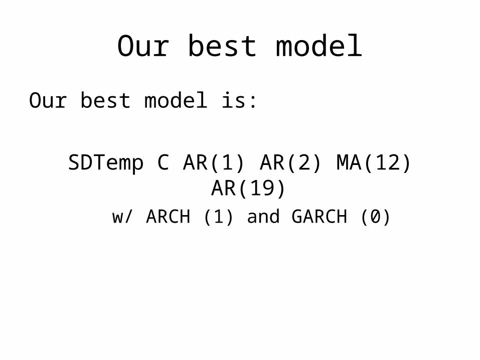
Our best model

Our best model is:

SDTemp C AR(1) AR(2) MA(12) AR(19)w/ ARCH (1) and GARCH (0)

Estimation Output

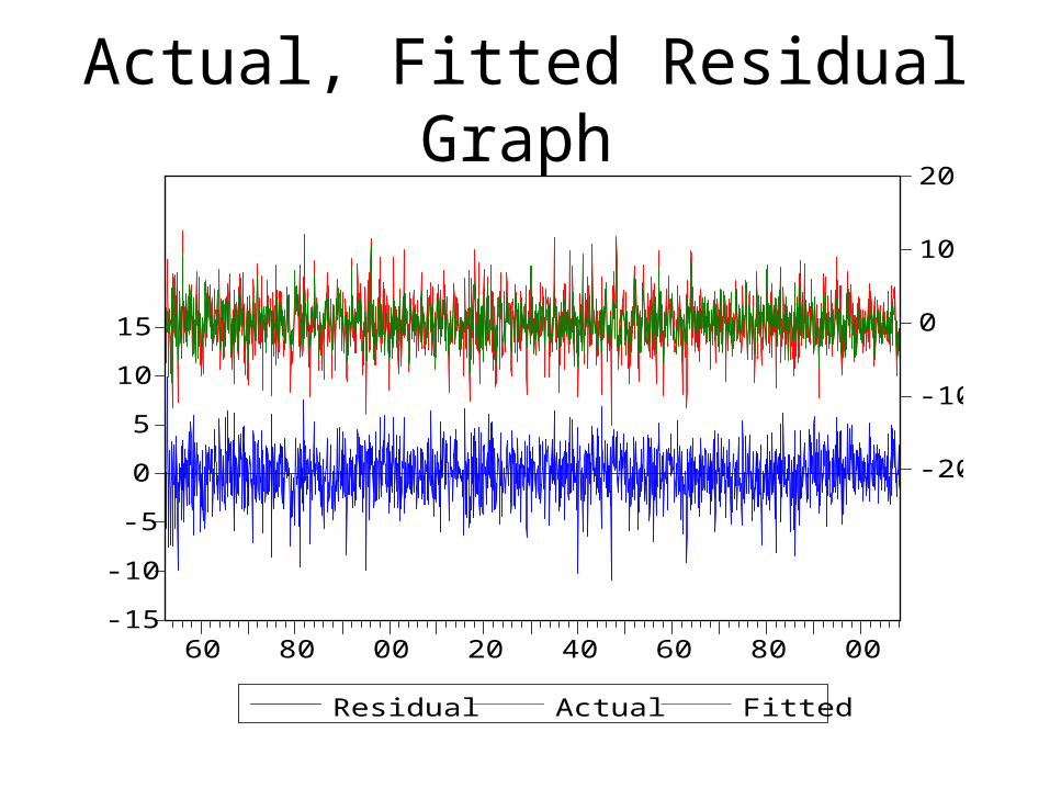
Actual, Fitted Residual Graph

-15

-10

-5

0

5

10

15

-20

-10

0

10

20

60 80 00 20 40 60 80 00

Residual Actual Fitted

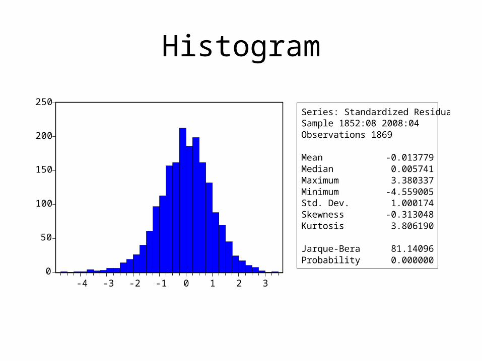
Histogram

0

50

100

150

200

250

-4 -3 -2 -1 0 1 2 3

Series: Standardized ResidualsSample 1852:08 2008:04Observations 1869

Mean -0.013779Median 0.005741Maximum 3.380337Minimum -4.559005Std. Dev. 1.000174Skewness -0.313048Kurtosis 3.806190

Jarque-Bera 81.14096Probability 0.000000

Correlogram

ARCH LM TestARCH Test:F-statistic 7.80E-05 Probability 0.992956Obs*R-squared 7.81E-05 Probability 0.992951

Test Equation:Dependent Variable: STD_RESID^2Method: Least SquaresDate: 06/02/08 Time: 03:41Sample(adjusted): 1852:09 2008:04Included observations: 1868 after adjusting endpoints

Variable Coefficient Std. Error t-Statistic Prob. C 1.000582 0.045274 22.10045 0.0000STD_RESID^2(-1) -0.0002040.023149 -0.0088300.9930R-squared 0.000000 Mean dependent var 1.000378Adjusted R-squared -0.000536 S.D. dependent var 1.681044S.E. of regression 1.681494 Akaike info criterion 3.878313Sum squared resid 5275.970 Schwarz criterion 3.884236Log likelihood-3620.344 F-statistic 7.80E-05Durbin-Watson stat 2.000032 Prob(F-statistic) 0.992956

Within Sample Forecast

-8

-6

-4

-2

0

2

4

6

05:01 05:07 06:01 06:07 07:01 07:07 08:01 08:07

SDT EMP SDT EMPF

Recoloring our Within Sample Forecast

35

40

45

50

55

60

65

70

05:07 06:01 06:07 07:01 07:07 08:01

RC T EMPORG

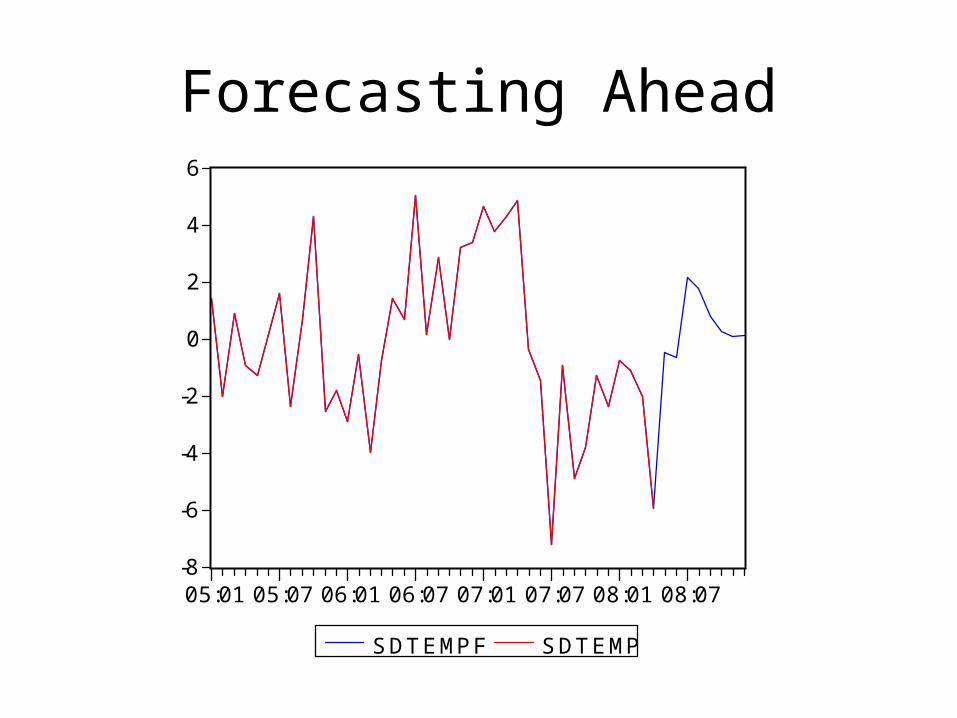
Forecasting Ahead

-8

-6

-4

-2

0

2

4

6

05:01 05:07 06:01 06:07 07:01 07:07 08:01 08:07

SDT EMPF SDT EMP

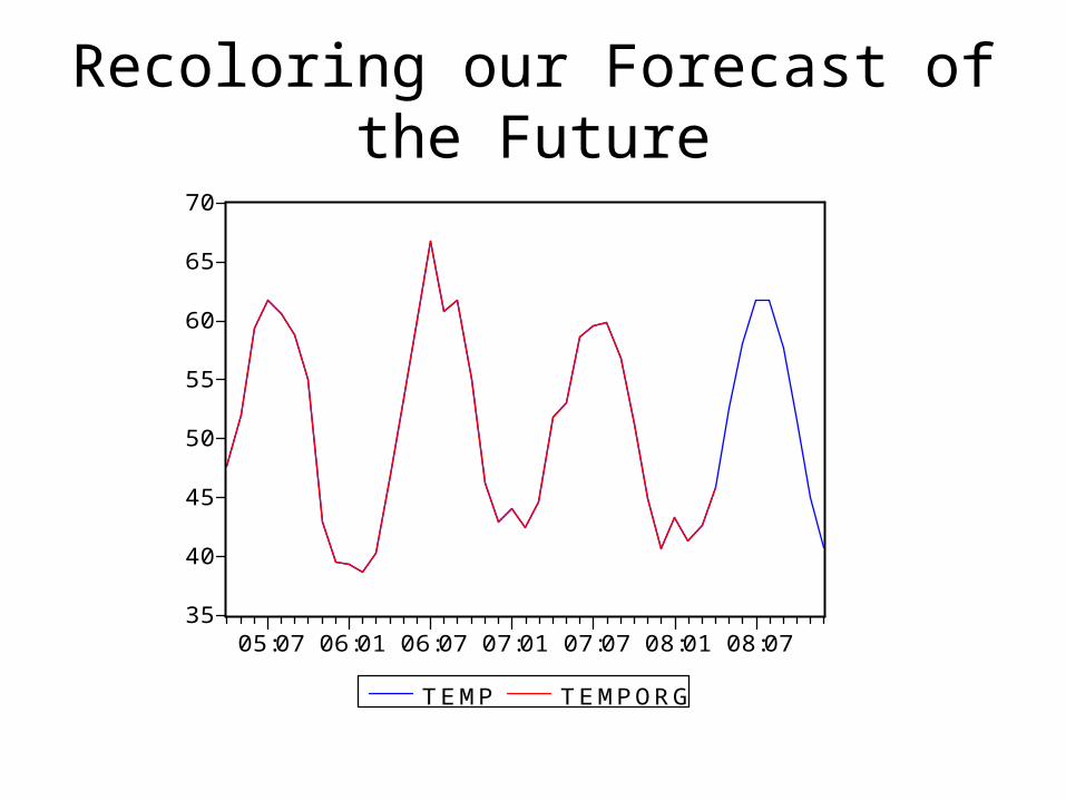
Recoloring our Forecast of the Future

35

40

45

50

55

60

65

70

05:07 06:01 06:07 07:01 07:07 08:01 08:07

T EMP T EMPORG

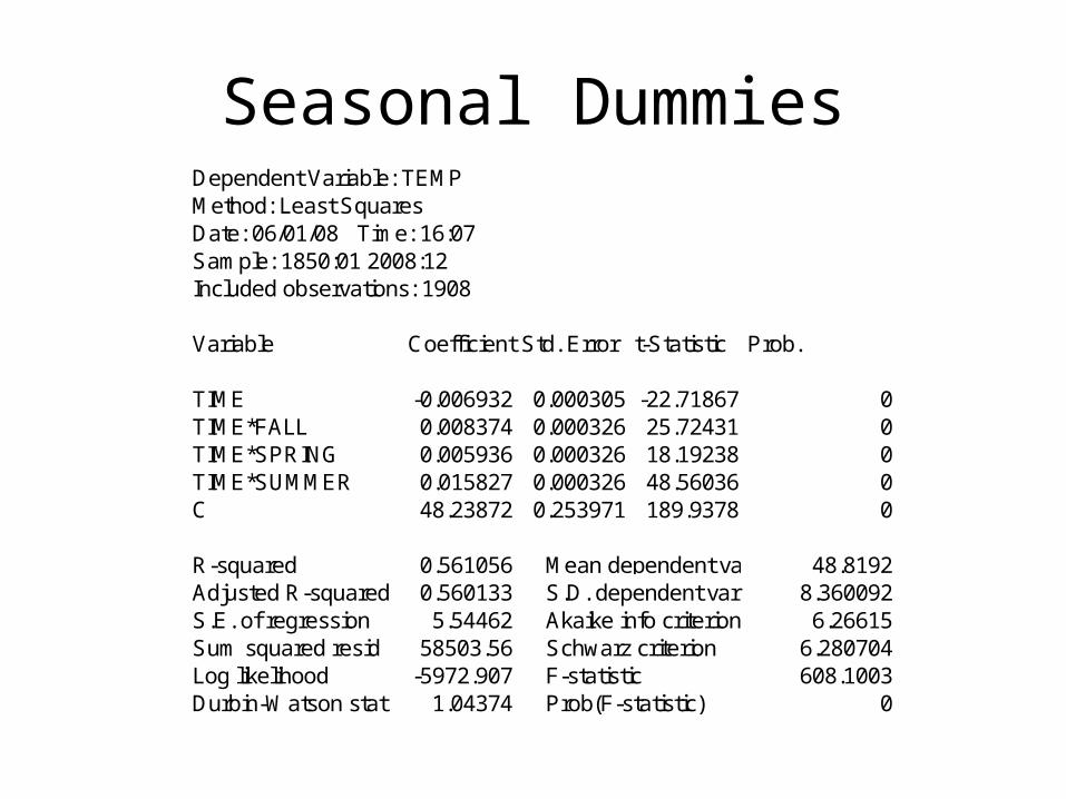
Seasonal DummiesDependent Variable: TEMPMethod: Least SquaresDate: 06/01/08 Time: 16:07Sample: 1850:01 2008:12Included observations: 1908

Variable Coefficient Std. Error t-Statistic Prob.

TIME -0.006932 0.000305 -22.71867 0TIME*FALL 0.008374 0.000326 25.72431 0TIME*SPRING 0.005936 0.000326 18.19238 0TIME*SUMMER 0.015827 0.000326 48.56036 0C 48.23872 0.253971 189.9378 0

R-squared 0.561056 Mean dependent var 48.8192Adjusted R-squared 0.560133 S.D. dependent var 8.360092S.E. of regression 5.54462 Akaike info criterion 6.26615Sum squared resid 58503.56 Schwarz criterion 6.280704Log likelihood -5972.907 F-statistic 608.1003Durbin-Watson stat 1.04374 Prob(F-statistic) 0

Conclusion

We must look to other data such as rainfall, sea levels, ocean

temperatures, C02 data to say that global warming does exist.