Transportation Statistics Annual Report 1999 - gouv · Bingsong Fang John Fuller Robert Gibson Lee...
187
Transcript of Transportation Statistics Annual Report 1999 - gouv · Bingsong Fang John Fuller Robert Gibson Lee...


Transportation Statistics Annual Report
1999
Bureau of Transportation
Statistics
BTS99-03 U.S. Department of Transportation

All material contained in this report is in the public domain andmay be used and reprinted without special permission; citationas to source is required.
Recommended citationU.S. Department of TransportationBureau of Transportation StatisticsTransportation Statistics Annual Report 1999BTS99-03Washington, DC: 1999
To obtain copies of this report and other BTS products contact:Customer ServiceBureau of Transportation StatisticsU.S. Department of Transportation400 7th Street SW, Room 3430Washington, DC 20590
phone 202.366.DATAfax 202.366.3640email (product orders) [email protected] by phone 800.853.1351statistics by email [email protected] www.bts.gov
PhotographsSummary: Lock & Dam 14, Le Claire, IA, by C. Arney for theU.S. Army Corps of Engineers.
Ch. 1: Alaska Oil Pipeline by B. Heims for the U.S. Army Corpsof Engineers.
Ch. 2, 3, & 6: Gate Information and Luggage at Reagan NationalAirport, Washington, DC, and MARC train in Baltimore City,MD, by M. Fenn for the Bureau of Transportation Statistics.
Ch. 4: Maine Avenue Waterfront, Washington, DC, by S. Gieseckefor the Bureau of Transportation Statistics.
Ch. 5: Dredging, New York District, U.S. Army Corps ofEngineers.

U.S. Department of Transportation
Rodney E. SlaterSecretary
Mortimer L. DowneyDeputy Secretary
Bureau of Transportation Statistics
Ashish K. SenDirector
Richard R. KowalewskiDeputy Director
Rolf R. SchmittAssociate Director forTransportation Studies
Susan J. LaphamActing Associate Directorfor Statistical Programs andServices
Project ManagerWendell Fletcher
Assistant Project ManagerJoanne Sedor
EditorMarsha Fenn
Major ContributorsFelix Ammah-TagoeAudrey BuyrnJohn CikotaAlan CraneBingsong FangJohn FullerRobert GibsonLee GiesbrechtDavid GreeneXiaoli HanPeter KuhnAnna Lynn LaCombe
Susan LaphamWilliam MallettPeter MontagueAlexander NewcomerKirsten OldenburgJoel PalleyLisa RandallMichael RossettiMark SaffordPaul SchimekRolf SchmittBasav Sen
Acknowledgments
Cover DesignOmniDigital, Inc.Ginny McDonagh
Report Layout andProductionOmniDigital, Inc.Gardner SmithLinda Rolla
Other ContributorsCarol BrandtEugene BrownRussell CapelleLillian ChapmanStacy DavisSelena GieseckeEmilia GovanMadeline GrossThomas HoffmanGary KraussMichael MyersAlan PisarskiTonia RifaeySimon RandrianariveloBruce Spear

Table of Contents � v
PREFACE . . . . . . . . . . . . . . . . . . . . . . . . . . . . . . . . . . . . . . . . . . . . . . . . . . . . . . . . . . . . . ix
SUMMARY . . . . . . . . . . . . . . . . . . . . . . . . . . . . . . . . . . . . . . . . . . . . . . . . . . . . . . . . . . . . 1
1 SYSTEM EXTENT AND CONDITION . . . . . . . . . . . . . . . . . . . . . . . . . . . . . . . . . . . . . 13Highway . . . . . . . . . . . . . . . . . . . . . . . . . . . . . . . . . . . . . . . . . . . . . . . . . . . . . . . . . . . . . . 14Rail . . . . . . . . . . . . . . . . . . . . . . . . . . . . . . . . . . . . . . . . . . . . . . . . . . . . . . . . . . . . . . . . . 21Air . . . . . . . . . . . . . . . . . . . . . . . . . . . . . . . . . . . . . . . . . . . . . . . . . . . . . . . . . . . . . . . . . . 22Water . . . . . . . . . . . . . . . . . . . . . . . . . . . . . . . . . . . . . . . . . . . . . . . . . . . . . . . . . . . . . . . . 25Oil and Gas Pipelines . . . . . . . . . . . . . . . . . . . . . . . . . . . . . . . . . . . . . . . . . . . . . . . . . . . . 27Transit . . . . . . . . . . . . . . . . . . . . . . . . . . . . . . . . . . . . . . . . . . . . . . . . . . . . . . . . . . . . . . . 29Information Technology Use in Transportation . . . . . . . . . . . . . . . . . . . . . . . . . . . . . . . . . 31Data Needs . . . . . . . . . . . . . . . . . . . . . . . . . . . . . . . . . . . . . . . . . . . . . . . . . . . . . . . . . . . . 32References . . . . . . . . . . . . . . . . . . . . . . . . . . . . . . . . . . . . . . . . . . . . . . . . . . . . . . . . . . . . . 34Boxes1-1 High-Speed Rail Corridor Status . . . . . . . . . . . . . . . . . . . . . . . . . . . . . . . . . . . . . . . . 231-2 Report on Maritime Trade and Water Transportation . . . . . . . . . . . . . . . . . . . . . . . . 281-3 Railroad Applications for Information Technology . . . . . . . . . . . . . . . . . . . . . . . . . . . 32
2 TRANSPORTATION SYSTEM USE AND PERFORMANCE . . . . . . . . . . . . . . . . . . . . . 35Passenger Travel . . . . . . . . . . . . . . . . . . . . . . . . . . . . . . . . . . . . . . . . . . . . . . . . . . . . . . . . 35Domestic Freight . . . . . . . . . . . . . . . . . . . . . . . . . . . . . . . . . . . . . . . . . . . . . . . . . . . . . . . . 42International Freight . . . . . . . . . . . . . . . . . . . . . . . . . . . . . . . . . . . . . . . . . . . . . . . . . . . . . 48Use and Performance . . . . . . . . . . . . . . . . . . . . . . . . . . . . . . . . . . . . . . . . . . . . . . . . . . . . 53References . . . . . . . . . . . . . . . . . . . . . . . . . . . . . . . . . . . . . . . . . . . . . . . . . . . . . . . . . . . . . 65Boxes2-1 The Commodity Flow Survey and Supplementary Freight Data . . . . . . . . . . . . . . . . . 43
3 TRANSPORTATION AND THE ECONOMY . . . . . . . . . . . . . . . . . . . . . . . . . . . . . . . . 67Transportation and Gross Domestic Product . . . . . . . . . . . . . . . . . . . . . . . . . . . . . . . . . . . 67Public Transportation Revenues and Expenditures . . . . . . . . . . . . . . . . . . . . . . . . . . . . . . . 78Capital Investment and Capital Stock . . . . . . . . . . . . . . . . . . . . . . . . . . . . . . . . . . . . . . . . 80Data Needs . . . . . . . . . . . . . . . . . . . . . . . . . . . . . . . . . . . . . . . . . . . . . . . . . . . . . . . . . . . . 81References . . . . . . . . . . . . . . . . . . . . . . . . . . . . . . . . . . . . . . . . . . . . . . . . . . . . . . . . . . . . . 82
4 TRANSPORTATION SAFETY . . . . . . . . . . . . . . . . . . . . . . . . . . . . . . . . . . . . . . . . . . . . 83Long-Term Trends . . . . . . . . . . . . . . . . . . . . . . . . . . . . . . . . . . . . . . . . . . . . . . . . . . . . . . 84Transportation of School Children . . . . . . . . . . . . . . . . . . . . . . . . . . . . . . . . . . . . . . . . . . 88Pedestrian and Bicycle Safety . . . . . . . . . . . . . . . . . . . . . . . . . . . . . . . . . . . . . . . . . . . . . . . 93Terrorism and Transportation Security . . . . . . . . . . . . . . . . . . . . . . . . . . . . . . . . . . . . . . . 96International Trends in Road Safety . . . . . . . . . . . . . . . . . . . . . . . . . . . . . . . . . . . . . . . . . 98Data Needs . . . . . . . . . . . . . . . . . . . . . . . . . . . . . . . . . . . . . . . . . . . . . . . . . . . . . . . . . . . 100References . . . . . . . . . . . . . . . . . . . . . . . . . . . . . . . . . . . . . . . . . . . . . . . . . . . . . . . . . . . . 101Boxes4-1 Occupant Protection . . . . . . . . . . . . . . . . . . . . . . . . . . . . . . . . . . . . . . . . . . . . . . . . . 90
Table of Contents

vi � Transportation Statistics Annual Report 1999
5 TRANSPORTATION, ENERGY, AND THE ENVIRONMENT . . . . . . . . . . . . . . . . . . 103Energy . . . . . . . . . . . . . . . . . . . . . . . . . . . . . . . . . . . . . . . . . . . . . . . . . . . . . . . . . . . . . . 104Greenhouse Gases . . . . . . . . . . . . . . . . . . . . . . . . . . . . . . . . . . . . . . . . . . . . . . . . . . . . . . 114Environment . . . . . . . . . . . . . . . . . . . . . . . . . . . . . . . . . . . . . . . . . . . . . . . . . . . . . . . . . . 116Data Needs . . . . . . . . . . . . . . . . . . . . . . . . . . . . . . . . . . . . . . . . . . . . . . . . . . . . . . . . . . . 135References . . . . . . . . . . . . . . . . . . . . . . . . . . . . . . . . . . . . . . . . . . . . . . . . . . . . . . . . . . . . 139
6 THE STATE OF TRANSPORTATION STATISTICS . . . . . . . . . . . . . . . . . . . . . . . . . . . 143References . . . . . . . . . . . . . . . . . . . . . . . . . . . . . . . . . . . . . . . . . . . . . . . . . . . . . . . . . . . . 149Boxes6-1 Domestic Transportation of International Trade . . . . . . . . . . . . . . . . . . . . . . . . . . . . 147
LIST OF ACRONYMS . . . . . . . . . . . . . . . . . . . . . . . . . . . . . . . . . . . . . . . . . . . . . . . . . 151
U.S./METRIC CONVERSIONS AND ENERGY UNIT EQUIVALENTS . . . . . . . . . . . . 155
INDEX . . . . . . . . . . . . . . . . . . . . . . . . . . . . . . . . . . . . . . . . . . . . . . . . . . . . . . . . . . . . . . 157
List of Tables1 SYSTEM EXTENT AND CONDITION
1-1 Major Elements of the Transportation System: 1997 . . . . . . . . . . . . . . . . . . . . . . . . 151-2 Highway Pavement Conditions: 1994–97 . . . . . . . . . . . . . . . . . . . . . . . . . . . . . . . . 181-3 Highway Bridge Conditions: 1990 and 1997 . . . . . . . . . . . . . . . . . . . . . . . . . . . . . 201-4 U.S.-Flag Waterborne Cargo-Carrying Vessel Fleet Profile: 1997 . . . . . . . . . . . . . . .27
2 TRANSPORTATION SYSTEM USE AND PERFORMANCE2-1 Population and Passenger Travel in the United States: 1977 and 1995 . . . . . . . . . . 362-2 Daily and Long-Distance Trips by Mode: 1995 . . . . . . . . . . . . . . . . . . . . . . . . . . . 372-3 Person Trips per Day by Purpose and Sex: 1995 . . . . . . . . . . . . . . . . . . . . . . . . . . . 402-4 Domestic- and Export-Bound Freight Shipments within the
United States: 1993 and 1997 . . . . . . . . . . . . . . . . . . . . . . . . . . . . . . . . . . . . . . . . . 442-5 Modal Shares of Freight Shipments within the United States
by Domestic Establishments: 1993 and 1997 . . . . . . . . . . . . . . . . . . . . . . . . . . . . . 462-6 U.S. Freight Shipments by Distance Shipped: 1993 and 1997 . . . . . . . . . . . . . . . . . 472-7 Major Commodities Shipped in the United States: 1997 . . . . . . . . . . . . . . . . . . . . . 472-8 Shipments by Size: 1993 and 1997 . . . . . . . . . . . . . . . . . . . . . . . . . . . . . . . . . . . . . 492-9 Top 10 U.S. Merchandise Trade Partners by Value:
1980 and 1997 . . . . . . . . . . . . . . . . . . . . . . . . . . . . . . . . . . . . . . . . . . . . . . . . . . . 492-10 Top Water Ports for International Trade: 1997 . . . . . . . . . . . . . . . . . . . . . . . . . . . . 522-11 Highway Vehicle-Miles Traveled by Functional Class: 1980–97 . . . . . . . . . . . . . . . 562-12 Urban Congestion Indicators for 70 Urban Areas: Selected Years . . . . . . . . . . . . . . 572-13 Urban Transit Indicators: 1987–97 . . . . . . . . . . . . . . . . . . . . . . . . . . . . . . . . . . . . . 622-14 Top 10 State Rail Freight Flows and Major Commodities: 1997 . . . . . . . . . . . . . . 64
List of Tables � vii
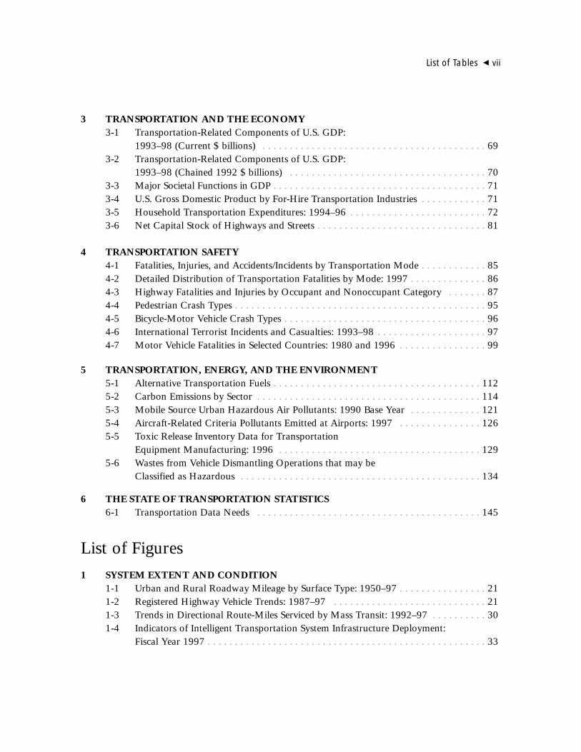
3 TRANSPORTATION AND THE ECONOMY3-1 Transportation-Related Components of U.S. GDP:
1993–98 (Current $ billions) . . . . . . . . . . . . . . . . . . . . . . . . . . . . . . . . . . . . . . . . . 693-2 Transportation-Related Components of U.S. GDP:
1993–98 (Chained 1992 $ billions) . . . . . . . . . . . . . . . . . . . . . . . . . . . . . . . . . . . . 703-3 Major Societal Functions in GDP . . . . . . . . . . . . . . . . . . . . . . . . . . . . . . . . . . . . . . . 713-4 U.S. Gross Domestic Product by For-Hire Transportation Industries . . . . . . . . . . . . 713-5 Household Transportation Expenditures: 1994–96 . . . . . . . . . . . . . . . . . . . . . . . . . 723-6 Net Capital Stock of Highways and Streets . . . . . . . . . . . . . . . . . . . . . . . . . . . . . . . 81
4 TRANSPORTATION SAFETY4-1 Fatalities, Injuries, and Accidents/Incidents by Transportation Mode . . . . . . . . . . . . 854-2 Detailed Distribution of Transportation Fatalities by Mode: 1997 . . . . . . . . . . . . . . 864-3 Highway Fatalities and Injuries by Occupant and Nonoccupant Category . . . . . . . 874-4 Pedestrian Crash Types . . . . . . . . . . . . . . . . . . . . . . . . . . . . . . . . . . . . . . . . . . . . . . 954-5 Bicycle-Motor Vehicle Crash Types . . . . . . . . . . . . . . . . . . . . . . . . . . . . . . . . . . . . . 964-6 International Terrorist Incidents and Casualties: 1993–98 . . . . . . . . . . . . . . . . . . . . 974-7 Motor Vehicle Fatalities in Selected Countries: 1980 and 1996 . . . . . . . . . . . . . . . . 99
5 TRANSPORTATION, ENERGY, AND THE ENVIRONMENT5-1 Alternative Transportation Fuels . . . . . . . . . . . . . . . . . . . . . . . . . . . . . . . . . . . . . . 1125-2 Carbon Emissions by Sector . . . . . . . . . . . . . . . . . . . . . . . . . . . . . . . . . . . . . . . . . 1145-3 Mobile Source Urban Hazardous Air Pollutants: 1990 Base Year . . . . . . . . . . . . . 1215-4 Aircraft-Related Criteria Pollutants Emitted at Airports: 1997 . . . . . . . . . . . . . . . 1265-5 Toxic Release Inventory Data for Transportation
Equipment Manufacturing: 1996 . . . . . . . . . . . . . . . . . . . . . . . . . . . . . . . . . . . . . 1295-6 Wastes from Vehicle Dismantling Operations that may be
Classified as Hazardous . . . . . . . . . . . . . . . . . . . . . . . . . . . . . . . . . . . . . . . . . . . . 134
6 THE STATE OF TRANSPORTATION STATISTICS6-1 Transportation Data Needs . . . . . . . . . . . . . . . . . . . . . . . . . . . . . . . . . . . . . . . . . 145
List of Figures1 SYSTEM EXTENT AND CONDITION
1-1 Urban and Rural Roadway Mileage by Surface Type: 1950–97 . . . . . . . . . . . . . . . . 211-2 Registered Highway Vehicle Trends: 1987–97 . . . . . . . . . . . . . . . . . . . . . . . . . . . . 211-3 Trends in Directional Route-Miles Serviced by Mass Transit: 1992–97 . . . . . . . . . . 301-4 Indicators of Intelligent Transportation System Infrastructure Deployment:
Fiscal Year 1997 . . . . . . . . . . . . . . . . . . . . . . . . . . . . . . . . . . . . . . . . . . . . . . . . . . . 33

viii � Transportation Statistics Annual Report 1999
2 TRANSPORTATION SYSTEM USE AND PERFORMANCE2-1 Person-Miles Traveled per Day: 1995 . . . . . . . . . . . . . . . . . . . . . . . . . . . . . . . . . . . 392-2 Long-Distance Trips per Person: 1995 . . . . . . . . . . . . . . . . . . . . . . . . . . . . . . . . . . 402-3 Freight Shipments and Related Factors of Growth: 1993–97 . . . . . . . . . . . . . . . . . . 452-4 Modal Shares of U.S. Merchandise Trade by Value and Tons: 1997 . . . . . . . . . . . . 512-5 Top Border Land Ports: 1997 . . . . . . . . . . . . . . . . . . . . . . . . . . . . . . . . . . . . . . . . . 542-6 Top Freight Gateways by Shipment Value: 1997 . . . . . . . . . . . . . . . . . . . . . . . . . . . 552-7 Congested Person-Miles of Travel in 70 Urban Areas . . . . . . . . . . . . . . . . . . . . . . . 562-8 Enplanements at Major Hubs: 1987 and 1997 . . . . . . . . . . . . . . . . . . . . . . . . . . . . 582-9 Tonnage Handled by Major Ports: 1997 . . . . . . . . . . . . . . . . . . . . . . . . . . . . . . . . . 602-10 Largest Transit Markets: 1997 . . . . . . . . . . . . . . . . . . . . . . . . . . . . . . . . . . . . . . . . 612-11 ADA-Accessible Vehicles by Mode: 1994–97 . . . . . . . . . . . . . . . . . . . . . . . . . . . . . 632-12 Railroad Network Showing Volume of Freight: 1997 . . . . . . . . . . . . . . . . . . . . . . . 632-13 Rail Carload Mix: 1997 . . . . . . . . . . . . . . . . . . . . . . . . . . . . . . . . . . . . . . . . . . . . . 64
3 TRANSPORTATION AND THE ECONOMY3-1 Characteristics of Household Transportation Expenditures by Age Group . . . . . . . 733-2 Modal Share of Transportation Industry Employment: 1997 . . . . . . . . . . . . . . . . . 733-3 Employment in Transportation Occupations: 1997 . . . . . . . . . . . . . . . . . . . . . . . . . 753-4 Labor Productivity Trends by Mode . . . . . . . . . . . . . . . . . . . . . . . . . . . . . . . . . . . . 773-5 Growth in Government Transportation Revenues: 1986–95 . . . . . . . . . . . . . . . . . . 793-6 Government Transportation Revenues by Mode: Fiscal Year 1995 . . . . . . . . . . . . . 793-7 Growth in Government Transportation Expenditures: 1986–95 . . . . . . . . . . . . . . . 79
4 TRANSPORTATION SAFETY4-1 Fatality Rates for Selected Modes . . . . . . . . . . . . . . . . . . . . . . . . . . . . . . . . . . . . . . 894-2 School Transportation by Mode: 1995 . . . . . . . . . . . . . . . . . . . . . . . . . . . . . . . . . . 914-3 Fatal Crashes and Occupant Fatalities Among School-Age
Children by Vehicle Type: 1997 . . . . . . . . . . . . . . . . . . . . . . . . . . . . . . . . . . . . . . . 914-4 Relative Change in Motorist, Bicyclist, and Pedestrian Fatalities: 1975–97 . . . . . . . . . 944-5 Bicycle Fatalities by Age of Bicyclist: 1975–97 . . . . . . . . . . . . . . . . . . . . . . . . . . . . 954-6 World Motor Vehicle Registration Trends: 1960–95 . . . . . . . . . . . . . . . . . . . . . . . . 98
5 TRANSPORTATION, ENERGY, AND THE ENVIRONMENT5-1 Transportation Energy and Economic Activity: 1960–97 . . . . . . . . . . . . . . . . . . . 1055-2 Transportation Energy Use by Mode: 1997 . . . . . . . . . . . . . . . . . . . . . . . . . . . . . 1055-3 Highway Vehicle Average Fuel Consumption: 1960–97 . . . . . . . . . . . . . . . . . . . . 1065-4 U.S. Sales of Domestic and Foreign Light-Duty Vehicles by Class . . . . . . . . . . . . . 1085-5 Fuel Economy of Light Vehicles by Class and Sales Change: 1990–97 . . . . . . . . . . 1095-6 Petroleum Production and Imports: 1980–98 . . . . . . . . . . . . . . . . . . . . . . . . . . . . 1105-7 World Oil Price: 1980–98 . . . . . . . . . . . . . . . . . . . . . . . . . . . . . . . . . . . . . . . . . . . 1115-8 National Transportation Emissions Trends Index: 1970–97 . . . . . . . . . . . . . . . . . 1185-9 Modal Shares of Key Criteria Pollutants from Transportation Sources: 1997 . . . . 1195-10 National Air Quality Trends Index for Criteria Pollutants: 1975–97 . . . . . . . . . . . 120
Congress requires the Bureau of Transportation Statistics to transmit an
annual report on transportation statistics to the President and Congress.
Transportation Statistics Annual Report 1999 is the sixth such report
prepared in response to this congressional mandate, laid out in 49 U.S.C. 111 (j).
The report discusses the extent and condition of the transportation system; its use,
performance, and safety record; transportation’s economic contributions and costs;
and its energy and environmental impacts. All modes of transportation are covered
in the report.
Special features this year include an update of the status of high-speed rail
corridors and pedestrian and bicycle safety. In addition, the environmental impacts
discussion has been expanded to include transportation infrastructure, equipment
manufacturing, vehicle maintenance and disposal, and vehicle emissions.
Preface
�
ix

The Bureau of Transportation Statistics (BTS) presents the sixthTransportation Statistics Annual Report. Mandated by Congress, the reportdiscusses the U.S. transportation system, including its physical components,
economic performance, safety record, and related energy and environmentalimpacts. It also assesses the state of transportation statistics.
EXTENT AND CONDITION OF THE U.S.TRANSPORTATION SYSTEM
The nation’s inventory of transportation infrastructure and vehicles shows a contin-uing trend of expansion and improvement, although a few exceptions exist. From1987 to 1997, public road mileage increased by less than 2 percent, and the per-centage of paved roadway increased from 56 percent to 61 percent. Surface rough-ness measurements indicate that the conditions of most roadways are improving.Likewise, the percentage of bridges classified as functionally and/or structurallyobsolete decreased noticeably since 1990, dropping from 41 percent to 30 percent.
The nation’s highway vehicle fleet consisted of about 212 million vehicles in 1997,nearly 28 million more vehicles than a decade earlier. Of special note has been thedramatic growth in the number of sport utility vehicles and other light trucks. Thissegment of the fleet increased from 41 million vehicles in 1987 to over 70 million in
�
1
Summary

1997, accounting for 33 percent of the fleet. Still,passenger cars accounted for over 61 percent ofthe total highway fleet (nearly 130 million vehi-cles), despite a 5 million vehicle decrease in thenumber of automobiles over the past decade.Large trucks and buses show a more moderateincrease.
In 1997, there were 9 Class I freight railroads(railroads with at least $256 million in operatingrevenues) in the United States, 34 regional rail-roads, and 507 local railroads. The railroadindustry operated over 170,000 miles of track,over 70 percent of which was operated by ClassI railroads. Since 1980, Class I traffic, measuredin ton-miles, increased by 47 percent, while milesof road owned declined by 38 percent due to thesale of track to smaller railroads and abandon-ment. In the case of passenger rail, the NationalRailroad Passenger Corporation, better knownas Amtrak, operated more than 250 intercitytrains per day, along a 22,000 mile network in44 states with service to 500 communities in fis-cal year (FY) 1998.
In 1997, the United States had 18,345 air-ports, a 20 percent increase compared with1980. The increase was due to the addition ofmore than 3,200 general aviation airports. Thenumber of airports served by certificated aircraftdecreased from 730 to 660. The condition ofrunway surfaces improved overall, especially atairports not regularly served by commercial car-riers. (Runway surface conditions at commercialcarrier airports were generally in better condi-tion than those at airports not served by com-mercial carriers.)
The number of certificated aircraft in opera-tion grew steadily, increasing to more than 7,600in 1997 (excluding air taxi aircraft operated innonscheduled service). This represents a 4 per-cent increase over 1992, which is the first yearfor which a comprehensive commercial aircraftinventory is available. More than 190,000 gen-
eral aviation aircraft were reported active in1997, 60 percent of which were flown primarilyfor personal use. In 1997, there were 91 air car-riers (both passenger and freight) operating inthe United States.
The number of both commercial and recre-ational boats continued to increase in 1997. TheU.S.-flag commercial vessel fleet was over41,400 in 1997 compared with 38,800 in 1980.Approximately 12.3 million recreational boatswere registered in the United States in 1997 com-pared with 10 million in 1987, representing a 23percent increase in registered recreational water-craft during that decade.
In 1997, the nation’s waterborne commercewas handled by 3,726 public marine terminals.These terminals were about equally dividedamong deep-draft (ocean and Great Lake) andshallow-draft (inland waterway) facilities. Mostinland facilities (86 percent) were used for trans-porting bulk commodities, while coastal facilitieswere more evenly divided between bulk com-modities and general cargo—about 41 percentand 38 percent, respectively.
Over the next few years, coastal ports mayface the challenge of handling the next genera-tion of containerships that have the capacity of4,500 20-foot equivalent container units (TEUs)or more and drafts of 40 to 46 feet when fullyloaded. Only 5 of the top 15 U.S. containerports—Baltimore, Tacoma, Hampton Roads,Long Beach, and Seattle—currently have ade-quate channel depths, and only those on the westcoast have adequate berth depths to accommo-date these vessels. In addition, ports may need toexpand terminal infrastructure and improve railand highway connections to facilitate theincreased volumes of cargo from these ships.Many ports have already initiated expansionprojects to accommodate these ships. How effec-tively U.S. ports handle this next generation ofcontainerships will have implications for the effi-
2 � Transportation Statistics Annual Report 1999
ciency of the U.S. transportation system and U.S.trade competitiveness.
Oil and gas pipeline mileage remained rela-tively constant in the 1990s. Because comprehen-sive oil and gas pipeline data are not available, anaccurate assessment of total mileage does not cur-rently exist. Current efforts to develop geograph-ic information systems on liquid and natural gasnetworks may narrow this data gap.
In 1997, there were 556 federally assisted tran-sit agencies urbanized areas, operating more than76,000 vehicles and providing 8 billion passengertrips. Most transit trips and passenger-miles are onbuses and demand responsive vehicles, whichaccount for three-quarters of all transit vehicles.Federally assisted mass transit infrastructureincreased modestly during the 1992 to 1997 peri-od. Increases in new fixed-guideway mileage (bothrail and nonrail) are evident. In particular, exclu-sive and access-controlled bus lanes covered 60percent more route-miles in 1997 than in 1992.Fixed-guideway mileage increased by 21 percentfrom 1992 to 1997, reaching 10,800 directionalroute-miles. Directional route mileage for busesoperating on mixed rights-of-way, however, fluc-tuated from year to year between 1992 and 1997,with no evident pattern of growth or decline.
The mass transit vehicle fleet grew between1992 and 1997, primarily due to increases invehicles used in demand responsive service andvanpools. Over three-quarters of vehicles operat-ed by federally assisted transit agencies providedservice in large urban areas with populations inexcess of 1 million people. Buses and demandresponsive vehicles accounted for the majority ofthe fleet—57 percent and 18 percent, respective-ly—and were more widely used than commuter,light, and heavy rail modes.
Nonfederally assisted transit agencies alsoprovide important services, especially in ruralareas. However, information about these ser-vices is limited.
Information technologies have long been animportant element in the transportation system,especially in the railroad, aviation, and marinemodes. In recent years, technological advanceshave expanded information technology use in allmodes, including highways, transit, recreationalboating, and general aviation. The use of intelli-gent transportation systems (ITS) increased pri-marily in congested urban areas. A survey of thenation’s top 78 urban areas provides baselinedata on highway- and transit-related ITS imple-mentation which, when new survey data areobtained, may permit comparison of ITSchanges over time. Other advanced technologiessuch as Global Positioning Systems are alsobecoming an integral part of the transportationsystem, being used in air, marine, and land-basedtransportation modes.
TRANSPORTATION SYSTEM USEAND PERFORMANCE
Both freight transportation and passenger travelhave grown considerably in recent years. TheCommodity Flow Survey (CFS), undertaken byBTS and the Census Bureau, presents the broad-est picture of domestic commodity flows.According to preliminary CFS data and addi-tional estimates by BTS, between 1993 and1997, freight shipments increased about 17 per-cent by value, 14 percent by tons, and 10 percentby ton-miles. Preliminary BTS estimates alsoshow that nearly 14 billion tons of goods andraw materials, valued at over $8 trillion, movedover the U.S. transportation system in 1997, gen-erating nearly 4 trillion ton-miles. These figurestranslate into 38 million tons of commoditiesshipped on the nation’s transportation system ona typical day in 1997.
Most modes showed an increase in ton-miles.Shipments by air (including those involving truckand air) grew 86 percent in ton-miles, followed by
Summary � 3

parcel, postal, and courier services (41 percent),and truck (26 percent). Rail ton-miles (includingtruck and rail) increased by only 7 percent, whileton-miles by water decreased by about 3 percent.Nevertheless, trucking (including for-hire and pri-vate, and excluding parcel, postal, and courier ser-vices) was the mode used most frequently to movethe nation’s freight whether measured by value,tons, or ton-miles. Truck shipments accounted for69 percent of the total value of shipments in 1997about the same as in 1993. Trucking was followedby parcel, postal, and courier services; rail;pipeline; and air (including truck and air) in 1997.
Although many factors have affected thegrowth in U.S. freight shipments since 1993, sus-tained economic growth has been key. Economicgrowth has been accompanied by expansion ofinternational trade and increases in disposablepersonal income per capita. Other factors, suchas changes in how and where goods are pro-duced, have also contributed to the rise in freighttons and ton-miles over the past few years.
International trade has become an even moreintegral part of the U.S. economy, as illustratedby the increased value of U.S. merchandise trade.Between 1980 and 1997, the real dollar value ofU.S. merchandise trade more than tripled from$496 billion to $1.7 trillion (in chained 1992dollars). In addition, the ratio of the value of U.S.merchandise trade relative to U.S. GrossDomestic Product (GDP) doubled from about 11percent in 1980 to 23 percent in 1997. The traderelationship with Canada and Mexico has deep-ened over this period. In 1997, Canada andMexico together accounted for 30 percent of allU.S. trade by value, up from 22 percent in 1980.Trade with Asian Pacific countries also grew inimportance, so much so that in 1997, 5 Asiancountries were among the top 10 U.S. tradingpartners.
In U.S. international trade, water was the pre-dominant mode in terms of value and tonnage.In 1997, for example, waterborne trade account-ed for more than three-quarters of the tonnageand 40 percent of the value of U.S. internationaltrade. However, its share of the value of U.S.international trade declined from 62 percent in1980. Because of the rise of trade with AsianPacific countries a relative shift has occurred infreight handling from east coast to west coastports. Since 1988, foreign trade tonnage movedby water increased by 25 percent while domesticfreight tonnage moved by water remained aboutthe same—1.1 billion tons.
Between 1980 and 1997, air freight’s share ofthe value of U.S. international merchandise tradeincreased from 16 percent to nearly 28 percent.Commodities that move by air tend to be high invalue; air’s share of U.S. international trade byweight was less than 1 percent in 1997.
Passenger travel has grown rapidly in recentdecades. In 1995, people averaged about 4.3one-way trips per day and about 14,100 miles(39 miles per day) per year, up from 2.9 trips and9,500 miles (26 miles per day) in 1977. Long-distance travel (trips 100 miles or more fromhome) also increased over this period from 2.5roundtrips in 1977 to 3.9 in 1995. Several fac-tors account for this increase in travel, includinggreater labor force participation, income, andvehicle availability, and reduced travel cost.
People travel primarily by personal-use vehicles(PUVs) for both local daily travel and more infre-quent long-distance travel. Cars and other PUVsaccounted for about 90 percent of local trips and80 percent of long-distance trips. Bicycling andwalking accounted for 6.5 percent of local tripsand transit about 4 percent of local trips. Air trans-portation was the second most popular means oflong-distance travel, accounting for 18 percent oftrips, with buses about 2 percent and passengertrains about 0.5 percent of intercity trips.
4 � Transportation Statistics Annual Report 1999

Vehicle-miles traveled (vmt) by cars, trucks,and buses on public roads increased 68 percentbetween 1980 and 1997, with urban vmt growthoutpacing rural vmt 83 percent to 49 percent.One result of this growth has been greater con-gestion in the nation’s urban areas. According tothe Texas Transportation Institute’s (TTI) mostrecent analysis of urban highway congestion in70 urban areas, the estimated level of congestiondeclined in only two—Phoenix and Houston—between 1982 and 1996. Congestion in mostother urban areas increased, dramatically insome instances. According to TTI, the number ofurban areas in the study experiencing unaccept-able congestion rose from 10 of the 70 in 1982to 39 in 1996, with the average roadway con-gestion index rising about 25 percent from 0.91to 1.14. An index of 1.00 or greater was selectedas the threshold for unacceptable congestion.
In the 1980s and 1990s, air travel also grewdramatically. Domestic and international passen-ger enplanements at U.S. airports increased from302 million in 1980 to 575 million in 1997. On-time performance decreased only slightly sincethe early 1990s. The percentage of passengersdenied boarding (i.e., “bumped” from flightsbecause seats were oversold by the airline) on the10 largest U.S. air carriers has risen appreciablysince 1993 from 683,000 (0.15 percent of board-ings) to 1.1 million passengers (0.21 percent ofboardings) in 1997. While the percentage of mis-handled baggage has declined steadily since1992, the total number of consumer complaintsagainst major air carriers received by the U.S.Department of Transportation (DOT) increasedin 1997 for the second year in a row after sever-al years of decline. In 1997, 86 out of every 1million persons enplaned on a major airline reg-istered a complaint with DOT, the highest ratesince 1993.
Transit ridership remained relatively constantbetween 1987 and 1997 with 7.85 millionunlinked trips in 1987 compared with 7.98 mil-lion in 1997, while miles traveled increased fromabout 36 billion to 40 billion. Riders on busesand heavy rail constitute the majority of transitusers, but ridership stagnated over this period,while the number of riders on other modes—especially demand responsive service, light rail,and ferries—increased markedly. Ridership oncommuter rail increased by a moderate amount.The performance and general quality of transitservice in the United States seems to be improv-ing, at least for federally subsidized transit,which accounts for approximately 90 to 95 per-cent of total transit passenger-miles.
While freight rail traffic increased, passengerrail traffic remained relatively constant. Therewere 20.2 million Amtrak passengers in FY1997, about the same as the number in FY 1987.
TRANSPORTATION ANDTHE ECONOMY
Measures of transportation’s importance in thegrowing U.S. economy include the level of trans-portation-related production and consumption ofgoods and services, household spending, wagesand salaries, and government revenues and expen-ditures.
In 1997, transportation-related goods and ser-vices contributed $905 billion, or about 11 per-cent, to U.S. GDP. This is the broadest measureof transportation’s contribution to GDP.Transportation continued to rank fourth, afterhousing, health care, and food, in terms of soci-etal demand for goods and services.
A narrower measure of transportation’s eco-nomic role is the value-added by transportationservices, both for-hire and in-house. This mea-sure includes only those services that move peo-
Summary � 5

ple and goods on the transportation system. In1997, the for-hire transportation industry,together with warehousing, contributed $255billion to the U.S. economy.
The contribution of transportation servicesconducted by nontransportation industries (in-house transportation) to GDP are calculatedusing the Transportation Satellite Accounts.According to a recent BTS report, Trans-portation Satellite Accounts: A New Way ofMeasuring Transportation Services in America,in-house transportation services contributed $121billion in 1992, the most recent year analyzed.
Household expenditures also indicate theimportance of transportation in the U.S. econo-my. In 1996, households spent, on average,$6,400 on transportation, which is about 17 per-cent of total expenditures. Vehicle purchases werethe largest component of these expenditures. In1996, southern and rural households spent morethan 50 percent of their transportation budgetson purchasing new and used vehicles—more thanother regions and urban households.
In terms of employment, the for-hire trans-portation industry’s share of total employmentchanged little from 1990 to 1997, hoveringaround 3 percent of the total U.S. civilian laborforce. The largest portion of for-hire transporta-tion industry employment in 1997 was in thetrucking and warehousing group (41 percent),but the group’s annual growth rate was not aslarge as that of other modes such as transit. Also,trucking and warehousing had the largest shareof the for-hire transportation industry’s totalwages and salaries in 1997, but the air trans-portation industry’s share increased more dra-matically. Similarly, truck drivers accounted forthe largest percentage of transportation occupa-tions in 1997 (67.8 percent), which was a slight-ly lower share than throughout the 1980s and1990s. Occupations in the air mode experiencedthe fastest growth (12.4 percent gain) in 1997.
Based on limited data on transportation occu-pational wages and salaries, airline pilots andnavigators were paid the most in 1997 (althoughearnings declined from the past year), while busand taxi drivers were paid the least.
Labor productivity—the relationship betweenton-miles or passenger-miles to number ofemployees or employee-hours—varied by trans-portation modes. In the railroad industry, laborproductivity (measured by an index of passenger-miles, freight ton-miles, revenue, and other fac-tors) went up between 1990 and 1996 by a totalof 44.5 percent, which was faster than the petro-leum pipeline industry (36.1 percent), the airtransportation industry (both passenger andfreight—19.5 percent), and the trucking industry(17.7 percent).
All levels of government benefit from revenuesreceived from transportation. Transportationrevenue growth fluctuated considerably over thepast decade, but increased in constant dollarsfrom $83.5 billion in FY 1994 to $86.7 billion inFY 1995. States generated nearly one-half of
6 � Transportation Statistics Annual Report 1999
Other, 32%Housing, 24%
Health, 14%
Food, 12%Transportation, 11%
Education,7%
Major Societal Functions inGross Domestic Product: 1997
SOURCE: See table 3-3 in chapter 3.
total government transportation revenues in1995, followed by the federal government (32percent) and local governments (20 percent).Highways generated $66.74 billion (current dol-lars) or 71 percent in 1995. Fuels taxes are animportant source of highway revenue, accountingfor 85.8 percent of the Highway Trust Fund and60 percent of state highway revenues in 1995.
Government also contributed to transporta-tion’s role in the economy through public expen-ditures, including capital investment. All levels ofgovernment spent a total of $129.3 billion (cur-rent dollars) on all modes of transportation in1995. State and local governments spent about69 percent of total government transportationexpenditures.
As in past years, more government funds werespent on highways than on all other transporta-tion modes combined. In 1995, highway spend-ing was $79.2 billion, about 61 percent of totalgovernment expenditures, while transit receivedabout 20 percent. State and local governmentscontinued to spend more on highways, transit,and pipelines, while the federal governmentspent more on air, water, and rail. In 1995, high-ways also continued to receive most (71 percent)of the $60.6 billion capital investment made bygovernments for infrastructure and equipment, asum that is nearly half of all government expen-ditures. In 1996, transportation infrastructurecapital stock in highways and streets was worth$1.3 trillion, nearly all owned by state and localgovernments.
TRANSPORTATION SAFETY
Thanks to technological innovations, education-al campaigns, and diligent enforcement efforts,the United States has made tremendous progressin transportation safety, especially in the lastthree decades. Despite all of these activities,work still remains. More than 44,000 people
died in transportation incidents during 1997,equivalent to the population of a large suburbantown. The number one goal of the Departmentof Transportation is to reduce this total in theyears ahead.
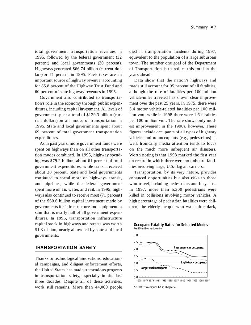
Data show that the nation’s highways androads still account for 95 percent of all fatalities,although the rate of fatalities per 100 millionvehicle-miles traveled has shown clear improve-ment over the past 25 years. In 1975, there were3.4 motor vehicle-related fatalities per 100 mil-lion vmt, while in 1998 there were 1.6 fatalitiesper 100 million vmt. The rate shows only mod-est improvement in the 1990s, however. Thesefigures include occupants of all types of highwayvehicles and nonoccupants (e.g., pedestrians) aswell. Ironically, media attention tends to focuson the much more infrequent air disasters.Worth noting is that 1998 marked the first yearon record in which there were no onboard fatal-ities involving large, U.S.-flag air carriers.
Transportation, by its very nature, providesenhanced opportunities but also risks to thosewho travel, including pedestrians and bicyclists.In 1997, more than 5,300 pedestrians werekilled in collisions involving motor vehicles. Ahigh percentage of pedestrian fatalities were chil-dren, the elderly, people who walk after dark,
Summary � 7
1975 1977
Passenger car occupants
1979 1981 1983 1985 1987 1989 1991 1993 1995 19970.0
0.5
1.0
1.5
2.0
2.5
3.0
Large-truck occupants
Light-truck occupants
Occupant Fatality Rates for Selected ModesPer 100 million vehicle-miles
SOURCE: See figure 4-1 in chapter 4.

and intoxicated individuals. In 1997, 814 bicy-clists or pedalcyclists died and 58,000 wereinjured in traffic crashes with motor vehicles.
Despite our growing knowledge about trans-portation safety, there are still many unmet dataneeds, such as risk exposure measures for waterand pipeline transportation. Even for highwayexposure, the accuracy of vmt is unclear. To gaina deeper understanding of safety, exposure mea-sures are needed for specific populations such asthe elderly, as well as for specific conditions suchas adverse weather.
Outcome data also need improvement.Statistics for fatalities, injuries, crashes, and prop-erty damages should be in a clear, easy-to-under-stand formats, distinguishing occupants fromnonoccupants, and transportation incidents fromnontransportation incidents. Ideally, all modeswould have reporting frameworks, including def-initions, measures, and explanatory text, thatenable quick comparisons across transportationtypes. With increasing international motorizationand globalization, the United States also needs towork with safety officials in other countries todevelop statistics that permit valid comparisonsacross countries. In this manner, a robust stock ofinformation about specific risk factors, causes,and societal impacts of transportation crashesand incidents can be built.
ENERGY
Petroleum provides about 97 percent of thetransportation sector’s energy requirements. Inrecent years, the abundance of petroleum sup-plies and low fuel prices has encouraged con-sumption and led to increased imports andgreater dependence on foreign oil. The volume ofimported oil exceeded domestic production in1997, the first time in U.S. history.
Highway vehicles accounted for about 80 per-cent of total transportation energy use in 1997.
Average fuel economy for the new passenger carfleet has ranged from 27.9 miles per gallon to28.8 miles per gallon since 1988. Efficiency gainshave been offset by the increases in the weightand power of passenger cars and shifts to lessfuel-efficient vehicles. In 1997, sales of mostlight-truck classes gained while most automobileclasses declined. Light trucks consume more fuelthan cars.
Although technologies are available for rais-ing vehicle efficiency further, there is little con-sumer demand or regulatory incentive for suchimprovement. Further, oil prices may remain lowfor a while, at least until Asian economies recov-er and their demand for oil increases. All thesefactors make it likely that petroleum consump-tion will continue to grow. While there is someinterest in alternative and replacement fuels andelectric vehicles that could reduce air emissionsand oil dependence, those options still involvemany uncertainties and limitations.
ENVIRONMENT
Serious environmental issues continue to be asso-ciated with transportation. The use of petroleumis responsible for most of the environmental prob-lems resulting from transportation, including car-bon dioxide emissions that may contribute toglobal climate change. In 1997, the transportationsector contributed about 26 percent of all U.S.emissions covered by an international agreement,the Kyoto Protocol. If Congress consents to theProtocol, the announced target for the UnitedStates will be 7 percent below the 1990 level forsix greenhouse gases, averaged over the 2008 to2012 period. Carbon emissions from automobilescan be limited by improving vehicle efficiency,shifting consumer purchases to favor more effi-cient cars, using nonfossil fuels, and driving less.
Emissions from mobile sources also continueto be the primary source of air pollutants, as well
8 � Transportation Statistics Annual Report 1999

as a significant source of hazardous toxic releas-es. Despite rapid growth in vehicle activity overthe past two decades, emissions of carbon mono-xide and volatile organic compounds have de-clined and lead emissions from gasoline havebeen eliminated, leading to improved air quality.
Mobile air conditioning systems in manyvehicles emit chlorofluorocarbons and otherchemicals that contribute to the depletion of thestratospheric ozone layer that protects the earthfrom harmful ultraviolet rays. Emissions, whiledeclining, are expected to continue for a timebecause older units that use CFCs as a refriger-ant are still in service.
Further, aircraft, particularly during the cruisephase, emit carbon dioxide, nitrogen oxides, andwater vapor that have the potential to contributeto global atmospheric problems. Oil and gaspipeline systems also emit criteria and relatedpollutants that contribute to air pollution. Theextent of some of these emissions and theirimpacts are being studied further.
Other impacts of vehicle travel include theaccidents and leaks that result in spills of haz-ardous materials, such as crude oil and petrole-um products. Recent data on oil pollutionincidents in U.S. waters show that, despite annu-al variations, there has been an overall declinesince the 1970s.
Noise is an impact of travel that affects manyU.S. communities. Various noise standards nowapply to different types of vehicles and equip-ment, and some progress is being made, particu-larly in addressing aircraft noise. In 1998, therewas more than a 4 percent increase over the pastyear in the number of noise-certified aircraft(Stage 3 fleet mix), thus helping to lessen thenoise problem in some communities.
The development of infrastructure for trans-portation vehicles, including highways, bridges,rail lines and marine ports and terminals, andairports, continues to have impacts on the land
and can disrupt or displace people and wildlife.Maintenance and operation of these facilitiesalso generates air and water pollutants, wastes,and noise. One specific problem for ports andnavigation channels is the disposal of large vol-umes of dredged materials—273 million cubicyards from 1993 through 1997—some of it haz-ardous or toxic.
With the exception of waterway dredging bythe U.S. Army Corps of Engineers, there are notrends data on infrastructure impacts. In addi-tion, data on environmental impacts specific toairports must be aggregated or disaggregatedfrom other sources.
Additional environmental impacts in the formof air and water pollutants and hazardous andnonhazardous solid wastes are associated withthe manufacture, maintenance, support, and dis-posal of vehicles. The transportation equipmentindustry as a category has been a major contrib-utor to onsite and offsite releases of toxic air pol-lutants.
To control gasoline evaporative emissionsduring refueling of vehicles, EPA requires the
Summary � 9
1970 1973 1976 1979 1982 1985 1988 1991 1994 1997 0.00
0.20
0.40
0.60
0.80
1.00
1.20
1.40
Carbon monoxide (CO)
Volatile organic compounds (VOC)
Lead
NOTE: In estimating criteria and related pollutant emissions for 1997,the Environmental Protection Agency (EPA) made adjustments to prioryears. For onroad mobile sources, EPA revised 1996 data. For nonroadmobile sources, EPA revised some estimates back to 1970. The figurereflects those changes and supercedes the similar figure 4-8 in Trans-portation Statistics Annual Report 1998.
SOURCE: See figure 5-8 in chapter 5.
1970 = 1.0
National Transportation Emissions Trends Index: 1970–97

installation of fuel pumps at dispensing facilities torecover emissions, and vapor recovery systems innew light-duty vehicles. Fuel storage tanks buriedunderground are also a problem due to leaks andspills. As of 1998, progress has been made in clos-ing tanks and conducting cleanups, althoughadditional cleanup still needs to be done.
STATE OF TRANSPORTATIONSTATISTICS
Although transportation statistics are now moreextensive and up-to-date than at any time in thelast two decades, major challenges remain inmeeting the emerging needs of the informationage. The transportation community nowrequires that statistics be more complete,detailed, timely, and accurate than ever before.Transportation statistics remain incompletedespite major data-collection efforts of the pastdecade. For example, data have not yet been col-lected on the domestic movement of commodi-ties traded internationally. The demand forcompleteness also extends to transportationimpacts. These and other data not currently col-lected could provide valuable insights to deci-sionmakers at all levels of government.
The demand for detailed information recog-nizes the importance of geography-specific datain addressing transportation problems, such ascongestion, and their effects on people andfreight. Timely transportation data are needed torespond to rapidly changing conditions, especial-ly in a global economy.
The Transportation Equity Act for the 21stCentury (TEA-21) reaffirmed the data programsbegun under the Intermodal Surface Trans-portation Efficiency Act of 1991. It also addedseveral new areas of study, including global com-petitiveness, the relationships between highwaytransportation and international trade, bicycleand pedestrian travel, and an accounting of
expenditures and capital stocks related to trans-portation infrastructure.
TEA-21 requires BTS to maintain two data-bases: The National Transportation AtlasDatabase (NTAD) and the Intermodal Transpor-tation Database (ITDB). NTAD provides infor-mation on facilities, services on facilities (e.g.,railroad trackage rights), flow over facilities, andbackground data, such as political boundaries,economic activity, and environmental condi-tions. The ITDB, when fully developed, willdescribe the basic mobility provided by the trans-portation system, identify the denominator forsafety rates and environmental emissions, illus-trate the links between transportation activityand the economy, and provide a framework forintegrating critical data on all aspects of trans-portation. The ITDB will also provide a frame-work for identifying and filling data gaps inessential information. One of the biggest gapsinvolves the domestic transportation of interna-tional trade.
TEA-21 and a recent report by the NationalResearch Council Committee on NationalStatistics emphasized the need to improve trans-portation data quality and comparability. Fromthe BTS perspective, improving transportationdata quality and comparability will require theadoption of common definitions, adherence togood statistical practice, the replacement of ques-tionnaires with unobtrusive methods of data col-lection, and the validation of statistics used inperformance measures and other applications. Aspart of its effort to improve the quality of statis-tics, BTS is working with the Federal HighwayAdministration to coordinate the AmericanTravel Survey and the Nationwide PersonalTransportation Survey in order to develop betterestimates of mid-range travel (30 miles to 99miles), and improve data comparability andanalysis of the continuum of travel from shortwalking trips to international air travel.
10 � Transportation Statistics Annual Report 1999

BTS also will continue to work with its part-ners and customers to ensure that its statistics arerelevant for transportation decisionmakers at alllevels of government, transportation-relatedassociations, private businesses, and consumers.To further this, BTS cosponsored a national con-ference on economic data needs and is hostingworkshops on transportation safety data needs.
In addition, BTS will begin to analyze existingdata for the congressionally mandated study ofdomestic transportation of commodities tradedinternationally. Furthermore, BTS will continueto participate in the North American Interchangeon Transportation Statistics and host workinggroups on geospatial and maritime data, perfor-mance measures, and other topics.
Summary � 11

The U.S. transportation system makes possible a high level of personal mobil-ity and freight activity for the nation’s 268 million residents and nearly 7 mil-lion business establishments. In 1997, they had at their disposal over 230
million motor vehicles, transit vehicles, boats, planes, and railroad cars that circu-lated over 4 million miles of highways, railroads, and waterways connecting all partsof the United States, the fourth largest nation in land area. The transportation sys-tem also includes over 500,000 miles of oil and gas transmission pipelines (enoughpipeline to circle the earth nearly 20 times), 18,000 public and private airports (anaverage of about 6 per county), and transit systems offering half the urban popula-tion access to a transit route within one-quarter mile of their home. In addition totraditional infrastructure components, advanced communications and informationtechnologies are emerging as integral parts of transportation systems. These tech-nologies help people and businesses use transportation more efficiently by providingthe capability to monitor, analyze, and control infrastructure and vehicles, and byproviding real-time information to system users.
In 1997, passenger-miles of travel in the United States totaled approximately 4.6trillion. Americans averaged 39 miles of local travel per day in 1995, roughly thestraight-line distance between Baltimore and Washington, DC. If summed up for theentire year, the local and long-distance travel-miles of the typical American wouldextend more than halfway around the world. As for freight, preliminary estimates by
�
13
System Extentand Condition
chapter one

the Bureau of Transportation Statistics (BTS)show that domestic commodity shipments in1997 produced 3.9 trillion ton-miles of activity,10 percent more than in 1993. (The estimate isbased on the Commodity Flow Survey conductedin both years by BTS and the Census Bureau, plusadditional data on underrepresented movements).
This chapter discusses the physical extent andcondition of the nation’s transportation system,updating information in previous editions of theTransportation Statistics Annual Report (TSAR).Table 1-1 provides a snapshot of the key ele-ments of the transportation system by mode.Where information is available, the chapterreports on the operating condition of transporta-tion vehicles and the infrastructure they use. Thetopics in this chapter are presented by mode,except for a discussion of intelligent transporta-tion system (ITS) components, because ITS ismultimodal in nature. This year’s report profilesin more detail the extent and condition of the railtransportation system (prior editions of theTSAR focused on domestic water transporta-tion, urban transit, and commercial aviation).The rail profile includes discussion of the statusof high-speed rail projects in the United Statesand use of information technology by railroadsto improve safety. Trends in passenger travel,freight movement, and transportation systemperformance are discussed in chapter 2.
HIGHWAY
In the United States, public roads—an extensivenetwork that ranges from unpaved farm roads to16-lane freeways—carry over 90 percent of allpassenger trips and over half the freight tonnage.The number of miles of public roads hasincreased year by year, but by small amounts inrelation to the overall size of the system (see fig-ure 1-1 on page 21). Between 1987 and 1997,about 55,000 miles of public roads were added
to the system, increasing total miles to 3.94 mil-lion—less than a 2.0 percent increase over 10years. The size of the highway system in urbanareas grew more, by about 15 percent since1987, although much of the growth was due tochanges in classification rather than constructionof new mileage (USDOT FHWA 1997, tableHM-20; USDOT FHWA Annual editions, tableHM-20). The growth in urban mileage is dueprimarily to expanding urban boundaries andadditional areas being defined as urban, and notto highway construction. Even though publicroad mileage is relatively static, the number oflane-miles of highways has risen as roads areexpanded from two lanes to four or more. Therewere nearly 61,000 new lane-miles added in1997 alone, bringing the total to around 8.24million (USDOT FHWA 1998a, table HM-60).
Paved roadways constituted about 61 percentof all highway mileage in 1997, up from 56 per-cent in 1987. Nearly all of the public roads inurban areas are paved. However, about half themiles of rural public roads are unpaved, account-ing for 98 percent of total unpaved public roadmiles—much the same ratio as in 1987 (USDOTFHWA Annual editions, table HM-51). Thequality of roads is more difficult to evaluate thantheir extent. Furthermore, long-term trends inthe condition of the nation’s roads are particu-larly hard to assess because the Federal HighwayAdministration (FHWA) has been in the processof changing to a different assessment methodol-ogy. In 1993, FHWA began using a road qualitymeasure called the International RoughnessIndex (IRI) to evaluate part of the highway sys-tem: the so-called higher functional-class road-ways, consisting of urban and rural Interstates,freeways, expressways and other principal arteri-als, and rural principal and minor arterials. TheIRI shows moderate improvement in pavementconditions on these highways in both urban andrural areas between 1994 and 1997. The per-
14 � Transportation Statistics Annual Report 1999

Chapter 1 System Extent and Condition � 15
Table 1-1Major Elements of the Transportation System: 1997
Mode Major elements Components
Highways1
Air
Public roads and streets;automobiles, vans,trucks, motorcycles,taxis, and buses operat-ed by transportationcompanies, other busi-nesses, governments,and households;garages, truck terminals,and other facilities formotor vehicles
Airways and airports;airplanes, helicopters,and other flying craft forcarrying passengers andcargo
Public roads2
46,068 miles of Interstate highways112,855 miles of other National Highway System (NHS) roads3,785,674 miles of non-NHS roads
Vehicles and use130 million cars, driven 1.5 trillion miles70 million light trucks, driven 0.9 trillion miles7.1 million commercial trucks with 6 tires or more, driven 0.2 trillion miles697,548 buses, driven 6.8 billion miles3.8 million motorcycles, driven 10.1 billion miles
Airports5,357 public-use airports12,988 private-use airports
Airports serving large certificated carriers3
29 large hubs (75 airports), 431 million enplaned passengers32 medium hubs (57 airports), 92 million enplaned passengers58 small hubs (75 airports), 37 million enplaned passengers603 nonhubs (840 airports), 15 million enplaned passengers
Aircraft7,616 certificated air carrier aircraft,4 4.9 billion domestic miles flown5
192,000 active general aviation aircraft,6 3.9 billion statute-miles flown
Passenger and freight companies5
91 carriers549 million domestic revenue passenger enplanements13.6 billion domestic revenue ton-miles of freight shipments
Certificated air carriers (domestic and international)Majors: 13 carriers, 598,000 employess, 527 million revenue passenger
enplanementsNationals: 31 carriers, 49,000 employees, 68 million revenue passenger
enplanementsRegionals: 47 carriers, 12,000 employess, approximately 10 million revenue
passenger enplanements
(continued on following page)1 U.S. Department of Transportation, Federal Highway Administration, Highway Statistics (Washington, DC: 1998), tables HM-20 and HM-14.2 Does not include Puerto Rico.3 U.S. Department of Transportation, Bureau of Transportation Statistics, Office of Airline Information, Airport Activity Statistics of Certificated Air Carriers,12
Months Ending December 31, 1997 (Washington, DC: 1998).4 U.S. Department of Transportation, Federal Aviation Administration, personal communication. Note: This total excludes aircraft used as on-demand air taxis.5 U.S. Department of Transportation, Bureau of Transportation Statistics, Office of Airline Information, Air Carrier Statistics Monthly (Washington, DC: 1998).
Note: These data are for large certificated carriers.6 U.S. Department of Transportation, Federal Aviation Administration, General Aviation and Air Taxi Activity Survey, Calendar Year 1997, FAA-APO-99-4
(Washington, DC: 1999).

16 � Transportation Statistics Annual Report 1999
Table 1-1Major Elements of the Transportation System: 1997 (continued)
Mode Major elements Components
Rail7
Transit8
Water
Freight railroads andAmtrak
Commuter trains, heavy-rail (rapid rail) and light-rail (streetcar) transitsystems, local transitbuses, vans and otherdemand responsivevehicles, and ferry boats
Navigable rivers, canals,the Great Lakes, St.Lawrence Seaway,Intracoastal Waterway,and ocean shippingchannels; ports; com-mercial ships andbarges, fishing vessels,and recreational boating
Miles of road operated121,670 miles by major (Class I) railroads21,466 miles by regional railroads28,149 by local railroads22,000 miles by Amtrak (FY 1998)
Equipment1.3 million freight cars19,684 freight locomotives in service
Freight railroad firmsClass I: 9 systems, 177,981 employees, 1.3 trillion ton-miles of freight carriedRegional: 34 companies, 10,995 employeesLocal: 507 companies, 11,741 employees
Passenger (Amtrak, FY 1998)24,000 employees, 1,962 passenger cars345 locomotives, 21.1 million passengers carried
Vehicles54,946 buses, 17.5 billion passenger-miles11,290 heavy and light rail, 13.1 billion passenger-miles5,425 commuter rail, 8.0 billion passenger-miles87 ferries, 254 million passenger-miles19,820 demand responsive, 0.5 billion passenger-miles6,813 other vehicles, 0.8 billion passenger-milesEmployment in urban transit: 326,000
U.S.-flag fleetGreat Lakes: 737 vessels,9 62 billion ton-miles (domestic commerce)10
Inland: 33,668 vessels,9 294 billion ton-miles (domestic commerce)10
Ocean: 7,014 vessels,9 350 billion ton-miles (domestic commerce)10
Recreational boats: 12.3 million11
Cruise ships: 122 serving North American ports, 5.4 million passengers12
Ports13
Great Lakes: 340 terminals, 483 berthsInland: 1,812 terminalsOcean: 1,574 terminals, 2,675 berths
(continued on following page)
7 Unless otherwise noted, all freight rail data from Association of American Railroads, Railroad Facts: 1997 (Washington, DC: 1998); all Amtrak information fromNational Railroad Passenger Corp., Amtrak Annual Report 1997 (Washington, DC: 1998), statistical appendix.
8 U.S. Department of Transportation, Federal Transit Administration, National Transit Database 1997.9 U.S. Army Corps of Engineers, Water Resources Support Center, 1997 Vessel Characteristics Database (Fort Belvoir, VA: 1999).
10 U.S. Army Corps of Engineers, Water Resources Support Center, Waterborne Commerce of the United States 1997 (Fort Belvoir, VA: 1999). Domestic ton-milesinclude commerce among the 48 contiguous states, Alaska, Hawaii, Puerto Rico, the Virgin Islands, Guam, American Samoa, Wake Island, and the U.S. TrustTerritories. Domestic total does not include cargo carried on general ferries, coal and petroleum products loaded from shore facilities directly into bunkers ofvessels for fuel, and insignificant amounts of government materials (less than 100 tons) moved on government-owned equipment in support of U.S. ArmyCorps of Engineers projects. Fish are also excluded from internal (inland) domestic traffic.
11 U.S. Department of Transportation, U.S. Coast Guard, Boating Statistics (Washington, DC: 1998).12 Ship: U.S. Department of Transportation, Maritime Administration, Office of Statistical and Economic Analysis, personal communication, 1999; Passengers:
Cruise Industry News 1998 Annual. Edited by O. Mathisen. New York, NY: Oivind and Angela Mathisen.13 U.S. Department of Transportation, Maritime Administration, A Report to Congress on the Status of the Public Ports of the United States: 1996–1997
(Washington, DC: 1998).

centage of these roadways in fair or better con-dition increased, although in 1997 conditions onurban roadways classified as other principalarterials decreased slightly.
An older index, the Present ServiceabilityRating (PSR), continues to be used to assess con-ditions for other highway functional classes(rural major collectors, urban minor arterials,and urban collectors) and to provide historicaldata for all classes prior to 1993. In 1997,561,000 miles of highway were reported in thesecategories, whereas the number of miles assessedby the IRI was 316,000. The overall condition ofurban minor arterials (as measured using thePSR) worsened a bit from 1994 to 1997 (seetable 1-2), and the condition of urban collectorsimproved very little. The percentage of ruralmajor collectors in fair or better conditionimproved from 71.5 percent in 1994 to 79.9 per-cent in 1997. However, the reported number ofmiles of rural major collector dropped 10.4 per-cent between 1994 and 1997, making it unclearwhether conditions actually improved (USDOTFHWA Annual editions, tables HM-63 and HM-64; USDOT BTS 1998, table 1-38).
The condition of U.S. bridges has improvednoticeably since 1990 (see table 1-3). Of the583,000 bridges in operation in 1997, about 30percent were either structurally deficient or func-tionally obsolete compared with over 41 percentin 1990. In general, bridges on roads in higherfunctional classes, such as Interstates and otherprincipal arterials, are more likely to be struc-turally sound than are those on lower functionalclasses, such as collectors and local roads. Exceptfor bridges on local roads, a higher percentage ofrural bridges are structurally and functionallysound compared with their urban counterparts(USDOT FHWA 1998b).
The nation’s highway vehicle fleet consisted ofabout 212 million vehicles in 1997, nearly 28million more vehicles than a decade earlier. Thecomposition of vehicles in the fleet changed asmore people bought pickup or other light trucks,sport utility vehicles (SUVs), and vans (see figure1-2). These vehicles’ share of the fleet increasedfrom 22 percent in 1987 to 33 percent in 1997,when there were over 70 million registered lighttrucks, SUVs, and vans. The number of regis-tered automobiles fell from its historic high of
Chapter 1 System Extent and Condition � 17
Table 1-1Major Elements of the Transportation System: 1997 (continued)
Mode Major elements Components
Pipeline Crude oil, petroleumproduct, and natural gaslines
Oil (1996)14
Crude lines: 114,000 miles, 338 billion ton-miles transported Product lines: 86,500 miles, 281 billion ton-miles transported,
160 companies regulated by FERC, 14,500 employess
GasAmerican Gas Association estimates15
Transmission: 256, 000 miles of pipe Distribution: 955,300 miles of pipe, 198 companies, 155,000 employees
14 Eno Foundation, Inc., Transportation in America, 1998 (Washington, DC: 1999).15 American Gas Association, Gas Facts (Washington, DC: 1998).
KEY: FERC = Federal Energy Regulatory Commission; FY = fiscal year.
SOURCE: Unless otherwise noted, U.S. Department of Transportation, Bureau of Transportation Statistics, National Transportation Statistics 1998, available atwww.bts.gov.
135 million in 1989, but the nearly 130 millionautomobiles in use in 1997 still accounted forabout 61 percent of the highway vehicle fleet(USDOT FHWA 1997).
The total number of larger single-unit trucks(large trucks on a single frame with at least 2axles and 6 tires), combination trucks (powerunits—trucks or truck tractors—and one ormore trailing units), and buses increased over thedecade. Registrations of 2-axle single-unit truckswith 6 tires or more grew from 4.2 million in
1987 to 5.3 million in 1997, and combinationtruck registrations increased from 1.5 million to1.8 million. Bus registrations grew from 602,000to 698,000 during this period.
Motorcycle registrations declined, droppingfrom 4.9 million to 3.8 million over the samedecade—a 22 percent decrease (USDOT FHWA1997).
According to the 1995 Nationwide PersonalTransportation Survey, nearly 92 percent of allhouseholds in the United States owned at least
18 � Transportation Statistics Annual Report 1999
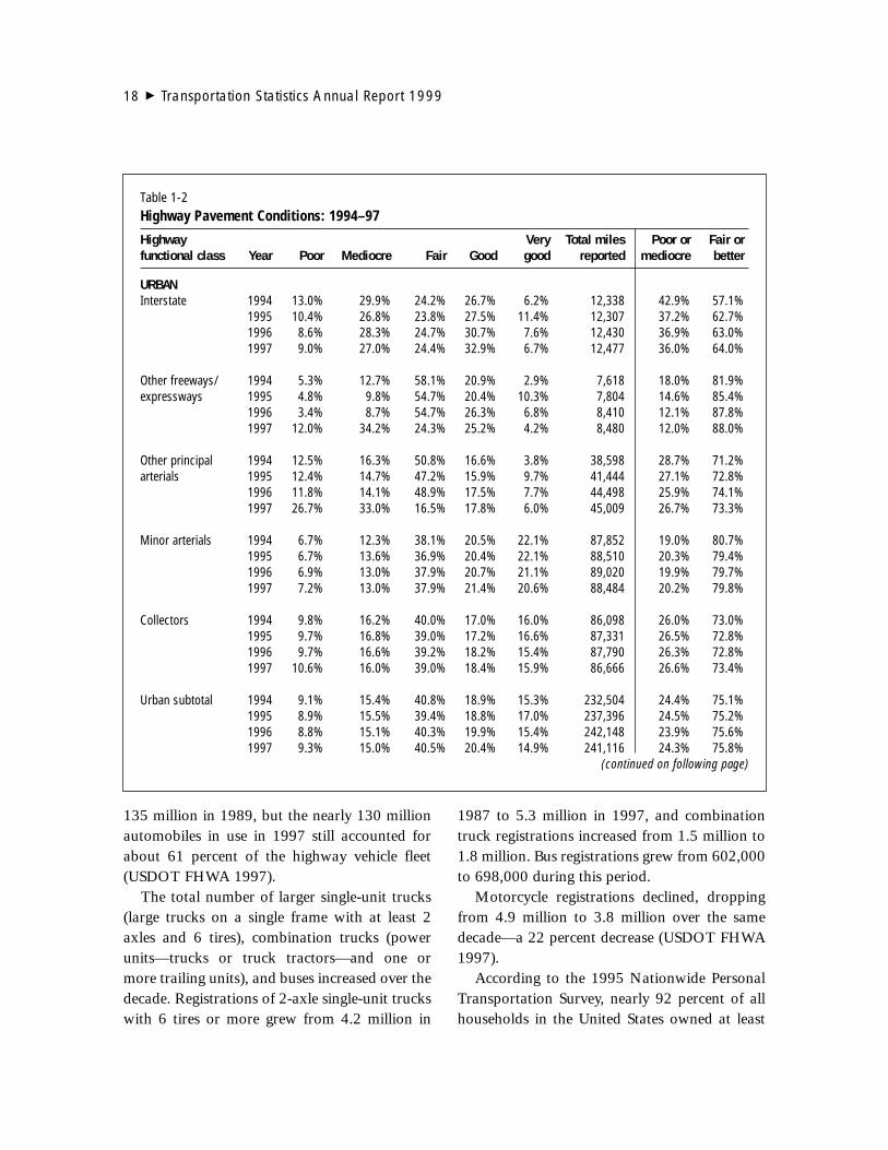
Table 1-2Highway Pavement Conditions: 1994–97
Highway Very Total miles Poor or Fair orfunctional class Year Poor Mediocre Fair Good good reported mediocre better
URBANInterstate 1994 13.0% 29.9% 24.2% 26.7% 6.2% 12,338 42.9% 57.1%
1995 10.4% 26.8% 23.8% 27.5% 11.4% 12,307 37.2% 62.7%1996 8.6% 28.3% 24.7% 30.7% 7.6% 12,430 36.9% 63.0%1997 9.0% 27.0% 24.4% 32.9% 6.7% 12,477 36.0% 64.0%
Other freeways/ 1994 5.3% 12.7% 58.1% 20.9% 2.9% 7,618 18.0% 81.9%expressways 1995 4.8% 9.8% 54.7% 20.4% 10.3% 7,804 14.6% 85.4%
1996 3.4% 8.7% 54.7% 26.3% 6.8% 8,410 12.1% 87.8%1997 12.0% 34.2% 24.3% 25.2% 4.2% 8,480 12.0% 88.0%
Other principal 1994 12.5% 16.3% 50.8% 16.6% 3.8% 38,598 28.7% 71.2%arterials 1995 12.4% 14.7% 47.2% 15.9% 9.7% 41,444 27.1% 72.8%
1996 11.8% 14.1% 48.9% 17.5% 7.7% 44,498 25.9% 74.1%1997 26.7% 33.0% 16.5% 17.8% 6.0% 45,009 26.7% 73.3%
Minor arterials 1994 6.7% 12.3% 38.1% 20.5% 22.1% 87,852 19.0% 80.7%1995 6.7% 13.6% 36.9% 20.4% 22.1% 88,510 20.3% 79.4%1996 6.9% 13.0% 37.9% 20.7% 21.1% 89,020 19.9% 79.7%1997 7.2% 13.0% 37.9% 21.4% 20.6% 88,484 20.2% 79.8%
Collectors 1994 9.8% 16.2% 40.0% 17.0% 16.0% 86,098 26.0% 73.0%1995 9.7% 16.8% 39.0% 17.2% 16.6% 87,331 26.5% 72.8%1996 9.7% 16.6% 39.2% 18.2% 15.4% 87,790 26.3% 72.8%1997 10.6% 16.0% 39.0% 18.4% 15.9% 86,666 26.6% 73.4%
Urban subtotal 1994 9.1% 15.4% 40.8% 18.9% 15.3% 232,504 24.4% 75.1%1995 8.9% 15.5% 39.4% 18.8% 17.0% 237,396 24.5% 75.2%1996 8.8% 15.1% 40.3% 19.9% 15.4% 242,148 23.9% 75.6%1997 9.3% 15.0% 40.5% 20.4% 14.9% 241,116 24.3% 75.8%
(continued on following page)

Chapter 1 System Extent and Condition � 19
Table 1-2Highway Pavement Conditions: 1994–97 (continued)
Highway Very Total miles Poor or Fair orfunctional class Year Poor Mediocre Fair Good good reported mediocre better
RURALInterstates 1994 6.5% 26.5% 23.9% 33.2% 9.9% 31,502 33.0% 67.0%
1995 6.2% 20.7% 22.3% 36.9% 13.9% 31,254 26.9% 73.1%1996 3.9% 19.1% 21.7% 38.8% 16.6% 31,312 23.3% 76.6%1997 3.6% 19.1% 20.7% 41.0% 15.7% 31,431 22.7% 77.3%
Other principal 1994 2.4% 8.2% 57.4% 26.6% 5.4% 89,506 10.6% 89.4%arterials 1995 4.4% 7.6% 51.1% 27.9% 9.0% 89,265 12.0% 88.0%
1996 1.4% 5.8% 49.1% 34.4% 9.3% 92,103 7.4% 92.6%1997 1.6% 4.9% 47.7% 37.2% 8.6% 92,170 6.5% 93.5%
Minor arterials 1994 3.5% 10.5% 57.9% 23.6% 4.5% 124,877 14.0% 86.0%1995 3.7% 9.0% 54.7% 23.9% 8.7% 121,443 12.7% 87.3%1996 2.3% 8.2% 50.7% 31.0% 7.7% 126,381 10.6% 89.4%1997 2.3% 6.7% 50.4% 33.6% 7.0% 126,525 9.0% 91.0%
Major collectors 1994 6.5% 11.3% 33.5% 16.1% 21.9% 431,111 17.8% 71.5%1995 6.5% 11.4% 30.8% 17.4% 23.7% 431,712 17.9% 71.9%1996 6.7% 10.3% 34.4% 20.0% 18.4% 432,117 19.8% 70.1%1997 7.8% 12.3% 37.6% 23.0% 19.3% 386,122 20.1% 79.9%
Rural subtotal 1994 5.4% 11.4% 40.7% 19.7% 16.0% 676,996 16.9% 76.3%1995 5.7% 10.4% 38.1% 20.1% 18.8% 643,749 16.1% 77.0%1996 5.0% 9.7% 38.8% 24.8% 14.8% 681,913 14.7% 78.4%1997 5.6% 10.4% 40.8% 28.1% 15.1% 636,248 16.0% 84.0%
URBAN AND RURAL1994 6.3% 12.4% 40.7% 19.5% 15.8% 909,500 18.8% 76.0%1995 6.6% 11.8% 38.4% 19.8% 18.3% 881,145 18.4% 76.5%1996 6.0% 11.2% 39.2% 23.5% 15.2% 924,061 17.2% 79.2%1997 6.6% 11.7% 40.7% 26.0% 15.0% 877,364 18.3% 81.7%
NOTES: Numbers may not total due to rounding. Condition for rural and urban Interstates and other principal arterials, urban other freeways and expressways,and rural minor arterials based on International Roughness Index data from the Federal Highway Administration. Condition for urban minor arterials and col-lectors and rural major collectors based on Present Serviceability Rating data from the Federal Highway Administration.
KEY: Poor = needs immediate improvement. Mediocre = needs improvement in the near future to preserve usability. Fair = will likely need improvement in thenear future, but depends on traffic use. Good = in good condition; will not require improvement in the near future. Very good = new or almost new pavement;will not require improvement for some time.
SOURCES: U.S. Department of Transportation, Federal Highway Administration, Highway Statistics (Washington, DC: Annual editions), tables HM-63 and HM-64. U.S. Department of Transportation, Bureau of Transportation Statistics, National Transportation Statistics 1999 (Washington, DC: Forthcoming).

one vehicle in that year, with an average of about1.8 vehicles per household. Households withoutat least one vehicle fell from about 11.5 million(15 percent of all households) in 1977 to about8 million (8 percent of households) in 1995.Nearly one-fifth of low-income households(those earning less than $25,000 per year) hadno vehicle in 1995 (ORNL 1999, 7, 9, 28, 29).
The cars and trucks driven in the UnitedStates are older now, on average, than a decadeor so ago. The median age of an automobile in1997 was 8.1 years, compared with 6.9 years in
1987 and 5.6 years in 1977. Median truck ageincreased to 7.8 years in 1997, compared with7.6 in 1987 and 5.7 in 1977.1 (Polk 1999;USDOT BTS 1998, table 1-37). Although it isthe only national indicator available, age is notnecessarily a good indicator of vehicle condition,as the median age of vehicles is affected by manyfactors, including changes in vehicle quality,vehicle costs, and overall economic conditions.
20 � Transportation Statistics Annual Report 1999
Table 1-3Highway Bridge Conditions: 1990 and 1997
Percentage Percentage Percentage Percentage Percentage PercentageFunctional structurally functionally in good Total structurally functionally in good Totalcategory deficient obsolete condition bridges deficient obsolete condition bridges
RURALPrincipal arterials—
Interstates 5.2 20.9 73.9 29,076 4.5 12.2 83.3 28,073Principal arterials—
Other 8.4 14.9 76.7 32,169 7.0 10.7 82.3 34,813Minor arterials 14.1 14.5 71.3 40,927 10.4 11.8 77.9 38,401Major collectors 19.5 13.3 67.2 103,979 13.4 10.4 76.2 95,751Minor collectors 23.2 16.0 60.8 48,797 17.0 10.9 72.1 47,390Local roads 38.1 15.2 46.7 208,487 26.1 11.3 62.6 210,678Total rural 26.1 15.1 58.8 463,435 18.4 11.1 70.5 455,106
URBANPrincipal arterials—
Interstates 9.9 30.2 60.0 24,435 7.4 19.4 73.2 27,142Principal arterials—
other freeways/expressways 9.2 32.0 58.8 11,890 7.0 20.1 72.9 15,170
Other principal arterials 15.9 27.0 57.1 21,403 11.9 21.7 66.4 23,297
Major arterials 17.4 29.0 53.7 18,580 13.4 25.3 61.3 23,300Collectors 20.2 29.0 50.8 11,876 15.2 23.4 61.4 14,939Local roads 21.0 21.7 57.3 20,586 15.1 17.6 67.3 24,780Total urban 15.5 27.8 56.7 108,770 11.6 21.0 67.3 127,628
URBAN AND RURAL 24.1 17.5 58.4 572,205 16.9 13.3 69.8 582,734
SOURCE: U.S. Department of Transportation, Federal Highway Administration, National Bridge Inventory Database, 1998.
1990 1997
1 Median truck age is based on the ages of all trucks, includ-ing light-duty trucks.

RAIL
In 1997, there were nine Class I freight railroads(railroads with operating revenues of $256.4 mil-lion or more) in the United States. These railroadsaccounted for 71 percent of the industry’s171,285 miles operated, 89 percent of its approx-imately 201,000 employees, and 91 percent of its$35.3 billion in freight revenue. There were 34regional railroads (those with operating revenuesbetween $40 million and $256.4 million and/oroperating at least 350 miles of road). The region-al railroads operated 21,466 miles, had about11,000 employees, and earned $1.6 billion in
freight revenue. There were 507 local railroads(falling below the regional railroad threshold,and including switching and terminal railroads)operating over 28,149 miles of road. They hadslightly under 12,000 employees and earned $1.4billion in freight revenue (AAR 1998, 3).
These freight railroads maintain their tracks,rights-of-way, and fleets of railcars and locomo-tives. Over the years, through mergers and ratio-nalization of their physical plants, many little-usedlines were abandoned or sold to smaller railroads.Since 1980, the Class I railroads increased theirtraffic (measured in ton-miles) by 47 percent,while their network (miles of road owned)declined by 38 percent (AAR 1998, 6, 44). Traffic
Chapter 1 System Extent and Condition � 21
1950 1960 1970 1980 1990 1997P0
0.5
1.0
1.5
2.0
2.5
3.0
3.5
4.0
4.5Million miles
Figure 1-1Urban and Rural Roadway Mileage by Surface Type: 1950–97
KEY: P = preliminary.
SOURCES: U.S. Department of Transportation, Federal Highway Administration, HighwayStatistics (Washington, DC: Annual editions),table HM.______. Highway Statistics Summary to 1995(Washington, DC: 1997), table HM-212. Rural, unpaved
Rural, paved
Urban, unpaved
Urban, paved
1987 1988 1989 1990 1991 1992 1993 1994 1995 1996 1997P0
0.2
0.4
0.6
0.8
1.0
1.2
1.4
1.6
1.8
Passenger cars
2-axle 4-tire trucks1
Motorcycles
Buses
Other single-unit trucks2
Combinationtrucks
Number of vehicles
Figure 1-2Registered Highway Vehicle Trends: 1987–97Index: 1987 = 1.0
1 Includes vans, light trucks, and sport utility vehicles.2 Includes all single-unit trucks with at least 2 axles and 6 tires.
KEY: P = preliminary.
SOURCES: 1987–95: U.S. Department of Transportation, Federal Highway Administration. Highway Statistics Summary to 1995 (Washington, DC: 1997), table MV-201 and VM201a.1996–1997: _____. Highway Statistics 1997 (Washington, DC: 1999), table VM-1.

density increased as traffic was concentrated overa smaller network. Because of this increased den-sity, some railroads expanded capacity in theirhighest density corridors by double-tracking, suchas was done by CSX in Ohio in the last few years.In some cases, railroads have even tripled orquadrupled their track on stretches of rail linewhere traffic is very heavy.
As for passenger rail, the National RailroadPassenger Corporation, more widely known asAmtrak, has operated a national passenger sys-tem since May 1971. Amtrak was created by theRail Passenger Service Act of 1971 “. . . to oper-ate a national rail passenger system which tiestogether existing and emergent regional rail pas-senger service and other intermodal passengerservice.” During fiscal year (FY) 1998 (October1, 1997 to September 30, 1998), Amtrak operat-ed more than 250 intercity trains per day along a22,000 route-mile railroad network in 44 stateswith service to more than 500 communities. InFY 1998, Amtrak carried 21.1 million intercitypassengers, generating a total of 5.3 billion pas-senger-miles (up from FY 1996 and FY1997, butstill below other years in the 1990s) and 54 mil-lion commuters carried under contract with tran-sit authorities (NRPC 1998, 47–50). Amtrak alsorelies on an extensive feeder bus network to carryrail passengers to and from off-line locations.
Over the past several years, Amtrak hasordered and taken delivery of about 200 bi-levelSuperliners (designed to replace aging Heritageequipment) and 50 Viewliners servicing theMidwest and the East Coast). The Viewliners arethe first single-level sleeping cars manufacturedin the United States in 40 years. Amtrak alsoreplaced their aging F-40 locomotives with 150nearly new locomotives.
High-speed passenger rail service continues tobuild momentum, albeit slowly. Box 1-1 discuss-es its status in the United States.
AIR
Air transportation is the fastest growing trans-portation mode. Domestic passenger-miles of airtravel more than doubled since 1980, while ton-miles of freight carried by air increased three-fold.2 Airway system mileage increased from341,000 miles in 1980 to 394,000 in 1995; noestimates are available for 1996 and 1997. In1997, the United States had 18,345 airports ofall sizes and descriptions, about 20 percent morethan in 1980. The increase over the period isexplained by the addition of over 3,200 generalaviation airports, which totaled 17,685 in 1997.Certificated airports (those serving scheduled aircarrier operations with aircraft seating morethan 30 passengers), on the other hand, de-creased from 730 in 1980 to 660 in 1997.3 Thisdecline probably reflects the influence of thehub-and-spoke systems used by most major air-lines since airline deregulation in the late 1970s(USDOT BTS 1998, table 1-2).
Airport runway quality improved from 1986to 1997. The percentage of public-use airportswith paved runways increased slightly, as did thepercentage with lighted runways (USDOT BTS1998, table 1-2). Runway pavement quality alsoimproved at the subset of airports listed in theFederal Aviation Administration’s National Planof Integrated Airport Systems (NPIAS). TheNPIAS’s classification of airports includes thosewith commercial service, all reliever airports, andselected general aviation airports. Runways inpoor to fair condition dropped from 39 percentin 1986 to 28 percent in 1997, while those ingood condition rose from 61 percent to 72 per-
22 � Transportation Statistics Annual Report 1999
2 Travel and freight estimates apply to large U.S. air carriersthat file Form 41 with BTS’s Office of Airline Information,rather than the entire certificated fleet.3 The number of certificated airports differs from that for air-ports serving large certificated carriers shown in table 1-1.

Chapter 1 System Extent and Condition � 23
In recent years, high-speed rail (HSR) service forintercity passengers has experienced renewed interest.Several parts of the country have produced HSR plansand some corridors are undertaking development activ-ities (see map). Section 1010 of the Intermodal SurfaceTransportation Efficiency Act of 1991 authorized fundingfor elimination of grade-crossing hazards in designatedHSR corridors. The provision was continued in Section104(c) of the Transportation Equity Act for the 21stCentury (TEA-21) of 1998.
Northeast and Empire CorridorsThe Northeast Corridor (NEC) handles approximate-
ly half of Amtrak’s intercity passengers. Amtrak planshigh-speed passenger service along the entire NECbetween Washington, DC, and Boston. Its goal is to re-duce travel times to 3 hours between New York City andBoston and 21⁄2 hours between Washington, DC, andNew York City. When an overhead electric power supplysystem, known as a catenary, between New Haven,Connecticut, and Boston is completed in 2000, all 456miles of the NEC will be electrified. Other infrastructureinvestments needed to meet the trip-time goals includeadditional tracks to separate high-speed intercity trainsfrom slower commuter operations, straightening curveswithin the boundaries of existing rights-of-way, andmodernization of train control systems. Amtrak plans toplace 20 high-speed (up to 150 miles per hour—mph)all-electric trainsets in service along the NEC by the endof 2000.
TEA-21 designated the “Empire Corridor” from NewYork to Albany and on to Buffalo as a high-speed corri-dor under Section 1103(c). In late 1998, Amtrak officialsand New York’s Governor announced a 5-year, $185 mil-lion plan to upgrade the New York City/Albany/Buffaloline and rebuild trains used on the route. Travel times forthe 141-mile New York City-Albany trip could bereduced to under 2 hours. A second track will be builtbetween Albany and Schenectady, and the trackbetween Albany and Buffalo will be upgraded, cutting asmuch as 1 hour off the 71⁄2-hour trip between New YorkCity and Buffalo.
California CorridorCalifornia has spent or committed nearly $800 mil-
lion to upgrade the San Francisco-Oakland-Sacramento-Los Angeles-San Diego Corridor, near which 90 percentof the state’s population lives. This HSR corridor con-
tains approximately 600 at-grade crossings. The statehas received $5.7 million in federal funds to closeredundant crossings and upgrade the corridor’s otherpublic and private crossings. Amtrak plans to acquireeight trainsets to be used in Amtrak’s San Diegan ser-vice from San Diego to Los Angeles, Santa Barbara, andSan Luis Obispo.
California’s High Speed Rail Authority is preparing astate plan for HSR for the Governor and the legislature.Its predecessor, the California Intercity High-Speed RailCommission, had recommended two options for a 676-mile statewide HSR network. One would cost $23.3 bil-lion, the other (a magnetic levitation system) $31.6billion—public works projects on a scale with California’sfreeway system. In February 1999, the Authority decidedon a less ambitious HSR plan. It proposed a very high-speed (186 mph) grade-separated service only from LosAngeles to San Francisco. San Diego, Sacramento, andother system routes would be served by a high-speedfeeder network operating at 100 mph.
Pacific Northwest Corridor (Cascadia)The Pacific Northwest Corridor extends from
Eugene, Oregon, to Vancouver, British Columbia.Washington State’s Department of Transportation andAmtrak have purchased four high-speed trainsets,which are now operating in the corridor.
Chicago Hub Network• Midwest Regional Rail Initiative. In August 1998, ninemidwestern states released an HSR corridor study. Thestudy found that, by upgrading routes now in place andusing diesel multiple unit power, speeds of up to 110mph could be achieved at a cost of about $3.5 billion toupgrade the tracks and signals and to purchase equip-ment. The plan would take about six years to implement.The plan has a positive benefit to cost and operatingratio. The states are seeking funding to continue workon HSR.• Detroit-Chicago Segment. Michigan is demonstratingan advanced communications-based train control sys-tem on an 80-mile section of the Detroit-Chicago corri-dor. The system ensures safe distances between trainsoperating at speeds of up to 100 mph. (See box 1-3 laterin the chapter for details.)• St. Louis-Chicago Segment. Six miles of Union Pacifictrack are being rehabilitated to provide a less congested
Box 1-1High-Speed Rail Corridor Status
(continued on following page)

24 � Transportation Statistics Annual Report 1999
=
=
=
=
Designated High-Speed Rail CorridorsVancouver, BC
Bellingham
SeattleTacoma
PortlandSalem
Eugene
SacramentoStockton
Fresno
Bakersfield
Los Angeles
San Diego
St. Louis
Springfield
Chicago
Milwaukee
La Crosse
Minneapolis
KalamazooDetroit
Rochester
Buffalo
Baltimore PhiladelphiaTrenton
New YorkNew Haven
Providence
Boston
Richmond
Washington DC
Harrisburg
DurhamGreensboro
CharlotteGreenville
AtlantaBirmingham
Meridian
Mobile
New Orleans
Tampa
LakelandOrlando
Jacksonville
Savannah
Columbia
Miami
West Palm Beach
HoustonBiloxi
Macon
Raleigh
Hampton
Albany
Porter
Indianapolis
Cincinnati
East St. Louis
Bay Area
Olympia
KEY: ISTEA = Intermodal Surface Transportation Equity Act of 1991; TEA-21 = Transportation Equity Act for the 21st Century.
SOURCE: U.S. Department of Transportation, Federal Railroad Administration, 1999.
High-speed rail corridors
ISTEATEA-21Northeast
PacificNorthwestCorridor
Chicago Hub
Empire Corridor
NortheastCorridor
SoutheastCorridor
FloridaCorridor(state funding discontinued)
Gulf CoastCorridor
CaliforniaCorridor
alternative route across the Mississippi River into St.Louis. Amtrak trains would be rerouted to achieve moredirect access to the St. Louis terminal and to reducemixing of freight and passenger traffic. The current trav-el time would be reduced by more than 20 minutes andon-time performance would be improved.
Southeast CorridorIn late 1998, the Southeast Corridor partnership
between North Carolina and Virginia was expanded toinclude South Carolina, Georgia, and Florida. The inten-tion of the new partnership is to develop an HSR corri-dor connecting Charlotte, Raleigh, and Richmond withthe high-speed Northeast Corridor (beginning in Wash-ington, DC), as well as major travel markets of the
Southeast. It could cost $1.1 billion to upgrade the en-tire corridor from Charlotte to Washington.
Another candidate for HSR service is the Richmondto Tidewater area of Virginia. The Virginia MajorInvestment Study recommends that the rail corridor bedouble-tracked with track and signal improvements toallow train speeds up to 110 mph, with 8 roundtrips perday, and 3 new train stations. These improvementscould cost $256 million and would be part of a largerpackage of transportation corridor improvements(including a third highway lane and interchange andother highway improvements) that would cost an esti-mated $1.34 billion).
SOURCE: U.S. Department of Transportation, Federal RailroadAdministration.
Box 1-1High-Speed Rail Corridor Status (continued)

cent. Airport runway conditions at commercialservice airports, a subset of the NPIAS, haveremained nearly static, though, with 79 percent ingood condition in 1997. The remaining 21 per-cent of commercial airport runways were classi-fied as poor or fair (USDOT BTS 1998, table1-36). Still, overall commercial airport runwaysremain in better condition than NPIAS airports.
The number of aircraft operated by certificat-ed air carriers increased from 7,320 in 1992 to7,616 in 19974 (USDOT FAA 1999b). Totals forthe entire certificated fleet are not available foryears prior to 1992, though growth is evident forthe portion of the fleet for which pre-1992 dataare available.
The general aviation fleet consisted of over192,000 active aircraft in 1997, the third consec-utive year of increase. A decline in the fleetoccurred between 1989 and 1994—from205,000 aircraft to 172,000 aircraft. General avi-ation aircraft are flown for a variety of purposes.The most popular is personal use (60 percent),followed by business (14 percent), instruction (8percent), and corporate activities (5 percent),with smaller portions of the fleet used for airtours, sightseeing, air taxi, and other applica-tions. Most active general aviation aircraft (52percent of those whose ages are known) are 25years old or less, 40 percent are between 26 and50 years old, and 8 percent are over 50 years old(USDOT FAA 1999a; USDOT FAA 1998).
WATER
U.S. water ports handled approximately 2.3 bil-lion tons of foreign and domestic waterbornecommerce in 1997 (USACE 1997). Internationalshipments increased by one-third between 1980and 1997, while domestic shipments—coastwise,
inland, and on the Great Lakes—increased verylittle. About 27 percent of the world merchantfleet called at U.S. ports in 1997, representing 44percent of the world’s dead-weight-tonnagecapacity (USDOT BTS MARAD USCG Forth-coming).
The port and waterway system plays animportant role in recreation and tourism. Of the223 large cruise ships in the world fleet, abouthalf (109) call regularly at U.S. ports. In addi-tion, recreational boating is a major activity.Approximately 12.3 million recreational boatswere numbered (registered) in the United Statesin 1997, compared with 10 million in 1987 and8 million in 1977. Numbered recreational boatsincreased by 441,000 in 1997, the most growthin a single year since 1988. An unknown numberof other boats are not registered (USDOT BTSMARAD USCG Forthcoming).
In the United States, 25,000 miles of commer-cially navigable waterways serve 41 states,including all states east of the Mississippi River(USACE 1999a). Hundreds of locks facilitatetravel along these waterways. The U.S. ArmyCorps of Engineers owned or operated 276 lockchambers at 230 sites in 1997, with lifts rangingfrom 5 to 49 feet on the Mississippi River and upto 110 feet at the John Daly Lock on theColumbia River (USACE 1999b, 1999c). InJanuary 1999, 135 of the 276 chambers hadexceeded their 50-year design lives. The oldestoperating locks in the United States, KentuckyRiver Locks 1 and 2, were built in 1839 (USACE1999c).
U.S. ports, or marine terminals, function asintermodal freight connections between watervessels and highway and rail networks. In 1997,the nation’s marine terminals were nearly equal-ly divided in number among deep-draft (oceanand Great Lake) and shallow-draft (inlandwaterway) facilities with 1,914 located along thecoasts (including Alaska, Hawaii, Puerto Rico,
Chapter 1 System Extent and Condition � 25
4 Air carrier aircraft are aircraft carrying passengers or cargofor-hire under 14 CFR 121 and 14 CFR 135, except for on-demand air taxis.
and the U.S. Virgin Islands) and Great Lakes and1,812 located along inland waterways (USDOTMARAD 1998). Nearly 90 percent of inlandfacilities were privately owned in 1997 com-pared with about two-thirds of coastal facilities.
In 1997, 86 percent of the inland ports wereused primarily for the transfer of bulk commodi-ties such as grain, coal, and petroleum; only 14percent of these ports were general cargo or mul-tipurpose terminals. At coastal terminals, gener-al cargo accounted for 37.5 percent of the berths(including the Great Lakes) and a similar share(41.2 percent) was used for bulk commodities.About 2.8 percent of coastal berths servedpassenger vessels, 11.2 percent served barges, 4.2percent were used for mooring or other purpos-es, and 3 percent were inactive (USDOTMARAD 1998).
Over the next few years, coastal ports will befaced with the challenge of handling the nextgeneration of containerships. Each “megaship”has a capacity of 4,500 20-foot equivalent con-tainer units (TEUs) or more, and drafts of 40 to46 feet when fully loaded. The first of these ves-sels was delivered in 1996, and containershipoperators around the world may take delivery of35 more through 1999. To physically accommo-date megaships at U.S. ports, channel and berthdepths must be at least 50 feet. However, only 5of the top 15 U.S. container ports—Baltimore,Tacoma, Hampton Roads, Long Beach, andSeattle—have adequate channel depths, and onlythose on the west coast have adequate berthdepths. In addition, ports may need to expandterminal infrastructure, such as cranes, storageyards, and information systems, to facilitate theincreased volumes of cargo from these ships.Also, landside modes and facilities connectingwith water terminals will face higher volumes ofrail and truck traffic. Many ports have initiatedexpansion projects to accommodate these ships.How effectively U.S. ports handle this next gen-
eration of containerships will have implicationsfor the efficiency of the U.S. transportation sys-tem and U.S. trade competitiveness (USDOTMARAD 1998, 49–51).
The U.S.-flag commercial vessel fleet in-creased to 41,419 in 1997, compared with38,788 in 1980 (USACE NDC 1999; USACEWRSC 1998). Barges accounted for the over-whelming share—nearly 80 percent of the entirefleet—both in terms of number of vessels andcargo capacity. Tugboat and towboats accountedfor around 12.5 percent of the fleet, and otherself-propelled vessels such as dry cargo ships,cruise ships, tankers, and offshore support ves-sels accounted for the remainder.
Self-propelled vessels, such as tankers, contain-erships, and dry bulk carriers, have larger cargocapacity than barges (see table 1-4). Tankers havethe most capacity—51,000 short tons on average(the largest tankers have a capacity of over262,000 short tons). The average carry of liquidand dry cargo barges was 1,700 short tons.
Cruise ships, gambling/casino boats, and ves-sels reported as employed in sightseeing, excur-sions, and other such activities numbered 1,206in 1997. These vessels had an average capacity of298 passengers. There were 5,713 tugboats/pushboats available to operate or operating dur-ing 1997. Of these, about 32 percent had 500 to1,000 horsepower and were, on average, 26years old, and 17 percent were under 500 horse-power and averaged 34 years of age.5
The average commercial vessel (includingcargo, passenger, and other vessels) in 1997 wasabout 27 years old. Containerships were, in gen-eral, newer than the rest of the fleet, averagingabout 16 years, while dry bulk carriers were theoldest, averaging 28 years. Passenger vessels
26 � Transportation Statistics Annual Report 1999
5 Average capacity calculation excludes two vessels forwhich passenger capacity data were not available; averagecargo capacity calculation excludes 52 vessels for whichcargo capacity data were not available.

averaged about 21 years old. Ferries in operationin the United States averaged about 23 years old.
BTS and two other Department of Trans-portation agencies, the Maritime Administrationand the U.S. Coast Guard, will issue a compre-hensive report on water transportation in late1999 (see box 1-2).
OIL AND GAS PIPELINES
An extensive system of pipelines is in place fortransmission of petroleum, petroleum products,and natural gas throughout the country. Theextent of the network and the amount of pipelineactivity are unclear due to differences in nation-al estimates and gaps in publicly available data.Table 1-1 shows Eno Foundation estimates for
oil pipelines and American Gas Association esti-mates for natural gas pipelines.6
Chapter 1 System Extent and Condition � 27
Table 1-4U.S.-Flag Waterborne Cargo-Carrying Vessel Fleet Profile: 1997
Total cargo capacity Average cargo capacity1 AverageICST codes Vessels (short tons) (short tons) age2
Self-propelled 3 2,209 13,973,152 6,326 22Dry cargo 692 6,191,012 8,947 23
Containership 310 82 2,632,171 32,100 16Dry bulk carrier 229 72 2,529,358 35,130 28General cargo 333,334,335 350 943,899 2,697 27Specialized 321,325,329 188 85,584 455 19
Offshore support 422 1,370 306,120 223 26Tanker 114,120,139,199 147 7,476,020 50,857 23
Non-self-propelled 33,011 54,974,961 1,665 20Dry cargo barge 341-344,349 29,040 43,809,931 1,509 17Tank barge 141-144,149 3,971 11,264,868 2,837 23
1 Average is calculated from only those vessels with known capacity and not the total number of vessels.2 Age is based on the year the vessel was built or rebuilt. Average is calculated from only those vessels with known year built or rebuilt.3 Does not include passenger vessels and towboats.
KEY: ICST = International Classification of Ships by Type.
NOTE: Includes vessels operating or available to operate in 1997.Excludes, for example, fishing and excursion vessels, general ferries and dredges used in construction work.
SOURCE: U.S. Army Corps of Engineers, Navigation Data Center, Waterborne Commerce Statistics Center, Vessel Characteristics Database (New Orleans, LA:1999).
6 Two federal agencies estimate oil and natural gas pipelinemileage: the Federal Energy Regulatory Commission(FERC) and the Office of Pipeline Safety (OPS) in the U.S.Department of Transportation’s Research and SpecialProjects Administration. Their mileage estimates differ,largely due to jurisdictional differences. FERC collects datafor pipelines involved in interstate commerce or those withcontinuous flow, including gathering lines. Operators withan annual revenue of less than $350,000 are excluded. OPS,on the other hand, collects data for all pipelines except gath-ering lines of 6 inches or less in diameter, pipelines owned bycompanies with fewer than 30 miles of pipe nationwide, andgas lines less than 1 mile in length. These criteria are illus-trative and are not complete. Additional criteria determinewhether a pipeline is under FERC and/or OPS jurisdiction.

28 � Transportation Statistics Annual Report 1999
In late 1999, three Department of Transportationadministrations, the Bureau of Transportation Statistics(BTS), the Maritime Administration (MARAD), and theU.S. Coast Guard (USCG) will issue a report, MaritimeTrade & Transportation 1999, which presents informa-tion about maritime transportation in the United Statesand around the world. It covers waterborne trade andtransportation services between 1993 and 1997,reviews trends in U.S. shipbuilding, explores safety andenvironmental issues associated with maritime activitiesand recreational boating, discusses national securityissues and navigation technology, and presents dataneeds. The report also examines capacity trends forthree categories of vessels in deep-sea trade: 1) con-tainerships and other general cargo vessels, 2) dry bulkcarriers, and 3) tankers.
The capacity of the world’s containership fleetincreased dramatically between 1993 and 1997, grow-ing 15 percent per year. The growth was partly due tonewly deployed large containerships (those able to han-dle 4,000 or more 20-foot equivalent container units) ineast/west trade (e.g., between the United States andJapan), which led to the redeployment of smaller ves-sels for north/south intra-regional trade. Dry bulk fleetcapacity grew 4.2 percent per year, while growth intanker fleet capacity was 0.6 percent per year. A grow-ing proportion of the world fleet is owned by partieswhose nationality differs from that of the country inwhich the vessel is registered. In 1993, 50 percent of theworld merchant fleet were in such open registries, whilein 1997, open registries accounted for 57 percent of themerchant fleet. A very different picture of the world fleetappears if flag registry is compared with country of
ownership. Panama, Liberia, Greece, the Bahamas, andMalta are the top five countries by registry, measured intotal dead-weight tonnage, with the United States ranked11th. Tankers accounted for a majority of the U.S.-ownedcapacity. When ownership is the criterion, Japan,Greece, the United States, Norway, and the UnitedKingdom are the top five. However, for containerships,Germany ranks highest by far in ownership, with twicethe dead-weight tonnage of the next two countries(Japan and Taiwan), each with over 5,000 dead-weighttons. Japan led in tanker and dry bulk capacity.
In the area of U.S. domestic waterborne trade,Alaskan crude oil shipments decreased in the 1990s re-sulting in an overall decline in domestic deep-sea ship-ping, even though other categories of shipments grew.Vessels on inland waterways carried 655 million metrictons in 1997. Great Lakes shipping reached 111 millionmetric tons in 1997.
Japan and South Korea are the world’s largest mer-chant shipbuilders, each holding about one-third of themarket, followed by China, which is a distant third. TheUnited States ranks 14th, with about 1 percent of themarket by gross tonnage. Other components of theshipbuilding market include military construction, andship repair and related industries. The major U.S. ship-building and repair base comprises 92 facilities, includ-ing 19 shipbuilding facilities, 33 dry-dock repairfacilities, and 40 topside repair facilities. Although theU.S. shipbuilding industry is large, it traditionallyfocused on military orders, which are lower today thanin the 1980s. Thus, the global market has become animportant strategic opportunity for the U.S. shipbuildingindustry.
Box 1-2Report on Maritime Trade and Water Transportation
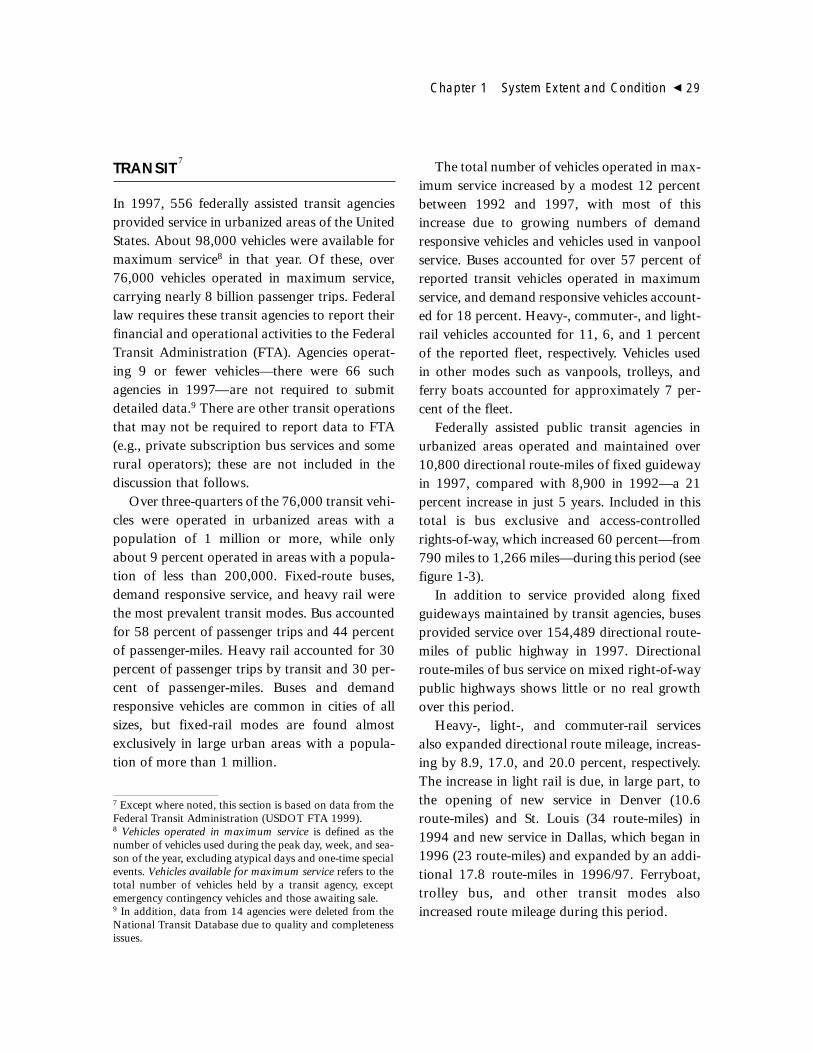
TRANSIT 7
In 1997, 556 federally assisted transit agenciesprovided service in urbanized areas of the UnitedStates. About 98,000 vehicles were available formaximum service8 in that year. Of these, over76,000 vehicles operated in maximum service,carrying nearly 8 billion passenger trips. Federallaw requires these transit agencies to report theirfinancial and operational activities to the FederalTransit Administration (FTA). Agencies operat-ing 9 or fewer vehicles—there were 66 suchagencies in 1997—are not required to submitdetailed data.9 There are other transit operationsthat may not be required to report data to FTA(e.g., private subscription bus services and somerural operators); these are not included in thediscussion that follows.
Over three-quarters of the 76,000 transit vehi-cles were operated in urbanized areas with apopulation of 1 million or more, while onlyabout 9 percent operated in areas with a popula-tion of less than 200,000. Fixed-route buses,demand responsive service, and heavy rail werethe most prevalent transit modes. Bus accountedfor 58 percent of passenger trips and 44 percentof passenger-miles. Heavy rail accounted for 30percent of passenger trips by transit and 30 per-cent of passenger-miles. Buses and demandresponsive vehicles are common in cities of allsizes, but fixed-rail modes are found almostexclusively in large urban areas with a popula-tion of more than 1 million.
The total number of vehicles operated in max-imum service increased by a modest 12 percentbetween 1992 and 1997, with most of thisincrease due to growing numbers of demandresponsive vehicles and vehicles used in vanpoolservice. Buses accounted for over 57 percent ofreported transit vehicles operated in maximumservice, and demand responsive vehicles account-ed for 18 percent. Heavy-, commuter-, and light-rail vehicles accounted for 11, 6, and 1 percentof the reported fleet, respectively. Vehicles usedin other modes such as vanpools, trolleys, andferry boats accounted for approximately 7 per-cent of the fleet.
Federally assisted public transit agencies inurbanized areas operated and maintained over10,800 directional route-miles of fixed guidewayin 1997, compared with 8,900 in 1992—a 21percent increase in just 5 years. Included in thistotal is bus exclusive and access-controlledrights-of-way, which increased 60 percent—from790 miles to 1,266 miles—during this period (seefigure 1-3).
In addition to service provided along fixedguideways maintained by transit agencies, busesprovided service over 154,489 directional route-miles of public highway in 1997. Directionalroute-miles of bus service on mixed right-of-waypublic highways shows little or no real growthover this period.
Heavy-, light-, and commuter-rail servicesalso expanded directional route mileage, increas-ing by 8.9, 17.0, and 20.0 percent, respectively.The increase in light rail is due, in large part, tothe opening of new service in Denver (10.6route-miles) and St. Louis (34 route-miles) in1994 and new service in Dallas, which began in1996 (23 route-miles) and expanded by an addi-tional 17.8 route-miles in 1996/97. Ferryboat,trolley bus, and other transit modes alsoincreased route mileage during this period.
Chapter 1 System Extent and Condition � 29
7 Except where noted, this section is based on data from theFederal Transit Administration (USDOT FTA 1999).8 Vehicles operated in maximum service is defined as thenumber of vehicles used during the peak day, week, and sea-son of the year, excluding atypical days and one-time specialevents. Vehicles available for maximum service refers to thetotal number of vehicles held by a transit agency, exceptemergency contingency vehicles and those awaiting sale.9 In addition, data from 14 agencies were deleted from theNational Transit Database due to quality and completenessissues.
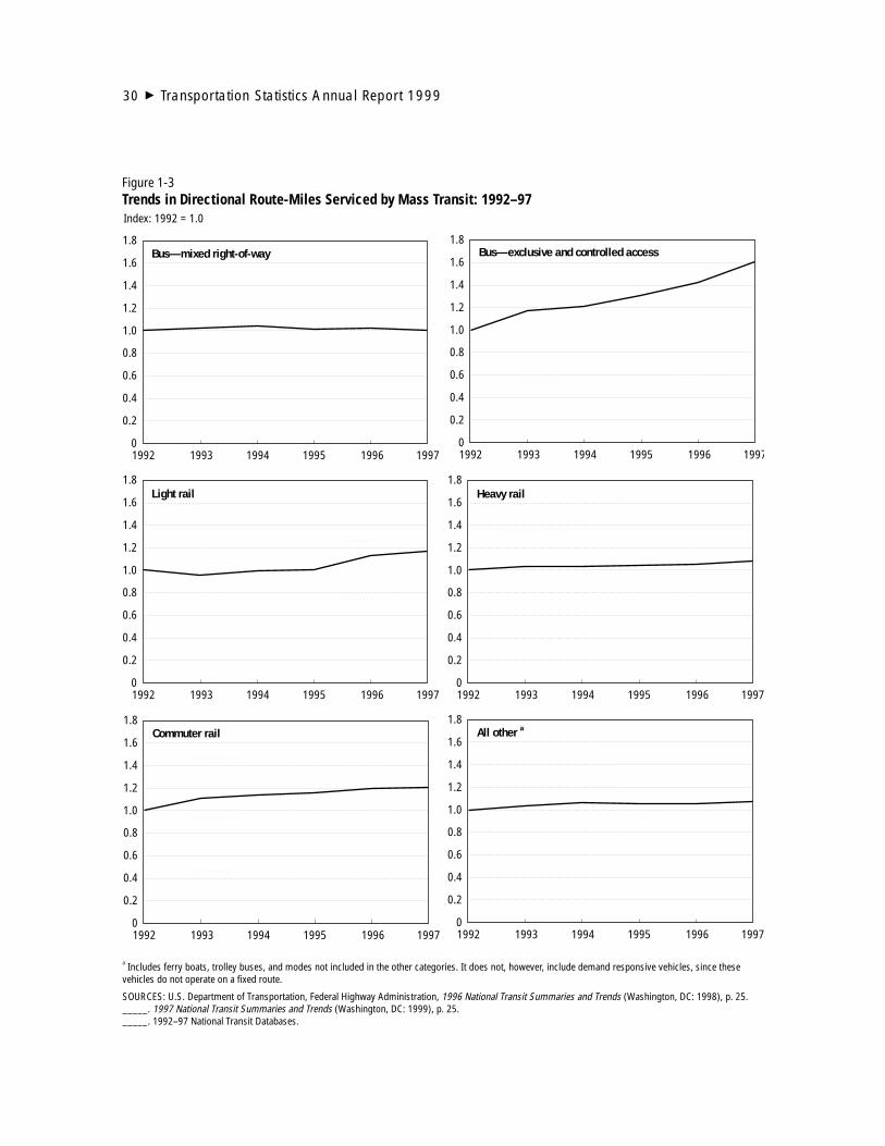
30 � Transportation Statistics Annual Report 1999
Heavy railLight rail
1992 1993 1994 1995 1996 19970
0.2
0.4
0.6
0.8
1.0
1.2
1.4
1.6
1.8Bus—exclusive and controlled access
Commuter rail
1992 1993 1994 1995 1996 19970
0.2
0.4
0.6
0.8
1.0
1.2
1.4
1.6
1.8
1992 1993 1994 1995 1996 19970
0.2
0.4
0.6
0.8
1.0
1.2
1.4
1.6
1.8
1992 1993 1994 1995 1996 19970
0.2
0.4
0.6
0.8
1.0
1.2
1.4
1.6
1.8
Bus—mixed right-of-way
1992 1993 1994 1995 1996 19970
0.2
0.4
0.6
0.8
1.0
1.2
1.4
1.6
1.8
1992 1993 1994 1995 1996 19970
0.2
0.4
0.6
0.8
1.0
1.2
1.4
1.6
1.8
Index: 1992 = 1.0
Figure 1-3Trends in Directional Route-Miles Serviced by Mass Transit: 1992–97
All other a
a Includes ferry boats, trolley buses, and modes not included in the other categories. It does not, however, include demand responsive vehicles, since thesevehicles do not operate on a fixed route.
SOURCES: U.S. Department of Transportation, Federal Highway Administration, 1996 National Transit Summaries and Trends (Washington, DC: 1998), p. 25._____. 1997 National Transit Summaries and Trends (Washington, DC: 1999), p. 25._____. 1992–97 National Transit Databases.
There were approximately 5,000 other transitagencies in existence in 1997. About 4,000 ofthese were federally assisted with 1,000 servingrural areas (Section 18 operators) and 3,500 pro-viding service to people with special needs(Section 16 operators) (APTA 1999).
The average age of transit vehicles overall wasstable between 1992 and 1997, largely becausebuses, the most numerous vehicle type, showedlittle change. The average age of buses in 1997was 8.1 years, compared with 8.3 in 1992.Demand responsive vehicles averaged 3.4 years,the same as in 1992 although the averageincreased to 3.7 in 1993/94. The average age oflight-rail vehicles was 15.9 years in 1997, com-pared with 17.1 years in 1992. Commuter railand heavy rail, on average, have the oldest vehi-cles, and during this period show the mostincrease in average age. The average age of com-muter-rail vehicles rose by 2.1 years to 20.6, andheavy rail increased from 17.8 to 21.1 years.
INFORMATION TECHNOLOGY USEIN TRANSPORTATION
Railroading, aviation, and marine navigation haveactively used information technologies (IT) toenhance the capabilities of the transportation sys-tem, as evidenced by the rapid diffusion of trans-portation applications for such innovations as thetelegraph in the 19th century, and radio and radarin the first half of the 20th century. (Box 1-3 dis-cusses innovative applications for IT in the rail-road industry.) Advances in telecommunicationsand computer hardware and software allow allmodes of transportation access to IT applications,including highways and transit, which previouslyused information and communications technolo-gies less intensively than other modes.
Intelligent transportation systems (ITS),which comprise a broad range of technologies,help to improve the efficiency and effectiveness
of transportation. Electronic surveillance, com-munications, and traffic analysis and controltechnologies provide information and guidanceto transportation system users and help trans-portation agencies monitor, route, control, anddisseminate information.
ITS for highway and transit is in the earlystages of implementation. Particular goalsinclude improving safety, reducing travel time,and easing delay and congestion. Tracking ofdeployment is complicated by the variety of tech-nologies and approaches that could be classifiedas ITS. However, implementation is expanding,especially in larger urban areas troubled by traf-fic congestion. A federal survey of ITS in 78 ofthe largest cities in the United States was con-ducted between the summer of 1997 and thesummer of 1998. Data were collected on deploy-ment of nine components of ITS infrastructurefor highways, transit, and highway-rail gradecrossings within the boundaries of the metropol-itan planning organizations (MPOs) for theselarge metropolitan areas (see figure 1-4). Severaltechnologies or approaches could be utilized in asingle component.
Global Positioning Systems (GPS) are in use innumerous transportation modes (even walking),although to what extent is uncertain. For theMPOs surveyed above, 23 percent showed somedeployment of automatic vehicle location devicesin fixed-route or light-rail transit vehicles. In1996, the U.S. Coast Guard brought itsDifferential GPS online. Reference stations locat-ed every 200 miles along the coast and majorrivers allow ships with the proper GPS receivingequipment to identify their positions within 5 to10 meters, compared with 100 meters for otherpositioning systems. This is an important navi-gational aid, as some channels are less than 100meters wide.
GPS is used for both commercial and generalaviation. About 70 percent of corporate and
Chapter 1 System Extent and Condition � 31

over half of business-use aircraft have GPSdevices, compared with about 40 percent of per-sonal-use aircraft (USDOT FAA Forthcoming,table 7.2).
DATA NEEDS
Information about the extent of the nation’stransportation infrastructure and vehicle fleet isfairly complete for most modes. However, pub-
licly available data for gas and liquid pipelinesdiffer among sources, and accurate, national-level estimates of the pipeline inventory are notavailable on an annual basis. Transit vehicleinformation from public agencies that do notreport to FTA is limited, yet these agencies pur-chase or support sizable amounts of transit ser-vices. Few national data are available about thenumber of small, rural transit providers andorganizations that provide transit as a secondary
32 � Transportation Statistics Annual Report 1999
In an era of growing rail traffic and increased inter-est in high-speed rail passenger service, several ongo-ing projects suggest the importance of informationtechnologies (IT) for railroad safety. IT is at the heart ofmany train control concepts, aimed at reducing theprobability of collisions between trains while increasingtrack capacity and asset use. At least 13 projects are atvarious stages of implementation in the United Statesand Canada, a few of which are described below.
The states of Oregon and Washington, in partnershipwith the Federal Railroad Administration (FRA) andBurlington Northern Santa Fe and Union Pacific rail-roads, are testing new Positive Train Separation tech-nology. The system, which uses global positioningsatellites and land-based transponders, is being testedfor reliability and the ability to safely provide morecapacity on the existing rail infrastructure. When opera-tional, the system may enable passenger trains to oper-ate faster than the current 79 mph speed limit. Acommunications system being developed as part of theproject would carry control signals between trains andrailroad dispatch centers. Testing of the prototype hasverified the reliability of digital communications links,automatic location systems based on the DifferentialGlobal Positioning System (DGPS), and the perfor-mance of an adaptive braking system governed by anonboard computer to determine safe braking distances.
Michigan’s Department of Transportation (MDOT) isinstalling and demonstrating an advanced communica-tions-based train control system on an 80-mile segmentof the Amtrak-owned portion of the Detroit-Chicago cor-ridor between Kalamazoo, Michigan, and the Indianastate line. MDOT and Amtrak matched the federal funds
to upgrade the track so that trains can operate at speedsof up to 110 mph and to make fencing and stationimprovements. As a first step, a 100 mph test of anIncremental Train Control System (ITCS) was conduct-ed on a 20-mile section. Revenue service could begin in2000, and will be coordinated with local freight opera-tions on the line.
The ITCS uses digital radio to broadcast status infor-mation to the train. An onboard computer combinesinformation from the DGPS, wayside status information,and data from an onboard route database to inform theengineer of safe operating speeds. The onboard com-puter acts to stop the train if unsafe operation isattempted. The onboard computer also uses the digitalradio links to activate highway grade-crossing warningsystems at the appropriate time for the approach of thehigh-speed train, and confirms the readiness of thecrossing systems back to the train.
In a portion of the Chicago-St. Louis corridor, thestate of Illinois, FRA, and major freight railroads repre-sented by the Association of American Railroads areconducting a joint demonstration of a Positive TrainControl system expected to cost about $60 million overfour years. The program will address interoperabilityissues among the various railroads, as well as result ina demonstration system. The demonstration system willuse DGPS onboard locomotives, digital radio, andadvanced computers to monitor the location of trains inthe rail system and oversee operation by locomotiveengineers to prevent collisions and overspeed derail-ments. The system on the Chicago-St. Louis corridorwill be controlled from Union Pacific’s HarrimanDispatch Center in Omaha.
Box 1-3Railroad Applications for Information Technology
service (e.g., shuttle and dial-a-ride services pro-vided by hotels, airports, universities, and oth-ers). Also, as ITS evolves and its implementationbecomes more extensive, it will become impor-tant to have a comprehensive inventory of thistechnology across the nation.
Information about the condition of trans-portation vehicles and infrastructure is spottyand uncertain. Condition data for highways,
bridges, and airport runways have a long histo-ry, but for other infrastructure as well as for vehi-cles, vessels, and aircraft, age is one of the fewindicators available, and few age data exist.Also, as the quality and expected lifetime of thesetransportation elements often change, andbecause other factors affect new vehicle sales,age alone is an inadequate measure.
Chapter 1 System Extent and Condition � 33
0
10
20
30
40
50
60
70
80
90
100
1723
11
18
36
23
43
22
5
15
Freew
ay
manag
emen
tInc
ident
manag
emen
t—
freew
ay Incide
nt
manag
emen
t—
arteri
al
Traffic
sign
al
contr
ol
Electr
onic
toll
colle
ction Tra
nsit
manag
emen
t
Electr
onic
fare
paym
ent
Emerg
ency
manag
emen
t
Highway
-rail
grade
cros
sings
Region
al mult
imod
al
trave
ler in
formati
on
Percentage of deployment opportunity
Figure 1-4Indicators of Intelligent Transportation System Infrastructure Deployment: Fiscal Year 1997
NOTE: These percentages describe the amount of deployment relative to total deployment potential (e.g., a city that has 10 miles of its 100 miles of freeway covered by incident detection systems would have a 10% deployment rate). It should be noted that deployment opportunity describes the total deployment potential and does not necessarily represent implementation goals or a specified level of need.
SOURCE: U.S. Department of Transportation, Federal Highway Adminstration, Intelligent Transportation Systems Joint Program Office, Tracking the Deployment of the Integrated Metropolitan Intelligent Transportation Systems Infrastructure in the USA: FY 1997 Results (Washington, DC: 1998), p. ES-2.

REFERENCES
American Public Transit Association (APTA). 1999.Available at www.apta.com/stats/index.htm.
Association of American Railroads (AAR).1998. Railroad Facts. Washington, DC.
National Railroad Passenger Corp. (NRPC). 1998.Amtrak Annual Report. Washington, DC.
Oak Ridge National Laboratory (ORNL). 1999.Summary of Travel Trends: 1995 NationwidePersonal Transportation Survey. Oak Ridge, TN.
Penn Well Publishing Co. 1998. Oil & GasJournal 96:35. Tulsa, OK.
R.L. Polk Co. 1999. Personal communication.
U.S. Army Corps of Engineers (USACE). 1997.Waterborne Commerce of the United States,Calendar Year 1996; Part 5—NationalSummaries. New Orleans, LA: U.S. ArmyEngineer District.
____. 1999a. Internet website. Available at www.wrsc.usace.army.mil/ndoooc/fcdidu3.htm.
____. 1999b. 1997 Lock Characteristics Data-base. Available at www.wrsc.usace.army mil/ndc/datalck.htm.
____. 1999c. Lock Fact Sheet. Available at www.wrsc.usace.army.mil/ndc/fcdidu3.htm.
U.S. Army Corps of Engineers (USACE),Navigation Data Center (NDC), WaterborneCommerce Statistics Center. 1999. VesselCharacteristics Data Base. New Orleans, LA.
U.S. Army Corps of Engineers (USACE), WaterResources Support Center (WRSC). 1998.Waterborne Transportation Lines of theUnited States, Calendar Year 1996: Volume1—National Summaries. Fort Belvoir, VA.
U.S. Department of Transportation (USDOT),Bureau of Transportation Statistics (BTS).National Transportation Statistics 1998.Available at www.bts.gov.
U.S. Department of Transportation (USDOT),Bureau of Transportation Statistics (BTS),Maritime Administration (MARAD), U.S.Coast Guard (USCG). Forthcoming. Mari-time Trade & Transportation 1999. Wash-ington, DC.
U.S. Department of Transportation (USDOT),Federal Aviation Administration (FAA). 1998.FAA Statistical Handbook of Aviation 1996.Washington, DC.
____. 1999a. General Aviation and Air TaxiSurvey 1997. Washington, DC.
____. 1999b. Personal communication.
U.S. Department of Transportation (USDOT),Federal Highway Administration (FHWA).1997. Highway Statistics Summary to 1995.Washington, DC.
____. 1998a. Highway Statistics. Washington, DC.
____1998b. National Bridge Inventory Database.
____. Annual editions. Highway Statistics.Washington, DC.
U.S. Department of Transportation (USDOT),Federal Transit Administration (FTA). 1999.1997 National Transit Summaries and Trends.Washington, DC.
U.S. Department of Transportation (USDOT),Maritime Administration (MARAD). 1999. AReport to Congress on the Status of the PublicPorts of the United States 1996–1997. Wash-ington, DC.
34 � Transportation Statistics Annual Report 1999
In 1997, the U.S. transportation system supported 4.6 trillion miles of passengertravel and about 4 trillion ton-miles of goods movement. This chapter describeshow the system is used and how it performs.
PASSENGER TRAVEL
Passenger travel in the United States, measured by local and long-distance trips, hasincreased during the past two decades (see table 2-1). The U.S. Department ofTransportation’s (DOT’s) Nationwide Personal Transportation Survey (NPTS),which looked at local travel primarily, shows an 82 percent rise in the number ofdaily person-miles of travel from 1977 to 1995, and a 79 percent rise in the numberof daily trips.1 In 1977, the average number of daily trips a person made totaled 2.9,compared with 4.3 in 1995. In the NPTS, a trip is movement from one address toanother by any mode. Average trip distance was about 9 miles in both survey years.Because people took more trips in 1995, individuals averaged about 14,100 miles on
�
35
Transportation System Use and Performance
chapter two
1The NPTS was first conducted in 1969, and then again in 1977, 1983, 1990, and 1995. Numerousmethodological improvements in the NPTS and a changing response profile between 1977 and 1995make trend analysis somewhat risky, but travel behavior for these two points in time are adequately (ifnot perfectly) reflected in the survey data. Data used are from the travel-day file, which includes trips ofall lengths made by respondents on a single day. About 95 percent of these trips were 30 miles or less.

local travel or 39 miles daily, compared with9,500 miles in 1977, or 26 miles a day (USDOTFHWA 1999a).
Long-distance roundtrips nearly doubledbetween 1977 and 1995, as shown in the Bureauof Transportation Statistics’ American TravelSurvey (ATS) and the Bureau of the Census’ ear-lier National Travel Survey.2 Domestic long-dis-tance travel rose from 1,800 miles annually perperson in 1977 to 3,100 in 1995, up 74 percent.The average number and length of long-distancetrips taken per person increased from 2.5 (733miles) in 1977 to 3.9 (826 miles) in 1995.
Totaling long-distance and daily travel showsthat American’s averaged about 17,200 miles in1995, up 53 percent from 11,300 miles in 1977.About 75 to 80 percent of this travel is local(trips under 100 miles one way), but long-dis-tance travel grew more quickly. It must be noted,however, if NPTS travel-day data are added toATS data, a small amount of double countingoccurs because NPTS data include some trips of100 miles or more. Moreover, neither surveyadequately captures trips between 30 and 99miles, resulting in an undercounting of total trav-el and an overrepresentation of long-distancetravel in the total.
Several factors account for the growth in trav-el, most importantly greater vehicle availability
36 � Transportation Statistics Annual Report 1999
Table 2-1Population and Passenger Travel in the United States: 1977 and 1995
Percentage change1977 1995 1977–95
Resident population (thousands) 219,760 262,761 20
Annual local person trips (travel day) (millions)1 211,778 378,930 79Annual long-distance person trips, domestic (millions) 521 1,001 92
Local person trips per capita, one way (per day)1 2.9 4.3 47Long-distance trips per capita, roundtrip (per year) 2.5 3.9 56
Local person-miles (millions)1 1,879,215 3,411,122 82Long-distance person-miles (millions) 382,466 826,804 116
Local person-miles per capita1 (annually) 9,470 14,115 49Long-distance person-miles per capita, domestic (annually) 1,796 3,129 74
Local mean trip length (miles) 8.9 9.0 1Long-distance mean trip length, domestic (miles) 733 826 131Persons over 5 years of age.
NOTES: Data used for local travel are from the travel-day file and include trips of all lengths made by respondents on a single day. About 95 percent ofthese trips were 30 miles or less. Per capita calculations are based on population estimates within each survey, and not from Census Bureau estimatesreported here.
SOURCES: U.S. Department of Transportation, Bureau of Transportation Statistics, American Travel Survey data, October 1997.
U.S. Department of Commerce, Census Bureau, National Travel Survey, Travel During 1977 (Washington, DC: 1979).
_____. Statistical Abstract of the United States 1998 (Washington, DC: 1998).
U.S. Department of Transportation, Federal Highway Administration, Summary of Travel Trends: 1995 Nationwide Personal Transportation Survey,draft, 1999.
2The methodology of the 1995 ATS was similar to the 1977National Travel Survey. In both surveys, long distance wasdefined as trips 100 miles or more one way.

and reduced travel cost. People could afford tobuy more vehicles and travel services in 1995than in 1977, especially since the cost of the mostwidely used kinds of transportation—cars andplanes—fell in real terms. The inflation-adjustedcost of owning and operating an automobiledeclined from 47¢ per mile in 1975 to 39¢ permile in 1995. The average airfare declined from$100 in 1975 to $70 in 1995 (both measured inconstant 1982–1984 dollars) (USDOT BTS1998a), while trip lengths increased. Further-more, both intercity bus and train fares increasedslightly more than inflation over this period,which affected lower income persons who usebuses more often than other people.
Other factors influence travel growth in a lessobvious manner. With a U.S. resident populationnearly 20 percent higher in 1995 than in 1977,comparable travel growth might be expected ifno other factors changed. Some growth can beattributed to greater labor force participation;the labor force rose 36 percent during this peri-od as baby boomers (those born between 1946and 1964) took jobs and more women joined theworkforce. In addition, the number of house-holds rose 34 percent, resulting in more trips tobuy groceries and other households items.Notably, disposable personal income per capitarose 34 percent in real terms (measured inchained 1992 dollars), from $14,100 in 1977 to$18,900 in 1995, giving people a greater abilityto pay for transportation (USDOC 1998, 456).
Although household size declined by 7 per-cent between 1977 and 1995, the number ofvehicles per household increased from 1.59 to1.78 (USDOT FHWA 1997a). Households withtwo vehicles rose by 54 percent, from 26 millionhouseholds in 1977 to 40 million in 1995, andhouseholds without vehicles declined from 11.5million in 1977 to 8 million in 1995. The num-ber of licensed drivers increased by nearly 50million from 128 million in 1977 to 177 million
in 1995, and the proportion of the population 16years and older licensed to drive rose from 81percent to 89 percent.
Travel ModeMost passenger trips (nearly 90 percent of dailytrips and 92 percent of miles traveled) are madein automobiles or other private motorized vehi-cles (see table 2-2). The share for other modeswas considerably smaller—bicycling and walk-ing accounted for 6.5 percent of local trips and0.5 percent of miles, and transit’s share wasabout 4 percent of trips and 3 percent of miles.The NPTS shows that local private vehicle tripsgrew more rapidly than overall local trips (111percent compared with 79 percent). In 1995, theaverage household made 6.4 local private vehicletrips, up from 4.0 in 1977. Households averaged57 local miles daily in private vehicles in 1995,24 more miles than in 1977.
Chapter 2 Transportation System Use and Performance � 37
Table 2-2Daily and Long-Distance Trips by Mode: 1995
Daily trips Percent
Personal-use vehicle 89.5Transit 3.6Bicycle/walking 6.5Rail 0.01Other 0.3
NOTE: Transit includes commuter rail.
Long-distance trips Percent
Personal-use vehicle 79.2Airplane 18.0Bus 2.1Rail 0.5Other 0.2
SOURCES: U.S. Department of Transportation, Bureau of Transporta-tion Statistics, American Travel Survey data, October 1997.
U.S. Department of Transportation, Federal Highway Administration,Summary of Travel Trends: 1995 Nationwide Personal TransportationSurvey, draft, 1999.
Table 2-2 also shows a ranking of modes usedfor long-distance travel. Although travel by busranks a distant third and rail maintains an evensmaller share, between 1977 and 1995, long-dis-tance person-trips by bus increased by 43 percentand those by train increased by 23 percent. Theper capita number of bus trips increased by 20percent, while those by train remained constant.
Trip PurposeData from the ATS and the NPTS can illustratenot only how people travel, but why. Family andpersonal business made up the greatest share oflocal trips (55 percent). Long-distance trips tovisit friends and relatives held a 33 percent share,while business-related trips (including commut-ing and business travel) accounted for about thesame proportion—just over 20 percent—of bothlocal and long-distance trips.
Between 1977 and 1995, the most growth indaily travel per person took place in trips forfamily and personal business, which more thandoubled, and trips for social and recreationalpurposes, which increased 51 percent. Trips to orfrom work per person grew by 33 percent, whileschool or church-related trips grew only 9 per-cent (USDOT FHWA 1999b). Over the sameperiod, long-distance trips for personal business,business, and leisure experienced the mostgrowth. Trips to visit friends and relatives alsogrew, albeit more slowly than other types oftrips; thus, the share declined from 37 percent ofall long-distance trips to 33 percent (USDOTBTS 1997; USDOC 1979).
Trip ChainingPeople often link local trips together in what isknow as trip chaining (e.g., dropping a child off atschool before traveling to work). In an analysis oftrip chaining involving home-to-work and work-to-home trips using 1995 NPTS data, one report
found that people are more likely to stop on theirway home from work than on their way to work,and that women are more likely to trip chain thanmen (McGuckin and Murakami 1999). About 33percent of women linked trips on their way towork compared with 19 percent of men, while 61percent of women and 46 percent of men linkedtrips on their way home from work.
Trip chaining is thought to be increasingbecause of rising incomes, the entry of womeninto the workforce, and the increasing use ofautomobiles (McGuckin and Murakami, 1999).Many household-sustaining goods and servicesare now often bought rather than provided in thehome (e.g., child care and meals), because moretime is spent at work and less time is availablefor family-oriented needs. As a result, people aremaking extra trips, and these trips are very oftenchained with the work commute to save time. Inaddition, the ability to link trips is enhanced bythe flexibility provided by the automobile.Linking nonwork-related trips with the workcommute has been posited as one reason forincreased congestion problems at rush hour(Strathman and Dueker 1995).
CommutingTime spent traveling to work has increased 36percent since 1983 (the most recent year forwhich commute data are available). Commutersspent, on average, 21 minutes traveling to workin 1995, an increase of 13 percent over this peri-od. The average work trip rose from 8.5 miles in1983 to 11.6 miles in 1995. Research on tripchaining suggests that commute time and dis-tance are underestimated, because only the lastleg of a trip chain to work is measured. No dataare available from the 1995 NPTS, but 1990NPTS data show that when trip chaining is takeninto account time and distance to work are about5 percent higher than otherwise estimated(Strathman and Dueker 1995).
38 � Transportation Statistics Annual Report 1999

Average commute speeds rose from 28 milesper hour (mph) in 1983 to 34 mph in 1995 (a 20percent increase). Average speed, of course, var-ied, from 40 mph in rural areas to 24 mph inurban areas. Longer but faster commuting tripsare partly a reflection of continued decentraliza-tion of metropolitan areas and a switch fromslower modes of transportation such as carpoolsto the faster single-occupant vehicle trips. In1995, most people traveled to work by personal-use vehicle (PUV), with 1 out of 10 carpooling.Carpooling has declined from about 15 percentin 1977. In 1995, about 5 percent reached workby transit and another 4 percent by other means(e.g., walking and biking). These proportionshave been reasonably stable since 1977.
Mobility PatternsAmong different segments of the population,wide variations exist in the number of trips takenand the miles traveled. Figures 2-1 and 2-2 illus-trate these variations by income, sex, age, andrace/ethnicity.
� Females and MalesThe NPTS shows that males travel greater dis-tances overall—both local and long-distance—than females. Although both groups averaged4.3 local trips a day, men traveled 10 miles morethan women—44 miles compared with 34 miles.The difference was the result of longer trips bymales, not the type of transportation used (whichwas about the same for both sexes). The averagedistance of a PUV trip by males was 10.7 milescompared with 8.4 miles by females, and theaverage transit trip was 9.4 miles for males and8.2 miles for females.
By trip purpose, table 2-3 shows that the onlycategory where females made a greater propor-
Chapter 2 Transportation System Use and Performance � 39
Per person in suburban areas
Single adult household with youngest child under 6a
Females; Hispanics
Blacks
Per person in households with incomes under $25,000; Asians
Per person in urban areas
Persons over 65; persons aged 5–15
Nondrivers
Persons over 75
U.S. average (mean)
Whites; per person in households with incomes between $25,000 and $49,000
Per person in households with 2 or moreadults, youngest child aged 6–15a
Per person in households with incomes over $50,000Persons aged 30–49
Per person in rural areas
Drivers; per person in households with 2 or more adults, no childrena
Males
35
34
31
29
27
25
22
17
38
39
41
45
44
46
47
48
49
Figure 2-1Person-Miles Traveled per Day: 1995
a Per adult 20 years or older
NOTE: Some numbers may not differ statistically.
SOURCE: U.S. Department of Transportation, Federal Highway Administration,Nationwide Personal Transportation Survey, Our Nation’s Travel(Washington, DC: 1997).

tion of trips was for family and personal busi-ness—50 percent vs. 41 percent.
Females traveling long-distance in 1995 took,on average, 3.5 roundtrips and males 4.4roundtrips. The average trip distance was aboutthe same for men and women in 1995 at about800 miles. About three-quarters of the differencein the number of long-distance trips can beexplained by greater business travel by men, withmost of the rest resulting from more outdoorrecreational travel among men. The modal choiceof males and females for long-distance trips wasvery similar. Both made about 80 percent of theirtrips by PUV, while women made a slightly high-er percentage of their trips by charter or tour busand men made a slightly higher percentage by air.There were no discernable differences betweenmen and women in the use of intercity bus, train,ship, boat, or ferry (Mallett 1999).
� IncomePeople in households with higher incomes travelmore. In households earning less than $5,000annually, the NPTS shows the lowest local triprate, 3.2 trips per person per day in 1995. Thenumber of trips rose to about 4.0 for people in
40 � Transportation Statistics Annual Report 1999
Persons aged 45–54
Per person in households earning over $50,000
Per person, married couples without children
Non-Hispanic whites
U.S. average
Per person in households earning between $25,000 and $50,000; per person, married couples with children under 18Per person, in large metropolitan areasWomen
Persons over 65Asians and Pacific Islanders
Persons under age 18Per person in households with income under $25,000HispanicsNon-Hispanic blacks
Figure 2-2Long-Distance Trips per Person: 1995a
a These numbers differ from those presented in figure 6-9 in Trans-portation Statistics Annual Report 1998 and reflect demographic datareleased in 1999.
NOTE: Some numbers may not differ statistically.
SOURCE: U.S. Department of Transportation, Bureau of TransportationStatistics, American Travel Survey data, October 1997.
3.0
2.2
3.8
4.6
5.0
5.6
5.8
4.4
3.9
3.7
3.5
3.1
2.3
1.9
2.1
Men; per person in small metropolitan areas and nonmetropolitan areas
Table 2-3Person Trips per Day by Purpose and Sex:1995 (travel day)
Male Female
Per capita person trips per day 4.3 4.3
Purpose:To or from work 21% 15%Work-related business 4% 2%Family and personal business 41% 50%School/church 9% 9%Social and recreational 26% 24%
SOURCE: U.S. Department of Transportation, Federal Highway Admini-stration, Nationwide Personal Transportation Survey data (travel day),available at www-cta.ornl.gov/npts/1995/Doc/index.shtml, as of Aug. 9,1999.

households earning between $15,000 and$20,000, and plateaued at an average of 4.6 tripsfor people in households earning $30,000 ormore. Somewhat similarly, miles traveled also rosewith income. People in households earning lessthan $25,000 a year traveled 29 miles a day. In the$25,000 to $50,000 a year category, people trav-eled 41 miles a day, and those in households earn-ing more than $50,000 annually traveled 48 milesa day. People in very high income households,those earning $100,000 or more annually, made4.8 local trips and traveled 53 miles a day.
The difference among income groups appearsto be greater for long-distance travel than fordaily travel. People in households earning$50,000 or more made 5.6 long-distance trips in1995 totaling 4,900 miles annually on domestictrips. This compares with 3.8 trips and 2,700annual miles by people in households earningbetween $25,000 and $50,000, and 2.2 trips and1,500 miles by people earning below $25,000.
� Race/EthnicityThe differences in daily travel among racial andethnic groups are more readily apparent for milestraveled than for tripmaking. Whites traveled far-ther, averaging 41 miles a day locally (4.4 trips),compared with 34 miles (4.2 trips) for Hispanics,31 miles (3.9 trips) for blacks, and 31 miles (3.9trips) for Asians. Long-distance trip taking in1995 shows a wider variation with non-Hispanicwhites taking more than twice the number oflong-distance trips as non-Hispanic blacks (4.6person-trips per capita versus 1.9) and Hispanics(2.1 trips per capita). Asians and Pacific Islandersmade 3.0 person trips per capita on average.
� AgeAs might be expected, children and the elderly trav-el the least. In 1995, children aged 5 to 15 traveled25 miles a day. Travel distance increased with age toa plateau of 47 miles on average for people between30 and 49, and then decreased to the same level as
child travel—25 miles a day for people over 65.Again, with trips per day, children between 5 and 15and people over age 65 averaged fewer trips per day(3.7 and 3.4, respectively) with those between 35and 44 taking the most trips a day (4.9). People over85 travel the least, taking 1.5 trips a day.
While individuals averaged nearly 4 long-dis-tance trips each in 1995, the highest propensity totravel was found among 45-to 54-year-olds (5.8trips per capita), followed by those aged 55 to 64and 35 to 44. As in the local trip category, theyoungest (under 18) and oldest members of thepopulation traveled the least. There is, however,much variation among the older population, whichencompasses people from age 65 to over 100.People over 65 took on average 3.1 trips in 1995,fewer than all other age groups except those under18 and about half the number of trips of those inthe 45 to 54 age bracket. Those aged 65 to 69 madeon average 4.4 trips per year, while people over 85years old averaged only 1.2 trips annually.
� GeographyThe 1995 NPTS provides data on the type ofarea respondents lived in including urban, sub-urban, rural, second city, and small town.3
Chapter 2 Transportation System Use and Performance � 41
3 The NPTS includes an urban to rural classification basedon population density per square mile (centiles) and the den-sity of surrounding areas. According to the NPTS: “Toestablish this classification, the United States was dividedinto a grid to reduce the impact of variation in size (landarea) of census tracks and block groups. Density was con-verted into centiles, that is, the raw numbers (persons persquare mile) were translated into a scale from 0 to 99.‘Rural’ (centiles 19 and less) and ‘small town’ (centiles 20 to39) definitions are based solely on the density. Populationcenters were defined if a route through the eight neighbor-ing cells could be constructed in which the density of suc-cessive cells was decreasing or equal. Population centerswith centiles greater than 79 were designated ‘urban.’ Othercenters were classified as ‘second cities,’ places that are nearan urban center but with a density greater than the typicalsuburb. Finally, ‘suburban’ areas of the population centerswere defined, using both the cell density and the cell’s den-sity relative to the population center’s density” (USDOTFHWA 1997b). The geographical breakdown in the ATS islimited to large metropolitan areas (population of 250,000or more) and small metropolitan/nonmetropolitan areas(less than 250,000 people).

People in a second city (places such asGaithersburg, Maryland, and Huntingdon, NewYork) made the most trips (4.5 a day), followedby residents of suburbs (4.4), small towns (4.3),rural areas (4.2), and urban areas (4.0). Themost miles of travel per day, however, were byrural residents (46 miles) followed by town (42miles), suburban (38 miles), second city (37miles), and urban (27 miles).
Data from the ATS allow comparison of thelong-distance travel behavior of people who livein large metropolitan areas (population of250,000 or more) with people in small metro-politan areas (population under 250,000) andnonmetropolitan areas. Individuals in small met-ropolitan/nonmetropolitan (SM/N) areas aver-aged 4.4 long-distance trips in 1995 comparedwith 3.7 for people in large metropolitan areas,suggesting that SM/N area residents take somelong-distance trips to reach opportunities thatare nearby in large metropolitan areas. Trip dis-tance data show that people in large metropoli-tan areas travel farther than their SM/Ncounterparts when taking domestic trips (a meanof 920 miles compared with 650 miles), hence,average annual person-miles on domestic tripsfor large-metropolitan residents was 3,300 milesand for SM/N residents about 2,800 miles.
International Long-Distance TripsThe 1995 ATS found that U.S. residents made 41million long-distance trips (100 miles or moreone way) to foreign destinations, about 4 percentof all long-distance trips. About 28 percent ofthese long-distance trips were to Canada, 23 per-cent to Mexico, and the remaining 49 percent tothe rest of the world. It must be remembered,however, that this does not take into accounttrips across the border that were less than 100miles one way. Excluding North American trav-el, Europe was the most popular destination ofU.S. residents (18 percent of all international
trips), followed by the Caribbean (11 percent),and Asia (8 percent).
DOMESTIC FREIGHT
Business establishments in the United Statesshipped much more commercial freight on thenation’s transportation system in 1997 than in1993, the two most recent years for which com-prehensive freight data are available. Freight ship-ments increased about 17 percent by value, 14percent by tons, and 10 percent by ton-miles.Preliminary estimates by the Bureau of Trans-portation Statistics (BTS) show that nearly 14 bil-lion tons of goods and raw materials, valued atnearly $8 trillion, moved over the U.S. transporta-tion system in 1997, generating nearly 4 trillionton-miles.4 About 38 million tons of commoditiesworth nearly $22 billion moved on the nation’stransportation system per day in 1997.
Growth in Freight MovementThis section discusses domestic freight move-ment using preliminary results from the 1997Commodity Flow Survey (CFS) conducted byBTS and the Census Bureau, plus additionaldata. Where possible, it also discusses changes infreight movement since 1993 using data from the1993 CFS. (See box 2-1 for a discussion of theCFS, including what the survey covers, what itexcludes, and the supplementary data includedin the estimates this section presents.)
Millions of American businesses rely on theU.S. transportation network to ship their prod-ucts to other businesses, to consumers, and mar-kets here and abroad. Per capita daily freight
42 � Transportation Statistics Annual Report 1999
4These BTS estimates are based on preliminary informationfrom the 1997 Commodity Flow Survey (CFS), which isdesigned to cover shipments within the United States bydomestic establishments, plus additional estimates of ship-ments such as imports by air and water transportation notfully captured by the CFS.

moved for each U.S. resident grew to 280pounds in 1997 from about 250 pounds in 1993.
Goods and raw materials shipped to factoriesand wholesale and retail outlets throughout thenation generated almost 4 trillion ton-miles in1997 compared with 3.6 trillion ton-miles in1993. Most modes showed an increase in ton-miles (see table 2-4). Shipments by air (includingthose involving truck and air) grew the most inton-miles (86 percent), followed by parcel,postal, or courier services (41 percent), and truck(26 percent). Ton-miles by rail (including truck
and rail) increased by only 7 percent and ton-miles by water decreased by about 3 percent.
Multimodal transportation (shipments report-ed as moving by more than one mode) increasedsubstantially between 1993 and 1997 from $726billion to $955 billion in constant 1997 dollars(USDOC 1995; 1999). Multimodal shipmentsgrew about 32 percent by value, 17 percent bytons, and 20 percent by ton-miles. Of these ship-ments, those made by parcel, postal, or courierservices (which typically move higher value andsmaller size shipments) grew the most rapidly,
Chapter 2 Transportation System Use and Performance � 43
Most of the national estimates of freight movementpresented in this report are based on preliminary resultsfrom the 1997 Commodity Flow Survey (CFS), conduct-ed by the Bureau of Transportation Statistics (BTS) andthe Census Bureau, and additional estimates of freightshipments that are not fully measured in the CFS.Conducted for the first time in 1993 and again in 1997,the CFS is the nation’s primary and most comprehensivedata source on domestic freight movement. It surveys asample of shipments by domestic establishmentsengaged in manufacturing, mining, wholesale trade,retail trade, and some selected services. The CFS col-lects information about what modes these establish-ments used to ship their products and materials, thetypes of commodities they shipped, and the value,weight, distance, origin, and destination of the ship-ments. The survey collects information on freight movedby each mode of transportation, and on freight moved byintermodal combinations (e.g., truck and train).
Although the CFS is the most comprehensive sourceof data on the domestic movement of goods and materi-als, some industries and commodities and most domes-tic movement of imports are not included. Thus, BTShas sought to fill in some of the missing pieces, such ascrude petroleum pipeline shipments, some waterbornefreight, and out-of-scope imports by surface, air, andwater, in both the 1997 and 1993 estimates of commod-ity flows. This supplementary data can be used to com-pare the magnitude of overall national freight shipmentsin 1993 and 1997, but not to estimate specific commodi-ties, sizes, or average length of haul.
Even with supplementary data, the existing data donot cover all freight movement on the nation’s trans-portation network. Data on shipments by establishmentsincluded in the Standard Industrial Classification underfarms, forestry, fishing, governments, construction,transportation, and most retail and service industries,municipal solid waste, and household movers are notavailable.
The completeness of estimates is due to revisionsin the supplementary data to reflect refinements inmethodology to include previously unavailable importdata, and to address changes in the CFS coverage.Most of the 1993 data presented in this report arerevised and differ from previous estimates for 1993published by BTS and the Census Bureau. The CensusBureau revised some 1993 figures to make themdirectly comparable to the 1997 CFS results and BTSrevised its supplementary data to improve its esti-mates. The revised data are noted where appropriate.The Oak Ridge National Laboratory (ORNL) preparedestimates for BTS of the value, tons, and ton-miles ofcrude petroleum and petroleum products shipments bypipelines and some waterborne shipments not cap-tured in the CFS. ORNL converted Federal EnergyRegulatory Commission (FERC) information on barrelsof petroleum and petroleum products transported intotons and ton-miles. Estimates of value, tons, and ton-miles of waterborne shipments not captured in the CFSare based on information from the U.S. Army Corps ofEngineers and the Department of Commerce’sInternational Trade Division.
Box 2-1The Commodity Flow Survey and Supplementary Freight Data

more than 40 percent by value of shipments and31 percent by tons.
Sustained economic growth is a key factorthat has affected the level of U.S. freight ship-ments since 1993. Expansion in internationaltrade and increases in disposable personal in-come per capita also affected shipment levels.Between 1993 and 1997, U.S. Gross DomesticProduct (GDP) grew about 13 percent in con-stant dollars compared with the 17 percentincrease in the value of freight shipments. Salesby the manufacturing sector and the wholesaleand retail trade sectors grew by 15, 19, and 13percent, respectively, measured in constant dol-lars (see figure 2-3). Disposable personal incomeper capita increased from $20,490 to $21,970 inconstant 1997 dollars, a 7 percent increase(USDOC 1998, table 722).
Changes in how and where goods are pro-duced and increases in international trade havecontributed to the rise in freight tonnage and ton-miles over the past few years. For example, themanufacture, assembly, and sale of a single prod-uct may involve several different facilities locatedhundreds or even thousands of miles apart.
Shifts in the U.S. economy toward more ser-vices and high-value, low-weight products areinfluencing the mix of commodities, even asoverall shipments increase. Such shifts affect theaverage value by unit of weight of commoditiesshipped (e.g., personal computers have a muchhigher value per ton than lumber). On average, aton of goods shipped in 1997 was valued at$580, a slight increase from $563 in 1993 (bothin constant 1997 dollars).
44 � Transportation Statistics Annual Report 1999
Table 2-4Domestic- and Export-Bound Freight Shipments within the United States: 1993 and 1997
Change Change ChangeMode 1993R 1997P (%) 1993R 1997P (%) 1993R 1997P (%)
Parcel, postal, courier services 616,839 865,661 40.3 18,892 24,677 30.6 13,151 18,512 40.8
Truck (for-hire, private, both) 4,822,222 5,518,716 14.4 6,385,915 7,992,437 25.2 869,536 1,094,924 25.9
Rail (includestruck and rail) 361,901 383,222 5.9 1,584,772 1,538,538 –2.9 980,236 1,050,517 7.2
Watera 197,370 195,461 –1.0 1,465,966 1,522,756 3.9 827,089 801,614 –3.1Air (includes
truck and air) 152,313 213,405 40.1 3,139 5,047 60.8 4,009 7,449 85.8Pipelinea 340,664 330,176 –3.1 1,870,496 1,881,209 0.6 641,669 690,490 7.6Other and
unknown modes 283,106 447,908 58.2 706,690 753,848 6.7 233,216 266,732 14.4
BTS total (CFS +additional estimates) $6,774,414 $7,954,549 17.4 12,035,870 13,718,512 14.0 3,568,906 3,930,238 10.1aPreliminary Oak Ridge National Laboratory estimates prepared for the Bureau of Transportation Statistics, 1999.
KEY: P = preliminary; R = revised (includes modal estimates not shown separately).
SOURCES: U.S. Department of Commerce, Census Bureau, 1993 Commodity Flow Survey: United States, TC92-CF-52 (Washington, DC: 1995).
____. 1997 Commodity Flow Survey: United States Preliminary, EC97TCF-US(P) (Washington, DC: 1999).
Value(millions of chained 1997 $) Tons (thousands) Ton-miles (millions)
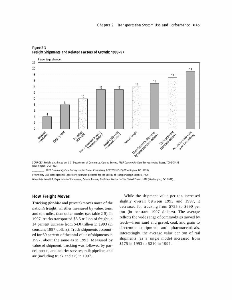
How Freight MovesTrucking (for-hire and private) moves more of thenation’s freight, whether measured by value, tons,and ton-miles, than other modes (see table 2-5). In1997, trucks transported $5.5 trillion of freight, a14 percent increase from $4.8 trillion in 1993 (inconstant 1997 dollars). Truck shipments account-ed for 69 percent of the total value of shipments in1997, about the same as in 1993. Measured byvalue of shipment, trucking was followed by par-cel, postal, and courier services; rail; pipeline; andair (including truck and air) in 1997.
While the shipment value per ton increasedslightly overall between 1993 and 1997, itdecreased for trucking from $755 to $690 perton (in constant 1997 dollars). The averagereflects the wide range of commodities moved bytruck—from sand and gravel, coal, and grain toelectronic equipment and pharmaceuticals.Interestingly, the average value per ton of railshipments (as a single mode) increased from$175 in 1993 to $210 in 1997.
Chapter 2 Transportation System Use and Performance � 45
Reside
nt
popu
lation
Emplo
ymen
t
Ton-m
iles
of fre
ight
Gross D
omes
tic Prod
uct
(cons
tant d
ollars
)
Retail t
rade s
ales
(cons
tant d
ollars
)
Tons
of fre
ight
Manufa
cturer
’s ship
ments
by va
lue (c
onsta
nt do
llars)
Value o
f freig
ht
(cons
tant d
ollars
)
Wholes
ale tra
de sa
les
(cons
tant d
ollars
)
0
2
4
6
8
10
12
14
16
18
20
22
4
8
10
13 1314
15
17
19
SOURCES: Freight data based on: U.S. Department of Commerce, Census Bureau, 1993 Commodity Flow Survey: United States, TC92-CF-52(Washington, DC: 1993)
_________. 1997 Commodity Flow Survey: United States Preliminary, EC97TCF-US(P) (Washington, DC: 1999).
Preliminary Oak Ridge National Laboratory estimates prepared for the Bureau of Transportation Statistics, 1999.
Other data from U.S. Department of Commerce, Census Bureau, Statistical Abstract of the United States: 1998 (Washington, DC: 1998).
Percentage change
Figure 2-3Freight Shipments and Related Factors of Growth: 1993–97

Local vs. Long-Haul FreightFreight shipments can be categorized as local(less than 100 miles), intraregional (between 100and 1,000 miles), and interregional (over 1,000miles).5 In 1997, local shipments constitutednearly 67 percent of the weight (7.7 billion tons),40 percent of the value ($3 trillion), but only 9percent of the ton-miles (254 billion) of all CFSshipments, about the same proportion of thevalue, tons, and ton-miles identified by the CFSin 1993, (see table 2-6).
Intraregional shipments in 1997 accountedfor 45 percent of the value of goods shipments($3.4 trillion), 29 percent of the tons (3.3 billiontons), and 62 percent of the ton-miles (1.7 tril-lion). Interregional shipments accounted for arelatively small proportion of the total CFS ton-
nage (4.4 percent in 1997), but they have had alarge impact on the U.S. transportation systemand the tonnage of such shipments has grownrapidly. In 1997, longer haul shipments account-ed for 29 percent of the CFS ton-miles, about thesame proportion as in 1993. Nevertheless, thetonnage moving such long distances grew about40 percent, with value increasing nearly 30 per-cent in real terms.
Shipments of Major CommoditiesTable 2-7 presents the relative shares of majorcommodities shipped by domestic establishmentsin 1997 as measured by the CFS. The commodi-ties are based on the two-digit StandardClassification of Transported Goods (SCTG)coding system.6 Because data on freight ship-ments in 1993 are not currently available in the
46 � Transportation Statistics Annual Report 1999
Table 2-5Modal Shares of Freight Shipments within the United States by Domestic Establishments: 1993 and 1997
1993R 1997P 1993R 1997P 1993R 1997P
Truck (for-hire, private, both) 71.2 69.4 53.1 58.3 24.4 27.9Rail (includes truck and rail) 5.3 4.8 13.2 11.2 27.5 26.7Water 2.9 2.5 12.2 11.1 23.2 20.4Pipeline 5.0 4.2 15.5 13.7 18.0 17.6Parcel, postal, courier services 9.1 10.9 0.2 0.2 0.4 0.5Air (includes truck and air) 2.2 2.7 0.0 0.0 0.1 0.2Other and unknown modes 4.2 5.6 5.9 5.5 6.5 6.8
Total (domestic plus export shipments) 100.0 100.0 100.0 100.0 100.0 100.0
KEY: P = preliminary; R = revised.
SOURCES: U.S. Department of Transportation, Bureau of Transportation Statistics, based on U.S. Department of Commerce, Census Bureau, 1993Commodity Flow Survey: United States, TC92-CF-52 (Washington, DC: 1995).
____. 1997 Commodity Flow Survey: United States Preliminary, EC97TCF-US(P) (Washington, DC: 1999).
Estimates for crude petroleum shipments by pipelines prepared for the Bureau of Transportation Statistics by Oak Ridge National Laboratory.
Value (percent) Tons (percent) Ton miles (percent)Mode
5Supplementary data are used to estimate total freight ship-ments in 1993 and 1997, but this supplementary data doesnot include freight movement for specific commodities,shipment sizes, and average length of haul per ton of ship-ments. Such changes can only be discussed using CFS dataalone.
6BTS and the Census Bureau are retabulating the 1993 CFSdata from the Standard Transportation CommodityClassification to the SCTG to make the data directly com-parable. These data are expected to be available starting infall 1999.

Chapter 2 Transportation System Use and Performance � 47
Ranked by value
Commodity PercentElectronic and other electrical
equipment and components and office equipment 12.1
Motorized and other vehicles (including parts) 7.8
Textiles, leather, and articles of textiles or leather 7.2
Miscellaneous manufactured products 6.8
Mixed freight 5.9Machinery 5.9Other prepared foodstuffs
and fats and oils 4.6Printed products 4.1Plastics and rubber 3.9Base metal in primary or
semifinished forms and in finished basic shapes 3.8
Ranked by tons
Commodity PercentGravel and crushed stone 16.0Coal and coal products 10.8Gasoline and aviation
turbine fuel 7.8Nonmetallic mineral products 7.6Cereal grains 4.8Logs and other wood in
the rough 4.3Fuel oils 3.9Natural sands 3.9Coal and petroleum
products, n.e.c. 3.8Other prepared foodstuffs
and fats and oils 3.5
Ranked by ton-miles
Commodity PercentCoal and coal products 18.5Cereal grains 8.6Gasoline and aviation
turbine fuel 5.0Other prepared foodstuffs
and fats and oils 4.6Base metal in primary or
semifinished forms and in finished basic shapes 4.6
Basic chemicals 4.2Gravel and crushed stone 3.6Wood products 3.6Nonmetallic mineral products 3.4Pulp, newsprint, paper,
and paperboard 3.3
Table 2-6U.S. Freight Shipments by Distance Shipped: 1993 and 1997(Commodity Flow Survey data only)
Change Change ChangeDistance shipped 1993 1997P (%) 1993 1997P (%) 1993 1997P (%)
Less than 100 miles $2,527 $3,051 20.7 6,490 7,713 18.9 226 254 12.3
100–999 miles 2,981 3,420 14.8 2,833 3,337 17.8 1,492 1,743 16.8
1,000 miles or more 895 1,153 28.8 366 513 40.0 703 812 15.5
Total $6,402 $7,624 19.1 9,688 11,563 19.3 2,421 2,808 16.0
KEY: P = preliminary.
SOURCES: U.S. Department of Commerce, Census Bureau, 1993 Commodity Flow Survey: United States, TC92-CF-52 (Washington, DC: 1995).
____. 1997 Commodity Flow Survey: United States Preliminary, EC97TCF-US(P) (Washington, DC: 1999).
Value(constant $ billions)
Tons(millions)
Ton-miles(billions)
Table 2-7Major Commodities Shipped in the United States: 1997P
(Commodity Flow Survey data only)
KEY: n.e.c. = not elsewhere classified; P = preliminary.
NOTE: Data exclude shipments of crude petroleum.
SOURCES: U.S. Department of Transportation, Bureau of Transportation Statistics, based on U.S. Department of Commerce, Census Bureau, 1993Commodity Flow Survey: United States, TC92-CF-52 (Washington, DC: 1995).
____. 1997 Commodity Flow Survey: United States Preliminary, EC97TCF-US(P) (Washington, DC: 1999).

SCTG, this discussion of commodities coversshipments in 1997 only. Moreover, it must beremembered that the CFS does not cover severalimportant commodities such as crude petroleumpipeline movements.
Merchandise in the category “electronic,other electrical equipment and components, andoffice equipment” accounted for the highest dol-lar value ($925 billion) of CFS shipments in1997, followed by motorized and other vehicles(including parts); textiles, leather, and articles oftextiles and leather; and miscellaneous manufac-tured products.
As for total tonnage shipped, the top com-modity groups were gravel and crushed stone(1.8 billion tons), coal and coal products, gaso-line and aviation fuel, and nonmetallic mineralproducts. Although gravel and crushed stoneaccounted for 16 percent of total CFS tons, ship-ments in this category accounted for less than 1percent of the value and about 4 percent of theton-miles of all shipments, impacting mostlylocal transportation.
The transportation of coal generated the mostton-miles (520 billion), followed by cereal grains,gasoline and aviation fuel, and prepared food-stuffs. Coal produced the most ton-miles because,unlike gravel and stone, which move mostly inlocal areas, coal is often shipped long distances;coal mined in Wyoming and Montana is trans-ported nationwide. In 1997, a ton of coal wasshipped 416 miles on average, compared with 55miles for a ton of gravel and crushed stone.
Shipment SizeIn analyzing CFS data, freight shipments weredivided into several weight categories: less than100 pounds, 100 to 999 pounds, 1,000 to49,999 pounds, and over 50,000 pounds. In1997, the value of CFS shipments under 100pounds exceeded $1.1 trillion, 37 percent greaterthan in 1993 (in real terms) (see table 2-8).
Growth in parcel, postal, and courier servicesand an increase in just-in-time production anddistribution systems are partly responsible forthis rise in smaller size shipments. Shipments ofless than 100 pounds are often high-value, time-sensitive commodities transported by truck andair intermodal combinations, or by truck alone.In 1997, such small-size shipments accounted for15 percent of the value of CFS shipments, littledifferent from the 13 percent in 1993.
Large-size shipments (over 50,000 pounds)accounted for nearly 66 percent of the CFS ton-miles, 56 percent of tons shipped, but only 12 per-cent of the value of shipments in 1997. The relativeshare of large-size shipments fell slightly between1993 and 1997 in value, tons, and ton-miles.
INTERNATIONAL FREIGHT
The importance of international trade to the U.S.economy can be seen in the increased value ofU.S. merchandise trade7 in recent decades.Between 1980 and 1997, the real-dollar value ofU.S. merchandise trade more than tripled, from$496 billion to $1.7 trillion (in chained 1992dollars). In addition, the ratio of the value of U.S.merchandise trade relative to U.S. GDP doubledfrom about 11 percent in 1980 to 23 percent in1997 (USDOC ITA 1998).
During the past two decades, changes can beseen in the geography of trade. Trade with AsianPacific countries grew greatly. In 1997, fiveAsian countries were among the top 10 U.S.trading partners, despite a slight downturn intrade in the second half of 1997 related to eco-nomic problems in the region (see table 2-9).
48 � Transportation Statistics Annual Report 1999
7Unless otherwise noted, the value of U.S. merchandiseimports is based on U.S. general imports, customs valuebasis. Export value is f.a.s. (free alongside ship) and repre-sents the value of exports at the port of exit, including thetransaction price, inland freight, insurance, and othercharges. Generally, data for imports that are valued at lessthan $1,250 and exports that are valued at less than $2,500are excluded.

These five countries accounted for 26 percent ofoverall U.S. trade in 1997, up from 17 percent in1980. Canada and Mexico were the first andthird largest U.S. trading partners in 1980 and in1997. While the rankings remained the same, theU.S. trade relationship with these two countriesdeepened. In 1980, Canada and Mexico together
accounted for 22 percent of all U.S. trade byvalue. By 1997, this had increased to over 30 per-cent (USDOC 1985; USDOC Census FTD 1997).
Changes over the past two decades alsooccurred in the commodities traded. Highervalue manufactured goods now dominate U.S.trade, accounting for $1.3 trillion or 85 percent
Chapter 2 Transportation System Use and Performance � 49
Table 2-8Shipments by Size: 1993 and 1997(Commodity Flow Survey data only)
Change Change ChangeShipment size 1993 1997P (%) 1993 1997P (%) 1993 1997P (%)
Less than 100 pounds 852 1,165 36.6 35 41 17.8 12 15 26.4
100–999 pounds 995 1,215 22.1 139 168 20.1 30 41 37.6
1,000–49,999 pounds 3,735 4,360 16.7 3,830 4,877 27.4 728 903 24.1
Over 50,000 pounds 820 885 7.9 5,685 6,477 13.9 1,651 1,849 12.0
KEY: P = preliminary.
SOURCES: U.S. Department of Transportation, Bureau of Transportation Statistics, based on U.S. Department of Commerce, Census Bureau, 1993Commodity Flow Survey: United States, TC92-CF-52 (Washington, DC: 1995).
____. 1997 Commodity Flow Survey: United States Preliminary, EC97TCF-US(P) (Washington, DC: 1999).
Value(constant $ billions)
Tons(millions)
Ton-miles(billions)
Table 2-9Top 10 U.S. Merchandise Trade Partners by Value: 1980 and 1997 (chained 1997 dollars)
1980
Rank Country Imports Exports Total
1 Canada 77,240 65,942 143,182
2 Japan 57,221 38,732 95,954
3 Mexico 23,437 28,216 51,653
4 West Germany 21,784 20,419 42,203
5 United Kingdom 18,336 23,649 41,985
6 Saudi Arabia 23,564 10,746 34,310
7 France 9,809 13,945 23,754
8 Taiwan 12,769 8,080 20,849
9 Netherlands 3,564 16,151 19,715
10 Venezuela 9,913 8,520 18,433
1997
Rank Country Imports Exports Total
1 Canada 168,201 151,767 319,968
2 Japan 121,663 65,549 187,212
3 Mexico 85,938 71,388 157,326
4 China 62,558 12,862 75,420
5 United Kingdom 32,659 36,425 69,084
6 Germany 43,122 24,458 67,580
7 Taiwan 32,629 20,366 52,995
8 South Korea 23,173 25,046 48,219
9 Singapore 20,075 17,696 37,771
10 France 20,636 15,965 36,601
SOURCE: U.S. Department of Transportation, Bureau of Transportation Statistics, January 1999, based on data from U.S. Department of Commerce,Census Bureau, Statistical Abstract of the United States (Washington, DC: Various years).

of the value of all merchandise trade in 1997.Of these goods, motor vehicles, computers,telecommunications equipment, and aircraft areamong the top U.S. import and export com-modities by value. While the value of manufac-tured goods increased as a share of U.S. trade,the share of agricultural commodities declinedfrom 13 percent in 1980 to 6 percent in 1997.Mineral fuels accounted for approximately 6percent of the value of U.S. trade in 1997, pri-marily imports of crude petroleum and petrole-um products (USDOC ITA 1999).
The relative roles of transportation modes incarrying U.S. international trade have changed inrecent decades, especially in terms of value. Dueto the way in which data on U.S. trade are col-lected, it is not possible to fully calculate the roleof intermodal or multimodal moves of interna-tional freight. Modal shares, therefore, representsingle modes in use at a U.S. port of entry or exit.In 1997, water was the predominant mode inboth value and tonnage, while air accounted fornearly 28 percent of the value but only a smallpart of the tonnage (see figure 2-4). Truck andrail accounted for smaller, but still importantshares.8
Waterborne TradeWhile waterborne trade accounted for morethan three-quarters of the tonnage of U.S. inter-national trade in 1997, its share of the value ofU.S. trade declined from 62 percent in 1980 to40 percent in 19979 (USDOC Census 1994, table1062; USDOC Census FTD 1997). Among thefactors that explain this decline are greater landtrade with Canada and Mexico and the demandfor faster delivery of high-value commodities,which has increased air trade.
In 1997, maritime ports on the west coast ofthe United States accounted for 42 percent of thevalue of U.S. waterborne trade with other coun-tries compared with only 24 percent in 1980.East coast ports’ share by value, however, de-clined from 41 percent to 38 percent over thisperiod (remaining relatively stable in the last 5years), and the share of value for Gulf ports alsodropped from 33 percent to 18 percent (USDOCCensus 1997, table 1069; USDOT MARAD1998). Increased trade with Asian Pacific coun-tries between 1980 and 1997 helps explain thiseast to west coast shift. The financial crisisimpacting several Asian economies, beginning inthe second half of 1997,10 caused a slight de-crease in overall merchandise trade by west coastports. Between 1996 and 1997, the value of totalinternational trade by west coast ports decreased1.5 percent compared with a 0.4 percentdecrease for east coast ports. Because of theappreciation of the U.S. dollar in relation to sev-eral Asian currencies, imports through westcoast ports increased 3 percent between 1996and 1997, while exports declined 12 percent.
The ports of Long Beach and Los Angelesaccount for the majority of west coast water-borne trade. Long Beach is also the leading U.S.port both by value and for containerized trade,as measured by the number of 20-foot equivalentunits (TEUs) handled. In 1997, $85 billionworth of international trade passed through the
50 � Transportation Statistics Annual Report 1999
8BTS estimated the weight of U.S. land exports. (For waterand air, see USDOC Census FTD 1997. Truck, rail, pipeline,and other and unknown are from BTS analyses and Trans-border Surface Freight Data.)
9Excludes waterborne in-transit shipments. In-transit ship-ments are merchandise shipped through the United States intransit from one foreign country to another.10The causes of the Asian financial crisis are complex andmultifaceted. However, a precipitating event occurred inJuly 1997 when the government of Thailand abandoned itsefforts to maintain a fixed exchange rate for its currency, thebaht. The baht quickly depreciated by more than 20 per-cent. Within a few days, most neighboring countries hadalso abandoned their fixed exchange rates. Currency crisesoften have destabilizing effects on international trade. U.S.overall trade with several Asian economies decreased in1997, while the U.S. trade deficit with several Asian coun-tries increased. (For further information, see USITC 1998.)

port of Long Beach, and the port handled 2.7 mil-lion TEUs (see table 2-10). Other west coast portssuch as Los Angeles, Seattle, and Tacoma are alsoimportant gateways for U.S. trade with Asia.11
The port of New York/New Jersey is the eastcoast leader in both the value of trade ($68 bil-lion) and in the number of containers (1.7 millionTEUs) handled in 1997. Charleston and Norfolkare also major east coast container ports. Theimportance of Gulf ports (e.g., Houston andSouth Louisiana) in the trade of bulk commodi-ties and crude petroleum can be seen from theirlisting as the top two U.S. ports by tonnage.
Air FreightAir freight moves both by all-cargo carriers and car-riers that transport passengers. Between 1980 and1997, air freight’s share of the value of U.S. inter-national merchandise trade increased from 16 per-
cent to nearly 28 percent. Commodities that moveby air tend to be high in value; air’s share of U.S.trade by weight was less than 1 percent in 1997.
Western European and Asian Pacific countriesdominate air freight to and from the United States.The top three countries by value of air freight withthe United States are Japan, the United Kingdom,and Singapore. New York’s John F. Kennedy(JFK) International Airport was the leading gate-way for shipments into and out of the UnitedStates by all modes, accounting for over $89 bil-lion in 1997. Following JFK were the airports ofChicago, Los Angeles, and San Francisco.12
North American Merchandise TradeU.S. merchandise trade with Canada andMexico represents 30 percent of all U.S. interna-tional trade, with Canada accounting forapproximately 20 percent and Mexico 10 percent.U.S. trade with Mexico has grown more quicklythan with Canada, and in 1997 Mexico surpassedJapan as the second largest market for U.S. mer-
Chapter 2 Transportation System Use and Performance � 51
Water Air Truck Rail Pipeline Other andunknown
0
5
10
15
20
25
30
35
4040.2
27.8
20.8
4.50.9
5.9
45
SOURCE: U.S. Department of Transportation, Bureau of Transportation Statistics, January 1999, except water and air data from U.S. Department of Commerce, Census Bureau, Foreign Trade Division.
Percent
Value
Figure 2-4Modal Shares of U.S. Merchandise Trade by Value and Tons: 1997
Water Air Truck Rail Pipeline Other andunknown
Percent
Tons
0
10
20
30
40
50
60
70
80
90
77.0
0.4
11.95.7 5.0 4.9
11Many individual west coast ports were also impacted bythe Asian financial crisis. The overall value of the port ofLong Beach’s international trade declined 2 percent between1996 and 1997. The decline in Long Beach’s export tradewas more dramatic, 18 percent. The ports of Seattle andOakland also saw notable decreases in export trafficbetween 1996 and 1997.
12San Francisco includes the San Francisco InternationalAirport and other smaller regional airports. Chicago includesO’Hare, Midway, and other smaller regional airports.

chandise exports (although Mexico remained thethird largest trading partner overall). Between1993 and 1997, trade with North American FreeTrade Agreement (NAFTA)13 partners increased62 percent in current dollars, from $293 billionto $475 billion. During this same period, U.S.trade with Mexico grew most rapidly, almostdoubling from $81 billion in 1993 to $157 bil-lion in 1997 (USDOC 1998, table 1323;USDOC Census FTD 1997).
In terms of commodities, motor vehicles andmotor vehicle parts and accessories dominate tradebetween all of the North American countries.Other leading North American trade commoditiesinclude consumer electronics, telecommunicationsequipment, and aircraft equipment and parts. Inaddition, crude petroleum, natural gas, and petro-leum products are important U.S. imports fromboth Canada and Mexico. Mexico is also a chiefsource of U.S. imports of clothing and textiles,while paper products, furniture, and wood prod-ucts are among leading U.S. imports from Canada.
Truck trade represented almost 70 percent ofthe value and 33 percent of the tonnage of overallNAFTA merchandise trade in 1997.14 Rail’s sharewas approximately 15 percent both by value andweight. Rail played a greater role in U.S.-Canadiantrade than in U.S.-Mexican freight movement. Tenstates accounted for approximately two-thirds ofthe value of North American land trade in 1997.15
These were Michigan, Texas, California, NewYork, Ohio, Illinois, Pennsylvania, Indiana, NorthCarolina, and Tennessee. Many of these states con-tain major population and manufacturing centers.
52 � Transportation Statistics Annual Report 1999
Table 2-10Top Water Ports for International Trade: 1997
By 20 foot equivalent units (TEUs)
Rank Port name TEUs
1 Long Beach, CA 2,673,1992 Los Angeles, CA 2,084,9243 New York,NY/NJ 1,738,3914 Charleston, SC 955,4885 Seattle, WA 953,3046 Oakland, CA 843,0667 Norfolk, VA 769,7188 Miami, FL 623,6589 Houston, TX 609,451
10 Tacoma, WA 551,164
By value (billions of current U.S. dollars)
Rank Port name Value
1 Long Beach, CA 85.32 Los Angeles, CA 73.43 New York, NY and NJ 68.04 Houston, TX 37.15 Seattle, WA 33.66 Charleston, SC 27.37 Oakland, CA 25.48 Norfolk, VA 25.09 Tacoma, WA 19.6
10 Baltimore, MD 18.8
By tonnage (millions of U.S. short tons)
Rank Port name Tonnage
1 Houston, TX 102.82 South Louisiana, LA 76.83 Corpus Christi, TX 62.24 New York, NY and NJ 56.75 New Orleans, LA 52.46 Baton Rouge, LA 38.47 Long Beach, CA 38.48 Texas City, TX 37.49 Norfolk, VA 35.4
10 Beaumont, TX 33.6
NOTES: Value data do not include in-transit shipments. Tonnagedata, unlike port tonnage data for previous years, do not include in-transit shipments.
SOURCES: TEU data: U.S. Department of Transportation, MaritimeAdministration, Office of Statistical and Economic Policy, based ondata from the Journal of Commerce, Port Import and ExportReporting System (PIERS).Value data: U.S. Department of Transportation, MaritimeAdministration, Office of Statistical and Economic Policy, AnnualWaterborne Databanks 1996, 1998.Tonnage data: U.S. Army Corps of Engineers, Navigation DataCenter, special tabulation, December 1998.
13The United States, Canada, and Mexico signed the agree-ment in December 1993 and the treaty entered into force onJanuary 1, 1994.14BTS estimate.15Top origin and destination states are based on U.S. inter-national trade data collected from administrative records.Due to filing requirements and procedures, border stateactivity may be overrepresented. In addition, trade data donot always reflect physical transportation flows. The loca-tion is often misrepresented because trade documents are notalways filed where shipments physically cross the border.
On the U.S.-Canadian border, 10 gatewaysaccounted for approximately 83 percent offreight moved by trade, while for U.S.-Mexicantrade, the top 10 land gateways account for 93percent. The three largest gateways for U.S.-Canadian land trade were Detroit, Buffalo-Niagara Falls, and Port Huron (see figure 2-5).On the U.S.-Mexican border, the top gatewaywas Laredo, followed by El Paso, and OtayMesa, California. Truck traffic accounted for themajority of the trade at most of these gateways.Port Huron, Michigan, and Eagle Pass, Texas,were important rail gateways. For many of thesegateways, the shipment origins and destinationswere outside the state in which the gateway islocated. For example, nearly four-fifths of theshipments that crossed the border at Laredo hadtheir origins or destinations outside of Texas.Three-quarters of the shipments that crossed theborder at Buffalo have their origins or destina-tions outside of New York (USDOT BTS 1998b).
Although much North American trade takesplace between bordering states or provinces suchas Ontario and Michigan and Texas andChihuahua, other trade flows are characterizedby longer distances (e.g., truck shipmentsbetween California or Texas and Ontario forU.S.-Canadian trade and between Texas andJalisco and Michigan and the Mexico City met-ropolitan area for U.S.-Mexican trade). Ship-ments from maquiladora16 plants and facilitiesalong the U.S.-Mexican border accounted forsome of the shorter flows in U.S.-Mexican trade,while some of the longer flows were betweenmotor vehicle manufacturing and productioncenters at diverse locations in Mexico, the UnitedStates, and Canada.
A Multimodal ViewAir, land, and water modes are all important intransporting goods in U.S. international trade.Figure 2-6 illustrates the top ports of entry andexit for U.S. international trade shipments byvalue in 1997. The leading gateway overall in1997 was JFK International Airport in New Yorkwith $89 billion of activity. This was followed bythe water port of Long Beach, California, whichhandled $85 billion worth of shipments, andDetroit, Michigan, a land gateway with $83 bil-lion worth of shipments in 1997. Changes in themix of commodities traded internationally, geo-graphic shifts in centers of production, globaltrade patterns, and many other factors will con-tinue to affect these gateways as well as the move-ment of international trade shipments to, from,and within the United States.
USE AND PERFORMANCE
Many factors affect the performance of thetransportation system: accessibility, safety, envi-ronmental restraints, input costs, energy efficien-cy, capacity-to-demand ratios, reliability, traveltime and delay, goods damage, and a host ofother variables. Safety, energy efficiency, envi-ronmental impacts, and economic measures ofthe system’s performance are discussed elsewherein this report. The following section focuses ontrends in the use of the transportation systemand how well the transportation system deliversservices that people and businesses want, such asspeed, reliability, security, convenience, and com-fort, when they buy a passenger ticket, forwarda shipment, or travel during peak hours. Thus,the discussion of performance that follows high-lights such indicators as: 1) on-time perfor-mance, congestion, and delay; 2) the security ofgoods during shipment against damage or loss;3) productivity; and 4) accessibility of transit ser-vices to persons with physical disabilities. In
Chapter 2 Transportation System Use and Performance � 53
16Maquiladoras are manufacturing or assembly plants locat-ed in Mexico that provide parts, components, and addition-al processing for manufactured products produced by U.S.or multinational companies. Maquiladora plants locatednear the U.S. border are often wholly owned or are a sub-sidiary of a U.S. or multinational company.

addition, selected operational efficiency indica-tors will be discussed for some modes.
HighwayVehicle-miles traveled (vmt) on public roadsincreased 68 percent between 1980 and 1997,with urban vmt growth outpacing rural vmt—83percent to 49 percent. Some of the growth in urbanareas is due to the expansion of urban boundariesand urban population (USDOT FHWA variousyears) (see table 2-11). Urban Interstate travelincreased the most over these years, about 4.9 per-cent annually, although other urban arterials stillcarried the most traffic in 1997.
For the highway user, traffic congestion anddelay are measures of highway performance.Unfortunately, direct measures are not nowavailable to determine whether congestion anddelay are getting better or worse for the nation asa whole. Two indirect methods are used, howev-er: 1) congestion and delay calculations based ondaily volume-to-capacity ratios such as thosefound in the Federal Highway Administration’s(FHWA’s) Highway Performance MonitoringSystem (HPMS); and 2) trip speed estimatesbased on commuter trip length and travel timedata collected from travel surveys.
54 � Transportation Statistics Annual Report 1999
Value of freight entering and exiting ports(US $ billions)
75,000
37,500
18,750
ExportsImports
Blaine
SweetgrassPortal Pembina
Highgate Springs–Alburg
Champlain–Rouses Point
Port Huron
Alexandria Bay
Buffalo–Niagara Falls
Detroit
Del Rio
Eagle Pass
El Paso
Otay Mesa Station
Calexico
Calexico–EastNogales
Laredo
Hidalgo
Brownsville-Cameron
Figure 2-5Top Border Land Ports: 1997
NOTES: Data include transshipments between the United States and Mexico. Trade levels reflect the mode of transportation as a shipment entered or exited a U.S. Customs port. Alaska is not shown as its border land ports do not fit the criteria for inclusion in this figure.
SOURCE: U.S. Department of Transportation, Bureau of Transportation Statistics, Transborder Surface Freight Data, 1998.

Two estimates of congestion using volume-to-capacity ratios are discussed here: the TexasTransportation Institute’s (TTI’s) studies ofurban congestion and FHWA’s estimates of vol-ume-to-service-flow (where service flow is ameasure of capacity). In addition, results fromvarious Nationwide Personal TransportationSurveys augment these estimates. As shownbelow, the congestion indicators developed bythese indirect methods often produce conflictingviews about traffic congestion and/or delay.
TTI’s most recent analysis of urban highwaycongestion shows highway congestion and traf-fic delay rising in the United States.17 Of the 70
urban areas included in the TTI study, the esti-mated level of congestion declined in only 2—Phoenix and Houston—between 1982 and1996. Congestion in most other urban areasincreased, dramatically in some instances. Thenumber of urban areas in the study experiencingunacceptable congestion rose from 10 of the 70in 1982 to 39 in 1996, with the average roadwaycongestion index—measured by travel volumeper road lane—rising about 25 percent from0.91 to 1.14. TTI selected an index of 1.00 orgreater as the threshold for unacceptable conges-tion (see figure 2-7).
Chapter 2 Transportation System Use and Performance � 55
Value of freight enteringand exiting gateways($ billions)
100
50
25
ExportsImports
Port of Seattle
Port of Blaine
Port of Tacoma
Port of Sweetgrass
Port of Portland
Port of Oakland
Los AngelesInternational Airport
San Francisco International Airport
Port of Long Beach
Port of Otay Mesa
Port of Nogales
Port of Eagle Pass
Houston InternationalAirport
Port of Laredo
Dallas-Ft. Worth International Airport
Anchorage
Port of Hidalgo
Port of Brownsville-Cameron
Port of Corpus Christi
Port of El Paso
Port of Los Angeles
Port of Portal Port of Pembina
Port of South Louisiana
Port of Houston
Miami InternationalAirport
Port of Miami
Port of Port Everglades
New OrleansPort of Baton Rouge
Port of New Orleans
Chicago O’HareInternationalAirport
Atlanta
Port of Norfolk
Port of New York
Air
Legend
Water
Land
Boston Logan Airport
Port of Champlain-Rouses Pt.
Port of Alexandria Bay
Port of Buffalo-Niagara Falls
Port of Port Huron
Port of Detroit
Cleveland InternationalAirport
Newark InternationalAirport
Port of Philadelphia
JFK InternationalAirport
Port of Jacksonville
Port of Savannah
Port of Charleston
Port of Baltimore
NOTES: Air—Values for some airports may include a low level (generally less than 2 percent of the total value) of small user-fee airports located in the same regional area. In addition, due to the Census Bureau’s confidentiality regulations, data for nearby individual courier operations (e.g., DHL, Federal Express, United Parcel Service) are included in the airport totals for New York Kennedy, New Orleans, Los Angeles, Cleveland, Chicago O’Hare, Miami, and Anchorage. Land—Data include transshipments between the United States and Mexico. Trade levels reflect the mode of transportation as a shipment entered or exited a U.S. Customs port. Includestruck, rail, pipeline, and other modes of land transportation.
SOURCES: Air—U.S. Department of Commerce, Census Bureau, Foreign Trade Division, special tabulation. Maritime and Great Lakes—U.S. Department of Transportation, Maritime Administration, Office of Statistical and Economic Policy, U.S. Waterborne Exports and General Imports, Annual 1997 (Washington, DC: 1998). Land—U.S. Department of Transportation, Bureau of Transportation Statistics, Transborder Surface Freight Data, 1998.
Figure 2-6Top Freight Gateways by Shipment Value: 1997
17 The primary data source used by TTI is the HPMS.

Table 2-12 presents an index of roadway con-gestion, annual delay, and wasted fuel. In 1996,drivers in the 70 study areas experienced an aver-age of 40 hours of delay each over the course ofthe year—the equivalent of a full work week.This was 8 percent more delay than in 1990, and150 percent more than in 1982 when the averagewas 16 hours. In 1982, peak-hour travel took 13percent more time than travel in less congestedconditions (for the same distance traveled). By1996, peak period travel required 25 percentmore travel time on average, and in some cities ittook nearly 50 percent more time than offpeaktravel (TTI 1998).
TTI estimated that the total annual costs ofcongestion in the 70 areas reached $74 billion in1996, $65 billion due to delay (productivity loss)and $9 billion due to wasted fuel. Costs rangedfrom $333 per driver in smaller cities to $936 inlarge cities, averaging about $629 overall. Thestudy estimated that 6.7 billion gallons of fuelwas wasted in these areas due to traffic conges-
tion, compared with about 2.7 billion gallons in1982 (TTI 1998).
FHWA’s volume-to-capacity estimates onlypartly confirm TTI’s findings, though changes inthe definition of congestion in 1995 make a fullcomparison difficult. Moreover, FHWA’s dataonly measure recurring congestion, which occursduring normal daily operations because demandexceeds capacity, while TTI’s data also measurenonrecurring congestion, which occurs as aresult of traffic crashes, breakdowns, or otherirregular incidents. FHWA’s 1995 through 1997estimates show slight increases in congestion forprincipal arterials (i.e., arterials other thanInterstates, freeways, and expressways). UrbanInterstates, on the other hand, show a reductionin delay over the period. Similarly, urban free-ways and expressways show a decrease since1995. Rural roads show no noticeable increase(USDOT FHWA Various years, table HM-61).
Commuter speeds, as measured by the NPTSin 1983 and 1995, show a 20 percent increasefrom 28 mph to 34 mph (USDOT FHWA1997c, 13). At first glance, the NPTS data mightseem to contradict the TTI findings. There
56 � Transportation Statistics Annual Report 1999
Table 2-11Highway Vehicle-Miles Traveled byFunctional Class: 1980–97 (millions)
Percentage1980 1997 change
UrbanInterstate 161,242 351,371 124.1Other arterials 484,189 846,596 74.8Collectors 83,043 130,461 57.1Local 126,791 222,024 75.1
Total 855,265 1,560,452 82.5
RuralInterstate 135,084 240,121 77.8Other arterials 262,774 391,481 49.0Collectors 189,468 253,807 34.0Local 84,704 114,511 35.2
Total 672,030 999,920 48.8
Total 1,527,295 2,560,372 67.6
SOURCE: U.S. Department of Transportation, Federal HighwayAdministration, Highway Statistics (Washington, DC: Various years).
1982 1990 1996
100
90
80
70
60
50
40
30
20
10
0
Uncongested
Moderate
Heavy
Severe
SOURCE: Texas Transportation Institute, Urban Roadway Congestion AnnualReport: 1998 (College Station, TX: 1998), p. 35.
Percentage of person-miles of travel
Figure 2-7Congested Person-Miles of Travel in 70 Urban Areas

are several plausible reasons for different find-ings, however. First, TTI only includes urbanareas, while the NPTS also includes non-urbanareas, where congestion is typically less severe ornonexistent. Second, the NPTS data includecommuting by all modes, while TTI onlyincludes highway modes of travel. Thus, theNPTS results reflect commuter decisions in the1980s and 1990s to switch from car pools andtransit to single-occupant vehicle trips, whichoften save time for the individual workers, butincrease road congestion. Other reasons com-mute speeds may have increased are metropoli-tan decentralization (people have moved toplaces where speeds are higher) and the wideningof the peak period because of work-time flexibil-ity (USDOT FHWA 1997c).
In 1995, the NPTS for the first time includedcustomer satisfaction questions that are helpfulin judging how well the transportation systemmeets people’s expectations. Nearly half ofrespondents said that congestion was no prob-lem at all, with about one-third saying it was asmall problem and 20 percent saying it was alarge problem. About one-quarter of people inurban and suburban areas reported that conges-tion was a large problem, whereas 37 percent ofsuburban residents and 29 percent of urban res-
idents reported it as a small problem. Ruralrespondents report the least problem with con-gestion and town and second-city18 residents fallsomewhere in between. A question was alsoasked about pavement quality on major high-ways. One-quarter of respondents reported thatit is a large problem, and another 39 percent saidit is a small problem. About 15 percent ofrespondents reported that poor walkways orsidewalks were a large problem in their commu-nity; another 28 percent reported it as a smallproblem; the remaining 57 percent reported itwas no problem (USDOT FHWA 1999a).
AirEnplanements (both domestic and international)increased from 302 million in 1980 to 575 mil-lion in 1997 (USDOT BTS 1998a). The changein enplanements at major hubs can be seen in fig-ure 2-8. Revenue passenger-miles increased from268 billion miles in 1980 to 622 billion miles in1997 (USDOT BTS In press).
Several measures are available to examine theperformance of commercial air travel. Theseinclude on-time information, speed, and baggageand boarding problems.
Chapter 2 Transportation System Use and Performance � 57
Table 2-12Urban Congestion Indicators for 70 Urban Areas: Selected Years
Average Annual delay Wasted fuel Annual fuelroadway congestion per eligible driver per eligible wasted per urban
Year index (person-hours) driver (gallons) area (million gallons)
1982 0.91 16 23 391986 1.01 22 32 541990 1.07 27 39 681992 1.09 30 44 761994 1.11 35 51 841995 1.12 37 54 911996 1.14 40 58 96
SOURCE: Texas Transportation Institute, Urban Roadway Congestion Annual Report: 1998 (College Station, TX: 1998), pp. 11–21.
18 For the definition of second cities, see footnote 3.

In 1997, 78 percent of major carrier flightsarrived on time.19 Although arrival on-time perfor-mance in 1997 was slightly lower than other yearsduring the past decade, it was the first year since1991 that it improved (USDOT Various years).
Throughout the 1990s, aircraft speed ofscheduled large certificated air carrier flights (notincluding small certificated and commuter air-lines) averaged just under 220 mph. Averagespeed is measured as the ratio of flight length toflight duration. Flight length is measured fromairport to airport and does not include any addi-tional mileage due to flight deviations (e.g., goingaround bad weather or circling because of air-port airspace congestion). Flight duration is mea-
sured from departure gate to arrival gate. Thus,this metric measures overall trip speed ratherthan air-over-ground speed.
Both mishandled baggage and complaint rateswere lower in 1997 than they were in 1990,although complaints edged up in 1996 and 1997.Mishandled baggage per 1,000 enplanementswas 4.96 in 1997, compared with 6.73 in 1990.Approximately 2.3 million claims were filed in1997 (USDOT BTS 1998, tables 1-44–1-46).
The number of consumer complaints againstmajor air carriers received by the U.S.Department of Transportation increased in 1997for the second year in a row after several years ofdecline. In 1997, 86 out of every 1 million per-sons enplaned on a major airline registered acomplaint with DOT, the highest rate since 1993(USDOT Various issues).
58 � Transportation Statistics Annual Report 1999
Enplanements(millions)
30
15
7.5
19871997
SOURCE: U.S. Department of Transportation, Bureau of Transportation Statistics, Office of Airline Information, Airport Activity Statistics of Certificated Air Carriers: Summary Tables; Twelve Months Ending December 31,1997 (Washington, DC: 1997).
Seattle
Portland
Denver
Salt Lake City
Las Vegas
Phoenix
San Francisco
Honolulu
San Diego
Los Angeles
Dallas-Fort Worth
Houston
Atlanta
CharlotteWashington
Baltimore
Philadelphia
Newark
BostonNew York
PittsburghDetroit
Chicago
St. Louis
Minneapolis-St. Paul
Cincinnati
Tampa
Miami-Ft. Lauderdale
Orlando
Figure 2-8Enplanements at Major Hubs: 1987 and 1997
19 An aircraft departure or arrival is considered on-time if ittakes place within 15 minutes of its scheduled time.

The percentage of passengers denied boarding(i.e., “bumped” from flights because seats wereoversold by the airline) on the 10 largest U.S. aircarriers has risen appreciably since 1993, from683,000 to 1.1 million passengers in 1997 (from0.15 percent to 0.21 percent of boardings). Volun-tary denials20 made up 95 percent of all denials in1997 and is where virtually all the increase hasbeen concentrated (USDOT Various years).
WaterIn 1997, 2.3 billion tons of cargo were moved bywater, with just over half of it foreign trade.Since 1988, foreign trade tonnage has increasedby 25 percent while domestic freight moved bywater remained about the same at around 1.1billion tons. In 1997, 57 percent of domestic tonsmoved on the inland waterways, 24 percentmoved coastwise, and 11 percent moved lake-wise (the rest was local and intraterritorial traf-fic). Lakewise and inland waterway movementincreased by 13 percent and 7 percent, respec-tively, over this period, while coastwise move-ment declined by 19 percent (USACE 1998).
Port performance is typically measured byannual cargo throughput. In 1997, 150 ports han-dled more than 1 million tons of cargo, and 31ports handled over 10 million tons (see figure 2-9).
The U.S. Army Corps of Engineers providesdata on lock performance, including averageprocessing time, lock closure, and lock traffic,for each lock chamber of the inland waterwaysystem in its Performance Monitoring System(USACE 1999), but no national summary is cur-rently available.
TransitTransit ridership, which is concentrated in a fewlarge metropolitan areas (see figure 2-10),
remained constant between 1987 and 1997 withunlinked trips going from 7.85 million trips in1987 to 7.98 million in 1997, while miles trav-eled increased from about 36 billion to 40 bil-lion. Although bus and heavy-rail ridershipstagnated during this period, it still carried themajority of transit users (see table 2-13). Rider-ship on other modes of transit—especiallydemand responsive service,21 light rail, and fer-ries—markedly increased.
The performance of transit service in theUnited States seems to be improving, at least forfederally subsidized transit for which data areavailable. Vehicle revenue-miles measure theavailability of transit service. From 1987 to1997, total revenue-miles increased 25 percentfrom 2.28 billion miles to 2.85 billion miles.Demand responsive transit revenue-miles tripledfrom 113 million to 350 million. Rail service alsoincreased, with light-rail revenue-miles morethan doubling, commuter rail up 35 percent, andheavy rail up 14 percent (see table 2-13). Bus rev-enue-miles increased only 8 percent but stillaccounted for 56 percent of all vehicle revenue-miles. In general, increases in vehicle revenue-mileage are due to expansion in the geographiccoverage for transit, not increased frequency ofexisting services (USDOT FTA 1999).
The percentage of transit vehicles providingaccessible service under the Americans withDisabilities Act (ADA) varied dramatically bytype of transit, but was generally higher in 1997than in 1993. About 68 percent of buses wereADA accessible in 1997, up from 53 percent in1993. Only 29 percent of commuter rail vehicleswere accessible in 1997, but this was higher thanthe 18 percent in 1993. A relatively large per-centage of heavy-rail vehicles are ADA accessi-
Chapter 2 Transportation System Use and Performance � 59
20 In this type of denial, a customer voluntarily gives uphis/her reserved seat on an overbooked flight, usually inreturn for some form of compensation from the airline.
21 Demand responsive service includes passenger cars, vans,or buses with fewer than 25 seats operating in response tocalls from passengers or their agents rather than on fixedroutes. These include paratransit and dial-a-ride services,but exclude jitneys and other fixed-route services.

60 � Transportation Statistics Annual Report 1999
8
Tonnage(millions)
500
250125
DomesticImportsExports
Figure 2-9Tonnage Handled by Major Water Ports: 1997
NOTE: Major ports were defined as having one port with over 10 million tons shipped in 1997, and were combined with other ports in the same major waterway or located in the same metropolitan statistical area with at least 1 million tons shipped.
SOURCE: U.S. Army Corps of Engineers, Water Resources Support Center, Navigation Data Center, Alexandria, VA.
1
30
11
31
21
39
16
12
1720 26
23
37
19
33
7
25
3
132
27
10
38
36
22
189
14
6
29
15
5
28
24
343235
4
1 Anacortes, WA 2 Ashtabula
Ashtabula, OHConneaut, OH
3 Baltimore, MD 4 Beaumont-Port Arthur
Beaumont, TXPort Arthur, TX
5 BostonBoston, MASalem, MA
6 Calcite, MI 7 Charleston, SC 8 Chicago-Gary
Chicago, ILGary, INIndiana Harbor, INBurns Waterway Harbor, INBuffington, IN
9 Cincinnati, OH
10 Cleveland-LorainCleveland, OHLorain, OHFairport Harbor, OH
11 Columbia RiverPortland, ORVancouver, WALongview, WAKalama, WA
12 Corpus Christi, TX13 Delaware River
New Castle, DEWilmington, DEMarcus Hook, DEChester, PAPaulsboro, NJPhiladelphia, PACamden-Gloucester, NJ
14 DetroitDetroit, MISt. Clair, MIMarine City, MIMonroe, MI
15 Duluth-Superior, MN and WI16 Honolulu, HI17 Houston-Galveston
Houston, TXGalveston, TXTexas City, TXFreeport, TX
18 Huntington, IN19 Jacksonville, FL20 Lake Charles, LA21 Los Angeles-Long Beach, CA22 Memphis, TN23 Mobile, AL24 New York-New Jersey25 Norfolk-Newport News
Norfolk, VANewport News, VA
26 Pascagoula, MS27 Pittsburgh, PA28 Portland, ME29 Presque Isle, MI
30 Puget SoundSeattle, WATacoma, WAEverett, WAOlympia, WA
31 San Francisco BaySan Francisco, CAOakland, CARichmond, CA
32 San Juan, PR33 Savannah, GA34 South Florida
Miami, FLPort Everglades, FL
35 South LouisianaPort of South LouisianaNew Orleans, LABaton Rouge, LAPlaquemine, LA
36 St. Louis, MO37 Tampa, FL38 Toledo, OH39 Valdez, AK

ble—78 percent in 1997—but there has been noimprovement since 1994 (see figure 2-11).
Transit speeds varied greatly in 1997, fromcommuter rail at 33.8 mph—the fastest—to bus,which at 12.9 mph was the slowest. Heavy railwas the second fastest with an average speed of20.7 mph, followed by demand responsive vehi-cles (14.7 mph), and light rail (15.5) (USDOTFTA 1999).
Property damaged during transit operations isanother performance measure. In 1997, directlyoperated transit was responsible for $55.7 mil-lion in property damage, and purchased trans-portation service was responsible for another $5
million.22 This totals $1.39 per 1,000 revenuepassenger-miles in 1997, about the same as in1993, when accounting for inflation (USDOTFTA 1999).
RailRevenue ton-miles reached 1,349 billion in1997, an increase of 47 percent since 1980,although revenue-ton miles increased only 16percent in the eastern United States, but climbed
Chapter 2 Transportation System Use and Performance � 61
Transit passenger-miles(billions)
15
7.5
3.75
BusCommuter rail
Other railOther
NOTE: Large transit markets are defined as having more than 200 million transit passenger-miles. Alaska has no large transit markets, so it is not shown.
SOURCE: U.S. Department of Transportation, Federal Transit Administration, National Transit Database, 1997.
Figure 2-10Largest Transit Markets: 1997
Seattle
Portland
San Francisco
San Jose
Los Angeles
San Diego
Honolulu
Dallas-Ft. Worth
Houston
Puerto Rico Miami
Atlanta
Washington
Baltimore New York-New Jersey
St. Louis
Chicago
Detroit
ClevelandPittsburgh
Philadelphia
BostonMinneapolis
Denver
22 A transit agency may provide transit service itself (direct-ly operated service) or contract with another public or pri-vate entity (purchased transportation).

to 68 percent in the western United States (AAR1998, 61). Figure 2-12 illustrates the geographyof rail tonnage.
Figure 2-13 shows that intermodal (trailer orcontainer on flatcar) and coal are the largest cat-egories of rail traffic, each accounting forapproximately one-quarter of the carloadings ofthe railroad industry. Intermodal trafficincreased from 3.1 million loadings in 1980 to8.7 million in 1997 (AAR 1998). The introduc-tion of doublestack container trains in the early1980s played a major role in this growth. Sincethe late 1970s, when the Powder River Basinopened in Wyoming, coal shipments grew from4.4 million carloads in 1978 to 6.7 million car-loads in 1997, reflecting the increased demandfor low sulfur western coal by electric utilities tocomply with clean air standards (AAR 1980;1998). A combination of chemicals, motor vehi-cles and equipment, and farm products accountfor roughly 20 percent of rail traffic.
Table 2-14 presents 1997’s top 10 state-to-state rail freight flows, as well as the major com-modities handled for these flows. These 10 flowsaccounted for 17 percent of all rail carloads and15 percent of all rail tonnage. Miscellaneous
mixed shipments (i.e., intermodal traffic), whichaccounted for 67 percent of all rail intermodaltraffic, and coal are the major commodities for 7of these 10 flows. The largest rail intermodalflows in the United States were betweenCalifornia and Illinois predominantly represent-ing the U.S. land portion of U.S. exports to andimports from Asia’s Pacific Rim countries. Thelargest coal flows originated in the Powder RiverBasin and terminated at electric power generat-ing plants in Illinois, Texas, and Missouri.
Freight rates (freight revenue per ton-mile)adjusted for inflation declined 2 percent per yearbetween 1993 and 1997, and 1 to 2 percent peryear since the passage of the Staggers Act in1980, compared with an increase of nearly 3 per-cent per year between 1975 and 1980.23 From1993 to 1997, the Class I freight railroads aver-aged an 8 percent return on their net investment,up from an average of 2 percent in the 1970s24
(AAR Various years).
62 � Transportation Statistics Annual Report 1999
Table 2-13Urban Transit Indicators: 1987 and 1997 (thousands)
Change Change Change1987 1997 (%) 1987 1997 (%) 1987 1997 (%)
Demand responsive 113,100 350,076 210 176,800 531,078 200 28,800 88,203 206
Bus 1,484,334 1,605,721 8 17,094,900 17,509,219 2 4,794,300 4,602,031 –4
Commuter rail 169,901 229,608 35 6,806,300 8,037,486 18 311,000 357,199 15
Heavy rail 473,921 539,670 14 11,198,000 12,056,068 8 2,402,100 2,429,455 1
Light rail 18,015 39,802 121 404,400 1,023,708 153 131,300 259,404 98
Ferryboat 1,559 2,015 29 114,100 254,219 123 18,800 42,048 124
Total 2,281,275 2,853,330 25 36,102,300 40,180,219 11 7,847,900 7,982,371 2
SOURCE: U.S. Department of Transportation, Federal Transit Administration, National Transit Database, 1987, 1997 (Washington, DC: 1989, 1999).
Revenue vehicle-miles Passenger miles Ridership (unlinked trips)
23 Calculated using the Bureau of Labor Statistics’ ProducerPrice Index for Line-Haul Operating Railroads (SIC 4011).24 In 1997, Class I railroads had operating revenues of$256.4 million or more.
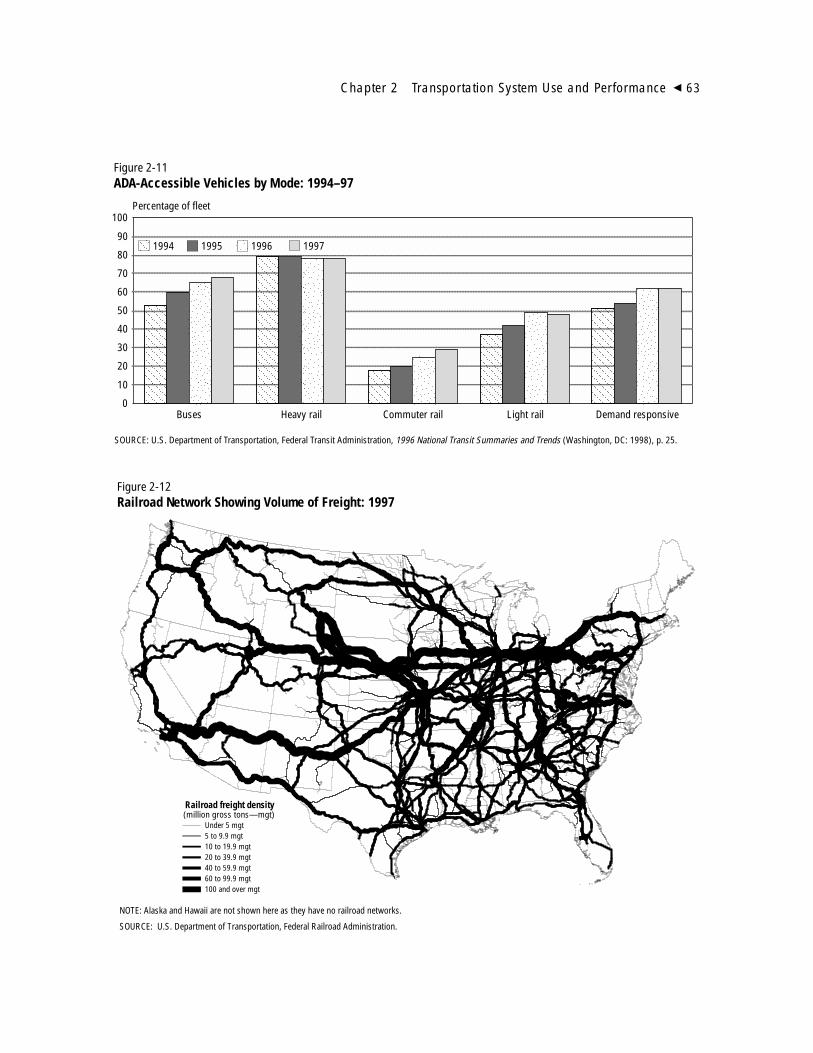
Chapter 2 Transportation System Use and Performance � 63
Buses Heavy rail Commuter rail Light rail Demand responsive0
10
20
30
40
50
60
70
80
90
100
1994 1995 1996 1997
SOURCE: U.S. Department of Transportation, Federal Transit Administration, 1996 National Transit Summaries and Trends (Washington, DC: 1998), p. 25.
Percentage of fleet
Figure 2-11ADA-Accessible Vehicles by Mode: 1994–97
Railroad freight density(million gross tons—mgt)
Under 5 mgt5 to 9.9 mgt10 to 19.9 mgt20 to 39.9 mgt40 to 59.9 mgt60 to 99.9 mgt100 and over mgt
NOTE: Alaska and Hawaii are not shown here as they have no railroad networks.
SOURCE: U.S. Department of Transportation, Federal Railroad Administration.
Figure 2-12Railroad Network Showing Volume of Freight: 1997

Railroad labor productivity grew from 4.2million revenue ton-miles per employee in 1988to 7.6 in 1997 (USDOT BTS 1998a). Because ofrailroad mergers over the past few years, crewsare smaller and fewer freight interchanges
between railroads are necessary. Revenue ton-miles increased due to more frequent and heav-ier traffic moving longer distances.
The value of goods damaged in 1997 was$113 million. Although the total damage donehas increased from the late 1980s, the rate hasdeclined 40 percent from $142 per million ton-miles in 1988 to $84 in 1997 (AAR 1980; 1998).
While freight rail traffic increased, passengerrail traffic remained relatively constant. Therewere 20.2 million Amtrak passengers in fiscalyear (FY) 1997, about the same number as in FY1987. Amtrak’s passenger load factor, however,has declined over the past decade, decreasingfrom 53 percent in 1988 to 47 percent in 1997(NRPC 1996; 1999).
Amtrak operated approximately 22,000 route-miles in FY 1997, serving 516 stations and provid-ing 11.1 billion available seat-miles. Accessibility toservice decreased, however, with Amtrak providingservice to 26 fewer stations than in the previous year,the fewest number of stations served since 1990.This is down only slightly from Amtrak’s averageover the past decade of 523 stations (Amtrak 1999).
64 � Transportation Statistics Annual Report 1999
Farm, 6%
Coal, 26%
Chemicals,7%
Intermodal, 28%
Motorvehiclesandequipment, 6%
Other, 27%
SOURCE: Association of American Railroads, Railroad Facts, 1998(Washington, DC: 1998).
Figure 2-13Rail Carload Mix: 1997
Table 2-14Top 10 State Rail Freight Flows and Major Commodities: 1997
Origin Destination Carloads Tons Carloads TonsRank state state (thousands) (thousands) (thousands) (thousands)
1 IL CA 793 13,782 Misc. mixed shipmentsa 510 8,2592 FL FL 768 57,501 Nonmetallic minerals 419 41,3563 CA IL 753 11,827 Misc. mixed shipmentsa 580 8,1724 TX TX 557 45,425 Nonmetallic minerals 172 16,6275 WY IL 382 43,573 Coal 355 41,1606 WY TX 372 38,936 Coal 352 37,0607 TX CA 372 10,669 Misc. mixed shipmentsa 221 4,0328 MN MN 365 28,334 Metallic ores 308 23,2809 IL NJ 364 6,870 Misc. mixed shipmentsa 288 4,200
10 WY MO 362 40,365 Coal 357 39,900a In 1997, miscellaneous mixed shipments accounted for 67 percent of all rail intermodal (trailer on flatcar/container on flatcar shipments).
SOURCE: U.S. Department of Transportation, Federal Railroad Administration,Carload Waybill Sample, 1997.
Total flow Major commodity

The quality of Amtrak’s passenger rail servicein 1997 was not significantly different fromtrends established over the past decade, thoughslight fluctuations in individual performance sta-tistics were observed. Amtrak’s on-time percent-ages between 1988 and 1997 do not show muchfluctuation. Shorter trips (i.e., those under 400miles) were more reliable, arriving on schedule79 percent of the time in 1997. Trains on longertrips were less punctual, arriving on schedule justover half of the time (53 percent). Amtrak trainsexperienced a total of 25,800 hours of delay in1997. Of this total, 18 percent of the delays weredue to Amtrak, 52 percent to freight railroads,and the remaining 30 percent to other factors,including weather (NRPC 1999).
According to Amtrak, overall consumer satis-faction is rising. The systemwide consumer satis-faction index rose from 81 in FY 1995 to 84 inFY 1997 (based on a 100-point scale). Thisindex represents customer satisfaction with awide range of factors such as facility cleanliness,service, reservations, and bathrooms, as takenfrom customer surveys.
REFERENCES
Association of American Railroads (AAR).1980. Railroad Facts, 1980 Edition.Washington, DC.
_____.1998. Railroad Facts, 1998 Edition.Washington, DC.
_____. Various years. Railroad Facts.Washington, DC.
Mallett, W.J. 1999. Long Distance Travel byWomen, Results from the 1995 AmericanTravel Survey, presented at the Annual Meet-ing of the Transportation Research Board,Washington, DC. January.
McGuckin, N. and E. Murakami. 1999.Examining Trip-Chaining Behavior: A Com-parison of Travel by Men and Women.Available at www-cta.ornl.gov/npts/1995/Doc/publications.shtml.
National Railroad Passenger Corp. (NRPC).1996. Amtrak Annual Report. Washington, DC.
_____. 1999. Amtrak Annual Report. Washing-ton, DC.
Strathman, J.G. and K.J. Dueker. 1995.Understanding Trip Chaining, Special Reporton Trip and Vehicle Attributes, 1990 NPTSReport Series. Washington, DC: U.S. De-partment of Transportation, Federal HighwayAdministration.
Texas Transportation Institute (TTI). 1998.Urban Roadway Congestion Annual Report:1998. College Station, TX.
U.S. Army Corps of Engineers (USACE). 1998.Waterborne Commerce of the United States,Calendar Year 1997. New Orleans, LA.
____. 1999. Lock Performance MonitoringSystem, Lock Summary. Available at www.wrsc.usace.army.mil/ndc/lpms.htm.
U.S. Department of Commerce (USDOC),Census Bureau. 1979. National Travel Survey,1977. Washington, DC.
_____. 1985. Statistical Abstract of the UnitedStates 1985. Washington, DC.
_____. 1994. Statistical Abstract of the UnitedStates 1994. Washington, DC.
_____. 1995. 1993 Commodity Flow Survey:United States, TC92-CF-52. Washington, DC.
_____. 1998. Statistical Abstract of the UnitedStates 1998. Washington, DC.
_____. 1999. 1997 Commodity Flow Survey:United States Preliminary, EC97TCF-US(P).Washington, DC.
Chapter 2 Transportation System Use and Performance � 65

U.S. Department of Commerce (USDOC),Census Bureau, Foreign Trade Division(FTD). 1997. FT920 U.S. Merchandise Trade:Selected Highlights, December 1997.Washington, DC.
U.S. Department of Commerce (USDOC),International Trade Administration (ITA).1998. GDP and U.S. International Trade inGoods and Services, 1970–1998: NationalIncome and Product Accounts Basis.Available at www.ita.doc.gov/industry/otea/usfth/aggregate/Hl9805.txt. As of Aug. 31,1998.
_____. 1999. U.S. Trade in Goods, 1972–1998,Census Basis. Available at www.ita.doc.gov/industry/otea/usfth/aggregate/Hl9803.txt. Asof Feb. 19, 1999.
U.S. Department of Transportation (USDOT),Office of Aviation Enforcement andProceedings, Office of Consumer Affairs.Various issues. Air Travel Consumer Report.Washington, DC.
U.S. Department of Transportation (USDOT),Bureau of Transportation Statistics (BTS).1997. American Travel Survey data.
_____. 1998a. National Transportation Statistics1998. Available at www.bts.gov.
_____. 1998b. Transborder Surface Freight Data.Washington, DC.
____. In press. National Transportation Statistics1999. Washington, DC.
U.S. Department of Transportation (USDOT),Federal Highway Administration (FHWA).1997a. Transportation User’s Views ofQuality. Washington, DC. December.
___. 1997b. User’s Guide for the Public UseData Files: 1995 Nationwide PersonalTransportation Survey. Washington, DC.October.
___. 1997c. Our Nation’s Travel: 1995 NPTSEarly Results Report. Washington, DC.
_____. 1999a. NPTS website. Available atwww.cta.ornl.gov/npts/1995/Doc/Index.shtml.
_____. 1999b. Summary of Travel Trends: 1995Nationwide Personal Transportation Survey,prepared by Oak Ridge National Laboratory.
_____. Various years. Highway Statistics.Washington, DC.
U.S. Department of Transportation (USDOT),Federal Transit Administration (FTA). 1999.1997 National Transit Summaries andTrends. Washington, DC.
U.S. Department of Transportation (USDOT),Maritime Administration (MARAD), Officeof Statistical and Economic Policy. 1998. U.S.Waterborne Exports and General Imports,Annual 1997. Washington, DC.
U.S. International Trade Commission (USITC).1998. International Economic Review,January/February 1998. Washington, DC.
66 � Transportation Statistics Annual Report 1999

Transportation continues to play a key role in a growing U.S. economy. Itcontributes a sizable proportion to the Gross Domestic Product (GDP), con-sumes a large amount of the economy’s goods and services, and employs
millions of people. Transportation is also an important revenue source and expendi-ture item for federal, state, and local governments.
Using the most recent data, this chapter focuses on some of the major aspects oftransportation’s relationship to the U.S. economy. First, it discusses measures oftransportation’s role in the U.S. economy. Then, the chapter examines how muchAmericans spend on transportation, using Consumer Expenditure Survey data, andreviews employment and productivity in the transportation sector. Finally, it discuss-es government transportation-related revenues and expenditures.
TRANSPORTATION AND GROSS DOMESTIC PRODUCT
There are several ways to measure transportation's role in the economy. The broad-est measure, which consists of purchases of all transportation-related goods (e.g.,cars and gasoline) and services (e.g., trucking and automobile insurance) is calledtransportation-related final demand (TRFD). Using this broad measure, transporta-tion-related purchases, including exports, accounted for $905 billion or 11.2 percentof GDP in 1997. When this figure is adjusted for inflation and expressed in chained
�
67
Transportation and the Economy
chapter three
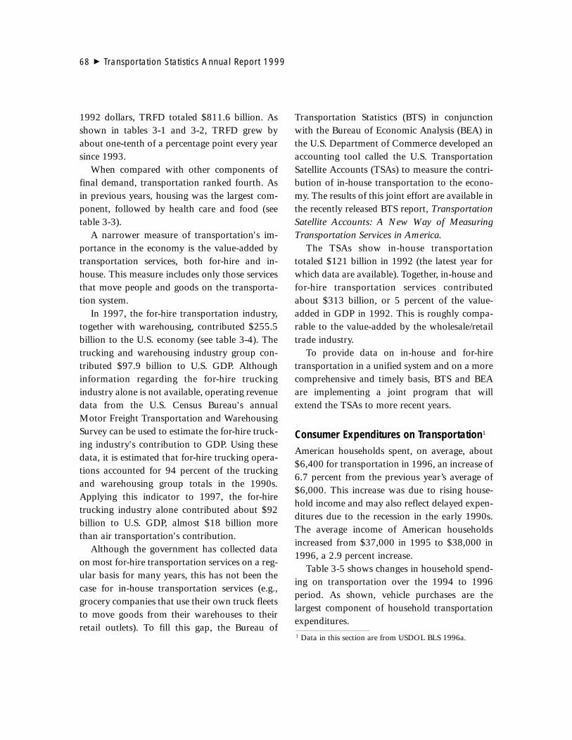
1992 dollars, TRFD totaled $811.6 billion. Asshown in tables 3-1 and 3-2, TRFD grew byabout one-tenth of a percentage point every yearsince 1993.
When compared with other components offinal demand, transportation ranked fourth. Asin previous years, housing was the largest com-ponent, followed by health care and food (seetable 3-3).
A narrower measure of transportation's im-portance in the economy is the value-added bytransportation services, both for-hire and in-house. This measure includes only those servicesthat move people and goods on the transporta-tion system.
In 1997, the for-hire transportation industry,together with warehousing, contributed $255.5billion to the U.S. economy (see table 3-4). Thetrucking and warehousing industry group con-tributed $97.9 billion to U.S. GDP. Althoughinformation regarding the for-hire truckingindustry alone is not available, operating revenuedata from the U.S. Census Bureau's annualMotor Freight Transportation and WarehousingSurvey can be used to estimate the for-hire truck-ing industry's contribution to GDP. Using thesedata, it is estimated that for-hire trucking opera-tions accounted for 94 percent of the truckingand warehousing group totals in the 1990s.Applying this indicator to 1997, the for-hiretrucking industry alone contributed about $92billion to U.S. GDP, almost $18 billion morethan air transportation's contribution.
Although the government has collected dataon most for-hire transportation services on a reg-ular basis for many years, this has not been thecase for in-house transportation services (e.g.,grocery companies that use their own truck fleetsto move goods from their warehouses to theirretail outlets). To fill this gap, the Bureau of
Transportation Statistics (BTS) in conjunctionwith the Bureau of Economic Analysis (BEA) inthe U.S. Department of Commerce developed anaccounting tool called the U.S. TransportationSatellite Accounts (TSAs) to measure the contri-bution of in-house transportation to the econo-my. The results of this joint effort are available inthe recently released BTS report, TransportationSatellite Accounts: A New Way of MeasuringTransportation Services in America.
The TSAs show in-house transportationtotaled $121 billion in 1992 (the latest year forwhich data are available). Together, in-house andfor-hire transportation services contributedabout $313 billion, or 5 percent of the value-added in GDP in 1992. This is roughly compa-rable to the value-added by the wholesale/retailtrade industry.
To provide data on in-house and for-hiretransportation in a unified system and on a morecomprehensive and timely basis, BTS and BEAare implementing a joint program that willextend the TSAs to more recent years.
Consumer Expenditures on Transportation1
American households spent, on average, about$6,400 for transportation in 1996, an increase of6.7 percent from the previous year’s average of$6,000. This increase was due to rising house-hold income and may also reflect delayed expen-ditures due to the recession in the early 1990s.The average income of American householdsincreased from $37,000 in 1995 to $38,000 in1996, a 2.9 percent increase.
Table 3-5 shows changes in household spend-ing on transportation over the 1994 to 1996period. As shown, vehicle purchases are thelargest component of household transportationexpenditures.
68 � Transportation Statistics Annual Report 1999
1 Data in this section are from USDOL BLS 1996a.

Chapter 3 Transportation and the Economy � 69
Table 3-1Transportation-Related Components of U.S. GDP: 1993–98(Current $ billions)
1993 1994 1995 1996 1997 1998
Personal consumption of transportationMotor vehicles and parts 226.2 246.6 255.4 264.8 269.5 289.4Gasoline and oil 107.6 109.4 115.6 124.5 126.5 112.6Transportation services 170.2 186.2 203.1 222.3 240.3 252.5
Total 504.0 542.2 574.1 611.6 636.3 654.5
Gross private domestic investmentTransportation structures 4.1 4.3 4.4 5.4 6.1 UTransportation equipment 99.9 118.6 126.2 137.2 152.0 U
Total 104.0 122.9 130.6 142.6 158.1 U
Exports(+)Civilian aircraft, engines, and parts 32.7 31.5 26.1 30.8 41.4 54.6Automotive vehicles, engines, and parts 52.5 57.8 61.8 65.0 74.0 72.6Passenger fares 16.6 17.1 18.9 20.4 20.9 20.8Other transportation 23.1 24.9 26.8 27.0 27.9 27.5
Total 124.9 131.3 133.6 143.2 164.2 175.5Imports(–)Civilian aircraft, engines, and parts 11.3 11.3 10.7 12.7 16.6 21.7Automotive vehicles, engines, and parts 102.4 118.3 123.8 128.9 140.8 150.3Passenger fares 11.3 12.9 14.7 15.8 18.2 18.2Other transportation 25.7 27.3 27.4 27.7 29.3 30.0
Total 150.7 169.8 176.6 185.1 204.9 220.2Net exports of transportation-related
goods and services –25.8 –38.5 –43.0 –41.9 –40.7 –44.7
Government transportation-related purchasesFederal purchases 17.6 18.8 18.1 18.9 19.7 UState and local purchases 99.8 106.5 110.0 115.5 123.1 UDefense-related purchases 9.5 8.2 8.5 8.9 8.2 8.2
Total 126.9 133.5 136.6 143.2 151.0 U
Transportation-related final demand1 709.1 760.3 798.3 855.5 905.0 UGross Domestic Product (GDP) 6,558.1 6,947.0 7,269.6 7,661.6 8,110.9 8,508.9
Total transportation in GDP (percent) 10.8 10.9 11.0 11.2 11.2 U1Demand for goods and services produced in the United States, regardless of where they are consumed. The measure counts exported goods and services,but does not include imports.
KEY: GDP = Gross Domestic Product; U = data are unavailable.
SOURCES: U.S. Department of Commerce, Bureau of Economic Analysis, Survey of Current Business, various issues, 1998, National Income and ProductAccounts tables.
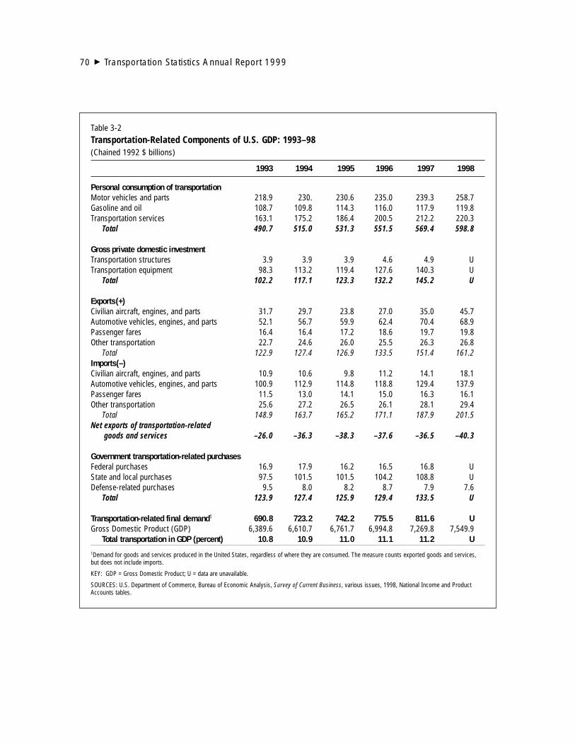
70 � Transportation Statistics Annual Report 1999
Table 3-2Transportation-Related Components of U.S. GDP: 1993–98(Chained 1992 $ billions)
1993 1994 1995 1996 1997 1998
Personal consumption of transportationMotor vehicles and parts 218.9 230. 230.6 235.0 239.3 258.7Gasoline and oil 108.7 109.8 114.3 116.0 117.9 119.8Transportation services 163.1 175.2 186.4 200.5 212.2 220.3
Total 490.7 515.0 531.3 551.5 569.4 598.8
Gross private domestic investmentTransportation structures 3.9 3.9 3.9 4.6 4.9 UTransportation equipment 98.3 113.2 119.4 127.6 140.3 U
Total 102.2 117.1 123.3 132.2 145.2 U
Exports(+)Civilian aircraft, engines, and parts 31.7 29.7 23.8 27.0 35.0 45.7Automotive vehicles, engines, and parts 52.1 56.7 59.9 62.4 70.4 68.9Passenger fares 16.4 16.4 17.2 18.6 19.7 19.8Other transportation 22.7 24.6 26.0 25.5 26.3 26.8
Total 122.9 127.4 126.9 133.5 151.4 161.2Imports(–)Civilian aircraft, engines, and parts 10.9 10.6 9.8 11.2 14.1 18.1Automotive vehicles, engines, and parts 100.9 112.9 114.8 118.8 129.4 137.9Passenger fares 11.5 13.0 14.1 15.0 16.3 16.1Other transportation 25.6 27.2 26.5 26.1 28.1 29.4
Total 148.9 163.7 165.2 171.1 187.9 201.5Net exports of transportation-related
goods and services –26.0 –36.3 –38.3 –37.6 –36.5 –40.3
Government transportation-related purchasesFederal purchases 16.9 17.9 16.2 16.5 16.8 UState and local purchases 97.5 101.5 101.5 104.2 108.8 UDefense-related purchases 9.5 8.0 8.2 8.7 7.9 7.6
Total 123.9 127.4 125.9 129.4 133.5 U
Transportation-related final demand1 690.8 723.2 742.2 775.5 811.6 UGross Domestic Product (GDP) 6,389.6 6,610.7 6,761.7 6,994.8 7,269.8 7,549.9
Total transportation in GDP (percent) 10.8 10.9 11.0 11.1 11.2 U1Demand for goods and services produced in the United States, regardless of where they are consumed. The measure counts exported goods and services,but does not include imports.
KEY: GDP = Gross Domestic Product; U = data are unavailable.
SOURCES: U.S. Department of Commerce, Bureau of Economic Analysis, Survey of Current Business, various issues, 1998, National Income and ProductAccounts tables.

� Regional DifferencesHistorically, households in the West, on average,spent more on transportation than those in theMidwest, South, and Northeast. In the pastdecade, however, household transportationexpenditures in the Midwest and Southincreased faster than in the West and Northeast.In 1995, midwestern households spent more ontransportation than any of the other threeregions. The picture changed in 1996, however,with southern households spending the most—$6,937, an increase of 15 percent over the previ-ous year. In 1996, transportation’s share in totalhousehold expenditures in the South was 21 per-cent, 3 percent higher than in the West andMidwest and 5 percent higher than in theNortheast. This increase in the South was fueledby new vehicle purchases. For example, theSouth was the only region in which households,on average, spent more than one-half of theirtransportation expenditures on purchasing vehi-cles. The share of vehicle purchases in household
Chapter 3 Transportation and the Economy � 71
Table 3-3Major Societal Functions in GDP(Current $ billions)
Societal function 1992 1997
GDP 6,244 8,111Housing 1,469 1,969Health 880 1,151Food 803 956Transportation 669 905Education 428 559Other 1,995 2,572
PercentGDP 100.0 100.0Housing 23.5 24.3Health 14.1 14.2Food 12.9 11.8Transportation 10.7 11.2Education 6.9 6.9Other 32.0 31.7
KEY: GDP = Gross Domestic Product.
NOTE: Percentages may not add due to rounding.
SOURCES: U.S. Department of Commerce, Bureau of EconomicAnalysis, Survey of Current Business, various issues, 1998,National Income and Product Accounts tables.
Table 3-4U.S. Gross Domestic Product by For-Hire Transportation Industries($ billions)
1990 1992 1997 1990 1992 1997
Gross Domestic Product 5,743.8 6,244.4 8,110.9 6,136.3 6,244.4 7,269.8
Trucking and warehousing 75.8 82.2 97.9 73.7 82.2 87.3Transportation by air 39.4 43.0 74.4 39.5 43.0 63.5Railroad transportation 19.6 22.1 24.1 18.7 22.1 28.2Incidental services 17.8 19.6 26.8 19.2 19.6 25.1Transit 9.0 10.9 13.8 10.3 10.9 11.3Water transportation 9.5 10.3 12.8 10.7 10.3 11.0Pipelines, except natural gas 5.0 4.9 5.6 4.8 4.9 6.8
Total 176.4 192.8 255.5 176.7 192.8 241.5
SOURCE: U.S.Department of Commerce, Bureau of Economic Analysis, Survey of Current Business, November 1998, GDP by Industry table.
Current dollars Chained 1992 dollars

transportation expenditures in the South was 57percent in 1996, compared with 47 percent forthe national average and 37 percent for theNortheast.
� Urban and Rural AreasSince 1992, rural households have spent more ontransportation in absolute dollar amounts thanurban households. In 1996, rural householdsspent, on average, $6,767 on transportation,$440 more than their urban counterparts.Transportation’s share of total rural householdexpenditures reached a high of 23.5 percent,while its share in urban households stayed at 18percent. This increase indicates that rural house-
hold spending on transportation grew faster thantotal expenditures. In 1995, rural households, onaverage, spent $3,300, or 55 percent of theirtransportation expenditures, on purchasing vehi-cles (including vehicle finance charges); in 1996,this expenditure reached $3,773. Transporta-tion’s share of rural household expenditures,however, remained about the same in 1996.Moreover, rural households spent more on pur-chasing used vehicles than on new ones. Usedvehicle purchases accounted for 64 percent ofrural household expenditures, compared with 54percent in urban households. Both rural andurban households sharply increased their spend-ing on purchased transportation services—17percent and 19 percent, respectively.
� Age EffectHousehold transportation expenditures, inabsolute dollar amounts, rise as the age of thehead of the household increases, peaking at the45 to 54 years of age bracket, and then declining.In 1996, households in which the head wasbetween 45 and 54 years of age spent, on aver-age, $8,233, while households in the under 25years of age bracket spent $4,029. For house-holds in which the head was 75 years of age orolder, transportation expenditures were $2,573.Transportation as a share of household expendi-tures was highest in young households. In 1996,households in the under 25 age bracket spent, onaverage, 22 percent of their total householdexpenditures on transportation. The percentagedecreased gradually as age increased, reaching itslowest point—13 percent—in households in the75 and over age bracket (see figure 3-1).
Young households also spent a higher propor-tion of their transportation expenditures on pur-chasing used vehicles than older households. Forexample, households in the youngest age groupspent 81 percent of their transportation expendi-
72 � Transportation Statistics Annual Report 1999
Table 3-5Household Transportation Expenditures:1994–96
Type of expenditure 1994 1995 1996
Average annual household transportation expenditures($ current) $6,044 $6,016 $6,382
Percentage of componentsVehicle purchasesCars and trucks, new 23.0 19.8 18.9Cars and trucks, used 21.3 23.5 24.6Other vehicles 0.7 0.6 0.6
Total 44.0 43.9 44.1
Gasoline and motor oil 16.3 16.7 16.9
Other vehicle expensesVehicle finance charges 3.9 4.3 4.3Maintenance and repairs 11.3 10.9 10.1Vehicle insurance 11.4 11.8 10.9Vehicle rental, lease, license,
and other charges 5.7 6.5 6.9Total 32.3 33.5 32.3
Purchased transportation service 6.3 5.9 6.7
SOURCES: U.S. Department of Labor, Bureau of Labor Statistics,“Consumer Expenditure Survey,” 1995, 1996, and 1997.

tures on purchasing used vehicles, while house-holds in the oldest age group spent 67 percent onnew vehicles.
The age of the head of the household alsoaffected the amount of money spent on purchasedtransportation services, such as air, ship, masstransit, and taxi fares. In 1996, households in theyoungest age bracket spent the least proportional-ly on purchased transportation services—4.6 per-cent of their transportation expenditures; theoldest age group spent the most—15 percent oftheir transportation expenditures. Moreover,households in the oldest age group spent more onintercity train services—19 percent of purchasedtransportation services, which was the highestpercentage among all age groups.
Employment in Transportation ServicesThis section examines employment in for-hiretransportation industries by sector and by occu-
pation. It also discusses wages and salaries, andlabor productivity. Employment in for-hire trans-portation industries includes all jobs, regardless ofwhat an employee actually does (e.g., driving atruck or bookkeeping). Employment in trans-portation occupations includes jobs that are spe-cific to transportation, regardless of employer(e.g., driving a truck for a trucking company orfor a retail company).
� Employment in For-Hire TransportationIndustriesTransportation industries employed about 4.2
million workers, which was 3.3 percent of thetotal U.S. civilian labor force in 1997. In the1990s, changes in the share of transportationindustry employment in the total U.S. laborforce have been within a range of 0.2 percentagepoints (USDOT Forthcoming b).
The trucking and warehousing industrygroup has been the largest transportationemployer throughout the 1980s and 1990s. Asfigure 3-2 shows, trucking and warehousingaccounted for 41 percent of total transportationindustry employment in 1997, much larger than
Chapter 3 Transportation and the Economy � 73
<25 25–34 35–44 45–54Age group
55–64 65–74 75+0
10
20
30
40
50
60
70
Share of transportationin household expenditures
Share of vehicle purchases in transportation expenditures
Share of new vehicles invehicle purchase expenditures
Share of purchased transportationservices in transportation expenditures
Share of intercity train in purchased transportation services
Percent
Figure 3-1Characteristics of Household TransportationExpenditures by Age Group
SOURCE: U.S. Department of Labor, Bureau of Labor Statistics, “ConsumerExpenditure Survey,” 1996.
Transportationservices, 11%
Air, 27%
Trucking and warehousing, 41%
Local andinterurbanpassenger
transit, 11%
Rail, water, andnon-gas pipeline, 10%
Figure 3-2Modal Share of Transportation IndustryEmployment: 1997
SOURCE: U.S. Department of Transportation, Bureau of Transportation Statistics, National Transportation Statistics 1999 (Washington, DC: Forthcoming).

the combined total of railroad, water, transit,pipeline, and transportation services. In terms ofannual growth, however, trucking and ware-housing lagged behind some modes in differentyears. For example, transit employment grew by4.7 percent in 1991, while trucking and ware-housing employment grew by 2.8 percent (seeUSDOT Forthcoming b). In 1997, the twogroups grew by 3.2 and 1.8 percent, respectively.Two trends are worth noting. First, railroadindustry employment persistently declined in the1990s, although the decline recently sloweddown from that experienced in the early part ofthe decade. Second, in recent years, employmentin the transportation services industry grewfaster than all other modes except for transit.
In 1997, the transportation industry as awhole paid $134 billion in wages and salaries,accounting for 3.4 percent of total wage andsalary accruals in the entire economy. The trans-portation industry’s share in the total declinedfrom 5.3 percent in 1960 to 4.3 percent in 1980and remained stable at 3.5 percent between 1990and 1996 (USDOT Forthcoming b).
The slight decline of transportation wages andsalaries relative to total wages and salaries can beexplained by several factors. One influencing fac-tor is the decline of transportation industryemployment as a share of the total U.S. laborforce. Another factor is the relative decrease inthe average transportation wage rate (the level ofwage or salary per full-time equivalent employ-ee). In 1980, the annual wage rate in the trans-portation industry was 32 percent higher than theaverage wage for the entire U.S. labor force. Thatadvantage declined to 20 percent in 1985 and to10 percent in 1990. By 1997, the transportationwage rate was only about 3 percent higher thanthe national average (USDOT Forthcoming b).
Not surprisingly, the distribution of the trans-portation industry’s total wages and salariesamong modes follows a pattern similar to that in
the employment data, with the trucking andwarehousing industry group’s share accountingfor a little over 38 percent of the total in 1997.The railroad industry’s share decreased dramati-cally, from almost 38 percent in 1960 to less than9 percent in 1997. In contrast, the air trans-portation industry’s share went from under 9percent in 1960 to over 30 percent in 1997(USDOT Forthcoming b).
Wage rates for a particular industry indicatehow well paid employees are in that industry.The average wage rate for the transportationindustry as a whole has declined relative to theaverage wage rate for the entire U.S. labor force.
The local and interurban passenger transitindustry falls below all other modes in wagerates. The next lowest was the trucking and ware-housing industry. At $31,700 in 1997, truckingand warehousing industry wages were more than8 percent lower than the average for the trans-portation industry as a whole and 5 percentlower than the national average. The pipelineindustry, which has the lowest wage and salarytotal, pays the highest wage rate. In 1997, thepipeline industry’s wage rate, at $60,000, wasalmost triple the transit wage rate and nearlydouble the trucking and warehousing industrywage rate (USDOT Forthcoming b).
� Employment in Transportation OccupationsEmployment in transportation occupations coversevery industry but includes only people with skillsspecific to transportation, such as truck driversand airline pilots. As the only employment mea-sure that includes transportation-specific employ-ment within nontransportation industries,transportation occupation data are useful in esti-mating transportation operations outside as wellas within for-hire transportation industries(USDOT Forthcoming b).
In 1997, employment in transportation occu-pations was 4.5 million workers, or 3.5 percent
74 � Transportation Statistics Annual Report 1999

of all employed workers 16 years of age andover. Although employment in transportationoccupations increased by 85,000 workers in1997, transportation’s share in the total employ-ment decreased slightly because total employ-ment increased faster than transportationemployment. From 1990 to 1997, however, dif-ferences between the growth rates of transporta-tion industry employment and transportationoccupational employment have been small.
As mentioned earlier, information on the dis-tribution of transportation occupational employ-ment provides an indicator of the magnitude oftransportation operations inside and outsidetransportation industries. The National In-dustry-Occupation Employment Matrix fromthe Bureau of Labor Statistics provides data onthe industrial distribution of occupationalemployment. The latest matrix is for 1996 andshows that within the transportation industrygroup 1.5 million workers (36 percent of thetotal) were employed in transportation occupa-tions (USDOL BLS 1996b). Most were truck dri-vers, 62 percent, and bus drivers, 12 percent.
Nontransportation industries employed near-ly two-thirds of the workers in transportationoccupations in 1996. The wholesale and retailtrade industry employed almost half of theseworkers, with truck driving as the predominantoccupation. The service industry is the thirdlargest employer of transportation occupationalworkers—mostly bus drivers. The governmentemployed more people in transportation occupa-tions than the agriculture, mining, communica-tions and utilities, and finance, insurance, andreal estate industries combined.
Figure 3-3 shows the distribution of totaltransportation occupational employment in1997. Truck drivers, including drivers of heavyand light trucks, accounted for the largest per-centage (67.8 percent) of those employed intransportation occupations. This percentage,
which was the same as in the previous year, was2.7 percent higher than in 1990 (USDOTForthcoming b). Throughout the 1980s andearly 1990s, truck drivers accounted for about65 percent of all employed transportation occu-pational workers, although the higher shares inmore recent years may point to a new pattern.Employment in air transportation occupationsgrew the fastest in 1997, posting a 12.4 percentgain. In contrast, in 1997, employment in truck-ing occupations grew 1.9 percent, while bus dri-vers and water transportation occupationsdeclined by 8 and 26 percent, respectively.
Information on occupational wages andsalaries for transportation is not as extensive asthat on industry wages and salaries. Based onavailable data, airplane pilots and navigators arepaid the highest wage, while bus drivers and taxidrivers are paid the lowest.
Although earnings differentials among majortransportation occupations have remained stablesince the mid-1980s, earnings for different trans-portation occupations often fluctuated (USDOTForthcoming b).
Chapter 3 Transportation and the Economy � 75
Truck drivers, 68%
Bus drivers, 10%
Other motor vehicle operators, 12%
Rail transportation, 3%Water transportation, 1%Air transportation, 3%
Public transportationattendants, 3%
Figure 3-3Employment in TransportationOccupations: 1997
SOURCE: U.S. Department of Transportation, Bureau of Transportation Statistics, National Transportation Statistics 1999 (Washington, DC: Forthcoming).
Labor Productivity in TransportationTransportation labor productivity measures theratio of transportation output and transporta-tion labor input. Transportation output is usu-ally measured by quality-adjusted ton-milesand passenger-miles, and transportation inputis usually measured by the number of trans-portation employees or employee-hours.Because of data limitations, this section discuss-es productivity measures based on the numberof employees only. Regardless of how outputand input are measured, labor productivitymeasures only show how productive labor is,not why labor is productive. Also, becauselabor productivity measures are most oftenconducted on an industry-by-industry basis,they do not provide information about the pro-ductivity of workers in transportation occupa-tions (USDOL BLS OPT 1999).
From 1990 to 1996, the output of the railroadindustry (measured by an index of passenger-miles, freight ton-miles, revenue, and other fac-tors) went up by 21.2 percent, while its inputwent down by 16.1 percent. As a result, railroadlabor productivity went up by 44.5 percent.Productivity increased even more in the 1980s,posting a 106 percent increase. On average, rail-road labor productivity improved by 4.5 percentannually from 1947 to 1996 (USDOL BLS OPT1999).
In contrast, labor productivity in the truckingindustry increased much more slowly. From1990 to 1996, output per employee went up by17.7 percent. As in the railroad industry, laborproductivity in the trucking industry increasedmuch faster from 1981 to 1990—32.9 percent—but still much slower than the railroad industryduring the same period. From 1954 to 1996,labor productivity in the trucking industry roseby 2.8 percent each year, considerably less thanthat recorded by the railroad industry (USDOLBLS OPT 1999).
The air transportation industry (both passen-ger and freight) enjoyed the fastest labor produc-tivity growth over the 1947 to 1996 period—5.6percent annually. Its growth rate between 1990and 1996 was 19.5 percent, faster than thetrucking industry but much slower than the rail-road industry (USDOL BLS OPT 1999).
From 1947 to 1996, the average annualgrowth in labor productivity in the petroleumpipelines industry was similar to that in the airtransportation industry. In the 1990s, however,productivity growth in the petroleum pipelinesindustry exceeded that in the air transportationindustry (36.1 percent vs. 19.5 percent) (USDOLBLS OPT 1999).
Of all the modes, Class I bus carriers had thelowest productivity, with considerable industryfluctuation in the 1980s and 1990s. From 1954to 1996, labor productivity decreased 0.3 per-cent each year on average, the combined result ofdecreasing labor input and a more rapidlydecreasing output (USDOL BLS OPT 1999).
Figure 3-4 displays trends in labor productiv-ity between 1955 and 1996 for the five trans-portation industries discussed above. Manyfactors contribute to the level of labor produc-tivity and its changes over time. One factor is theavailability of transportation capital and thelevel of technologies embodied in the capital.Transportation capital includes both transporta-tion equipment, such as locomotives, and trans-portation-related structures, such as airports.Other factors include transportation-relatedhuman capital, infrastructure, and governmentregulations. It is not clear how these factorsinteract to influence labor productivity growthor how important each factor is. In some cases,changes in labor productivity may have been dri-ven by factors that have nothing to do withlabor. For example, improvements in a road orbusiness logistics may make truck driving moreproductive.
76 � Transportation Statistics Annual Report 1999

Chapter 3 Transportation and the Economy � 77
Figure 3-4Labor Productivity Trends by Mode
NOTES: Output is measured by quality-adjusted ton-miles and passenger-miles for railroad and air transportation, quality-adjusted ton-miles for trucking andpipelines, and passenger-miles for buses. No data are available for water transportation.
SOURCE: U.S. Department of Labor, Bureau of Labor Statistics, Office of Productivity and Technology, 1999.
01955 1960 1965 1970 1975 1980 1985 1990 1995
200100
300400500600700800900
Index: 1955 = 100
Railroad Bus
Trucking Air
01955 1960 1965 1970 1975 1980 1985 1990 1995
200100
300400500600700800900
01955 1960 1965 1970 1975 1980 1985 1990 1995
200100
300400500600700800900
Pipelines
01955 1960 1965 1970 1975 1980 1985 1990 1995
200100
300400500600700800900
01955 1960 1965 1970 1975 1980 1985 1990 1995
200100
300400500600700800900

PUBLIC TRANSPORTATIONREVENUES AND EXPENDITURES
All levels of government play important roles intransportation by contributing to transporta-tion-related final demand and labor productivitygrowth. This section provides summary informa-tion on government revenues and expenditureson transportation, including capital investment.2
Government Revenues from TransportationIn fiscal year (FY) 1995, government revenuesfrom all transportation modes reached $93.7billion (current dollars). Adjusted for price increas-es, government transportation revenues increasedfrom $83.5 billion in 1994 to $86.7 billion in 1995(USDOT Forthcoming a, tables A-1, A-2). Figure3-5 shows that the annual growth rate in govern-ment transportation revenues fluctuated consider-ably between 1986 and 1995. The parallel trend inconstant and current dollar growth rates indicatesthat the inflationary impact on government trans-portation revenues stayed fairly constant over thisperiod, although it seems to have declined slightlyin the first half of the 1990s.
Almost half of the government transportationrevenues are raised by states. In 1995, state gov-ernment revenues accounted for 48 percent of thetotal, while federal and local revenues were 32and 20 percent, respectively (USDOT Forth-coming a). Since the mid-1980s, the share of totaltransportation revenues among the three levels ofgovernment has remained stable. For example, in
1985 the federal government’s share was 34 per-cent, while state and local governments’ shareswere 48 percent and 18 percent, respectively.
Highways generated $66.74 billion (71 per-cent) in government transportation revenues in1995 (see figure 3-6). Pipeline transportation rev-enues were the lowest of all modes, accountingfor just $35 million out of $93.7 billion in 1996.The proportions of revenues collected by variouslevels of government from different modes fluctu-ates from year to year. In 1996, for example, stategovernments received a large share of revenuesfrom highway transportation, while local govern-ments received the most from air transportationand transit, and the federal government receivedthe largest share from pipelines and water trans-portation. At other times, the pattern has dif-fered. For example, local governments collectedhalf the water revenues from 1985 to 1989, anduntil 1993 the federal government’s share of rev-enues from air transportation was larger thanthose of state and local governments.
Fuel taxes are important sources of revenue forfederal and state governments. The bulk of fueltaxes comes from the highway mode. At the fed-eral level, gasoline and diesel fuel taxes providedmore than 85.8 percent of total highway trustfund revenues in fiscal year (FY) 1995. At thestate level, motor fuel taxes accounted for almost60 percent of total state highway revenues.Motor fuel tax receipts are a far less importantportion of revenues for local governments thanfor federal and state governments. Property taxrevenues are a far greater income source for localgovernments than motor fuel taxes. Fuel taxesare less important as a source of government rev-enues from other modes of transportation. Fueltaxes accounted for only 3.4 percent of totalFederal Airport and Airway Trust Fund revenuesin FY 1995. In the same year, the inland water-way fuel tax accounted for 6.1 percent of thetotal federal receipts from water transportation
78 � Transportation Statistics Annual Report 1999
2Statistics in this section are based on data from the U.S.Department of Commerce, Census Bureau, which uses dif-ferent definitions and accounting methods from those usedby some modal administrations of the U.S. Department ofTransportation. For example, revenues in this section arelimited to gasoline taxes, tolls, and other sources that arecollected directly from transportation users. Revenue statis-tics published by the Federal Highway Administration alsoinclude items such as investment income and other taxesand fees.

(USDOT Forthcoming a). Similar information isnot available for state and local government rev-enues from these and other modes.
Government Expenditures on TransportationIn FY 1995, all levels of government spent$129.3 billion (current dollars) on all modes oftransportation. (Federal grants are included butnot double counted.) Figure 3-7 shows thatgrowth in government transportation expendi-tures in current and constant dollars followed asimilar trend, but it is important to note that pricechanges had a greater impact on current dollarexpenditures in the late 1980s and early 1990s.
Excluding federal grants, state and local gov-ernments spent $89.36 billion (current dollars) orabout 69.1 percent of total government trans-portation expenditures in 1995. This is about thesame as their shares in total transportation rev-enues. Since the mid-1980s, the distribution oftotal transportation expenditures among thethree levels of governments is almost identical tothe distribution of total transportation revenues.From 1985 to 1995, the federal and the state andlocal governments’ shares in total governmenttransportation revenues and expenditures aver-aged 32 and 68 percent, respectively.
Chapter 3 Transportation and the Economy � 79
1986 1987 1988 1989 1990 1991 1992 1993 1994 1995–2
0
2
4
6
8
10
12
$ Constant
$ Current
Percent
Figure 3-5Growth in Government Transportation Revenues: 1986–95
SOURCE: U.S. Department of Transportation, Bureau of TransportationStatistics, Government Transportation Financial Statistics: Fiscal Years1985–95, forthcoming on the BTS website at www.bts.gov.
Air, 15%
Transit, 10% Water, 4%
Pipeline, 0%
Highway, 71%
Figure 3-6Government Transportation Revenues by Mode:Fiscal Year 1995
SOURCE: U.S. Department of Transportation, Bureau of TransportationStatistics, Government Transportation Financial Statistics: Fiscal Years1985–95, forthcoming on the BTS website at www.bts.gov.
1986 1987 1988 1989 1990 1991 1992 1993 1994 1995
Figure 3-7Growth in Government Transportation Expenditures: 1986–95
SOURCE: U.S. Department of Transportation, Bureau of TransportationStatistics, Government Transportation Financial Statistics: Fiscal Years1985–95, forthcoming on the BTS website at www.bts.gov.
0
1
2
3
4
5
6
7
8
9
10Percent
Current $
Constant $
As discussed here, the near equality of theshares of revenues and expenditures is due toexpenditures reflecting each level of governmentusing their own funds before federal grants aretransferred. Since most federal governmentexpenditures on transportation are in the form ofgrants to states and localities, expenditures afterfederal grants present a very different picture. InFY 1995, 63 percent of the $39.93 billion in fed-eral government expenditures on transportationwere grants to state and local governments. Thebalance was spent directly by the federal govern-ment. Including federal grants, state and localgovernments accounted for about 86 percent ofthe $129.3 billion of total government trans-portation expenditures. Between state and localgovernments, local governments spend morethan state governments overall. In 1995, thelocal government share of the state and localtotal direct expenditures was 54 percent(USDOT Forthcoming a).
Governments spent more on highways than onall other modes combined. In 1995, total highwayspending was $79.2 billion, about 61 percent oftotal government transportation expenditures.Nearly three-quarters of this amount was spent bystate and local governments. Transit expendituresaccounted for nearly 20 percent of the total;pipelines received only $42 million, less than one-third of one-tenth of a percent (USDOT BTSForthcoming a). A comparison among modesindicates that the federal government spends moreon air, water, and rail; state and local govern-ments, using their own funds, spend more onhighways, transit, and pipelines. In 1995, federalgovernment spending (directly and throughgrants) on air and water amounted to about 61percent of total government expenditures on thesemodes and almost all of government expenditureson rail (USDOT Forthcoming a). In contrast, stateand local government expenditures on transit andpipelines amounted to 82.6 percent and 57.1 per-
cent, respectively, of total government spendingon these modes.
CAPITAL INVESTMENT AND CAPITAL STOCK
An important category of government trans-portation expenditures is capital investment,which includes infrastructure and equipment.Transportation infrastructure is a comprehensiveterm used to describe a variety of fixed structuresand facilities used by all modes of transportation.
Generally, transportation infrastructure in itsphysical form includes railroads, highways andstreets, bridges and tunnels, airports and air-ways, ports and waterways, mass transit facili-ties, and pipelines. Except for railroads andpipelines, transportation infrastructure in theUnited States relies largely on public investmentsand some joint investments between the publicand private sectors.
In 1995, all levels of government invested$60.6 billion, accounting for 46.9 percent oftotal government transportation expenditures.Not surprisingly, highways received the lion’sshare, with 71 percent of the total, while airtransportation and transit received 12.9 and12.4 percent of the total, respectively (USDOTForthcoming a).
In terms of the investment proportion of totalgovernment expenditures, the ranking amongdifferent modes is slightly different. For example,for each dollar spent on railroad transportation,more than 55 cents was invested in capital stock;for each dollar spent on highways, 54 cents wentto capital investments. For all other modes,except air, the government invested 26 cents ofevery dollar spent on these modes in capitalstock. Air transportation had the lowest govern-ment investment ratio of 23.7 percent (USDOTForthcoming a).
80 � Transportation Statistics Annual Report 1999

Over a period of decades, government invest-ments in transportation infrastructure haveresulted in a huge transportation infrastructurecapital stock that constitutes a significant andintegral component of the total national wealthand productive capacity. Based on estimatesfrom the national economic accounts, publiccapital stock in highways and streets was worth$1.3 trillion in 1996. State and local govern-ments own nearly all (98.1 percent) of this capi-tal stock (see table 3-6).
Governments invest in other types of trans-portation infrastructures as well, but detaileddata are not available on these investments. Tobetter manage transportation infrastructure, cal-culate its contribution to the U.S. economy, andplan its future expansion, estimates are neededon the size and scope of the total capital stockand also for specific types of assets. These andother data needs are discussed in chapter 6.
DATA NEEDS
Since the mid-1980s, many attempts have beenmade to understand how public investments intransportation infrastructure contribute to pri-vate production and changes in productivity andeconomic growth. Inadequate capital stock dataoften hinder these analyses.
Although total transportation infrastructurecost can be calculated from past investments, cap-
ital stock data are required to determine howmuch of the cost is embodied in commodities andservices provided by various sectors of the econo-my because of their use of the infrastructure.
Another important use of transportation infra-structure capital stock data is to assist in deter-mining investment needs. From the perspective ofmaintaining capital stock value and long-termnational wealth, information on the level andcondition of capital stock can be used to estimatehow much capital stock has depreciated. To keepcapital stock intact, investments are needed tocompensate for depreciation. From the perspec-tive of maintaining or expanding capital stock tomeet the need for capital services, information onthe existing stock’s capacity to provide such ser-vices is required to estimate investment needs.
The current official statistics, however, do notcompletely satisfy these information require-ments because they either do not provide thenecessary details or are developed within frame-works that are appropriate to some, but not all,data needs. Since market transactions do notexist for most uses of public transportation infra-structure, data on infrastructure cost at the userlevel cannot be directly collected. To fill this datagap, the Bureau of Transportation Statistics iscurrently implementing a statistical program toestimate transportation infrastructure capitalstock of all transportation modes at national andindividual state levels.
Chapter 3 Transportation and the Economy � 81
Table 3-6Net Capital Stock of Highways and Streets(Current $ billions)
1986 1988 1990 1992 1994 1996
Federal 18.7 19.8 20.7 20.7 22.2 23.8State and local 798.6 866.7 950.4 997.6 1,111.4 1262.5
Total 817.3 886.5 971.1 1,018.3 1,133.6 1,286.3
SOURCE: U.S. Department of Commerce, Bureau of Economic Analysis, Survey of Current Business, September 1997.

REFERENCES
U.S. Department of Commerce (USDOC), Bureauof Economic Analysis (BEA). 1997. Survey ofCurrent Business. September.
____. 1998. Survey of Current Business.
U.S. Department of Labor (USDOL), Bureau ofLabor Statistics (BLS). 1996a. ConsumerExpenditure Survey.
____. 1996b. National Industry Occupation:Employment Matrix. Available at www.stats.bls.gov/asp/oep/nioem/empiohm.asp.
U.S. Department of Labor (USDOL), Bureau ofLabor Statistics (BLS), Office of Productivityand Technology (OPT). 1999. Personal com-munication.
U.S. Department of Transportation (USDOT),Bureau of Transportation Statistics. Forth-coming a. Government Transportation Finan-cial Statistics: Fiscal Years 1985–95. Availableon the BTS website: www.bts.gov.
____. Forthcoming b. National TransportationStatistics 1999. Washington, DC.
82 � Transportation Statistics Annual Report 1999
The highest priority of the U.S. Department of Transportation (DOT) is to“promote public health and safety by working toward the elimination oftransportation-related deaths, injuries, and property damage” (USDOT
NHTSA 1997). Although great progress has been made in the last few decades,transportation crashes remain the leading cause of accidental deaths and injuries inthe United States, claiming tens of thousands of lives, and injuring millions of peo-ple each year. Most of the transportation deaths (about 95 percent) and injuries (aneven higher percentage) occur on the nation’s highways.
Although many safety issues are specific to a particular mode, others cut acrossmodes. This chapter briefly discusses mode-by-mode trends, but concentrates oncross-modal issues.1 Following a review of long-term transportation safety trends,the chapter discusses four special concerns—safe transportation to and from schools,pedestrian and bicycle safety, security of transportation systems against crime andterrorism, and international trends in road safety—as well as data needs.
Safely transporting students to and from schools is of particular interest to thepublic. Congress, in the Transportation Equity Act for the 21st Century (Public Law105-178), known as TEA-21, mandated DOT to undertake a special study of safety
�
83
Transportation Safety
chapter four
1 For a more detailed discussion of mode-by-mode trends, see chapter 3 in the past three issues of theTransportation Statistics Annual Report (TSAR). Cross-modal topics discussed in these issues include: inTSAR98—transportation and the elderly, causes of crashes, and alcohol and drug involvement; inTSAR97—child safety, safety of transportation workers, and hazardous materials; in TSAR 96—fatigue,highway-rail grade crossings, safety technologies, and alcohol and drug involvement.

issues in transporting school children using vari-ous modes, which is due in 2001.
Walking and biking are often promoted ashealthy, nonpolluting forms of transportationthat could help alleviate congestion. However,walkers and bicyclists account for roughly 15percent of fatalities involving motor vehicles, andtheir safety is an important concern.
In a pervasively integrated world economy,with more Americans traveling abroad for busi-ness and pleasure, international trends in trans-portation safety and security are of interest.Transportation, particularly air travel and masstransit can be targets of terrorists: for example,the gas attack on the Tokyo subway. Air travel-ers now regard precautions against terrorism asa routine part of air travel. In addition, this chap-ter briefly highlights road safety issues in othercountries, as U.S. citizens traveling abroad whouse taxis, buses, or rental cars may encountertraffic safety conditions that can differ fromthose in the United States.
LONG-TERM TRENDS
Table 4-1 shows historical trends in absolute num-bers of fatalities, injuries, and crashes/accidents forall modes. The data show that in the last threedecades, transportation fatalities have decreasedfor most modes. The figures for rail and transitinclude fatalities and injuries arising from certaintypes of incidents involving no moving vehicle(e.g., falls on transit property or fires in railroadrepair sheds). Thus, the data in table 4-1 for tran-sit and rail include many nonpassengers, makingcomparisons with other modes difficult.
Table 4-2 shows the distribution of fatalitiesin 1997. Occupants of cars and light trucksaccounted for nearly three-quarters of the fatali-ties, and motorcyclists slightly under 5 percent,while pedestrians and pedalcyclists hit by motorvehicles accounted for just under 14 percent of
the fatalities. Recreational boating and generalaviation accounted for over 3 percent of thefatalities—more than all of the listed commercialpassenger modes and freight trains combined.
Table 4-3 provides historical detail for thehighway mode, which accounts for most trans-portation fatalities and injuries. As shown, thereare fewer fatalities involving motor vehicles todaythan in the mid-1970s or early-1980s, eventhough miles of travel have increased. The declineis evident across most highway submodes, withthe conspicuous exception of light trucks (e.g.,sport utility vehicles, vans, and pickup trucks).The number of such vehicles increased dramati-cally over the period; they now account for aboutone-third of the motor vehicle fleet. The implica-tions of these vehicles for highway safety is receiv-ing considerable scrutiny. For example, sportutility vehicles have the highest rollover involve-ment rate by far of any vehicles in fatal crashes—36 percent compared with 15 percent forpassenger cars (USDOT NHTSA 1998b).
Considerable concern also exists about theincreasing number of crashes involving light trucksand passenger cars. A study sponsored by theNational Highway Traffic Safety Administration(NHTSA) concluded that approximately twice asmany car drivers would die in collisions with lighttrucks than in similar collisions involving cars of thesame weight as the light truck (Joksch 1998, xi).
For systematic analyses of transportation safe-ty trends, it is customary to calculate safety ratesby dividing the absolute numbers of fatalities (orother adverse outcome) by some measure ofactivity, such as number of trips, miles traveled,or hours of vehicle operation. The logic for doingthis is straightforward; people are exposed totransportation risks primarily when they travel.Hence, everything else remaining the same, themore travel there is, the more risk people incur.Thus, it can be misleading to use absolute num-bers of, say, fatalities to compare the safety of a
84 � Transportation Statistics Annual Report 1999
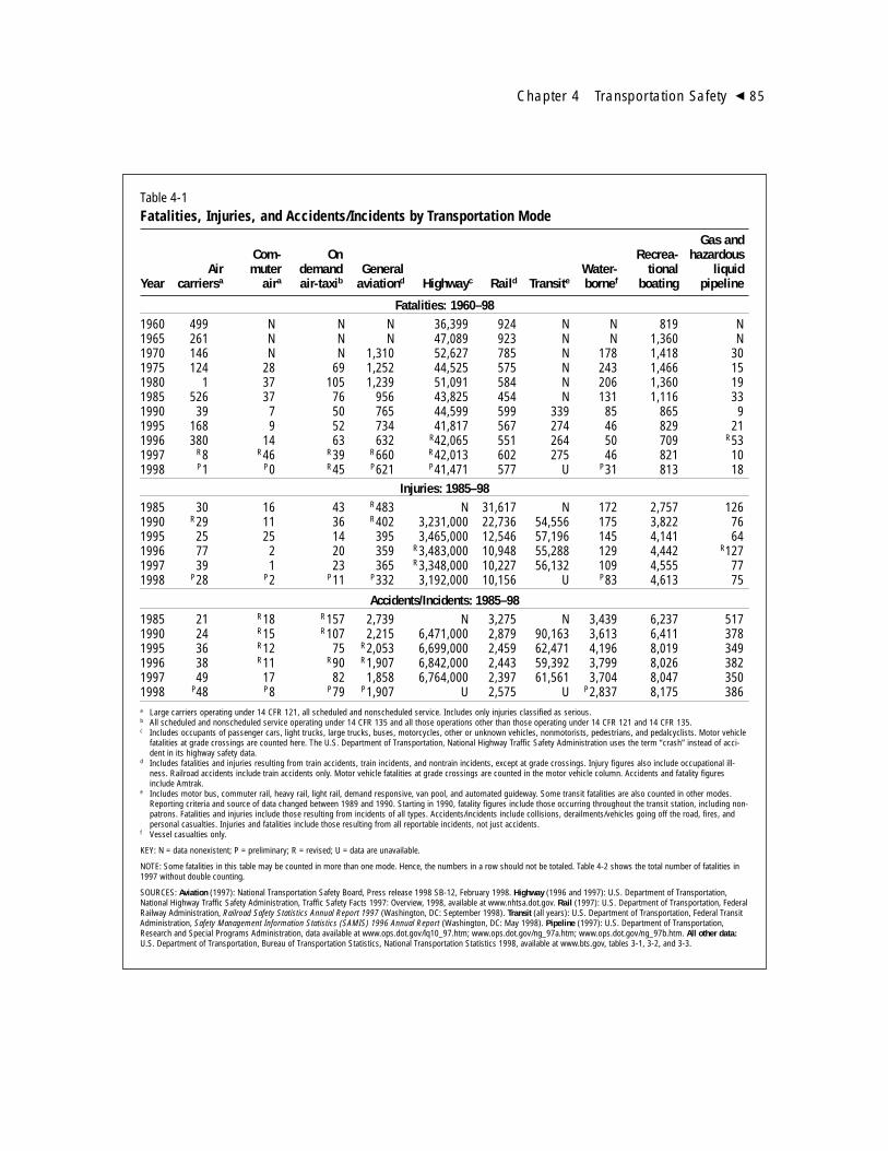
Chapter 4 Transportation Safety � 85
Table 4-1Fatalities, Injuries, and Accidents/Incidents by Transportation Mode
Gas andCom- On Recrea- hazardous
Air muter demand General Water- tional liquidYear carriersa aira air-taxib aviationd Highwayc Raild Transite bornef boating pipeline
Fatalities: 1960–981960 499 N N N 36,399 924 N N 819 N1965 261 N N N 47,089 923 N N 1,360 N1970 146 N N 1,310 52,627 785 N 178 1,418 301975 124 28 69 1,252 44,525 575 N 243 1,466 151980 1 37 105 1,239 51,091 584 N 206 1,360 191985 526 37 76 956 43,825 454 N 131 1,116 331990 39 7 50 765 44,599 599 339 85 865 91995 168 9 52 734 41,817 567 274 46 829 211996 380 14 63 632 R42,065 551 264 50 709 R531997 R8 R46 R39 R660 R42,013 602 275 46 821 101998 P1 P0 R45 P621 P41,471 577 U P31 813 18
Injuries: 1985–981985 30 16 43 R483 N 31,617 N 172 2,757 1261990 R29 11 36 R402 3,231,000 22,736 54,556 175 3,822 761995 25 25 14 395 3,465,000 12,546 57,196 145 4,141 641996 77 2 20 359 R3,483,000 10,948 55,288 129 4,442 R1271997 39 1 23 365 R3,348,000 10,227 56,132 109 4,555 771998 P28 P2 P11 P332 3,192,000 10,156 U P83 4,613 75
Accidents/Incidents: 1985–981985 21 R18 R157 2,739 N 3,275 N 3,439 6,237 5171990 24 R15 R107 2,215 6,471,000 2,879 90,163 3,613 6,411 3781995 36 R12 75 R2,053 6,699,000 2,459 62,471 4,196 8,019 3491996 38 R11 R90 R1,907 6,842,000 2,443 59,392 3,799 8,026 3821997 49 17 82 1,858 6,764,000 2,397 61,561 3,704 8,047 3501998 P48 P8 P79 P1,907 U 2,575 U P2,837 8,175 386a Large carriers operating under 14 CFR 121, all scheduled and nonscheduled service. Includes only injuries classified as serious.b All scheduled and nonscheduled service operating under 14 CFR 135 and all those operations other than those operating under 14 CFR 121 and 14 CFR 135.c Includes occupants of passenger cars, light trucks, large trucks, buses, motorcycles, other or unknown vehicles, nonmotorists, pedestrians, and pedalcyclists. Motor vehicle
fatalities at grade crossings are counted here. The U.S. Department of Transportation, National Highway Traffic Safety Administration uses the term “crash” instead of acci-dent in its highway safety data.
d Includes fatalities and injuries resulting from train accidents, train incidents, and nontrain incidents, except at grade crossings. Injury figures also include occupational ill-ness. Railroad accidents include train accidents only. Motor vehicle fatalities at grade crossings are counted in the motor vehicle column. Accidents and fatality figuresinclude Amtrak.
e Includes motor bus, commuter rail, heavy rail, light rail, demand responsive, van pool, and automated guideway. Some transit fatalities are also counted in other modes.Reporting criteria and source of data changed between 1989 and 1990. Starting in 1990, fatality figures include those occurring throughout the transit station, including non-patrons. Fatalities and injuries include those resulting from incidents of all types. Accidents/incidents include collisions, derailments/vehicles going off the road, fires, andpersonal casualties. Injuries and fatalities include those resulting from all reportable incidents, not just accidents.
f Vessel casualties only.
KEY: N = data nonexistent; P = preliminary; R = revised; U = data are unavailable.
NOTE: Some fatalities in this table may be counted in more than one mode. Hence, the numbers in a row should not be totaled. Table 4-2 shows the total number of fatalities in1997 without double counting.
SOURCES: Aviation (1997): National Transportation Safety Board, Press release 1998 SB-12, February 1998. Highway (1996 and 1997): U.S. Department of Transportation,National Highway Traffic Safety Administration, Traffic Safety Facts 1997: Overview, 1998, available at www.nhtsa.dot.gov. Rail (1997): U.S. Department of Transportation, FederalRailway Administration, Railroad Safety Statistics Annual Report 1997 (Washington, DC: September 1998). Transit (all years): U.S. Department of Transportation, Federal TransitAdministration, Safety Management Information Statistics (SAMIS) 1996 Annual Report (Washington, DC: May 1998). Pipeline (1997): U.S. Department of Transportation,Research and Special Programs Administration, data available at www.ops.dot.gov/lq10_97.htm; www.ops.dot.gov/ng_97a.htm; www.ops.dot.gov/ng_97b.htm. All other data:U.S. Department of Transportation, Bureau of Transportation Statistics, National Transportation Statistics 1998, available at www.bts.gov, tables 3-1, 3-2, and 3-3.

86 � Transportation Statistics Annual Report 1999
Table 4-2Detailed Distribution of Transportation Fatalities by Mode: 1997
Categorya 1997 Percent
Passenger car occupants 22,199 50.0Light-truck occupants 10,249 23.1Pedestrians struck by motor vehicles 5,321 12.0Motorcyclists 2,116 4.8Recreational boating 821 1.8Pedalcyclists struck by motor vehicles 814 1.8Large-truck occupants 723 1.6General aviation 660 1.5Railroadb 602 1.4Other and unknown motor vehicle occupants 420 0.9Other nonoccupants in highway crashesc 153 0.3Heavy-rail transit (subway) 77 0.2Waterborne transportation (vessel casualties only) 46 0.1Commuter air 46 0.1Grade crossings, not involving motor vehiclesd 42 0.1Air taxi 39 0.1Bus occupants (school, intercity, and transit) 18 0.04Gas distribution pipelines 9 0.02Transit buses, fatalities not related to accidentse 9 0.02Part 121 air carriers 8 0.02Demand responsive/vanpool transit, fatalities not related to accidentsf 5 0.01Light rail 3 <0.01Gas transmission pipelines 1 <0.01
Total 44,381
Other counts, redundant with aboveg
Grade crossings, with motor vehicles 419Transit buses, accident-related fatalities 100Commuter rail 79Passengers on railroad trains 6Demand responsive service, accident-related fatalities 2a Unless specified as occupants, includes fatalities outside the vehicle.b Includes fatalities outside trains, except at grade crossings.c Includes all nonoccupant fatalities, except pedalcyclists and pedestrians.d Grade-crossing fatalities involving motor vehicles are included in counts for motor vehicles.e Includes school, intercity, and transit bus occupants.f Fatalities not related to accidents for transit buses and demand responsive transit are not included under highway submodes. Accidents include collisions
and derailments/buses leaving the road.g Fatalities at grade crossings with motor vehicles are included under relevant motor vehicle modes. Commuter rail fatalities are counted under railroad. For
transit bus and demand responsive transit accidents, occupant fatalities are counted under “bus” and nonoccupant fatalities are counted under “pedestri-ans,” “pedalcyclists,” or other motor vehicle categories.
SOURCES: Aviation (1997): National Transportation Safety Board, Press release 1998 SB-12, February 1998. Highway (1996 and 1997): U.S. Department ofTransportation, National Highway Traffic Safety Administration, Traffic Safety Facts 1998: Overview, 1999, available at www.nhtsa.dot.gov. Rail (1997): U.S.Department of Transportation, Federal Railway Administration. Railroad Safety Statistics Annual Report 1997 (Washington, DC: September 1998). Transit (allyears): U.S. Department of Transportation, Federal Transit Administration, Safety Management Information Statistics (SAMIS) 1997 Annual Report(Washington, DC: March 1999). Pipeline (1997): U.S. Department of Transportation, Research and Special Programs Administration, data available atwww.ops.dot.gov/lq10_97.htm; www.ops.dot.gov/ng_97a.htm; www.ops.dot.gov/ng_97b.htm. All other data: U.S. Department of Transportation, Bureau ofTransportation Statistics, National Transportation Statistics 1998, available at www.bts.gov, tables 3-1, 3-2, and 3-3.

Chapter 4 Transportation Safety � 87
Table 4-3Highway Fatalities and Injuries by Occupant and Nonoccupant Category
Other/ Other/ All occupantPas- unknown unknown and non-
senger Light Large Motor- vehicle Pedes- Pedal- non- occupantYear car truck truck Bus cycle occupants trians cyclists occupants categories
Fatalities: 1975–98
1975 25,929 4,856 961 53 3,189 937 7,516 1,003 81 44,5251976 26,166 5,438 1,132 73 3,312 981 7,427 914 80 45,5231977 26,782 5,976 1,287 42 4,104 959 7,732 922 74 47,8781978 28,153 6,745 1,395 41 4,577 622 7,795 892 111 50,3311979 27,808 7,178 1,432 39 4,894 579 8,096 932 135 51,0931980 27,449 7,486 1,262 46 5,144 540 8,070 965 129 51,0911981 26,645 7,081 1,133 56 4,906 603 7,837 936 104 49,3011982 23,330 6,359 944 35 4,453 525 7,331 883 85 43,9451983 22,979 6,202 982 53 4,265 362 6,826 839 81 42,5891984 23,620 6,496 1,074 46 4,608 440 7,025 849 99 44,2571985 23,212 6,689 977 57 4,564 544 6,808 890 84 43,8251986 24,944 7,317 926 39 4,566 442 6,779 941 133 46,0871987 25,132 8,058 852 51 4,036 436 6,745 948 132 46,3901988 25,808 8,306 911 54 3,662 429 6,870 911 136 47,0871989 25,063 8,551 858 50 3,141 424 6,556 832 107 45,5821990 24,092 8,601 705 32 3,244 460 6,482 859 124 44,5991991 22,385 8,391 661 31 2,806 466 5,801 843 124 41,5081992 21,387 8,098 585 28 2,395 387 5,549 723 98 39,2501993 21,566 8,511 605 18 2,449 425 5,649 816 111 40,1501994 21,997 8,904 670 18 2,320 409 5,489 802 107 40,7161995 22,423 9,568 648 33 2,227 392 5,584 833 109 41,8171996 22,505 9,932 621 21 2,161 455 5,449 765 154 R42,0651997 R21,199 R10,249 R723 R18 R2,116 R420 R5,321 R814 R153 R42,0131998 21,164 10,647 728 36 2,284 500 5,220 761 131 41,471
Injuries (thousands): 1988–98
1988 2,585 478 37 15 105 4 110 75 8 3,4161989 2,431 511 43 15 83 5 112 73 11 3,2841990 2,376 505 42 33 84 4 105 75 7 3,2311991 2,235 563 28 21 80 4 88 67 11 3,0971992 2,232 545 34 20 65 12 89 63 10 3,0701993 2,265 601 32 17 59 4 94 68 9 3,1491994 2,364 631 30 16 57 4 92 62 9 3,2661995 2,469 722 30 19 57 4 86 67 10 3,4651996 R2,458 R761 33 20 R55 4 82 R58 11 R3,4831997 R2,341 R755 31 17 R53 R6 77 58 11 R3,3481998 2,201 763 29 16 49 4 69 53 8 3,192
KEY: R = revised.
SOURCE: U.S. Department of Transportation, National Highway Traffic Safety Administration, Traffic Safety Facts 1997 (Washington, DC: 1998).Revised and 1998 data: _____, Traffic Safety Facts: Overview 1998, available at www.nhtsa.dot.gov/people/ncsa/factsheet/html.
Vehicle occupants by vehicle type Nonoccupants Total

given mode for two different years, since anychange in fatalities might be explained solely by achange in the amount of transportation activity.
Figure 4-1 shows fatality rates for selectedmodes for a time period of about two decades.Clear improvement is apparent for severalmodes and submodes. While it is valid to com-pare fatality rates in two different years for thesame mode, comparisons between modes shouldbe done only with great caution. As seen in fig-ure 4-1, the denominators used are not the samefor all modes. For highway and rail, exposure torisk is approximately proportional to distancetraveled, hence the use of vehicle-miles as thedenominator. For aviation, the greatest propor-tion of crashes occur during takeoff and landing;hence risk is approximately proportional to thenumber of operations (measured as departures).Data availability for general aviation is limited,so hours flown is used instead. For rail, it can beargued that the analog of highway vehicle-milesis railcar-miles rather than train-miles, but lackof railcar data necessitates the use of train-miles.
Considerable confidence can be placed incomparisons of different highway submodes. Asshown in figure 4-1, occupants of passenger carsand light trucks have much higher fatality ratesthan occupants of large trucks and buses.Motorcycle riders have fatality rates more thanan order of magnitude greater than for otherhighway submodes. A large number of factorsinfluence differences in fatality rates. For exam-ple, the greater size and mass of large trucks andbuses serves to protect the occupants of thesevehicles in crashes with smaller vehicles or lessmassive objects. These weight differences explainwhy most of the people killed in crashes involv-ing large trucks are in other vehicles. In 1997,4,871 large trucks were involved in fatal crashes.While 717 occupants of large trucks died in thesecrashes, 4,638 other people died in these colli-sions (USDOT NHTSA 1998c).
There are various possible explanations fordecreasing fatality rates for all modes. For high-way modes, promotion of safety belt, child safe-ty seat, and motorcycle helmet usage, andmeasures to discourage drunk driving have allhad a beneficial effect. For example, the portionof drivers in fatal crashes who were intoxicated(blood alcohol concentrations of 0.10 grams perdeciliter) declined from 30 percent in 1982 to17.8 percent in 1997 (USDOT NHTSA 1998b,p. 34, table 15). Box 4-1 discusses safety belt andair bag use. Some of the decrease in transporta-tion fatalities may be a consequence of better andprompter medical attention for victims of trans-portation crashes and accidents.
TRANSPORTATION OF SCHOOLCHILDREN
Tens of millions of children travel to and fromschool each day during the school year and pro-tecting them is an important public concern.School bus safety has received the most notice,but other issues—the safety and security of chil-dren transported in cars, by transit, or whilewalking or biking to school—are also key.
DOT’s 1995 Nationwide Personal Transpor-tation Survey (NPTS) indicates that the leadingmode of school transportation is the privatelyowned vehicle (POV)—private automobiles,vans, trucks, or sport utility vehicles—followedby the school bus2 (see figure 4-2). In fact, POVsaccounted for half of the annual person trips forschool transportation. School buses provided 32
88 � Transportation Statistics Annual Report 1999
2 The NPTS collected travel information from a sample ofU.S. households for calendar year 1995 and then useddemographic statistics to expand the results to nationwideestimates. Among other types of data, the NPTS collectedinformation on trips of a daily nature (e.g., commuting,shopping, and transporting children to school), sorted bythe type of vehicle, the nature of the trip, trip length, andother parameters. The NPTS thus allows users to calculateboth the number of person trips and the number of person-miles traveled by almost any subgroup of the population foralmost any type of trip.

Chapter 4 Transportation Safety � 89
1975 1977
Passenger car occupantsper 100 million vehicle-miles
1979 1981 1983 1985 1987 1989 1991 1993 1995 19970.0
0.5
1.0
1.5
2.0
2.5
3.0
1975 1977
Large-truck occupants per 100 million vehicle-miles
1979 1981 1983 1985 1987 1989 1991 1993 1995 19970.0
0.5
1.0
1.5
2.0
2.5
3.0
1975 1977
Light-truck occupantsper 100 million vehicle-miles
1979 1981 1983 1985 1987 1989 1991 1993 1995 19970.0
0.5
1.0
1.5
2.0
2.5
3.0
1975 1977
Motorcycle ridersper 100 million vehicle-miles
1979 1981 1983 1985 1987 1989 1991 1993 1995 19970
10
20
30
40
50
60
70
1975 1977
General Aviationper 100,000 hours flown
Air Carriers (5-year moving averages)Log scale
1979 1981 1983 1985 1987 1989 1991 1993 1995 19970.00.51.01.52.02.53.03.54.04.55.0
Figure 4-1Fatality Rates for Selected Modes
NOTE: For numbers of fatalities, see table 4-1. For Part 121 air carriers, a 5-year moving average was used to track fatality rates, because of the year-to-year fluctuation in fatalities. The departure data and hence the denominator of the rates are not strictly comparable between pre- and post-1977 eras, but the difference is small.
SOURCES: Activity measures: Highway: U.S. Department of Transportation, Bureau of Transportation Statistics, National Transportation Statistics 1998, availableat www.bts.gov, tables 3-20, 3-21, 3-22, and 3-23. Rail (1990–95): _____. National Transportation Statistics, 1998, available at www.bts.gov, table 3-35. (1996)Sum of intercity train-miles from National Railroad Passenger Corp., Amtrak 1996 Annual Report (Washington, DC: 1997), U.S. Department of Transportation, Federal Transit Administration, Form 406 reports for the National Transit Database, unpublished data. General Aviation (1975–81): U.S. Department of Transpor-tation, Bureau of Transportation Statistics, National Transportation Statistics Historical Compendium, 1960–1992 (Washington, DC: 1993), table 26. General aviation (1982–97): National Transportation Safety Board, Press release SB-12, February 1998, table 10. Part 121 air carriers (1978–81): National Transporta-tion Safety Board, Annual Review of Aircraft Accident Data: U.S. Air Carriers (Washington, DC: Annual issues). (1982–97): _____. Press release SB-12, February 1998, table 5.
1964 1967 1970 1973 1976 1979 1982 1985 1988 1991 1994 1997
Per 100 million aircraft-miles
Per 100,000 departures
0.1
1
10
100

percent of annual person trips and public trans-portation just 3 percent. Walking made up 10percent of annual person trips to and fromschool and bicycling made up 1 percent.
The majority of fatal crashes involving school-age occupants occur when children are riding in
an automobile or other private vehicle. Derivedfrom NHTSA’s Fatality Analysis ReportingSystem (FARS) data for 1997, figure 4-3 showsthe number of fatal crashes and fatalities amongoccupants aged 5 to 19 that occurred during theschool year between the hours of 6:00 a.m. and
90 � Transportation Statistics Annual Report 1999
Many fatalities and injuries in motor vehicle crashescould be avoided if more passengers used their safetybelts. The National Highway Traffic Safety Administration(NHTSA) estimates that safety belts saved 10,750 lives in1997. If all occupants of passenger vehicles buckled up,an additional 9,601 lives could have been saved (USDOTNHTSA 1997).
Safety belt use has increased since 1984, when statesfirst began to mandate seat belt use. Today, 49 states andthe District of Columbia have laws in effect. In 1997,observed belt use ranged from 62 percent among statesthat enforce belt requirements only when motorists arestopped for other infractions to 79 percent among stateswhere police are authorized to pull motorists over solelyfor not wearing belts. Different methods exist for esti-mating safety belt use nationwide, and the resulting esti-mates are difficult to compare. NHTSA’s NationalOccupant Protection Use Survey found shoulder belt useto be 61.3 percent in 1996 (USDOT NHTSA NCSA 1997).An estimate based on state observational survey datareported to NHTSA found that 69 percent of passengervehicle occupants used safety belts in 1997.
Air bags combined with the use of lap/shoulder beltsprovide more protection for passenger vehicle occupantsthan safety belts alone. NHTSA estimates that in 1997there would have been 842 more occupant fatalities frommotor vehicle crashes had it not been for air bags. Theportion of the passenger vehicle fleet equipped with airbags is growing steadily. In 1997, 63 million vehicles—roughly 30 percent of passenger cars and light trucks—were equipped with at least one air bag, and 33 millionvehicles had dual air bags.
Some children riding in front seats and adults havebeen injured or killed by inflating air bags in low severitycrashes. Far more lives have been saved by air bags thanhave been lost, however. As of September 1, 1998,according to NHTSA, air bags had saved 3,448 lives. The
number of confirmed deaths from injuries caused by airbags was 113, including 66 children riding in the frontseat (USDOT NHTSA 1998). If children under the age of13 ride in the back seat of passenger vehicles and aresecured by appropriate restraint systems, risk of injuriesor death from air bags can be avoided. For adults andteenagers, the risk can be mostly averted through use ofsafety belts, and adjusting the seat to keep at least a 10-inch distance between the air bag cover and the individ-ual’s breastbone (USDOT NHTSA 1998).
In 1995, NHTSA authorized manufacturers to installon-off switches for air bags in vehicles without a rearseat that can accommodate suitable child safety seats.Since 1998, consumers who fit certain eligibility profilescan receive NHTSA authorization to have a dealer or ser-vice outlet install an air bag on-off switch in their vehicle(USDOT 1997).
REFERENCESU.S. Department of Transportation (USDOT), Office of the
Assistant Secretary for Public Affairs. 1997. DOT AnnouncesNew Policy for Air-Bag On-Off Switches. News. 18November.
U.S. Department of Transportation (USDOT), National HighwayTraffic Safety Administration (NHTSA). 1997. Traffic SafetyFacts 1997: Occupant Protection. Available at www.nhtsa.dot.gov/people/ncsa/OccPrt97.html. As of 27 August.
____. 1998. Safety Fact Sheet. Available at www.nhtsa.dot.gov/airbags/factsheets/numbers.html. As of 27 August.
U.S. Department of Transportation (USDOT), National HighwayTraffic Safety Administration (NHTSA), National Center forStatistics and Analysis (NCSA). 1997. Observed Safety BeltUse in 1996, Research Note. April.
Box 4-1Occupant Protection

Chapter 4 Transportation Safety � 91
0
500
1,000
1,500
2,000
2,500
3,000
3,500
4,000
4,500
5,000
POV Schoolbus
Transitbus
Othertransit/taxi
Bicycle Walk Othernon-POV
NA or refusedto answer
KEY: NA = not ascertained; POV = privately owned vehicle.
SOURCE: U.S. Department of Transportation, Federal Highway Administration, Nationwide Personal Transportation Survey 1995, available at www-cta.ornl.gov/cgi.npts.
Annual person trips (millions)
Figure 4-2School Transportation by Mode: 1995
0
100
200
300
400
500
600
700
800
900
1,000
Auto-mobile
Sportutility
vehicle
Van Lighttruck
Schoolbus
Transitbus
Otherbus
Medium/heavytruck
Motor-cycle
Offroad Farm Other/unknown
Fatal crashes School-age occupant fatalities
NOTE: Data are for children aged 5–19 for crashes occurring September–June between the hours of 6:00–9:00 a.m. and 2:00–5:00 p.m. Totals do not include fatal crashes occurring in July and August or fatalities among pedestrians, bicyclists, or other nonoccupants.
SOURCE: U.S. Department of Transportation, National Highway Traffic Safety Administration, Fatality Analysis Reporting System, 1997, available atwww-fars.nhtsa.dot.gov
Figure 4-3Fatal Crashes and Occupant Fatalities Among School-Age Children by Vehicle Type: 1997

9:00 a.m. and 2:00 p.m. and 5:00 p.m., whenmost school-related trips take place. Auto-mobiles and other private vehicles accounted formost of these incidents. Automobiles aloneaccounted for 57 percent of all fatal crashesinvolving school-age occupants and 47 percentof occupant fatalities.
A better way of assessing the safety of variousmodes used in school transportation is to look atoccupant fatality rates. Combining 1995 datafrom NPTS with FARS statistics reveals that fatalinjury rates are far higher for POVs than forbuses: 2.6 fatalities per 100 million person-milesfor POVs used in school transportation, but only0.06 for school buses.
School Bus SafetyAccording to NHTSA (1998a), school buses pro-vide one of the safest forms of transportation inthe United States. In 1987 through 1997, therewere about 420,000 fatal traffic crashes: ofthese, 1,298 (just over 0.3 percent) were schoolbus-related (USDOT NHTSA 1998f). Neverthe-less, while the statistics show that it is far safer totravel on a school bus than in a POV, school bussafety draws great attention whenever an inci-dent occurs.
Each day, about 440,000 public school busestransport 23.5 million children to and fromschool and school-related activities. These busestravel 4.3 billion miles each year (USDOTNHTSA 1998a).
From 1987 through 1996, an average of 10school bus occupants and 25 school age pedes-trians (under 19 years of age) per year died inschool bus-related crashes. From 1977 through1986, an average of 12 school bus occupants and47 pedestrians died annually (NHTSA 1998a,2). NHTSA also estimates that an average ofabout 8,500 injuries occurred each year in schoolbuses between 1988 and 1996. Most were minor
injuries, but 885 were moderate and 350 wereserious to critical (USDOT NHTSA 1998a).
The debate over whether school buses shouldbe equipped with seat belts goes back to at least1977, when NHTSA tightened school bus safetystandards. At that time, following extensiveresearch and analysis, NHTSA instituted “com-partmentalization” as the primary means ofoccupant protection in large school buses:strong, well-padded, well-anchored, high-backed, evenly spaced seats. (The compartmen-talization standard does not apply to smallschool buses, those with a gross vehicle weightrating of less than 10,000 pounds. A number ofother safety requirements apply to such buses,including the installation of lap belts.)
Studies by both the National TransportationSafety Board—NTSB (1987) and the Trans-portation Research Board—TRB (1989) sup-ported the effectiveness of compartmentalizationfor occupant protection on large school buses.Moreover, these reports recommended thatschool departments spend their limited resourceson other safety improvements, such as pedestri-an safety and higher seat backs, rather than onseat belts.3 The debate continues, however.
As mentioned previously, a majority of chil-dren killed in school bus-related crashes wereoutside the bus. Most of these children werestruck by the school bus they were exiting orboarding. To reduce the risk to children in the“danger zone” outside the school bus, TRB’s1989 report called for such measures asimproved driver training and stop signal arms(now required by NHTSA on all buses).Educating children about safety is also key.
92 � Transportation Statistics Annual Report 1999
3 TRB, however, concluded that properly used seat belts onlarge buses built after 1977 may reduce school bus passen-ger deaths or injuries in crashes by up to 20 percent (TRB1989, 83).

School Children Riding Transit BusesOn November 26, 1996, near Cosmopolis,Washington, a utility truck fatally injured a 10-year-old child who darted from behind a transitbus transporting him home from school. Duringits investigation of the crash, NTSB determinedthat school children who ride in transit buses arenot provided the same level of safety as thosewho use school buses, because of differences inthe buses’ operational practices and equipment(NTSB 1997). For example, while bus drivers areresponsible for the safety of children on schoolbuses, even when they are boarding and exiting,children riding transit buses are responsible fortheir own safety. Moreover, transit buses do nothave the identifying markings and flashing lightsused on school buses to signal motorists that thebus is carrying children, nor are motoristsrequired to stop for transit buses unloading pas-sengers.
Estimates of the number of children usingtransit to get to and from school vary. TheAmerican Public Transit Association estimatesthat about 2 million children used transit busesfor at least some of their school-related trips in1994, or approximately 8 percent of publicschool students. The NPTS indicates that just 2percent of person trips for school involve transit.
Vans in School TransportationSome school districts purchase or lease passengervans to transport students. If these vans carrymore than 10 passengers, they are subject to fed-eral safety standards for school buses, and needmodifications to make them suitable for schoolbus use. Vans that have not been modified toconform to the federal safety standards are con-sidered “noncomforming” vans. Federal lawprohibits dealers from selling or leasing newnonconforming vans for transporting students.
Passenger van manufacturers have notified
their dealers of the federal law against selling orleasing nonconforming vans to schools for pupiltransportation (NASDPTS n.d.). Dealers areresponsible for determining the intended use ofthe van and are subject to substantial penaltiesfor violations. Federal regulations, however,apply only to the manufacture and sale or leaseof new vehicles. Moreover, although there are nostatistics on the number of school children whoride in such vans, a 1997 survey by the NationalSchool Transportation Association found that 22states allow the use of 11- to 15-passenger vansfor pupil transportation (NSTA 1999). Just twoof these states require that the vans meet the min-imum school bus safety standards.
PEDESTRIAN AND BICYCLE SAFETY
Walking and bicycling are a means of trans-portation used by many people for recreationand exercise. In 1997, there were more than6,100 pedestrians and bicyclists killed in crasheswith motor vehicles. Although pedestrian andbicycle fatalities have declined more rapidly thanmotorist fatalities since 1976 (see figure 4-4), thisdoes not necessarily mean that the risk hasdecreased. The NPTS shows that walking tripsdeclined from 9.3 percent to 5.5 percent of tripsbetween 1977 and 1995, while bicycle tripsincreased from 0.6 percent to 0.9 percent duringthat period (Pickrell and Schimek 1997).
Although pedestrians and bicyclists are fre-quently combined in the category of nonmotor-ized transportation, they are very different interms of demographics, sources of injuries, andlegal responsibilities. Bicyclists travel at three tofive times the speed of pedestrians, and are vehicleoperators both in terms of physics and accordingto traffic laws. For example, bicyclists are expect-ed to use the roadway in the direction of traffic.Pedestrians, on the other hand, are expected to usethe sidewalk, or, if none, walk facing traffic.
Chapter 4 Transportation Safety � 93

Pedestrian SafetyPedestrians are particularly vulnerable in a colli-sion with motor vehicles. This is one reason thatwalkers accounted for only 77,000 (2 percent) ofthe 3.3 million highway injuries in 1997, but5,321 (13 percent) of the 42,013 highway fatali-ties (USDOT NHTSA 1999). Six percent ofpedestrians involved in injury crashes were killedand 24 percent had incapacitating injuries; bycomparison, only 1 percent of motor vehicle occu-pants involved in injury crashes were killed and 12percent received incapacitating injuries (calculatedfrom USDOT NHTSA 1998b, table 53).
Some types of pedestrians are disproportion-ately represented in the casualty statistics, includ-ing children, the elderly, people walking afterdark, and intoxicated pedestrians. The relativerisks of these groups are unknown, since littleinformation is available about their exposure,that is, the extent and circumstances of theirwalking. Children 5 to 15 years old accountedfor 16 percent of the U.S. population in 1997 but29 percent of pedestrian injuries in 1997 and 9
percent of pedestrian fatalities. The large numberof children injured may be due to a combinationof frequent walking and actions that make themvulnerable to collisions. Older people may havelower than average exposure to traffic dangers aspedestrians, but if they are involved in a crashthey have a high rate of mortality. Adults 65years and older accounted for 13 percent of thepopulation, 8 percent of injuries, but 22 percentof fatalities (USDOT NHTSA 1998b, table 95).
It is estimated that 29 percent of pedestrianskilled in crashes in 1997 were intoxicated (witha blood alcohol concentration of 0.10 or more).The rate was highest for pedestrians 25 to 34years old (50 percent were intoxicated) andpedestrians aged 35 to 44 (47 percent) (USDOTNHTSA 1998e). Alcohol use by motorists is alsoa factor related to fatal pedestrian-motor vehiclecollisions. NHTSA estimates that 12 percent ofdrivers in such collisions were intoxicated. Thepercentage of intoxicated pedestrians 14 yearsold and over killed by motor vehicles decreasedfrom 39 percent in 1982 to 32 percent in 1997(USDOT NHTSA 1998e, table 20).
Visibility is a major factor in pedestrian fatal-ities. In 1997, two-thirds of pedestrian fatalitiesoccurred during low-light conditions (dusk,dawn, or dark). Among pedestrians 21 to 44years old, 81 percent of fatalities happened inlow-light conditions (calculated from USDOTNHTSA 1997).
The major circumstances of motor vehicle-pedestrian collisions are shown in table 4-4.Most intersection collisions involve pedestriandash-outs, turning vehicle conflicts, and motoristtraffic signal control violations. Midblock cross-ings are the next most common type. About halfof these incidents involved pedestrians dartingout suddenly. Almost half of the collisionsinvolving a backing vehicle or a pedestrian not inthe roadway occurred in public or private park-ing lots (Hunter et al. 1996).
94 � Transportation Statistics Annual Report 1999
1975 1978
Motorist fatalities
Bicyclist fatalities
Pedestrian fatalities
1981 1984 1987 1990 1993 19960
20
40
60
80
100
120
SOURCE: U.S. Department of Transportation, National Highway TrafficSafety Administration, Traffic Safety Facts 1997: Overview, available at www.nhtsa.dot.gov.
Index: 1975 = 100
Figure 4-4Relative Change in Motorist, Bicyclist, and Pedestrian Fatalities: 1975–97

Based on the traffic rules and the descriptionsin police accident reports, researchers judgedthat in car-pedestrian collisions the pedestrianwas solely at fault 43 percent of the time, themotorist solely at fault in 35 percent of colli-sions, and both were at fault 13 percent of thetime (calculated from Hunter et al. 1996; in theremaining crashes, the culpability of one or bothparties was unknown). Many of the pedestriansat fault on the basis of traffic rules were children.For pedestrians 15 years and older, only 33 per-cent were judged to be at fault (Hunter et al.1996, 26).
Bicycle SafetyBicycling accounts for many fewer deaths thanwalking, but nearly as many traffic injuries. In1997, 814 bicyclists were killed and 58,000 wereinjured in traffic crashes (USDOT NHTSA1999). Although 90 percent of bicycle fatalitiesinvolve a collision with a motor vehicle, mostbicycle injuries do not involve a motor vehicle.There are 500,000 bicycle-related emergencyroom visits annually (Tinsworth et al. 1993).The most common types of bicycle mishaps lead-ing to injury were falls and collisions with fixedobjects. Collisions with motor vehicles account-
ed for about 15 percent of emergency room vis-its for bicycle injuries (Rivara et al. 1996). Sincestates do not generally record data about crash-es (on-or offhighway) that do not involve motorvehicles, most bicycle crashes are definitionallyexcluded from traffic injury data.
As with pedestrian data, exposure data forbicycling is limited, which makes it difficult tomake statements about changes in risk over timeor for different behaviors. For example, it isnotable that fewer than one-third (31 percent) ofthe bicyclists killed in traffic crashes in 1997were 15 years old or younger, a large changecompared with the 1975 figure of 68 percent (seefigure 4-5). This change may be the result of anincrease in bicycling by adults, a decrease by chil-dren, or a change in their relative safety rates.
Either the motorist or bicyclist was consideredto be intoxicated in 25 percent of the trafficcrashes that resulted in bicyclist fatalities in1997. The bicyclist was intoxicated in 17 percentof all such bicyclist fatalities (USDOT NHTSA1998d).
Chapter 4 Transportation Safety � 95
Table 4-4Pedestrian Crash Types
Crash type Percentage of crashes
Crossing at intersection 32Crossing midblock 26Not in road (e.g., parking lot, near curb) 9Walking along road/crossing expressway 8Backing vehicle 7Working or playing in road 3Other 16
Total 100
SOURCE: W.W. Hunter, J.C. Stutts, W.E. Pein, and C.L. Cox, Pedestrianand Bicycle Crash Types of the Early 1990s (Washington, DC: U.S.Department of Transportation, Federal Highway Administration, 1996).
0
100
200
300
400
500
600
700
1975 1978 1981 1984 1987 1990 1993 1996
SOURCE: U.S. Department of Transportation, National Highway TrafficSafety Administration, Fatality Analysis Reporting System (FARS) database,available at www.nhtsa.dot.gov.
Ages 15 and under
Ages 16 and over
Annual fatalities
Figure 4-5Bicycle Fatalities by Age of Bicyclist: 1975–97
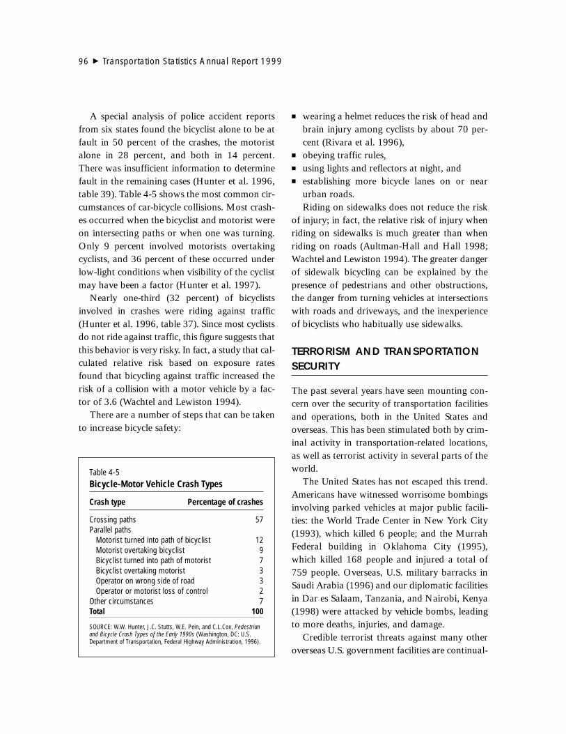
A special analysis of police accident reportsfrom six states found the bicyclist alone to be atfault in 50 percent of the crashes, the motoristalone in 28 percent, and both in 14 percent.There was insufficient information to determinefault in the remaining cases (Hunter et al. 1996,table 39). Table 4-5 shows the most common cir-cumstances of car-bicycle collisions. Most crash-es occurred when the bicyclist and motorist wereon intersecting paths or when one was turning.Only 9 percent involved motorists overtakingcyclists, and 36 percent of these occurred underlow-light conditions when visibility of the cyclistmay have been a factor (Hunter et al. 1997).
Nearly one-third (32 percent) of bicyclistsinvolved in crashes were riding against traffic(Hunter et al. 1996, table 37). Since most cyclistsdo not ride against traffic, this figure suggests thatthis behavior is very risky. In fact, a study that cal-culated relative risk based on exposure ratesfound that bicycling against traffic increased therisk of a collision with a motor vehicle by a fac-tor of 3.6 (Wachtel and Lewiston 1994).
There are a number of steps that can be takento increase bicycle safety:
� wearing a helmet reduces the risk of head andbrain injury among cyclists by about 70 per-cent (Rivara et al. 1996),
� obeying traffic rules,� using lights and reflectors at night, and� establishing more bicycle lanes on or near
urban roads.Riding on sidewalks does not reduce the risk
of injury; in fact, the relative risk of injury whenriding on sidewalks is much greater than whenriding on roads (Aultman-Hall and Hall 1998;Wachtel and Lewiston 1994). The greater dangerof sidewalk bicycling can be explained by thepresence of pedestrians and other obstructions,the danger from turning vehicles at intersectionswith roads and driveways, and the inexperienceof bicyclists who habitually use sidewalks.
TERRORISM AND TRANSPORTATIONSECURITY
The past several years have seen mounting con-cern over the security of transportation facilitiesand operations, both in the United States andoverseas. This has been stimulated both by crim-inal activity in transportation-related locations,as well as terrorist activity in several parts of theworld.
The United States has not escaped this trend.Americans have witnessed worrisome bombingsinvolving parked vehicles at major public facili-ties: the World Trade Center in New York City(1993), which killed 6 people; and the MurrahFederal building in Oklahoma City (1995),which killed 168 people and injured a total of759 people. Overseas, U.S. military barracks inSaudi Arabia (1996) and our diplomatic facilitiesin Dar es Salaam, Tanzania, and Nairobi, Kenya(1998) were attacked by vehicle bombs, leadingto more deaths, injuries, and damage.
Credible terrorist threats against many otheroverseas U.S. government facilities are continual-
96 � Transportation Statistics Annual Report 1999
Table 4-5Bicycle-Motor Vehicle Crash Types
Crash type Percentage of crashes
Crossing paths 57Parallel paths
Motorist turned into path of bicyclist 12Motorist overtaking bicyclist 9Bicyclist turned into path of motorist 7Bicyclist overtaking motorist 3Operator on wrong side of road 3Operator or motorist loss of control 2
Other circumstances 7Total 100
SOURCE: W.W. Hunter, J.C. Stutts, W.E. Pein, and C.L.Cox, Pedestrianand Bicycle Crash Types of the Early 1990s (Washington, DC: U.S.Department of Transportation, Federal Highway Administration, 1996).

ly being identified and evaluated, and trans-portation-related attacks have occurred in othernations. These include the release of sarin nervegas in the Tokyo subway system (1998), as wellas assaults against transit vehicles and systems inFrance, Israel, China, and several LatinAmerican nations.
The State Department’s Office of theCoordinator for Counter-Terrorism issues anannual report on Patterns of Global Terrorism(USDOS 1999). In recent years, the incidence ofinternational terrorism has fluctuated greatly.Although the number of incidents has remainedrelatively constant at about 300 to 400 annually,the casualties resulting from these events havevaried widely from under 1,000 to nearly 7,000(see table 4-6). A single incident can range fromthe attempted kidnapping of an individual to amassive bombing of a public facility with numer-ous casualties and significant destruction.
The most recent report lists 273 acts of inter-national terrorism in 1998, a decrease of 31from 1997. However, these attacks resulted inthe largest number of casualties—741 deathsand 5,952 injuries for a total of 6,693—in anyyear on record. More than 5,500 casualties wererelated to the bombings of the U.S. embassies inNairobi and Dar es Salaam. The 12 U.S. citizenswho died in the Nairobi incident were the onlyAmericans to lose their lives to terrorism in1998. About 40 percent of the 1998 incidents—
or 111 of the 273 events—involved U.S. targets.Most of these were bombings of U.S. oil compa-ny pipelines in Colombia.
According to DOT’s Federal Aviation Ad-ministration, there were 216 criminal incidentsinvolving attacks against civil aviation aroundthe world from 1993 through 1997. About 40percent of the incidents (87) involved hijackings.Another 50 involved attacks at airports, and 32involved attacks at off-airport facilities (USDOTFAA 1997).
Several recent initiatives by Congress and theExecutive Branch emphasized security issues. In1997, the Commission on Aviation Safety andSecurity recommended 77 improvements in avi-ation safety, security, disaster response, and airtraffic control (USEOP 1997). Agencies respon-sible for implementing these recommendationsare the Departments of Defense, State, andTransportation; the Federal Bureau of Investiga-tion; the National Transportation Safety Board;the U.S. Customs and Postal Services; and theBureau of Alcohol, Tobacco and Firearms.4
In July 1996, Executive Order 13010 estab-lished the President’s Commission on CriticalInfrastructure Protection (PCCIP). PCCIP con-ducted a comprehensive review of both the phys-ical and electronic, or “cyber,” vulnerabilities offive of the nation’s critical infrastructure sectors,defined as systems that, if damaged or disrupted,would have serious negative consequences toeconomic activities or national security. Thesefive sectors were: information and communica-tions; banking and finance; energy, includingelectrical power, oil, and gas; vital human ser-vices, such as emergency medical response; andphysical distribution, including transportation asits major component.
Chapter 4 Transportation Safety � 97
Table 4-6International Terrorist Incidents andCasualties: 1993–98
Year 1993 1994 1995 1996 1997 1998
Incidents 431 322 440 296 304 273Casualties 1,510 988 6,454 3,225 914 6,693
SOURCE: U.S. Department of State, Patterns of Global Terrorism, 1998(Washington, DC: 1999), appendix C.
4 DOT’s annual status report (USDOT 1998) on the imple-mentation progress is available on the Internet at www.dot.gov/affairs/whcoasas.htm.

PCCIP’s report, issued in October 1997(USEOP 1997) contained recommendations toimprove the nation’s response capability. PCCIPidentified three areas where transportation waspotentially vulnerable. The first would exist ifthe satellite-based Global Positioning Systembecame the sole source for radionavigation foraircraft landings by the year 2010, as scheduled.The second is related to vulnerabilities as a resultof the modernization of the National AirspaceSystem. The third concern arises from the poten-tial vulnerability of advanced electronic informa-tion and communications systems usedthroughout the transportation system. For exam-ple, disruptions in computer-based systems usedin pipeline operations to monitor flow and pres-sure and issue automatic electronic commands toremote pumping stations and valves could leadto pipeline failures, environmental damage, andsupply shortages. In May 1998, PresidentialDecision Directive (PDD) 62 on CombatingTerrorism (USEOP 1998a) and PDD 63 on Pro-tecting America’s Critical Infrastructure (USEOP1998b) established a number of new interagencyorganizations to oversee the implementation ofthe PCCIP recommendations.
INTERNATIONAL TRENDS INROAD SAFETY
Long the dominant mode of travel in the UnitedStates, motor vehicles are becoming a preferredmeans of transportation both in other industrial-ized countries and in the developing world. InWestern Europe, despite its extensive and well-traveled transit and rail networks, automobilesaccount for more than 86 percent of passenger-kilometers traveled (ECMT 1998).
In 1996, more than 671 million vehicles wereregistered in the world, up from 411 million in1980. Although the United States has the mostvehicles by far, well over 200 million, its share of
the world total declined from 44 percent in 1970to 31 percent in 1995 (AAMA 1994; 1998). As fig-ure 4-6 shows, in 1960 there were 100 million pas-senger cars registered in the world; by 1995, therewere 480 million. Proportionally, the growth incommercial vehicles was even greater, growingfrom 30 million in 1960 to 170 million in 1995.
World Motor Vehicle FatalitiesData on the number of fatalities and injuriesinvolving motor vehicle crashes worldwide arelimited. Britain’s Transport and Road ResearchLaboratory (TRRL) estimates that 300,000 per-sons die and 10 million to 15 million persons areinjured each year in road crashes around theworld (TRRL 1991). Other estimates are higher.One estimate, cited by the InternationalFederation of Red Cross and Red CrescentSocieties, is that 500,000 people died in trafficcrashes in 1990, and 15 million were injuredworldwide (IFRC 1998, 20). According to theWorld Health Organization (WHO), road trafficaccidents in 1998 were the largest cause of ill
98 � Transportation Statistics Annual Report 1999
1960 1965 1970 1975 1980 1985 1990 19950
50
100
150
200
250
300
350
400
450
500
Passenger cars
Commercial vehicles
Vehicle registrations (millions)
Figure 4-6World Motor Vehicle Registration Trends: 1960–95
SOURCES: American Automobile Manufacturers Association, World MotorVehicle Data (Washington, DC: 1994).
________. Motor Vehicle Facts & Figures, 1998 (Washington, DC: 1998).

health or early death for males between the agesof 15 and 44 worldwide, and the second largestcause in developing countries. WHO warnedthat the burden from traffic accidents wouldlikely increase, especially in developing countries(WHO 1999, 17–18).
Although some countries have made greatstrides in recent years to reduce vehicle-relateddeaths and injuries, in others, the number of vehi-cles is growing far faster than the physical, legal,and institutional infrastructure needed to safelyaccommodate them. Table 4-7 shows the numberof motor vehicle fatalities in selected countries in1980 and 1996. Most of the countries cited in thetable had fewer fatalities in 1996 than 16 yearsearlier. Many of these countries improved motorvehicle safety through better road design, plan-ning, and operations. Conversely, countries witha greater number of deaths in 1996 are generallythose in which vehicle use has risen both quicklyand relatively recently.
Safety Issues in Developing CountriesWhile road safety in most industrialized coun-tries is improving, for many newly developed ordeveloping nations safety problems are worsen-ing. For example, between 1968 and 1985, thenumber of motor vehicle fatalities in someAfrican countries rose by more than 300 percentand in Asian countries by over 170 percent. Inthat same period, the number of motor vehiclefatalities in industrialized countries decreased by25 percent (TRRL 1991).
According to Britain’s TRRL, growth inmotorization and urbanization in emerging anddeveloping nations has increased traffic on roadsthat were never designed to carry the volumesthat they do today. Moreover, unplanned growthhas led to incompatible land use in sprawlingurban areas and created significant driving haz-ards. In many countries, poor road conditions,badly designed intersections, and inadequate
Chapter 4 Transportation Safety � 99
Table 4-7Motor Vehicle Fatalities in SelectedCountries: 1980 and 1996(Thousands)
Country 1980 1996
Australia 3.27 1.97Austria 2.00 1.03Belgium 2.40 1.36Denmark 0.69 0.51Egypt N a4.40
Finland 0.55 0.40France 13.67 8.54Hong Kong 0.46 0.26Hungary 1.63 1.11Iceland 0.03 0.01
Ireland 0.56 0.45Israel 0.40 0.52Japan 11.39 11.67Kenya N b2.67Korea, Republic of 6.45 10.09
Morocco c3.52 2.81Netherlands 1.97 1.18New Zealand 0.60 0.58Norway 0.36 0.26Oman c0.47 0.51
Portugal 2.94 2.08Senegald 0.47 0.79Spain 6.52 5.48Sri Lanka 0.63 e1.92Sweden 0.85 0.57
Switzerland 1.21 0.62Taiwan c2.72 2.99Turkey c6.19 5.43United Kingdom 6.24 3.74United States 51.10 42.07a Data are for 1994. d Data are for 1992 and 1995.b Data are for 1992. e Data are for 1995.c Data are for 1982.
KEY: N = data are nonexistent; OECD = Organization for EconomicCooperation and Development.
NOTE: Not all countries adhere to the rule that counts deaths occurringwithin 30 days of an event; data for the United States and OECD coun-tries are harmonized.
SOURCES:International Road Federation, World Road Statistics (Geneva, Switzer-land: 1998).National Safety Council, International Accident Facts (Itasca, IL: 1995).Organization for Economic Cooperation and Development, InternationalRoad Traffic and Accident Database, 1998, available at www.bast.de/irtad.U.S.Department of Transportation, National Highway Traffic SafetyAdministration, Traffic Safety Facts 1997 (Washington, DC: 1998).

protection have exacerbated these dangers forpedestrians (TRRL 1991).
TRRL identifies at least four conditions con-tributing to road safety problems in developingcountries:� Inadequate design standards. In many devel-
oping countries, highway design standards areeither outdated (sometimes going back tocolonial times) or inappropriate (usuallybecause standards in industrialized countriesare applied without considering local needs).Such standards may ignore pedestrians orother nonmotorized transportation or may betoo costly for countries to afford.
� Limited resources. Developing nations oftenlack the engineers and other professionals, aswell as the financial resources, needed tomodify design standards to accommodatelocal conditions or to properly maintain roadsand other infrastructure.
� Operational and control deficiencies. Opera-tional practices have not kept pace with roadbuilding in the developing world. For exam-ple, roads are often poorly maintained, trafficsignage may be inadequate, walkways forpedestrians are often nonexistent or in poorcondition, and control measures to channelvehicles are rarely available (TRRL 1991, 4).
� Inadequate driver training. Drivers in develop-ing countries typically lack the experience oftheir counterparts in the industrialized world.Many such drivers have never been adequate-ly tested or trained. Moreover, enforcement oftraffic laws in developing countries is oftenineffective and driver compliance poor.Safety improvements implemented in the
industrialized world have the potential to signifi-cantly reduce road hazards in less developednations. According to TRRL, among the mostsuccessful strategies are more safety-consciousroad planning and elimination of hazardous loca-tions on roadways through traffic engineering.
DATA NEEDS
While a great deal is known about transporta-tion accidents and incidents and the resultingfatalities, injuries, and property damage, there ismuch that is not known. This section brieflydescribes areas where the data available at pre-sent are insufficient.
Safety data are, broadly speaking, of twotypes: outcome data, such as numbers of acci-dents, fatalities, and injuries; and exposure data,typically expressed as vehicle-miles, passenger-miles, or aircraft departures. The latter are tradi-tionally harder to collect. The following is a listof major exposure data needs:� exposure measures for the commercial water-
borne mode and for pipelines;� a better exposure measure for recreational
boating and better estimates of the number ofregistered boats;
� data separated by air taxi and general aviationexposures (number of landings), as these dataare available only in a combined form since1994;
� because the common exposure measure forthe highway mode, vehicle-miles traveled(vmt), is derived from a sample, error bars onvmt would be very useful in interpreting fatal-ity and crash rates; and
� measures of exposure of specific populations(e.g., elderly drivers or children) and exposureto specific conditions (e.g., adverse weather)are not available, particularly for the highwaymode.Some outcome data are also either not avail-
able, or available in combination with fatalities,injuries, and incidents, which are not strictlytransportation-related. Some of these data needsare:� transit and rail fatalities presented in a clear,
easy-to-understand format, distinguishingoccupants from nonoccupants, and trans-
100 � Transportation Statistics Annual Report 1999

portation incidents (e.g., collisions and derail-ments) from nontransportation incidents (e.g.,homicides).
� property damage from highway crashes.
REFERENCES
American Automobile Manufacturers Associ-ation (AAMA). 1994. World Motor VehicleData. Washington, DC.
_____. 1998. Motor Vehicle Facts & Figures,1998. Washington, DC.
Aultman-Hall, L. and F.L. Hall. 1998. Ottawa-Carleton Commuter Cyclist On- and Off-Road Incident Rates. Accident Analysis andPrevention 30, no. 1:29–43.
European Conference of Ministers of Transport(ECMT). 1998. Trends in the TransportSector 1970–1996. Paris, France: OECDPublications Service.
Hunter, W.W., J.C. Stutts, and W.E. Pein. 1997.Bicycle Crash Types: A 1990’s InformationalGuide, FHWA-RD-96-104. Washington, DC:U.S. Department of Transportation, FederalHighway Administration.
Hunter, W.W., J.C. Stutts, W.E. Pein, and C.L.Cox. 1996. Pedestrian and Bicycle CrashTypes of the Early 1990s. Washington, DC:U.S. Department of Transportation, FederalHighway Administration.
International Federation of Red Cross and RedCrescent Societies (IFRC). 1998. WorldDisasters Report 1998. Geneva, Switzerland.
Joksch, H. 1998. Fatality Risks in CollisionsBetween Cars and Light Trucks, DOT/HS-808-802, prepared for the U.S. Department ofTransportation, National Highway TrafficSafety Administration. University of MichiganTransportation Research Institute. October.
National Association of State Directors of PupilTransportation Services (NASDPTS). n.d.
Passenger Vans Used as School Buses, positionpaper. Available at www.stnonline.com/core2_files/bbs/nasdpts/sd_pp1.htm.
National School Transportation Association(NSTA). 1999. NSTA Transportation Survey.Available at www.stnonline.com/core2_files/statistics/vans11ormore.htm.
National Transportation Safety Board (NTSB).1987. Crashworthiness of Large PoststandardSchool Buses, Report No. NTSB/SS-87/01.Available at www.stnonline.com/core2_files/bbs/ntsb/largebusstudy.htm.
_____. 1997. Highway Accident/Incident Sum-mary Report: Collision with a Pedestrian by aUtility Truck Near Cosmopolis, Washington,November 26, 1996, Report No. NTSB/HAR-97/01/SUM. Washington, DC.
Pickrell, D. and P. Schimek. 1997. Trends inPersonal Motor Vehicle Ownership and Use:Evidence from the Nationwide PersonalTransportation Survey. Washington, DC: U.S.Department of Transportation, FederalHighway Administration. Also available atwww-cta.ornl.gov/npts/1995/Doc/publica-tions.shtml.
Rivara, F.P., D.C. Thompson, and R.S. Thomp-son. 1996. Circumstances and Severity ofBicycle Injuries. Seattle, WA: Snell MemorialFoundation, Harborview Injury Preventionand Research Center.
Tinsworth, D., C. Polen, and S. Cassidy. 1993.Bicycle-Related Injuries: Injury, Hazard, andRisk Patterns, Technical Report. Washington,DC: U.S. Consumer Product Safety Com-mission.
Transportation Research Board (TRB), NationalResearch Council. 1989. Improving SchoolBus Safety, Special Report 222. Washington,DC.
Chapter 4 Transportation Safety � 101

Transport and Road Research Laboratory(TRRL), Overseas Development Administra-tion. 1991. Towards Safer Roads in De-veloping Countries: A Guide for Planners andEngineers. United Kingdom: Ross SilcockPartnership.
U.S. Department of State (USDOS). 1999.Patterns of Global Terrorism: 1998, Pub-lication 10610. Washington, DC. April.
U.S. Department of Transportation (USDOT).1998. White House Commission on AviationSafety and Security: The DOT Status Report.Available at www.dot.gov/affairs/whcoasas.htm,as of 7 June 1999.
U.S. Department of Transportation (USDOT),Federal Aviation Administration (FAA). 1997.Criminal Acts Against Civil Aviation.Available at http://cas.faa.gov/cas/crim97.htm.
U.S. Department of Transportation (USDOT),National Highway Traffic Safety Administra-tion (NHTSA). 1997. Fatality AnalysisReporting System. Available at www.fars.nhtsa.dot.gov.
_____. 1998a. School Bus Safety: Safe Passagefor America’s Children. Available at www.nhtsa.dot.gov/people/injury/buses/schbus/schbussafe.html.
_____. 1998b. Traffic Safety Facts 1997.Available at www.nhtsa.dot.gov/people/ncsa/TSF97.html.
____.1998c. Traffic Safety Facts 1997: LargeTrucks. Available at www.nhtsa.dot.gov/people/ncsa/Truck97.html.
_____. 1998d. Traffic Safety Facts 1997: Pedal-cyclists. Available at www.nhtsa. dot.gov/people/ncsa/PedCycle97.html.
_____. 1998e. Traffic Safety Facts 1997:Pedestrians. Available at www.nhtsa.dot.gov/people/ncsa/Ped97.html.
_____. 1998f. Traffic Safety Facts 1997: SchoolBuses. Available at www.nhtsa.dot.gov/people/ncsa/factshet.html.
____. 1999. Traffic Safety Facts: Overview 1998.Available at www.nhtsa.dot.gov/people/ncsa/factsheet.html
U.S. Executive Office of the President (USEOP).1997. Final Report of the White HouseCommission on Aviation Safety and Security.Washington, DC. February.
____. 1998a. Presidential Decision Directive 63:Combating Terrorism, Fact Sheet. Washing-ton, DC. May.
____. 1998b. Presidential Decision Directive 62:Protecting America’s Critical Infrastructure,Fact Sheet. Washington, DC. May.
Wachtel, A. and D. Lewiston. 1994. Risk Factorsfor Bicycle-Motor Vehicle Collisions atIntersections. ITE Journal. September.
World Health Organization (WHO). 1999.World Health Report 1999. Geneva,Switzerland.
102 � Transportation Statistics Annual Report 1999

Without energy, vehicles and other forms of transportation cannot move.The U.S. transportation sector requires great quantities of energy, abouta quarter of the national total. Petroleum supplies about 97 percent of
the energy used in transportation in the form of gasoline, diesel fuel, or other lightoils (USDOE 1998b). For more than a century, no other fuel has been able to com-pete successfully with petroleum for motorized transportation. Were it not for itsenvironmental impacts, petroleum’s portability (light weight and high energy con-tent) and ease of control make it a nearly ideal transportation fuel. The only othersignificant sources are natural gas, used to drive compressors on pipelines, electrici-ty for rails and subways, and alcohol for blending into gasoline.
Energy supply is not a problem at this time. Petroleum production capabilityworldwide is so much greater than demand that prices in 1998 reached virtually all-time lows (in real terms). Resource constraints that could lead to rising prices arethought to be at least a decade away, and possibly much further. Even U.S. produc-tion, which had been in a seemingly inexorable decline since 1970, has almost lev-eled out, despite low prices. The supply system works so effectively that even localdisruptions are rare except for occasional weather problems or natural disasters.
�
103
Transportation, Energy, and the Environment
chapter five

Nevertheless, serious energy and environmen-tal issues are associated with transportation. Thecurrent abundance of petroleum cannot beassured in the future. Over half the petroleumused in the United States must now be imported.Most U.S. imports are from suppliers who havebeen reliable, but political instability in any ofthe major producer regions could disrupt worldsupplies, leading to steep price increases, as hasoccurred several times since the early 1970s.Economic damage could be serious. TheStrategic Petroleum Reserve was established toprovide additional supplies when imports aredisrupted, but, as discussed below, its ability todo so is diminishing. The transportation sectoruses over 65 percent of all the petroleum con-sumed in this country (up from 60 percent in1975) (USDOE 1998b). The lack of significantalternatives leaves transportation particularlyvulnerable should a disruption occur in the sup-ply system.
Furthermore, heavy dependence on petroleumis the root of most environmental problemscaused by transportation. Despite majorimprovements in emission rates over the last twodecades, transportation continues to be the pri-mary source of pollutants that affect air quality:carbon monoxide, nitrogen oxides, and volatileorganic compounds. Fuel consumption bymobile sources also results in a large percentageof the key hazardous air pollutants released inurban and rural areas of the nation. Moreover,the transportation sector contributes to otherenvironmental impacts such as oil spills and haz-ardous waste. Upcoming federal efforts to reducethese impacts will influence technology andoperational changes across the sector.
In addition, the carbon dioxide (CO2) createdby combustion of petroleum in the transporta-tion sector is responsible for about 26 percent ofall greenhouse gases emitted in the United States,which in turn accounts for about one-quarter of
all anthropogenic emissions of greenhouse gasesin the world (USDOE 1998e). Mounting evi-dence shows that global climate change is poten-tially a very serious problem. If efforts to controlgreenhouse gas emissions are undertaken, overallcosts will be minimized if the lowest cost optionsare implemented. Each economic sector, includ-ing transportation, has potential low-cost reduc-tions.
This chapter describes the current status ofenergy and environmental issues. It also reviewsvarious technologies that could alleviate theproblems.
ENERGY 1
As the economy has grown, so has transporta-tion and the use of energy. There are, however,marked differences in the growth rates, as shownin figure 5-1. Energy use in the transportationsector has grown by a factor of about 2.34 since1960, less than passenger-miles, despite theincreased size of cars and engines now. Improvedvehicular efficiency is largely responsible for thisdifference, as discussed in the next section.Figure 5-2 shows energy consumption by modefor 1997. Total energy for transportation was24.8 quadrillion (quads) British thermal units(Btu). Highway vehicles account for about 80percent of total transportation energy use and 84percent of transportation petroleum consump-tion (USDOE 1998b and USDOT BTS Forth-coming).
104 � Transportation Statistics Annual Report 1999
1 Energy Information Administration (EIA) data are usedthroughout this chapter. EIA relies on surveys to collect itsenergy data and models to forecast energy supply anddemand. For information about survey methodology andstatistical reliability, the reader is referred to EIA referencescited in this chapter or the EIA website at www.eia.doe.gov.For information about EIA’s modeling standards, please seewww.eia.doe.gov/oss/standard.html.

Vehicle EconomyAutomobiles and other vehicles are far more effi-cient today than at the start of the energy crisisin 1973, and improvements are still being imple-mented. Manufacturers have reduced vehicleweight, improved the rolling resistance of tires,
and added lockup torque conversion to trans-missions to eliminate slippage at highway speeds.Engines have been improved by switching fromcarburetors to fuel injection, improving combus-tion control, and adding valves to improveengine breathing. Trucks as well as cars havebenefited from these improvements, but heavierframes and poorer aerodynamics mean thattrucks are necessarily less efficient.
Since 1988, however, essentially all the gain innew motor vehicle efficiency has been offset byincreases in weight and power within classes,and by consumer shifts to lower economy vehi-cles, especially light-duty trucks (sport utilityvehicles, minivans, and pickup trucks). Thesales-weighted average weight of new cars rosefrom 2,805 pounds in 1988 to 3,071 pounds in1997 (average weight was 3,349 pounds at thestart of fuel economy standards in 1978). Also,engines gained about 35 horsepower during thisperiod (USDOT NHTSA 1998).
Figure 5-3 shows the trends in fuel consump-tion for highway vehicles. It is clear from the
Chapter 5 Transportation, Energy, and the Environment � 105
0
1
2
3
4
5
6
7
8
Transportation energy, 10 quads
Passenger-miles, trillions
Real Gross Domestic Product (GDP), trillions of chained 1992 dollars
Population, 100s of millions
SOURCES: U.S. Department of Transportation, Bureau of Transportation Statistics, National Transportation Statistics 1999 (Washington, DC: Forth-coming); U.S. Department of Commerce, Bureau of Economic Analysis, Survey of Current Business, December 1998.
Figure 5-1Transportation Energy and Economic Activity: 1960–97
Growth factorsGDP = 3.21travel = 3.16energy = 2.34population = 1.49
1960 1962 1964 1966 1968 1970 1972 1974 1976 1978 1980 1982 1984 1986 1988 1990 1992 1994 1996
Figure 5-2Transportation Energy Use by Mode: 1997
SOURCE: U.S. Department of Transportation, Bureau of Trans-portation Statistics, National Transportation Statistics 1999(Washington, DC: Forthcoming).
Heavy-duty trucks and buses, 18%
Transit, 1%Rail, 2%
Water, 5%
Pipeline, 3%
Air, 8%
Cars and light-duty vehicles, 63%
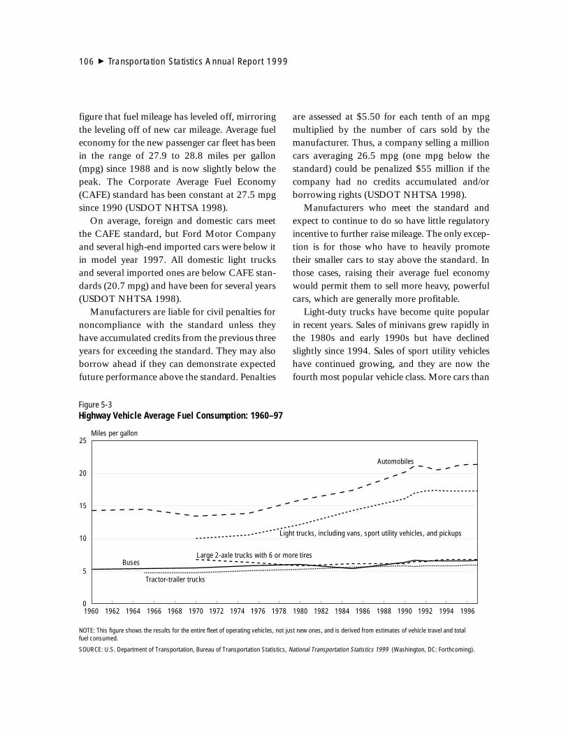
figure that fuel mileage has leveled off, mirroringthe leveling off of new car mileage. Average fueleconomy for the new passenger car fleet has beenin the range of 27.9 to 28.8 miles per gallon(mpg) since 1988 and is now slightly below thepeak. The Corporate Average Fuel Economy(CAFE) standard has been constant at 27.5 mpgsince 1990 (USDOT NHTSA 1998).
On average, foreign and domestic cars meetthe CAFE standard, but Ford Motor Companyand several high-end imported cars were below itin model year 1997. All domestic light trucksand several imported ones are below CAFE stan-dards (20.7 mpg) and have been for several years(USDOT NHTSA 1998).
Manufacturers are liable for civil penalties fornoncompliance with the standard unless theyhave accumulated credits from the previous threeyears for exceeding the standard. They may alsoborrow ahead if they can demonstrate expectedfuture performance above the standard. Penalties
are assessed at $5.50 for each tenth of an mpgmultiplied by the number of cars sold by themanufacturer. Thus, a company selling a millioncars averaging 26.5 mpg (one mpg below thestandard) could be penalized $55 million if thecompany had no credits accumulated and/orborrowing rights (USDOT NHTSA 1998).
Manufacturers who meet the standard andexpect to continue to do so have little regulatoryincentive to further raise mileage. The only excep-tion is for those who have to heavily promotetheir smaller cars to stay above the standard. Inthose cases, raising their average fuel economywould permit them to sell more heavy, powerfulcars, which are generally more profitable.
Light-duty trucks have become quite popularin recent years. Sales of minivans grew rapidly inthe 1980s and early 1990s but have declinedslightly since 1994. Sales of sport utility vehicleshave continued growing, and they are now thefourth most popular vehicle class. More cars than
106 � Transportation Statistics Annual Report 1999
Automobiles
Light trucks, including vans, sport utility vehicles, and pickups
Large 2-axle trucks with 6 or more tires
Tractor-trailer trucks
Buses
NOTE: This figure shows the results for the entire fleet of operating vehicles, not just new ones, and is derived from estimates of vehicle travel and total fuel consumed.
SOURCE: U.S. Department of Transportation, Bureau of Transportation Statistics, National Transportation Statistics 1999 (Washington, DC: Forthcoming).
Miles per gallon
Figure 5-3Highway Vehicle Average Fuel Consumption: 1960–97
1960 1962 1964 1966 1968 1970 1972 1974 1976 1978 1980 1982 1984 1986 1988 1990 1992 1994 19960
5
10
15
20
25

trucks are sold in this country, but the differenceis narrowing. In 1988, 10,370,000 cars and4,740,000 light trucks were sold; in 1997, therewere 8,260,000 cars and 6,530,000 trucks sold.Figure 5-4 shows sales of light vehicles by class(excluding classes of less than 100,000 sales).Sales of most light truck classes gained, whilemost automobile classes declined (Davis 1998).
Some of this trend may be short-term in dura-tion, but, clearly, many buyers are finding whatthey want in light trucks rather than cars: interi-or spaciousness, carrying capacity, visibility, anda perception of safety (at least for themselves ifnot for occupants of other cars in a collision.)However, the trend does have implications forenergy consumption because light trucks averageabout 5 mpg less than cars. Figure 5-5 shows thesales-weighted CAFE rating for the same classesof light vehicles, divided into those that increasedsales and those that lost sales from 1990 to1997. Only midsize cars gained in sales, and thatwas very slight. The biggest sales loser amongtrucks was the one with the highest mileage,small pickups. Overall, figure 5-5 shows amarked shift from high mileage to lower mileagevehicles.
A variety of technologies for further raisingefficiency are available or are emerging from thelaboratory. Improving aerodynamics to reducedrag is one of the most important in the nearterm. Internal engine improvements such as vari-able valve timing and lower rolling resistancetires can also be important. In the longer term,transmissions may have improved electroniccontrols to select the gear that will allow theengine to operate most efficiently for the givenload. A continuously variable transmissionwould be even better, allowing the engine tooperate at peak efficiency at all times. Theseimprovements, and more radical technologiessuch as the diesel hybrid engine or fuel cells,could be introduced by automobile manufactur-
ers if they saw sufficient demand or were in-duced by regulations.
Absent higher fuel prices or tightened regula-tions, however, these advances will be imple-mented slowly at best. Most manufacturers meetthe current standards, and consumers are notdemanding greatly increased economy. There-fore, petroleum consumption is likely to contin-ue to increase in the transportation sector.
Energy consumption per passenger-mile (energy intensity) for some other means of traveldiffers surprisingly little from automobiles. How-ever, intermodal comparisons should be consid-ered approximations. Data for the differentmodes are collected in a variety of ways and arebased on different assumptions. For example, air-lines record passenger-miles, but data on occu-pancy of private automobiles are estimated fromsurveys. Even relatively hard data, such as statesales of gasoline, must be modified to resolveanomalies, and transit data, which cover lightand heavy rail, are more difficult to reconcile.
With these caveats in mind, in 1996 passengercar energy intensity was about 3,700 Btu perpassenger-mile, down slightly from 3,900 in1990 and 4,200 in 1980. (Even though newvehicle fuel economy has leveled off, the entirefleet is still more efficient today than years ago,which indicates why energy intensity hasdeclined somewhat.) Light-truck energy intensitywas 4,529 Btu per passenger-mile in 1996, downfrom 4,859 in 1990 and 5,384 in 1980 (assum-ing the same occupancy rates as automobiles).Air carrier energy intensity was 4,100 Btu perpassenger-mile in 1996 (versus 4,800 in 1990and 5,800 in 1980) (Davis 1998). The decline inenergy intensity of air travel is due largely tohigher occupancy. Flying a full plane requiresconsiderably less than twice the fuel of a half-fullone, but yields twice the passenger-miles. Airlineshave been increasingly successful in filling theirplanes. Some have even reconfigured seating to
Chapter 5 Transportation, Energy, and the Environment � 107

108 � Transportation Statistics Annual Report 1999
0
1,000,000
2,000,000
3,000,000
4,000,000
5,000,000Subcompact car
1976 1980 1984 1988 1992 1996
Figure 5-4U.S. Sales of Domestic and Foreign Light-Duty Vehicles by Class
0
1,000,000
2,000,000
3,000,000
4,000,000
5,000,000Midsize car
1976 1980 1984 1988 1992 19960
1,000,000
2,000,000
3,000,000
4,000,000
5,000,000Compact car
1976 1980 1984 1988 1992 1996
0
1,000,000
2,000,000
3,000,000
4,000,000
5,000,000Large car
1976 1980 1984 1988 1992 19960
1,000,000
2,000,000
3,000,000
4,000,000
5,000,000Large pickup
1976 1980 1984 1988 1992 19960
1,000,000
2,000,000
3,000,000
4,000,000
5,000,000Small pickup
1976 1980 1984 1988 1992 1996
0
1,000,000
2,000,000
3,000,000
4,000,000
5,000,000Small van
1976 1980 1984 1988 1992 1996
0
1,000,000
2,000,000
3,000,000
4,000,000
5,000,000Large utility
1976 1980 1984 1988 1992 1996
0
1,000,000
2,000,000
3,000,000
4,000,000
5,000,000Small utility
1976 1980 1984 1988 1992 19960
1,000,000
2,000,000
3,000,000
4,000,000
5,000,000Large van
1976 1980 1984 1988 1992 1996
SOURCE: S.C. Davis, Transportation Energy Data Book, Edition 18, ORNL-6941 (Oak Ridge, TN: Oak Ridge National Laboratory, 1998).
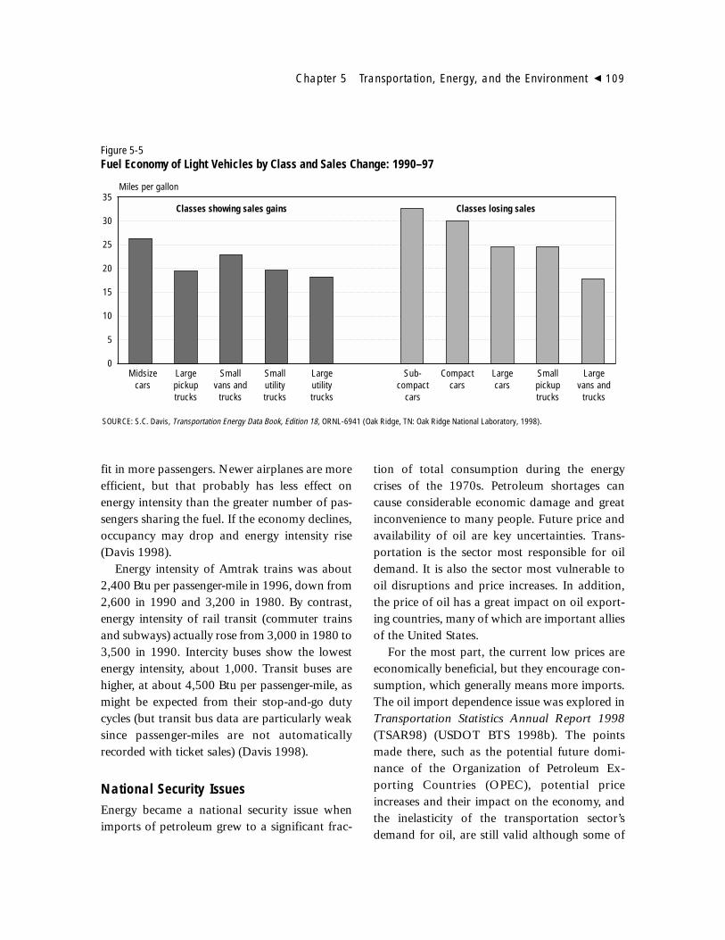
fit in more passengers. Newer airplanes are moreefficient, but that probably has less effect onenergy intensity than the greater number of pas-sengers sharing the fuel. If the economy declines,occupancy may drop and energy intensity rise(Davis 1998).
Energy intensity of Amtrak trains was about2,400 Btu per passenger-mile in 1996, down from2,600 in 1990 and 3,200 in 1980. By contrast,energy intensity of rail transit (commuter trainsand subways) actually rose from 3,000 in 1980 to3,500 in 1990. Intercity buses show the lowestenergy intensity, about 1,000. Transit buses arehigher, at about 4,500 Btu per passenger-mile, asmight be expected from their stop-and-go dutycycles (but transit bus data are particularly weaksince passenger-miles are not automaticallyrecorded with ticket sales) (Davis 1998).
National Security IssuesEnergy became a national security issue whenimports of petroleum grew to a significant frac-
tion of total consumption during the energycrises of the 1970s. Petroleum shortages cancause considerable economic damage and greatinconvenience to many people. Future price andavailability of oil are key uncertainties. Trans-portation is the sector most responsible for oildemand. It is also the sector most vulnerable tooil disruptions and price increases. In addition,the price of oil has a great impact on oil export-ing countries, many of which are important alliesof the United States.
For the most part, the current low prices areeconomically beneficial, but they encourage con-sumption, which generally means more imports.The oil import dependence issue was explored inTransportation Statistics Annual Report 1998(TSAR98) (USDOT BTS 1998b). The pointsmade there, such as the potential future domi-nance of the Organization of Petroleum Ex-porting Countries (OPEC), potential priceincreases and their impact on the economy, andthe inelasticity of the transportation sector’sdemand for oil, are still valid although some of
Chapter 5 Transportation, Energy, and the Environment � 109
0
5
10
15
20
25
30
35
Midsizecars
Classes showing sales gains Classes losing sales
Largepickuptrucks
Smallvans and
trucks
Smallutilitytrucks
Largeutilitytrucks
Sub-compact
cars
Compactcars
Largecars
Smallpickuptrucks
Largevans and
trucks
SOURCE: S.C. Davis, Transportation Energy Data Book, Edition 18, ORNL-6941 (Oak Ridge, TN: Oak Ridge National Laboratory, 1998).
Miles per gallon
Figure 5-5Fuel Economy of Light Vehicles by Class and Sales Change: 1990–97

the concerns seem far in the future. Moreover,some threats are difficult to foresee. Politicalproblems can arise even with countries withwhich the United States currently has stable rela-tions. For example, Venezuela is the largest sup-plier of oil to the United States, with 17 percentof all imports. The recently elected President ofVenezuela has expressed concern over its highlevel of exports, especially when the price is solow. Persian Gulf nations supply another 18 per-cent of imports, and all members of OPEC sup-ply 45 percent (USDOE 1998b).
The volume of imported oil and petroleumproducts surpassed that of U.S. production in1997, as shown in figure 5-6. In terms of energyvalue, imported petroleum exceeded domesticproduction in 1994, and has taken an increasedshare every year since. In 1997, the United Statesproduced 16.2 quadrillion Btu (quads) of petro-leum, including crude oil, natural gas plant, andother liquids. Net imports of crude oil and petro-leum products totaled 19.6 quads (USDOE1999). The transportation sector required 24quads of petroleum, equivalent to all U.S. pro-
duction plus 40 percent of all imports (USDOE1998b).
Never before in U.S. history, even at the heightof concern over energy in the 1970s, haveimports of petroleum exceeded production. U.Sproduction may stay level for a period or evenincrease slightly, but growth in demand basicallymeans growth in imports. When world oil sup-plies tighten, the United States could be morevulnerable to disruptions than ever before.
The Strategic Petroleum Reserve was createdin 1977 to help the country ride out disruptions.The size of the storage has stayed roughly con-stant since 1988, but imports have risen signifi-cantly. Therefore, the protection provided hasdropped steadily. In 1977, it held 563 millionbarrels, equivalent to 63 days of imports. Thepeak, in 1985, was 115 days (USDOE 1998b).
It is very unlikely that a high fraction of U.S.imports would be disrupted, but the Reserve isintended to protect against price shocks as wellas physical shortages. The transportation sector,with its relatively inelastic demand, would not beable to quickly reduce consumption by morethan a few percent without seriously inconve-niencing many people. If just 20 percent ofimports had to be replaced, the Reserve wouldlast about 10.5 months at current levels. Whilethat is more than supplied by any one country,petroleum exporting countries could well useany sizable disruption in world supplies to fur-ther restrict exports and raise prices.
The situation now is the exact opposite of thispotential problem. Asian economic difficultieshave reduced world oil demand appreciably,lowering prices and causing serious problems foroil producers. The Russian economy has beenparticularly hurt by the drop in revenues becauseoil is by far its most important export.
Oil prices are unlikely to rise very much untilAsian economies improve. Figure 5-7 shows pastoil price trends. Prior to the economic crises, oil
110 � Transportation Statistics Annual Report 1999
0
2,000
4,000
6,000
8,000
10,000
12,000
Total domestic production
Net imports
Barrels per day (thousands)
Figure 5-6Petroleum Production and Imports: 1980–98
SOURCE: U.S. Department of Energy, Energy Information Administration,Monthly Energy Review (Washington, DC: January 1999), tables 3.1a and b.
1980 1982 1984 1986 1988 1990 1992 1994 1996 1998

demand for 10 East Asian countries (Indonesia,South Korea, Thailand, Malaysia, Philippines,Singapore, Taiwan, Japan, China, and India) hadbeen growing at 5.6 percent per year, the fastestgrowth of any large region of the world. In 1998,East Asian oil demand was essentially un-changed, and world oil demand growth from1997 to 1998 was about 300,000 barrels perday. This is 25 percent lower than the 1.2 millionbarrels per day that the Energy InformationAdministration (EIA) had forecast before the cri-sis, even with low prices encouraging consump-tion in other importing countries (USDOE1998c).
It is unclear how quickly the East Asianeconomies will recover. Quite likely the recoveryschedule will be different for the various coun-tries, particularly since Japan’s problems are dif-ferent from the others. Japan is taking someimportant steps to stabilize its banks and restoreeconomic growth, but some analysts are skepti-cal that its efforts will be adequate. Other Asiancountries are showing signs of a turnaround, butit is too soon to tell if a recovery is underway.
Asian problems could contribute to soft oilprices for several years. Recently, EIA lowered itsprojected price of oil by about $5 per barrel forthe next several years (USDOE 1998c).
Alternative FuelsPetroleum provides about 97 percent of all trans-portation energy as shown in table 5-1. In 1992,it provided about 98 percent. The use of alterna-tive and replacement fuels doubled from 1992 to1998 while the use of gasoline rose only 10 per-cent, but that 10 percent increase (11.3 billiongallons) was more than twice as large as theentire use of alternative fuels (about 4.3 billiongallons) in 1998 (USDOE 1998a).
Nevertheless, there is considerable interest inalternative fuels for two reasons—reducing airemissions and oil dependence. TSAR98 dis-cussed the use of blending alternatives such asethyl alcohol (ethanol) and methyl-tertiary-butyl-ether (MTBE) with gasoline to reduceemissions. MTBE and ethanol, which is mixedwith gasoline to form gasohol, are oxygenates,which improve the combustion of gasoline. Theyare called replacement fuels because they direct-ly replace some gasoline out of each gallon thatconsumers buy. This application accounts formost of the nonpetroleum fuel used. Replace-ment fuels also slightly reduce carbon emissionsand oil consumption, as discussed elsewhere inthis chapter, but the main incentive for usingthem is to reduce local air pollution.
In theory, alternative fuels have far greaterpotential than replacement fuels to reduce oilconsumption, because they can replace all oralmost all the petroleum-based fuel that a vehicleuses, rather than the few percent that oxygenatesreplace. There are a variety of options for alter-native fuels. Of the 418,000 alternative-fueledvehicles (AFVs) operating in 1998, 274,000(about two-thirds) used liquefied petroleum gas(LPG), primarily propane (USDOE 1998a). LPG
Chapter 5 Transportation, Energy, and the Environment � 111
0
10
20
30
40
50
60
Chained 1992 dollars
Current dollars
1980 1982 1984 1986 1988 1990 1992 1994 1996 1998
Dollars per barrel
Figure 5-7World Oil Price: 1980–98
SOURCE: U.S. Department of Energy, Energy Information Administration,Annual Review of Energy 1998, DOE/EIA-0384(98) (Washington, DC:July 1999), table 5.19.
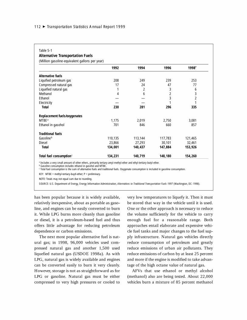
has been popular because it is widely available,relatively inexpensive, about as portable as gaso-line, and engines can be easily converted to burnit. While LPG burns more cleanly than gasolineor diesel, it is a petroleum-based fuel and thusoffers little advantage for reducing petroleumdependence or carbon emissions.
The next most popular alternative fuel is nat-ural gas; in 1998, 96,000 vehicles used com-pressed natural gas and another 1,500 usedliquefied natural gas (USDOE 1998a). As withLPG, natural gas is widely available and enginescan be converted easily to burn it very cleanly.However, storage is not as straightforward as forLPG or gasoline. Natural gas must be eithercompressed to very high pressures or cooled to
very low temperatures to liquefy it. Then it mustbe stored that way in the vehicle until it is used.One or the other approach is necessary to reducethe volume sufficiently for the vehicle to carryenough fuel for a reasonable range. Bothapproaches entail elaborate and expensive vehi-cle fuel tanks and major changes to the fuel sup-ply infrastructure. Natural gas vehicles directlyreduce consumption of petroleum and greatlyreduce emissions of urban air pollutants. Theyreduce emissions of carbon by at least 25 percentand more if the engine is modified to take advan-tage of the high octane value of natural gas.
AFVs that use ethanol or methyl alcohol(methanol) also are being tested. About 22,000vehicles burn a mixture of 85 percent methanol
112 � Transportation Statistics Annual Report 1999
Table 5-1Alternative Transportation Fuels(Million gasoline-equivalent gallons per year)
1992 1994 1996 1998P
Alternative fuelsLiquified petroleum gas 208 249 239 253Compressed natural gas 17 24 47 77Liquefied natural gas 1 2 3 6Methanol 4 6 2 3Ethanol — — 3 2Electricity — — 1 1
Total 230 281 296 335
Replacement fuels/oxygenatesMTBEa 1,175 2,019 2,750 3,081Ethanol in gasohol 701 846 660 857
Traditional fuelsGasolineb 110,135 113,144 117,783 121,465Diesel 23,866 27,293 30,101 32,461
Total 134,001 140,437 147,884 153,926
Total fuel consumption c 134,231 140,719 148,180 154,260a Includes a very small amount of other ethers, primarily tertiary-amyl-methyl-ether and ethyl-tertiary-butyl-ether.b Gasoline consumption includes ethanol in gasohol and MTBE.c Total fuel consumption is the sum of alternative fuels and traditional fuels. Oxygenate consumption is included in gasoline consumption.
KEY: MTBE = methyl-tertiary-buytl-ether; P = preliminary.
NOTE: Totals may not equal sum due to rounding.
SOURCE: U.S. Department of Energy, Energy Information Administration, Alternatives to Traditional Transportation Fuels 1997 (Washington, DC: 1998).

and 15 percent gasoline. A few hundred moreburn pure methanol, but these vehicles can bedifficult to start, especially in cold weather.Another 18,000 burn ethanol, usually with 15percent gasoline (USDOE 1998a).
Some vehicles are designed as flexible-fuelvehicles, capable of burning either alcohol orgasoline. Alcohol-fueled vehicles still use thebasic automobile engine but require substantialmodification to it. They will require radicalchanges to the fuel supply system if many ofthem are to operate. Methanol usually is pro-duced from natural gas but is much moreportable. Thus, it solves the storage problem fornatural gas but entails much more difficultproduction and distribution problems. Ethanolusually is made from grain using an energy-intensive process. Currently, ethanol does notoffer major petroleum-reduction or carbon diox-ide-reduction advantages because fossil fuels aretypically used to produce ethanol. Moreover,CO2 is produced in the fermentation process.
Advanced technologies, however, could allowalcohol to be produced much less expensivelyfrom renewable, nonfood sources such as woodand plant wastes. If successful, alcohol-fueledvehicles could contribute significantly to reducedpetroleum dependence, local air pollution, andcarbon dioxide emissions. Raising crops for theproduction of alcohol could slow the conversionof marginal farmland to forest, which would begood for farmers but might create some negativeenvironmental impacts, depending on the cropsraised and the land used. In fact, a farming resur-gence could reduce the credit the United States isexpected to receive for sequestration of carbon intrees, which is discussed below.
Yet another option is electric vehicles (EVs),the ultimate in flexible-fuel vehicles, because elec-tricity used to charge the batteries can be pro-duced from almost any energy source. These areconsidered to be the only zero-emissions vehicles
(ZEVs) because they do not burn any fuel them-selves. Some pollution may be produced whilegenerating power to charge the batteries, but netpollution from EVs frequently will be lower thanfrom conventional vehicles. If the power is gener-ated from renewable energy or nuclear power-plants, air pollution is negligible.
There are still many uncertainties over the fullenvironmental impact of the entire fuel cycle forboth conventional and electric vehicles. The rel-ative advantage of each will vary in differentparts of the country. At present, batteries are theonly means of storage, and they hold much lessenergy than the same volume of liquid fuels. Asa result, EV performance is distinctly inferior toconventional vehicles. They have a range ofabout 100 miles on today’s battery technologyand require lengthy recharging periods.Emerging technology (e.g., nickel-metal hydride)promises to be much better than lead-acid bat-teries. Several manufacturers now are offeringEVs with nickel-metal batteries. EVs can offermajor advantages in carbon reduction and oilindependence as well as reduced urban air pollu-tion if the technological problems can be solved.
Only about 6,000 EVs are currently operatingin the United States (USDOE 1998a). However,this number could rise rapidly. California andNew York have aggressively promoted the use ofEVs because of severe urban air pollution prob-lems. Both states were to have required automo-bile manufacturers to introduce ZEVs in 1998,but both programs have been postponed.California has reached an agreement with man-ufacturers that 10 percent of the new vehiclessold in the state in 2003 will be ZEVs. Manu-facturers hope that by then the technology, par-ticularly batteries, will have improved to thepoint that EVs will be sufficiently attractive thatpeople will want them. New York’s intendedrequirement of 2 percent of all cars sold in thestate in 1998 to be ZEVs was overturned by the
Chapter 5 Transportation, Energy, and the Environment � 113

Circuit U.S. Court of Appeals in August 1998 onthe grounds that it was preempted by the federalClean Air Act (EV World 1998).
GREENHOUSE GASES
Controlling the emissions of greenhouse gases,which most scientists believe could cause globalclimate change with a potentially disastrousimpact, is a contentious and complex issue forthe international community. Nevertheless, inter-national agreements to lessen the risk exist: � In 1992, the United Nations Framework Con-
vention on Climate Change, in Rio de Janeiro,established the principle that nations shouldtake voluntary steps to reduce emissions.
� In 1997, parties to the Convention met inKyoto, and agreed to a Protocol setting tar-gets for individual industrialized countries.
� The 1998 meeting of the parties in BuenosAires adopted a plan of action to resolve by2000 the numerous uncertainties of the KyotoProtocol.The United States signed the Kyoto Protocol,
but the Clinton Administration has stated that itwill not submit the Protocol to the Senate for itsadvice and consent until there is meaningful par-ticipation by developing countries. Many inCongress have expressed opposition to theProtocol for several reasons. Some say redirect-ing our natural resources to meet this goal couldreduce the economic growth rate and hurt thecompetitiveness of the United States relative tocountries that are not affected (especially devel-oping countries). Others believe that climatechange has not been adequately shown to be aproblem. Proponents of control argue that it isessential to take steps now to avoid likely envi-ronmental catastrophes in coming years; that it isincumbent on the United States, by far thebiggest emitter of greenhouse gases, to take thelead; and that, if approached intelligently, reduc-
tions in greenhouse gases will not be prohibitive-ly expensive, and could create business opportu-nities for companies and countries selling energyefficient technologies. These issues are beyondthe scope of this report, which will discuss trans-portation’s role in greenhouse gas emissions andhow those emissions might be reduced.
Table 5-2 shows carbon emissions from ener-gy consumption in transportation and other sec-tors. Transportation emissions grew 9.5 percentfrom 1990 to 1997, which was less than in theresidential and commercial sectors but morethan in industry. In absolute numbers, however,transportation emissions grew the most—about41 million metric tons of carbon (mmtc) duringthis period. The transportation sector’s carbonemissions in 1997 were 473 mmtc, or about 32percent of all energy-related carbon emissions.Other greenhouse gases covered by the KyotoProtocol include methane, nitrous oxide (N2O),halocarbons, and several others. Collectively,these are equivalent to less than 300 mmtc. Thetransportation sector is responsible for about 20percent of the N2O, which is equivalent to about17 mmtc. Mobile sources emitted only a trivialamount of methane, but a substantial amountcame from refineries producing transportationfuels. That, however, is usually counted under
114 � Transportation Statistics Annual Report 1999
Table 5-2Carbon Emissions by Sector(Million metric tons of carbon)
1990 1995 1996 1997
Transportation 432 459 471 473Industrial 454 465 478 483Residential 253 270 286 287Commercial 207 218 226 237
Total 1,346 1,412 1,461 1,480
SOURCE: U.S. Department of Energy, Energy InformationAdministration, Emissions of Greenhouse Gases in the UnitedStates 1997, DOE/EIA 0673 (97) (Washington DC: October 1998).

the industry sector. Overall, these compoundsare converted to carbon equivalents. In 1997, thetransportation sector contributed about 26 per-cent of U.S. emissions covered by the KyotoProtocol.
If the U.S. Congress consents to the KyotoProtocol, the announced target for the UnitedStates will be 7 percent below the 1990 level forall greenhouse gases averaged over the 2008 to2012 period. The actual reduction target, how-ever, will be more difficult because of three fac-tors that cannot yet be quantified.
First, the Kyoto Protocol accounts for net car-bon sequestration in forests in meeting the tar-get, but not in setting the target. Sequestration issubstantial in the United States because of refor-estation of former farmland. The Protocol alsoallows nations to purchase credits for reductionsmade in other countries. It is not yet clear howmany credits can be purchased, but they couldrepresent a substantial amount of the reductionrequired. Finally, the target is based on the col-lective impact of all greenhouse gases. Carbondioxide is by far the most important, but othergases may be easier or more difficult to control,affecting the reduction that will be required fromcarbon. A realistic lower limit for the carbon tar-get is the 1990 level, 1,346 mmtc, not 7 percentbelow it. Thus, emissions would have to bereduced 134 mmtc from the 1997 level of 1,480mmtc (USDOE 1998f).
Of course, emissions will continue to climb ifactions are not taken. A variety of projectionshave been made for the period 2008 to 2012. InOctober 1998, EIA released a report analyzingsome of the economic consequences of imple-menting the Kyoto Protocol. This report projectsthat without government actions, carbon emis-sions from energy will rise to 1,791 mmtc by2010. The transportation sector is responsiblefor 617 mmtc of that total. If emissions are heldto the 1990 level in 2010, transportation’s share
of the 1990 level of emissions would be 550mmtc. Thus, while total carbon emissions arereduced, those from the transportation sectorwould still grow from current levels, though at areduced rate from the business-as-usual scenario(USDOE 1998f).
Each nation committed to the Kyoto Protocoldetermines how to meet its target and would haveseveral implementation options (see, e.g., HeinzCenter 1998). Each sector could be affected dif-ferently by the various options. It is possible, as inthe EIA scenario, that U.S. transportation wouldnot have to make any actual reduction from cur-rent levels of emissions, but if it does not at leastlimit growth of emissions, other sectors will haveto make deeper reductions and implement moreexpensive options.
Carbon emissions from automobiles can belimited by: 1) improving efficiency, 2) a shift inconsumer purchases to favor more efficient cars,3) the use of nonfossil fuels, or 4) driving less.
In the transportation sector, reducing carbonemissions is almost the same as saving oil.Measures to raise vehicle efficiency, such as thePartnership for a New Generation of Vehicles,could produce substantial reductions, as dis-cussed above. These measures could be appliedto all classes of vehicles.
A consumer shift to more fuel-efficient vehi-cles would be a reversal of a long-term trendtoward larger, more powerful cars and lighttrucks, including sport utility vehicles. As notedearlier, that trend has balanced improvements inefficiency, and average new vehicle fuel economyhas remained essentially flat since 1988. Further-more, that shift would have to be massive to makemuch difference.
Alternative fuels have been discussed above.Cars and conventional fuels incorporating alter-native components are being developed by man-ufacturers largely to meet urban air pollutionregulations. The impact AFVs could have on car-
Chapter 5 Transportation, Energy, and the Environment � 115
bon emissions depends on the particular alterna-tive fuel. Natural gas has some advantage, butnot as much as fuel derived from renewable ener-gy sources. Ethanol produced from conventionalgrain may have little advantage, but fuels madefrom cellulosic ethanol would be more advanta-geous. Emissions from electric vehicles dependon how the power is produced. If the electric sec-tor switches much of its coal-fired generation tonatural gas and increases its use of renewablesources, carbon emissions should be significantlylower than for conventionally fueled cars. In anycase, an entirely new energy distribution systemwould need to be developed along with the vehi-cle technology.
Mass transit and carpooling are two ways toreduce driving without curtailing activities.Both are important in urban areas, but peoplewould have to greatly increase their use ofthese options to make a large contribution tocarbon emissions reduction. U.S. developmentpatterns are diffuse, making it difficult formany people to permanently shift to mass tran-sit or to carpooling. More compact develop-ment patterns could evolve or be encouraged,but would take many years to have much of animpact on people’s transportation choices.Passenger-miles are likely to continue to climb,albeit perhaps at a slower rate if carbon emis-sions controls are initiated.
Emissions from the transportation sector willcontinue to grow unless new technology isintroduced at an unusually rapid pace, or peo-ple make major changes in their buying pat-terns. All of the four options for achievingreductions discussed above are likely to play arole, but efficiency improvements will be themost important.
ENVIRONMENT 2
As with most activities that contribute to thenation’s economic growth, transportation hasadverse impacts on the environment. This sec-tion begins by discussing pollution generatedduring the use of transportation vehicles, vessels,and aircraft. It then discusses transportationinfrastructure (such as airports and highways)and the impacts from the manufacture of trans-portation equipment. Finally, the section exam-ines impacts arising from vehicle maintenanceand the disposal of the equipment and infra-structure when their useful life ends. At each ofthese phases in the life cycle of the transportationsystem, a range of impacts occurs. Such analysisprovides a more complete appraisal of the sys-tem, but the available data are limited.
Pollutant emissions estimates generally areused as a surrogate for impacts in this section.For the vehicle use (or travel) phase, the En-vironmental Protection Agency’s (EPA’s) nationalestimates of emissions trends for six categories ofair pollutants, called “criteria and related pollu-tants” extend back to 1970 and cover all trans-portation modes. (The term reflects theirregulatory status under the Clean Air Act (CAA)of 1970). EPA is now building an air toxics data-base that in the future may provide emissionsestimates for over 100 pollutants. This databasewill also contribute to a better understanding ofemissions impacts during other transportation-related phases, such as infrastructure develop-ment and vehicle maintenance and disposal.
Data on transportation-related water pollu-tion, solid and hazardous waste generation,
116 � Transportation Statistics Annual Report 1999
2 Environmental Protection Agency (EPA) data are usedthroughout this section. EPA relies on various models andcalculation techniques to estimate emissions. For informa-tion about models, the reader is referred to the EPA refer-ences cited in this chapter or the EPA website atwww.epa.gov.
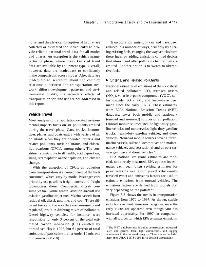
noise, and the physical disruption of habitat arecollected or estimated too infrequently to pro-vide reliable national trend data for all modesand phases. An exception is the vehicle manu-facturing phase, where many kinds of trenddata are available by equipment type. Overall,however, data are inadequate to confidentlymake comparisons across modes. Also, data areinadequate to generalize about the complexrelationship between the transportation net-work, diffuse development patterns, and envi-ronmental quality; the secondary effects oftransportation for land use are not addressed inthis report.
Vehicle TravelMost analyses of transportation-related environ-mental impacts focus on air pollutants emittedduring the travel phase. Cars, trucks, locomo-tives, planes, and boats emit a wide variety of airpollutants when they are operated: criteria andrelated pollutants, toxic pollutants, and chloro-fluorocarbons (CFCs), among others. The con-stituents contribute to ill health, acid deposition,smog, stratospheric ozone depletion, and climatechange.
With the exception of CFCs, air pollutionfrom transportation is a consequence of the fuelsconsumed, which vary by mode. Passenger carsprimarily use gasoline; freight trucks and freightlocomotives, diesel. Commercial aircraft con-sume jet fuel, while general aviation aircraft useaviation gasoline or jet fuel. Marine vessels burnresidual oil, diesel, gasoline, and coal. These dif-ferent fuels and the way they are consumed (andregulated) result in differing mixes of pollutants.Diesel highway vehicles, for instance, wereresponsible for only 3 percent of the total esti-mated carbon monoxide (CO) emitted byonroad vehicles in 1997, but 61 percent of totalemissions of particulate matter under 10 micronsin diameter (PM-10).
Transportation emissions can and have beenreduced in a number of ways, primarily by alter-ing existing fuels, changing the way vehicles burnthese fuels, or adding emissions control devicesthat absorb and alter pollutants before they areemitted. Another option is to switch to alterna-tive fuels.
� Criteria and Related PollutantsNational estimates of emissions of the six criteriaand related pollutants—CO, nitrogen oxides(NOX), volatile organic compounds (VOC), sul-fur dioxide (SO2), PM, and lead—have beenmade since the early 1970s. These estimates,from EPA’s National Emission Trends (NET)database, cover both mobile and stationary(onroad and nonroad) sources of air pollution.Onroad mobile sources include light-duty gaso-line vehicles and motorcycles, light-duty gasolinetrucks, heavy-duty gasoline vehicles, and dieselvehicles. Nonroad mobile sources cover aircraft,marine vessels, railroad locomotives and mainte-nance vehicles, and recreational and airport ser-vice gasoline and diesel vehicles.3
EPA national emissions estimates are mod-eled, not directly measured. EPA updates its esti-mates each year, often revising estimates forprior years as well. County-level vehicle-milestraveled (vmt) and emissions factors are used toestimate emissions from onroad vehicles. Theemissions factors are derived from models thatvary depending on the pollutant.
Figure 5-8 shows the trends in transportationemissions from 1970 to 1997. As shown, sizablereductions in most emissions categories since theearly 1980s are apparent even though vmt hasincreased appreciably. For 1997, in comparisonwith all sources for which EPA estimates emissions,
Chapter 5 Transportation, Energy, and the Environment � 117
3 The NET database also includes construction, industrial,lawn and garden, farm, light commercial, and loggingequipment in the nonroad category. These are not includedhere. (See USDOT BTS 1996 for a detailed discussion.)

118 � Transportation Statistics Annual Report 1999
1970 1973 1976 1979 1982 1985 1988 1991 1994 1997 0.00
0.20
0.40
0.60
0.80
1.00
1.20
1.40Carbon monoxide (CO) Nitrogen oxides (NOx)
Volatile organic compounds (VOC)
Particulate matter 2.5 microns in diameter or smaller (PM-2.5)
Ammonia
Lead
Particulate matter 10 microns in diameter or smaller (PM-10)
1970 1973 1976 1979 1982 1985 1988 1991 1994 1997 0.00
0.20
0.40
0.60
0.80
1.00
1.20
1.40
1970 1973 1976 1979 1982 1985 1988 1991 1994 1997 0.00
0.20
0.40
0.60
0.80
1.00
1.20
1.40
1970 1973 1976 1979 1982 1985 1988 1991 1994 1997 0.00
0.20
0.40
0.60
0.80
1.00
1.20
1.40
1970 1973 1976 1979 1982 1985 1988 1991 1994 1997 0.00
0.20
0.40
0.60
0.80
1.00
1.20
1.40
1970 1973 1976 1979 1982 1985 1988 1991 1994 1997 0.00
0.20
0.40
0.60
0.80
1.00
1.20
1.40
1970 1973 1976 1979 1982 1985 1988 1991 1994 1997 0.00
0.20
0.40
0.60
0.80
1.00
1.20
1.40
NOTE: In estimating criteria and related pollutant emissions for 1997,the Environmental Protection Agency (EPA) made adjustments to prioryears. For onroad mobile sources, EPA revised 1996 data. For nonroadmobile sources, EPA revised some estimates back to 1970. The figurereflects those changes and supercedes the similar figure 4-8 in Trans-portation Statistics Annual Report 1998.
SOURCE: U.S. Environmental Protection Agency, Office of Air andRadiation, Air Quality Planning and Standards, National Air PollutionEmission Trends, 1900–1997, available on the EPA website at www.epa.gov/ttn/chief/trends97/emtrnd.html.
1970 = 1.0; 1990 = 1.0 for PM-2.5 and ammonia
Figure 5-8National Transportation Emissions Trends Index: 1970–97

mobile sources contributed 62 percent (53,842,000short tons) of all CO, 36 percent (8,573,000 shorttons) of NOX, 32 percent (6,138,000 short tons) ofVOC, and 13 percent (522 tons) of lead. Mobilesource lead emissions have declined significantlysince 1970 when they were 82 percent of all leademissions. Today, vehicle-use lead emissions comeprimarily from general aviation, nonroad engines,marine vessels, and motor racing vehicles fuels (63Federal Register 49240).
While mobile sources are only responsible for1 percent (414,000 short tons) of PM-10 emis-sions, the contribution rises to 4 percent(324,000 short tons) for the smaller size PM-2.5emissions (particulate matter of 2.5 microns or
smaller). EPA has added a new pollutant for1997—ammonia—with data estimated back to1990. Mobile sources provided 8 percent (243tons) of total ammonia emissions in 1997.Onroad gasoline vehicles generated 98 percent ofmobile source emissions from ammonia; the bal-ance came from highway diesel vehicles, rail-roads, and marine vessels. Gaseous ammoniareacts in the air with SO2 and NOX, resulting inammonium sulfate and nitrate particles that arefound in PM-2.5. As figure 5-8 shows, estimatedannual mobile source ammonia emissions havebeen erratic but have risen sharply since 1990.
Modal shares of the 1997 emissions of fivepollutants are shown in figure 5-9. When com-
Chapter 5 Transportation, Energy, and the Environment � 119
CO
NOX
VOC
PM-10
Lead
0 10 20 30 40 50Percent
60 70 80 90 100
Onroad gasoline Onroad diesel Aircraft Commercial marine Railroad Other nonroad
KEY: CO = carbon monoxide; NOX = nitrogen oxides; PM-10 = particulate matter 10 microns in diameter or smaller; VOC = volatile organic compounds.
NOTES: Other nonroad includes recreational vehicles, recreational marine vessels, airport service vehicles, and railroad maintenance equipment. Does not include farm, construction, industrial, logging, light commercial, and lawn and garden equipment.
SOURCE: U.S. Environmental Protection Agency, Office of Air and Radiation, Air Quality Planning and Standards, National Air Pollution Emission Trends, 1990–1997, available on the EPA website at www.epa/ttn/chief/trends97/emtrnd.html.
Figure 5-9Modal Shares of Key Criteria Pollutants from Transportation Sources: 1997
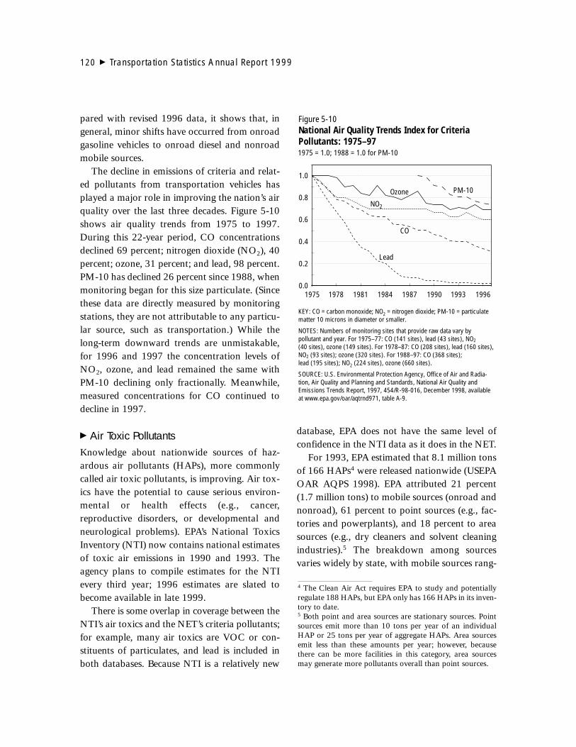
pared with revised 1996 data, it shows that, ingeneral, minor shifts have occurred from onroadgasoline vehicles to onroad diesel and nonroadmobile sources.
The decline in emissions of criteria and relat-ed pollutants from transportation vehicles hasplayed a major role in improving the nation’s airquality over the last three decades. Figure 5-10shows air quality trends from 1975 to 1997.During this 22-year period, CO concentrationsdeclined 69 percent; nitrogen dioxide (NO2), 40percent; ozone, 31 percent; and lead, 98 percent.PM-10 has declined 26 percent since 1988, whenmonitoring began for this size particulate. (Sincethese data are directly measured by monitoringstations, they are not attributable to any particu-lar source, such as transportation.) While thelong-term downward trends are unmistakable,for 1996 and 1997 the concentration levels ofNO2, ozone, and lead remained the same withPM-10 declining only fractionally. Meanwhile,measured concentrations for CO continued todecline in 1997.
� Air Toxic PollutantsKnowledge about nationwide sources of haz-ardous air pollutants (HAPs), more commonlycalled air toxic pollutants, is improving. Air tox-ics have the potential to cause serious environ-mental or health effects (e.g., cancer,reproductive disorders, or developmental andneurological problems). EPA’s National ToxicsInventory (NTI) now contains national estimatesof toxic air emissions in 1990 and 1993. Theagency plans to compile estimates for the NTIevery third year; 1996 estimates are slated tobecome available in late 1999.
There is some overlap in coverage between theNTI’s air toxics and the NET’s criteria pollutants;for example, many air toxics are VOC or con-stituents of particulates, and lead is included inboth databases. Because NTI is a relatively new
database, EPA does not have the same level ofconfidence in the NTI data as it does in the NET.
For 1993, EPA estimated that 8.1 million tonsof 166 HAPs4 were released nationwide (USEPAOAR AQPS 1998). EPA attributed 21 percent(1.7 million tons) to mobile sources (onroad andnonroad), 61 percent to point sources (e.g., fac-tories and powerplants), and 18 percent to areasources (e.g., dry cleaners and solvent cleaningindustries).5 The breakdown among sourcesvaries widely by state, with mobile sources rang-
120 � Transportation Statistics Annual Report 1999
0.0
0.2
0.4
0.6
0.8
1.0
CO
Lead
NO2
Ozone PM-10
1975 1978 1981 1984 1987 1990 1993 1996
KEY: CO = carbon monoxide; NO2 = nitrogen dioxide; PM-10 = particulatematter 10 microns in diameter or smaller.
NOTES: Numbers of monitoring sites that provide raw data vary by pollutant and year. For 1975–77: CO (141 sites), lead (43 sites), NO2 (40 sites), ozone (149 sites). For 1978–87: CO (208 sites), lead (160 sites),NO2 (93 sites); ozone (320 sites). For 1988–97: CO (368 sites); lead (195 sites); NO2 (224 sites), ozone (660 sites).
SOURCE: U.S. Environmental Protection Agency, Office of Air and Radia-tion, Air Quality and Planning and Standards, National Air Quality andEmissions Trends Report, 1997, 454/R-98-016, December 1998, available at www.epa.gov/oar/aqtrnd971, table A-9.
1975 = 1.0; 1988 = 1.0 for PM-10
Figure 5-10National Air Quality Trends Index for CriteriaPollutants: 1975–97
4 The Clean Air Act requires EPA to study and potentiallyregulate 188 HAPs, but EPA only has 166 HAPs in its inven-tory to date.5 Both point and area sources are stationary sources. Pointsources emit more than 10 tons per year of an individualHAP or 25 tons per year of aggregate HAPs. Area sourcesemit less than these amounts per year; however, becausethere can be more facilities in this category, area sourcesmay generate more pollutants overall than point sources.

ing from 55 percent in Hawaii to 10 percent inAlabama. EPA estimated that in 1993 HAPsreleased by onroad gasoline vehicles (1.3 milliontons) were 16 percent below its 1990 estimatedue to use of reformulated fuels required toreduce urban ozone. These data also show thatonroad gasoline vehicles emit 76 percent of allmobile source HAPs.6
In the 1990s, EPA regulated air toxics throughmaximum achievable control technology stan-dards, directed primarily at stationary pointsources. Because of a CAA mandate, EPA pub-lished a draft Integrated Urban Air ToxicsStrategy in September 1998 (63 Federal Register49240). The strategy provisionally identifies 33air toxics as presenting the greatest health risksin urban areas. Mobile sources emitted almost40 percent of these pollutants in the base year,1990 (see table 5-3).
EPA expects to publish a final IntegratedUrban Toxics Strategy by June 1999 and is con-
Chapter 5 Transportation, Energy, and the Environment � 121
6 In this and other sections where data other than the NETare used, it has not been possible to eliminate subcategoriesof nonroad mobile sources mentioned in the criteria pollu-tant section.
Table 5-3Mobile Source Urban Hazardous Air Pollutants: 1990 Base Year(Estimated tons per year)
Onroad % of Nonroad % of Nonroad % ofChemical vehicles totala aircraft totala other totala
1,3 butadiene 36,920 47.7 854 1.1 16,628 21.5Acetaldehyde 28,163 27.5 2,090 2.0 6,394 6.2Acrolein 8,152 11.6 989 1.4 5,376 7.7Arsenic and compounds 2 0.1 — —Benzene 208,740 47.6 1,106 0.3 89,998 20.5Chromium and compounds 28 2 — 17 1.2Dioxins/furans 9.5 x 10⁻⁵ 1.6 — —Formaldehyde 97,506 35.6 6,791 2.5 26,864 9.8Lead and compounds 1,690 35.8 384 8.1 197 4.2Manganese and compounds 22 0.7 — 20 0.6Nickel and compounds 16 0.9 — 9 0.5Polycyclic organic matter as 16-PAH 76 0.3 5 <0.1 47 0.2
Subtotal 381,314 12,219 145,551Polycyclic organic matter as 7-PAH 34 1.7 <0.1 <0.1 24 1.2Polycyclic organic matter as EOM 56,157 13.9 — —Styrene 17,200 38.8 194 0.4 4,657 10.5
Total 454,705 12,412 15,232a Percentage of total emissions, all sources, both urban and rural.
KEY: EOM = extractable organic matter; PAH = polycyclic aromatic hydrocarbon; — = less than 0.01 or no estimate made.
NOTES: Chemicals in italics are those for which the Environmental Protection Agency estimated base-year emissions data; they are not included on the currentlist of 33 draft urban hazardous air pollutants (HAPs).
SOURCES:For data: U.S. Environmental Protection Agency, Office of Air and Radiation, Air Quality Strategies and Standards Division and Emissions, Monitoring, andAnalysis Division, 1990 Emissions Inventory of Forty Section 112(k) Pollutants, Interim Final Report, available at www.epa.gov/ttn/uatw/112k/112kfac.html,January 1998.
List of 33 draft urban HAPs:U.S. Environmental Protection Agency, Office of Air and Radiation, Air Quality Planning and Standards, National Air Quality and Emissions Trends Report,1997, 454/R-98-016, December 1998, available at www.epa.gov/oar/aqtrnd97/, table 5-4.

currently updating a 1993 study on the cancereffects of several mobile source pollutants.Subsequently, EPA plans to promulgate nationalregulations to control HAP emissions frommotor vehicles and fuels, as well as from pointand area sources.
� Stratospheric Ozone DepletionCFCs and other chemicals deplete the stratos-pheric ozone layer that protects the earth fromharmful ultraviolet rays. Before production washalted at the end of 1995, CFC-12 was widelyused as the refrigerant for mobile air conditioning(MAC) systems in cars, trucks, and other vehi-cles. In the late 1980s, MAC systems accountedfor 37 percent of total CFC-12 use (Oldenburgand Hirschhorn 1991). The last new MAC unitswith CFC-12 were shipped in 1994. These unitsare expected to have a lifetime of 12 years, thusemissions—while declining—are expected to con-tinue to 2006. Emissions of CFC-12 from pre-1995 units occur from leaks during use, whilebeing serviced, and at disposal. Servicing isexpected to consume 84 percent of the stocks ofCFC-12 available in 1998 (USEPA OAR SPD1998). An estimated 66 million MAC units werestill in operation in 1998 in the United States.
The primary replacement chemical for MACunits has been HFC-134a, although EPA nowlists nine other acceptable alternates. Depart-ment of Energy preliminary estimates of 1997emissions from all sources, including transporta-tion, list 24,000 metric tons of CFC-12 and18,000 metric tons of HFC-134a. During theperiod 1990 to 1996, CFC-12 emissions declinedby 68 percent, while HFC-134a emissions,which are not ozone-depleting, rose 13 percent(USDOE 1998e).
� Aircraft Cruise Emissions Only criteria pollutant emissions during aircraftlanding and takeoff (LTO) are included in EPA’s
NET data on aircraft emissions. Aircraft engines,however, also emit pollutants, such as CO2,NOX, and water vapor while cruising. The quan-tity of aircraft pollutants emitted is a function ofthe type of aircraft and engine, modes of opera-tion—taxi/idle-out, takeoff, climb-out, cruise,approach, and taxi/idle-in—and how longengines are operated in each mode.
Cruise-level pollutants are a concern becauseof their potential impact on global atmosphericproblems, such as stratospheric ozone depletionand climate change. However, the extent of theseemissions and their impacts are not well known.A Special Report on Aviation and the GlobalAtmosphere by the Intergovernmental Panel onClimate Change (IPCC 1999) will be used by theInternational Civil Aviation Organization(ICAO) to consider potential reduction solutionsin three categories: changes in technology, oper-ational measures, and market-based options.
A Federal Aviation Administration (FAA)report suggests that air traffic control opera-tional changes that reduce flight restrictions andresult in improved aircraft fuel efficiencies couldlower NOX emissions by 10 percent, CO by 13percent, and hydrocarbons by 18 percent. Over90 percent of these reductions would occur dur-ing flight phases above 3,000 feet (USDOT FAA1998a). Between 1975 and 1995, U.S. airlinesimproved fuel efficiency by about 44 percentthrough technical and operational changes(USDOT BTS 1998a).
� Pipeline EmissionsThere are over 200,000 miles of petroleum and1.3 million miles of natural gas pipeline in theUnited States (USDOT BTS 1998a, table 1-8).EPA’s AIRS Facility Subsystem (AFS) providesinsight into the type and magnitude of pipelineemissions. However, because of the physical dif-ferences between pipelines and other modes andthe ways in which AFS data are collected, the
122 � Transportation Statistics Annual Report 1999

data are difficult to use. Comparisons cannot bemade using AFS facility-based and NET mobilesource data.
According to the AFS, pipelines emit all of thecriteria and related pollutants, as well as toxicpollutants as do other modes. Petroleum pipelinedata systems (SIC 46) are more likely to emitmore SO2 and VOC than do natural gas pipelinesystems (SIC 49). The latter emit more CO, PM-10, and NO2. Pipelines also emit a variety ofHAPs. For a natural gas distribution system (SIC4924), one state estimated emissions at the coun-ty level of 77 pounds per year of total HAPs. Inaddition, the record shows emissions of nickel,phenol, toluene, xylenes, formaldehyde, mer-cury, manganese, and cadmium. The latter threeare listed as constituents of total suspended par-ticulate emissions (USEPA OAR AQPS 1999a).
Other Vehicle Travel ImpactsWhile far less quantitative information is avail-able, it is known that transportation vehiclesduring use impact the environment in manyother ways besides emitting air pollutants.Common to all modes is the problem of acci-dents and leaks that result in spills of hazardousmaterials, including crude oil and petroleumproducts. Noise pollution affects people who liveor work along highways, railways, and near air-ports. Other impacts include fugitive dust emis-sions from roads, oil and coolant releases fromlocomotives, roadkill, habitat disruption, intro-duction of nonnative species, and dumping ofsolid waste and sewage from marine vessels.
� Noise The transportation system creates pervasivenoise, degrading the quality of life to thoseexposed. Primary sources are aircraft LTOs andtraffic moving along highways and railways.Although there are no national trend data onnoise, national standards have been developed
by FAA for aircraft and by EPA for medium andheavy highway trucks, motorcycles, locomotives,and railcars.
Noise is measured in decibels (dB) thatincrease as amplitude doubles or in the A-weighted scale (dBA) that emphasizes sound fre-quencies people hear best. At 65 dBA noisebecomes annoying; 128 dBA is the pain thresh-old (USDOT BTS 1996, 151). Highway trucksmanufactured after January 1988 are subject toa maximum rating of 80 dBA. The standard formotorcycles varies from 70 to 82 dBA dependingon the model year (1983 to 1989) and type andwhether or not the purchaser is the federal gov-ernment (49 CFR Part 205). Noise standards forlocomotives manufactured after December 1979range from 70 to 90 dBA depending on whetherthe locomotives are moving or stationary.Railcars moving more than 45 miles per hourhave a limit of 93 dBA. Various standards alsoapply to railroad switching equipment used inrailyards (49 CFR Part 210).
Aircraft LTO noise has come under the mostrecent scrutiny. Stage 3 noise-certified aircraft arebeing phased in according to regulations promul-gated under the Aircraft Noise and Capacity Actof 1990. Stage 3 aircraft noise levels range from95 to 105 dBA and differ depending on aircraftweight and LTO operations. By the end ofDecember 1999, all aircraft weighing over 75,000pounds using U.S. airports must be Stage 3 certi-fied. In August 1998, FAA reported to Congressthat 260 domestic and foreign operators hadreached a combined fleet mix of 79.8 percentStage 3 aircraft by the end of December 1997.This was an increase of 4.3 percent over the Stage3 fleet mix a year earlier (USDOT FAA 1998b).
� Spills of Oils and Hazardous MaterialsMode operators are required by law to reportspills of hazardous materials, such as oxidizers,combustible liquids and gases, and corrosive
Chapter 5 Transportation, Energy, and the Environment � 123

material. Three data sources provide informa-tion on the extent and cost of spills. The U.S.Department of Transportation’s (DOT’s)Hazardous Materials Information System(HMIS) records reported hazardous materialsincidents by four modes: highway, rail, air, andwater.7 DOT’s Integrated Pipeline InformationSystem in the Office of Pipeline Safety aggregatesincident data reported by hazardous liquidpipeline operators and natural gas pipeline dis-tribution and transmission operators. These twodatabases contain the numbers, costs, and caus-es of incidents, the number of injuries and deathscaused by the incidents, and the type and volumeof commodities spilled.
The U.S. Coast Guard’s Modified MarineSafety Information System contains data on oilpollution incidents occurring in U.S. waters. Datareleased in 1999 show that in 1993 through 1998there were approximately 9,000 spills on averageeach year. The yearly average over this time peri-od for volume of oil spilled is approximately 2million gallons. It should be noted that for 1997and 1998 the volume of oil spilled fell below 1million gallons (USDOT USCG 1999). While,historically, the amount spilled each year can varygreatly, these data show a continuation of anoverall decline since the early 1970s (see USDOTBTS 1996).
HMIS data show that four modes (highway,air, water, and rail) together averaged 14,385hazardous materials incidents per year between1993 and 1997. Highway vehicles were thesource of 86 percent of these incidents. This doesnot necessarily mean that highway vehicles aremore prone to hazardous materials accidents,since the data are not normalized by, for in-stance, vmt, number of trips, or commodity
flows by mode. Two classes of hazardous mate-rials—flammable/combustible liquids and corro-sive materials—are involved in almost 80 percentof each mode’s incidents, a likely consequence ofthese substances being among the most widelyshipped in the United States. Combustible liquidsinclude gasoline, petroleum products, and sol-vents; and corrosive materials include cleanersand acids (USDOT OHMS 1998).
Hazardous liquid pipelines incurred an aver-age of 200 incidents per year between 1988 and1997 resulting in an average of 2 deaths, 16injuries, $34 million in damages, and a net lossof 85,000 barrels of liquid per year. Outsidedamage and external corrosion were the prima-ry cause of hazardous liquid pipeline incidents in1997 (USDOT OPS 1998).
Natural gas transmission and distributionoperators reported a 1988 to 1997 average of 215incidents per year, resulting in 18 fatalities, 91injuries, and $32 million in property damage. In1997, the primary cause of natural gas pipelineincidents was damage from outside forces. Fortransmission pipelines alone, internal corrosionranked second. At the conclusion of a 1996 liquidpipeline accident investigation, the NationalTransportation Safety Board recommended in late1998 that the DOT Office of Pipeline Safety makeseveral changes to federal regulations to improvethe pipeline industry’s ability to prevent accidentalreleases caused by corrosion (USDOT OPS 1998).
Infrastructure Developmentand OperationAll transportation vehicles require supportinginfrastructure, such as highways and bridges, raillines and terminals, airports, and marine portsand marinas. In a sense, pipelines could be viewedas stationary vehicles or infrastructure throughwhich commodities pass. All modes require fuel-ing stations or equipment, and servicing andrepair facilities. Establishment (and enlargement)
124 � Transportation Statistics Annual Report 1999
7 HMIS water data are limited to nonbulk shipments on ves-sels, and cover all U.S. waters and U.S. carriers wherever theymay be at the time of the incident. Coverage does not includemajor incidents such as tanker spills, which are in the U.S.Coast Guards’ Modified Marine Safety Information System.

of these facilities and infrastructure takes land,disrupting the habitats of people and wildlife whowere prior users of the space, while their con-struction, maintenance, and operation generatesair and water pollutants, wastes, and noise.
Repairs to roads and railways create wastes,such as railroad ties and rails, concrete, and asphaltpavement. Oil, soot, grease, and chemicals run offroads, airports, railyards, and maintenance facili-ties with the potential to pollute surface waters orseep into and contaminate underground water.Vehicles themselves do not contribute much to par-ticulate emissions but fugitive dust from paved andunpaved roads generated 44 percent (14.8 milliontons) of all PM-10 and 30 percent (2.5 milliontons) of all PM-2.5 emissions in 1997 (USEPAOAR AQPS 1999b). The following sections high-light marine facilities and airports.
Marine FacilitiesThere are more than 1,900 major coastal sea-ports and Great Lakes terminals, nearly 3,200berths in the United States, and over 1,800 riverterminals are located in 21 states (USDOT BTSMARAD USCG 1999). During operation, shipsgenerate garbage, sewage, and bilge and ballastwaters. Bilge water consists of fuel, oil, onboardspills, and wash waters generated during dailyoperations, as well as solid wastes, such as rags,metal shavings, paint, glass, and cleaning agents.Ballast waters from tankers may contain cargoresidues, such as petroleum products. The inter-national Maritime Pollution Convention of1978, to which the United States is a signatory,covers discharges of these and other substancesfrom ships at sea. Raw sewage, for instance, canbe discharged 12 miles from land (USEPA OECA1997). If not dischargable at sea, ship wastes aresupposed to be unloaded while in ports. Portsthen become responsible for proper managementof the wastes. Port facilities that maintain andrepair marine vessels generate additional wastes.
Ports and navigation channels must be peri-odically dredged to maintain proper depth andfor enlargement. From 1993 to 1997, the U.S.Army Corps of Engineers dredged an average of273 million cubic yards of material per yearfrom navigation channels at an annual averagecost of $542 million (USACE 1998). Dredgedmaterials, if classified as hazardous or toxic, mayhave to be disposed of in confined facilitiesrather than used beneficially, such as for beachnourishment or fill for industrial or urban devel-opment.
� Airport Infrastructure OperationsAirports are an example of transportationinfrastructure where modes converge. Airplanesland and take off. Highway vehicles (automo-biles, trucks, and buses) deliver and pick upgoods and passengers. At some airports, transitrail and ferries may also transport passengers.Airport facilities operate, repair, and maintainaircraft and supporting vehicles. Airports alsosupply services to passengers and workers, suchas food, shopping, and restrooms. All theseactivities have the potential to impact publichealth and the environment within the airportand surrounding areas.
There were 566 civil, certificated airports8 inthe United States in 1997 (USDOT BTS 1998a,table 1-2). These airports differ greatly in size andhow they operate. In most cases, a local govern-ment owns the airport and leases the facilities toairlines, service businesses, and other operators.Chicago O’Hare International Airport, which isone of the largest in the world, handled approxi-mately 38 million enplaned passengers in 1998(USDOT BTS OAI 1999). It has 162 aircraftgates in 4 terminal buildings and in 1994 hadmore than 380,000 aircraft departures (USDOT
Chapter 5 Transportation, Energy, and the Environment � 125
8 Certificated airports serve air carrier operations with air-craft seating more than 30 passengers.

FAA n.d., table 4-8). Given the wide variety ofactivities and multiple operators, data on airportimpacts must be aggregated or disaggregatedfrom various sources. Still, a complete quantita-tive picture of environmental impacts does notemerge.
EPA’s criteria pollutant data include airportservice equipment in its nonroad mobile catego-ry, but there are no national data on emissions ofonroad mobile sources specific to airports. TheNET contains aircraft LTO data (see table 5-4).Aircraft emissions estimates for 1997 range from4 percent of total NOX nonroad 1997 emissionsto 100 percent of lead emissions. The percent-ages increase somewhat when service equipmentemissions are added, with NOX rising to 6 per-cent, largely due to the use of diesel equipment.Worldwide LTO standards for NOX, CO, andunburned hydrocarbons (such as VOC) are setby ICAO.9
EPA’s inventory of 33 urban air toxics attrib-utes emissions of more than 12,000 tons of these
pollutants to aircraft LTO operations (see table5-3 above) (USEPA OAR AQSSD/EMAD 1998).This represents 8 percent of the estimated totalnonroad toxic air emissions and includes 1,3-butadiene, acetaldehyde, acrolein, benzene,formaldehyde, and lead. The use by general avi-ation aircraft of aviation gasoline results in leademissions.
EPA’s Biennial Reporting System on Haz-ardous Waste has data on Airports, Flying Fields,and Services (SIC 4581) for the years 1989,1991, 1993, and 1995. EPA, however, does notaggregate and publish the data by SIC. Airportreporting appears to be inconsistent from oneyear to the next, which most likely results fromreporting rules; a facility may have to report oneyear but not the next depending on the quantityof waste generated and changes in the way afacility manages these wastes. For instance,Buffalo Airport, New York, only reported in1995. In Virginia, Dulles International Airportreported in 1991, 1993, and 1995; NationalAirport, only in 1995. Dulles reported that itsshops and warehouse building activities generat-ed an average of 53 tons of hazardous waste per
126 � Transportation Statistics Annual Report 1999
Table 5-4Aircraft-Related Criteria Pollutants Emitted at Airports: 1997(Short tons)
Source CO NOX VOC SO2 PM-10 Lead
Aircraft, landing and takeoff 1,012,026 177,521 186,923 11,914 40,924 503% of total (nonroad mobile sources) 6.0 3.9 7.7 1.1 8.8 100.0
Airport service equipmentGasoline 140,657 3,192 6,436 0 36 0Diesel 42,995 93,242 10,757 0 11,343 0
Total aircraft and service equipment 1,195,678 273,955 204,116 11,914 52,303 503% of total (nonroad mobile sources) 7.1 6.0 8.4 1.1 11.2 100.0
KEY: CO = carbon monoxide; NOX = nitrogen oxides; PM-10 = particulate matter 10 microns in diameter or smaller; SO2 = sulfur dioxide; VOC = volatile organic compounds.
SOURCE: U.S. Environmental Protection Agency, Office of Air and Radiation, Air Quality Strategies and Standards, National Air Pollutant Emission Trends,1900–1997, forthcoming on the EPA website, 1999.
9 Countries belonging to ICAO can accept the standards orpetition ICAO to be exempted. In April 1997, the UnitedStates adopted ICAO NOX and CO emissions standards forcommercial aircraft engines.

year. Among the listed items were degreasingparts cleaner, roof caulking, flammable and cor-rosive liquids, unused pesticides, mixed freons,and toluene. Some of the largest quantities andvarieties of hazardous wastes are reported sepa-rately by airline company maintenance facilities.United Airlines’ maintenance operations facilityat San Francisco International Airport reportedin all years except 1989. The facility generatedan average of 2,285 tons of hazardous waste peryear (USEPA OSW 1999).10
Hazardous materials spills occur primarilyduring aircraft cargo loading and unloading oper-ations and from leaking storage tanks, mainly ofpetroleum products. According to HMIS data,the air mode averaged 864 spills per year, or 6percent of all mode spills from 1993 to 1997(USDOT OHMS 1998). Flammable/combustibleliquids and corrosive materials constitute 78 per-cent of annual spills. Airports store aircraft fuel inaboveground and underground tanks that havethe potential to leak. Federal regulations do notcover aboveground tanks of petroleum productsunless they are part of a pipeline facility, and EPAhas deferred action on underground tanks at air-ports. Thus, the EPA Corrective Action Measuresdatabase on underground tanks does not includeairport tanks. Some states, such as Florida andVirginia, are moving toward addressing the issueof the leaks themselves. Virginia is working on acase-by-case basis with airport developmentplans to assure that storage technology upgradesand leak detection systems are included. TheAerospace Industries Association and theAmerican Petroleum Institute are conducting astudy on leak detection technologies for airportfuel storage systems.
An important airport environmental issue isrunoff into surface waters and soil of deicing
chemicals used during winter months. A summa-ry of deicing and anti-icing of aircraft and air-port runways was presented in TSAR98. Someregulatory measures are underway that couldprovide more information and may alter airportpollutant-generating activities. In early 1997,EPA’s Toxics Release Inventory (TRI) office re-ceived a petition from environmental groups toadd SIC 45 (Transportation by Air) to its annualreporting system. A decision will not be madeuntil late 1999 or early 2000.11 If the sector isadded to the TRI, airports that meet thresholdlevels of emissions will have to report on certaintoxic releases to air, water, and land.
In another effort, EPA’s Office of Water isconducting a preliminary study on airportdeicing that is scheduled for completion in late1999 (63 Federal Register 29203). The studyresults could prompt development of a guid-ance document or regulations leading to efflu-ent guidelines for airports.
Vehicle and Parts ManufacturingFactories that manufacture transportation vehi-cles and parts generate air and water pollutantsand solid wastes, some of which are classified ashazardous.12 Many of these facilities are requiredto report annually to the TRI on their releasesand transfers of toxic chemicals. This informa-tion will help determine the environmental im-pacts of vehicle and parts manufacturing.However, differences between TRI data and theNET criteria and related pollutant data that EPAestimates for mobile sources make comparisons
Chapter 5 Transportation, Energy, and the Environment � 127
10 The average was calculated using 1989, 1991, 1993, and1995 data from U.S. Environmental Protection Agency(USEPA OSW 1993–97).
11 An EPA working group must first report on the currentTRI motor vehicle exemption. 12 This section does not cover pipeline manufacturing andonly reviews the final manufacturing and assembly stagesrelated to highway, air, marine, and rail vehicles and parts.A more comprehensive review, such as during a life-cycleassessment, would also consider environmental impactsfrom primary stages, such as raw material extraction andrefining.

with other phases of the transportation systemdifficult.
TRI data are estimated by facilities, but thefacilities do not have to report emissions below athreshold.13 The list of TRI chemicals haschanged from year to year. Some have beenremoved because they were determined not tomeet the criteria for listing; others have beenadded. The list started in 1987 (the first report-ing year) with 308 chemicals; in 1995, it con-tained more than 600 chemicals and 28 chemicalcategories. The set of criteria pollutants hasremained constant since the 1970s. Of the crite-ria pollutants, CO, NOX, and SO2 are not on theTRI list; lead is, however. In addition, some ofthe chemicals on the TRI qualify as VOC or con-stituents of particulates (PM-10 or PM-2.5).Chemicals in EPA’s air toxics inventory (the NTI)are a subset of those in the TRI.
Analysis of the environmental impact of trans-portation equipment manufacturing is also compli-cated by the sizable international trade in thisindustry. Thus, the environmental impacts frommanufacturing in the United States are not propor-tional to the numbers of vehicles American’s use.For instance, over 12 million passenger cars, trucks,and buses were produced in the United States in1994 (AAMA 1995). Many of the parts for thesevehicles may be imported. Furthermore, while justover 1 million cars, trucks, and buses produced inthe United States were exported in 1994, importstotaled almost 5 million vehicles. Data on the valueof other modal vehicle trade show U.S. exportsexceed imports, especially for civilian aircraft. Oneexception may be motorcycles and parts; 1997 datalist only imports (USDOC 1998).
� Toxic Pollutants14
Facilities in the transportation equipment manu-facturing (TEM—SIC 37) sector report to EPA’sTRI annually on environmental releases of toxicair and water pollutants and hazardous wastes.They also report on the transfers of these chemi-cals offsite of their facilities (for recycling, energyrecovery, treatment, and disposal) and to pub-licly owned treatment works.15
Among the manufacturing sectors that report-ed 1996 data to the TRI, TEM is ranked fourthin total onsite releases and sixth in total transfersoffsite (USEPA OPPT 1999). Table 5-5 comparesthe sector’s releases and transfers by mode. Itshows that highway vehicle and parts manufac-turers were responsible for 65 percent of the sec-tor’s releases and 77 percent of the transfers in1996. For all modes, air emissions were the mostsignificant in terms of total pounds releasedonsite. Just 15 chemicals contributed 92 percentof all these releases. They include xylene, styrene,glycol ethers, toluene, methyl ethyl ketone, man-ganese, and others.
EPA has compared year-to-year SIC 37 TRIdata, based on a core set of chemicals that havebeen consistently reported. Between 1988 and1996, subsectors (by 4-digit SIC) have reducedonsite releases, ranging from 34 percent formotor vehicle and car bodies (SIC 3711) to 96percent for aircraft engines (SIC 3724). Most ofthe reductions are due to lower air emissions. Anexception is SIC 3751 (motorcycles, bicycles,
128 � Transportation Statistics Annual Report 1999
13 Manufacturing facilities in SICs 20–39 report if they have10 or more full-time employees and release/transfer frommanufacturing or processing more than 25,000 pounds of alisted chemical or more than 10,000 pounds from “other-wise use.” Methods of estimation used by facilities can vary.
14 The basis for this discussion is facilities that report to theTRI under SIC 37 (transportation equipment industry).However, many vehicle parts are manufactured by facilitiesthat report under other SICs. They include tires (SIC 30),automotive glass (SIC 32), batteries and lighting systems(SIC 36), portions of engines (SIC 35), and automotive seats(SIC 25). In addition, the stamping process is represented infabricated metals (SIC 34). In most of these categories, vehi-cle parts data are comingled with data on other products. 15 Facilities must also report on the amount of and how theymanage chemicals onsite. These data are not included in thisdiscussion.

Chapter 5 Transportation, Energy, and the Environm
ent�
129
Table 5-5Toxic Release Inventory Data for Transportation Equipment Manufacturing: 1996(In pounds, except as noted)
Surface Under- TotalAir water ground Land onsite For For waste Total
Sector by mode SIC emissions discharges injection releases releases disposal a management b offsite Totals
Motor vehicle and car bodies 3711 40,561,496 10,428 0 15,310 40,587,234 1,517,251 46,128,216 47,645,467 88,232,701Truck and bus bodies 3713 4,719,018 3,257 0 47,986 4,770,261 133,698 4,308,171 4,441,869 9,212,130Motor vehicle parts
and accessories 3714 15,634,030 83,564 0 363,251 16,080,845 4,348,414 103,728,587 108,077,001 124,157,846Truck trailers 3715 1,705,764 265 0 115,727 1,821,756 16,370 996,221 1,012,591 2,834,347Motorcycles, bicycles, and parts 3751 721,200 0 0 0 721,200 9,050 679,411 688,461 1,409,661
Highway vehicles total 63,341,508 97,514 0 542,274 63,981,296 6,024,783 155,840,606 161,865,389 225,846,685
Aircraft 3721 4,247,896 16,719 0 15,866 4,280,481 62,547 2,283,762 2,346,309 6,626,790Aircraft engines and engine parts 3724 484,200 86,909 0 73,773 644,882 430,432 11,984,305 12,414,737 13,059,619Aircraft parts and equipment, nec 3728 2,396,026 324 0 15,949 2,412,299 120,680 2,504,350 2,625,030 5,037,329
Aircraft total 7,128,122 103,952 0 105,588 7,337,662 613,659 16,772,417 17,386,076 24,723,738
Ship building and repairing 3731 2,707,317 19,752 0 23,922 2,750,991 191,201 7,760,908 7,952,109 10,703,100Boat building and repairing 3732 11,274,153 0 0 27,134 11,301,287 11,007 469,057 480,064 11,781,351
Marine vessels total 13,981,470 19,752 0 51,056 14,052,278 202,208 8,229,965 8,432,173 22,484,451
Railroad equipment 3743 1,328,150 1 0 1 1,328,152 210,868 1,983,439 2,194,307 3,522,459Railroad total 1,328,150 1 0 1 1,328,152 210,868 1,983,439 2,194,307 3,522,459
Miscellaneousc 12,323,358 2,901 0 5,501 12,331,760 578,421 18,724,061 19,302,482 31,634,242
Total (pounds) 98,102,608 224,120 0 704,420 99,031,148 7,629,939 201,550,488 209,180,427 308,211,575TOTAL (tons) 49,051 112 0 352 49,516 3,815 100,775 104,590 154,106
a Disposal is an environmental release that occurs offsite.b Waste management categories include recycling, energy recovery, treatment, and publicly owned treatment works.c Data for facilities that reported more than one Standard Industrial Classification (SIC) 37.
NOTES: This table does not include data for all facilities that report under SIC 37. Space vehicles, guided missiles, and parts (SIC 3761, 3764, and 3769), travel trailers and campers (SIC 3792), tanks and tankcomponents (SIC 3795), and transportation equipment not elsewhere classified (nec) (SIC 3799) have been excluded.
SOURCE: U.S. Environmental Protection Agency, Office of Prevention, Pesticides, and Toxic Substances, 1996 Public Data Release: Ten Years of Right-To-Know, available atwww.epa.gov/opptintr/tri/pdr96/2drhome.htm, 1999.
Onsite releases Transfers offsite

and parts), which increased total onsite releasesby 125 percent between 1988 and 1996.
� Criteria and Related Air PollutantsCurrent data sources do not provide data compa-rable to that of mobile sources on the emissions ofcriteria and related pollutants from TEM. AIRSAFS contains data for key SIC 37 categories, butnot necessarily for all facilities nationwide (seeabove). For the NET, EPA makes national emis-sions estimates for stationary sources but does notnecessarily align them with SICs.
The NET does not contain data for all sta-tionary source categories across all pollutantcategories. For the transportation equipmentindustry, EPA estimates CO, NOX, and VOCemissions. For 1997 and prior years, CO andNOX emissions estimates are zero, whichmeans they are less than 1 ton. Using AIRSdata, however, EPA’s Office of Enforcementand Compliance Assurance estimated that justthree TEM sectors—motor vehicles and bod-ies, motor vehicle parts and accessories, andshipbuilding and repair—emit over 15,000tons of CO and 28,000 tons of NO2 per year(USEPA OECA 1998). Under the NET’s sol-vent utilization category, EPA shows VOCemissions for surface coating of autos and lighttrucks, large ships, aircraft, and railroad vehi-cles. EPA also estimates VOC emissions fromrubber tire manufacturing. The combinedVOC emissions for these source categories, aswell as TEM, total 162 tons for 1997; surfacecoating of autos and light trucks are 81 percentof the total.
� Nonhazardous WastesLittle is currently known about the nationwideamount of nonhazardous solid waste (calledindustrial wastes) generated by transportation(or any other) sector facilities. EPA’s most recentindustrial wastes estimate was for 1985. It found
that the TEM sector generated 13 million tons inthat year (US Congress OTA 1992). Since theestimate only included wastes managed in land-based units, such as landfills, it most likely cov-ered only part of the sector’s total generation. Ofthe 16 manufacturing sectors for which EPA esti-mated such wastes, the transportation equip-ment sector ranked 14th and generated less than1 percent of the total.
� Regulation of Manufacturing SectorsManufacturers must comply with environmentalregulations, chief among them are those related toair emissions, water discharges, and hazardouswaste. Hazardous waste regulations are notindustry-specific but apply broadly to any facilitythat generates, stores, or transports hazardouswastes above a threshold amount. EPA has not setspecific water discharge standards for TEMs as asector; however, TEM facilities that dischargewastewaters into surface waters must obtain per-mits (usually at the state or local level) to do so.Many TEM facilities could become subject tostandards EPA expects to propose by late 2000 forfacilities that manufacture, maintain, or rebuildfinished metal parts, products, or machines.
In the 1970s and 1980s, EPA’s regulatory con-centration focused on VOC from stationarysources, such as TEM facilities, to help areasmeet air quality standards. In the 1990s, EPA’sfocus on reducing HAP emissions affected sever-al TEM categories. Since late 1996, shipbuildingmanufacturers have been required to make useof maximum achievable control technology(MACT) standards to reduce emissions of HAPs.Targeted chemicals include xylene, toluene, eth-ylbenzene, methyl ethyl ketone, methyl isobutylketone, ethylene glycol, and glycol ethers. EPAexpects the standards to reduce emissions by 350tons per year from a base of nearly 1,500 tonsper year (60 Federal Register 64330). Aerospacemanufacturing and rework facilities became sub-
130 � Transportation Statistics Annual Report 1999
ject to new standards in late 1995. The standardsapply to specific operations at over 2,800 facili-ties that are major sources of HAPs.16 EPA ex-pects the standards to reduce nationwideemissions of chromium, cadmium, methelynechloride, toluene, xylene, methyl ethyl ketone,ethylene glycol, and glycol ethers by 124,000tons (60 Federal Register 45948).
EPA is now developing MACT and VOC re-quirements for styrene emissions from boat man-ufacturing and, by late 1999, expects to proposestandards for rubber tire production, auto andlight-duty truck manufacturers (surface coatingoperations), asphalt concrete manufacturers, andengine testing facilities. EPA, operating under aconsent decree, has a deadline to finalize most ofthese (and other) rules by the end of 2000.
Vehicle Maintenance and SupportThe nation has a myriad of facilities that clean,maintain, repair, and fuel transportation equip-ment and vehicles. Servicing the vehicles andequipment generates air and water pollutantsand hazardous and solid wastes. Little nationaldata are available that would enable compar-isons among modes nor with other areas of thetransportation system.
Many of the troublesome wastes generatedduring maintenance of vehicles also pose prob-lems during the disposal phase (see below). Formany wastes, determining how they are disposeddepends on their classification under state orlocal regulations. A hazardous or special wasteclassification may prohibit placing wastes inmunicipal landfills. For instance, 38 states hadlaws in 1995 that either banned rubber tiresfrom landfills or required them to be shredded orcut prior to disposal in a landfill (RRI 1996). Atthe federal level, EPA identified the open burning
of scrap tires in 1998 as a source of polycyclicorganic matter, a HAP regulated under a specialprovision of the CAA. EPA issued a final rule inlate 1998 to reduce VOC emissions from auto-mobile refinishing operations by 31,900 tons peryear (63 Federal Register 48806). Instead of set-ting emissions standards for refinishing shops,EPA required manufacturers of automobile refin-ish coatings to reduce the VOC content of theirproducts.
The American Trucking Association’s “GreenTruck” website (www.trucking.org/greentruck/)lists 16 problematic wastes and cautions facilitiesto check with local landfill operators beforethrowing them away. The list includes various flu-ids, used antifreeze, used solvents (including thosethat are citrus-based), batteries, shop rags, oil spillabsorbent material, catalytic converters, and soon. A special program at a U.S. Postal Servicemaintenance facility in New England demonstrat-ed that the amounts of four types of waste can bereduced by implementing good operating proce-dures and making process modifications. From1992 through 1995, the facility eliminated usedparts solvent, used antifreeze, and brake cleaningsolvent wastes, and reduced waste paint and sol-vent by 90 percent (USPS n.d.).
Small service stations and repair facilities havebeen a focus for many state pollution preventionand small business technical assistance pro-grams. For instance, in 1992, Washington’sDepartment of Ecology (WDE) initiated a cam-paign to help automotive repair shops betterunderstand and voluntarily meet hazardouswaste requirements. There are 10,000 of theseshops that manage some 30 different wastes thatare potentially hazardous. WDE visited over1,700 shops, particularly those specializing inauto bodies, auto dealerships, auto repair,machine shops, radiator shops, service stations,tire dealers, and transmission shops. WDE esti-mated that, statewide, automotive repair shops
Chapter 5 Transportation, Energy, and the Environment � 131
16 A major source is a facility that emits more than 10 tonsof a specific HAP per year or more than 25 tons of any com-bination of HAPs.

were responsible for 1.2 million gallons of usedantifreeze, 1 million used fuel filters, 35 tons ofused lead solder, 4,000 55-gallon drums of usedpaint thinner and solvent, and 1.3 millionaerosol spray cans used for lubrication anddegreasing per year (WDE 1994).
� FuelingAir pollutants are emitted during the fueling oftransportation vehicles. Because gasoline evapo-rates more readily than diesel fuels, gasolinevehicles contribute more to this problem. EPAseparates fuel-related evaporative emissions intoStage I (distribution to markets) and Stage II(refueling of vehicles) categories. Service stationStages I and II and other operations emitted anestimated 825,000 short tons of VOC in 1997,with refueling responsible for 52 percent(427,000 short tons), according to EPA’s NET.Total VOC emissions in the nonmobile sourcecategory of NET, called Storage and Transport(of which Stages I and II are part), were estimat-ed at 1,377,000 short tons for 1997. As notedearlier, total mobile source VOC emissions in1997 were 6,138,000 short tons; Storage andTransport are not part of this total. EPA hassought to control retail gasoline evaporativeemissions through such measures as requiringdispensing facilities to install fuel pump devicesto recover refueling emissions and requiringmanufacturers to install vapor recovery systemsin new light-duty vehicles.
EPA’s NTI lists four Stages I and II gasolinetoxic pollutants—benzene, polycyclic organicmatter as 16-PAH, ethylene dichloride, andlead—and estimated total emissions of 11,575tons in urban areas for the baseline year of 1990.EPA also estimated lead emissions for bothstages of aircraft gasoline distribution at 0.15tons in urban and rural areas. In 1998, EPAannounced that it would consider the develop-ment of regulations to control lead emissions
from evaporative losses associated with aviationgasoline transfer and storage, aircraft refueling,and spillage.
Data on emissions from the fueling of loco-motives are not disaggregated by EPA; however,locomotive fueling’s contribution to air pollutionis most likely minor. First, freight locomotivesare generally powered by diesel fuels. Second,passenger train locomotives are often poweredby electricity. While this means that related emis-sions occur at powerplants and depend on thetype of fuel used to generate the electricity, theyare relatively minor. The Department of Energyreports that railroads and rail transit systemspurchased less than an average of 3 percent peryear from 1993 to 1997 of all kilowatt-hourssold in the United States (USDOE 1998d).
� Leaking Underground Storage TanksThe need for fueling also creates the potential forunderground water contamination. Most fuelstorage tanks are buried underground, especiallyat retail gasoline stations. These tanks have a his-tory of leaking due to corrosion, overflows, andspills. In response to legislation, EPA set up theUnderground Storage Tank (UST) Program inthe mid-1980s to remediate leaking tanks hold-ing petroleum products and establish regulationson leak detection and tank standards. Datareported to EPA by states, as of September 1998,show that the country has almost 900,000 activeregulated tanks and that 1.2 million tanks havebeen closed and over 300,000 cleanups initiatedsince 1990. This leaves 168,000 known releasesnot yet cleaned up (USEPA OSW OUST 1998).
To prevent leaks, detection rules became effec-tive in the early 1990s, but EPA gave facilitiessubject to the tank standards 10 years (untilDecember 22, 1998) to comply. Options for USTowners have been to close, upgrade, or replacetanks that do not meet the standards. In earlyDecember 1998, EPA estimated that 56 percent
132 � Transportation Statistics Annual Report 1999
of the USTs then in operation met the federalstandards and issued a guidance document onpending enforcement efforts (USEPA OECA/OSWER 1998). EPA expects most enforcementefforts, especially those affecting small businessand local government, to be conducted by states.In 22 states, for instance, distributors are notallowed to deliver gasoline to facilities that arenot yet in compliance.
� Transportation Equipment CleaningEPA’s Office of Water proposed effluent guide-lines in mid-June 1998 for facilities that clean theinteriors of tank trucks, rail tank cars, or bargesthat have been used to transport cargo. In gener-al, these pending guidelines will affect indepen-dent operators because other facilities are part ofindustry sectors already covered by Clean WaterAct effluent guidelines. Ninety-five percent oftransportation equipment cleaning facilities thatdischarge wastewater do so to publicly ownedtreatment works. The majority of the barge facil-ities (77 percent), however, discharge directly toU.S. surface waters (63 Federal Register 34685).
In addition to the residual products from tanksbeing cleaned, wastewater generated by the trans-portation equipment cleaning industry includeswater and steam used to clean the tank interiors,prerinse solutions, chemical cleaning solutions,final rinse solutions, tank exterior washing waste-water, boiler blowdown, tank hydrotestingwastewater, and safety equipment cleaning rinses.Aside from conventional pollution (e.g., oil andgrease, elevated levels of suspended solids or bio-logical oxygen demand, and Ph affects), theseoperations produce priority toxic and noncon-ventional pollutants, including chemicals listed inthe TRI. Toxic and nonconventional pollutantsdiffer depending on the type of cargo beingwashed out. EPA has done a pollutant reductionand cost analysis based on different technicaloptions. Ultimate reductions will depend on the
technologies chosen for the effluent guidelines,expected in mid-2000.
Disposal of Vehicles and PartsVehicles are generally disposed of when they reachthe end of their useful lifetimes. While they are inservice, old parts are discarded as repairs are made.Components of transportation infrastructure, suchas railroad rails and ties and highway pavement,also must be disposed of or reused in some way.The disposal of vehicles, parts, and infrastructureresults primarily in solid wastes, some of which arehazardous. As with the maintenance phase (seeabove), disposal data are limited.
The number of vehicles scrapped in the UnitedStates each year varies. Between 1992 and 1996,for instance, an annual average of 11 million pas-senger cars and 2.8 million trucks were scrapped(USDOT BTS 1998a, table 4-43). Similar data forother vehicle modes are not available. Some air-craft and ships are kept for possible future refur-bishing and use. Rail locomotives are commonlyremanufactured, prolonging their useful life. Inaddition, a portion of the nation’s stock of usedhighway vehicles, locomotives and railcars,marine vessels, and aircraft are exported to othercountries for continued use.
Prior to disposal, transportation vehicles aregenerally dismantled. For automobiles, much ofthe material generated can be recycled. Forinstance, almost three-quarters of the 12.8 mil-lion tons of material generated from retired auto-mobiles was recycled in 1994. The remainder(3.5 million tons) was placed in landfills(USDOT BTS 1996). The process of dismantlingvehicles, however, has the potential to generatemany hazardous wastes if not done properly (seetable 5-6). For instance, the commingling of dif-ferent fluids during dismantling can reduce recy-cling options. EPA requires that mobile airconditioner fluids be extracted and handled sep-arately. CFC-12 can be sold to certified handlers
Chapter 5 Transportation, Energy, and the Environment � 133

and eventually is used by facilities that serviceold MAC units. An estimated 5 million poundsof CFC-12 is reclaimed each year from allsources (USEPA OAR SPD 1998).
� Batteries and Used OilsLead-acid batteries are used in highway vehicles,marine vessels, and aircraft. Mandatory recy-cling programs for lead-acid batteries now existin some form in 30 states (EXIDE 1998).Between 1991 and 1996, an estimated annualaverage of 94.6 percent of the lead availablefrom old batteries in the United States was recy-cled. Onroad and nonroad mobile sources bat-teries contributed 88 percent, 72 percent ofwhich came from highway vehicles17 (BCI 1998).
Other types of batteries—such as alkaline, lithi-um, magnesium, nickel-cadmium, and nickel-mercury batteries—are now found in vehicles.Their disposal may be regulated and recyclingencouraged at the state or local level.
Many states encourage the recycling of usedoil. According to EPA, an estimated 380 milliongallons of used oil are recycled each year (USEPAOSWER 1996). Vehicles contain a wide varietyof oils that become contaminated with dirt,metal scrapings, water, or chemicals during use.Oils include motor oil, transmission fluid, lubri-cating oil, gear oil, cutting oil, hydraulic oil, dif-ferential oil, power-steering fluid, and transaxlefluid. Used motor oil can be refined and reusedas motor oil or processed for furnace fuel oil.
� Marine Vessel DismantlingIn 1998, the General Accounting Office (GAO)released a report detailing problems involved inscrapping U.S. vessels. Ship scrapping is compli-cated by an extremely high level of environmen-tal and worker safety risks. Ships can containhazardous materials, such as asbestos, polychlori-nated biphenyls (PCBs), lead, mercury, and cad-mium. The materials can be released during thedismantling process, polluting land and watersurrounding the site (US Congress GAO 1998).
DOT’s Maritime Administration (MARAD) isthe U.S. government’s disposal agent for surplusmerchant-type vessels of 1,500 gross tons ormore.18 The Merchant Marine Act of 1936 (asamended) authorizes MARAD to sell obsoletevessels for scrap in domestic and foreign markets.
In August 1999, MARAD had 111 vesselsready to be scrapped with 16 more awaitingtransfer by the U.S. Navy. Many of these shipsare in poor condition and most were built withpolychlorinated biphenyls (PCBs), a hazardousmaterial used in capacitors, transformers, electri-
134 � Transportation Statistics Annual Report 1999
Table 5-6Wastes from Vehicle Dismantling Operationsthat may be Classified as Hazardous
Air bagsAntifreezeAsbestosAuto body shop wasteAuto fluffBrake fluidFuel and fuel filtersLead partsLead-acid batteriesMercury switchesRefrigerant (CFCs)Shop towelsSpray cansSump sludgesTransmission filtersTransmission fluidUsed oilUsed oil filtersWastewaterWindshield washer fluid
SOURCE: Washington State Department of Ecology, HazardousWaste and Toxics Reduction Program, Vehicle Recycling Manual: A Guide for Vehicle Recyclers (Olympia WA: October 1997).
17 It is not possible to break out modes other than marinevessels from these data. Motorcycle and aircraft batterydata are included in the totals but individually hidden forconfidential reasons. 18 Federal Property and Administrative Services Act of 1949.

cal equipment, cables, paint, gaskets, andadhesives.
In 1993, EPA advised MARAD of its positionthat the export for scrapping of a governmentship containing regulated quantities of PCBs wasprohibited under the Toxic Substances ControlAct. On September 23, 1998, the Vice Presidentissued a moratorium prohibiting overseas scrap-ping through October 1, 1999, with an excep-tion provided for MARAD to request a waiverfrom the Council for Environmental Qualityafter January 1999.
Prior to 1994, MARAD sold most of its shipsfor scrapping overseas. Between 1987 and 1994,MARAD sold 130 ships, and then did not sellany more ships for scrapping until 1997, when 2were sold to domestic scrappers in Brownsville,Texas. In 1998 and 1999, MARAD awarded 22ships to domestic scrappers located in Browns-ville, but to date the scrappers have only takendelivery on 6. Awards are based on a bidder'stechnical compliance plan and record relating toenvironmental and worker health and safety.MARAD will dispose of all unassigned vessels inthe National Defense Reserve Fleet by September30, 2001 ". . . in a manner that maximizes thereturn on the vessels to the United States.”19
DATA NEEDS
Energy Transportation energy data are good, but not asgood as they should be. Deficiencies in datainhibit understanding of how well current policyis working and the differences changes mightmake. Much of the energy discussion in thisreport involves data that are based in part onestimates and extrapolations rather than directlymeasured values. Furthermore, some importantdetails are missing. Areas where better data
would allow more accurate analysis include:automobile efficiency, trends in petroleum con-sumption and imports, and growth of nonpetro-leum fuels in the transportation sector. Betterdata on how and where people drive and theenergy they consume doing so would also aid inunderstanding and controlling urban sprawl.
Of greatest concern is the uncertainty in thearea of light-duty vehicle fuel use. This informa-tion is not measured directly but inferred fromdata supplied by the states that procure it in theprocess of collecting fuel tax revenues. Whilefairly accurate on a gross basis, it provides nodetail on matters such as fuel consumption bymake and model, vehicle occupancy, or vmt.
Estimates of the costs of reducing carbonemissions from the transportation sector are veryuncertain because of the lack of this detail. Thereis only a general, largely theoretical, sense ofhow people would react to higher prices orstricter economy standards. Under changing con-ditions, such as carbon restrictions, vehicle selec-tion and miles traveled, occupancy rate, andother factors, are likely to be different, but theyare hard to predict unless sufficient detail onhow people behave exists.
An extensive, accurate, and frequent survey oflight-duty vehicle energy consumption by make,model, and year, coupled with odometer read-ings would go a long way toward filling thisneed. This survey could collect the same sort ofdata as the Truck Inventory and Use Survey(TIUS), as discussed in TSAR97 and TSAR98,but be directed at all vehicles. A VehicleInventory and Use Survey would have to be con-ducted somewhat differently from TIUS becauseit is unlikely to be mandatory, but the resultsshould be valuable.
It is also important to improve data on nonpe-troleum fuels, especially those used for blendingwith gasoline. As noted in TSAR98, some addi-tives, especially ethers, are not accounted for, and
Chapter 5 Transportation, Energy, and the Environment � 135
19 National Maritime Heritage Act of 1994.

the components of imported reformulated gaso-line often are not known exactly. Both these fac-tors are of increasing importance. In addition, theproduction of grain alcohol requires a largeamount of petroleum, both on the farm and atthe distillery. Energy from petroleum mayapproach or even exceed the energy of the alco-hol produced, yet it is assigned to the industrialsector. A better understanding of the entire sys-tem of alcohol production and use could providea more accurate energy (and carbon) accounting.Blending is far more important than alternativefuels on their own, and it is important to under-stand just what is being used.
If electric and hybrid-electric vehicle produc-tion grows as rapidly in coming years as someanalysts believe, it will be important to under-stand where the power is coming from and howit is used. The groundwork should be laid nowto determine the data that must be collected andhow to collect it.
Other areas of inadequate data include heavy-truck load factors and bus energy use. Trucksoften are required to make return trips empty, butsurveys do not usually distinguish between fuelconsumption on loaded and unloaded trips. Verylittle energy data are collected on intracity andschool buses. Overall energy consumption accura-cy would be improved with better data on buses.
EnvironmentIn general, environmental data are collected andaggregated in ways that are useful to those whooversee the separate air, water, and solid wastelaws and regulations. Some of these data are col-lected regularly; others, only occasionally.Because of this, data provide some but not fullunderstanding of the environmental conse-quences of transportation. To achieve a full un-derstanding, trend data are needed on emissionsof a range of pollutants for all modes and sever-al phases in the life cycle of vehicles. In addition,
information is needed on how emissions impactpublic health and the environment and how thischanges over time.
Sufficient, equivalent data to enable compar-isons among the phases—travel, infrastructure,manufacturing, maintenance, and disposal—arenot available. Modal comparisons are only pos-sible within the travel and manufacturing phas-es. Overall, transportation environmental dataare particularly weak in showing the effects ofpollutants emitted. Difficult questions such ashow and to what extent they damage humanhealth, agriculture, ecosystems, and so on remainunanswered.
� Travel PhaseFrom an environmental perspective, travel (orthe use of vehicles and other transportationequipment) is the most often considered phase ofthe transportation system. This is also the phasefor which data is most complete.
Data on six criteria air pollutants generated byhighway vehicles, aircraft, marine vessels, and raillocomotives are the most comprehensive trans-portation environmental data available. Theprime reason is that the Clean Air Act, unlikeother environmental legislation, directs EPA toconsider both stationary and mobile (i.e., trans-portation) sources of air pollution. In addition,EPA annually estimates emissions of these pollu-tants and has done so for over two decades.These National Emissions Trends data are com-plemented by data EPA aggregates annually frommonitoring stations across the nation, providinglong-term trends in the nation’s air quality.
Air emissions data are improving. EPA is inthe process of building the National ToxicsInventory database of estimated emissions of188 hazardous air pollutants for both stationaryand mobile sources on a biennial basis. There is,however, no monitoring system in place that willprovide measurements of actual HAPs in the
136 � Transportation Statistics Annual Report 1999

nation’s air. Such data are collected only sporad-ically and usually for only one specific pollutantor set of pollutants.
Not all modes are thoroughly covered by theNET and the NTI air emissions data. EPA, forinstance, only estimates aircraft criteria and toxicpollutant emissions occurring during landingand takeoff operations. However, aircraft pro-duce most of their emissions while at altitudesabove 3,000 feet, where their impact is moreglobal than local.
In addition, EPA does not consider pipelinesto be mobile sources. EPA’s AIRS Facility Sub-system database provides insight into both crite-ria and toxic air pipeline emissions; however, thedata are difficult to use. AFS data are estimatedat the facility level and submitted to AFS bystates. The data are not valid as national trenddata. Only large sources are included, not allstates report each year, and states may only sub-mit data for areas that have not reached attain-ment status under the CAA. At best, AFS datacan be normalized by the number of facilitiesincluded in the database for any given categoryto show average estimated emissions per facilitytype per year. Pipelines, however, do not fit theconcept of a facility; AFS pipeline data show, inessence, emissions within a specific county of aparticular pipeline.
Noise pollution and spills of hazardous mate-rials are the other known, major environmentalproblems occurring during the travel phase. FAAproduces data intermittently on populationexposure to unacceptable levels of aircraft noisesbut, in the last decade, no national-level datahave been available that quantify exposure tohighway or railroad noise. Annual national dataon the volume and types of hazardous materialsspilled from all modes, including pipelines, areavailable. These data do not provide informationabout the residuals that are not cleaned up or
whether they ultimately contaminate groundwa-ter, nor do they enable modal comparisons.
� InfrastructureTransportation depends on infrastructure thatincludes highways, marine ports and marinas,airports, and rail lines and terminals. With theexception of waterway dredging by the U.S.Army Corps of Engineers (USACE), there are notrend data on infrastructure impacts.
A major impact of infrastructure is the land itdisplaces from other uses. Yet, land use and habi-tat degradation are topics about which very littleis known on a national scale. Construction,operation (or use of), and maintenance of infra-structure generates air and water pollution andsolid wastes. Some of these data are available ona trend basis, but can be difficult to aggregate byfacility type (e.g., airports, rail terminals) ormodal source. Other data are estimated periodi-cally. For instance, EPA is currently studying theamount of debris created by highway and bridgeconstruction and renovation.
USACE annual data identify the amount ofmaterials dredged from the nation’s navigablewaterways and the cost of doing so. There areonly sporadic collections of similar data fordredging done by private port authorities. Otherthan on a case-by-case basis, little is known aboutimpacts of contaminated dredged materials.
� Manufacturing PhaseComprehensive data are available for U.S. man-ufacturing sectors for several pollutant cate-gories. For the most part, it is possible toattribute these data to modes. The ToxicsRelease Inventory contains a decade of datareported annually by manufacturing facilities onhundreds of toxic chemicals released to air, sur-face water, and the land. These data are collect-ed by SIC. Conveniently, one major grouping
Chapter 5 Transportation, Energy, and the Environment � 137
(SIC 37) covers the transportation equipmentindustry and is subdivided by modes. It does not,however, include pipelines.
The transportation equipment industry groupcontains the bulk of vehicle manufacturing, espe-cially the assembly stage. Many vehicle parts,however, are manufactured by facilities that reportunder other SICs, where vehicle parts data arecomingled with data for other products. Theseparts include tires, automotive glass, batteries andlighting systems, portions of engines, and auto-motive seats. In addition, the vehicle stampingprocess is represented in fabricated metals.
In addition to TRI data, EPA biennially collectsdata on the amounts of hazardous waste generat-ed by manufacturing facilities, but these are notaggregated by SIC. EPA’s AIRS data contain crite-ria pollutant emissions by SIC, but the limitationsof use described above for pipelines apply here aswell. EPA made the most recent estimate of non-hazardous solid wastes generated by the trans-portation equipment industry in 1985.
� Vehicle and Parts Maintenanceand DisposalVehicles and parts must be maintained and thendisposed of when their useful life is ended. Datadeficiencies for this phase make it the most diffi-
cult to understand on a national scale. Recentstate-level actions taken to improve environmen-tal performance of small businesses, such as autorepair shops, have resulted in improved knowl-edge about the types of hazardous and nonhaz-ardous materials these facilities generate. Whilesome states have made estimates of the amountsgenerated, there is little national-level data.Exceptions include national annual estimates oftire and lead-acid battery recycling and disposal.
The numbers of cars and trucks scrapped eachyear is known. An occasional study estimates theamount of end-of-life automobile solid wastesrecycled and disposed of, but little is knownabout the ultimate fate of trucks, railway carsand locomotives, airplanes, and marine vessels.Furthermore, there are no data on the amount orconsequences of parts disposal during the life-time of vehicles, or on the host of liquids also dis-posed of as vehicles are repaired and scrapped.Because it is an ozone-depleting substancephased out under the Montreal Protocol, theamount of HC-134a used annually and recycledfor mobile air conditioning units is available.EPA estimates the amount of motor oil recycledeach year, but the amounts and fate of other liq-uids, such as transmission and power-steeringfluids, are unknown.
138 � Transportation Statistics Annual Report 1999

REFERENCES
American Automobile Manufacturers Associa-tion (AAMA). 1995. World Motor VehicleData, 1996 Edition. Detroit, MI.
Battery Council International (BCI). 1998.National Recycling Rate Study. December.Papillon, Nebraska.
Davis, S.D. 1998. Transportation Energy DataBook, Edition 18. Oak Ridge, TN: Oak RidgeNational Laboratory, Center for Transporta-tion Analyses.
EV WORLD. 1998. News from the Electric,Hybrid and Fuel Cell Vehicle Industry. On-line news files available at www. evworld.com/.
EXIDE. 1998. Recycling Lead Batteries atEXIDE. Available at www.exideworld.com/environ.htm.
Federal Register 60:45948, 1 September 1995.
____. 60:64330, 15 December 1995.
____. 63:29203, 28 May 1998.
____. 63:34685, 25 June 1998.
____. 63:48806, 11 September 1998.
____. 63:49240, 14 September 1998.
H. John Heinz III Center for Science, Economics,and the Environment. 1998. Designs forDomestic Carbon Emissions Trading. Availableat www.heinzctr.org/publications/index. htm.
Intergovernmental Panel on Climate Change(IPCC). 1999. Aviation and the Global Atmo-sphere, Special Report. Geneva, Switzerland:United Nations Environment Program andWorld Meteorological Organization.
Oldenburg, K.U. and J.S. Hirschhorn. 1991.Prosperity Without Pollution: The PreventionStrategy for Industry and Consumers. NewYork, NY: Van Nostrand Reinhold.
Recycling Research Institute (RRI). 1996. StateScrap Tire Management Programs. Suffield,CT. January.
U.S. Army Corps of Engineers (USACE), Insti-tute for Water Resources, Navigation DataCenter. 1998. Actual Dredging Cost Data for1963–1997 Long-Term Continuing CostAnalysis Data. Available at www.wrsc.usace.army.mil/ndc/ddcosts.htm
U.S. Congress, General Accounting Office(GAO). 1998. Federal Surplus Ships: Govern-ment Efforts To Address the Growing Back-log of Ships Awaiting Disposal, GAO/NSIAD-99-18. 22 October. Available at www.gao.gov/AIndexFY99/abstracts/ns99018.htm.
U.S. Congress, Office of Technology Assessment(OTA). 1992. Managing Industrial SolidWastes, OTA-BP-O-82. Washington DC: U.S.Government Printing Office. February.
U.S. Department of Commerce (USDOC), U.S.Census Bureau. 1998. U.S. InternationalTrade in Goods and Services, Annual Re-vision for 1997. Exhibit 6, Exports of goodsby end-use category and commodity. Exhibit7, Imports of goods by end-use category andcommodity. Available at www.census.gov/foreign-trade/Press-Release/ 97_press_releas-es/Final_Revisions_1997/.
U.S. Department of Energy (USDOE), EnergyInformation Administration. 1998a. Alterna-tives to Traditional Transportation Fuels1997. Washington, DC.
_____. 1998b. Annual Energy Review 1997.Washington, DC.
_____. 1998c. East Asia: The Energy Situation.Washington, DC.
_____. 1998d. Electric Utility Consumer DataTables (from Annual Electric Utility Report).Available at www.eia.doe.gov/cneaf/ electrici-ty/page/at_a_glance/con_tabs.html.
Chapter 5 Transportation, Energy, and the Environment � 139

_____. 1998e. Emissions of Greenhouse Gases inthe United States 1997. Washington, DC.
_____. 1998f. What Does the Kyoto ProtocolMean to U.S. Energy Markets and the U.S.Economy? Washington, DC.
_____. 1999. Monthly Energy Review. Washing-ton, DC. January.
U.S. Department of Transportation (USDOT),Bureau of Transportation Statistics (BTS).1996. Transportation Statistics Annual Re-port 1996. Washington DC.
_____. 1998a. National Transportation Statistics1998. Available at www.bts.gov/btsprod/nts.
_____. 1998b. Transportation Statistics AnnualReport 1998. Washington, DC.
_____. Forthcoming. National TransportationStatistics 1999. Washington, DC.
U.S. Department of Transportation (USDOT),Bureau of Transportation Statistics (BTS),Maritime Administration (MARAD), andU.S. Coast Guard (USCG). 1999. MaritimeTrade & Transportation 1999. Washington,DC.
U.S. Department of Transportation (USDOT),Bureau of Transportation Statistics (BTS),Office of Airline Information (OAI). 1999.Personal communication.
U.S. Department of Transportation (USDOT),Federal Aviation Administration (FAA).1998a. The Impact of National AirspaceSystems (NAS) Modernization on AircraftEmissions, DOT/FAA/SD-400-98/1. Wash-ington, DC. September.
_____. 1998b. Report to Congress: 1997Progress Report on the Transition to QuieterAirplanes. Available at www.faa.gov/arp/arphome.htm. August.
_____. n.d. Statistical Handbook of Aviation.Available at www.api.faa.gov/apo_pubs.htm.
U.S. Department of Transportation (USDOT),National Highway Traffic Safety Administra-tion (NHTSA). 1998. Automotive FuelEconomy Program: Twenty-Second AnnualReport to Congress, Calendar Year 1997.Washington, DC.
U.S. Department of Transportation (USDOT),Office of Hazardous Materials Safety(OHMS). 1998. Special data run from theHazardous Materials Information Systemdatabase. 10 November.
U.S. Department of Transportation (USDOT),Office of Pipeline Safety (OPS). 1998.Summary reports. Available at www.ops.dot.gov/stats.htm.
U.S. Department of Transportation (USDOT),U.S. Coast Guard (USCG). 1999. Personalcommunication. 5 August.
U.S. Environmental Protection Agency (USEPA),Office of Air and Radiation (OAR), AirQuality Planning and Standards (AQPS). 1998.National Air Quality and Emissions TrendsReport, 1997, 454/R-98-016. Available atwww.epa.gov/oar/aqtrnd97/. December.
_____. 1999a. Atmospheric Information Re-trieval System Facility Subsystem (AFS)pipeline data. Special retrieval for BTS.
_____. 1999b. National Air Pollutant EmissionTrends, 1900–1997. [publication pending asof 2/9/99 and expected to be published onlyon EPA website]
U.S. Environmental Protection Agency (USEPA),Office of Air and Radiation (OAR), Strato-spheric Protection Division (SPD). 1998.Report on the Supply and Demand of CFC-12in the United States. Washington DC. 15 May.
140 � Transportation Statistics Annual Report 1999

U.S. Environmental Protection Agency (USEPA),Office of Air and Radiation (OAR), AirQuality Strategies and Standards Division(AQSSD) and Emissions, Monitoring andAnalysis Division (EMAD). 1998. 1990Emissions Inventory of Forty Section 112(k)Pollutants, Interim Final Report. Available atwww.epa.gov/ttn/uatw/112k/112kfac.html.January.
U.S. Environmental Protection Agency, Office ofEnforcement and Compliance Assurance(OECA). 1997. EPA Office of ComplianceSector Notebook Project: Water Transpor-tation Industry, EPA/310-R-97-003. Availableat www.es.epa.gov/oeca/sector/index.html.September.
_____. 1998. EPA Office of Compliance SectorNotebook Project: Air Transportation In-dustry, EPA/310-R-97-001. Available atwww.es.epa.gov/oeca/sector/index.html.February.
U.S. Environmental Protection Agency (USEPA),Office of Enforcement and ComplianceAssurance (OECA) and Office of Solid Wasteand Emergency Response (OSWER). 1998.EPA’s Inspection and Compliance AssistancePriorities for Underground Storage TankSystems not Meeting the 1998 Deadline.Memo. Available at www.epa.gov/swerust1/oustnews.htm. Click on December 1998Supplemental Information Regarding theAugust 10, 1998 Enforcement Strategy (viewthe supplemental information).
U.S. Environmental Protection Agency (USEPA),Office of Pollution Prevention and Toxics(OPPT). 1996. 1994 Toxics Release Inven-tory, EPA 745-R-96-002. Washington DC.June.
_____. 1997. 1987–1995 Toxics Release Inven-tory, EPA 749-C-97-003. Washington DC.August.
_____. 1999. 1996 Public Data Release: Ten Yearsof Right-to-Know. Available at www.epa.gov/opptintr/tri/pdr96/2drhome.htm.
U.S. Environmental Protection Agency (USEPA),Office of Solid Waste (OSW). 1993–1997.National Biennial RCRA Hazardous WasteReport. Washington, DC.
_____. 1999. RCRA Biennial Reporting Systemfor Hazardous Waste. Available at www.rtk.net/www/rtknet/webpage/databas3.html.
U.S. Environmental Protection Agency (USEPA),Office of Solid Waste (OSW), Office ofUnderground Storage Tanks (OUST). 1998.Corrective Action Measures for the 2nd Halfof FY98. Available at www.epa.gov/swerust1/cat/camnow.htm.
U.S. Environmental Protection Agency (USEPA),Office of Solid Waste and Emergency Re-sponse (OSWER). 1996. Managing Used Oil:Advice for Small Businesses, EPA530-F-96-004. Washington, DC. November.
U.S. Postal Service (USPS). n.d. EnvironmentalCompliance Model Vehicle MaintenanceFacility Program. Windsor, CT.
Washington State Department of Ecology(WDE), Hazardous Waste and ToxicsReduction Program. 1994. Summary Report:Automotive “Shop Sweeps” Campaign.Olympia, WA. January.
Chapter 5 Transportation, Energy, and the Environment � 141

Transportation statistics are more up-to-date and extensive today than at anytime in recent history, yet unprecedented and unmet demands are beingplaced on the use of those statistics by decisionmakers. The Bureau of
Transportation Statistics (BTS) and the transportation and data communities facemany challenges in meeting the emerging needs of the information age.
As documented in several reports of the National Academy of Sciences, the trans-portation community now requires statistics to be more complete, detailed, timely,and accurate than ever before (TRB 1992, 1997a, and 1997b). Today’s transporta-tion statistics remain incomplete, although major data-gathering efforts haveoccurred throughout the past decade. For example, despite intensified interest in thetransportation of goods and passengers between countries, the United States does notyet collect data on the domestic movement of commodities traded internationally.Data on this and other currently unmeasured transportation activities could providevaluable insights for decisionmakers. Some transportation activities, however, mayprove difficult to measure.
The demand for completeness in transportation data means that fuller informa-tion is required not just about transportation activity, but about transportation’simpacts as well. It is recognized that transportation plays a central role in the econ-omy, the environment, and many other fields, but there is great uncertainty about therange of transportation benefits and costs. Transportation can have large social
�
143
The State of Transportation
Statistics
chapter six
impacts on minority populations, those of vari-ous ages and income levels, and persons with dis-abilities. Specific details about travelercharacteristics and persons affected by trans-portation are required, in order to investigatemany social concerns.
The demand for specifics extends to geographyand time, recognizing that congestion as well asother transportation problems are not generalconditions, but arise from concentrating moreactivity in one location at the same time than theinfrastructure can accommodate. The importanceof geographic detail can be seen in the effectstransportation has on where people and goods goand where they do not. The demand for moretimely data recognizes that transportation mustrespond to rapidly changing conditions, especial-ly in a global economy, and that decisions cannotwait for measurements to be devised.
Greater accuracy in transportation data willimprove the credibility and thus the utility of sta-tistics for decisionmaking. The GovernmentPerformance and Results Act of 1993,1 whichemphasizes increased accountability in govern-ment, also drives the need for accuracy. As a firststep, BTS is publishing data accuracy profiles in the1999 edition of National Transportation Statistics.
The basic demands placed on transportationstatistics have not changed substantially over thepast few years, but the need for improvedresponse has intensified. The TransportationResearch Board’s Data for Decisions (1992) andthe first BTS Transportation Statistics AnnualReport (TSAR94) laid out a group of questionsabout transportation, so that the appropriatedata and information might be obtained. Thosequestions were listed in table 8-1 of TSAR94(pp. 179–180), and are updated in table 6-1.These questions remain important, reflect currentissues, and need attention in order to determinewhether the Department of Transportation’s pub-
lished strategic goals of enhancing safety, mobili-ty, economic development and trade, the naturaland human environment, and national securityare being attained (USDOT 1997).
The success of public programs in meetinginformation needs may be measured in variousways, but the consensus view is perhaps bestreflected by enacted legislation. Two legislativemilestones of the past decade in the field of trans-portation were the Intermodal Surface Transpor-tation Efficiency Act (ISTEA) of 1991 and theTransportation Equity Act for the 21st Century(TEA-21) of 1998. ISTEA established BTS as anew national statistical agency for transporta-tion with a list of statistical mandates. TEA-21reaffirmed the programs begun under ISTEA andadded new topics to be tackled, including globalcompetitiveness, relationships between highwaytransportation and international trade, bicycleand pedestrian travel, and an accounting of ex-penditures and capital stocks related to trans-portation infrastructure. TEA-21 providesincreased resources for data initiatives toimprove highway safety, and studies were man-dated on topics ranging from large trucks toschool transportation to ferry boats. TEA-21also recognizes the need to organize, preserve,and disseminate a wide range of informationmore effectively by authorizing the NationalTransportation Library.
Furthermore, TEA-21 requires BTS to establishand maintain the Intermodal TransportationDatabase (ITDB) as a complete picture of trans-portation activity, measured in physical and eco-nomic terms. The ITDB when fully developed willdescribe the basic mobility provided by the trans-portation system, identify the denominator forsafety rates and environmental emissions, illus-trate the links between transportation activity andthe economy, and provide a framework for inte-grating critical data on all aspects of transporta-tion. The ITDB will also provide a framework
144 � Transportation Statistics Annual Report 1999
1 Public Law 103-62, 107 Stat. 286 (1993).

Chapter 6 The State of Transportation Statistics � 145
Table 6-1Transportation Data Needs
What data are needed on passenger and freight How are these data useful for public policy,transportation? infrastructure planning, and market analysis?
Who travels? How much travel? What moves? Howmuch moves?
Why do people travel? How valuable is the materialbeing moved?
How far do people travel? How far do goods move?
From where to where?
What is the main mode used?
What other modes were used?
Do the links, nodes, and service providers cover cur-rent and anticipated origins and destinations?
How much of the system capacity (links, nodes, vehi-cles, and services) are consumed by current and antici-pated travel and goods movement?
How timely is travel and goods movement between ori-gins and destinations? (Traveltime, system speed)
How reliable are the trips and goods movementsbetween origins and destinations?
How much does it cost to provide transportation ser-vices and infrastructure?
How much do shippers and travelers spend to use ser-vices and infrastructure?
How much of the costs for services and infrastructureare covered by users, the public sector, or others?
Shows source of transportation demand and mostdirect beneficiaries of transportation investment.
Indicates relative importance of serving the demand fortransportation.
Provides an aggregate measure of transportation con-sumed.
Shows location of transportation facilities and servicesconsumed; geographic regions and corridors affected.
Provides basic input for debates on intermodal issues.
Indicates demand for intermodal connections and localaccess.
Is a basic system performance measure.
Indicates physical capacity of the system to provideservice for basic transportation demand.
Shows how effective the system is for the user; is amajor component of user satisfaction, economic pro-ductivity, and international competitiveness.
Shows how effective the system is for the user; is amajor component of user satisfaction, economic pro-ductivity, and international competitiveness.
Indicates the efficiency of the transportation system.
Shows how efficient the system is for the user; indi-cates the consequences for economic productivity andinternational competitiveness; provides input for mar-ket analysis.
Provides input for analyses of investment, cost alloca-tion, and privatization issues.
(continued on following page)

for identifying and filling gaps in essential infor-mation. One of the biggest gaps involves thedomestic transportation of international trade,described in box 6-1.
TEA-21 also requires BTS to establish andmaintain the National Transportation AtlasDatabases (NTAD), recognizing that transporta-tion exists to overcome the barriers of geogra-
phy. The NTAD is based on four layers of infor-mation: � facilities (including transportation links, ter-
minals, interchange points, staging areas, andso forth);
� services on those facilities (e.g., railroad track-age rights);
146 � Transportation Statistics Annual Report 1999
Table 6-1Transportation Data Needs (continued)
What data are needed on passenger and freight How are these data useful for public policy,transportation? infrastructure planning, and market analysis?
How likely is the traveler to be hurt or luggage lost ordamaged? How likely is the shipment to be damaged,lost, or stolen?
Who is the service provider?
What is the financial condition of the service provider?
If the travel is for business, what industry is beingserved? For goods movement, who are the shippersand receivers?
Who else is dependent on the travel or the shipment?
How much damage is done to the physical infrastruc-ture and which users are causing the damage?
What is the risk of health-related mishaps?
What are the effects on air and water quality, noise, andother environmental concerns?
How much energy is consumed?
Who and what are affected by these externalities?
Indicates safety and security.
Identifies the direct beneficiaries of transportationinvestment; provides accountability.
Identifies the ability of providers to maintain andimprove performance and safety, susceptibility to for-eign ownership and legal complications.
Identifies the economic sectors receiving direct bene-fits from transportation investments.
Identifies others receiving direct benefits from trans-portation investments.
Establishes investment needs; indicates where costsshould be allocated among users and others.
Identifies safety risks; can present special risks for haz-ardous materials.
Mandated by environmental legislation; provides infor-mation for the ongoing debate between environmentalconcerns and interstate commerce.
Provides basic information on energy conservation andfor national security issues and global climate change.
Identifies the societal and environmental consequencesof transportation, in addition to how endangeredspecies are affected.

� flows over those facilities (including passen-ger, freight, and vehicle flows whether by theservice providers or by private transporta-tion); and
� background (including political boundaries andthe surrounding distribution of people, eco-nomic activity, and environmental conditions).
The NTAD is designed to be the primary datasource for national-level transportation map-ping, spatial and network analysis, and the start-ing point and model for the transportationframework layer of the National Spatial DataInfrastructure. To meet these needs, NTAD dataare compiled at a scale of 1:100,000, in which
Chapter 6 The State of Transportation Statistics � 147
Legislation and the Department of Transportation’sstrategic plan have increased the already considerableinterest by the Bureau of Transportation Statistics (BTS)in the domestic transportation of international trade. TheTransportation Equity Act for the 21st Century (TEA-21)directs BTS to provide information on “transportation-related variables that influence global competitiveness”and specifically to conduct a study of the use of domes-tic highways to move international trade. In addition,economic growth and trade, of which international tradeis a major component, is one of the strategic goals of theDepartment.
These developments require progress in solving thelongstanding problem of accurate, high-quality data inthe area of international transportation and trade. One ofthe key issues is obtaining accurate geographic data.The transportation community is concerned with physi-cal geography; that is, does the international shipmententer the territorial limits of the United States and theU.S. transportation system? The trade community isinterested in economic geography; that is, does theinternational shipment enter the U.S. economy? Bothtransportation and trade communities want to know thestates in which the exports originate and the states towhich imports are destined. Because of data definitionsand collection procedures used by the Census Bureauand the U.S. Customs Service, transportation-relateddata are not always accurately reported. As an example,some U.S. import shipments arriving from Canada bytruck are reported as entering the United States atDallas, Texas.
BTS recognizes the need to take a comprehensive,multimodal approach to collection, analysis, and dis-semination of international trade data. This is becausethe data problem affects all forms of transportation. Forexample, the top three gateways between the UnitedStates and the rest of the world by value in 1997 were
the Port of Long Beach, the highway and rail crossingsat Detroit, and John F. Kennedy International Airport inNew York. Each of these facilities handled over $80 bil-lion in goods. Understanding the domestic linksbetween gateways and the heartland is vital to support-ing America’s role in the global economy.
One notable development in the multimodalapproach to international transportation and trade datawas the transfer of the international waterborne statis-tics program on October 1, 1998 from the CensusBureau to the U.S. Department of Transportation’sMaritime Administration and the U.S. Army Corps ofEngineers. BTS intends to become more active inenhancing coverage and increasing the quality of thestatistics by bringing together data from the CustomsService, the Census Bureau, and the federal transporta-tion agencies, as well as from our North American part-ners.
BTS has been working with our North American part-ners to compile consistent and comparable transporta-tion data across the three countries. For example, theBureau established a Standard Classification of Trans-ported Goods with the Census Bureau and StatisticsCanada to describe and classify commodities in waysthat are more useful to the transportation community.BTS is currently working with the transportation andstatistical agencies of Canada and Mexico on a NorthAmerican Transportation Statistics Project, which willinclude the release of a statistical publication that willprovide a continental picture of transportation andreveal differences in data definitions and comparability.Annual meetings of the transportation and statisticsagencies of all three countries, through the frameworkof the North American Transportation StatisticsInterchange, promote information exchange and part-nership opportunities for the resolution of commonproblems.
Box 6-1Domestic Transportation of International Trade

everything is located within approximately 100meters of its true location.
TEA-21 and the report of a National Re-search Council Committee on National Statisticsemphasize the need to improve data quality andcomparability throughout transportation (TRB1997a). From the BTS perspective, improve-ments in data quality and comparability require:� adoption of common definitions of variables;� adherence to good statistical practice, particu-
larly in the collection and interpretation ofsample data;
� replacement of questionnaires with unobtru-sive methods of data collection, perhapsthrough the use of administrative records andremote sensing; and
� validation of statistics used in performancemeasures and other applications.Validation goes beyond determining that a
statistic is accurate, reliable, and based on anunbiased set of observations and methods of esti-mation. The statistic must also be relevant to theconcept being represented. Ideally, the statisticshould also be transparent and devoid of spuri-ous accuracy.
Many performance measures in transporta-tion fail the relevance test, either because themeasure is not readily linked to real-world expe-rience or because the measure fails to capture thedesired concept. The commonly used measure ofa ton-mile in freight transportation illustrates theproblem; very few decisionmakers can visualize aton-mile or find it relevant to transportationissues. The ratio of the “transportation bill” toGross Domestic Product as a measure of trans-portation’s share of the economy is anotherexample. The numerator (the sum of all expen-ditures made annually in the economy on trans-portation) and the denominator (the annualoutput of goods and services produced by theeconomy) are based on entirely different formsof accounting and should not be combined.
Improving transportation statistics may meandeveloping and institutionalizing new data-col-lection technologies. Some traditional data-col-lection tools, such as roadside surveys, on-boardtravel surveys, travel diaries, and household trav-el surveys, are relatively expensive and pose reli-ability problems, or present safety problems forthe interviewers. The use of data derived fromintelligent transportation systems (ITS) applica-tions offer promise, and opportunities to utilizeITS are worth investigation. However, any newmeans of obtaining data is likely to require newinstitutional arrangements and pose new ques-tions of statistical quality. As part of its efforts toimprove the quality of statistics, BTS is workingwith the Federal Highway Administration tocoordinate the American Travel Survey and theNationwide Personal Transportation Survey inorder to develop better estimates of mid-rangetravel (30 miles to 99 miles), and improve datacomparability and analysis of the continuum oftravel from short walking trips to internationalair travel.
BTS continues to work with its partners andcustomers to ensure that its statistics “are rele-vant for transportation decision-making by [the]Federal Government, State and local govern-ments, transportation-related associations, pri-vate businesses, and consumers.”2 BTS is hostingworkshops on data needs for transportationsafety, and cosponsored a national conference ondata needs for economic analysis. In addition,BTS will begin to analyze existing data for thecongressionally mandated study of internationaltrade carried over U.S. highways. BTS will con-tinue to cooperate as part of the North AmericanInterchange on Transportation Statistics andhost working groups on geospatial data, mar-itime data, performance measures, and othertopics. Through these efforts, BTS and its part-ners will continue to make transportation count.
148 � Transportation Statistics Annual Report 1999
2 49 U.S.C. 111 (c)(7).

REFERENCES
Transportation Research Board (TRB). 1992.Data for Decisions: Requirements forNational Transportation Policy Making,Special Report 234. Washington, DC:National Academy Press.
Transportation Research Board (TRB), NationalResearch Council. 1997a. The Bureau ofTransportation Statistics: Priorities for theFuture. Edited by C.F. Citro and J.L.Norwood. Washington, DC: NationalAcademy Press.
_____. 1997b. Information Needs to SupportState and Local Transportation DecisionMaking into the 21st Century. Washington,DC: National Academy Press.
U.S. Department of Transportation (USDOT).1997. Strategic Plan 1997–2002. Washing-ton, DC. 30 September.
Chapter 6 The State of Transportation Statistics � 149
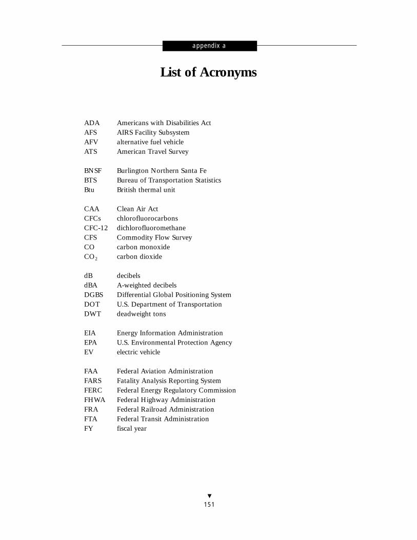
ADA Americans with Disabilities ActAFS AIRS Facility SubsystemAFV alternative fuel vehicleATS American Travel Survey
BNSF Burlington Northern Santa FeBTS Bureau of Transportation StatisticsBtu British thermal unit
CAA Clean Air ActCFCs chlorofluorocarbonsCFC-12 dichlorofluoromethaneCFS Commodity Flow SurveyCO carbon monoxideCO2 carbon dioxide
dB decibelsdBA A-weighted decibelsDGBS Differential Global Positioning SystemDOT U.S. Department of TransportationDWT deadweight tons
EIA Energy Information AdministrationEPA U.S. Environmental Protection AgencyEV electric vehicle
FAA Federal Aviation AdministrationFARS Fatality Analysis Reporting SystemFERC Federal Energy Regulatory CommissionFHWA Federal Highway AdministrationFRA Federal Railroad AdministrationFTA Federal Transit AdministrationFY fiscal year
�
151
List of Acronyms
appendix a

GAO General Accounting OfficeGDD Gross Domestic DemandGDP Gross Domestic ProductGES General Estimates SystemGPRA Government Performance and Results ActGPS Global Positioning System
HAP hazardous air pollutantHMIS Hazardous Materials Information SystemHPMS Highway Performance Monitoring SystemHSR high-speed rail
ICAO International Civil Aviation OrganizationIRI International Roughness IndexISTEA Intermodal Surface Transportation Efficiency ActIT information technologiesITCS Incremental Train Control SystemITD International Trade DivisionITDB Intermodal Transportation DatabaseITS intelligent transportation system
LPG liquefied petroleum gasLTO landing and takeoff
MAC mobile air conditioningMACT maximum achievable control technologyMARAD Maritime Administrationmmtc million metric tons of carbonmpg miles per gallonmph miles per hourMPO metropolitan planning organizationMTBE methyl-tertiary-butyl-ether
N2O nitrous oxideNAFTA North American Free Trade AgreementNET National Emissions TrendsNHTSA National Highway Traffic Safety AdministrationNO2 nitrogen dioxideNOX nitrogen oxidesNPIAS National Plan of Integrated Airport SystemsNPTS Nationwide Personal Transportation SurveyNTAD National Transportation Atlas DatabasesNTI National Toxics Inventory
152 � Transportation Statistics Annual Report 1999

OPEC Organization of Petroleum Exporting CountriesOPS Office of Pipeline SafetyORNL Oak Ridge National Laboratory
PCBs polychlorinated biphenylsPCCIP President’s Commission on Critical Infrastructure ProtectionPM-2.5 particulate matter of 2.5 microns in diameter or smallerPM-10 particulate matter of 10 microns in diameter or smallerPOV privately owned vehiclePSR Present Serviceability RatingPUV personal-use vehicle
quads quadrillion
R&D research and development
SCTG Standard Classification of Transported GoodsSM/N small metropolitan/nonmetropolitanSO2 sulfur dioxide
TEA-21 Transportation Equity Act for the 21st CenturyTEM transportation equipment manufacturingTEU 20-foot equivalent container unitTIUS Truck Inventory and Use SurveyTRB Transportation Research BoardTRDD transportation-related domestic demandTRFD transportation-related final demandTRI Toxics Release InventoryTRRL Transport and Road Research LaboratoryTSAs Transportation Satellite AccountsTSAR Transportation Statistics Annual ReportTSAR98 Transportation Statistics Annual Report 1998TTI Texas Transportation Institute
USACE U.S. Army Corps of EngineersUSCG U.S. Coast GuardUST underground storage tank
vmt vehicle-miles traveledVOC volatile organic compoundsVTS Vessel Traffic Service
Appendix A List of Acronyms � 153

WHO World Health Organization
Y2K Year 2000
ZEV zero-emission vehicle
154 � Transportation Statistics Annual Report 1999

U.S. TO METRIC
Length (approximate)
1 yard (yd) = 0.9 meters (m)1 mile (mi) = 1.6 kilometers (km)
Area (approximate)
1 square mile (sq mi, mi2) = 2.6 kilometers (km2)1 acre = 0.4 hectares (ha) = 4,000 square meters (m2)
Mass/Weight (approximate)
1 pound (lb) = 0.45 kilograms (kg)1 short ton = 2,000 pounds (lbs) = 0.9 metric tons (t)
Volume (approximate)
1 quart (qt) = 0.96 liters (l)1 gallon (gal) = 3.8 liters (l)
Energy Units (approximate)
1 British thermal unit (Btu) = 250 calories = 1,055 joules1 calorie (cal) = 4.186 joules (exactly)1 barrel of oil = 42 U.S. gallons (gal) = 0.16 cubic meters (m3)1 quadrillion Btu (quad) = about 170 million barrels of crude oil
U.S./Metric Conversions and Energy Unit Equivalents
appendix b
�
155

METRIC TO U.S.
Length (approximate)
1 meter (m) = 3.3 feet (ft)1 meter (m) = 1.1 yards (yd)1 kilometer (km) = 0.6 miles (mi)
Area (approximate)
1 square kilometer (km2) = 0.4 square miles (sq mi, mi2)10,000 square meters (m2) = 1 hectare (ha) = 2.5 acres
Mass/Weight (approximate)
1 gram (gm) = 0.036 ounces (oz)1 kilogram (kg) = 2.2 pounds (lb)1 metric ton (t) = 1,000 kilograms (kg) = 1.1 short tons
Volume (approximate)
1 liter (l) = 1.06 quarts (qt)1 liter (l) = 0.26 gallons (gal)
Energy
1 joule = 0.24 calories (cal)1 exajoule = 1018 joules
SOURCE: U.S. Department of Commerce, National Institute of Standards and Technology.
156 � Transportation Statistics Annual Report 1999

AAccidents
aircraft, 84, 85, 86, 88, 89bicycling, 4, 8, 37, 83, 84, 86, 87, 91, 93,
95–96buses, 83, 84, 86, 87, 88, 91, 92–93causes,
alcohol/drug abuse, 8, 88, 94, 95age factors, 7, 94, 95bicycling, 95, 96darkness, 94, 96motor vehicle/pedestrian, 7, 94, 95weather, 8
data needs, 10, 88, 100–101developing countries, 98–99elderly persons, 7, 94gender factors, 98–99injury/exposure, 100light trucks/SUVs, 43, 84, 86, 87, 88, 91,
92–93by mode of transportation, 83motor vehicles, 7, 84
age factors, 7, 94, 95buses, 83, 84, 86, 87, 88, 91, 92–93light trucks, 43, 84, 86, 87, 88, 91,
92–93pedestrians, 7, 84, 86, 93, 94, 95, 96personal-use, 7, 84, 86, 87, 89, 91, 92trucks, 88
pipelines, 85, 86data needs, 8, 100property damage, 124spills, 124, 137
police reports, 96protective devices,
air bags, 88, 90, 134helmets, bicyclists, 96safety belts, 88, 90, 92
rail transportation, 32, 85recreational boating, 84, 85, 86school bus safety, 83, 88, 91, 92–93SUVs, see “light trucks” supratransit, 84, 85; see “buses” suprawaterborne transportation, 84, 85, 86
see also Crashes; Fatalities; Injuries; Transportation safety
Africa, motor vehicle fatalities, 99African-Americans
local travel, 39long-distance travel, 40
Age factorsalcohol abuse, 94children, 7, 39, 40, 41, 83–84, 90–93, 100
fatalities, 90, 91, 92, 94consumer spending, 72–73bicycle fatalities, 95elderly persons, 7, 39, 41, 94, 100fatalities, 7, 90, 91, 92, 94local travel, 39, 41long-distance travel, 40, 41motor vehicle accidents, 7, 94, 95;
see “children” supramotor vehicle age, 20, 31, 33pedestrian fatalities, 7, 94
Agricultural products, 52alcohol fuels, 113, 116, 136food and kindred products, 5, 68, 71
Air bags, 88, 90, 134Air conditioning, motor vehicles (CFCs), 9,
122, 138Aircraft
accidents/fatalities, see “accidents/fatalities” under Air transportation
air pollution, 9, 117, 122, 126, 127, 129, 130–131
Global Positioning Systems, 3, 31–32, 98, 114
data needs, 33, 107energy use, 107, 109freight shipments of, 52icing/deicing, 127 noise, 9, 123, 137number of, 15, 25pollutants,
airborne emissions, 9, 117, 122, 126icing/deicing agents, 127 manufacturing releases, 129, 130–131
terrorism, 97, 98see also Airports; Air transportation
Index
�
157

Airport and Airway Trust Fund, 78Air pollution, 9, 117
aircraft, 9, 117, 122, 126, 127, 129, 130–131ammonia, 118, 119carbon dioxide (CO2), 8, 104, 115–116,
116, 122carbon monoxide (CO), 9, 104, 115–116,
118, 119, 120, 122, 128, 130chlorofluorocarbons (CFCs), 9, 117, 122,
133–134criteria and related pollutants, 9, 116, 117,
119–120, 123, 126–127, 130, 138diesel fuel, 117, 119, 120emission controls, 9, 10, 104, 113–114,
115–116, 121, 132gasoline, 9, 117, 119–120, 121
evaporative emissions, 9, 132global climate change/greenhouse gases, 9,
104, 114–116hazardous, 9, 104, 116, 121–122, 123,
130–131, 136–137lead, 9, 117, 118, 119, 120, 121, 128methane, 114motor vehicles, 8, 9, 117, 129
air conditioning (CFCs), 9, 122, 138emission controls, 9, 10, 104, 113–114,
115–116, 121, 132pollutants released during manufacturing,
128, 129standards, 113–114, 115–116, 121
nitrogen dioxide (NO2), 119, 130nitrogen oxides(NOx), 104, 117, 118, 119,
122, 126, 130nitrous oxide(NO2), 114ozone, ground-level, 120ozone layer depletion, 9, 122, 138
chlorofluorocarbons, 9, 117, 122, 133–134particulate matter, 117, 118, 119, 120, 125pipelines, 9, 122–123sulfur emissions, 117, 119, 123, 128toxic pollutants, 9, 104, 116, 117, 120,
121–122, 123, 125, 126, 127–130,133–138 (passim)
trends, 9, 118, 120volatile organic compounds, 9, 104, 117,
118, 119, 123, 128, 130, 132see also Air quality
AirportsChicago, 51, 125–126condition and performance, 2, 22, 25, 33,
58–59data needs, 33, 126deicing technology, 127District of Columbia, 126–127environmental impacts, general, 10, 127, 137extent and use, 57–58general aviation, 2, 15, 22icing/deicing, 127 Los Angeles, 51New York City, 51, 53noise, 9, 123, 137number and use, 2, 15, 22passenger travel, 15pollution, 125–127runway conditions, 2, 22, 25, 33San Francisco, 51, 127terrorism, 97urban areas, 113–114, 115–116, 121–122,
126see also specific cities
Air quality, 9, 10, 113Clean Air Act, 114, 116, 121, 136, 137electric vehicles, 113standards,
Clean Air Act, 114, 116, 121, 136, 137criteria and related pollutants, 116, 117,
119–120, 123, 126–127, 130, 138electric utilities, 61greenhouse gases, 8, 9, 114motor vehicle emissions, 113–114,
115–116, 121urban, 115–116
trends, 118, 120see also Air pollution
AIRS Facility Subsystem, 122, 137, 138Air taxis, 2, 25, 85, 86, 100Air transportation, 57–59
accidents/fatalities, 7–8, 84, 85, 86, 88, 89air carriers, number of, 2, 15air taxis, 2, 25, 85, 86, 100baggage, lost, 5, 58–59, 145commuter air carriers, 58, 85costs, 37data needs, 33, 107, 126deicing/anti-icing , 127economic indices, 37, 44
158 � Transportation Statistics Annual Report 1999

labor productivity, 6, 76, 77employment, 6, 15, 73, 75, 76, 77energy use, 105extent and use, 2, 13, 22, 25, 57–58freight, 2, 4, 6, 15, 22, 44, 50, 51, 53,
124, 127ton-miles, 15, 44, 46
gender factors, 40general aviation, 2, 15, 22, 25, 84, 85, 86,
88, 89, 100, 119Global Positioning Systems, 31–32government investment, 80government revenues, 78, 79hazardous materials, 124, 127injuries, 85international, 5, 42, 51labor productivity, 6, 76, 77long-distance travel, 2, 4–5, 6, 13, 15, 22,
25, 37, 40, 57–59, 125–127passenger transportation, 2, 4–5, 6, 13, 15,
22, 25, 37, 40, 57–59, 125–127baggage, lost, 5, 58–59, 145commuter, 58, 85passenger-miles, 15, 22, 57, 100
terrorism, 84, 97trends, 2, 5, 85, 89see also Aircraft; Airports; Federal Aviation
AdministrationAlabama, 60, 121Alaska, 28, 60Alcohol and drug abuse
accidents, cause of, 8, 88, 94, 95bicycling accidents, 95motor vehicle drivers, 94, 95pedestrian fatalities, 7, 8, 94
Alcohol fuels, 103, 112–113, 136Alternative and replacement fuels, 8, 111–114,
115–116, 117alcohol fuels, 103, 112–113, 136data needs, 135–136natural gas, 112, 113, 116reformulated gasoline, 112–113, 135–136
Alternative vehicles, 8, 112–113, 115–116, 117, 136
American Public Transit Association, 93Americans with Disabilities Act, 59, 61, 63American Travel Survey, 10, 26, 38, 42, 148Ammonia, 118, 119Amtrak, 2, 5, 16, 22, 23, 24, 64–65, 109Arizona, 5
Army Corps of Engineers, see U.S. Army Corpsof Engineers
Arterial roads, 14, 17, 18, 19, 54, 56Asia
economic decline, 48–49, 110–111motor vehicle fatalities, 99passenger travel to, 42trade with, 4, 48, 50–51see also specific countries
Asians/Pacific Islanders, 41ATS, see American Travel SurveyAviation, see Air transportation
BBaltimore, Maryland, 2, 26, 52, 60Barges, 26, 27, 133Batteries, 113, 131, 134, 138, 138Bicycling, 4, 7, 37, 83, 84, 86, 87, 91, 93,
95–96Biennial Reporting System on Hazardous
Waste, 126Black persons, see African-AmericansBoats, see Ferries; Recreational boating; VesselsBridges, 1, 17, 20, 33, 137Buffalo-Niagara Falls, New York, 53, 126Bureau of the Census
American Travel Survey, 10, 26, 38, 42, 148Commodity Flow Survey, 3–4, 14, 42–49government revenues, 78 (n. 2)international trade, 147National Travel Survey, 36Motor Freight Transportation and
Warehousing Survey, 68Bureau of Economic Analysis, 68Bureau of Labor Statistics, 75Bureau of Transportation Statistics, 143, 144
American Travel Survey, 10, 26, 38, 42, 148capital stock assessments, 81Commodity Flow Survey, 3–4, 14, 42–49National Transportation Atlas Database, 10,
146–148statistical practices, general, 11, 143Transportation Equity Act for the 21st
Century, 10, 144, 146, 147, 148Transportation Satellite Accounts, 6, 68waterborne transportation, 27
Busesaccidents, 83, 84, 86, 87, 88, 91, 92–93bus lanes, 3, 29, 30child safety, 84, 88, 92–93
Index � 159

costs to passengers, 37disabled persons, 63economic indices, 37, 59, 62employment, 6, 75, 76, 77energy use, 105, 136fatalities, 86, 87, 91, 92foreign countries, 84injuries, 86, 87labor productivity, 76, 77long-distance travel, 5, 37, 38number and use, 3, 5, 15, 16, 18, 21, 29,
37, 59revenues, 59route-miles, 29, 30school bus safety, 83, 88, 91, 92–93socioeconomic status of riders, 37urban areas, 16, 29, 37
Business travel, 38, 40, 146see also Commuter rail transportation;
Commuter travel
CCalifornia
freight, 52high-speed rail transportation, 23Los Angeles, 23, 50, 51, 52, 60San Francisco, 23, 51, 60, 127zero emission vehicles, 113
Canada, 4freight, 49, 50, 51–52, 53, 147high-speed rail, 23North American Free Trade Agreement, 52passenger travel, 23, 42
Capital investment, 7, 69, 80GDP, 69labor productivity, 76national accounts, 81see also Government investment
Capital stock, 80–81Carbon dioxide, 9, 104, 115–116, 116, 122Carbon monoxide, 9, 104, 115–116, 118, 119,
120, 122, 128, 130Cargo, see Freight transportationCaribbean, passenger travel to, 42Carpooling, 3, 29, 39, 57, 86, 116
See also vanpoolingCartography, see Maps and mappingCensus Bureau, see Bureau of the CensusCFCs, see Chlorofluorocarbons
CFS, see Commodity Flow SurveyCharleston, South Carolina, 51, 52, 60Chemical and allied products
freight, 47, 62, 64toxic pollutants, 9, 104, 116, 117, 120,
121–122, 123, 125, 126, 127–130,133–138 (passim)
Chicago, Illinoisairports, 51, 125–126high-speed rail, 23–24, 32long-distance travel hubs, 23–24waterborne transportation, 60
Childrenair bags, 90local travel, 39, 41long-distance travel, 40, 41fatalities, 90, 91, 92, 94pedestrians injured, 94risk exposure, data needs, 100safety, 8, 83–84, 88, 90–93, 100safely traveling to and from school, 93school bus safety, 84, 88, 91, 92–93vans, school transportation, 93
China, 111Chlorofluorocarbons, 9, 117, 122, 133–134Cities, see Urban areasClean Air Act, 114, 116, 121, 136, 137Clean Water Act, 133Climate change, see Global climate changeCO, see Carbon monoxideCO2, see Carbon dioxideCoal, freight, 47, 48, 62, 64Coast Guard, see U.S. Coast GuardCoastwise transportation, 25, 26, 59Collector roads, 17, 18, 56Columbia River, 60Commercial transportation,
see Air transportation; Buses; Freighttransportation; Railroads; Waterbornetransportation
Commodities, see Freight transportation; Long-distance freight transportation; specific sectors
Commodity Flow Survey, 3–4, 14, 42–49Communications, see Postal services;
TelecommunicationsCommuter air carriers, 58, 85Commuter rail transportation, 2, 5, 16, 29, 30,
31, 59, 62, 63, 86
160 � Transportation Statistics Annual Report 1999

Amtrak, 2, 5, 16, 22, 23, 24, 64–65, 109Commuter travel, 3, 38–39
air carriers, 58, 85carpools, 3, 29, 39, 57, 86, 116congestion, 5, 10, 53–56, 57, 84ferries, 5, 27, 29, 59, 62time/distance, other than congestion, 38trip chaining, 38vanpools, 3, 29, 86see also Business travel; Commuter rail
transportationComputer systems, 3, 13, 31–32
intelligent transportation systems, 3, 31, 32, 33, 148
Internet, 104rail transportation, 31, 32terrorism, 97see also Databases
Congestion, 5, 10, 53–56, 57, 84carpooling, 3, 29, 39, 57, 86, 116
Conservation, see Alternative and replacement fuels; Environment
Construction sectorairports, 10highway construction, environmental impacts,
131, 137Consumer expenditures on transportation, 5, 6,
67, 68–73demographic factors, 72–73regional factors, 71–72urban/rural, 6, 72
Containers and container ports, 2–3, 26, 50–51Containerships, 2, 26, 27, 28Contaminated materials, see Hazardous materi-
alsCorporate Average Fuel Economy standard,
106, 107Corrective Action Measures (database), 127Cost and cost-benefit factors
air transportation, 37bus transportation, 37data needs, general, 10, 143, 145dredging, 125emission reductions, 104fuel prices, 107, 112hazardous materials spills, 124oil prices, 8, 103, 110–111oil spills, 124passenger transportation, 4, 36–37, 145
personal-use vehicles, 36–37road transportation, congestion, 56, 57Transportation Satellite Accounts, 6, 68
Council for Environmental Quality, 135Courier services, 4, 44–45, 46, 48Crashes
air bags, 88, 90, 134aircraft fatalities, 7, 85, 86, 88, 89alcohol abuse, 88, 94, 95bicyclists, 4, 8, 37, 83, 84, 86, 87, 91, 93,
95–96causes, 8
alcohol/drug abuse, 88, 94darkness, 94, 96
congestion caused by, 56light trucks, 43, 84, 86, 87, 88, 91, 92–93motor vehicles, 8, 84
age factors, 8, 94, 95buses, 83, 84, 86, 87, 88, 91, 92–93light trucks/SUVs, 43, 84, 86, 87, 88, 91,
92–93personal-use, 7, 84, 86, 87, 89, 91, 92trucks, 88
property damage, 101protective devices
air bags, 88, 90, 134helmets, bicyclists, 96safety belts, 88, 90, 92
worldwide data, 98see also Accidents; Fatalities; Injuries
Crime, 83, 90, 101terrorism, 83, 84, 96–98
Criteria and related pollutants, 116, 117, 119–120, 123, 126–127, 130, 138
carbon monoxide (CO), 9, 115–116, 118, 119, 120, 122, 128, 130
carbon dioxide (CO2), 9, 115–116, 122nitrogen dioxide (NO2), 119, 130nitrogen oxides (NOx), 117, 118, 119, 122,
126, 128, 130sulfur dioxide (SO2), 117, 119, 123, 128lead, 9, 117, 118, 119, 120, 121, 128volatile organic compounds, 9, 104, 117,
118, 119, 123, 128, 130, 132Cruise ships, 16, 25, 26Customs Service, see U.S. Customs Service
Index � 161

DDallas-Fort Worth, Texas, freight, 147Dams, see Locks and damsDatabases
hazardous materials, 124, 127–128Intermodal Transportation Database, 10, 144,
146National Transportation Atlas Database, 10,
146–148oil spills, marine, 124pipeline safety, 124rail safety, 32Toxics Release Inventory, 127–128, 133,
137–138Data for Decisions, 144Data needs, 1, 10–11, 32–33, 135–138,
143–148accidents, 8, 88, 98, 100–101aircraft, 33, 107airports, 33, 126air toxics, 116, 136–137alternative and replacement fuels, 135–136capital stock, 81congestion, 54, 55, 56cost factors, 10, 143, 145demographic factors, risk exposure, 100,
143–144economic indices, general, 10, 143, 145, 146,
148employment, wages, 75energy, 107, 135–136, 146environment, 10, 116–117, 126, 136–138,
143, 146fatalities, 100–101freight, 43, 46, 48, 50, 145–146geographic factors, 3, 10, 11, 144hazardous air pollutants, 116, 136–137hazardous materials, general, 127–128, 137highways, 33, 88intelligent transportation systems, 33, 148international, safety data, 8, 84, 97, 98–100international trade, 10, 11, 143, 147local trips, 36long-distance trips, 36motor vehicles, 3, 8, 32–33
disposal, 138fuel economy, 107, 135
noise pollution, 116–117, 137passenger transportation, 36, 144, 145–146
pipelines, 3, 8, 32, 100privacy, 148rail transportation, 88, 132risk exposure, 7–8, 100, 143–144safety, 8, 10, 11, 146, 148
accidents, 8, 88, 98, 100–101risk exposure, 8, 100, 143–144
standards, 136, 137, 138transit, 3, 32–33, 107Transportation Equity Act for the 21st
Century, 10, 144, 146, 147, 148trucking, 136vehicles, 3, 32–33, 107; see “motor vehicles”
suprawaterborne transportation, 11, 33, 100water pollution, 116–117wildlife, 116–117
Defense, see National securityDeicing/anti-icing, 127Delaware River, 60Demographic factors
consumer spending, 72–73data needs, risk exposure, 100, 143–144fatalities, bicyclists and pedestrians, 93marital status, 39, 40Nationwide Personal Transportation Survey,
88 (n. 2), 93passenger travel, 37, 38race/ethnicity, 39–41, 143–144transit, 29see also Age factors; Households; Rural areas;
Socioeconomic status; Urban areasDepartments of U.S. Government, see headings
beginning “U.S. Department of…”Detroit, Michigan
freight, 53, 60high-speed rail, 23, 32waterborne transportation, 60
Developing countries, safety, 98–100Diesel fuel, 117, 119, 120Disabled persons, transit services, 31, 53,
59–60, 63District of Columbia,
airports, 126–127high-speed rail, 23, 24
Dredging, 9, 125, 137Drivers’ licenses, see Licenses and licensingDrug abuse, see Alcohol and drug abuseDulles Airport, 126–127
162 � Transportation Statistics Annual Report 1999

E Eastern U.S., oceanborne international trade,
4, 50, 51see also specific states
Economic factors, 1, 4, 5–8, 67–82Asia, 8, 48–49, 110–111capital investment, 1, 7, 69, 76, 80, 81for-hire transportation, 6, 68freight, 44–48 (passim)
GDP, 4, 44, 45, 48, 68international, 4, 10, 44, 48–53revenues, 2, 6, 21, 61–62
gasoline, 8, 69, 72, 111fuel economy, 8, 104, 105–109, 115, 135
GDP, 5–6, 67–71, 148energy use, 105freight transportation, 4, 44, 45, 48, 68international trade, 4transportation-related final demand, 5–6,
67–68, 69, 78globalization, 10, 144, 147global warming, 114in-house transportation, 6, 68international trade indices, 4, 5–6, 48–49Japan, 111labor productivity, 6, 53, 64, 76–77oil imports, 8, 104, 109–111passenger transportation indices, 39–42,
88 (n. 2), 144productivity, 5, 10, 53, 64, 67, 74, 76–77property damage, 8, 53, 61, 100, 101, 124,
146rail transportation indices, 2, 6, 21, 61–65Russia, 110transportation expenditures, 5, 6
capital investment, 1, 7, 69, 76, 80, 81consumer expenditures on transportation,
5, 6, 67, 68–73government expenditures, 5, 7, 23, 67, 69,
78, 79–81, 145transportation-related final demand, 5–6,
67–68, 69, 78transportation revenues,
air transportation, passengers, 57buses, 59government revenues, 5, 6–7, 67, 78–79rail freight, 2, 6, 21, 61–62rail, passenger, 59transit, 59, 61, 62
Transportation Satellite Accounts, 6, 68trucking, general, 14, 44, 45, 46, 68value-added, general, 44, 68wages and salaries, 74, 75see also Cost and cost-benefit factors;
Employment; International trade;Socioeconomic status; specific sectors
EIA, see Energy Information AgencyElderly persons
fatalities, 7, 94local travel, 39, 41long-distance travel, 40, 41motor vehicle drivers, 7pedestrians, 7, 94risk exposure, data needs, 100
Electric vehicles, 113, 116, 136El Paso, Texas, 53Emergency medical services, see Medical servicesEmission controls, 8–9, 10, 104, 113–114,
115–116, 121, 132Employment, 67, 73–76
air transportation, 6, 15, 73, 75, 76, 77bus transportation, 6, 75, 76, 77business travel, 38, 40, 146; see also
Commuter traveldata needs, wages, 75for-hire transportation, 6, 73–74freight, 45
trucking, 6, 73–74, 75, 76, 77warehousing, 6, 73–74
labor force participation, 4, 37, 74labor productivity, 5, 6, 53, 64, 67, 74,
76–77local travel, 73, 74; see also Commuter travelmotor vehicle operators, general, 75; see
“bus transportation” supraby mode/occupation, 73, 75passenger travel, increases in, 37pipelines, 73, 74, 76, 77rail transportation, 16, 21, 73, 74, 75, 76service industries, general, 73, 74transit, 16, 75, 76, 77trip purpose, 38; see also Business traveltrucking, 6, 73–74, 75, 76, 77wages and salaries, 74, 75warehousing, 6, 73–74waterborne transportation, 73, 75
Energy Information Administration, 104 (n. 1), 111
Index � 163

Energy resources see Coal; Natural gas; OilEnergy use/efficiency, 1, 8, 54
aircraft, 107, 109congestion, 56, 57data needs, 107, 135–136, 146fuel economy standards, 8, 56, 105, 106, 107light trucks, 8, 105, 106–107, 109, 135motor vehicles, general, 8, 56, 57, 104,
105–109, 115, 135personal-use vehicles, 8, 56, 57, 104,
105–107, 109technological innovations, 8, 104, 107trucks, 105, 106–107, 136see also Alternative and replacement fuels;
Diesel fuel; GasolineEnvironment, 1, 8–10, 104, 116–135, 136–138
airports, general, 9, 127, 137data needs, 10, 116–117, 126, 136–138, 143,
146habitat, 9, 125, 116–117highway construction, 131, 137sediment, dredged, 9, 125, 137transit, 116transportation infrastructure development
impacts, 9, 124–127, 131, 137see also Air pollution; Air quality; Hazardous
materials; Noise; Pollution; Wastematerials
Environmental Protection Agencyairport deicing, 127air quality, 8, 9, 117, 119
CFCs, 122criteria and related pollutants, 116, 117,
119–120, 123, 126, 127–130, 138toxic pollutants, 120–122, 126, 127–130
gasoline, evaporative emissions, 9, 132highway and bridge construction debris, 137National Emission Trends, 117, 120,
126–127, 132, 136, 137National Toxics Inventory, 120, 128,
136–137noise, 123oil and gas pipeline emissions, 122–123pipelines, 137toxics, 120–122, 126, 127–130, 132, 133,
135National Toxics Inventory, 120, 128,
136–137Toxics Release Inventory, 127–128, 133,
137–138
transportation equipment cleaning, 133underground storage tanks, 127, 132–133vessel dismantling, 135
Ethanol, 112, 116Europe
air freight, 51passenger travel to, 42road safety, 98see also specific countries
Expenditures, see Consumer transportation expenditures; Cost and cost-benefit factors;Transportation expenditures
Exports and imports, see International transportation; International trade
FFatalities, 7–8
age factors, 7, 90, 91, 92, 94air transportation, 7–8, 84, 85, 86, 88, 89bicyclists, 8, 84, 93, 94, 95bus accidents, 86, 87, 91, 92causes,
alcohol/drug abuse, 8, 88, 94, 95age factors, 7, 94, 95bicycling, 95, 96darkness, 94, 96motor vehicle/pedestrian, 8, 94, 95
children, 90, 91, 92, 94data needs, 100–101developing countries, 98–99DOT policy, 7, 83elderly persons, 7, 94gender factors, 98–99highways, 84, 85, 87, 88; see also “motor
vehicles” infrainternational data, by country, 99by mode, 7–8, 85–88, 89, 91by occupant/nonoccupant category, 87motor vehicles, 7–8, 85, 86, 93, 94
bicyclists struck by, 7, 8, 83, 84, 86, 91,93, 94
causes, 7, 8, 94, 95developing countries, 99light trucks, 7, 84, 86, 87, 89, 91, 93motorcyclists, 84, 87, 88, 89, 91pedestrians, 7–8, 84, 86, 93, 94
personal-use vehicles, 7, 84, 86, 87, 89, 91, 92
pipelines, 8, 85, 100, 124, 137recreational boating, 84, 85, 86
164 � Transportation Statistics Annual Report 1999
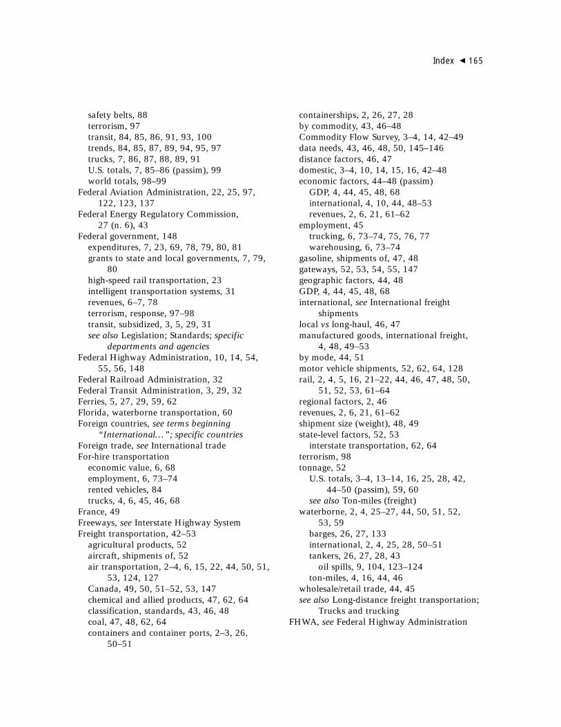
safety belts, 88terrorism, 97transit, 84, 85, 86, 91, 93, 100trends, 84, 85, 87, 89, 94, 95, 97trucks, 7, 86, 87, 88, 89, 91U.S. totals, 7, 85–86 (passim), 99world totals, 98–99
Federal Aviation Administration, 22, 25, 97, 122, 123, 137
Federal Energy Regulatory Commission, 27 (n. 6), 43
Federal government, 148expenditures, 7, 23, 69, 78, 79, 80, 81grants to state and local governments, 7, 79,
80high-speed rail transportation, 23intelligent transportation systems, 31revenues, 6–7, 78terrorism, response, 97–98transit, subsidized, 3, 5, 29, 31see also Legislation; Standards; specific
departments and agenciesFederal Highway Administration, 10, 14, 54,
55, 56, 148Federal Railroad Administration, 32Federal Transit Administration, 3, 29, 32Ferries, 5, 27, 29, 59, 62Florida, waterborne transportation, 60Foreign countries, see terms beginning
“International…”; specific countriesForeign trade, see International tradeFor-hire transportation
economic value, 6, 68employment, 6, 73–74rented vehicles, 84trucks, 4, 6, 45, 46, 68
France, 49Freeways, see Interstate Highway SystemFreight transportation, 42–53
agricultural products, 52aircraft, shipments of, 52air transportation, 2–4, 6, 15, 22, 44, 50, 51,
53, 124, 127Canada, 49, 50, 51–52, 53, 147chemical and allied products, 47, 62, 64classification, standards, 43, 46, 48coal, 47, 48, 62, 64containers and container ports, 2–3, 26,
50–51
containerships, 2, 26, 27, 28by commodity, 43, 46–48Commodity Flow Survey, 3–4, 14, 42–49data needs, 43, 46, 48, 50, 145–146distance factors, 46, 47domestic, 3–4, 10, 14, 15, 16, 42–48economic factors, 44–48 (passim)
GDP, 4, 44, 45, 48, 68international, 4, 10, 44, 48–53revenues, 2, 6, 21, 61–62
employment, 45trucking, 6, 73–74, 75, 76, 77warehousing, 6, 73–74
gasoline, shipments of, 47, 48gateways, 52, 53, 54, 55, 147geographic factors, 44, 48GDP, 4, 44, 45, 48, 68international, see International freight
shipmentslocal vs long-haul, 46, 47manufactured goods, international freight,
4, 48, 49–53by mode, 44, 51motor vehicle shipments, 52, 62, 64, 128rail, 2, 4, 5, 16, 21–22, 44, 46, 47, 48, 50,
51, 52, 53, 61–64regional factors, 2, 46revenues, 2, 6, 21, 61–62shipment size (weight), 48, 49state-level factors, 52, 53
interstate transportation, 62, 64terrorism, 98tonnage, 52
U.S. totals, 3–4, 13–14, 16, 25, 28, 42, 44–50 (passim), 59, 60
see also Ton-miles (freight)waterborne, 2, 4, 25–27, 44, 50, 51, 52,
53, 59barges, 26, 27, 133international, 2, 4, 25, 28, 50–51tankers, 26, 27, 28, 43
oil spills, 9, 104, 123–124ton-miles, 4, 16, 44, 46
wholesale/retail trade, 44, 45see also Long-distance freight transportation;
Trucks and truckingFHWA, see Federal Highway Administration
Index � 165

G Gas, see Natural gasGasoline, 103
air pollution, 10, 117, 119–120, 121evaporative emissions, 10, 132
economic indices, 8, 69, 72, 111; see “fuel economy” infra
freight shipments of, 47, 48fuel economy, 8, 9, 104, 105–109, 115, 135reformulated, 112–113, 135–136taxes, 7, 78, 135underground storage tanks, 10, 132–133see also Alternative and replacement fuels
GDP, see Gross Domestic ProductGender factors
local trips, 38, 39long-distance travel, 40passenger mobility patterns, 39–40road accidents, injuries and fatalities, 98–99
General Accounting Office, see U.S. General Accounting Office
General aviation, 2, 15, 22, 25, 84, 85, 86, 88, 89, 100, 119
Global Positioning Systems, 3, 31–32Geographic factors
data needs, 3, 10, 11, 144freight, 44, 48international trade, domestic transportation
of, 10, 44, 143, 147long-distance travel, 42oil, geopolitical factors, 109–110passenger travel, 41–42transit, 59see also Maps and mapping; Regional factors;
Rural areas; Suburban areas; Urbanareas; specific regions
Geographic information systems, 3Georgia, high-speed rail, 24Germany, 28, 49Global climate change, 9, 104, 114–116Global Positioning Systems, 3, 31–32, 98, 114Government expenditures, 5, 7, 67, 69, 78,
79–81, 145federal, 7, 23, 69, 78, 79, 80, 81local, 7, 69, 79, 80, 81state, 7, 69, 79, 80, 81
Government investment, 80–81Government Performance and Results Act, 144Government revenues, 5, 6–7, 67, 78–79
federal, 7, 78highways, 7, 78, 79inflation, impact on, 78local, 7, 78–79by mode, 78, 79state, 7, 78–79, 80, 135taxes, 7, 78–79, 135waterborne transportation, 78–79
Government role, see Federal government; Local government; State government
GPRA, see Government Performance and Results Act
Great Lakes, 16, 28, 59ports, 2, 16, 25, 26, 125
Greece, 28Greenhouse gases, 8, 104, 114–116
Kyoto Protocol, 8, 114see also specific gases
Gross Domestic Product, 5–6, 67–71, 148energy use, 105freight transportation, 4, 44, 45, 48, 68international trade, 4, 69motor vehicles, 69transportation-related final demand, 5–6,
67–68, 69, 78Gulf ports, 50, 51
HHabitat, see WildlifeHandicapped persons, see Disabled personsHarbors and ports, see Ports; specific citiesHawaii, 60, 121Hazardous air pollutants, 9, 104, 116, 121–122,
123, 130–131, 136–137Hazardous materials, 10, 104, 116–117,
126–127air transportation, 124, 127costs of spills, 124databases, 124, 127–128data needs, 127–128, 137dredged sediment, 9, 125, 137pipeline accidents/injuries/fatalities, 85, 124rail transportation, 124, 132road transportation spills, 9, 124spills, 123–124standards, 130–131state government, 127, 132, 133state-level trends, 120–121storage tanks, leakage, 10, 127, 132–133
166 � Transportation Statistics Annual Report 1999

vehicle and parts manufacturing, 127–130, 137–138
vehicle disposal, 133–134, 138waterborne transportation, 124
vessel dismantling, 134–135see also Hazardous air pollutants; Toxic
pollutantsHazardous Materials Information System, 124,
127Helmets, bicyclists, 96HFCs, see HydrofluorocarbonsHigh-speed rail transportation, 14, 22, 23–24,
32Highway Performance Monitoring System, 54Highways, 14, 15, 17–20
accidents, 85bridges, 1, 17, 20collector, 17, 18, 56condition and performance, 1, 14, 17, 18–19,
21, 33developing countries, 99, 100
construction and materials, environmental impacts, 131, 137
data needs, 33, 88extent and use, 14, 15, 17fatalities, 7, 84, 85, 87, 88; see also “motor
vehicles” under FatalitiesFHWA, 10, 14, 54, 55, 56, 148government investment, 81government revenues, 78, 79government spending, 7, 80injuries, 85; see also “motor vehicles” under
Injuriesintelligent transportation systems, 31Interstate Highway System, 14, 15, 17, 18,
19, 54, 56rail crossings, 23, 31rural, 14, 17, 19, 21
vehicle-miles traveled, 5, 54, 56urban, 3, 5, 14, 15, 17, 18, 19, 21, 54–56see also Motor vehicles; Trucks and trucking
Highway Trust Fund, 7Highway vehicles
asphalt and concrete, manufacturing emissions, 131
energy consumption, 104, 105–106fatalities, 7, 84, 85, 87, 88hazardous materials spills, 9, 124number and use, 1–2, 15, 17–18, 21
vehicle-miles traveled, 15, 54see also Motor vehicles; Trucks and trucking
Hispanicslocal travel, 39, 41long-distance travel, 40, 41
Hong Kong, 99Households, 5, 6
consumer spending, general, 68, 71–73income, 37, 39, 40–42, 68motor vehicle ownership, 18, 20, 37passenger travel, 37, 39, 40–41
trip chaining, 38Houston, Texas, 5, 51, 52, 55Hydrofluorocarbons (HFCs), 122, 138
I Icing, aircraft, see Deicing/anti-icingIllinois, 32, 52
see also Chicago, IllinoisImports and exports, see International
transportation; International tradeIncome, see Socioeconomic statusIncremental Train Control System, 32Indiana, 52, 60Information technology, see Computer systemsIn-house transportation, 6, 68Injuries, 83
air bags, causing, 90air transportation, 85bicyclists, 94, 95data needs, 8, 10, 100, 146elderly persons, 94gender factors, 98–99medical services, 88, 95, 97by mode, 86, 87motor vehicles, 84, 94
air bags, 90pedestrians, 94
rail transportation, 85transit, 85trucks, 7, 86, 87, 88, 89, 91U.S. totals, 85, 87worldwide totals, 98–99see also Fatalities
Inland waterwayscondition and performance, 59dredging, 9, 125, 137extent and use, 2, 16, 25, 59fuel tax, 78–79
Index � 167

locks and dams, 25, 59recreation and tourism, 25see also Great Lakes; Ports; Vessels
Integrated Pipeline Information System, 124Integrated Urban Toxics Strategy, 121–122Intelligent transportation systems, 3, 14, 31, 32,
33, 148Intermodal/multimodal transportation, 2,
25–26, 43–44, 50, 53, 62, 64containers and container ports, 2–3, 26,
50–51containerships, 2, 26, 27, 28database, 10, 144, 146data needs, 144, 146, 147
Intermodal Surface Transportation Efficiency Act (ISTEA), 23, 144
Intermodal Transportation Database, 10, 144, 146
International agreementsgreenhouse gases, Kyoto Protocol, 8, 114Marine Pollution Convention, 125North American Free Trade Agreement, 52ozone layer depletion, 138
International Federation of Red Cross and Red Crescent Societies, 98
International freight shipments, 10, 25, 48–53air, 50, 51by country, 49data needs, 50domestic activity and, 10, 44, 143, 147gateways, 52, 53, 54, 55, 147by mode, 51ports, 50–51, 52, 53, 54, 55, 147rail, 50, 51, 52trucking, 51, 52, 53value of goods, 49–50U.S. merchandise trade, 4, 48, 49–53waterborne, 4, 25, 28, 50–51
International long-distance trips, 4–5, 42International perspectives
aircraft noise, 123developing countries, safety, 98–100global climate change, 8, 104, 114–116safety, 7–8, 84, 97, 98–100terrorism, 97
International Roughness Index, 14International trade, 4, 48–53
Asia, 4, 48, 50–51; see also specific countriescontainer ports, 2, 26, 50–51data needs, 10, 50, 143, 147
domestic transportation of, 10, 44, 143, 147eastern U.S., 50, 51economic indices, general, 5–6, 48–49GDP and, 4, 69globalization, 10, 144, 147motor vehicles, 6, 52, 128North American Free Trade Agreement, 52oil, 8, 104, 109–111Pacific Rim, 4, 48, 50–51U.S. Customs Service, 147U.S. merchandise trade, 4, 48, 49–53see also specific countries
International transportationair transportation, 5, 42, 51freight, see International freight shipmentsgateways, 52, 53, 54, 55, 147U.S. Customs Service, 147waterborne, 2, 4, 25, 28, 50–51
Internet, 104Interregional freight transportation, 46Interstate freight transportation, 62, 64Interstate Highway System
condition, 14, 17, 18, 19extent and use, 15, 54, 56
Intoxication, see Alcohol and drug abuseIntraregional freight transportation, 46Investment, see Capital investmentISTEA, see Intermodal Surface Transportation
Efficiency Act (ISTEA)ITS, see Intelligent transportation systems
JJapan, 28, 49, 51, 84, 99, 111
KKennedy International Airport, 51, 53Kyoto Protocol, 8, 114
LLabor, see Employment; ProductivityLaredo, Texas, 53Lead, 9, 117, 118, 119, 120, 121, 128, 134Leaking underground storage tanks, 10, 127,
132–133Legislation
Americans with Disabilities Act, 59, 61, 63Clean Air Act, 114, 116, 121, 136, 137Clean Water Act, 133Kyoto Protocol, congressional approval, 114
168 � Transportation Statistics Annual Report 1999

Government Performance and Results Act, 144
Intermodal Surface Transportation Efficiency Act (ISTEA), 23, 144
Rail Passenger Service Act, 22Transportation Equity Act for the 21st
Century (TEA–21), 10, 23, 83–84, 144, 146, 147, 148
Leisure, see Recreational activities; Recreationalboating
Licenses and licensing, driversdeveloping countries, driver training, 100number of, 37
Light trucksaccidents, 43, 84, 86, 87, 88, 91, 92–93data needs, 135energy efficiency, 8, 105, 106–107, 109, 135injuries/fatalities, 7, 84, 86, 87, 89, 91, 93number and use, 1–2, 8, 15, 106–107, 108pollutants released during manufacturing,
131sport utility vehicles, 1–2, 17, 84, 91, 105,
108Liquefied petroleum gas, 111–112Local government, 7, 38, 69, 78–79, 80, 81Local roads
bridges, 17vehicle-miles traveled, 56
Local travel, 4, 13, 35–37African-Americans, 39age factors, 39, 41defined, 35employment, 73, 74; see also Commuter
travelgender factors, 38, 39household income, 37, 41–42by mode, 37passenger-miles, 35–36, 37, 41purpose, 38; see also Commuter travelrail, 2, 16, 37; see also Commuter rail
transportationtrip chaining, 38walking as a form of transportation, 4, 8, 37,
84, 90, 91, 93–95; see also PedestriansLocks and dams, 25, 59Long Beach, California
international freight, 50–51port facilities, 2, 26, 50–51, 52, 60
Long-distance freight transportation, 46
agricultural products, air, 2, 4, 6, 15, 22, 44, 50, 51, 53, 124, 127Canada, 49, 50, 51–52, 53, 147chemical and allied products, 47, 62, 64coal, 47, 48, 62, 64containers and container ports, 2, 26,
50–51containerships, 2, 26, 27, 28by commodity, 47economic factors, 4, 10, 44, 48–53international; see International freight
shipmentsinterstate, 62, 64manufactured goods, 48, 49, 52Mexico, 49, 50, 51–52, 53, 147minerals, 47, 48, 64by mode, 44, 51rail, 44ton-miles, 15, 44, 46, 51, 62, 64see also Commodity Flow Survey
Long-distance travel (trips), 4, 13, 35African-Americans, 40age factors, 40, 41air transportation, 2, 4, 6, 13, 15, 22, 25, 37,
40, 57–59, 125–127American Travel Survey, 38, 42buses, 5, 37, 38business, 38, 40children, 40, 41cost factors, 37domestic, 36elderly persons, 40, 41extent of, 35, 36, 38, 40, 41gender factors, 40geographic factors, 42Hispanics, 40, 41income factors, see “socioeconomic status”
infrainternational, 42by mode, 37Nationwide Personal Transportation Survey,
38personal-use vehicles, 36–37, 40purpose of, 38, 40race/ethnicity, 40, 41rail transportation, 5, 37, 38socioeconomic status, 40, 41trends, 35, 36
Los Angeles, California
Index � 169

airports, 51high-speed rail, 23waterborne transportation, 50, 51, 52, 60
Louisiana, 51, 60LPG, see Liquefied petroleum gasLumber and wood products
alcohol fuels, 113freight shipments, 47international trade, 52
MMail, see Postal servicesMaintenance and repair, pollutant emissions,
131–133Manufactured goods, 47
international freight, 4, 48, 49, 52U.S. merchandise trade, 48, 49, 49–53vehicles and vehicle parts, pollutants, 10,
117, 127–131, 137–138Maps and mapping
airports, enplanements, 58 freight
gateways, 55rail networks, 63ports, 54, 60
high-speed rail corridors, 24transit markets, 61
Marine Pollution Convention, 125Marine vessels
containerships, 2, 26, 27, 28cruise ships, 16, 25, 26dismantling, 134–135recreational boats, 2, 16, 25, 84, 85, 86,
129, 131tankers, 26, 27, 28, 43
oil spills, 9, 104, 123–124Maritime Administration, 27, 28, 134–135Maritime transportation, 2, 4
accidents, 84, 85, 86coastwise transportation, 25, 26, 59cruise ships, 16, 25, 26data needs, 11extent and use, 2, 16, 25–27freight, 2, 4, 25–27, 44, 50, 51, 52, 53, 59
containers and container ports, 2–3, 26, 50–51
containerships, 2, 26, 27, 28tankers, 26, 27, 28, 43
oil spills, 9, 104, 123–124
see also Ports; VesselsMaryland, 2Massachusetts, 60Mass transit, see TransitMedical services
accidental injuries, 88, 95terrorism, 97
Men, see Gender factorsMethane, 114Methanol, 112–113Mexico, 4
freight, 49, 50, 51–52, 53, 147North American Free Trade Agreement, 52passenger travel, 42
Miami, Florida, international freight, 52, 60Michigan
freight, 52, 53, 60high-speed rail, 23, 32waterborne transportation, 60
Mid-range travel (trips), 11Midwest U.S.
consumer spending, 71high-speed rail, 23see also specific states
Minerals and mining, 47, 48, 64coal, 47, 48, 62, 64
Minnesota, 60Minority groups, see Race/ethnicity;
specific groups Missouri, 60Mobility
database on, 10factors associated with, 39–42
Modified Marine Safety Information System, 124
Motorcycles, 15, 18, 21, 84, 87, 88, 89, 91, 123Motor Freight Transportation and Warehousing
Survey, 68Motor oil, 134Motor vehicles
accidents, 7, 84age factors, 7, 94, 95buses, 83, 84, 86, 87, 88, 91, 92–93light trucks/SUVs, 43, 84, 86, 87, 88, 91,
92–93pedestrians, 7, 84, 86, 93, 94, 95, 96personal-use, 84, 86, 87, 89, 91, 92trucks, 88
age of vehicle, 20, 31, 33
170 � Transportation Statistics Annual Report 1999
air bags, 88, 90, 134air pollution, 9, 117, 129
air conditioning (CFCs), 9, 122, 138emission controls, 8, 10, 104, 113–114,
115–116, 121, 132pollutants released during manufacturing,
128, 129standards, 113–114, 115–116, 121
alcohol/drug abuse by drivers, 94, 95alternative vehicles, 8, 112–113, 115–116availability of, 36–37batteries, 113, 131, 134, 138, 138consumer spending, 69, 71, 72–73data needs, 3, 8, 32–33
disposal, 138fuel economy, 107, 135
elderly drivers/pedestrians, 8, 94electric vehicles, 8, 113, 116, 136employment of operators, 75
bus transportation, 6, 75, 76, 77energy consumption/efficiency, 8, 56, 57,
104, 105–109, 115, 135fatalities, 7–8, 85, 86, 93, 94
bicyclists struck by, 8, 83, 84, 86, 91, 93, 94
causes, 7, 94, 95developing countries, 99light trucks, 7, 84, 86, 87, 89, 91, 93motorcyclists, 84, 87, 88, 89, 91pedestrians, 7, 84, 86, 93, 94
freight, shipment of motor vehicles, 52, 62, 64, 128
fuel taxes, 7, 78, 135GDP, 69injuries, 84, 94
air bags, causing, 90pedestrians, 94
international trade in, 52, 128motor oil, maintenance spills, 131noise pollution, 9, 123, 137number of, 1–2, 13, 15, 17–18, 98, 106–107ownership, household, 18, 20, 37personal consumption, 6pollutants, manufacturing phase, 117,
127–131recycling of waste, 133safety belts, 88, 90, 92taxis, 75, 84, 91
technological innovations, 112–113, 115–116, 117, 136
vans,fuel economy, 109number of, 108used in school transportation, 93vanpooling, 3, 29, 86
vehicle-miles traveled, 5, 8, 15, 56air pollution, 117, 119data needs, 100fatalities, 7, 84by functional class, 56personal-use vehicles, 37, 39
see also Buses; Diesel fuel; Gasoline; Highway vehicles; Personal-use vehicles; Roadtransportation; Trucks and trucking
Multimodal transportation, see Intermodal/multimodal transportation
NNAFTA, see North American Free Trade
AgreementNational Academy of Sciences, 143National accounts, 81 National Airspace Commission, 98National Defense Reserve Fleet, 135National Emission Trends, 117, 120, 126–127,
132, 136, 137National Highway System, 15National Highway Traffic Safety
Administration, 84, 90, 92National Industry-Occupation Employment
Matrix, 75National Occupant Protection Use Survey, 90National Plan of Integrated Airport Systems,
22, 25National Railroad Passenger Corporation,
see AmtrakNational Research Council, 10National security
government expenditures, 69National Defense Reserve Fleet, 135oil supply, 104, 109–111waterborne transportation, 28
National Toxics Inventory, 120, 128, 136–137National Transportation Atlas Database, 10,
146–148National Transportation Safety Board, 92, 93,
124
Index � 171
National Travel Survey, 36Nationwide Personal Transportation Survey, 10,
18, 20, 35, 36, 37, 38, 41, 55, 56–57, 88,93, 148
Natural gasas alternative fuel, 112, 113, 116energy use, 100liquefied petroleum gas, 111–112pipelines, 3, 6, 9, 13, 17, 27, 76, 85, 86, 103,
122–123, 124accidents/injuries/fatalities, 8, 85, 86, 124,
137Navigational aids, Global Positioning Systems,
3, 31–32, 98Netherlands, 49, 99New Jersey
freight, 51, 52, 60waterborne transportation, 51, 52, 60
New York Cityairports, 51, 53Canadians, trips to, high-speed rail, 23waterborne transportation, 51, 52, 60
New York Statefreight, 51, 52, 60high-speed rail, 23zero emission vehicles, 113–114
Nitrogen dioxide (NO2), 119, 130Nitrogen oxides (NOx), 104, 117, 118, 119,
122, 126, 130Nitrous oxide (N2O), 114Noise
aircraft, 9, 123, 137data needs, 116–117, 137motor vehicle traffic, 9, 123, 137railroad vehicles, 123, 137
Nonhazardous industrial wastes, 9, 130Norfolk, Virginia, 51, 52, 60North America, see Canada; Mexico; Regional
factors, specific U.S. cities and statesNorth American Free Trade Agreement, 52North American Interchange on Transportation
Statistics, 11, 148North American Transportation Statistics
Project, 147North Carolina, 24, 52Northeast U.S.
consumer spending, 71–72high-speed rail transportation, 23, 24see also specific states
O Oakland, California, 52Oak Ridge National Laboratory, 43Ocean transportation, see Maritime
transportationOffice of Pipeline Safety, 27 (n. 6), 124O’Hare Airport, 125–126Ohio, 52, 60Oil, 3, 9, 103
consumption, 8, 103, 104, 110, 111fuel economy standards, 8, 56, 105, 106,
107highway vehicles, 8, 56, 57, 104,
105–109, 115, 135foreign sources, 8, 104, 109–111freight, 43, 51; see also “waterborne
transportation (tankers)” infra international transportation, 28, 51, 52labor productivity, 76, 77motor oil, 135pipelines, 3, 6, 9, 13, 17, 27, 76, 85, 86, 103,
122–123, 124prices, 103, 104spills, 9, 104, 123–124Strategic Petroleum Reserve, 104, 110supply, 8, 103, 104, 109–111waterborne transportation (tankers), 9, 26,
27, 28, 43, 104, 123–124Oil spills, 9, 104, 123–124On-time performance, 57, 58Oregon, 23, 32Organization of Petroleum Exporting Countries,
109–110Otay Mesa, California, 53Ozone, ground–level, 120Ozone layer, 9, 122, 138
chlorofluorocarbons, 9, 117, 122, 133–134
PPacific Rim, trade with, 4, 48, 50–51Pacific states, high-speed rail, 23Parcels, see Courier services; Postal servicesParking lots, accidents, 94Particulate matter, 117, 118, 119, 120, 125Passenger-miles, 4, 6, 7, 76
air pollutants, 116air transportation, 15, 22, 57, 100
172 � Transportation Statistics Annual Report 1999
European road transportation, 98geographic origin of travelers, 42household income, 41local travel, 35–36, 37, 41long-distance travel, 36, 41racial/ethnic factors, 41rail transportation, 109by mode, 37transit, 3, 5, 16, 59U.S. total, 13, 35, 36waterborne, 16
Passenger transportation, 4, 35–42air, 2, 4–5, 6, 13, 15, 22, 25, 37, 40, 57–59,
125–127baggage lost, 5, 58–59, 145commuter, 58, 85passenger-miles, 15, 22, 57, 100
business travel, 38, 40, 146Canada, 23, 42Caribbean, 42congestion, 5, 10, 53–56, 57, 84
carpooling, 3, 29, 39, 57, 86, 116costs of, 4, 36–37, 145data needs, 36, 144, 145–146distance, see Local travel; Long-distance
travel (trips); Mid-range travel (trips);Passenger-miles
demographic/socioeconomic factors, 39–42, 88 (n. 2), 144
economic indices, 39–42, 88 (n. 2), 144energy use and, 104, 105, 107, 109household-related data, 37, 39, 40–41
income, 39, 40–41, 68trip chaining, 38
Mexico, 42mid-range travel (trips), 11miles of, U.S. total, 13, 35, 36Nationwide Personal Transportation Survey,
10, 18, 20, 35, 36, 37, 38, 41, 44,56–57, 88, 93
purpose, 38rail, 5, 22
Amtrak, 2, 5, 16, 22, 23, 24, 64–65, 109commuter rail transportation, 2, 5, 16, 29,
30, 31, 59, 62, 63, 86high-speed rail transportation, 14, 22,
23–24, 32rural areas, 39, 42
transit, 3, 32–33
school children, 83, 88, 90–93socioeconomic status and, 4, 37
local, 38, 39long-distance, 40, 41
urban areas, 39, 40, 41–42; see “congestion” supra
waterborne, 16, 25, 26–27cruise ships, 16, 25, 26ferries, 27, 29, 59, 62
see also Buses; Commuter rail transportation; Commuter travel; Local travel; Long-distance travel (trips); Personal-use vehicles; Transit
Pedalcyclists, see BicyclistsPedestrians, 83, 93–95, 100
accidents/injuries, 7, 84, 86, 93, 94, 95, 96alcohol abuse by, 8, 94bicycling on sidewalks, 96developing countries, safety, 100elderly, 7, 94fatalities, 7, 8, 84, 86, 93, 94
age factors, 8, 94see also Walking as a form of transportation
Pennsylvania, 52Performance Monitoring System, 59Personal-use vehicles, 4, 36–37
accidents/fatalities, 84, 86, 87, 89, 91, 92age of motor vehicle, 20, 31, 33air bags, 88, 90, 134availability of, 36–37bicycles, 4, 8, 37, 83, 84, 86, 87, 91, 93,
95–96carpooling, 3, 29, 39, 57, 86, 116child safety, 88, 92cost of, 36–37energy efficiency, 8, 56, 57, 104, 105–107,
109gender factors, 39government revenues, 79households owning, 18, 20, 37injuries, 87long-distance travel, 36–37, 40motorcycles, 15, 18, 21, 84, 87, 88, 89,
91, 123number of, 1–2, 15, 18, 20, 21, 98, 106–107,
108recycling of waste, 133safety, 88, 90trip chaining, 38
Index � 173
vehicle-miles traveled, 37, 39see also Light trucks
Petroleum and petroleum products, see Gasoline; Motor oil; Natural gas; Oil
Phoenix, Arizona, 5, 55Pipelines,
accidents/fatalities, 85, 86data needs, 8, 100property damage, 124spills, 124, 137
air pollution, 8, 9, 122–123data needs, 3, 8, 32, 100economic indices, 44employment, 73, 74, 76, 77energy use, 105extent, use, and performance, 3, 4, 17, 27,
44, 51government revenues, 78government spending, 7, 80hazardous materials, accidents/injuries/
fatalities, 85, 124labor productivity, 6, 76, 77oil and gas, 3, 6, 9, 13, 17, 27, 76, 85, 86,
103, 122–123, 124Police accident reports, 96Political factors, foreign oil supply, 8, 104, 110Pollution, 116–135, 136–138
aircraftairborne emissions, 9, 117, 122, 126icing/deicing agents, 127 manufacturing releases, 129, 130–131
vehicles and vehicle parts, pollutants, 127–128
see also Air pollution; Air quality; Environment; Hazardous materials;Noise; Solid waste; Toxic pollutants;Waste materials Water pollution
Polychlorinated biphenyls, 134–135Ports
condition and performance, 25, 26, 59containers and container ports, 2–3, 26,
50–51cruise ships, 25dredged sediment, 9, 125, 137extent and use, 2, 16, 25–26, 54, 59Great Lakes, 2, 16, 25, 26, 125Gulf ports, 50, 51international freight, 50–51, 52, 53, 54,
55, 147
international gateways, 52, 53, 54, 55, 147pollution, 125regional factors, general, 2, 50tonnage handled, 16, 52, 60see also Airports; specific cities
Postal services, 4, 43, 44, 46, 48U.S. Postal Service, 131
Present Serviceability Rating, 17Presidents Commission on Critical
Infrastructure Protection, 97–98Productivity, 5, 6, 10, 53, 64, 67, 74, 76–77Propane, 111Property damage, 8, 53, 61, 100, 101, 124, 146Property taxes, 78Protective devices, see Air bags; Helmets;
Seat beltsPublic opinion
air transportation, consumer complaints, 5, 58–59
Amtrak, 65road transportation, congestion, 57
Puget Sound, 60
RRace/ethnicity
African-Americans, 39, 40Asians/Pacific Islanders, 41data needs, 143–144Hispanics, 39, 40, 41local travel, 41long-distance travel, 40, 41
Rail Passenger Service Act, 22Railroads, 14
accidents, 32, 85Amtrak, 2, 5, 16, 22, 23, 24, 64–65, 109coal freight, 47, 48, 62commuter rail transportation, 5, 16, 29,
30, 31, 59, 62, 63, 86Amtrak, 2, 5, 16, 22, 23, 24, 64–65, 109
condition and performance, 21, 61–65data needs, 88, 132disabled persons, 63disposal of infrastructure, 133economic indices, 2, 6, 21, 61–62employment, 16, 21, 73, 74, 75, 76energy use, 105, 109extent and use, 2, 16, 21–22, 61–64fatalities, 84, 85, 86, 88, 100–101
174 � Transportation Statistics Annual Report 1999

Federal Railroad Administration, 32fueling emissions, 132freight, 2, 4, 5, 16, 21–22, 44, 46, 47, 48, 50,
51, 52, 53, 61–64ton-miles, 4, 6, 44, 46, 62, 64
government spending, 7, 80hazardous materials, 124, 132high-speed rail transportation, 14, 22, 23–24,
32highway crossings, 23, 31injuries, 85information technology, 31, 32intermodal, 62international freight, 50, 51, 52labor productivity, 6, 64, 74long-distance travel, 5, 37, 38noise, 123, 137passenger transportation, 5, 22
Amtrak, 2, 5, 16, 22, 23, 24, 64–65, 109commuter rail transportation, 2, 5, 16, 29,
30, 31, 59, 62, 63, 86high-speed rail transportation, 14, 22,
23–24, 32pollutants released during manufacturing,
129regional factors, general, 2, 16safety, 14, 23, 31, 32; see also “accidents”
supraspeed, 32; see “high-speed rail transporta-
tion” supraurban, commuter rail transportation, 2, 5, 16,
29, 30, 31, 59, 62, 63, 86Amtrak, 2, 5, 16, 22, 23, 24, 64–65, 109,
Rapid transit, see Commuter rail transportationRecreational activities
bicycling, 93inland waterways, 25purpose for travel, 38
Recreational boatingaccidents/injuries, 85fatalities, 84, 85, 86number of boats, 2, 16, 25pollutants released during manufacturing,
129, 131Recycling of waste, 133–135, 138Reformulated gasoline, 112–113, 135–136Regional factors
air transportation, 15consumer spending, 71–72
freight transportation, 2, 46high-speed rail transportation, 23ports, 2, 50railroads, 2, 16see also specific regions
Regulations, see StandardsRepair services, see Maintenance and repairReplacement fuels, see Alternative and
replacement fuelsRetail trade, see Wholesale/retail tradeRevenues, see Transportation revenuesRivers, 60
see also Inland waterwaysRoad transportation, 7, 14, 15, 17–20, 54–57
arterial roads, 14, 17, 18, 19, 54, 56bridges, 1, 17, 20, 33, 137carpooling, 3, 29, 39, 57, 86, 116collector roads, 17, 18, 56congestion, 5, 10, 53–56, 57, 84freight, see Trucks and truckinghazardous materials, 9, 124local roads, 17, 56rural areas, 14, 17, 19, 21
vehicle-miles traveled, 5, 54, 56safety
international trends, 98–100U.S. trends, 83–87 (passim), 88–96
speed and speed limits commuting, 39, 54, 56energy efficiency, 105
state investments, 81system mileage, 1, 14, 16, 17see also Highways; Highway vehicles; Motor
vehicles; Vehicle-miles traveledRural areas
commuting speed/congestion, 39, 56, 57consumer spending, 6, 72passenger travel, 39, 42roads and highways, 14, 17, 19, 21
vehicle-miles traveled, 5, 54, 56transit, 3, 32–33
Russia, 110
SSafety, see Transportation safetySafety belts, 88, 90, 92San Francisco, California
airports, 51, 127high-speed rail, 23
Index � 175

waterborne transportation, 60Satellite accounts, see Transportation Satellite
AccountsSchool bus safety, 83, 88, 91, 92–93Scrap materials, see Recycling of wasteSea-going shipping, see Marine vessels;Maritime transportation Seat belts, see Safety beltsSeattle, Washington, sea-going freight, 2, 26,
51, 52Sediment, dredged, 9–10, 125, 137Service industries, general
consumer spending on transportation, 73employment, 73, 74freight and, 44value-added, 44vehicle maintenance and repair, pollutant
emissions, 131–133Ships, see Maritime transportation; VesselsShort trips, see Local travelSingapore, 51Socioeconomic status
bus use, 37consumer spending, general, 68, 71–73freight, 44household income, 39, 40–41, 68passenger travel, 37
local, 38, 39long-distance, 40, 41
per capita income, 4, 37, 44transportation industry wages and salaries, 74
Solid waste, 9, 116–117, 127, 129, 130highway and bridge construction debris, 137recycling, 133vehicle disposal, 10, 133–135, 138
South Carolina, Charleston, 51, 52, 60Southern U.S.
consumer spending, 6, 71–72high-speed rail, 24see also specific states
South Korea, 99, 111Speed
road transportation, commuting, 39transit, 61
Sport utility vehicles, 1–2, 17, 84, 91, 105, 108Standards
air quality,Clean Air Act, 114, 116, 121, 136, 137
criteria and related pollutants, 116, 117, 119–120, 123, 126–127, 130, 138
electric utilities, 61greenhouse gases, 8, 114motor vehicle emissions, 113–114,
115–116, 121urban, 115–116
data needs, 136, 137, 138developing countries, road safety, 100freight classification, 43, 46, 48fuel economy, 8, 56, 105, 106, 107hazardous materials, 130–131leaking underground tanks, 132–133metric/U.S. weights and measures, conversion,
155–156national accounts, 81noise, 123pipeline safety, 124school children, transportation of, 92, 93vehicle manufacturing pollutants, 130–131
State government, 143expenditures, 7, 69, 79, 80, 81federal grants to, 7, 79, 80hazardous materials leaks, 127, 132, 133investment, road transportation, 81lead-acid battery recycling, 134revenues, 6–7, 78–79, 80, 135safety belt laws, 90vehicle maintenance and repair, pollution
controls, 131–132State-level factors
air toxic pollutants, 120–121freight transportation, 52, 53
interstate transportation, 62, 64see also specific states
Statistical methodology, 1safety rates, 84, 87see also Data needs
St. Lawrence Seaway, 16Strategic Petroleum Reserve, 104, 110Suburban areas, 39, 41–42, 57Sulfur emissions, 117, 119, 123, 128System mileage, 13
oil and gas pipelines, 3road transportation, 1, 14, 16, 17transit, 3
176 � Transportation Statistics Annual Report 1999
TTacoma, Washington, 2, 26, 51, 52Taiwan, 28, 49, 99, 111Tankers, 26, 27, 28, 43
oil spills, 9, 104, 123–124Taxation
inland waterway fuels, 78–79motor vehicle fuels, 7, 78, 135property, 78
Taxis, 6, 75, 84, 91TEA-21, see Transportation Equity Act for the
21st CenturyTechnological innovations
aircraft/airport deicing, 127alternative and replacement fuels, 111–114alternative vehicles, 8, 112–113developing countries, road safety, 100emission controls, 104, 121fuel efficiency, 8, 104, 107Global Positioning Systems, 3, 31–32, 98,
114maritime navigation, 28motor vehicle safety, air bags, 88, 90, 134safety
air bags, 88, 90, 134general, 7
Telecommunications, 13Internet, 104terrorism, 97
Terrorism, 83, 84, 96–98Texas
freight, 52, 53Houston, congestion, 5
Texas Transportation Institute, 5, 55, 56–57Tires, safety, 105Ton-miles (freight), 6, 76, 148
air transportation, 3, 15, 44, 46by commodity, 47, 48growth factors and, 45local vs long-haul, 46by mode, 44, 46, 51intermodal, 43–44long-distance freight, 15, 44, 46, 51, 62, 64oil and gas pipelines, 17pipeline, 44, 46rail, 4, 6, 44, 46, 62, 64by shipment size, 49trucking, 4, 44, 45, 46, 51U.S. total, 3–4, 13–14, 35, 42–43
waterborne transportation, 4, 16, 44, 46Toxic pollutants, 9, 104, 116, 117, 120–123,
125, 126, 133–135National Toxics Inventory, 120, 128,
136–137vehicle cleaning, 133vehicle maintenance, 131–132vehicle manufacture, 127–130, 137–138Toxics Release Inventory, 127–128, 133,
137–138see also Hazardous materials
Toxics Release Inventory, 127–128, 133, 137–138
Trains, see RailroadsTransit
accidents, 84, 85buses, 83, 84, 86, 87, 88, 91, 92–93
condition and performance, 31, 53, 59, 61, 62, 63
data needs, 3, 32–33, 107demand response, 16, 31, 59, 61, 62, 63, 86disabled persons, 31, 53, 59, 61, 63economic factors, 16, 75, 76, 77
government revenues, 59, 61, 62, 79government spending, 3, 59, 61, 62
employment, 16, 75, 76, 77energy use, 105environmental factors, 116extent and use, 3, 5, 13, 16, 29–31, 39, 59,
61, 62fatalities, 84, 85, 86, 91, 93, 100federal subsidies, 3, 5, 29, 31Federal Transit Administration, 3, 29, 32ferries, 5, 27, 29, 59, 62 government revenues/expenditures, 59, 61,
62, 79injuries, 85intelligent transportation systems, 31labor productivity, 76, 77passenger-miles, 3, 5, 16, 59property damage, 61rural areas, 3, 32–33terrorism, 84urban capacity and use, 3, 5, 13, 16, 29–31,
39, 59, 61, 62vehicles, 3, 16, 29, 31see also Buses; Road transportation;
RailroadsTransportation employment, see Employment
Index � 177

Transportation Equity Act for the 21st Century (TEA-21), 10–11, 23, 83–84, 144, 146,147, 148
Transportation expenditures, 5, 6capital investment, 7, 69, 76, 80, 81consumer expenditures on transportation, 5,
6, 67, 68–73government expenditures, 5, 7, 67, 69, 78,
79–81, 145see also Cost and cost-benefit factors
Transportation-related final demand, 67–68, 69, 78
Transportation Research Board, 92, 144Transportation revenues
air transportation, passengers, 57buses, 59rail freight, 2, 6, 21, 61–62rail passenger travel, 59transit, 59, 61, 62see also Government revenues; Gross
Domestic ProductTransportation safety, 1, 7–8, 53, 83–102
air bags, 88, 90, 134children, 39, 41, 83–84, 88, 90–93, 94, 100data needs, 8, 10, 11, 100, 146, 148
accidents, 8, 88, 98, 100–101risk exposure, 8, 100, 143–144
demographic factors, 39–41, 100, 143–144developing countries, 98–100elderly persons, 7, 94, 100foreign countries, 8, 84, 97, 98–100helmets, bicyclists, 96medical services, injuries, 88, 95National Highway Traffic Safety
Administration, 84, 90, 92National Transportation Safety Board, 92,
93, 124rail transportation, 14, 23, 31, 32risk exposure, 8, 94, 95, 100safety belts, 88, 90, 92school bus safety, 83, 88, 91, 92–93terrorism, 83, 84, 96–98waterborne transportation, vessel
dismantling, 134see also Accidents; Alcohol and drug abuse;
Crashes; Fatalities; Hazardous materials;Injuries; Toxic pollutants
Transportation Satellite Accounts, 6, 68Travel, see Business travel; Mid-range travel
(trips); Long-distance travel (trips)Trip purpose, 38
business travel, 38, 40, 146recreational, 2, 16, 25, 84, 85, 86, 93, 129,
131Trucks and trucking, 4, 45
accidents, 88age of vehicle, 20air pollution, 117data needs, 136economic indices, 14, 44, 45, 46, 68employment, 6, 73–74, 75, 76, 77energy efficiency, 105, 106–107, 136for-hire, 4, 6, 45, 46, 68in-house transportation, 6, 68injuries/fatalities, 7, 86, 87, 88, 89, 91international, 51, 52, 53labor productivity, 6, 76Mexican freight, 49, 50, 51–52, 53, 147manufacturing of, pollutants, 129number and use, 2, 4, 15, 18, 21, 44, 98ton-miles, 4, 44, 45, 46, 51vehicle disposal, 133see also Light trucks
TSAs, see Transportation Satellite Accounts
UUnderground storage tanks, 10, 127, 132–133Union Pacific Railroad, 23, 32United Kingdom, 28, 49, 51, 99–100United Nations Framework Convention on
Climate Change, 114Urban areas
air pollution, 113–114, 115–116, 121–122, 126
bicycle lanes, 96buses, 16, 29, 37commuting speed, 39; see also “congestion”
infracongestion, 5, 10, 53–56, 57, 84
carpooling, 3, 29, 39, 57, 86, 116consumer spending, 72developing countries, 99highways, 3, 5, 14, 15, 17, 18, 19, 21, 54–56intelligent transportation systems, 3, 31intercity travel, 2, 5; see also Amtrak
buses, 37cost of, 37employment, 73, 74
178 � Transportation Statistics Annual Report 1999

high-speed rail, 14, 22, 23–24, 32rail, general, 27
local passenger travel, 39, 42long-distance travel, 40, 42; see “intercity
travel” suprasprawl, 99suburban areas, 39, 41–42, 57transit capacity and use, 3, 5, 13, 16, 29–31,
39, 59, 61, 62vehicle-miles traveled, 5, 54, 56
U.S. Army Corps of Engineers, 10, 25, 43, 59, 137
U.S. Coast Guard, 27, 28, 31, 124U.S. Customs Service, 147U.S. Department of Commerce, 43
Bureau of Labor Statistics, 75Transportation Satellite Accounts, 6, 68see also Bureau of the Census
U.S. Department of State, 97U.S. Department of Transportation
air transportation, consumer complaints, 58–59
data needs, 144hazardous materials spills, 124local travel, 35Nationwide Personal Transportation Survey,
11, 18, 20, 35, 36, 37, 38, 41, 44,56–57, 88, 93
safety policy, 7, 83, 144school children, safety, 83–84see also Bureau of Transportation Statistics;
specific administrationsU.S. merchandise trade, 4, 48, 49–53U.S. Navy, 134U.S. Postal Service, 131
VVanpooling, 3, 29, 86Vans
fuel economy, 109number of, 108used in school transportation, 93
Vehicle disposal, 10, 133–135, 138Vehicle-miles traveled, 3, 5, 8, 15, 56
air pollution, 117, 119data needs, 100fatalities, 7, 84by functional class, 56safety, general, 8
urban areas, 5, 54, 56Vehicles, 3, 14
age of vehicle, 20, 33data needs, 3, 32–33, 107disposal of, 10, 133–135, 138manufacturing phase pollution, 10, 117,
127–131, 137–138number of, 1–2transit, 3, 16, 29, 31see also Alternative vehicles; Bicycles; Motor
vehicles; Personal-use vehicles; Rentedvehicles; Vessels
Venezuela, 49, 110Vessels
accidents, 84, 85, 86recreational boating, 84, 85, 86
barges, 26, 27, 133data needs, 33dismantling, 134–135ferries, 5, 27, 29, 59, 62inland water, 26, 27, 133marine vessels,
containerships, 2, 26, 27, 28cruise ships, 16, 25, 26dismantling, 134–135tankers, 26, 27, 28, 43
oil spills, 9, 104, 123–124number and use, 2, 16, 25, 26, 27, 28, 29pollution from, 125recreational boats, 2, 16, 25, 84, 85, 86,
129, 131shipbuilding, 28, 130
VirginiaDulles Airport, 126–127Hampton Roads, 2, 26high-speed rail, 24Norfolk, 51, 52, 60
Volatile organic compounds, 9, 104, 117, 118, 119, 123, 128, 130, 132
WWalking as a form of transportation, 4, 7, 37,
84, 90, 91, 93–95 see also Pedestrians
Warehousing, 6, 68employment, 6, 73–74
Washington, DC, see District of Columbia
Index � 179

Washington Statemotor vehicle service stations, pollutants,
131–132rail transportation, information technology,
32Port of Seattle, 2, 26, 51, 52Port of Tacoma, 2, 26, 51, 52
Waste materials, 125–127dredge sediment, 9, 125, 137nonhazardous industrial wastes, 9, 130recycling, 133–135, 138vehicle cleaning, 132vehicle disposal, 133–135, 138vehicle manufacturing, 127, 129see also Solid waste
Waterborne transportation, 59accidents, 84, 85, 86barges, 26, 27, 133cruise ships, 16, 25, 26data needs, 10–11, 33, 100dredging, 9, 125, 137eastern U.S., 4, 50, 51employment, 73, 75energy use, 105extent and use, 16, 25–27, 59fatalities, 85, 86ferries, 5, 27, 29, 59, 62freight, 2, 4, 25–27, 44, 50, 51, 52, 53, 59
barges, 26, 27, 133international, 2, 4, 25, 28, 50–51tankers, 26, 27, 28, 43
oil spills, 9, 104, 123–124ton-miles, 3–4, 16, 44, 46
government revenues/spending, 7, 78–79hazardous materials spills, 124injuries, 85international freight, 2, 4, 25, 28, 50–51passenger transportation, 16, 25, 26–27
cruise ships, 16, 25, 26ferries, 5, 27, 29, 59, 62
recreational boats, 2, 16, 25, 84, 85, 86, 129, 131
safety, 85, 100tankers, 26, 27, 28, 43
oil spills, 9, 104, 123–124see also Inland waterways; Maritime
transportation; Ports; Recreational boating; Vessels; specific rivers andwaterways
Water pollution, 125data needs, 116–117deicing/anti-icing agents, 127dredging, 9, 125, 137hazardous materials spills, 124maritime, 125oil spills, 9, 104, 123–124pipeline spills, 124, 137storage tanks, leakage, 10, 127, 132–133
Weather conditions, 100, 103accidents, 8air transportation, deicing, 127alternative fuel vehicles, 113road transportation, 8
Western U.S.consumer spending, 71oceanborne international trade, 4, 50–51see also Midwest U.S.; Pacific states; specific
statesWhite persons, local travel, 39Wholesale/retail trade, 44, 45, 68Wildlife, 9, 125
data needs, 116–117Wisconsin, 60Women, see Gender factorsWood products, see Lumber and wood productsWorkforce, see EmploymentWorld Health Organization, 98–99World Wide Web, see InternetWyoming, 62
180 � Transportation Statistics Annual Report 1999