JOURNAL OF GEOPHYSICAL RESEARCH, VOL. 106, NO. D19, PAGES 23,073-23,095, OCTOBER 16, 2001

Global modeling of tropospheric chemistry with assimilated meteorology: Model description and evaluation

Isabelle Bey, • Daniel J. Jacob, Robert M. Yantosca, Jennifer A. Logan, Brendan D. Field, Afiene M. Fiore, Qinbin Li, Honguy Y. Liu, Loretta J. Mickley, and Martin G. Schultz 2 Division of Engineering and Applied Sciences, and Department of Earth and Planetary Sciences, Harvard University, Massachusetts

Abstract. We present a first description and evaluation of GEOS-CHEM, a global three- dimensional (3-D) model of tropospheric chemistry driven by assimilated meteorological observations from the Goddard Earth Observing System (GEOS) of the NASA Data Assimilation Office (DAO). The model is applied to a 1-year simulation of tropospheric ozone-NO•-hydrocarbon chemistry for 1994, and is evaluated with observations both for 1994 and for other years. It reproduces usually to within 10 ppb the concentrations of ozone observed from the worldwide ozonesonde data network. It simulates correctly the seasonal phases and amplitudes of ozone concentrations for different regions and altitudes, but tends to underestimate the seasonal amplitude at northern midlatitudes. Observed concentrations of NO and peroxyacetylnitrate (PAN) observed in aircraft campaigns are generally reproduced to within a factor of 2 and often much better. Concentrations of HNO3 in the remote troposphere are overestimated typically by a factor of 2-3, a common problem in global models that may reflect a combination of insufficient precipitation scavenging and gas-aerosol partitioning not resolved by the model. The model yields an atmospheric lifetime of methylchloroform (proxy for global OH) of 5.1 years, as compared to a best estimate from observations of 5.5 +/- 0.8 years, and simulates H202 concentrations observed from aircraft with significant regional disagreements but no global bias. The OH concentrations are •20% higher than in our previous global 3-D model which included an UV-absorbing aerosol. Concentrations of CO tend to be underestimated by the model, often by 10-30 ppb, which could reflect a combination of excessive OH (a 20% decrease in model OH could be accommodated by the methylchloroform constraint) and an underestimate of CO sources (particularly biogenic). The model underestimates observed acetone concentrations over the South Pacific in fall by a factor of 3; a missing source from the ocean may be implicated.

1. Introduction

Global three-dimensional (3-D) models of troposphe- ric chemistry are fast becoming standard tools for improving our knowledge of chemical budgets and processes in the troposphere. They are also beginning to be used in an exploratory way to provide chemical forecasts for exper- imental field programs [Flatoy et al., 2000], to provide a prioris for satellite retrievals [Palmer et al., 2001], to

1Now at Swiss Federal Institute of Technology, Lausanne, Switzerland.

2Now at Max-Planck-Institut for Meteorologie Hamburg, Germany.

Copyright 2001 by the American Geophysical Union.

Paper number 2001JD000807. 0148-0227/01/2001JD000807 $09.00

examine aerosol-chemistry-climate interactions [Roelofs et aL, 1997; Mickley et al., 1999; Adams et aL, 2001], and to guide international environmental policy assessments [In- tergovernmental Panel on Climate Change (IPCC), 1995, 2001 ]. Several community intercomparisons of global tro- pospheric chemistry models have been conducted recently, demonstrating the rapid growth of the field [Jacob et al., 1997; Kanakidou et al., 1999; Rasch et al., 2000; IPCC, 2001].

A central theme in the development of global tropo- spheric chemistry models is the simulation of ozone-NO•- hydrocarbon chemistry. Better understanding of the fac- tors controlling tropospheric ozone is a major research priority [World Meteorological Organization (WMO), 1998]. More generally, ozone-NO•-hydrocarbon chemistry deter- mines radical and oxidant processes in the troposphere and lies therefore at the heart of most problems affect- ing tropospheric composition. Simulation of ozone-NO,-

23,073

23,074 BEY ET AL.: GLOBAL MODELING OF TROPOSPHERIC CHEMISTRY

20

(o) GEOS-1 Sigma Levels -lO

lOO .•

200

400

6oo

.800

:1000

65

6O

55

5O

45

,-., 40 E

• 35

._

25

20

15

10

5

0

(b) GEOS-STRAT Sigma Levels

o

10

25 •' .

50

100

2OO

400

:' •oo 1 ooo

80-

,.., 50 E -

• 45 _

• ,•o .

..•_. •. 35 .

30 .

25 _

20 .

15 .

lO .

5 _

o

(c) GEOS-2 Sigma Levels - 0.01

0.1

10 •'

25

50

100

250

500

1000

8oi-

45, .

,•o .

55 3O

.

25 .

2O .

15

10' .

5

0

(d) GEOS-Terro Sigma Levels - O.Ol

o.1

5 -

lO

.25

.50

lOO

250 .

500

1 ooo

Figure 1. Sigma vertical levels in successive generations of the GEOS assimilated meteorological data. The GEOS-1 data (1985-1995) have 20 levels from the surface to 10 hPa; the GEOS-STRAT data (1996- 1997) have 46 levels from the surface to 0.1 hPa; the GEOS-2 data (1998-1999) have 70 levels from the surface to 0.01 hPa; the GEOS-Terra data (2000-) have 48 levels from the surface to 0.01 hPa.

hydrocarbon chemistry is difficult in a global model be- cause of the large number of species involved (•100), the nonlinearity of the chemistry, the numerical stiffness of the system, and the coupling of chemistry to transport over a wide range of scales. A number of independently developed models have been reported in the literature over the past few years [e.g., Collins et al., 1997; Brasseur et al., 1998; Wang et al., 1998a; Lawrence et al., 1999; Levy et al., 1999; Lelieveld and Dentenet, 2000]. They share similar theoretical foundations but differ in many ways including resolution, the driving meteorological fields, and the approaches and detail for simulating emissions, chemical processes, and deposition.

Our first-generation global model of tropospheric ozone- NOx-hydrocarbon chemistry was described and evaluated by Wang et al. [1998a, 1998b] and subsequently refined by Horowitz and Jacob [ 1999] and Mickley et al. [ 1999]. It uses meteorological fields from a general circulation model (GCM) developed at the Goddard Institute of Science Stud-

ies (GISS) [Hansen et al., 1983; Rind and Lerner, 1996]. We have since developed the need for a model driven by assimilated meteorological observations in order to provide better constraints on the simulation of specific years, to allow investigations of interannual variability, and to set in place a machinery to conduct chemical forecasts in support of aircraft missions.

We present here our second-generation global model us- ing assimilated meteorological data from the Goddard Earth Observing System (GEOS) of the NASA Data Assimilation Office (DAO) [Schubert et al., 1993]. Development of this second-generation model involved the grafting of the Wang et al. [1998a] modules of photochemistry, emissions and deposition onto the original GEOS chemical transport model developed by Allen et al. [1996a, 1996b] and Lin and Rood [ 1996]. We give in the present paper a general description and evaluation of the resulting model, which we call GEOS- CHEM, focusing on tropospheric ozone-NOx-hydrocarbon chemistry. This paper is intended to provide background for

BEY ET AL.: GLOBAL MODELING OF TROPOSPHERIC CHEMISTRY 23,075

several recent and ongoing studies using the GEOS-CHEM model [Singh et al., 2000a; Li et al., 2000; Palmer et al., 2001; Liu et al., 2001; Bey et al., this issue].

2. Model Description 2.1. Model Framework

The GEOS assimilated meteorological observations used to drive the GEOS-CHEM model are available as a con-

tinuous archive from 1985 to present, with 3- or 6- hour temporal resolution depending on the variable. The GEOS assimilation system has gone through successive genera- tions: GEOS- i (1985-1995), GEOS-STRAT (i 996- i 997), GEOS-2 (1998-1999), and GEOS-Terra (2000-). The hor- izontal resolution is 1 ø latitude by 1 ø longitude in GEOS- Terra and 2 ø latitude by 2.5 ø longitude in earlier versions. Meteorological fields are provided on a sigma coordinate with 20 vertical levels in GEOS-1, 26 in GEOS-STRAT,

70 in GEOS-2, and 48 in GEOS-Terra ( Figure 1). The GEOS-CHEM model is presently used at Harvard with either GEOS-1, GEOS-STRAT, or GEOS-Terra products. Table I lists the GEOS variables used as input to the model. For computational expediency we frequently merge levels in the stratosphere and average the data horizontally over a 4øx5 ø grid. The model transports 24 chemical tracers to describe tropospheric O3-NOx-hydrocarbon chemistry

(Table 2). Advection is computed every 15 min (2øx2.5 ø horizontal resolution) or 30 min (4øx5 ø horizontal resolu- tion) with a flux-form semi-Lagrangian method described by Lin and Rood [1996]. Moist convection is computed using the GEOS convective, entrainment, and detrainment mass fluxes as described by Allen et al. [1996a,1996b]. We assume full mixing within the GEOS-diagnosed atmospheric mixed layer generated by surface instability.

2.2. Emissions

We present in this paper a simulation for 1994, and emissions for that year are given in Table 3. Simulations for other years use adjusted anthropogenic emissions, as described below.

2.2.1. Anthropogenic emissions Simulation of specific years with a global tropospheric chemistry model must take into account the year-to-year variability of anthropogenic emissions. We use a base emission inventory for 1985 described by Wang et al. [ 1998a] that includes NOx emis- sions from the Global Emission Inventory Activity (GEIA) [Benkovitz et al., 1996], nonmethane hydrocarbon (NMHC) emissions from Piccot et al. [1992], and CO emissions developed at Harvard. We scale these emissions for specific years as follows. For unregulated countries (where no regulations have been imposed to limit emissions), NOx emissions are scaled using trends in CO2 emissions from

Table 1. GEOS Fields Used as Input to the GEOS-CHEM Model

Variable Resolution a Application

Wind vector Inst 6 h

Surface pressure Inst 6 h Wet convective mass flux, detrainment b Avg 6 h Mixed layer depth Avg 3 h Temperature Inst 6 h Specific humidity lnst 6 h Cloud optical depth b Avg 6 h Surface albedo Inst 6 h Land-Water indices Inst 6 h

Sensible heat flux Avg 3 h Solar radiation flux at surface Avg 3 h Surface air temperature Avg 3 h Surface wind (10 m altitude) Avg 3 h Friction velocity Avg 3 h Roughness height Avg 3 h Water condensation rate c Avg 6 h Total precipitation at the ground Avg 3 h Convective precipitation at the ground Avg 3 h Column cloud fraction d Avg 3 h

advection

advection

convection

boundary layer mixing chemistry chemistry photolysis photolysis, dry deposition (snow cover) dry deposition, lightning dry deposition dry deposition dry deposition, biogenic emissions dry deposition, NO.• soil emissions dry deposition dry deposition wet deposition wet deposition wet deposition biogenic emissions

aThe fields are given with three different temporal resolutions. "Inst 6 h" indicates that the quantity is an instantaneous value given every 6 hours. "Avg 6 h" and "Avg 3 h" indicate that the quantity is averaged over 6 and 3 hours, respectively.

bVertically resolved. c Actually provided as the change in specific humidity due to moist processes. Interpretation as a water condensation

rate is approximate [Liu et at., 2001 ]. dUsed to separate the direct and diffuse photosynthetically active radiation (PAR) in the calculation of isoprene

emissions.

23,076 BEY ET AL.- GLOBAL MODELING OF TROPOSPHERIC CHEMISTRY

Table 2. Tracers for GEOS-CHEM Model Simulation of Tropospheric Ozone-NO•-Hydrocarbon Chemistry

Tracer Composition

Ox NO= HNO3 HN04 N205 PAN

H202 co

C2H6 C3H8 ALK4

PRPE

Isoprene Acetone

CH3OOH CH20 CH3CHO RCHO MEK

Methyl vinyl ketone Methacrolein MPAN

PPN

R4N2

03 + O + NO2 + 2 x NO3 NO + NO2 + NO3 + HNO2

peroxyacetyl nitrate

lumped _> C4 alkanes lumped _> C3 alkenes

lumped _> C3 aldehydes lumped _> C4 ketones

peroxymethacryloyl nitrate lumped peroxyacyl nitrates a lumped alkyl nitrates

Other than peroxyacetyl nitrate (PAN) and peroxymethacryloyl nitrate (MPAN).

fossil fuel combustion, and CO and NMHC emissions are scaled using trends in CO: emissions from liquid fuels. Yearly CO: emissions for individual countries are provided by Marland et al. [ 1999], who primarily used energy statis- tics published by the United Nations [ 1998]. For regulated countries we use other emission inventories such as those provided by the Environmental Protection Agency (EPA) for the United States [EPA, 1997] and the European Monitoring and Evaluation Program (EMEP) for European countries [EMEP, 1997]. Table 4 shows the evolution of CO and

NOx emissions between 1985 and 1994 for different geopo- litical regions. Global CO and NOx emissions show little change over the years, but European emissions decrease while emissions in Asia, Africa, and Oceania increase. The large decrease of emissions in Europe after 1991 is due to regulatory control but also to the collapse of the former USSR. The largest increase of emissions occurs in Asia.

2.2.2. Biomass burning emissions Biomass burning and wood fuel emissions are from a climatological inventory previously described by Wang et al. [ 1998a]. This inventory includes different categories of burning (forest wildfires, tropical deforestation, slash-and-bum agriculture, savanna burning, and burning of agriculture waste), and yields a global CO emission of 520 Tg CO yr -•. Emissions of NO• and hydrocarbons are derived from the CO inventory using emission ratios as described by Wang et al. [1998a]. Wood fuel emissions of CO account for an additional total of 133 Tg CO yr-•.

2.2.3. Biogenic emissions lsoprene emission rates from vegetation in the Wang et al. [1998a] model were computed with a modified version of the GEIA inventory [Guenther et al., 1995], the principal modifications being a decrease in the leaf area index (LAI) from tropical forests and an improved representation of light attenuation within the forest canopy. We have made here some additional modifications. On the basis of recent estimates of isoprene fluxes for tropical vegetation [Klinger et al., 1998; Helmig et al., 1998], and also to improve agreement between simulated and observed isoprene concentrations, we have reduced emission rates for several ecosystems (tropical rain forest, tropical montane, tropical seasonal forest, dry taiga) by a factor of 3. This leads to a global emission rate for isoprene of 397 Tg C yr-1. A biogenic source of acetone scaled to isoprene emissions was previously included by Wang et al. [1998a]. Because monoterpene oxidation has since been recognized to represent a major source of acetone [Reissel et al., 1999], we now distribute biogenic emissions of acetone (15 Tg C yr -•) following the pattern of monoterpene emissions [Guenther et al., 1995] rather than isoprene emissions. Monoterpene emissions are not directly included in the model because their effect on global ozone chemistry is minimal.

2.3. Chemistry

The chemical mechanism for the troposphere includes 80 species and over 300 reactions with detailed pho-

BEY ET AL.: GLOBAL MODELING OF TROPOSPHERIC CHEMISTRY 23,077

Table 3. Global Emissions for 1994 in the GEOS-CHEM Model

Species Emission Rate

NO•, Tg N yr -• Fossil fuel combustion 22.8 Biomass burning 12 Soil 6.7 Lightning 3.4 Aircraft 0.5 Stratosphere 0.2 Total 45.6

CO, Tg CO yr-1 Fossil fuel combustion and industry 388 Wood fuel combustion 133 Biomass burning 522 Total 1043

Isoprene, Tg C yr-• Vegetation 397

Ethane, T g C yr-• Industrial 6.6 Biomass burning 3.0 Total 9.6

Propane, T g C yr-• Industrial 7.0 Biomass burning 0.9 Total 7.9

• C4 alkanes, Tg C yr-1 Industrial 31.2

>_ Ca alkenes, Tg C yr- • Industrial 11.8 Biogenic sources 11.3 Biomass burning 6.0 Total 29.1

Acetone, Tg C yr-• Industrial 1.1

Biomass burning 8.7 Biogenic sources 15 Total 24.8

Table 4. Evolution of Anthropogenic Emission Rates Between 1985 and 1994

Species 1985 1991 1994

NO•, Tg N yr -• North America 6.2 6.4 6.5 South America 1.3 1.4 1.5 Europe 7.6 7.5 7.0 Africa 1.3 1.5 1.6 Asia 4.1 5.1 5.5 Oceania 0.5 0.6 0.7 Total 21 22.5 22.8

CO, T g CO yr-• North America 109.5 96.5 94.0 South America 21.0 23.0 24.5 Europe 153.0 145.5 123.0 Africa 18.0 19.5 22.0 Asia 82.0 103.5 113.5 Oceania 9.0 10.0 11.0 Total 392.5 398.0 388.0

Anthropogenic emissions include fossil fuel combustion and industrial sources. North America includes the United States and Canada. South America includes also Central America. Europe includes the former USSR. Africa includes the Middle East. Oceania includes Australia, Indonesia and New Zealand.

23,078 BEY ET AL.: GLOBAL MODELING OF TROPOSPHERIC CHEMISTRY

tooxidation schemes for major anthropogenic hydrocarbons and isoprene, as described by Horowitz et al. [1998]. It has been updated with recent experimental data from DeMore et al. [1997], Atkinson [1997] and Brown et al. [1999a, 1999b]. We have also changed the fate of the hydroxy organic nitrates produced by isoprene oxi- dation. Because these compounds are now believed to decompose quickly to HNO3 on surfaces [Chen et al., 1998], we assume direct formation of HNO3 instead of the organic nitrates. The effect of heterogeneous chem- istry on tropospheric ozone has been reviewed by Jacob [2000]. Following his recommendations, we include four re- actions: NO2 --• 0.5 HNO3 + 0.5 HNO2, NO3 --. HNO3, N205 ---+ 2 HNO3, and HO2 ---+ 0.5 H202 + 0.5 02, using reaction probabilities of 10 -4 for NO2, 10 -3 for NO3, 0.1 for N205, and 0.2 for HO2. Aerosol surface areas are estimated on the basis of global 3-D sulfate concentration fields with monthly resolution from Chin et al. [1996], as described by Wang et al. [ 1998a].

Photolysis frequencies in the troposphere are calculated with the Fast-J algorithm of Wild et al. [2000], which uses a seven-wavelength quadrature scheme and accounts accurately for Mie scattering by clouds. Surface albedo and vertically resolved cloud optical depths are taken from the GEOS meteorological archive with 6-hour resolution. The model as described here uses climatological ozone concen- trations as a function of latitude, altitude, and month to calculate the absorption of UV radiation by ozone. In more recent work, we have developed the capacity to use ozone column information for the specific year of simulation.

The chemical mass balance equations are integrated every hour using a Gear algorithm [Jacobson and Turco, 1994] for all grid boxes below the tropopause. The tropopause is diagnosed in the model using the standard criterion of a 2 K km -• lapse rate. Above the tropopause we use a simplified chemical representation which includes produc- tion of reactive nitrogen oxides (NOv) from N20 oxidation, production of CO and formaldehyde from CH4 oxidation, and losses of tracers by reaction with OH or photolysis. Stratospheric production rates of NO u OH concentration fields, and NO•:/HNO3 concentration ratios used to partition NO v are monthly means provided by the 2-D model of Schneider et al. [2000]. Photolysis frequencies in the stratosphere are computed with a standard radiative transfer model [Logan et al., 1981 ]. The resulting cross-tropopause NO v flux is 0.65 Tg N yr -j (including 0.17 Tg N yr -• as NOx and 0.48 Tg N yr -• as HNO3). The main purpose of this simplified stratosphefic chemistry is to account for decay of tropospheric tracers transported in the stratosphere, and to provide a source of NO v to the troposphere. Cross- tropopause transport of ozone produced in the stratosphere requires a special treatment, as described in section 2.5.

2.4. Deposition

Dry deposition of oxidants and water soluble species is computed using a resistance-in-series model based on the original formulation of Wesely [1989] with a number of

modifications [Wang et al., 1998a]. The dry deposition velocities are calculated locally using GEOS data for surface values of momentum and sensible heat fluxes, temperature, and solar radiation. Wet deposition (applied to HNO3 and H202 only) includes scavenging by convective updrafts and anvils and by large-scale precipitation; this algorithm was developed by Liu et al. [2001], who evaluated it in the GEOS-CHEM by simulation of the aerosol tracers 2•0pb and ?Be.

2.5. Cross-Tropopause Flux of Ozone

Our initial approach to simulate the cross-tropopause ozone flux was to specify ozone concentrations in the low- ermost stratosphere (70 hPa) and let the model transport this ozone as an inert tracer into the troposphere. We found that this approach overestimates the flux by a factor of 3- 4 with the GEOS-1 data, as diagnosed by the simulation of tropospheric ozone concentrations at high latitudes in winter where transport from the stratosphere is a major source. Liu et al. [2001] previously found a similar overestimate in a 7Be simulation with the GEOS-1 fields; they observed that the overestimate is less with the GEOS-STRAT fields but

still of a factor 2-3. We have not yet tried this approach with the GEOS-2 or GEOS-Terra fields.

To overcome the difficulty of excessive stratosphere- troposphere exchange in the GEOS-1 and GEOS-STRAT meteorology fields, we have adopted the Synoz (synthetic ozone) method proposed by McLinden et al. [2000] to rep- resent cross-tropopause transport of ozone. In this method, stratospheric ozone is represented by a passive tracer that is released uniformly in the tropical lower stratosphere (between 30øS to 30øN and 70 to 10 hPa) at a rate con- strained to match a prescribed global mean cross-tropopause ozone flux• We adopted the total flux of 475 Tg 03 yr -j recommended by McLinden et al. [2000] and which results in a satisfactory simulation of vertical ozone profiles at mid and high latitudes in winter, as demonstrated below.

3. Model Evaluation

We present here a general evaluation of the model using a simulation conducted for the year 1994. The simulation uses the GEOS-1 fields degraded from 2 ø x2.5 ø horizontal resolution to 4 ø x 5 ø for the sake of computional expediency; it includes 20 sigma levels in the vertical, from the surface up to 10 hPa with the lowest levels centered at about 50 m, 250 m, 600 m and 1100 m above the surface for a column based

at sea level. A 6-month initialization is conducted from July 1, 1993, to January 1, 1994, and we focus our analysis on the 12-month period for 1994.

Simulated ozone concentrations are evaluated by compar- ison with 1994 and climatological ozonesonde observations [Logan, 1999]. CO concentrations are evaluated with air- craft observations as well as surface data from Novelli et al.

[ 1998]. Other species simulated in the model including hy- drocarbons, acetone, NO, PAN, HNO3, and H202 are eval- uated through comparison with observations from various aircraft missions that have been averaged over chemically

BEY ET AL.: GLOBAL MODELING OF TROPOSPHERIC CHEMISTRY 23,079

60ø1 , ,

30%

30%

60ø5

80 ø '120øW 60øW 0':' 60øE '120øE '180':'

Figure 2. Regions used to aggregate aircraft observations for the purpose of model evaluation. Results are presented for selected regions as listed below. The aircraft mission and the corresponding month used for sampling the model are indicated in paren.theses. 1, eastern Canada (July, ABLE 3B); 2, U.S. West Coast (August, CITE 2); 3, Maine (October, SONEX); 4, Ireland (October, SONEX); 5, U.S. West Coast (April, SUCCESS); 6, Kansas (April, SUCCESS); 7, Japan coast (February, PEM-West B); 8, Japan (October, PEM-West A); 9, western Pacific (October, PEM-West A); 10, Hawaii (October, PEM-West A); 11, eastern Brazil (September, TRACE-A); 12, tropical South Atlantic (September, TRACE-A); 13. Africa west coast (September, TRACE-A); 14, Antarctic (September, PEM-Tropics A); 15, tropical South Pacific (September, PEM-Tropics A); 16, south Easter Island (September, PEM-Tropics A); 17, Hawaii (March, PEM-Tropics B); 18, Fiji (March, PEM-Tropics B); 19, Easter Island (March, PEM-Tropics B).

and geographically coherent regions ( Figure 2). The regions in Figure 2 are those of Wang et al. [1998b] with updates from recent missions (PEM-Tropics A [Hoell et al., 1999], SUCCESS [Toon and Miakelye, 1998], SONEX [Singh et al., 1999], and PEM-Tropics B [Raper et al., 2001 ]) and are similar to those presented in the data compilation of Emmons et al. [2000]. The evaluation presented here uses both observations specific to 1994 and statistics of observations for other years. Clearly, the ability to better constrain the evaluation for a specific year is a major advantage of a model driven by assimilated meteorological observations, and the GEOS-CHEM model has been evaluated in other

works with such time-specific observations [Liu et al., 2001; Palmer et al., 2001; Bey et al., this issue]. However, observations available for any given year are limited from a global perspective, and interannual variability is sufficiently small that evaluation with observations for other years is still useful for testing the ability of the model to reproduce general features of global distributions of tropospheric ozone and related species.

3.1. Hydroxyl Radical and Hydrogen Peroxide

Figure 3 shows the zonally averaged 24-hour mean OH concentrations simulated by the model for January and

July. The distribution of OH is in agreement with current knowledge, i.e. concentrations generally maximum in the tropical midtroposphere (reflecting high UV radiation and water vapor) and in summer at 30øN (reflecting anthro- pogenic enhancement of NOx and ozone). The maximum values are higher by 10 to 20% than previous global 3- D models [Hauglustaine et al., 1998; Wang et al., 1998b; Mickley et al., 1999]. The higher OH concentrations rel- ative to our own previous models at Harvard appears to result principally from inclusion in the previous radiative calculations of an absorbing aerosol with optical depth of 0.1 at 310 nm varying inversely with wavelength [Logan et al., 1981]. The degree of UV absorption by tropospheric aerosols, in particular organic aerosols, is highly uncertain. In the present simulation we only include absorption by soot particles with a wavelength-independent optical depth of 0.001.

An evaluation of the global mean OH concentrations simulated by the model can be made using the methylchloro- form lifetime as a proxy [Spivakovslo, et al., 1990; Prinn et al., 1995]. Spivakovsky et al. [2000] derived from observa- tions an atmospheric lifetime of 4.6 years for methylchloro- form, in close agreement with Prinn et al. [ 1995]. Assuming stratospheric and ocean sinks for methylchloroform with corresponding lifetimes of 43 and 80 years, respectively, Spivakovsky et al. [2000] derived an atmospheric lifetime

23,080 BEY ET AL.: GLOBAL MODELING OF TROPOSPHERIC CHEMISTRY

Zonal Mean OH (10' molecules cm -•)

January July

400 40O

600 • 600

800 800

1000 ...... • , , 1000

-90 -60 -50 0 50 60 90 -90 -60 -30 0 50 60 90

Latitude (øN) Latitude (øN)

Figure 3. Zonal mean OH concentrations (10 s molecules cm -3) simulated in the model for January and July.

of methylchloroform against the tropospheric OH sink of 5.5 years. Wang et al. [1998b] and Mickley et al. [1999] obtained corresponding lifetimes of 6.2 and 7.3 years in their respective models (note that the methylchloroform lifetimes of 5.1 and 6.2 years reported by Wang et al. [1998b] and Mickley et al. [ 1999] were calculated considering only the column of methylchloroform up to 200 hPa and 150 hPa, respectively). In our model the atmospheric lifetime against the tropospheric OH sink is 5.1 years. Our value is lower than that of Spivakovsky et al. [2000] but is still within the uncertainty of the estimate.

Observations of H202 allow an additional evaluation of HOx radical concentrations (HOx= OH + peroxy radicals) in the model. In most of the troposphere, production of H202 is the principal sink for HOx. Figure 4 shows observed vertical profiles of H202 obtained during several aircraft missions compared to model values for the same geographical re- gion and month. Observed and simulated concentrations both peak at about 2 -km, reflecting combined effects of decreasing production with altitude (due to decreasing water vapor) and deposition to the surface. Comparisons for specific regions show significant disagreements, but there is no consistent global bias. The unusually high values observed over Brazil during TRACE-A have been attributed to rapid production in biomass burning plumes [Lee et al., 1997] and are not captured by the model.

3.2. Carbon Monoxide

Simulated monthly mean CO concentrations are com- pared in Figure 5 with climatological observations in surface air (averaged over 5 to 10 years, depending on the station) as well as observations for 1994. Climatological and 1994 observed values are similar within 10 to 20 ppb except at the Tae-Ahn Peninsula (Korea) where the 1994 data peak at 500 ppb in November while the 6-year mean value peaks only at 300 ppb. The 1994 data for that month consists of only one measurement and can be discarded as anomalous. Observed

concentrations are in general higher in the Northern Hemi-

sphere than in the South Hemisphere, reflecting the stronger anthropogenic sources. The wintertime maximum in the Northern Hemisphere reflects in part low concentrations of OH (the main sink of CO) and in part reduced vertical mixing. The spring maximum in the southern tropics (Ascension Island and Samoa) is due to seasonal biomass burning emissions. At most of the sites, simulated CO concentrations exhibit seasonal variations similar to those of

observations (with the exception of the peak at Ascension Island, which occurs a month earlier in the model than in the observations). However, at most of the sites the model underestimates CO concentrations by 10 to 20 pbb (and up to 50 ppb). This is seen also in Figure 6 which shows comparison between vertical profiles of observed and simulated CO concentrations: the observed decrease of CO

concentrations with altitude in the Northern Hemisphere and the uniform vertical profiles in the Southern Hemisphere are captured by the model, but the simulated concentrations are systematically too low by 10 to 30 ppb.

This problem of CO underestimate was not present in our previous global 3-D models which used similar inventories [Wang et al., 1998b; Mickley et al., 1999]. It arises from higher concentrations of OH in our model, as discussed in section 3.1. In tests we have found that inclusion of an

absorbing aerosol in the radiative transfer calculation could correct the CO discrepancy, but there are no good observa- tional constraints for including such an aerosol. In addition, neither our simulation of methylchloroform lifetime nor our calculated H202 concentrations show any evident bias relative to observations.

The direct CO emissions used in our model are in agree- ment with the IPCC [ 1995] recommendations but are lower than those used in some other global models: For example, Hauglustaine et al [1998] and Granier et al. [2000] use a global source of 1218 and 1337 Tg CO yr -•, respectively, while we use a global source of 1043 Tg CO yr -1. The difference is mainly due to natural sources from vegetation and ocean which are poorly known and remain a matter

BEY ET AL.: GLOBAL MODELING OF TROPOSPHERIC CHEMISTRY 23,081

of speculation. Another uncertain source term for CO is oxidation of NMHC which is estimated by IPCC [1995] to be in the range of 200 to 600 Tg CO yr-• but in recent models is reported as 647 Tg CO yr -• [Granier et al., 2000]

and 683 Tg CO yr -1 [Holloway et al., 2000]. OurCO source from NMHC oxidation of 355 Tg CO yr -• may be too low because the model does not include oxidation of terpenes or higher biogenic hydrocarbons, nor does it include NMHC

200

400

600

800

1000

0

Maine (SONEX) ' ' 'Oct '

36 51 37

68

15

12

2

17

2

13

! i i

2 3 4

Ireland (SONœX) Oct

•oo

-00 e

•oo

•oo ,

)00 ½.

0

i i

2 3 4

JoponCoost (PEM West B) EosternBrozil (TRACE-A)

!oo 200 P00 400 - -•E•-• 12

7

300 6007 '•,

: )00 , 1000 / ,

0 1 2 3 4 5 0 1 2 5 4 5

200

400

600

8OO

c-lOOO o

Tr•SAtlontic (TRACE-A)

'Sep' 39 .35 5 8

18

12

5

6

'.oo

.00

;oo

too

1 )oo

AfricoWCoost (TRACE-A) ' ' 'Sep'

200 25

• 11o 2.3

400 ,-, _ 5

600 800 "•.

__• 000

0 1 2 5 4 5

Japan (PEM West A) 'Oct '

11 66

5 4 5 0 1 2 5 4 5

b

D StPocific (PEM Tropics A) SEosterls (PEM Tropics A) Antarctic (PEM Tropics A)

WPacific (PEM West A' i

2OO

4OO

6OO

800 •• . ooo ½, '•'

o 1 5

1.3 10 50

10

19

14-

11

9

7

25 i

4

Hawaii (PEM Tropics B)

200 Sep 2 200 200 12 7

400 ¾_ 76 400 12 400 40 ' 69

2 12 ['-•• 4 t 600 72 14 16 2

800 52 • , • .3 800f •.3 800 . 1000 Z,,•0t 12 18 ;7' lC • •___• 10000••33 • •000 Tropics ) Fiji (PEM Tropics B) Eosterls (PEM 'Mar

2oo• Mar• t 2oo• 14

38 20 25

400 4001I 46 22

600 600[• ' 17 9

800 •9 800[••& 42

1000 '• 10001 •, , , , 0 1 2 5 4 5 0 1 2 3 4 5

H202 (ppb)

Figure 4. Comparison of observed and simulated vertical profiles of H202 concentrations. Observations are averaged over the regions in Figure 2. The open squares are mean observed values (with horizontal bars for standard deviations), and the open triangles and solid lines are median observed values. Open circles and dashed lines are simulated values for 1994, sampled over the same region and month.

23,082 BEY ET AL.' GLOBAL MODELING OF TROPOSPHERIC CHEMISTRY

25O

2OO

150

lOO

50

250

200

150

100

50

300

200

100

5O0

4OO

.500

200

100

150

100

50

IO0

8O

60

40

20

Mould Bay (76N,1 19W)

J F M A M J J A S 0 N D

Cape Meores (45N,123W)

J F M A M J J A S 0 N D

Harvard Forest (42N,72W)

J F M A M J J A S 0 N D

Tae-ahn Peninsula (56N,126E)

i i i i

J F M A M J J A S 0 N D

Ragged Point (15N,59W) ,

• i i i ! i i , i i i i

J F M A M J d A S 0 N D

Samoa (14S, 170W)

J F M A M J J A S 0 N D

25

20

15

10

5

25

2O

15

10

5

5O

O0

5O

0

Heimaey (65N,20W)

J F M A M J d A S 0 N D

Niwot Ridge (40N,105W)

150

lO0

5o

0

J F M A M J J A S 0 N D

Tenerife (28N, 16W) ,

d F U A M J J A S 0 N D

Mauna Loo, (19N,155W)

lOO

80

6o

40

2o

o

'0- - .-- 0---0'" 50

0

J F M A M J J A S 0 N D

Ascension Island (7S,14W)

i i i i i i i i i

A M J J A $ O N D

Cape Grim (40S, 144E)

J F M A M J J A $ 0 N D

Figure 5. Comparison of observed and simulated monthly mean CO concentrations in surface air. Triangles and solid lines are observed values from Novelli et al. [1998] averaged over 5 to 10 years depending on the sites; vertical bars are standard deviations representing interannual variability of the monthly means. Long-dashed lines are the observed values for 1994. Open circles and dashed lines are values from the model for 1994.

BEY ET AL.' GLOBAL MODELING OF TROPOSPHERIC CHEMISTRY 23,083

emissions from biofuel combustion. Clearly, there are major uncertainties in the sources of CO that could be responsible for our model underestimate of CO concentrations.

3.3. Hydrocarbons and Acetone

Comparison between simulated concentrations and air- craft observations of ethane are shown in Figure 7. Observed

ethane concentrations are usually below 500 ppt at remote sites and in the free troposphere and increase in the boundary layer of regions influenced by anthropogenic pollution or biomass burning. The model reproduces the vertical struc- tures but underestimates observed concentrations, by up to a factor 2 in some regions with high anthropogenic emissions (Maine and Japan Coast) and high biomass burning emis-

200

400

600

8OO

lOOO

o

WestCoast (SUCCESS) Q •,pr '

52

1• 27 52

66

29

4

i I i ,,i

60 120 180 240 3(10

200

400

600

800

1000

0

Kansas (SUCCESS)

c •Apr (• 447 •52

215 176

62

(• •,-• 69

•6

41

96

15

200

400

600

8O0

Maine (SONEX) Ireland (SONEX) ' T--'Oct .... Oct '

83 139 93 221

52

40

16

80

17

37

10

8 i, i 1000 , 1

60 120 180 240 300 0 60 120 180 240 300 0 60 120 180 240 300

27 101 2O 96

66

19

18

15

18

11

15

28

Jo3onCoost (PEM West B) EasternBrazil (TRACE-A) TrpSAtlontic (TRACE-A) AfricoWCoost (TRACE-A)

, !!! , • • 642 | [ , .4•- 127 • 49

600 301 600 • 4 T m 1Rq I 600 264 •, • 613

1 ooo , 0 60 120 180 240 300 0 60 120 180 240 500 0 60 120 180 240 500 0 60 120 180 240 500

apan (PEM West A) Wfac[fic (PEM West A) SiPacCPac (PEM Tropics A) SEasterls (PEM Tropics A)

[ • Sep •oo ] •oo • • oct • •oo 400 400 ' • •e • '

600 600 600 600

800 16 800 3 800 1 800

1000 ,•, , ,'• 1 1000 [ •• , ,49 t 1000 1000 • 0 60 120 180 240 300 0 60 120 180 240 300 0 60 120 180 240 300 0 60 120 80 240 500 1

Anto ( EM A) Howell (PEM Tropics B) Fiji (PEM Tropics B) Eosterl (PE Tropics B) rctic P Tropics s M

• 256 j

•2• j L 206 j • 495 j 984 ' 405 1 • 447 ] [ •2•

800 191 800 97 800 •97 800 234

ooo , , ooof ,1,, 1 ooo ooot 0 60 120 180 240 500 0 60 120 180 240 300 0 60 120 180 240 500 0 60 120 180 240 500

CO (ppb) Figure 6. Same as Figure 4, but for CO.

23,084 BEY ET AL.: GLOBAL MODELING OF TROPOSPHERIC CHEMISTRY

Moine (SONEX) Irelond (SONEX) U.S. West Coost (CITE 2) JoponCoost (PEM West B) ,

2oo øe '= 'Oct;o ] 200[ L ' 'Oct',o ; ' Zug' t •....}' 'q ' 'Feb' •.-•L•- •o • t [ • 55 ' e 1 zuur e ß

, • e ' ½ 4 ß • s '

•uu , • 4 600

_ .;__• , •, • •3oo• , , U 400 800 120016002000 0 400 800 120016002000 0 400 800 120016002000 0 400 800 120016002000

EosternBrozil (TRACE-A) TrpSAtlontic (TRACE-A) AfdcoWCoost (TRACE-A) Jopon (PEM West A)

0 , 400 800 120016002000 0 400 800 120016002000 0 400 800 120016002000 0 400 800 120016002000

p W ocific (PEM West A) Pocific (PEM West A) StPocific (PEM Tropics A) SEosterls (PEM Tro ics A .... ---• P ) 2oo• • • Oct][ • 200

•oo• •o •oo •o,,' •o, •oo ' 89 ' 10

:, 0 40 ........ 1000 "

• • 120016002000 0 400 800 120016002000 0 400 800 120016002000 0 400 800 120016002000

Antarctic (PEM Tropics A) Hawaii (PEM Tropics 20o o Sep• • 20o Mar•, ] 20• Mar•. • 200[ o_ Mar,,

• 12 5o , 1

•oo ;; ] ,oo

000 ,7 J 1 )00 , J 10oot• .... 0 400 800 120016002000 0 400 800 120016002000 0 400 800 120016002000 0 400 800 120016002000

C•He (ppt)

Figure 7. Same as Figure 4, but for ethane.

sions (South Africa and Brazil). A similar underestimate had been previously reported by Wang et al. [1998b], thus indicating that this problem is probably not due to our higher OH concentrations but more likely to an underestimate of sources. Model results are too low in regions influenced by

both anthropogenic and biomass burning emissions, which points to a possible underestimate of both categories of emissions.

Global ethane sources of Wang et al. [1998b] as well as in our model include 6.6 Tg C yr -• from anthropogenic

BEY ET AL.: GLOBAL MODELING OF TROPOSPHERIC CHEMISTRY 23,085

activities (mainly natural gas) and 3.0 Tg C yr -• frown biomass burning. As pointed out by Wang et al. [1998b], this global inventory is lower than previous estimates (12-13 Tg C yr- t) from Rudolph [ 1995]. Biogenic and oceanic sources of ethane are not included in our model. These sources

appear to be small [Rudolph, 1995] but could account for 1.6 Tg C yr -1 [Hauglustaine et al., 1998] which would represent a 15 % increase of our current total inventory. An underestimate of natural gases emissions in the Piccot et al. [1992] inventory is a more likely reason for the underesti- mate, as found in simulations of propane and isobutane (D. J. Jacob et al., Atmospheric budget of acetone, submitted to Journal of Geophysical Reserach, 2001, hereinafter referred to as Jacob et al., submitted manuscript, 2001 ).

Figure 8 shows a comparison between simulated monthly means and aircraft observations of isoprene concentrations. Observed values show a strong gradient in the boundary layer, decreasing from about 1 ppb near the surface to less than 0.05 ppb at 3 km at most of the sites. This vertical structure as well as the overall magnitudes of concentrations are captured by the model, lending some support to our estimate of isoprene emission (397 Tg C yr- • globally). The C-shaped profiles simulated over the southeastern United States in summer reflect convective pumping to the middle troposphere, but no observations are available to test this model feature.

Figure 9 compares observed and modeled vertical profiles for acetone. Model results in midlatitudes (Maine and

Ireland) agree fairly well with the observations. In eastern Canada, the model underestimates observed values by a fac- tor 2, a problem previously reported by Wang et al. [ 1998b]. Scaling acetone emissions to monoterpene emissions (as is done in the current version of the GEOS-CHEM model)

rather than isoprene emissions (as was done in Wang et al. [1998a, 1998b]) did not correct this underestimate. The model underestimates by a factor of 2-3 observed acetone concentrations over the South Pacific in fall (PEM-Tropics B aircraft mission). Matching these observations would require either a large dispersed secondary source of acetone or a large oceanic emission [Singh et al., 2000b]. An inverse analysis of acetone sources and sinks using the GEOS- CHEM model is presented by D. J. Jacob et al. (submitted manuscript, 2001).

3.4. Nitrogen Species

Comparison of observed and simulated NO and PAN con- centrations are shown in Figure 10 and Figure 11. The model typically reproduces NO concentrations within a factor of 2. High NO concentrations over southern Africa and the South Atlantic are due to biomass burning and lightning [Jacob et al., 1996; Pickering et al., 1996]. Lower concentrations are obserYed elsewhere in the tropics, and again these are well captured by the model. The most severe discrepancy is an overestimate of NO concentrations in the upper troposphere over Hawaii and Fiji during PEM-Tropics B. As discussed

Eastern Canada (ABLE 5B) Eastern Brazil (,•RACE-A) 500

60O

700

8OO

•-• 900 ¸

• 1 ooo • O.

• 500

• 600

-- u

0.1 0.51 2 5

11÷

78!

5OO

6O0

7OO

800

9OO

000

O.01

! T-- ! r '-r--•

Sep

35

i i i , i 11

o.1 o.51 2 51o

South Africa (1-RACE-A) 500 ' '-'

600 o

700 6

800 3

90O

000 , .......

0.01 0.1 0.51 2 510

5OO

6OO

7O0

8OO

9OO

1000 ,

0.01

Peru i [ i i ] , i -l--.-

e. Jul ß

ß

'e ß

ß

.

I

0.1 0.51 2 510

700

8OO

9O0

1 ooo

O.Ol

Tennessee I'--T•I III

ß Aug ß

.

,

ß

ß

i i i i i ! (•

0.1 0.51 2 510

500

600

700

80O

900

1000

0.01

Southern U.S. 1 [ ! ,,q, i i 1

' Jul ß

.

½' ß

,

ß

ß

ß

i i

.. ..

0.51 2 5 10

Isoprene (ppb)

Figure 8. Same as Figure 4, but for isoprene. Data from the "Peru" region are from Helmig et al. [1998]; data from the "Tennessee" region are from Guenther et al. [1996]; data from the "Southern U.S." region are from Andronache et al. [ 1994].

23,086 BEY ET AL.: GLOBAL MODELING OF TROPOSPHERIC CHEMISTRY

Eos_tern Conodo (ABLE 5B) Moine (SONEX) Irelond (SONEX) JoponCoost (PEM West B)

200 ø'e• ' Ju'l t e ' ' ' Oc•t ] •t 1 , ' , , 20c 'e •. •o 4 200 • e... ,, • 1 •__ I e F•b , . •2

% V ,, ,oo ,ooo ø , ;,: ,,oo

400 800 •20016002000 0 400 800 120016002000 0 400 800 120016002000 0 400 800 20016002000 1

EosternBroz[I (TRACE-A) TrpSAtlontic (TRACE-A) Afr;coWCoost (TRACE-A) Howoii (PEM Tropics B)

•• 200 200 * %•P 200 % M•r 400 ff 400 , ½ ,, [

8oo ;•oo •oo a ? 8oo 0 400 800 320016002000 0 400 800 120036002000 0 400 800 120016002000 0 400 800 120016002000 Fij• (PEM Tropics B) Eosterls (PEM Trop;cs B)

' ' ' M' iS-- ,•r 20C ' ' ' M•r 200 [• • •o

600 • 500

800 3 •00

,ooog , , ', ,,oo .... o oo,oo,oo=ooo o oo,oo,ooooo

Acetone (ppt) Figure 9. Same as Figure 4, but for acetone.

by Wang et al. [2001 ], these observations were made under conditions of particularly intense marine convection when low-NOx air from the marine boundary layer is pumped frequently to the upper troposphere.

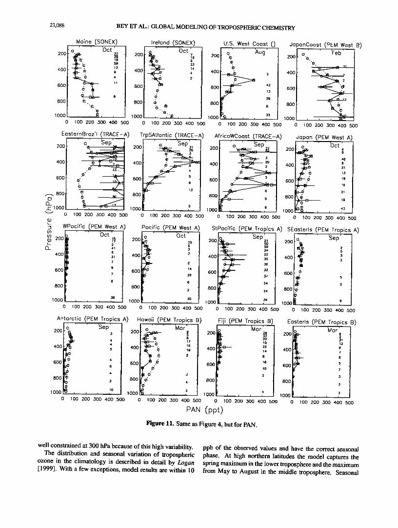
Peroxyacetylnitrate (PAN) is a reservoir species for NOx produced by oxidation of organic compounds. Observed PAN concentrations are high over the continental regions (especially where influenced by biomass burning or fossil fuel emissions) and low in regions remote from direct NO• sources. The model captures similar trends. Simulated concentrations at northern midlatitudes are consistent with observed values although the model overestimates PAN concentrations over Japan in October, a problem previously noted by Wang et al. [1998b]. Simulated PAN concentra- tions for the TRACE-A region, which was heavily impacted by biomass burning, are high but still underestimate obser- vations. Such underestimate was previously noted for ethane and may reflect insufficient NMHC emission from biomass burning in the model.

Nitric acid (HNO3) is produced in the atmosphere by reaction of NO2 with OH and by hydrolysis of N205 in aerosols. Major sinks are dry and wet deposition. Compari- son of model results with observed HNO3 concentrations is shown in Figure 12. The model typically overestimates the observations by a factor of 2-3. This problem is common to most current global 3-D models of tropospheric chemistry [Wang et al., 1998b; Hauglustaine et al., 1998; Mickley et al., 1999; Lawrence et al., 1999]. The partitioning of HNO3 into aerosols might provide an explanation since the model does not differentiate between gaseous and aerosol nitrate. There is also strong evidence that the model underestimates precipitation scavenging in the upper troposphere, as shown by Liu et al. [2001] in a simulation of 21øPb and 7Be tracers. Lawrence and Crutzen [ 1998] suggested that cirrus precipitation could lead to a considerable scavenging of HNO3 from the upper troposphere. This process is not represented in our model. (They also suggested that cirrus precipitation would scavenge H202; however, that seems

BEY ET AL.: GLOBAL MODELING OF TROPOSPHERIC CHEMISTRY 23,087

dubious since H202 is only weakly partitioned into the cirrus ice phase [Mari et al., 2000].)

3.5. Ozone

Evaluation of simulated ozone concentrations uses the

multiyear climatology of ozonesonde data presented by Logan [1999] as well as 1994 ozonesonde measurements.

Figure 13 compares simulated and observed seasonal vari- ations of ozone concentrations at 300, 500, and 800 hPa.

Where available, 1994 seasonal variations are also reported. The 1994 observations are usually within 20 ppb of the climatology, with the exception of high latitudes at 300 hPa where small shifts in tropopause height can introduce considerable variability in ozone; model evaluation is not

Maine (SONEX) Ireland (SONEX) U.S. West Coast (CITE 2) JapanCoast (PEM West B)

•oor • •oo / 400 m_.•,,/•m ''24 ' 400 [ ,,•..•._ 223 I 400 '•' 2 600 ;/• 7 • •. 600 600

800 'e e • 800 000 __• ,"e','•-e • ' - ........... •e.._ 119 I [ • ß 11 1 1000 -e ..... "- 1000 • e ........... "

0 40 80 120 160 200 0 40 80 120 160 200 0 40 80 120 160 200 0 40 80 120 160 200

EasternBrazil (TRACE-A) TrpSAtlontic (TRACE-A) AfricoWCoost (TRACE-A) Japan (PEM West A)

ß • 7 ,½ ' • ß 51

[ lO 800 4 800 ooo• , •---:-'-': .... 1 •ooo• .... , ooo• .... 'e t • 1 1000 e- _ _

0 40 80 120 160 200 0 40 80 120 160 200 0 40 80 120 160 200 0 40 80 120 160 200

WPocific (PEM West A) Pacific (PEM West A) StPoc•f•c (PEM Tropics A) SEosterls (PEM Tropics A)

; [i :, t ,, 2OO 2oo ½.- ego 2o0 r • ½• 400 •5 • ½ 9• •2

' ' 80

I ,, , ,, •ooo• •ooo'• •ooo• , , , '• 1 ,c

o 4o so 12OlSO2OO o 4o •o 12o 16o 2oo o •o so •2OlSO2OO o 4o so 1•o•o2oo

Antarctic (PEM Tropics A) ' ' ' ' r• ep 'Ma

200 • 200 •--" 7

400 21 400

22 600 600

15

800 16 800

1000 i • , 1000F• , , ,

0

Hawaii (PEM Tropics B)

106 9O 88 97

241

55

20

19

26

105

29

I

40 80 120 160 200 0 40 80 120 160 200

2OO

40O

6OO

8OO

1 ooo •

o

NO (ppt)

Fiji (PEM Tropics B)

542 572 357 298

384

268

144

247

170

87

98

236 i , I , i

40 80 120 160 200

EasterIs (PEM Tropics B)

2OO

4O0

6O0

8O0

000

0

E).• =•F':' 99 166

/, 182 "' 205

• 113 .

• 243 6 143

110

115

176 I I i I

40 80 120 160 2(

Figure 10. Same as Figure 4, but for NO.

23,088 BEY ET AL.: GLOBAL MODELING OF TROPOSPHERIC CHEMISTRY

Moine (SONEX) Irelond (SONEX) U.S. West Coost () JoponCoost (PEM West B)

t ' •, ] 200 200 •oo • •oot..• ::1•oo• ••_• 800 BOO BOO

•ooo ' ' ½' , • •' •oo• •oo' , , , 0 100 200 500 400 500 0 100 200 500 400 500 0 100 200 500 400 500 0 100 200 300 400 500

Eos(ernBroz[I (TRACE-A) TrpSAtlont[c (TRACE-A) Afr[coWCoost (TRACE-A) Jepon (PEM West A)

•oo[ • ,e•. • ,• ,• ,e•; • •oo[ •.- ,e•,, J •.• e½ T • • • 400 • • 2 •0o

•,oo • . ,oo.,• = •. ,oo• ::• •ooo• * ,• •,oo • 0 100 200 500 400 500 0 100 200 500 400 500 0 100 200 500 400 500 0 100 200 •00 400 500 L p • W ocific (PEM Wes(A) Poc[fic (PEM Wes(A) StPocific (PEM Tropics A) SEos(erl (PEM Tropics A) s

200 20 • • 200 Sep•g 200 o

, .oo : ,. ,, ' 2• 600 •7 600

6 24 2

800 [ • 801 2 •00 24 •00 1000 •6 100( •o 300 34 •00 '• , , 1 1 ,

0 100 200 300 400 500 0 100 200 300 400 500 0 100 200 300 400 500 0 100 200 300 400 500

Howoii (PEM Tropics ) Fiji (PEM Tropics B) Eosterls (PEM Tropics B)

•oo• •oo• • • •oo ' 17

.oo •oo•• • t ,oo •oo ,: 800 ]00

lOOO '- 1:oo,• •:oo• , , , • 1 •:oo• 0 100 200 300 400 500 0 100 200 300 400 500 0 100 200 300 400 500 0 100 200 300 400 500

PAN (ppt)

Figure 11. Same as Figure 4, but for PAN.

well constrained at 300 hPa because of this high variability. The distribution and seasonal variation of tropospheric

ozone in the climatology is described in detail by Logan [ 1999]. With a few exceptions, model results are within 10

ppb of the observed values and have the correct seasonal phase. At high northern latitudes the model captures the spring maximum in the lower troposphere and the maximum from May to August in the middle troposphere. Seasonal

BEY ET AL.: GLOBAL MODELING OF TROPOSPHERIC CHEMISTRY 23,089

variations at northern midlatitudes are relatively well repre- sented. However, the model tends to underestimate slightly the amplitude of the seasonal variation in the extratropics (Hohenpeissenberg and Saporro for example), a problem which we ascribe tentatively to insufficient seasonal vail-

ation of cross-tropopause transport (less than that shown by Wang et al. [1998a]). Elevated concentrations at 800 hPa at Boulder in summer are likely due to pollution from Denver, which we do not capture well in the model. Good simulation is usually achieved in the tropics and subtropics

Mc•ir,e (SONEX) Irelond (SONEX) U.S. West Coost (CITE 2) Ja,onCoost (PEM West B)

' • 'o•t' t [ ' 'o•t' t .... I .... 200 -al•--- ..o ..... '•45--'1 200I __•• .o ...... 27•-'1 200 e..o Aug 200 e 400 s 400 400 'e 400

aoo • .... 1 søøt •- I 8oo[• • • ,o ] 8oo • 1000/• ,•-e, , , / 1000 • ,R , ,

0 200 400 600 800 1000 0 200 400 600 800 000 0 200 400 600 800 1000 0 200 400 600 800 1000

Easterngrozil (TRACE-A) TrpSAtlontic (TRACE-A) AfricoWCoost (TRACE-A) Jopon (PEM West A) • 'o ' •ep' t [ "'•' bct' 2o0 % Sep •1 200 • Se• • 200 [• • f•5 I 200• • •- ß

400 • ,2 400 • • 4oo• • s 1 4oo•

& 16 5

800 • 4o 800 800 • 1000• •000 "'• • 800[ 1000/ ,•--, .... h'" , / 10001• 0 200 400 600 800 1000 0 200 400 600 800 1000 0 200 400 600 800 1000 0 200 400 600 800 1000

WPo•ific •PE• W•st A) •oci•ic (,PEM, We•t A) StPoc[f[c (PEM Tropics A) SEosterls (PEM Tropics A) ••ook o•, ] •oo [ •.• o• ] •ook,..o •e• t •ook

• 23 4

•oo• • I •oo• • I •oo • •oo

•oo• , ] •oo• • ,• t •oo•• ,, • •oo•; •oo• • ] •oor • • •oo •oo ooo• .... • ,ooom .... • •ooo• ..... I •ooo• ......

0 200 400 600 800 1000 0 200 400 600 800 1000 0 200 400 600 800 1000 0 200 400 600 800 1000

Antorctic (PEM Tropics A) Howoil (PEM Tropics B) Fij• (PEM Tropics B) Eosterls (PEM Tropics B) ' ' g•p' t [ '• ' 'Mor' t t•' ' 'Mo•' t t •' ' 'M•'

•oo .• ............. • •oo[½, •• •oo• •,• ,oo..

600 • 600 • • • • 2• • • •

8o0 8o0 • , 800• ,2 ] 800[• •ooo, , , , ; t lOOO •½• lOOO• •ooo•

0 200 400 600 800 1000 0 200 400 600 800 1000 0 200 400 600 800 1000 0 200 400 600 800 1000

HNO; (ppt) Figure 12. Same as Figure 4, but for HNO3.

23,090 BEY ET AL.: GLOBAL MODELING OF TROPOSPHERIC CHEMISTRY

Resolute (74 N, 95 W) - 800mbor Resolute (74 N, 95 W) - 500mbor Res(•lute (74 N, 95 W) - 50Orebar

,oo ........ ,oo i i i 1 200 ' ß I .....

80 80 I • 150 • 60 60

o 40 40 ' ' - -

j F M A M J J A $ 0 N D J F M A M J J A $ 0 N D J F bl A bl J J A $ 0 N D

Edmonton (55 N, 114 W) - 800mbar Edmonton (55 N, 114 W) - 500mbar Edmonton (53 N, 114 W) - 50Orebar

J F M A M J J A S 0 N D J F M A M J J A $ 0 N D J F M A M J J A S 0 N D

Hohenpe[ssenberg (47 N, 11 E) - 800mbar Hohenpe[ssenberg (47 N, 11 E) - 500mbar Hohenpeissenberg (47 N, 11 E) - 500mbar 100[ ........ 100• ............. 200 I 150

• 100 o 40 40 '

0

J F M A M J J A S 0 N D J F M A M J J A S 0 N D J F M A M J J A $ 0 N D

Sapporo (45 N, 141 E) - BOOmbar Sapporo (45 N, 141 E) - 50Orebar Sapporo (45 N, 141 E) - 50Orebar ,oo ,oo ............ f ..... , 80 80

• - • •ø I • •o •o

o 40 40

2• 2• 50 • • 0 •

J F M A M J J A S 0 N D J F M A M J J A S 0 N D J F M A M J J A S 0 N D

Boulder (40 N, 105 W) - 80Orebar Boulder (40 N, 105 W) - 50Orebar Boulder (40 N, 105 W) - 500mbor ,oo[ ,oo[• ............ .•oo ............ 80 80

• O0 o 40 40

2• 20 50 , , , , 0 0

J F M A M J J A S 0 N D J F M A M J J A S 0 N D J F M A M J J A $ 0 N D

Kogoshimo (32 N, 131 E) - 800mbor Kogoshimo (32 N, 151 E) - 500mbor Kagoshimo (32 N, 131 E) - 50Orebar

,oo ,oo ............ ,oo f ............ 80 80 / \

• 100• o 40 40 .-e ....

0 .... i • • i i • i 0 i i i • , , • J F M A M J J A • O N D J F M A M J J A S O N D J F M A M J J A S 0 N D

Figure 13. Comparison of observed and simulated monthly mean concentrations of ozone at 800, 500, and 300 hPa. Observations (open triangles and solid lines) are from the ozonesonde climatology of Logan [ 1999]; vertical bars are standard deviations corresponding to interannual variability. Long-dashed lines are the observed values for 1994 (there are no observations in 1994 at Samoa and Natal). Model values (open circles and dashed lines) are for 1994.

BEY ET AL.: GLOBAL MODELING OF TROPOSPHERIC CHEMISTRY 23,091

to within the constraints offered by the observations. The maximum due to biomass burning emissions that the model observed minima in eastern Asia (Kagoshima and Naha) captures well. The longitudinal gradient observed in the due to the summer monsoon are captured by the model. southern tropics between Natal and Samoa is also well The spring maximum and summer minimum observed in the captured. northern subtropics (Hilo, for example) are well represented Table 5 gives the global budget of tropospheric ozone by the model throughout the troposphere. Observations in the model. The global photochemical production and in the southern tropics (Natal) show a large austral spring destruction rates of ozone are 4900 Tg yr -t and 4300 Tg

,00 --

8O

• $0

o

2O

Naha (26 N, 127 E) - 80Orebar Nahe (26 N, 127 2) - 50Orebar 100 - 200

80 150

0-- '-©'. ./ • •--@- • 60 --. 100 40

20 50

0 0

J F M A M J J A $ 0 N D J F M A M J J A S 0 N D

Naha (26 N, 127 E) - 300mbar

J F M A M J J A $ 0 N D

100

80

60

40

20

Hilo (20 N, 155 W) - 800mbar

d F M A M J J A S 0 N D

Hilo (20 N, 155 W) - 50Orebar 100 200

80 150

' '-- • • ' 100 40

20 50

J .• M A M J J A S 0 N D

Hilo (20 N, 1.55 W) - 300mbor

J F M A M J J A S 0 N D

Natal (6 S, 35 W) - 800mbar Natal (6 S, 35 W) - 50Orebar lOO lOO : 2OO

80 80 150

60 60 100

40 4o

5o 20 20

o o o

j F M A M J J A S 0 N D J F M A M J J A $ 0 N D

Natal (6 S, 35 W) - 300mbar

J F M A M J J A $ 0 N D

Samoa (14 S, 170 W) - 80Orebar Samoa (14 S, 170 W) - 500mbar

lOO lOO• 80 80

60 60 •'- . . _• •o 4o .e ..... e.

20 20

,

J F M A M J J A S 0 N D J F M A M J J A $ 0 N D

200

150

1 O0

50

0

Samoa (14 S, 170 W) - 30Orebar

J F M A M J J A S 0 N D

Lauder (45 S, 169 E) - BOOmbar Lauder (45 S, 169 E) - 500mbor Lauder (45 S, 169 E) - 30Orebar

100 100•1 200 ............. 80 80 150

60 60 •oo

20 50

0 , 0 , , A, , , , • , • A ,•, • • , , • , i , , • ,

J F bl A M J J A S 0 N D O F M A M J J A S 0 N D d F M a M J O A S 0 n D

100

BO

,, 60

o 40 o

20

Syowa (69 S, 39 E) - 80Orebar Syowo (69 S, 39 E) - 500mbor 1 O0 .........

80

6O

'' 't.a-' -(• .... 0'• 40 .. ._ _o .• 0 , , , • , , • i , , • , _ , , • • , , , , , , ,

d F M A M d d A S 0 N D d F M A M d d A $ 0 N O

Syowa (69 S, 39 E) - 30Orebar 200 ....... "' ....

150

1 oo 50

o , , , • , , . , •... • , , ,

d F M A bt J d A S 0 N D

Figure 13. (continued)

23,092 BEY ET AL.: GLOBAL MODELING OF TROPOSPHERIC CHEMISTRY

Table 5. Global Budget for Tropospheric Ozone in the GEOS-CHEM Model

Global Northern Hemisphere Southern Hemisphere

Sources, Tg Oa yr- • Chemical production 4900 3100 1800 Stratospheric influx 470 280 190 Total 5370 3380 1990

Sinks, Tg Oa yr- • Chemical loss 4300 2600 1700

Deposition 1070 740 330 Total 5370 3340 2030

Burden, Tg Oa 315 175 140

The budget is for the extended odd oxygen family defined as Oa + NO2 +2 x NO3 + PAN + PPN + MPAN + HNO4 + HNO3 + 3 x N9. O5 and applies to the column up to the model tropopause. Values are annual means for 1994.

yr -•, respectively, with a stratospheric input of 470 Tg yr -•. Previous global 3-D models indicate photochemical production ranging from 3314 to 4550 Tg yr -• and photo- chemical loss ranging from 2511 to 4065 Tg yr -• [WMO, 1998; Lelieveld and Dentener, 2000]. Stratospheric inputs in these models vary from 390 to 768 Tg yr- 1 [WMO, 1998]. Our calculated values for the photochemical terms are at the high end of previous models. They are in particular higher than in our previous global 3-D models at Harvard; Mickley et al. [ 1999] and Wang et al. [ 1998b] report production rates of 4330 and 4100 Tg yr -• and loss rates of 3960 and 3680 Tg yr-•, respectively. The difference appears to reflect the stronger UV actinic fluxes in the present model, as discussed previously.

4. Conclusion

This paper provided a first description of GEOS-CHEM, a global 3-D model of tropospheric chemistry driven by GEOS assimilated meteorological fields from the NASA Data Assimilation Office (DAO). A 1-year simulation is presented for 1994, and results are evaluated with obser- vations both for 1994 and for other years. We show that the model is capable of representing the general features of the global distributions of tropospheric ozone and related species although there are some significant discrepancies.

Global chemical production and loss rates of tropospheric ozone, as well as global OH concentrations, are at the high end of values previously reported in global 3-D models including earlier generations of our 3-D model at Harvard. This difference appears largely due to our suppression of an UV-absorbing background aerosol (with an optical depth of 0.1 at 310 nm) that was present in the earlier models. Although organic aerosols in the troposphere are expected to absorb UV radiation, there are no observations available to usefully constrain the corresponding optical depth at the wavelengths of interest. The present model can accommo- date the observed methylchloroform lifetime and H202 con- centrations (which provide standard tests of photochemical activity for global models) within the constrains provided by these observations. However, that does not exclude model OH for possibly being too high by •20%.

The model systematically underestimates observed CO concentrations by 10-30 ppb, which could reflect a problem with current source inventories as well as an overestimate

of OH. Simulation of ethane indicates an underestimate of

sources. The large underestimate of acetone concentrations over the South Pacific suggests a large oceanic source. Simulated concentrations of NO and PAN are generally within a factor of 2 of observed values (often much bet- ter) and show the correct vertical structure. The model overestimates HNO3 concentrations by factors of 2-3 in the remote troposphere, a problem which we attribute in part to insufficient scavenging.

The model reproduces well the global distribution of tropospheric ozone concentrations as determined from ozonesonde observations. It simulates usually to within 10 ppb the 1994 observations as well as the multiyear climatology (which are similar except near the tropopause). it captures the observed seasonal phases and amplitudes in different regions of the troposphere. There is a slight underestimate in the amplitude of the seasonal variation in the extratropical Northern Hemisphere which we attribute to insufficient seasonal variation in the parameterized cross- tropopause ozone flux.

In a companion paper [Be), et al., this issue], we use the GEOS-CHEM model to examine the Asian outflow of

ozone, CO, and NO u species over the western Pacific by simulation of observations from the PEM-West B aircraft

mission in February-March 1994.

Acknowledgments. This research was supported by the NASA Atmospheric Chemistry Modeling and Analysis Program (ACMAP) and by the NASA Earth Observing System (EOS). We wish to thank Clarissa Spivakovsky for very helpful discussions. We are grateful to Andrew Fusco for processing isoprene observa- tions.

References

Adams, P.J., J.H. Seinfeld, D. Koch, L.J. Mickley, and D.J. Jacob, General circulation model assessment of direct radiative forcing by the sulfate-nitrate-ammonium-water inorganic aerosol sys- tem, J. Geophys. Res., 106, 1097-1111,2001.

Allen, D.J., R.B. Rood, A.M. Thompson, and R.D. Hidson, Three- dimensional 9'9'9'Rn calculations using assimilated data and a

BEY ET AL.: GLOBAL MODELING OF TROPOSPHERIC CHEMISTRY 23,093

convective mixing algorithm, J. Geophys. Res., 101, 6871-6881, 1996a.

Allen, D.J., et al., Transport induced interannual variability of carbon monoxide using a chemistry and transport model, J. Geophys. Res., 101, 28,655-28,670, 1996b.

Andronache, C., W.L. Chameides, M.O. Rodgers, J. Martinez, P. Zimmerman, and J. Greenberg, Vertical distribution of isoprene in the lower boundary layer of the rural and urban southern United States, J. Geophys. Res., 99, 16,989-16,999, 1994.

Atkinson, R., Gas-phase tropospheric chemistry of volatile organic compounds, 1, Alkanes and alkenes, J. Phys. Chem. Reft Data, 26, 215-290, 1997.

Benkovitz, C.M., M.T Schultz, J. Pacyna, L. Tarrason, J. Dignon, E.C. Voldrier, P.A. Spiro, J.A. Logan, and T.E. Graedel, Global gridded inventories for anthropogenic emissions of sulfur and nitrogen, J. Geophys. Res., 101, 29,239-29,253, 1996.

Bey, I., D.J. Jacob, J.A. Logan, and B. Yantosca, Asian chemical outflow to the Pacific in spring: Origins, pathways, and budgets, J. Geophys. Res., this issue.

Brasscur, G.P., D.A. Hauglustaine, S. Walters, P.J. Rasch, J.E Mtiller, C. Granier, and X.X. Tie, MOZART, A global chemical transport model for ozone and related chemical tracers, 1, Model description, J. Geophys. Res., 103, 28,265-28,289, 1998.

Brown, S.S., R.K. Talukdar, and A.R. Ravishankara, Rate constant for the reaction OH+NO2+M • HNOa+M under atmospheric conditions, Chem. Phys. Lett., 299, 277-284, 1999a.

Brown, S.S., R.K. Talukdar, and A.R. Ravishankara, Reconsider- ation of the rate constants for the reaction of hydroxyl radicals with nitric acid vapor, J. Phys. Chem., 103, 3031-3037, 1999b.

Chen, X.H., D. Hulbert, P.B. Shepson, Measurement of the organic nitrate yield from OH reaction with isoprene, J. Geophys. Res., 103, 25,563-25,568, 1998.

Chin, M., D.J. Jacob, G.M. Gardner, M.S. Foreman-Fowler, P.A. Spiro, and D.L. Savoie, A global three-dimensional model of tropospheric sulfate, J. Geophys. Res., 101, 18,667-18,690, 1996.

Collins, W.J., D.S. Stevenson, C.E. Johnson, and R.G. Der- went, Tropospheric ozone in a global-scale three-dimensional lagrangian model and its response to N O•: emission controls, J. Atmos. Chem., 26, 223-274, 1997.

DeMore, W.B., S.P. Sander, D.M. Golden, R.F. Hampson, M.J Kurylo, C. J. Howard, A. R. Ravishankara, C.E. Kolb, and M.J. Molina, Chemical kinetics and photochemical data for use in stratospheric modeling, JPL Publ., 97-4, 1997.

European Monitoring and Evaluation Programme (EMEP), Trans- boundary air pollution in Europe, part 1, Emissions, dispersion and trends of acidifying and eutrophying agents, EMEP/MSC-W Rep. 1/97, Norw. Meteorol. Inst., Oslo, Norway, 1997.

Emmons, L.K., D.A. Hauglustaine, J.F. Mtiller, M.A. Carroll, G.P. Brasscur, D. Brunner, J. Staehelin, V. Thouret, and A. Marerico, Data composites of airborne observations of tropospheric ozone and its precursors, J. Geophys. Res., 105, 20497-20538, 2000.

Environmental Protection Agency (EPA), National air pollutant emission trends, 1990-1996, Rep. EPA-454/R-97-011, Research Triangle Park, N.C., 1997.

Flatoy, F., O. Hov, and H. Schlager, Chemical forecasts used for measurement flight planning during POLINAT 2, Geophys. Res. Lett., 27, 951-954, 2000.

Granier, C., G. Petton, J.-E Mtiller, and G. Brasscur, The impact of natural and anthropogenic hydrocarbons on the tropospheric budget of carbon monoxide, Atmos. Environ., 34, 5255-5270, 2000.

Guenther, A., et alo, A global model of natural volatile organic compound emissions, J. Geophys. Res., 100, 8873-8892, 1995.

Guenther, A., et al., Isoprene fluxes measured by enclosure, relaxed eddy accumulation, surface layer gradient, mixed layer gradient, and mixed layer mass balance techniques, J. Geophys. Res., 101, 18,555-18,567, 1996.

Hansen, J., G. Russell, D. Rind, P. Stone, A. Lacis, S. Lebedeff, R. Ruedy, and L. Travis, Efficient three-dimensional models for

climate studies: Models I and II, Mon. Weather Rev., 3, 609-662, 1983.

Hauglustaine, D.A., G.P. Brasseur, S. Walters, P.J. Rasch, J.F. Mtiller, L.K. Emmons, and M.A. Carroll, MOZART: A global chemical transport model for ozone and related chemical tracers, 2, Model results and evaluation, J. Geophys. Res., 103, 28,291- 28,335, 1998.

Helmig, D., et al., Vertical profiling and determination of landscape fluxes of biogenic nonmethanes hydrocarbons within the plane- tary boundary layer in the Peruvian Amazon, J. Geophys. Res., 103, 25,519-25,532, 1998.

Hoell, J.M., D.D. Davis, S.C. Liu, R.E. Newell, M. Shipham, H. Akimoto, R.J. McNeal, R.J. Bendura, and J.W. Drewry, Pacific Exploratory Mission West-A (PEM West-A): September- October 1991, J. Geophys. Res., 101, 1641-1653, 1996.

Hoell, J.M., et al., Pacific Exploratory Mission-West Phase B: February-March 1994, J. Geophys. Res., 102, 28,223-28,240, 1997.

Hoell, J.M., D.D. Davis, D.J. Jacob, M.O. Rodgers, R.E. Newell, H.E. Fuelberg, R.J. McNeal, J.L. Raper, and R.J. Bendura, The Pacific Exploratory Mission in the tropical Pacific: PEM-Tror)ic.q A, August-September 1996, J. Geophys. Res., 104, 5567-5584, 1999.

Holloway, T., H. Levy II, and P. Kasibhatla, Global distribution of carbon monoxide, J. Geophys. Res., 105, 12,123-12,147, 2000.

Horowitz, L.W., and D.J. Jacob, Global impact of fossil fuel combustion on atmospheric NOx J. Geophys. Res., 104, 23,823- 23,840, 1999.

Horowitz, L.W., J. Liang, G.M. Gardner, and D.J. Jacob, Export of reactive nitrogen from North America during summertime: Sensitivity to hydrocarbon chemistry, J. Geophys. Res., 103, 13,451-13,476, 1998.

Intergovernmental Panel on Climate Change (IPCC), Radiative forcing of climate change and an evaluation of the IPCC IS92 emission scenarios, in Climate Change 1994: The Science of Climate Change, edited by J.T. Houghton et al., Cambridge Univ. Press, New York, 1995.

Intergovernmental Panel on Climate Change (IPCC), Atmospheric chemistry and greenhouse gases, in Climate Change 2001: The Scientific Basis, edited by J.T. Houghton et al., Cambridge Univ. Press, New York, 2001.

Jacob, D.J., Heterogeneous chemistry and tropospheric ozone, Atmos. Environ., 34, 2131-2159, 2000.

Jacob, D.J., et al., Evaluation and intercomparison of global atmospheric transport models using radon-222 and other short- lived tracers, J. Geophys. Res., 102, 5953-5970, 1997.

Jacob, D.J., et al., Origin of ozone and NOx in the tropical troposphere: A photochemical analysis of aircraft observations over the South Atlantic Basin, J. Geophys. Res., 101, 24,235- 24,250, 1996.

Jacobson, M.Z., and R.P. Turco, A sparse-matrix, vectorized GEAR code for atmospheric transport models, Atmos. Environ., 33, 273-284, 1994.

Kanakidou, M., et al., 3D global simulations of tropospheric CO distributions - Results of the GIM/IGAC intercomparison 1997 exercise, Chemosphere Global Change Sci., 1, 263-282, 1999.

Klinger, L.F., J. Greenberg, A. Guenther, G. Tyndall, P. Zimmer- man, M. M'Bangui, J.M. Moutsambot, and D. Kenfck, Pat- terns in volatile organic compound emissions along a savanna- rainforest gradient in central Africa, J. Geophys. Res., 103, 1443- 1454, 1998.

Lawrence, M.G., and P.J. Crutzen, The impact of cloud particle gravitational settling on soluble trace gas distributions, Tellus, 50, 263-289, 1998.

Lawrence, M.G., P.J. Crutzen, P.J. Rasch, B.E. Eaton, and N.M. Mahowald, A model for studies of tropospheric photochemistry: Description, global distributions, and evaluation, J. Geophy& Res., 104, 26,245-26,277, 1999.

Lee, M., B. G. Heikes, D.J. Jacob, G. Sachse, and B. Anderson, Hydrogen peroxide, organic hydroperoxide, and formaldehyde

23,094 BEY ET AL.: GLOBAL MODELING OF TROPOSPHERIC CHEMISTRY

as primary pollutants from biomass burning, J. Geophys. Res., 102, 1301-1309, 1997.

Levy, H., W.J. Moxim, A.A. Klonecki, and P.S. Kasibhatla, Simu- lated tropospheric NOs: Its evaluation, global distribution, and individual source contributions, J. Geophys. Res., 104, 26,279- 26,306, 1999.

Lelieveld, J., and F.J. Dentener, What controls tropospheric ozone?, J. Geophys. Res., 105, 3531-3551, 2000.

Li, Q., D.J. Jacob, I. Bey, R.M. Yantosca, Y. Zhao, Y. Kondo, and J. Notholt, Atmospheric hydrogen cyanide (HCN): Biomass burning source, ocean sink? Geophys. Res. Lett., 27, 357-360, 2000.

Liang, J., L.W. Horowitz, D.J. Jacob, Y. Wang, A.M. Fiore, J.A. Logan, G.M. Gardner, and J.W. Munger, Seasonal budgets of reactive nitrogen species and ozone over the United States, and export fluxes to the global atmosphere, d. Geophys. Res., 103, 13,435-13,450, 1998.

Lin, S.-J., and R. B. Rood, Multidimensional flux form semi-

Lagrangian transport schemes, Mort. Weather Rev., 124, 2046- 2070, 1996.

Liu, H., D.J. Jacob, I. Bey, and R.M. Yantosca, Constraints from 2•øPb and ZBe on wet deposition and transport in a global three-dimensional chemical tracer model driven by assimilated meteorological fields, d. Geophys. Res., 106, 12,109-12,128, 2001.

Logan, J.A., An analysis of ozondesonde data for the troposphere: Recommendations for testing 3-D models and development of a gridded climatology for tropospheric ozone, J. Geophys. Res., 104, 16,115-16,149, 1999.

Logan, J.A., M.J. Prather, S.C. Wofsy, and M.B. McElroy, Tropo- spheric chemistry: A global perspective, d. Geophys. Res., 86, 7210-7254, 1981.

Mari, C., D.J. Jacob, and P. Bechtold, Transport and scavenging of soluble gases in a deep convective cloud, d. Geophys. Res., 105, 22,255-22,267, 2000.

Marland, G., T.A. Boden, R. J. Andres, A. L. Brenkert, and C. A. Johnston, Global, regional, and national fossil fuel CO2 emis- sions, In Trends: A Compendium of Data on Global Change, Carbon Dioxide Inf. Anal. Cent., Oak Ridge Nat. Lab., U.S. Dep. of Energy, Oak Ridge, Tenn., 1999.

McLinden, C.A., S.C. Olsen, B. Hannegan, O. Wild, M.J. Prather, and J. Sundet, Stratosphefic ozone in 3-D models: A simple chemistry and the cross-tropopause flux, J. Geophys. Res., 105, 14,653-14,665, 2000.

Micldey, L.J., P.P. Murti, D.J. Jacob, J.A. Logan, D. Rind, and D. Koch, Radiative forcing from tropospheric ozone calculated with a unified chemistry-climate model, J. Geophys. Res., 104, 30,153-30,172, 1999.

Middleton, P., W.R. Stockwell, and W.P.L. Carter, Aggregation and analysis of volatile organic compounds emissions for regional modeling, Atmos. Environ., 24, 1107-1133, 1990.

Novelli, P.C., K.A. Masarie, and P.M. Lang., Distributions and recent changes in carbon monoxide in the lower troposphere, J. Geophys. Res., 103, 19,015-19,033, 1998.

Palmer, P.I., D.J. Jacob, K. Chance, R.V. Martin, R.J.D. Spun', T.P. Kurosu, I. Bey, R.M. Yantosca, A. Fiore, and Q. Li, Air mass factor formulation for spectroscopic measurements from satellites: Application to formaldehyde retrievals from the Global Ozone Monitoring Experiment J. Geophys. Res., 104 14,539-14,550, 2001.

Piccot, S.D., J.J. Watson, and J.W. Jones, A global inventory of volatile organic compound emissions from anthropogenic sources, J. Geophys. Res., 97, 9897-9912, 1992.

Pickering, K. E., et al., Convective transport of biomass burning emissions over Brazil during TRACE-A, J. Geophys. Res., 101, 23,993-24,012, 1996.

Prinn, R.G., R.E Weiss, B.R. Miller, J. Huang, EN. Alyea, D.M. Cunnold, P.J. Fraser, D.E. Hartley, and P.G. Simmonds,

Atmospheric trends and lifetime of CH:•CCla and global OH concentrations, Science, 269, 187-192, 1995.

Raper, J.L., M.M. Kleb, D.J. Jacob, D.D. Davis, R.E. Newell, H.E. Fuelberg, R.J. Bendura, J.M. Hoell, and R.J. McNeal, Pacific Exploratory Mission in the tropical Pacific: PEM-Tropics B, March-April 1999, d. Geophys. Res., in press, 2001.

Rasch, P.J., et al., A comparison of scavenging and deposition processes in global models: Results from the WCRP Cambridge Workshop of 1995, Tellus, 52, 1025-1056, 2000.

Reissell, A., C. Harry, S.M. Aschmann, R. Atkinson, and J. Arey, Formation of acetone from the OH radical- and Oa-initiated reactions of a series of monoterpenes, J. Geophys. Res., 104, 13,869-13,879, 1999.

Rind, D., and J. Lerner, Use of on-line tracers as a diagnostic tool in general circulation model development, 1, Horizontal and vertical transport in the troposphere, J. Geophys. Res., 10], 12,667-12,683, 1996.

Roelofs, G.J., J. Lelieveld, and R. van Doffand, A three- dimensional chemistry/general circulation model simulation of anthropogenically derived ozone in the troposphere and its radiative forcing, d. Geophys. Res., 102, 23,389-23,401, 1997.

Rudolph, L., The tropospheric distribution and budget of ethane, J. Geophys. Res., 100, 11,369-11,381, 1995.

Schneider, H.R., D.B.A. Jones, G.-Y. Shi, and M.B. McElroy, Analysis of residual mean transport in the stratosphere, 1, Model description and comparison with satellite data, J. Geophys. Res., 105, 19,991-20,011, 2000.

Schubert, S.D., R.B. Rood, and J. Pfaendtner, An assimilated data set for earth science applications, Bull. Arner. Meteorol. Soc., 74, 2,331-2,342, 1993.

Schultz, M., D.J. Jacob, J.D. Bradshaw, S.T. Sandholm, J.E. Dibb, R.W. Talbot, and H.B. Singh, Chemical NO•: budget in the upper troposphere over the tropical South Pacific, J. Geophys. Res., 105, 6,669-6,679, 2000.

Singh, H.B., et al., Latitudinal distributions of reactive nitrogen in the free troposphere over the Pacific Ocean in late winter/early spring, J. Geophys. Res., 103, 28,237-28,246, 1998.

S ingh, H.B., A.M. Thompson, and H. Schlager, SONEX airborne mission and coordinated POLINAT-2 activity: Overview and accomplishments, Geophys. Res. Lett., 26, 3053-3056, 1999.

Singh, H.B., et al., Distributed and fate of select oxygenated organic species in the troposphere and lower stratosphere over the Atlantic, J. Geophys. Res., 105, 3795-3805, 2000a.

Singh, H.B., Y. Chen, A.C. Staudt, D.J. Jacob, D.R. Blake, B.G. Heikes, and J. Snow, Dominant presence of oxygenated organic species in the remote southern Pacific troposphere, Nature, 410, 1078-1081, 2000b.

Spivakovsky, C.M., R. Yevich, J.A. Logan, S.C. Wofsy, and M.B. McElroy, Tropospheric OH in a three-dimensional chemical tracer model: An assessment based on observations of CHaCCla, J. Geophys. Res., 95, 18441-18,471, 1990.

Spivakovsky, C.M., et al., Three-dimensional climatological distri- bution of tropospheric OH: Update and evaluation, J. Geophys. Res., 105, 8931-8980, 2000. ß

Toon, O.B., and R.C. Miakelye, Subsonic aircraft - contrail and cloud effects special study (SUCCESS), Geophys. Res. Lett., 25, 1109-1112, 1998.

United Nations, 1996 energy statistics yearbook, Stat. Div., U. N. Dep. for Econ. and Soc. Inf. and Pol. Anal., New York, 1998.

Wesely, M.L., Parameterization of surface resistance to gaseous dry deposition in regional-scale numerical models, Atmos. Environ., 23, 1293-1304, 1989.

Wild, O., Q. Zhu, and M.J. Prather, Fast-J: Accurate simulation of in- and below-cloud photolysis in global chemical models, J. Atmos. Chem., 37, 245-282, 2000.

World Meteorological Organization (WMO), Scientific assessment of ozone depletion: 1998, Rep. 44, Global Ozone Obs. Syst., Geneva, Switzerland, 1998.

BEY ET AL.: GLOBAL MODELING OF TROPOSPHERIC CHEMISTRY 23,095

I. Bey, Swiss Federal Institute of Technology (EPFL), DGR- LPAS, CH-1015 Lausanne., Switzerland. (e-mail: isabelle.bey @ epfl.ch)

B. D. Field, A.M. Fiore, D. J. Jacob, Q. Li, H. Y. Liu, J. A. Logan, L. J. Mickley, R. M. Yantosca, Division of Engineering and Applied Sciences and Department of Earth and Planetary Sciences, Harvard University, 29 Oxford St., Cambridge, MA 02138. re- mail: bdf; amf; djj; qli; hyl; jal; ljm; bmy@io.harvard.edu)

M. G. Schultz, Max-Planck-Institut ffir Meteorologie, Bundesstr. 55, D-20146 Hamburg, Germany. (e-mail: martin.schultz @ dkrz. de)

(Received December 20, 2000; revise(i A?fil • 6, 201)1; ,,':•cccpied April 27, 200? .',