HAL Id: pasteur-02914599https://hal-pasteur.archives-ouvertes.fr/pasteur-02914599

Submitted on 12 Aug 2020

HAL is a multi-disciplinary open accessarchive for the deposit and dissemination of sci-entific research documents, whether they are pub-lished or not. The documents may come fromteaching and research institutions in France orabroad, or from public or private research centers.

L’archive ouverte pluridisciplinaire HAL, estdestinée au dépôt et à la diffusion de documentsscientifiques de niveau recherche, publiés ou non,émanant des établissements d’enseignement et derecherche français ou étrangers, des laboratoirespublics ou privés.

Glider soaring via reinforcement learning in the fieldGautam Reddy, Jérôme Wong Ng, Antonio Celani, Terrence Sejnowski,

Massimo Vergassola

To cite this version:Gautam Reddy, Jérôme Wong Ng, Antonio Celani, Terrence Sejnowski, Massimo Vergassola. Glidersoaring via reinforcement learning in the field. Nature, Nature Publishing Group, 2018, 562 (7726),pp.236-239. �10.1038/s41586-018-0533-0�. �pasteur-02914599�

Soaring through reinforcement learning in the field

Gautam Reddy1*, Jerome Wong Ng1*, Antonio Celani2, Terrence J. Sejnowski3,4, Massimo

Vergassola1

1Department of Physics, University of California San Diego, La Jolla, USA, 2The Abdus Salam

International Center for Theoretical Physics, I-34014 Trieste, Italy, 3The Salk Institute for Biological

Studies, La Jolla, USA and 4Division of Biological Sciences, University of California, San Diego, La

Jolla, USA.

*These authors contributed equally to this work.

Abstract 1

Soaring birds often rely on ascending thermal plumes in the atmosphere as they search for 2

prey or migrate across large distances1-4. The landscape of convective currents is rugged 3

and rapidly shifts on timescales of a few minutes as thermals constantly form, disintegrate, 4

or are transported away by the wind5-6. How soaring birds find and navigate thermals within 5

this complex landscape is unknown. Reinforcement learning7 provides an appropriate 6

framework to identify an effective navigational strategy as a sequence of decisions taken in 7

response to environmental cues. Here, we use reinforcement learning to train gliders in the 8

field to autonomously navigate atmospheric thermals. Gliders of two-meter wingspan were 9

equipped with a flight controller that enables an on-board implementation of autonomous 10

flight policies via precise control over their bank angle and pitch. A navigational strategy was 11

determined solely from the gliders' pooled experiences collected over several days in the 12

field using exploratory behavioral policies. The strategy relies on novel on-board methods to 13

accurately estimate the local vertical wind accelerations and the roll-wise torques on the 14

glider, which serve as navigational cues. We establish the validity of our learned flight policy 15

through field experiments, numerical simulations, and estimates of the noise in 16

measurements that is unavoidably present due to atmospheric turbulence. This is a novel 17

instance of learning a navigational task in the field, where learning is severely challenged by 18

a multitude of physical effects and the unpredictability of the natural environment. Our results 19

highlight the role of vertical wind accelerations and roll-wise torques as viable biological 20

mechanosensory cues for soaring birds, and provide a navigational strategy that is directly 21

applicable to the development of autonomous soaring vehicles. 22

23

Main 24

In reinforcement learning, an animal maximizes its long-term reward by taking actions in 25

response to its external environment and internal state. Learning occurs by reinforcing 26

behavior based on feedback from past experiences. Similar ideas have been used to 27

develop intelligent agents, reaching spectacular performance in strategic games like 28

backgammon8 and Go9, visual-based video game play10 and robotics11,12. In the field, 29

physical constraints fundamentally prevent learning agents from using data-intensive 30

learning algorithms and the optimization of model design needed for quicker learning, which 31

are the conditions most often faced by living organisms. 32

33

A striking example in nature is provided by thermal soaring, where the extent of atmospheric 34

convection is not consistent across days and, even under suitable conditions, the locations, 35

sizes, durations and strengths of nearby thermals are unpredictable. As a result, the 36

statistics of training samples are skewed on any particular day. At smaller spatial and 37

temporal scales, fluctuations in wind velocities are due to turbulent eddies lasting a few 38

seconds that may mask or falsely enhance a glider's estimate of its mean climb rate. 39

Further, the measurement of navigational cues using standard instrumentation may be 40

consistently biased by aerodynamic effects, which requires precise quantification. Here, we 41

demonstrate that reinforcement learning can meet the challenge of learning to effectively 42

soar in atmospheric turbulent environments. To contrast with past work, the maneuvering of 43

an autonomous helicopter in ref. 11 is a control problem that is decoupled from 44

environmental fluctuations and has little trial-to-trial variability. Past autonomous soaring 45

algorithms have largely relied on locating the centroid of a drifting Gaussian thermal13-16, 46

which is unrealistic, or have applied learning methods in highly simplified simulated 47

settings17-19. 48

49

Using the reinforcement learning framework7, we may describe the behavior of the glider as 50

an agent traversing different states (s) by taking actions (a) while receiving a local reward (r). 51

The goal is to find a behavioral policy that maximizes the “value”, i.e., the mean sum of 52

future rewards up to a specified horizon. We seek a model-free approach, which estimates 53

the value of different actions at a particular state (called the Q function) solely through the 54

agent's experiences during repeated instances of the task, thereby bypassing the modeling 55

of complex atmospheric physics and aerodynamics (see Methods). The optimal policy is 56

subsequently derived by taking actions with the highest Q value at each state, where the 57

state includes sensorimotor cues and the glider's aerodynamic state. 58

59

To identify mechanosensory cues that could guide soaring, we recently combined above 60

ideas with simulations of virtual gliders in numerically generated turbulent flow20. Two cues 61

emerged from our screening: (1) the vertical wind acceleration (az) along the glider’s path; 62

(2) the spatial gradients in the vertical wind velocity across the wings of the glider (⍵). 63

Intuitively, the two cues correspond to the gradient of the vertical wind velocity in the 64

longitudinal and lateral directions of the glider, which locally orient it towards regions of 65

higher lift. Simulations in ref. 20 further showed that the glider's bank angle is the crucial 66

aerodynamic control variable; additional variables, such as the angle of attack, or other 67

mechanosensory cues, such as temperature or vertical velocity, offer minor improvements 68

when navigating within a thermal. 69

70

To learn to soar in the field, we used a glider (of two-meter wingspan) with autonomous 71

soaring capabilities (Figures 1A-B). The glider is equipped with a flight controller, which 72

implements a feedback control system used to modulate the glider's ailerons and elevator 73

such that a desired bank angle and pitch are maintained. Relevant measurements, such as 74

the altitude, ground velocity (u), airspeed, bank angle (μ) and pitch, are made continuously 75

at 10 Hz using standard instrumentation (see Methods). At fixed time intervals, the glider 76

changes its heading by modulating its bank angle in accordance with the implemented 77

behavioral policy. 78

79

Noise and biases that affect learning in the field require the development of appropriate 80

methods to extract environmental cues from sensory devices’ measurements. We found that 81

estimating az by the derivative of the vertical ground velocity (uz), is significantly biased by 82

longitudinal motions of the glider about the pitch axis as the glider responds to an imbalance 83

of forces and moments while turning. By modeling the glider's longitudinal dynamics, we 84

obtain an unbiased estimate of the local vertical wind velocity (wz), and az as its derivative 85

(Methods). The estimation of the spatial gradients across the wings, ⍵, poses a greater 86

challenge as it involves the difference between two noisy measurements at relatively close 87

positions. The key observation we used here is that the glider rolls due to contributions from 88

vertical wind velocity gradients, the feedback control mechanism and various aerodynamic 89

effects. The resulting roll-wise torque can be estimated from the small deviations of the true 90

bank angle from the desired one, and a novel dynamical model allows us to separate the ⍵ 91

contribution due to velocity gradients from the other effects (Methods). A sample trace of the 92

resulting unbiased estimate of ⍵ is shown in Figure 1C-D, together with traces of the vertical 93

wind velocity, wz, μ and unbiased estimates of az. 94

95

Equipped with a proper procedure for estimating environmental cues, we next addressed the 96

specifics of learning in the field. First, to constrain our state space, we discretized the range 97

of values of az and ⍵ into three states each, positive high (+), neutral (0) and negative high (-98

). Second, we found that learning is accelerated by choosing az attained at the subsequent 99

time step as the reward signal. The choice of az (rather than wz) is an instance of reward 100

shaping that is justified in the Supplementary Information, where we show that using az as a 101

reward still leads to a policy that optimizes the long-term gain in height. This property is a 102

special case of our general result that a particular reward function or its time derivatives (of 103

any order) yield the same optimal policy (Supplementary Information). Choosing wz as the 104

reward fails to drive learning in the soaring problem, possibly because the velocities (and 105

thus the rewards) are correlated across states and their temporal statistics strongly deviates 106

from the Markovianity assumption in reinforcement learning methods7. Indeed, velocity 107

fluctuations in turbulent flow are long-correlated, i.e. their correlation timescale is determined 108

by the largest timescale of the flow (see for instance Fig. 9 of ref. 21), which is of the order of 109

minutes in the atmosphere. Conversely, the correlation timescale of accelerations is 110

controlled by the smallest timescale21-23 (the dissipation timescale in Fig. 7 of ref. 21). This is 111

estimated to be only a fraction of a second, which is much smaller than the time interval 112

between successive actions. Note that the previous experimental observations can be 113

rationalized by the combination of the power-law spectrum of turbulent velocity fluctuations 114

in the atmosphere and the extra factor of frequency squared in the spectrum of acceleration 115

vs velocity fluctuations23. Finally, the glider's experiences, represented as state-action-state-116

reward quadruplets, (st,at,st+1,rt), were cumulatively collected (over 15 days) into a set E 117

using explorative behavioral policies. Learning is monitored by bootstrapping the standard 118

deviation of the Q values from E (Figure 2A), calculated using value iteration methods 119

(Methods). 120

121

The navigational strategy derived at the end of the training period is presented in Figure 2B, 122

which shows the actions deemed optimal for the 45 possible states. Remarkably, the rows 123

corresponding to ⍵ = 0 resemble the so-called Reichmann rules24 -- a set of simple heuristics 124

for soaring, which suggest a decrease/increase in bank angle when the climb rate 125

increases/decreases. Our strategy also gives a prescription for bank: for instance, when az 126

and ⍵ are both positive (top row in Figure 2B) i.e., in a situation when better lift is available 127

diagonal to the glider's heading, it is advantageous to bank not to the extreme but rather 128

maintain an intermediate value between -30o and -15o. Importantly, the learned 129

leftward/rightward bias in bank angle on encountering a positive/negative torque validates 130

our estimation procedure for ⍵. 131

132

In Figure 3A, we show a sample trajectory of the glider implementing the navigational 133

strategy in the field to remain aloft for ~12 minutes while spiraling to the height of low-lying 134

clouds (see also Extended Data Figure 1). On a day with strong atmospheric convection, the 135

time spent aloft is limited only by visibility and the receiver’s range as the glider soars higher 136

or is constantly pushed away by the wind. A significant improvement in median climb rate of 137

0.35 m/s was measured in the field by performing repeated 3-minute trials over five days 138

(Figure 3B, Mann-Whitney U = 429, ncontrol = 37, nstrategy = 49, p < 10-4 two-sided). Notably, this 139

value reflects a general improvement in performance averaged across widely variable 140

conditions without controlling for the availability of nearby thermals. 141

142

To examine possible advantages of larger gliders due to improved torque estimation, we 143

further analyzed soaring performance for different wingspans (I). While the naive expectation 144

is that the signal-to-noise ratio (SNR) in the estimation of ⍵ scales linearly with l, we show 145

that the effects of atmospheric turbulence lead to a much weaker l1/6 scaling (Methods). 146

Since testing our prediction would require a series of gliders with different wingspans, we 147

turned to numerical simulations of the convective boundary layer, adapted to reflect our 148

experimental setup (Methods). Results shown in Figure 3C-D are consistent with the 149

predicted scaling. Intuitively, the weak 1/6th exponent arises because the improvement in 150

gradient estimation is offset by the larger turbulent eddies, which only have a sweeping 151

effect for smaller wingspans, and contribute to velocity differences across the wings as l 152

increases. Our calculation yields an estimate of the SNR ~ 4 for typical experimental values; 153

similar arguments for az yield an SNR ~ 7. Experimental results, together with simulations 154

and SNR estimates, establish az and ⍵ as robust navigational cues for thermal soaring. 155

156

The real-world intricacies of soaring impose severe constraints on the complexity of the 157

underlying models, reflecting a fundamental trade-off between learning speed and 158

performance. Notably, the choice of a proper reward signal was crucial to make learning 159

feasible with the limited samples available. Though reward shaping has received some 160

attention in the machine learning community25, its relevance for behaving animals remains 161

poorly understood. We remark that our navigational strategy constitutes a set of general 162

reactive rules with no learning performed during a particular thermal encounter. A soaring 163

bird may use a model-based approach of constantly updating its estimate of nearby 164

thermals’ location based on recent experience and visual cues. Still, the importance of 165

vertical wind accelerations and torques for our policy suggests that they are likely useful for 166

any other strategy; our methods to estimate them in a glider suggest that they should be 167

accessible to birds as well. The hypothesis that birds utilize those mechanical cues while 168

soaring can be tested in experiments. 169

170

Finally, we note that single-thermal soaring is just one face of a multifaceted question: how 171

should a migrating bird or a cross-country glider fly among thermals over hundreds of 172

kilometers for a quick, yet risk-averse, journey26-28? This calls for the development of 173

effective methods for identifying areas of strong updraft based on mechanical and visual 174

cues. Such methods, coupled with our current work, pave the way towards a better 175

understanding of how birds migrate and the development of autonomous vehicles that can 176

extensively fly with minimal energy cost. 177

178

Main Figure Legends 179

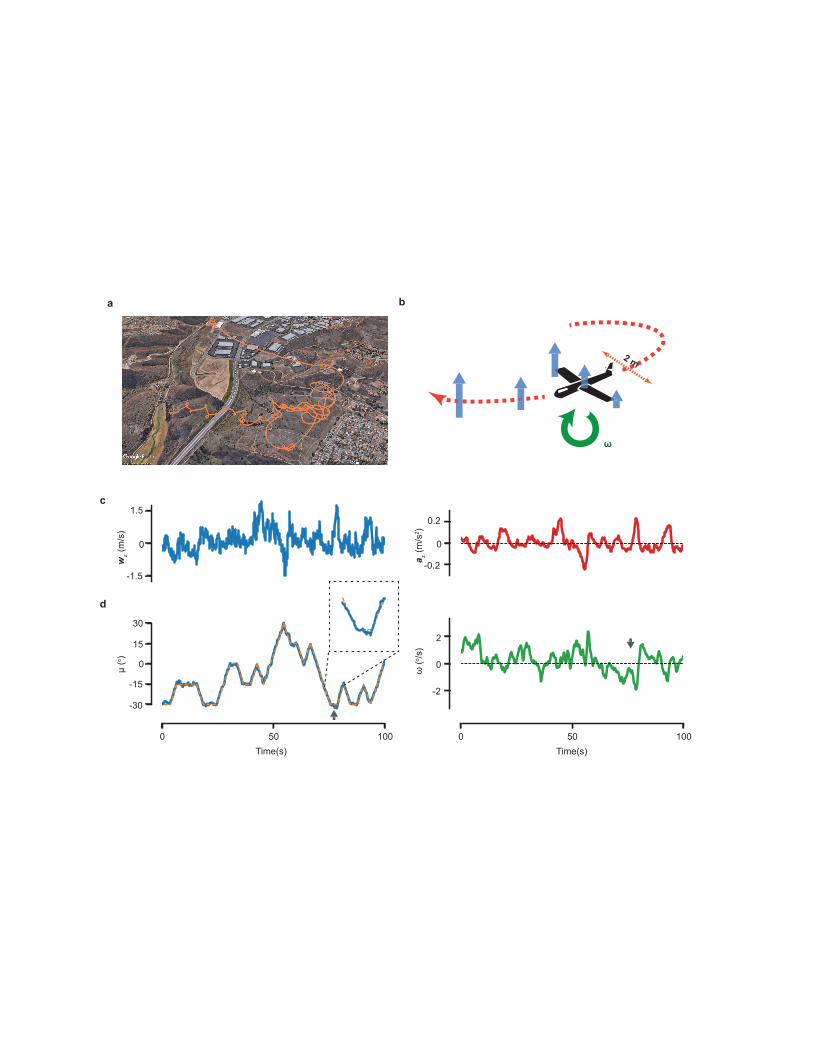
Figure 1: Soaring in the field using turbulent navigational cues. (a) A trajectory of our 180

glider soaring in Poway, California. (b) A cartoon of the glider showing the available 181

navigational cues -- gradients in vertical wind velocities along the trajectory and across its 182

wings, which generate a vertical wind acceleration az and a roll-wise torque ω respectively. 183

(c) A sample trace of the estimated vertical wind velocity wz and az obtained in the field. (d) 184

The measured bank angle μ and the estimated ω during the same trial as in panel (c). The ω 185

(solid, green) is estimated from the small deviations of the measured bank angle (solid, blue) 186

from the expected bank angle (dashed, orange) after accounting for other effects (Methods). 187

188

Figure 2: Convergence of the learning algorithm and the learned thermalling strategy. 189

(a) The convergence of Q values during learning as measured by the standard deviation of 190

the mean Q value vs training time in the field, obtained by bootstrapping from the 191

experiences accumulated up to that point. (b) The final learned policy. Each symbol 192

corresponds to the best action (increasing/decreasing the bank angle μ by 15o or maintain 193

the same μ, as shown in the legend) to be taken when the glider observes a particular (az,ω) 194

pair and is banked at μ. Combined symbols depict pairs of actions that are equally 195

rewarding. Note that a positive ω corresponds to a higher vertical wind velocity on the left 196

(right) wing of the glider and a positive (negative) μ corresponds to turning right (left) w.r.t the 197

glider’s heading. 198

199

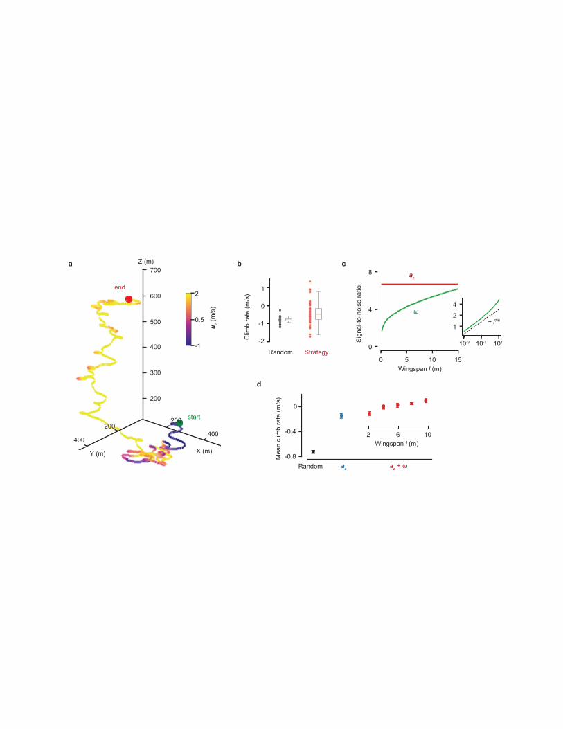
Figure 3: Performance of the learned strategy and its dependence on the wingspan. 200

(a) A 12-minute-long trajectory of the glider executing the learned thermalling strategy in the 201

field, colored by the vertical ground velocity uz at each instant. (b) Experimentally measured 202

climb rate of a control random policy (black dots) is compared against the learned strategy 203

(red dots) over repeated 3-minute trials in the field. Each dot represents the average climb 204

rate in a single trial. A few outliers are not shown to restrict the range of the axis. (c) 205

Estimated signal-to-noise ratio (SNR) in ω and az estimation vs wingspan (l) shown in green 206

and red respectively. The SNR for ω estimation is plotted in log-log scale (inset) to highlight 207

the weak l1/6 scaling. (d) The mean climb rate for the learned strategy is compared for 208

different wingspans (red dots) in simulations of a glider soaring in the convective boundary 209

layer. For comparison we show the mean climb rates for a random policy and a strategy that 210

uses az only (Methods). Error bars represent s.e.m. 211

212

Methods 213

Experimental setup. A Parkzone Radian Pro fixed-wing plane of 2-meter wingspan was 214

equipped with an on-board Pixfalcon autonomous flight controller operating on custom-215

modified Arduplane firmware29. The instrumentation available to the flight controller includes 216

a GPS, compass, barometer, airspeed sensor and an inertial measurement unit (IMU). 217

Measurements from multiple instruments are combined by an Extended Kalman Filter (EKF) 218

to give an estimate of relevant quantities such as the altitude z, the sink rate w.r.t ground 219

−uz, pitch φ, bank angle μ and the airspeed V, at a rate of 10 Hz (see Extended Data Figure 220

2 for the definitions of the angles). Throughout the paper, we use μ > 0 when the plane is 221

banked to the right and φ > 0 for the airplane pitched nose above the horizontal plane. For a 222

given desired pitch φd and desired bank angle μd, the controller modulates the aileron and 223

elevator control surfaces at 400 Hz using a proportional-integral-derivative (PID) feedback 224

control mechanism at a user-set time scale τ (see Extended Data Table 1 for parameter 225

values) such that: 226

= − (1) 227

= − (2) 228

φd is fixed during flight and can be used to indirectly modulate the angle of attack, α, which 229

determines the airspeed and sink rate w.r.t air of the glider (−vz). Actions of increasing, 230

decreasing or keeping the same bank angle are taken in time steps of ta by changing the 231

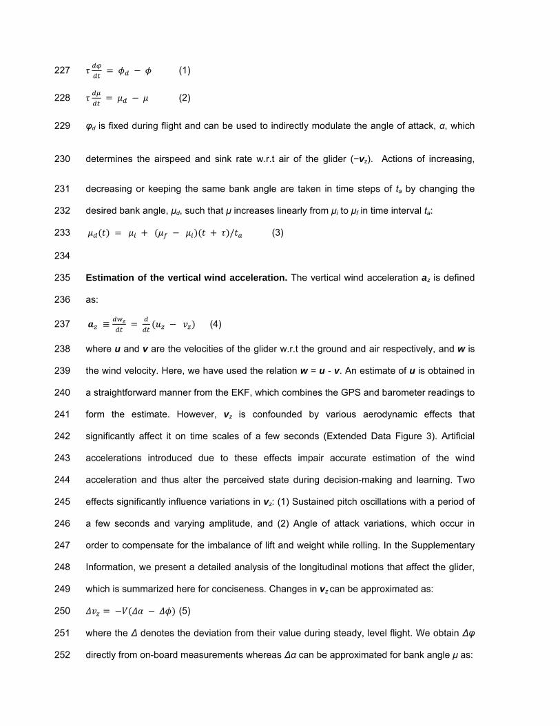
desired bank angle, μd, such that μ increases linearly from μi to μf in time interval ta: 232 ( ) = + ( − )( + )/ (3) 233

234

Estimation of the vertical wind acceleration. The vertical wind acceleration az is defined 235

as: 236 ≡ = ( − ) (4) 237

where u and v are the velocities of the glider w.r.t the ground and air respectively, and w is 238

the wind velocity. Here, we have used the relation w = u - v. An estimate of u is obtained in 239

a straightforward manner from the EKF, which combines the GPS and barometer readings to 240

form the estimate. However, vz is confounded by various aerodynamic effects that 241

significantly affect it on time scales of a few seconds (Extended Data Figure 3). Artificial 242

accelerations introduced due to these effects impair accurate estimation of the wind 243

acceleration and thus alter the perceived state during decision-making and learning. Two 244

effects significantly influence variations in vz: (1) Sustained pitch oscillations with a period of 245

a few seconds and varying amplitude, and (2) Angle of attack variations, which occur in 246

order to compensate for the imbalance of lift and weight while rolling. In the Supplementary 247

Information, we present a detailed analysis of the longitudinal motions that affect the glider, 248

which is summarized here for conciseness. Changes in vz can be approximated as: 249 = − ( − ) (5) 250

where the ∆ denotes the deviation from their value during steady, level flight. We obtain ∆φ 251

directly from on-board measurements whereas ∆α can be approximated for bank angle μ as: 252

≈ ( − )( − 1) (6) 253

where α0 is the angle of attack at steady, level flight and αi is a parameter which depends on 254

the geometry and the angle of incidence of the wing. The constant pre-factor (α0 - αi) is 255

inferred from experiments. Measurements of uz together with the estimate of ∆vz are now 256

used to estimate the vertical wind velocity wz up to a constant term, which can be ignored as 257

it does not affect az. The vertical wind acceleration az is then obtained by taking the 258

derivative of wz and is further smoothed using an exponential smoothing kernel of time scale 259

σa (Extended Data Figure 4). 260

261

Estimation of vertical wind velocity gradients across the wings. Spatial gradients in the 262

vertical wind velocity induce a roll-wise torque on the plane, which we estimate using the 263

deviation of the measured bank angle from the expected bank angle. The total roll-wise 264

torque on the plane has contributions from three sources – (1) the feedback control of the 265

plane, (2) spatial gradients in the wind including turbulent fluctuations, and (3) roll-wise 266

moments created due to various aerodynamic effects. Here, we follow an empirical 267

approach: we note that the latter two contributions perturb the evolution of the bank angle 268

from equation (2). We can then write an effective equation, 269 = + ( ) + ( ) (7) 270

where ω(t) and ωaero(t) are contributions to the roll-wise angular velocity due to the wind and 271

aerodynamic effects respectively. We empirically find four major contributions to ωaero: (1) 272

the dihedral effect, which is a stabilizing moment due to the effects of sideslip on a dihedral 273

wing geometry, (2) the overbanking effect, which is a destabilizing moment that occurs 274

during turns with small radii, (3) trim effects, which create a constant moment due to 275

asymmetric lift on the two wings, and (4) a loss of rolling moment generated by the ailerons 276

when rolling at low airspeeds. We quantify the contributions from the four effects and model 277

their dependence on the bank angle (see Supplementary Information for more details on 278

modeling and calibration). A estimate of ω is then obtained as: 279

= − − (8) 280

Finally, an exponential smoothing kernel is applied to obtain a smoothed ω (Extended Data 281

Figure 5). 282

283

Design of the learning module. The navigational component of the glider is modeled as a 284

Markov Decision Process (MDP), closely following the implementation used in ref. 20. The 285

Markovian transitions are discretized in time into intervals of size ta. The state space consists 286

of the possible values taken by az, ω and μ. To make the learning feasible within 287

experimental constraints and to maintain interpretability, we use a simple tile coding scheme 288

to discretize our state space: continuous values of az and ω are each discretized into three 289

states (+,0,−), partitioned by thresholds ± Ka, ± Kω respectively. The thresholds are set at ± 290

0.8 times the standard deviation of az and ω. Since the width of the distributions of az and ω 291

can vary across days, the data obtained on a particular day is normalized by the standard 292

deviation calculated for that day. In effect, the filtration threshold to detect a signal against 293

turbulent “noise” is higher on days with more turbulence. The consequence is that the 294

behavior of the learned strategy could change across days, adapting to the recent statistics 295

of the environment. The bank angle takes five possible values – 0◦, ± 15◦, ± 30◦, while the 296

three possible actions allow for increasing, decreasing by 15◦ or keeping the same bank 297

angle. In summary, we have a total of 3 × 3 × 5 = 45 states in the state space and 3 actions 298

in the action space. 299

300

We choose the local vertical wind acceleration az obtained in the next time step as the 301

reward function. The choice of az as an appropriate reward signal is motivated by 302

observations made in simulations from ref. 20. In the Supplementary Information, we show 303

that the obtained policy using az as the reward function is equivalent to a policy that also 304

maximizes the expected gain in height. 305

306

Learning the thermalling strategy in the field. Data collected in the field is split into 307

(s,a,s',r) quadruplets containing the current state s, the current action a, the next state s' and 308

the obtained reward r, which are pooled together to obtain the transition matrix T(s'|s,a) and 309

reward function R(s,a). Value iteration methods are used to estimate the Q values from T 310

and R. The learning process is offline and off-policy; specifically, we begin training with a 311

‘random’ policy that takes the three possible actions with equal probability irrespective of the 312

current state as our behavioral policy, which was used for 12 out of the 15 days of training. 313

For the other days, a softmax policy7 with temperature set to 0.3 was used. For softmax 314

training, the Q values were first estimated from the data obtained in the previous days and 315

then normalized by the difference between the maximum and minimum Q values over the 316

three possible actions at a particular state, as described in ref. 20. 317

318

Using a fixed, random policy as our behavioral policy slows learning as state-action pairs 319

that rarely appear in the final policy are still sampled. On the other hand, calibrating the 320

parameters necessary for the unbiased measurement of az and ω (see Supplementary 321

Information) is performed simultaneously with learning, which considerably reduces the 322

number of days required in the field. Importantly, offline learning permits us to continuously 323

monitor the variance of the estimated Q values by bootstrapping from the set E of 324

accumulated (s,a,s′,r) quadruplets up to a particular point. Specifically, |E| samples are 325

drawn with replacement from E and Q values are obtained for each state-action pair via 326

value iteration. The steps are repeated and the average of the bootstrapped standard 327

deviations in Q over all the state-action pairs is used as a measure of learning progress, as 328

shown in Figure 2A. 329

330

We expect certain symmetries in the transition matrix and the reward function, which we 331

exploit in order to expedite our learning process. Particularly, we note that the MDP is 332

invariant to an inversion of sign in the bank angle μ → −μ. This transforms a state as (az,ω,μ) 333

→ (az,-ω,-μ) and inverts the action from that of increasing the bank angle to decreasing the 334

bank angle and vice-versa. We symmetrize T and R as 335

= (9) 336

= (10) 337

where + and − denote the obtained values and those computed by applying the inverting 338

transformation respectively. Finally, Tsym and Rsym are used to obtain a symmetrized Q 339

function, which results in a symmetric policy as shown in Figure 2b. To conveniently obtain 340

the policy that uses only az (Figure 3d), the above procedure is repeated with the threshold 341

for ω (Kω) set to infinity. 342

343

Testing the performance of the learned policy in the field. To obtain the data shown in 344

Figure 3b, the glider is first sent autonomously to an arbitrary but fixed location 250 m above 345

ground level. The learned thermalling policy is then turned on and the mean climb rate i.e., 346

the total height gained divided by the total time, is measured over a 3-minute interval. To 347

obtain the control data, the glider instead follows a random policy, which takes the three 348

possible actions with equal probability. The trials where we observe little to no atmospheric 349

convection were filtered out by imposing a threshold on the standard deviation of the vertical 350

wind velocity over the 3-minute trial. In Extended Data Figure 6, we show the distribution of 351

the standard deviation in wz collected from ~240 3-minute trials over 9 days. Trials below the 352

threshold chosen as the 25th percentile mark (red, dashed line) are not used for our 353

analysis. 354

355

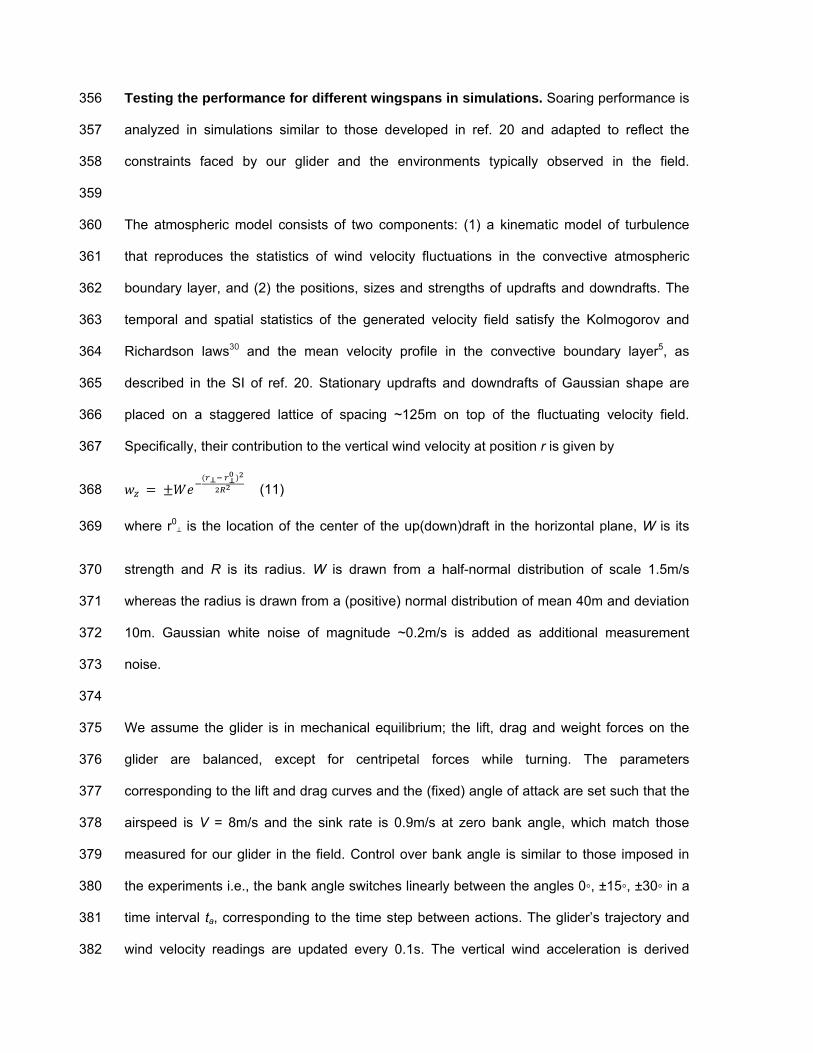
Testing the performance for different wingspans in simulations. Soaring performance is 356

analyzed in simulations similar to those developed in ref. 20 and adapted to reflect the 357

constraints faced by our glider and the environments typically observed in the field. 358

359

The atmospheric model consists of two components: (1) a kinematic model of turbulence 360

that reproduces the statistics of wind velocity fluctuations in the convective atmospheric 361

boundary layer, and (2) the positions, sizes and strengths of updrafts and downdrafts. The 362

temporal and spatial statistics of the generated velocity field satisfy the Kolmogorov and 363

Richardson laws30 and the mean velocity profile in the convective boundary layer5, as 364

described in the SI of ref. 20. Stationary updrafts and downdrafts of Gaussian shape are 365

placed on a staggered lattice of spacing ~125m on top of the fluctuating velocity field. 366

Specifically, their contribution to the vertical wind velocity at position r is given by 367

= ± ( ) (11) 368

where r0⊥ is the location of the center of the up(down)draft in the horizontal plane, W is its 369

strength and R is its radius. W is drawn from a half-normal distribution of scale 1.5m/s 370

whereas the radius is drawn from a (positive) normal distribution of mean 40m and deviation 371

10m. Gaussian white noise of magnitude ~0.2m/s is added as additional measurement 372

noise. 373

374

We assume the glider is in mechanical equilibrium; the lift, drag and weight forces on the 375

glider are balanced, except for centripetal forces while turning. The parameters 376

corresponding to the lift and drag curves and the (fixed) angle of attack are set such that the 377

airspeed is V = 8m/s and the sink rate is 0.9m/s at zero bank angle, which match those 378

measured for our glider in the field. Control over bank angle is similar to those imposed in 379

the experiments i.e., the bank angle switches linearly between the angles 0◦, ±15◦, ±30◦ in a 380

time interval ta, corresponding to the time step between actions. The glider’s trajectory and 381

wind velocity readings are updated every 0.1s. The vertical wind acceleration is derived 382

assuming that the glider directly reads the local vertical wind velocity. The vertical wind 383

velocity gradients across the wings are estimated as the difference between the vertical wind 384

velocities at the two ends of the wings. The readings are smoothed using exponential 385

smoothing kernels; the smoothing parameters in experiments are chosen to coincide with 386

those that yield the most gain in height in simulations. 387

388

Estimation of the noise in gradient sensing due to atmospheric turbulence. The cues 389

az and ω measure the gradients in the vertical wind velocity along and perpendicular to the 390

heading of the glider. Updrafts and downdrafts are relatively stable structures in a varying 391

turbulent environment. Thermal detection through gradient sensing constitutes a 392

discrimination problem of deciding whether a thermal is present or absent given the current 393

az and ω. We estimate the magnitude of turbulent ‘noise’ that unavoidably accompanies 394

gradient sensing. Intuitively, turbulent fluctuations in the atmospheric boundary layer (ABL) 395

are made up of eddies of different length scales, with the largest being the size of the height 396

of the ABL. Energy is transferred from larger, stronger eddies to smaller, weaker eddies, and 397

eventually dissipates at the centimeter scale due to viscosity in the bulk and the boundaries. 398

In the Supplementary Information, we present an explicit calculation of the signal to noise 399

ratio for ω estimation taking into account the effect of turbulent eddies on the statistics of 400

noise. Below, we give simple scaling arguments and refer to the Supplementary Information 401

for further details. 402

403

A glider moving at an airspeed V and integrating over a time scale T averages az over a 404

length VT. For V much larger than the velocity scale of the eddies, which is typically the 405

case, the decorrelation of wind velocities is due to the glider’s motion; the eddies themselves 406

can be considered to be frozen in time. The magnitude of the spatial fluctuations across the 407

eddy of this size scales according to the Richardson-Kolmogorov law30 as ~ (VT)1/3. The 408

mean gradient signal when going up the gradient is ~ (VT); the resultant signal to noise ratio 409

in az scales as (VT)2/3. 410

411

Similar arguments are applicable for ω measurements. In this case, the signal to noise ratio 412

has an additional dependence on the wingspan l. The dominant contribution to the noise 413

comes from eddies of size l, whose strength scales as l1/3. As the glider moves a distance 414

VT, for l ≪ VT, it traverses VT/l distinct eddies of size l. Consequently, the noise is averaged 415

out by a factor (VT/l)−1/2, corresponding to the VT/l independent measurements. Multiplying 416

these two factors, the averaged noise is ~ l5/6(VT)-1/2. Since the mean gradient (i.e., the 417

signal) is ~ l, the signal to noise ratio is then ~ l1/6(VT)1/2. 418

419

From the above arguments and dimensional considerations, we get order-of-magnitude 420

estimates of the SNR for az and ω estimation: 421 ( ) ∼ / / / (12) 422

( ) ∼ / / / / (13) 423

where W is the strength of the thermal, R is its radius, w is the magnitude of turbulent 424

vertical wind velocity fluctuations and L is the length scale of the ABL. For the SNR 425

estimates presented in the text, we use W = 2m/s, R = 50m, l = 2m, V = 8m/s, T = 3 s, L = 1 426

km. The values of V and T correspond to the airspeed of the glider in experiments and the 427

time scale between actions during learning respectively. 428

429

Data availability. The data that support the findings of this study are available from the 430

corresponding author upon reasonable request. 431

References

1. Newton I., Migration Ecology of Soaring Birds, Elsevier, 1st edition, 2008.

2. Shamoun-Baranes, J., Leshem, Y., Yom-tov, Y. and Liechti, O., Differential Use of

Thermal Convection by Soaring Birds Over Central Israel, The Condor, 105(2): 208-

218, 2003.

3. Weimerskirsch, H., Bishop, C., Jeanniard-du-Dot, T., Prudor, A. and Sachs, G.,

Frigate birds track atmospheric conditions over months-long transoceanic flights,

Science, 353(6294): 74-78, 2016.

4. Pennycuick, C. J., Thermal Soaring Compared in Three Dissimilar Tropical Bird

Species, Fregata Magnificens, Pelecanus Occidentals and Coragyps Atratus, J. Exp.

Biol., 102:307-325, 1983.

5. Garrat, J. R., The Atmospheric Boundary Layer, Cambridge Atmospheric and Space

Science Series, Cambridge University Press, 1994.

6. Lenschow, D. H., & Stephens, P. L., The role of thermals in the atmospheric

boundary layer, Boundary-Layer Meteorology, 19:509-532, 1980.

7. Sutton, R. S., & Barto, A. G., Reinforcement Learning: An Introduction, MIT Press,

1st edition, 1998.

8. Tesauro, G., Temporal difference learning and TD-Gammon, Commun ACM, 38: 58–

68, 1995.

9. Silver, D. et al, Mastering the game of Go without human knowledge, Nature,

550:354-359, 2017.

10. Mnih, V. et al, Human-level control through deep reinforcement learning, Nature,

518:529–533, 2014.

11. Kim, H. J., Jordan, M. I., Sastry, S., and Ng, A., Autonomous Helicopter Flight via

Reinforcement Learning, Advances in Neural Information Processing Systems, 16,

2003.

12. Levine, S., Finn, C., Darrell, T. and Abbeel, P., End-to-End Training of Deep

Visuomotor Policies, Journal of Machine Learning Research, 17:1-40, 2016.

13. Allen, M. J. & Lin, V., Guidance and Control of an Autonomous Soaring UAV,

Proceedings of the AIAA Aerospace Sciences Meeting, (American Institute of

Aeronautics and Astronautics, Reston, VA), AIAA Paper 2007-867.

14. Edwards, D. J., Implementation Details and Flight Test Results of an Autonomous

Soaring Controller, AIAA Guidance, Navigation and Control Conference and Exhibit,

2008.

15. Edwards, D. J., Autonomous Soaring: The Montague Cross Country Challenge

Doctorate theses, North Carolina State University, Aerospace Engineering, Raleigh,

North Carolina, 2010.

16. Ákos, Z., Nagy, M., Leven, S., and Vicsek, T., Thermal soaring flight of birds and

unmanned aerial vehicles. Bioinspiration & Biomimetics, 5(4), 045003, 2010.

17. Doncieux, S., Mouret, J. B. and Meyer J-A., Soaring behaviors in UAVs : 'animat'

design methodology and current results. In 7th European Micro Air Vehicle

Conference (MAV07), Toulouse, 2007. �

18. Wharington, J. and Herszberg, I., Control of a high endurance unmanned aerial ve-

�hicle, Proceedings of the 21st Congress of International Council of the Aeronautical

Sciences (International Council of the Aeronautical Sciences, Bonn, Germany),

Paper 98-3.7.1, 1998.

19. Chung J. J., Lawrance, N. R. J. and Sukkarieh, S, Learning to soar: Resource-

constrained exploration in reinforcement learning, The International Journal of

Robotics Research, 34(2):158-172, 2014.

20. Reddy, G., Celani, A., Sejnowski, T. and Vergassola, M., Learning to soar in

turbulent environments, Proc. Natl. Acad. Sci., 113(33): E4877-E4884, 2016.

21. Yeung, P. K. and Pope, S. B., Lagrangian statistics from direct numerical simulations

of isotropic turbulence, J. Fluid. Mech., 207:531-586, 1989.

22. Voth, G. A., La Porta, A., Crawford, A. M., Alexander, J., and Bodenschatz, E.,

Measurement of particle accelerations in fully developed turbulence, J. Fluid. Mech.,

469:121-160, 2002.

23. Tennekes, H. and Lumley, J. L., A first course in turbulence, MIT Press, 1972.

24. Reichmann, H., Cross-Country Soaring, Thomson Publications, Santa Monica, CA,

1988.

25. Ng, A. Y., Harada, D., and Russell, S. J., Policy Invariance Under Reward

Transformations: Theory and Application to Reward Shaping, Proc. of the 16th

International Conference on Machine Learning, P278-287, 1999.

26. MacCready, P. B. J., Optimum airspeed selector, Soaring, 1958(1): 10–11, 1958.

27. Horvitz, N. et al., The gliding speed of migrating birds: Slow and safe or fast and

risky? Ecology Letters, 17(6):670–679, 2014.

28. Cochrane, J. H., MacCready theory with uncertain lift and limited altitude, Technical

Soaring, 23:88–96, 1999.

29. ArduPilot, www.ardupilot.org, (2018).

30. Frisch, U., Turbulence: The Legacy of A. N. Kolmogorov, Cambridge University

Press, 1995.

Supplementary Information

Supplementary Information is linked to the online version of the paper at

www.nature.com/nature.

Acknowledgements

This work was supported by Simons Foundation Grant 340106 (to M.V.).

Author Contributions

All authors were involved in designing the study and drafting the final manuscript. G.R. and

J.W.N. performed the experiments and analyzed the data. G.R., A.C. and M.V. contributed

to the theoretical results.

Author Information

Reprints and permissions information is available at www.nature.com/reprints.

The authors declare no competing financial interests.

Correspondence and requests for materials should be addressed to M.V

(massimo@physics.ucsd.edu).

Extended Data Legends

Extended Data Table 1: Parameter values.

Extended Data Figure 1: Sample trajectories obtained in the field. The three-

dimensional view and top view of the glider’s trajectory as it executes the learned thermalling

strategy (labeled ‘s’) or a random policy that takes actions with equal probability (labeled ‘r’).

The trajectories are colored with the instantaneous vertical ground velocity (uz). The green

(red) dot shows the start (end) point of the trajectory. Trajectories s1, s2 and r1 last for 3

minutes each, whereas s3 lasts for ~8 minutes.

Extended Data Figure 2: Force-body diagram of a glider. The forces on a glider and the

definitions of the various angles that determine the glider's motion.

Extended Data Figure 3: Modeling the longitudinal motion of the glider. (a) A sample

trajectory of a glider's pitch and its vertical velocity w.r.t ground uz in a case where the

feedback control over the pitch is reduced in order to exaggerate the pitch oscillations. The

blue line shows the measured uz and the orange line is uz obtained after subtracting the

contributions from longitudinal motions of the glider (see Supplementary Information). (b)

The blue line shows the average change in uz when a particular action is taken (labeled

above each panel), averaged over n three-second intervals. The 13 panels correspond to

the 13 possible bank angle changes from the angles 0o, ±15o, and ±30o by increasing,

decreasing the bank angle by 15o or keeping the same angle. The green, dashed line shows

the prediction from the model whereas the orange line is the estimated wz. The axis on the

right shows the averaged pitch as a red, dashed line.

Extended Data Figure 4: The estimated vertical wind acceleration is unbiased after

accounting for the glider’s longitudinal motion. (a) The averaged vertical wind

acceleration, az in units of its standard deviation az, plotted as in Extended Data Figure 3b, is

shown in orange with (blue line) and without (orange line) accounting for the glider's

longitudinal motions. The axis on the right shows the airspeed as a green, dashed line. (b)

The PDFs (probability density functions) of az for the different bank angle changes. The

black, dashed line shows the median.

Extended Data Figure 5: The estimated roll-wise torque is unbiased after accounting

for the effects of feedback control and glider aerodynamics. (a) The averaged evolution

of the bank angle shown as in Extended Data Figure 3b. The blue line shows the measured

bank angle and the dashed, orange line shows the best-fit line obtained from simultaneously

fitting the 13 blue curves to the prediction (see Supplementary Information). (b) The PDFs

(probability density functions) of the roll-wise torque ω (in units of its standard deviation) for

the different bank angle changes. The black, dashed line shows the median value.

Extended Data Figure 6: The distribution of the strength of vertical currents observed

in the field. The root-mean-square vertical wind velocity measured in the field is pooled from

~240 3-minute trials collected over 9 days. The dashed, red line shows the threshold

criterion imposed when measuring the performance of the strategy in the field (see

Methods).

a

0 50 100Time(s)

-2

2

0 (o /s)

Time(s)0 50 100

-30

-15

0

15

30

(o )

1.5

0

-1.5

wz (

m/s

)

a z (m

/s2 )

0

-0.2

0.2

c

d

b

2 m

30o15o0o-15o-30o

+

0

-

az

+0-

+0-

+0-

-15o

0o

15o

101 102 103

Training time (minutes)

0

0.5

1

Std

. dev

.(Q)

aa b

-1

0.5

2

u z (m

/s)

200

300

400

500

600

700

200

400

X (m)

200

400

Y (m)

Z (m)

start

end

Random az az +

0

-0.4

-0.8Mea

n cl

imb

rate

(m/s

)

Wingspan l (m)2 6 10

a c

d

0 5 10 15Wingspan l (m)

0

4

8

1

2

4

10-3 10-1 101Sig

nal-t

o-no

ise

ratio

az

~ l1/6

Clim

b ra

te (m

/s)

-1

1

0

-2

Random Strategy

b