Introduction to a few basic concepts in thermoelectricity

Giuliano Benenti

Center for Nonlinear and Complex SystemsUniv. Insubria, Como, Italy

1

Irreversible thermodynamic

Irreversible thermodynamics based on the postulates of equilibrium electrostatics plus the postulate of time-reversal symmetry of physical laws (if time t is replaced by -t and simultaneously applied magnetic field B by -B)

The thermodynamic theory of irreversible processes is based on the Onsager Reciprocity Theorem

2

Thermodynamic forces and fluxesIrreversible processes are driven by thermodynamic forces (or generalized forces or affinities) Xi

Fluxes Ji characterize the response of the system to the applied forces

Entropy production rate given by the sum of the products of each f lux with i ts associated thermodynamic force

S = S(U, V,N1, N2, ...) = S(E0, E1, E2, ...)

dS

dt=

�

k

∂S

∂Ek

dEk

dt=

�

k

XkJk

3

Linear responsePurely resistive systems: fluxes at a given instant depend only on the thermodynamic forces at that instant (memory effects not considered)

Fluxes vanish as thermodynamic forces vanish

Ji =�

j

LijXj

Linear (and purely resistive) processes:

Lij Onsager coefficients (first-order kinetic coefficients) depend on intensive quantities (T,P,µ,...)

Ji =�

j

LijXj +12

�

jk

LijkXjXk + ...

Phenomenological linear Ohm’s, Fourier’s, Fick’s laws4

Onsager-Casimir reciprocal relations

Relationship of Onsager theorem to time-reversal symmetry of physical laws

Lij(B) = Lji(−B)

Consider delayed correlation moments of fluctuations (for simplicity without applied magnetic fields)

δEj(t) ≡ Ej(t)− Ej , �δEj� = 0,

�δEj(t)δEk(t + τ)� = �δEj(t)δEk(t − τ)� = �δEj(t + τ)δEk(t)�

limτ→0

�δEj(t)

δEk(t + τ)− δEk(t)τ

�= lim

τ→0

�δEj(t + τ)− δEj(t)

τδEk(t)

�

�δEjδEk� = �δEjδEk�

5

Assume that fluctuations decay is governed by the same linear dynamical laws as are macroscopic processes

δEk =�

l

LklδXl

�

l

Lkl�δEjδXl� =�

l

Ljl�δXlδEk�

Assume that the fluctuation of each thermodynamic force is associated only with the fluctuation of the corresponding extensive variable

�δEjδXl� = 0 if l �= j

6

Steady state heat to work conversion

Stochastic baths: ideal gases at fixed temperature

and chemical potential

X2 = ∆β ≈ −∆T/T 2

7

Restrictions from thermodynamics

Onsager relation:

Positivity of entropy production:

Let us consider the time-symmetric case

dρ

dt= JρX1 + JqX2 ≥ 0

8

Onsager and transport coefficients

G =�

Jρ

∆µ/e

�

∆T=0

⇒ G =e2

TLρρ

Ξ =�

Jq

∆T

�

Jρ=0

⇒ Ξ =1

T 2

detLLρρ

Note that the positivity of entropy production implies that the (isothermal) electric conductance G>0 and the thermal conductance Ξ>0

S =�

∆µ/e

∆T

�

Jρ=0

⇒ S = − 1eT

Lρq

Lρρ

9

Seebeck and Peltier coefficients

Seebeck and Peltier coefficients are trivially related by Onsager reciprocal relations (when time symmetry is not broken)

S =�

∆µ/e

∆T

�

Jρ=0

⇒ S = − 1eT

Lρq

Lρρ

Π =�

Jq

eJρ

�

∆T=0

=Lqρ

eLρρ=

Lρq

eLρρ= TS

10

Local equilibrium

Under the assumption of local equilibrium we can write phenomenological equations with ∇T and ∇µ rather than ΔT and Δµ

In this case we connect Onsager coefficients to electric and thermal conductivity rather than to conductances

σ =�

Jρ

∇µ/e

�

∇T=0

, κ =�

Jq

∇T

�

Jρ=0

11

Kinetic equations in terms of transport coefficients

By eliminating ∇µ we obtain

The Seebeck coefficient can be understood as the entropy transported (per unit charge) by the electron flow. The last term is independent of the particle flow

12

Energy and heat representations

X2 = ∆β ≈ −∆T/T 2

Jρ = LρρX1 + LρuX2

Ju = LuρX1 + LuuX2

X1 = −∆(βµ)X2 = X2

Jq = TJs = Ju − µJρ

13

Steady state power generation efficiency

14

Maximum efficiency

Find the maximum of η over X1, for fixed X2 (i.e., over the applied voltage ΔV for fixed temperature difference ΔT)

15

Thermoelectric figure of merit

16

ZT diverges iff the Onsager matrix is ill-conditioned, that is, the condition number:

diverges

In such case the system is singular (strong-coupling limit):

(the ratio Jq/Jρ is independent of the applied voltage and temperature gradients)

17

Maximum refrigeration efficiency

ZT is the figure of merit also for refrigeration

18

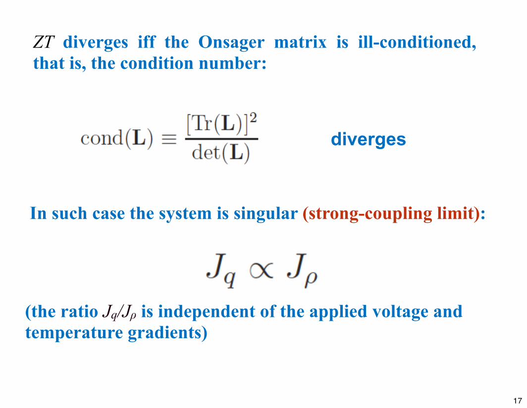
Finite time thermodynamics

Carnot efficiency obtained in the limit of quasi-static (reversible) processes, so that the extracted power reduces to zero.

Finite time thermodynamics (endoreversible thermodynamics) considers finite time (Carnot) cycles; the efficiency at the maximum output power is an important concept

19

Efficiency at maximum powerFor finite time Carnot cycles the efficiency at the maximum output power is given (under some conditions) by the so-called Curzon-Ahlborn efficiency (Chambadal-Novikov efficiency)

20

Curzon-Ahlborn efficiency

Optimum power delivered by the engine:

The CA efficiency is not a generic bound for the efficiency at maximum power; yet it describes the efficiency of actual thermal plants quite well

Efficiency at the maximum output power is given by the Curzon-Ahlborn efficiency

21

Linear response Curzon-Ahlborn upper bound

The CA efficiency is a universal upper bound within linear response

Within linear response, the output power

is maximum when

22

Maximum output power

Efficiency at maximum power

Both maximum efficiency and efficiency at maximum power are monotonous growing functions of the thermoelectric figure of merit ZT

23

Charge current

Non-interacting systems, Landauer-Büttiker formalism

Heat current from reservoir α

Jq.α =1h

� ∞

−∞dE(E − µα)τ(E)[fL(E)− fR(E)]

24

Onsager coefficients

The Onsager coefficients are obtained from the linear expansion of the charge and thermal currents

25

Wiedemann-Franz law

Phenomenological law: the ratio of the thermal to the electrical conductivity of a great number of metals is directly proportional to the temperature, with a proportionality factor which is to a good accuracy the same for all metals.

Lorenz number

26

Sommerfeld expansionThe Wiedemann-Franz law can be derived for low-temperature non-interacting systems both within kinetic theory or Landauer-Büttiker approaches

In both cases it is substantiated by Sommerfeld expansion

We assume smooth transmission functions τ(E) in the neighborhood of E=µ

Jq.α =1h

� ∞

−∞dE(E − µα)τ(E)[fL(E)− fR(E)]

27

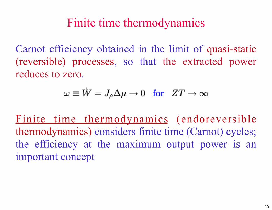
To lowest order in kBT/EF

Assuming LρρLqq>>(Lρq)2

To the leading order (second order) in kBT/EF

Wiedemann-Franz law:

28

Wiedemann-Franz law and thermoelectric efficiency

Wiedemann-Franz law derived under the condition LρρLqq>>(Lρq)2 and therefore

Wiedemann-Franz law violated in - low-dimensional interacting systems that exhibit non-Fermi liquid behavior- small systems where transmission can show significant energy dependence

29

(Violation of) Wiedemann-Franz law in small systems

30

Cutler-Mott formula

For non-interacting electrons

Electron and holes contribute with opposite signs: we want sharp, asymmetric transmission functions to have large thermopowers (ex: resonances, Anderson QPT, see Imry and Amir, 2010), violation of WF, large ZT.

Consider smooth transmissions

31

If transmission is possible only inside a tiny energy window around E=E✶ then

Thermoelectric efficiency

32

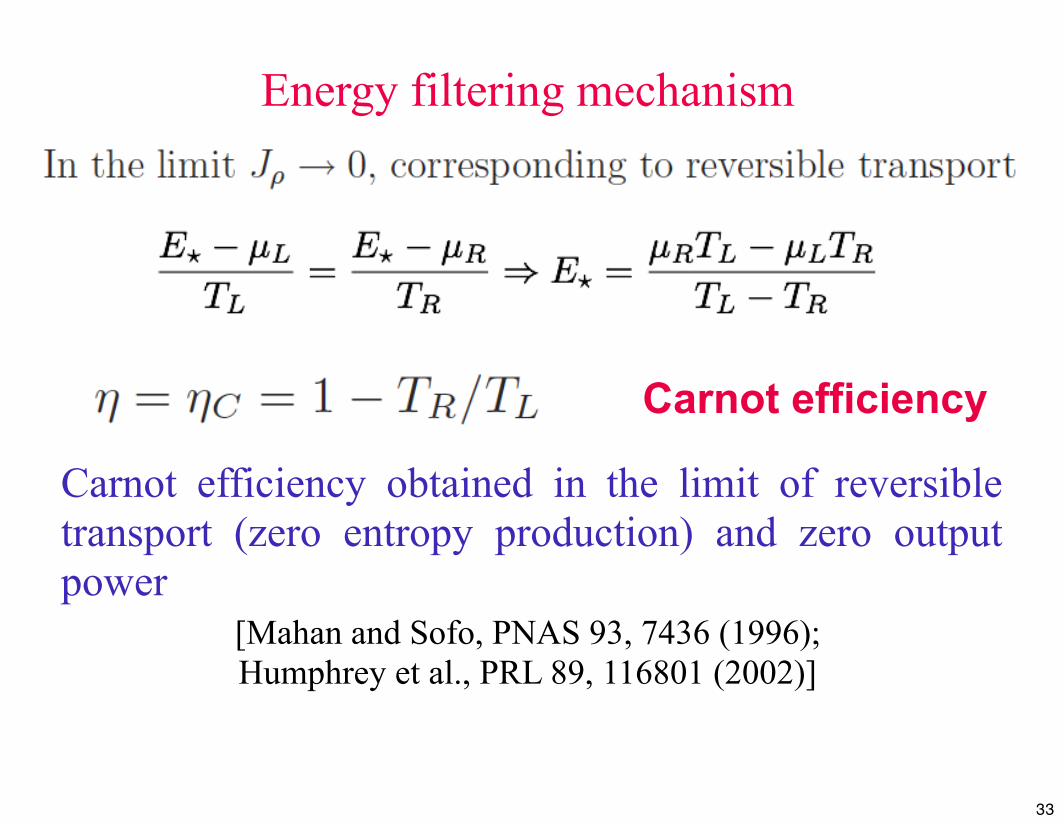
Carnot efficiency

[Mahan and Sofo, PNAS 93, 7436 (1996); Humphrey et al., PRL 89, 116801 (2002)]

Energy filtering mechanism

Carnot efficiency obtained in the limit of reversible transport (zero entropy production) and zero output power

33

Interacting systems, Green-Kubo formulaThe Green-Kubo formula expresses linear response transport coefficients in terms of dynamic correlation functions of the corresponding current operators, cal- culated at thermodynamic equilibrium

Non-zero generalized Drude weights signature of ballistic transport

34

Conservation laws and thermoelectric efficiencySuzuki’s formula for finite-size Drude weights

Qn relevant (i.e., non-orthogonal to charge and thermal currents), mutually orthogonal conserved quantities

35

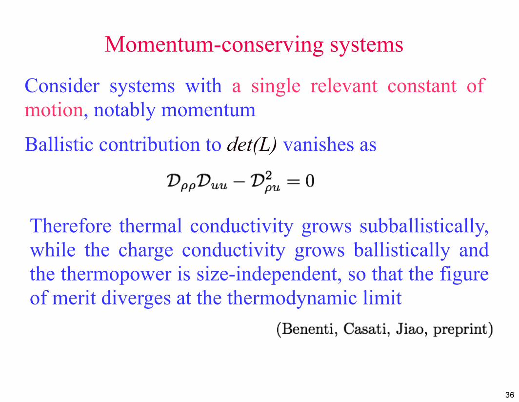
Momentum-conserving systems

Consider systems with a single relevant constant of motion, notably momentum

Ballistic contribution to det(L) vanishes as

Therefore thermal conductivity grows subballistically, while the charge conductivity grows ballistically and the thermopower is size-independent, so that the figure of merit diverges at the thermodynamic limit

36

Example: 1D interacting classical gas

Consider a one dimensional gas of elastically colliding particles with unequal masses: m, M

ZT =1

injection rates

ZT depends on the system size

37

Anomalous thermal transport

ZT =σS2

kT

(Saito, G.B., Casati, Chem. Phys. 375, 508 (2010))

38