University of Colorado, BoulderCU Scholar

Science Boot Camp for Librarians – West University Libraries

Summer 6-20-2013

GIS Modeling of the Natural and HumanEnvironmentBarbara ButtenfieldUniversity of Colorado Boulder

Follow this and additional works at: http://scholar.colorado.edu/sciboot

This Article is brought to you for free and open access by University Libraries at CU Scholar. It has been accepted for inclusion in Science Boot Campfor Librarians – West by an authorized administrator of CU Scholar. For more information, please contact cuscholaradmin@colorado.edu.

Recommended CitationButtenfield, Barbara, "GIS Modeling of the Natural and Human Environment" (2013). Science Boot Camp for Librarians – West. 3.http://scholar.colorado.edu/sciboot/3

GIS Modeling of the Natural and Human Environment

Barbara P. Buttenfield

Director, Meridian Research Lab

Department of Geography

University of Colorado – Boulder

babs@colorado.edu

Science Literacy Boot Camp, CU-Boulder, 20 June 2013

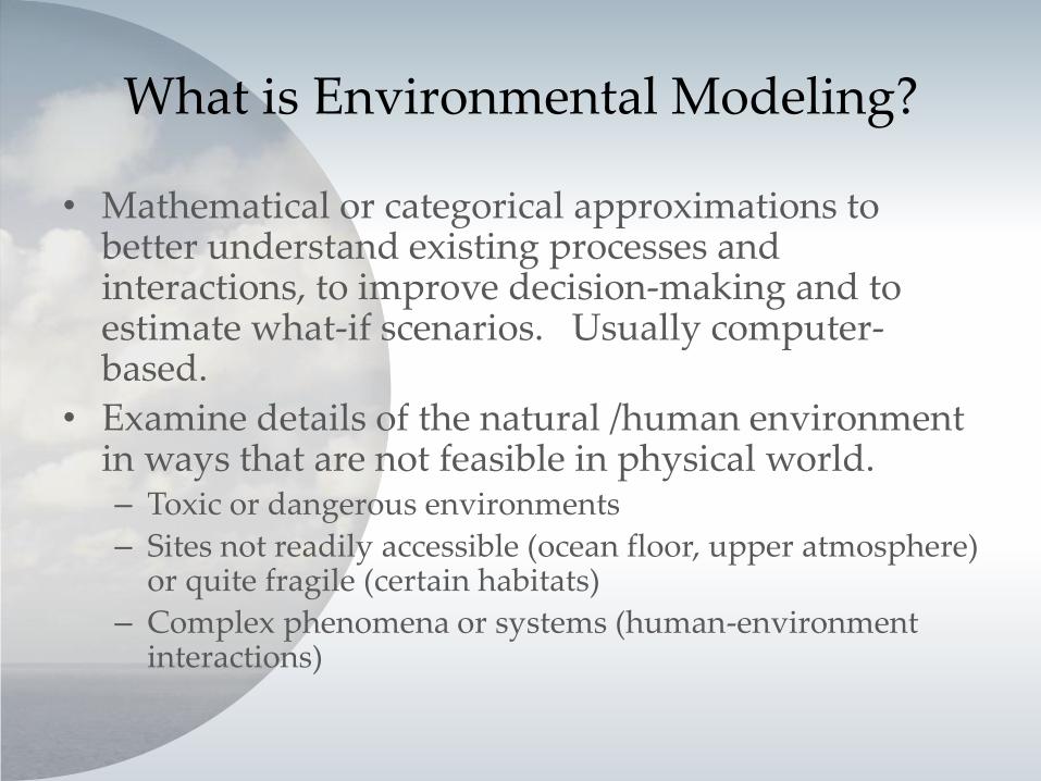
What is Environmental Modeling?

• Mathematical or categorical approximations to better understand existing processes and interactions, to improve decision-making and to estimate what-if scenarios. Usually computer-based.

• Examine details of the natural /human environment in ways that are not feasible in physical world. – Toxic or dangerous environments

– Sites not readily accessible (ocean floor, upper atmosphere) or quite fragile (certain habitats)

– Complex phenomena or systems (human-environment interactions)

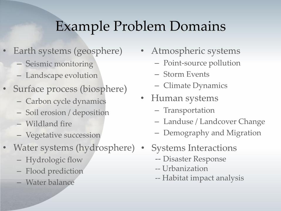
Example Problem Domains

• Earth systems (geosphere)

– Seismic monitoring

– Landscape evolution

• Surface process (biosphere) – Carbon cycle dynamics

– Soil erosion / deposition

– Wildland fire

– Vegetative succession

• Water systems (hydrosphere) – Hydrologic flow

– Flood prediction

– Water balance

• Atmospheric systems – Point-source pollution

– Storm Events

– Climate Dynamics

• Human systems – Transportation

– Landuse / Landcover Change

– Demography and Migration

• Systems Interactions -- Disaster Response -- Urbanization -- Habitat impact analysis

Geospatial Tools for Environmental Modeling

– Ground Instruments: GPS

– Remote Sensing (MODIS, LiDAR, Quickbird, TM)

– GIS (ArcGIS, QGIS, IDRISI, GRASS)

– Statistics (R, Stata, GeoDa)

– Numerical Analysis (Matlab)

– Spatial Analysis (GeoVista Studio)

– Programming Languages (C++, Java, Python)

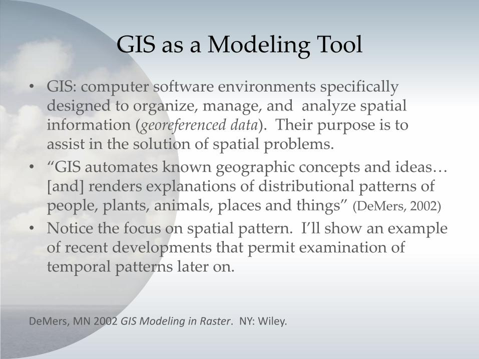
GIS as a Modeling Tool

• GIS: computer software environments specifically designed to organize, manage, and analyze spatial information (georeferenced data). Their purpose is to assist in the solution of spatial problems.

• “GIS automates known geographic concepts and ideas… [and] renders explanations of distributional patterns of people, plants, animals, places and things” (DeMers, 2002)

• Notice the focus on spatial pattern. I’ll show an example of recent developments that permit examination of temporal patterns later on.

DeMers, MN 2002 GIS Modeling in Raster. NY: Wiley.

(psst… What is georeferenced data?)

• GIS data is layered; layers are linked

• Indirect georeferencing

– Layers register to each other (coincident coordinates)

• Direct georeferencing

– At least one layer registers to the planet (map projection)

– Latitude-Longitude

– Geodetic Control

– Terrain data

– Remote sensing

GIS as a Modeling Tool

• GIS modeling makes it possible to explore our world: – To examine, explore, and tinker with landscape

components

– To isolate and or integrate them at selected levels of detail (i.e., resolution or precision)

– To identify what is relevant or superfluous to the question.

All of these activities become possible without requiring physical presence in, and possible consequences to, the places and processes under scrutiny.

The GIS Modeling Process

1. Start with the science What is the question, why is it important to ask, what data is relevant

2. Numeric representation Model Components Equations Algorithm Implementation and Integration of the Components 3. Evaluation / Validation / Sensitivity Analysis

Internal and external assessment, “what-if?” tests

4. Communication of results and reliability Tabular, Discursive, Visualized

+ =? Can surface parameters including landcover and slope be used to establish

a relationship between precipitation and river discharge?

WorldClim gauge stations

Examples of GIS Environmental Models

• Landscape Impacts on Wolf Predation – Student project from my GIS Modeling class

– Environmental biologist, geologist, and cartgrapher

• Refining Census Demography – Master’s Thesis funded by my ongoing NSF grant

– Foreign student exchange program

I’ll walk you through two applications in two different problem domains, highlighting different aspects of GIS modeling of the environment.

Wolf Predation in Yellowstone National Park

• Aidan Beers, Environmental Biology grad student

• Clara Chew, Geology grad student

• Paul Smith, Geography undergrad major

GIS Modeling final project, Fall 2012

(Start with the Science) Research Question

• Since their reintroduction in 1995, gray wolves (Canis lupus) have had an effect on elk populations the Yellowstone National Park ecosystem.

• In their absence, the elk population on the northern range of Yellowstone exceeded 20,000 by some estimates; today that figure is closer to 5,000.

• Wolves are effective pack hunters that usually rely on a chase to secure their prey. But what terrain and landscape factors affect their success rate?

• Evidence from predation suggests that landscape factors are a more important determinant of kills than prey density.

Wo

lf P

red

atio

n

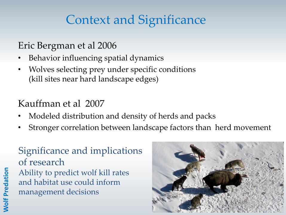
Context and Significance

Eric Bergman et al 2006 • Behavior influencing spatial dynamics

• Wolves selecting prey under specific conditions (kill sites near hard landscape edges)

Kauffman et al 2007 • Modeled distribution and density of herds and packs

• Stronger correlation between landscape factors than herd movement

Wo

lf P

red

atio

n

Significance and implications of research Ability to predict wolf kill rates and habitat use could inform management decisions

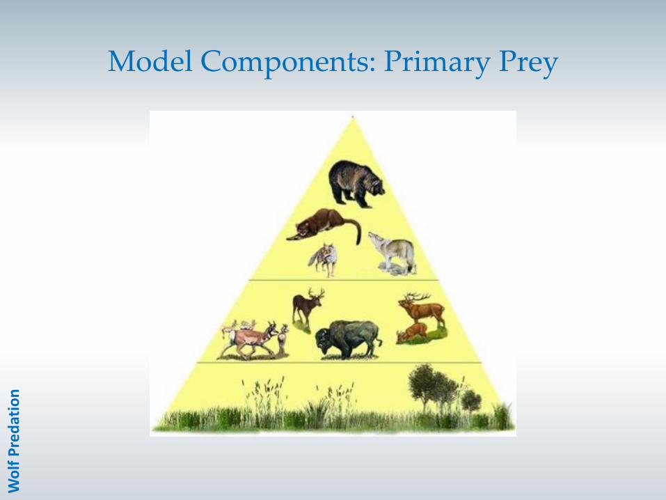
Model Components: Primary Prey

Wo

lf P

red

atio

n

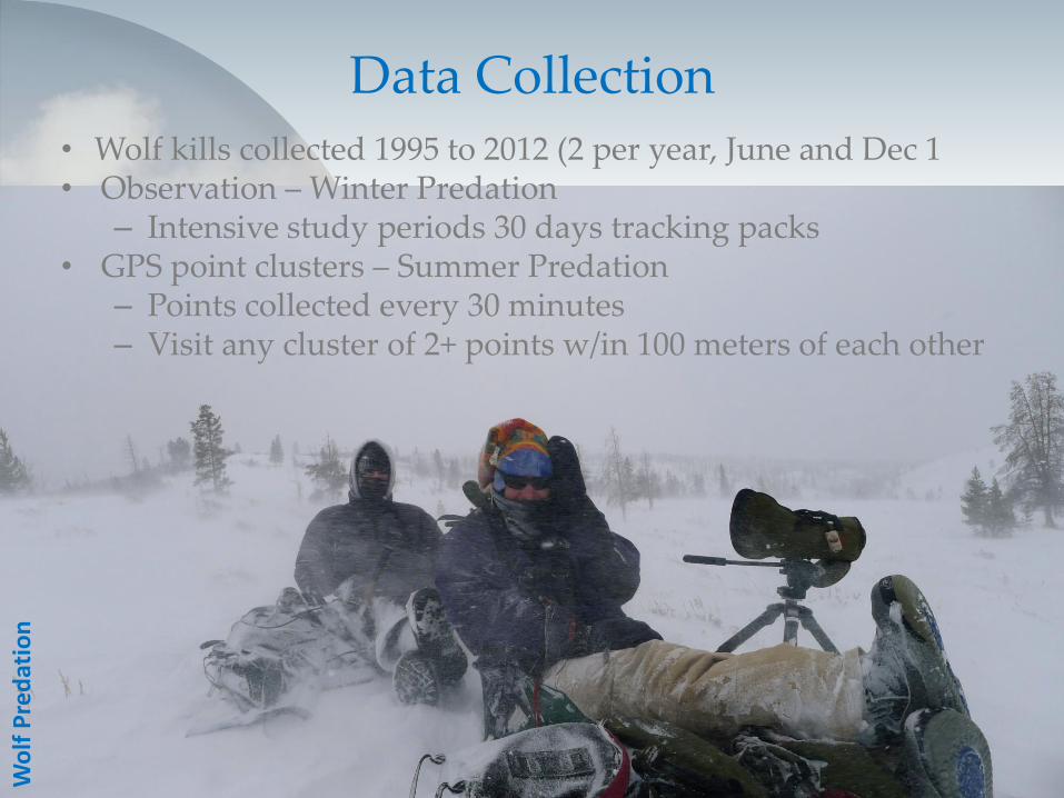
Data Collection • Wolf kills collected 1995 to 2012 (2 per year, June and Dec 1 • Observation – Winter Predation

– Intensive study periods 30 days tracking packs • GPS point clusters – Summer Predation

– Points collected every 30 minutes – Visit any cluster of 2+ points w/in 100 meters of each other

Wo

lf P

red

atio

n

Animations- Time Series

Wolf Kills on Deer, Elk, Bison

• Time enabled layers allow examination of kill

patterns over time

• Isolate general locational kill patterns on individual

species by sex and age.

• Examine spatial relationships between location of

kills and terrain characteristics

Wo

lf P

red

atio

n

Note: Animations not available in this version.

Logistic Regression in MATLAB • Useful for presence/non-presence modeling • MATLAB function glmfit for binomial distributions

• Input: matrix of predictor variables and corresponding binary response variables • Output: model coefficients and significance values

• MATLAB calculation modified from: “A Brief Introduction to Logistic Regression” • www.usna.edu/Users/math/jct/sm339web/.../logistic-gary.doc

MATLAB code

xvar = file(:,6); yvar = file(:,14); N = ones(length(yvar),1); [B,dev] = glmfit(xvar, [yvar N], 'binomial','link','logit'); n1 = sum(yvar); n = size(yvar,1); n0 = n-n1; G = -2*(n1*log(n1)+n0*log(n0)-n*log(n))-dev; pval = 1-chi2cdf(G,1) model = Logistic(B(1)+xvar*(B(2)));

Matrix of predictor values (elevation data, etc.)

Matrix of response values (1 = kill, 0 = no kill)

The odds increase/decrease by a factor of eB(2) for every unit increase in the predictor variable.

P-value

Wo

lf P

red

atio

n

Significance of Environmental Factors • P-values: usually a p-value of less than 0.05 means the factor plays a statistically-

significant role in determining the location of a kill

Wo

lf P

red

atio

n

NOTE: data has not yet been released and is not included in this version

Logistic Regressions for Significant Factors (Elk, Bison, and Deer)

Wo

lf P

red

atio

n

NOTE: data has not yet been released and is not included in this version

Land Cover and Kill Rates

Wo

lf P

red

atio

n

NOTE: data has not yet been released and is not included in this version

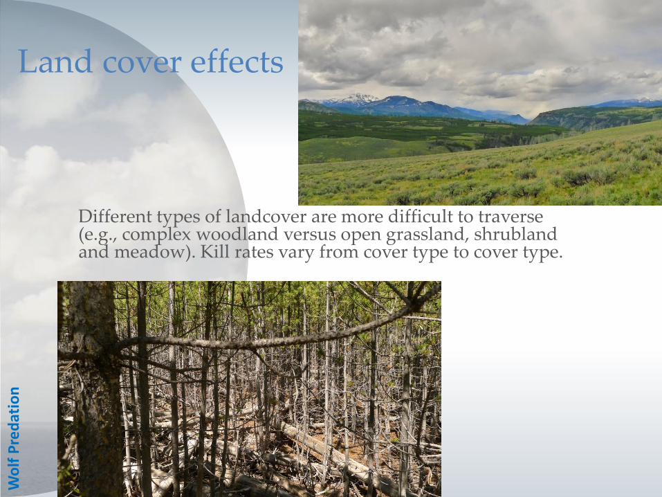
Land cover effects

Different types of landcover are more difficult to traverse (e.g., complex woodland versus open grassland, shrubland and meadow). Kill rates vary from cover type to cover type.

Wo

lf P

red

atio

n

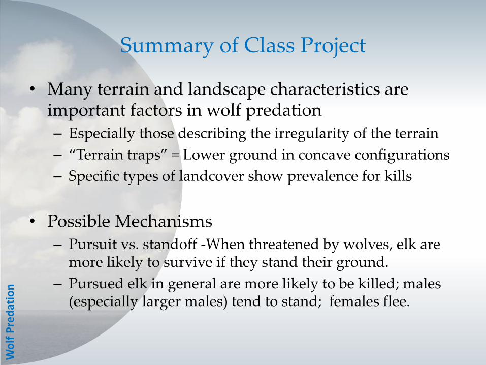
Summary of Class Project

• Many terrain and landscape characteristics are important factors in wolf predation – Especially those describing the irregularity of the terrain

– “Terrain traps” = Lower ground in concave configurations

– Specific types of landcover show prevalence for kills

• Possible Mechanisms – Pursuit vs. standoff -When threatened by wolves, elk are

more likely to survive if they stand their ground.

– Pursued elk in general are more likely to be killed; males (especially larger males) tend to stand; females flee.

Wo

lf P

red

atio

n

Dasymetric Refinement of Boulder Census Demography:

Case Study for Small Area Estimation

Johannes Uhl, MA student

Dept Geography, U. Colorado – Boulder and Dept Geoinformatics, Karlsruhe University, Germany

Context – purpose of the NSF project

Census 2000 summary files for tract, block group, block. Summary files carry fewer attributes than PUMA microdata. Values mostly averages or medians. Microdata carries many more attributes for individual households, but records carry no location info beyond a PUMA code. NSF project working to integrate the microdata estimates with summary files to increase the accessibility of census attributes and to improve reliability of summary file data.

Study area: Two PUMAs surrounding Boulder / Longmont (PUMAs contain ~ 25 census tracts apiece)

Ce

nsu

s R

efin

em

en

t

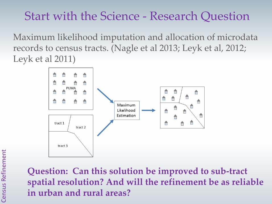
Maximum likelihood imputation and allocation of microdata records to census tracts. (Nagle et al 2013; Leyk et al, 2012; Leyk et al 2011)

Start with the Science - Research Question

Question: Can this solution be improved to sub-tract spatial resolution? And will the refinement be as reliable in urban and rural areas?

Ce

nsu

s R

efin

em

en

t

Dasymetric modeling: Refine enumeration areas to sub-tract-level based on ancillary (limiting) variables.

Dasymetric Modeling

PUMS-based refined tract summaries

GIS Method: Dasymetric Modeling

Clip parts of tracts which are not residential

Recompute densities for revised area

Start with enumerated census population density

Ce

nsu

s R

efin

em

en

t

GIS Workflow

Urban areas:

NLCD Land Use Classes

NLCD Classes 21 + 22

Residential areas

Rural areas:

NLCD Land Use Classes

NLCD Classes 21 + 22

TIGER/Line Roads

Census Block Boundaries

Line Density Raster in 500m

window

Threshold (extract areas where roads/block

boundaries cover >12% of focal window)

Merge Residential

areas

Ce

nsu

s R

efin

em

en

t

Limiting Variable 1 -- Landcover Data

- NLCD Land cover data 2001

Ce

nsu

s R

efin

em

en

t

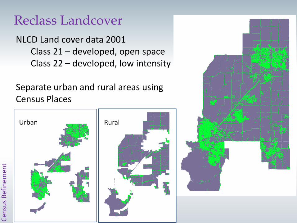
Reclass Landcover

NLCD Land cover data 2001 Class 21 – developed, open space Class 22 – developed, low intensity

Separate urban and rural areas using Census Places

Urban Rural

Ce

nsu

s R

efin

em

en

t

Rural Areas – Extract residential areas using density of roads and census block boundaries

TIGER/Line roads Census Block Boundaries

Limiting variables 2 and 3 (rural areas)

Assumption: - Clusters of local roads indicate residential areas. - Higher density census block boundaries indicates residential areas.

Density grid Extract areas of high density

Ce

nsu

s R

efin

em

en

t

Validation Using Boulder Parcel Data

Residential parcels (source: Boulder County)

Extracted residential areas • NLCD classes 21/22

(urban/rural) • TIGER road density • Census block

boundary density

Dasymetric configuration gives good results but size of residential areas tends to be overestimated, especially in rural areas; implies a need for modifying the density selection of roads and block boundaries C

en

sus

Ref

ine

me

nt

Validation Method

Validation: % pixels of extracted residential areas that: Category 1: contain or intersect residential parcels (Matches) Category 2: are identified as residential parcels but should not be. (Commission Errors = false positives) Category 3: are not identified as residential parcels but should be. (Omission Errors = false negatives) Category 4: are correctly identified as non-residential (Matches)

Cat. 1 Cat. 2 Cat 1+2

Cat. 3 Cat. 4 Cat 3+4

Cat 1+3 Cat 2+4 Total

Residential Parcel

Extracted residential area

Confusion matrix green = correct;

red= error

Ce

nsu

s R

efin

em

en

t

Validation Results - Confusion Matrices

34.36 1.34 35.70

1.93 62.37 64.30

36.29 63.71 100.00

28.16 1.16 29.32

1.72 68.95 70.68

29.88 70.12 100.00

45.67 1.68 47.34

2.31 50.35 52.66

47.97 52.03 100.00

Positive Match

Commission (false pos)

Row 1 Sum

Omission false neg)

Negative Match

Row 2 Sum

Col 1 Sum Col 2 Sum Matrix Total

urban + rural:

rural:

urban:

Normalized by the total area of residential parcels.

Kappa NMI 0.93 0.80 0.93 0.79 0.92 0.76

Ce

nsu

s R

efin

em

en

t

Comparing Small Area Estimates

Initial (Summary File) Estimates Dasymetric Refined Estimates Ce

nsu

s R

efin

em

en

t

Summary of Masters Project

• Dasymetric refinement of tract summaries works – Error rates vary slightly b/t urban and rural areas

– It’s likely that overall success varies too among other urban geographies (e.g., larger more diverse towns, differing geographic constraints)

• How is Johannes’ work being used on the grant? – Working on maximum likelihood imputation that brings in

additional variables (recall that microdata has more attributes than census summary files)

– Testing validation with building footprint vs. parcels (in rural areas, parcels are much larger than actual residential use – harder to access this type of data in US

Wo

lf P

red

atio

n

Conclusion

Exploring our world requires tools that are flexible and powerful.

GIS modeling provides one example of such tools.

• Advantages

– makes it possible to elicit patterns in space and (more recently) time

– adapts to questions about natural or human environmental systems

• Disadvantages

– Capabilities for handling time are limited (display is ok)

– Loose coupling with statistical packages (improving)

Conclusion

Exploring our world requires tools that are flexible and powerful.

GIS modeling relies heavily upon several factors:

• Best results integrate other geospatial tools (remote sensing, GPS)

• GIS Modeling often requires a LOT of data, preprocessed

• Requires computational skills (programming and statistics)

• Interdisciplinary focus is usually beneficial to answering the question.