GIS-ITS Application for Integrated Corridor Management

Transportation leadership you can trust.

presented to

GIS-T 2008

presented byYushuang Zhou and Vassili AlexiadisCambridge Systematics, Inc.

March 2008

1

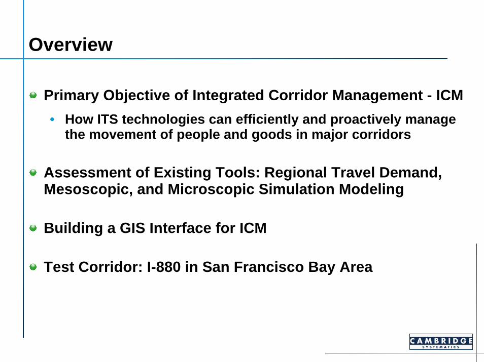
Overview

Primary Objective of Integrated Corridor Management - ICM• How ITS technologies can efficiently and proactively manage

the movement of people and goods in major corridors

Assessment of Existing Tools: Regional Travel Demand, Mesoscopic, and Microscopic Simulation Modeling

Building a GIS Interface for ICM

Test Corridor: I-880 in San Francisco Bay Area

2

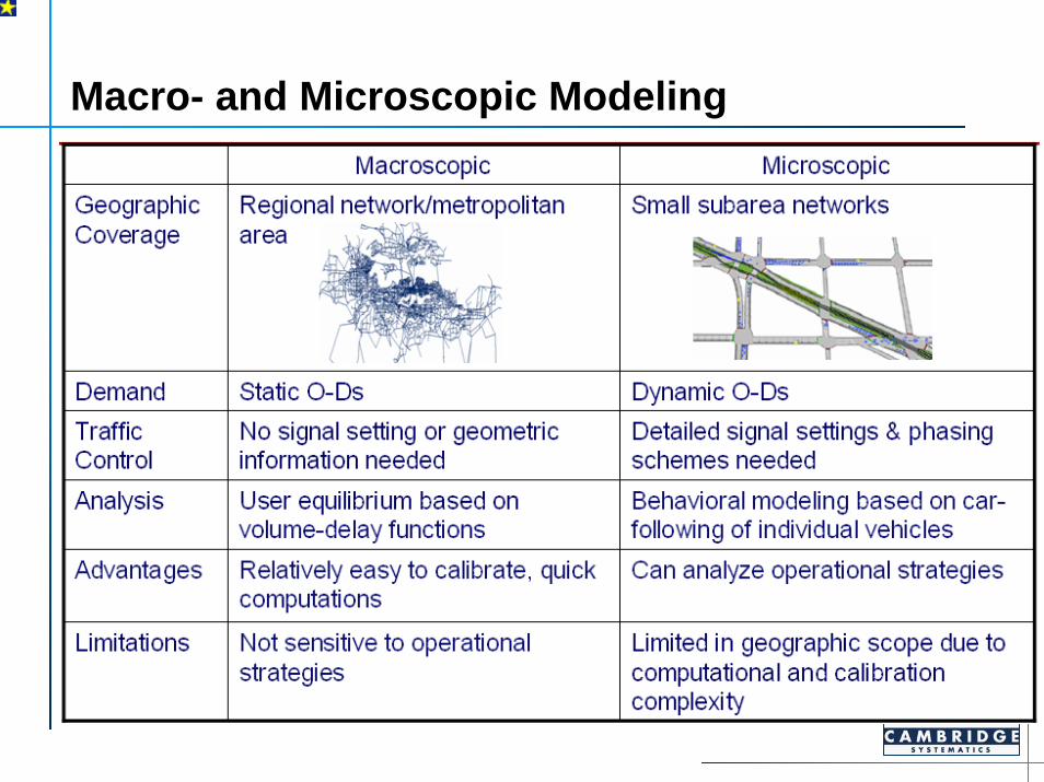
Macroscopic Travel Demand Modeling

Forecast Regional Travel Demand – Highway and Transit

Trip generation, distribution, mode choice and assignments

Not designed to evaluate ITS strategies; Limitedcapabilities to accurately estimate changes in operational characteristics (such as speed, delay, and queuing)

Poor representation of the dynamic nature of traffic

Examples – TransCAD, EMME/2, CUBE

3

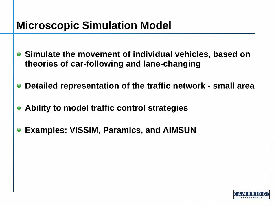
Microscopic Simulation Model

Simulate the movement of individual vehicles, based on theories of car-following and lane-changing

Detailed representation of the traffic network - small area

Ability to model traffic control strategies

Examples: VISSIM, Paramics, and AIMSUN

4

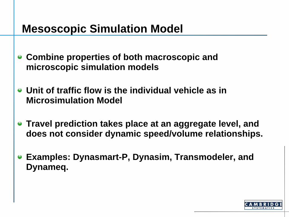
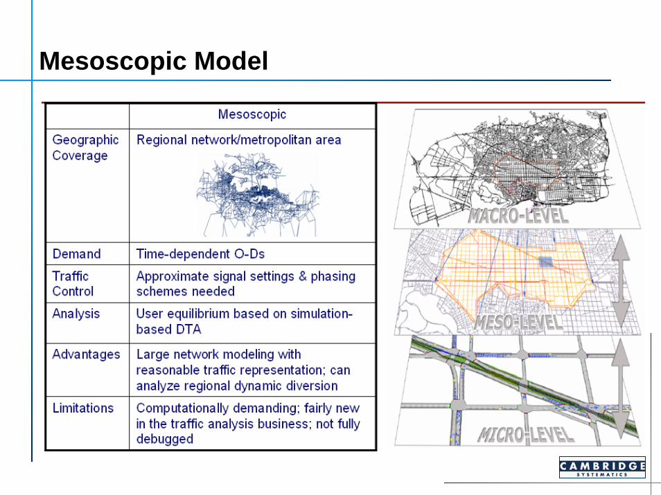
Mesoscopic Simulation Model

Combine properties of both macroscopic and microscopic simulation models

Unit of traffic flow is the individual vehicle as in Microsimulation Model

Travel prediction takes place at an aggregate level, and does not consider dynamic speed/volume relationships.

Examples: Dynasmart-P, Dynasim, Transmodeler, and Dynameq.

5

Macro- and Microscopic Modeling

6

Mesoscopic Model

7

Implementation Options Option 1- Chained by not Integrated

Conventional Approach• Demand model estimates peak period OD table for base

year• OD estimation process used in microsimulation model to

adjust base year OD table to match traffic counts• Base year calibration adjustments carried forward and

applied to all future OD tables produced by the demand model

• Apply capacity constraint

Practical limitations on OD adjustment• Labor intensive• Ad-hoc nature of OD adjustments

8

Implementation OptionsOption 2 – Fully Integrated

Several recent software implementations• Cube/Dynasim (Avenue)• EMME3/Dynameq• TransCad/TransModeler• Visum/Vissim• AIMSUN• …

Limited application experience

9

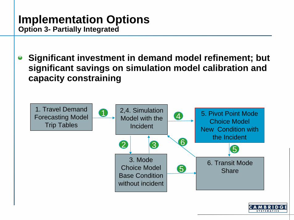
Implementation Options Option 3- Partially Integrated

Significant investment in demand model refinement; but significant savings on simulation model calibration and capacity constraining

1. Travel Demand Forecasting Model

Trip Tables

2,4. Simulation Model with the

Incident

3. Mode Choice Model

Base Condition without incident

5. Pivot Point Mode Choice Model

New Condition with the Incident

6. Transit Mode Share

1

2 3

4

5

5

6

10

Calculate Mode Shift

Drive-Alone50% Mode Share

Local Bus20% Mode Share

Light Rail30% Mode ShareOrigin Dest.

Mode ShareAnalysis

Drive-AloneTravel Time: 45 minWalk Time: 0 minTransfers: 0

Local BusTravel Time: 60 minWalk Time: 10 minTransfers: 1

Light RailTravel Time: 35 minWalk Time: 20 minTransfers: 0

Origin Dest.

Levels of Service

Origin Dest.

Service Network

Local Bus Local Bus

Light Rail

Drive-Alone

A

B

11

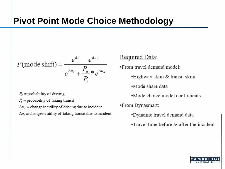
Pivot Point Mode Choice Methodology

12

Study Area

Segment 1: OaklandUrban Area, 12.2 mi

Segment II: Hayward/FremontUrban/light industrial Area, 15.2 mi

Segment III: Fremont/MilpitasSurburban Area, 5.3 miles

• Residential, commercial and industrial uses

• Port, international, Airport, Sports Arena

• Approximately 35 miles

• Heavy daily traffic –Freeway AADT (120,000 - 275,000)

• HOV lane, arterials, bus/rail transit

• Automated data archival for freeways

13

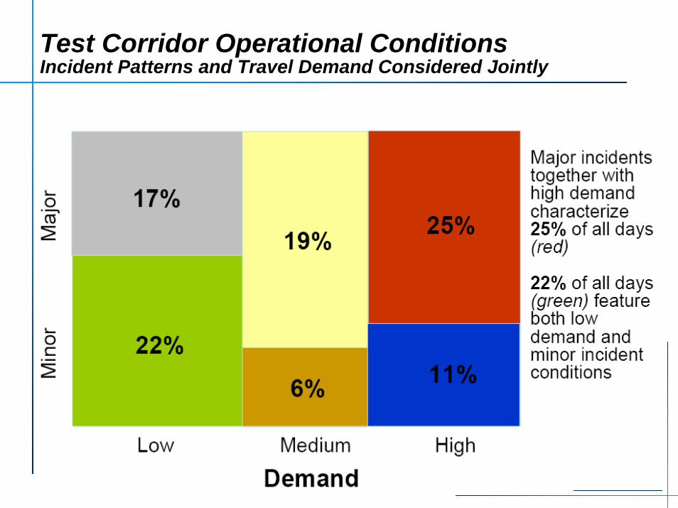
Test Corridor Operational ConditionsIncident Patterns and Travel Demand Considered Jointly

14

Incident Condition

•North bound•7:15AM, Wkday•2 lanes blocked•duration 45 min

15

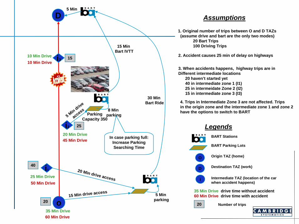
o

D

15 Min drive access

30 Min Bart Ride

5 Min parking

5 Min

35 Min Drive

25 Min Drive

20 Min Drive

10 Min Drive

i1

i2

i3

20

40

25

15

20 Min drive access

5 Min drive

access 8 Min parking

15 Min Bart IVTT

ParkingCapacity 350

In case parking full: Increase Parking Searching Time

50 Min Drive

60 Min Drive

45 Min Drive

10 Min Drive2. Accident causes 25 min of delay on highways

3. When accidents happens, highway trips are in Different intermediate locations

20 haven’t started yet 40 in intermediate zone 1 (I1)25 in intermeidate Zone 2 (I2)15 in intermediate zone 3 (I3)

4. Trips in Intermediate Zone 3 are not affected. Trips in the origin zone and the intermediate zone 1 and zone 2 have the options to switch to BART

1. Original number of trips between O and D TAZs (assume drive and bart are the only two modes)

20 Bart Trips100 Driving Trips

Assumptions

BART Parking Lots

BART Stations

O Origin TAZ (home)

D Destination TAZ (work)

i Intermediate TAZ (location of the car when accident happens)

35 Min Drive drive time without accident60 Min Drive drive time with accident

20 Number of trips

Legends

16

User Interface for Data InputGIS layers and travel demand modelSpecify Mode Choice Model Input

17

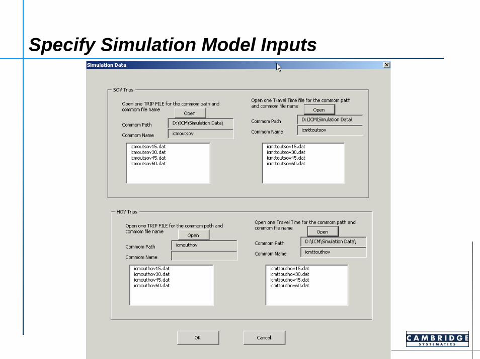
User Interface for Data Input from simulation model (trip and travel time)Specify Simulation Model Inputs

18

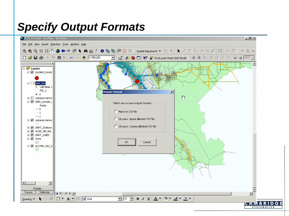
Specify Output FormatSpecify Output Formats

19

Scenarios Being Tested

20

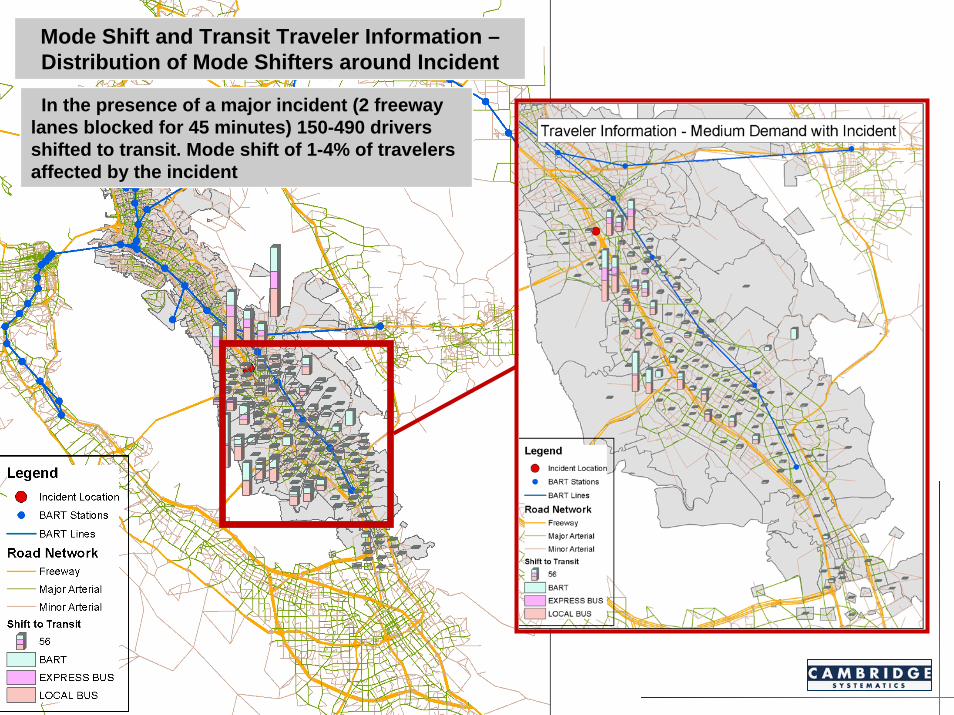
Mode Shift and Transit Traveler Information –Distribution of Mode Shifters around Incident

In the presence of a major incident (2 freeway lanes blocked for 45 minutes) 150-490 drivers shifted to transit. Mode shift of 1-4% of travelers affected by the incident

21

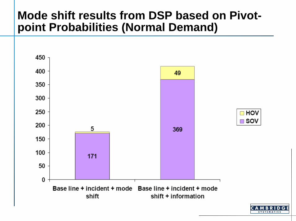
Mode shift results from DSP based on Pivot-point Probabilities (Normal Demand)

22

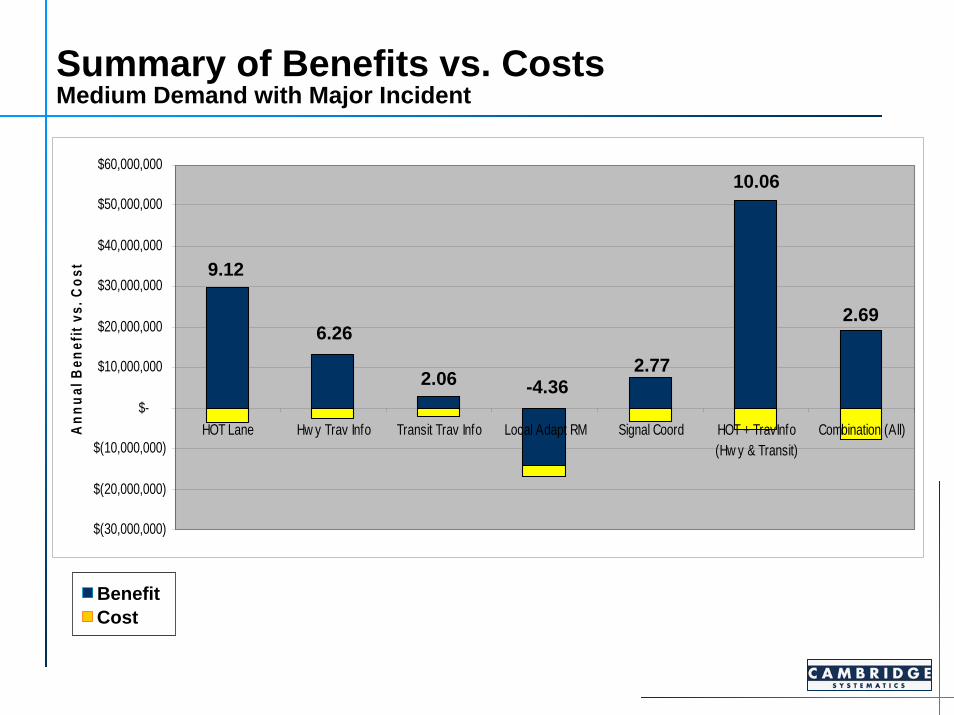
Summary of Benefits vs. CostsMedium Demand with Major Incident

$(30,000,000)

$(20,000,000)

$(10,000,000)

$-

$10,000,000

$20,000,000

$30,000,000

$40,000,000

$50,000,000

$60,000,000

HOT Lane Hw y Trav Info Transit Trav Info Local Adapt RM Signal Coord HOT + TravInfo(Hw y & Transit)

Combination (All)Ann

ual B

enef

it vs

. Cos

t 9.12

6.26

2.06 -4.362.77

10.06

2.69

BenefitCost

23

Effectiveness of Strategies Under Different Operational Regimes (B-C)

Questions and Answers