Getting Started with Microsoft Excel This handout provides an introduction to Microsoft Excel, a popular spreadsheet application installed on PCs and Macs in the Student Microcomputer Facility. The document covers the Excel interface, opening and saving worksheets, entering and editing data, building formulas and functions, formatting, and printing your data.

Starting Excel

You can start Excel by:

1. Double-clicking on the Microsoft Excel application icon. This application is usually in a folder called Excel. An alias for this icon appears on the desktop of the computers in the Student Microcomputer Facility.

. Double-clicking on the icon of any Excel document. When you double-click an Excel document, Excel opens with the document already loaded.

Exploring the Excel Interface

Components of the Excel Window

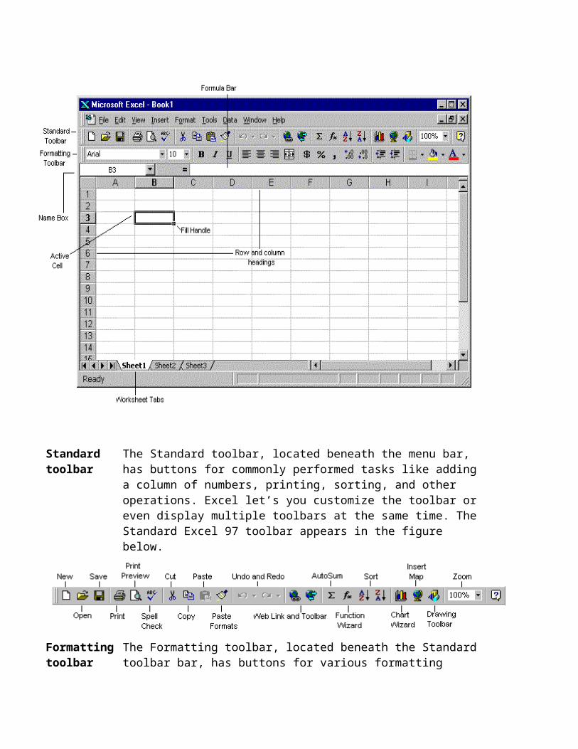
Besides the usual window components (close box, title bar, scroll bars, etc.), an Excel window has several unique elements identified in the figure at the top of the next page.

Mail Merge Popularity: Download Buy NowMail Merge for Excel provides a simple facility to run a mail merge entirely in Microsoft Excel software in a similar fashion to the facility provided in Microsoft Word software.

This may be useful for mail merging forms or data with other complex formulas or look ups. It may also be quicker and easier for those who have little or no experience with Microsoft Word but are familiar with Microsoft Excel.

Mail Merge for Excel is simple and intuitive to use. There is a full help file and an example file to see, both provided with the software.

The results of the Mail Merge can be output to: A print preview for testing (or individual selection to print), A printer, A file - either one text file (.txt) with page breaks between or individual text files, To individual Microsoft Excel workbooks or HTML (not Microsoft Excel 97) files, or Direct to individual emails with text file attachments (Microsoft Excel workbook attachments or plain text

in the body).

To run a mail merge with Mail Merge for Excel you simply create two worksheets. The first (main document) contains your form, letter, etc, with the merge fields included in cells marked with << >> (eg cell A6 might contain "Dear <>,"). The sheet can be named as you wish, and can contain any number of merge fields anywhere on it alongside any other look ups, formulas etc. The second sheet will contain the source data. In row 1 you put the merge field names (without the << >>), and below you have your data to be merged

Standard toolbar

The Standard toolbar, located beneath the menu bar, has buttons for commonly performed tasks like adding a column of numbers, printing, sorting, and other operations. Excel let’s you customize the toolbar or even display multiple toolbars at the same time. The Standard Excel 97 toolbar appears in the figure below.

Formatting toolbar

The Formatting toolbar, located beneath the Standard toolbar bar, has buttons for various formatting operations like changing text size or style, formatting numbers and placing borders around cells.

Formula bar The formula bar is located beneath the toolbar at the top of the Excel worksheet. Use the formula bar to enter and edit worksheet data. The contents of the active cell always appear in the formula bar. When you click the mouse in the formula bar, an X and a check mark appear. You can click the check icon to confirm and completes editing, or the X to abandon editing.

Name box The Name box displays the reference of the selected cells.

Row and column headings

Letters and numbers identify the rows and columns on an Excel spreadsheet. The intersection of a row and a column is called a cell. Use row and column headings to specify a cell's reference. For example, the cell located where column B and row 7 intersect is called B7.

Active cell The active cell has a dark border around it to indicate your position in the worksheet. All text and numbers that you type are inserted into the active cell. Click the mouse on a cell to make it active.

Fill handle The lower right corner of the active cell has a small box called a Fill Handle. Your mouse changes to a cross-hair when you are on the Fill Handle. The Fill Handle helps you copy data and create series of information. For example, if you type January in the active cell and then drag the Fill Handle over four cells, Excel automatically inserts February, March, April and May.

Worksheet tabs

An Excel workbook consists of multiple worksheets. Use the worksheet tabs at the bottom of the screen to navigate between worksheets within a workbook.

 

Entering and Editing Data

Entering Data

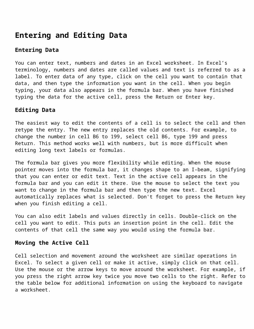
You can enter text, numbers and dates in an Excel worksheet. In Excel’s terminology, numbers and dates are called values and text is referred to as a label. To enter data of any type, click on the cell you want to contain that data, and

then type the information you want in the cell. When you begin typing, your data also appears in the formula bar. When you have finished typing the data for the active cell, press the Return or Enter key.

Editing Data

The easiest way to edit the contents of a cell is to select the cell and then retype the entry. The new entry replaces the old contents. For example, to change the number in cell B6 to 199, select cell B6, type 199 and press Return. This method works well with numbers, but is more difficult when editing long text labels or formulas.

The formula bar gives you more flexibility while editing. When the mouse pointer moves into the formula bar, it changes shape to an I-beam, signifying that you can enter or edit text. Text in the active cell appears in the formula bar and you can edit it there. Use the mouse to select the text you want to change in the formula bar and then type the new text. Excel automatically replaces what is selected. Don't forget to press the Return key when you finish editing a cell.

You can also edit labels and values directly in cells. Double-click on the cell you want to edit. This puts an insertion point in the cell. Edit the contents of that cell the same way you would using the formula bar.

Moving the Active Cell

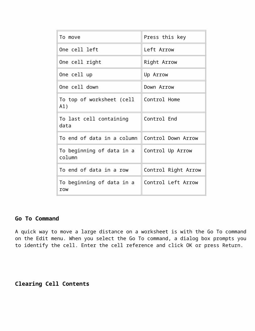
Cell selection and movement around the worksheet are similar operations in Excel. To select a given cell or make it active, simply click on that cell. Use the mouse or the arrow keys to move around the worksheet. For example, if you press the right arrow key twice you move two cells to the right. Refer to the table below for additional information on using the keyboard to navigate a worksheet.

To move Press this key

One cell left Left Arrow

One cell right Right Arrow

One cell up Up Arrow

One cell down Down Arrow

To top of worksheet (cell A1) Control Home

To last cell containing data Control End

To end of data in a column Control Down Arrow

To beginning of data in a column Control Up Arrow

To end of data in a row Control Right Arrow

To beginning of data in a row Control Left Arrow

 

Go To Command

A quick way to move a large distance on a worksheet is with the Go To command on the Edit menu. When you select the Go To command, a dialog box prompts you to identify the cell. Enter the cell reference and click OK or press Return.

Clearing Cell Contents

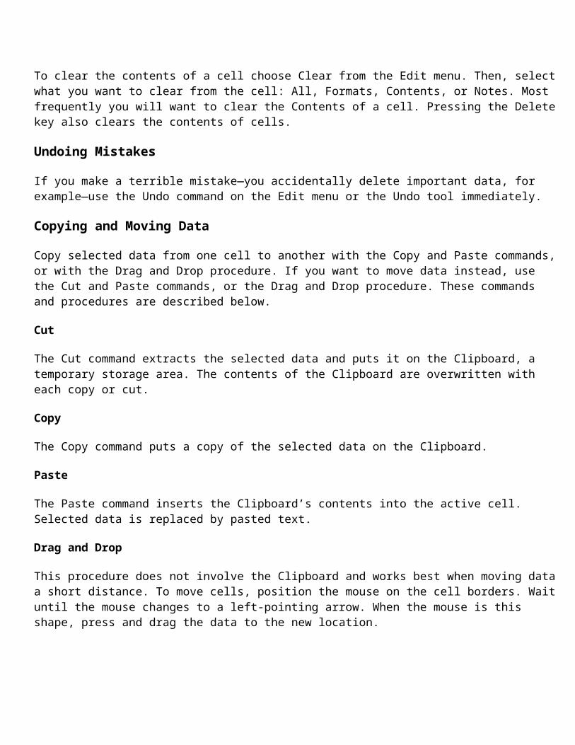
To clear the contents of a cell choose Clear from the Edit menu. Then, select what you want to clear from the cell: All, Formats, Contents, or Notes. Most frequently you will want to clear the Contents of a cell. Pressing the Delete key also clears the contents of cells.

Undoing Mistakes

If you make a terrible mistake—you accidentally delete important data, for example—use the Undo command on the Edit menu or the Undo tool immediately.

Copying and Moving Data

Copy selected data from one cell to another with the Copy and Paste commands, or with the Drag and Drop procedure. If you want to move data instead, use the Cut and Paste commands, or the Drag and Drop procedure. These commands and procedures are described below.

Cut

The Cut command extracts the selected data and puts it on the Clipboard, a temporary storage area. The contents of the Clipboard are overwritten with each copy or cut.

Copy

The Copy command puts a copy of the selected data on the Clipboard.

Paste

The Paste command inserts the Clipboard’s contents into the active cell. Selected data is replaced by pasted text.

Drag and Drop

This procedure does not involve the Clipboard and works best when moving data a short distance. To move cells, position the mouse on the cell borders. Wait until the mouse changes to a left-pointing arrow. When the mouse is this shape, press and drag the data to the new location.

Working with Excel documents

Opening and Closing Documents

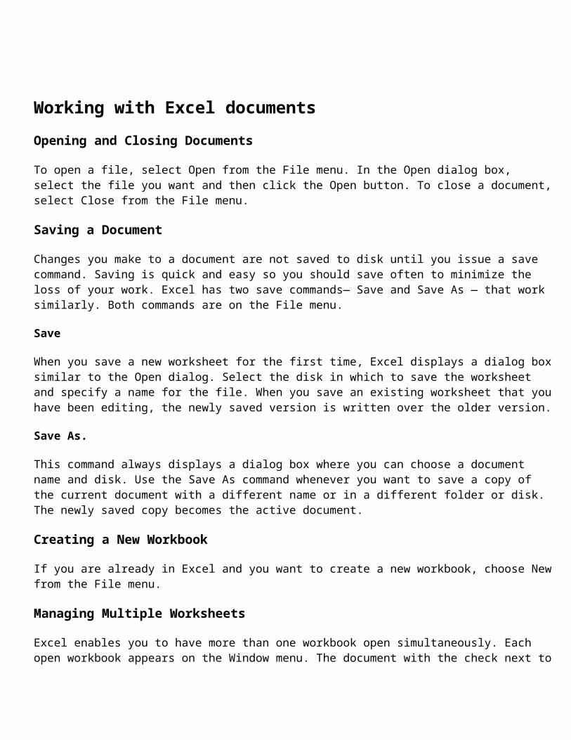
To open a file, select Open from the File menu. In the Open dialog box, select the file you want and then click the Open button. To close a document, select Close from the File menu.

Saving a Document

Changes you make to a document are not saved to disk until you issue a save command. Saving is quick and easy so you should save often to minimize the loss of your work. Excel has two save commands— Save and Save As — that work similarly. Both commands are on the File menu.

Save

When you save a new worksheet for the first time, Excel displays a dialog box similar to the Open dialog. Select the disk in which to save the worksheet and specify a name for the file. When you save an existing worksheet that you have been editing, the newly saved version is written over the older version.

Save As.

This command always displays a dialog box where you can choose a document name and disk. Use the Save As command whenever you want to save a copy of the current document with a different name or in a different folder or disk. The newly saved copy becomes the active document.

Creating a New Workbook

If you are already in Excel and you want to create a new workbook, choose New from the File menu.

Managing Multiple Worksheets

Excel enables you to have more than one workbook open simultaneously. Each open workbook appears on the Window menu. The document with the check next to it is the active document. To switch to another document, simply choose that document from the Window menu.

To navigate between worksheets within a workbook, click the worksheet tab you want to activate. Double-click a worksheet tab to change its name.

Getting Help

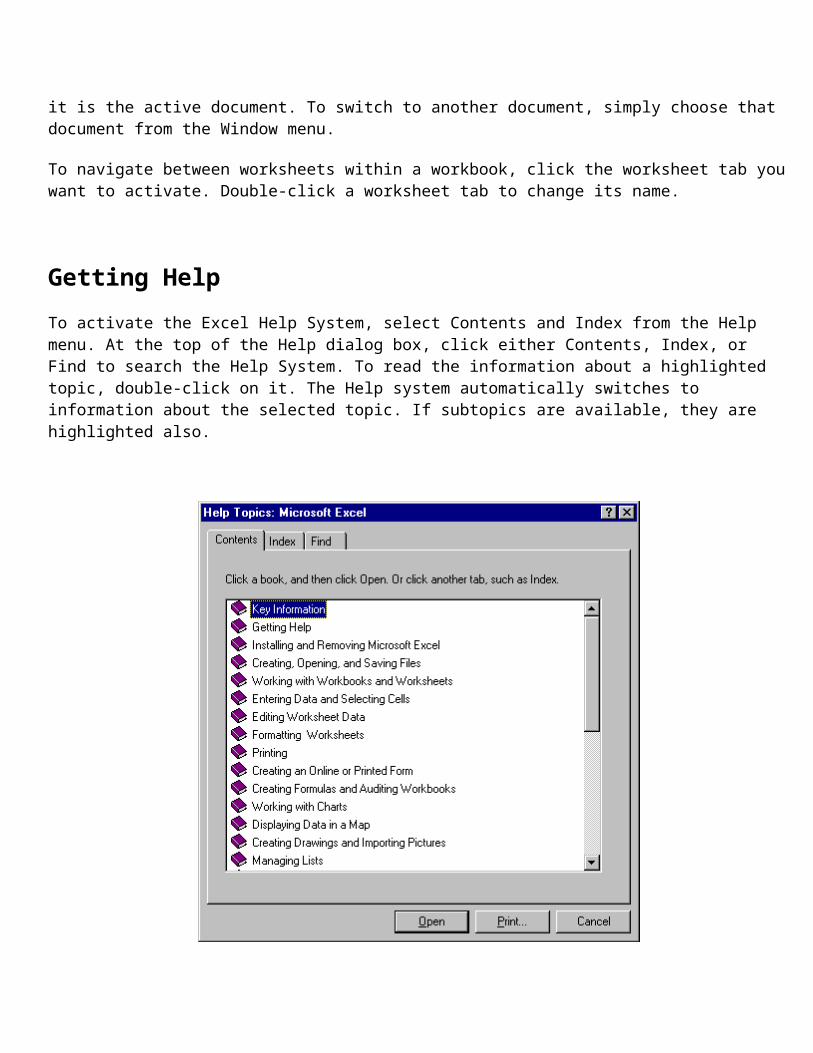
To activate the Excel Help System, select Contents and Index from the Help menu. At the top of the Help dialog box, click either Contents, Index, or Find to search the Help System. To read the information about a highlighted topic, double-click on it. The Help system automatically switches to information about the selected topic. If subtopics are available, they are highlighted also.

 

 

Help on the Web

Choose Microsoft on the Web from the Help menu to find additional help, FAQs, and free downloads for Microsoft Excel.

Formulas and Functions

Formulas and functions that perform calculations are the true power of spreadsheets. This section describes how to construct formulas and functions on an Excel worksheet.

Formulas

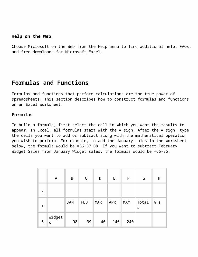
To build a formula, first select the cell in which you want the results to appear. In Excel, all formulas start with the = sign. After the = sign, type the cells you want to add or subtract along with the mathematical operation you wish to perform. For example, to add the January sales in the worksheet below, the formula would be =B6+B7+B8. If you want to subtract February Widget Sales from January Widget sales, the formula would be =C6-B6.

 

 A B C D E F G H

4               

5  JAN FEB MAR APR MAY Totals %'s

6Widgets

98 39 40 140 240   

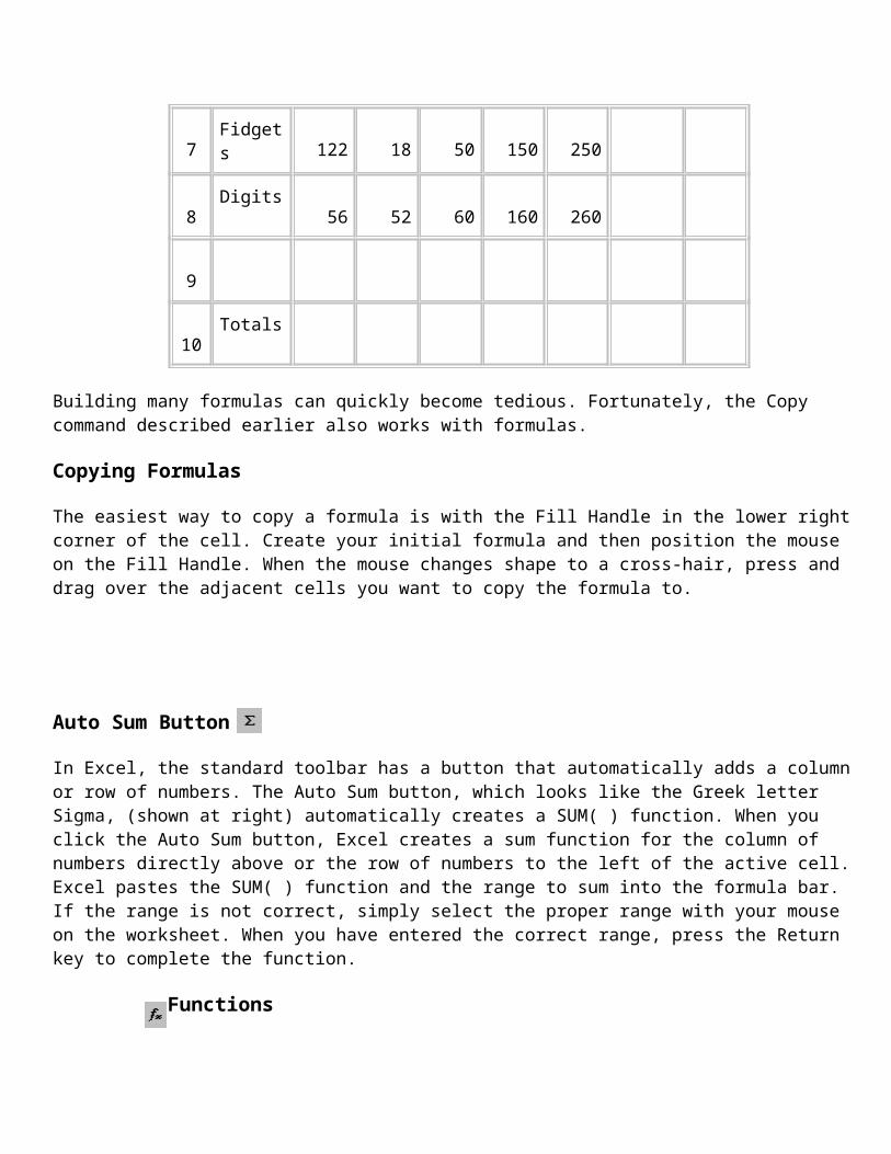
7Fidgets

122 18 50 150 250   

8Digits

56 52 60 160 260   

9               

10Totals              

Building many formulas can quickly become tedious. Fortunately, the Copy command described earlier also works with formulas.

Copying Formulas

The easiest way to copy a formula is with the Fill Handle in the lower right corner of the cell. Create your initial formula and then position the mouse on the Fill Handle. When the mouse changes shape to a cross-hair, press and drag over the adjacent cells you want to copy the formula to.

Auto Sum Button

In Excel, the standard toolbar has a button that automatically adds a column or row of numbers. The Auto Sum button, which looks like the Greek letter Sigma, (shown at right) automatically creates a SUM( ) function. When you click the Auto Sum button, Excel creates a sum function for the column of numbers directly above or the row of numbers to the left of the active cell. Excel pastes the SUM( ) function and the range to sum into the formula bar. If the range is not correct, simply select the proper range with your mouse on the worksheet. When you have entered the correct range, press the Return key to complete the function.

Functions

As you saw above, formulas can be very useful on a worksheet. However, what if you want to add up a column of 10 numbers? Do you have to click on ten cells or type ten cell references in a formula? Excel has a more efficient means of dealing with this situation by using functions.

The SUM( ) function is probably the most common function in Excel. It adds a range of numbers. To build a SUM( ) function, begin by typing =SUM(. Next, tell Excel which cells to sum. Using the mouse, press and drag over the range of cells you wish to add. A dotted outline appears around the cells, and Excel displays the cell range in the formula bar. When you have the correct cells selected, release the mouse button, close the parenthesis, and press the Return key.

If you do not want to use the mouse, type in the cells you want Excel to sum. For example, to sum cells B6 through B8, type =SUM(B6:B8). Excel interprets B6:B8 as the range of cells from B6 to B8.

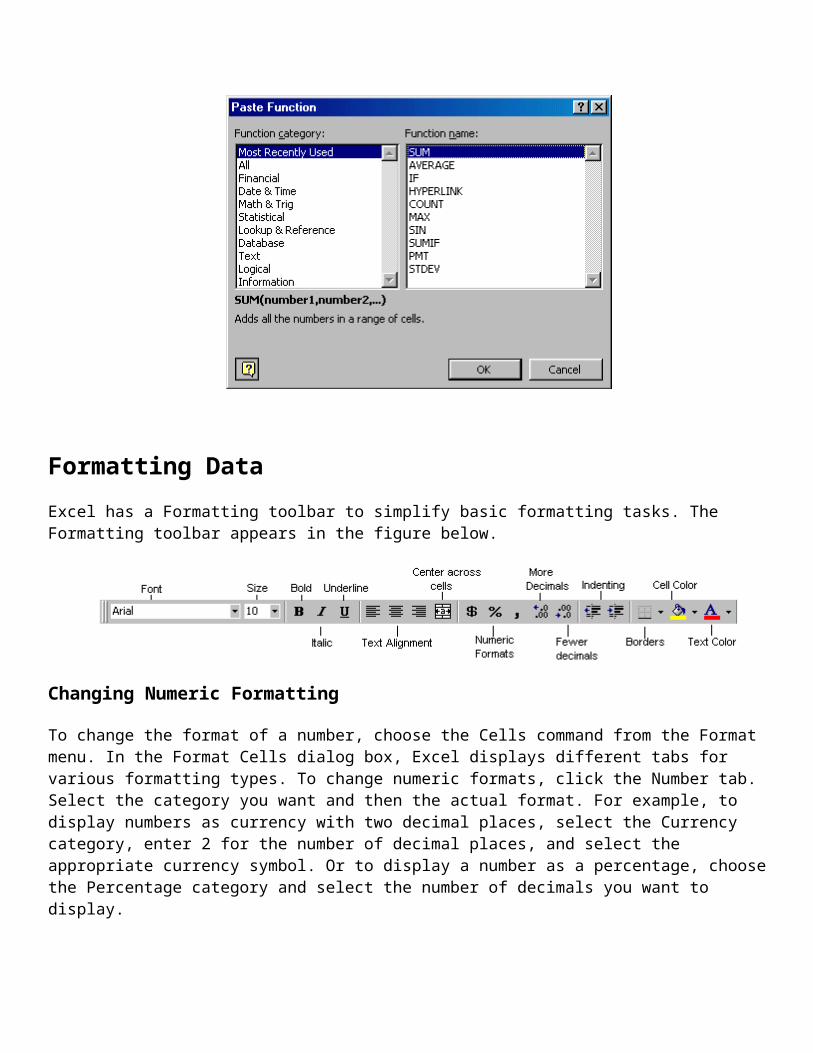
Using the Paste Function tool

Excel has many more functions besides the SUM() function described above. For example, you might want to calculate the average of a column of numbers, or count how many entries are in a row. You can get help with these functions and hundreds more by using Excel’s Paste Function tool.

The Paste Function tool is located on the Standard toolbar. Click the tool (shown at right) to activate the dialog box. First, choose the Function Category you are interested in and then select the function you want in that category. When you have selected the proper function click OK to move to Step 2. In second dialog box, specify the cells the function will operate on, called its arguments. Select the cells with the mouse and click OK. Notice the creation of the function in the formula bar.

 

Formatting Data

Excel has a Formatting toolbar to simplify basic formatting tasks. The Formatting toolbar appears in the figure below.

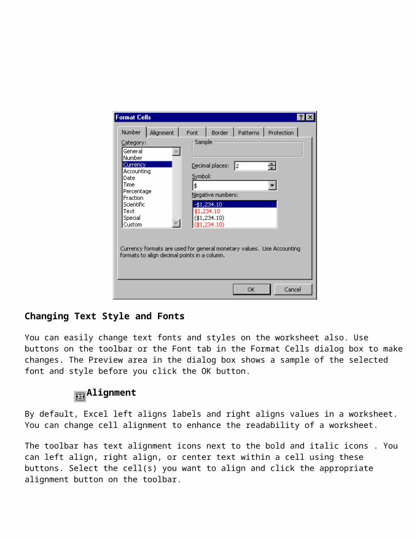
Changing Numeric Formatting

To change the format of a number, choose the Cells command from the Format menu. In the Format Cells dialog box, Excel displays different tabs for various formatting types. To change numeric formats, click the Number tab. Select the category you want and then the actual format. For example, to display numbers as currency with two decimal places, select the Currency category, enter 2 for the number of decimal places, and select the appropriate currency symbol. Or to display a number as a percentage, choose the Percentage category and select the number of decimals you want to display.

Changing Text Style and Fonts

You can easily change text fonts and styles on the worksheet also. Use buttons on the toolbar or the Font tab in the Format Cells dialog box to make changes. The Preview area in the dialog box shows a sample of the selected font and style before you click the OK button.

Alignment

By default, Excel left aligns labels and right aligns values in a worksheet. You can change cell alignment to enhance the readability of a worksheet.

The toolbar has text alignment icons next to the bold and italic icons . You can left align, right align, or center text within a cell using these buttons. Select the cell(s) you want to align and click the appropriate alignment button on the toolbar.

The toolbar also has a button (shown at right) that will center a label over a range of cells, for example centering a title over a report. To center data over a range of cells, select the cell you want to center, and the columns you want to center it over, and click the Center over Cells button.

Placing Borders around Cells

Use the Borders button on the toolbar to place borders around cells. The Border tab in the Format Cells dialog box provides greater flexibility in creating borders.

Changing Column Widths

Change column widths by dragging column borders with the mouse. Move the mouse pointer to the right border of a column heading until the mouse pointer changes shape to a left and right pointing arrow. When the mouse pointer changes shape, click and drag the mouse to adjust the column width. Note that when you are adjusting the width in this way, a numeric width indicator appears in the upper left part of the formula bar.

Page Setup, Previewing and Printing

Before you actually print a worksheet, you should provide Excel information about margins, headers, footers, and page orientation. You change these settings using the Page Setup option on the File menu.

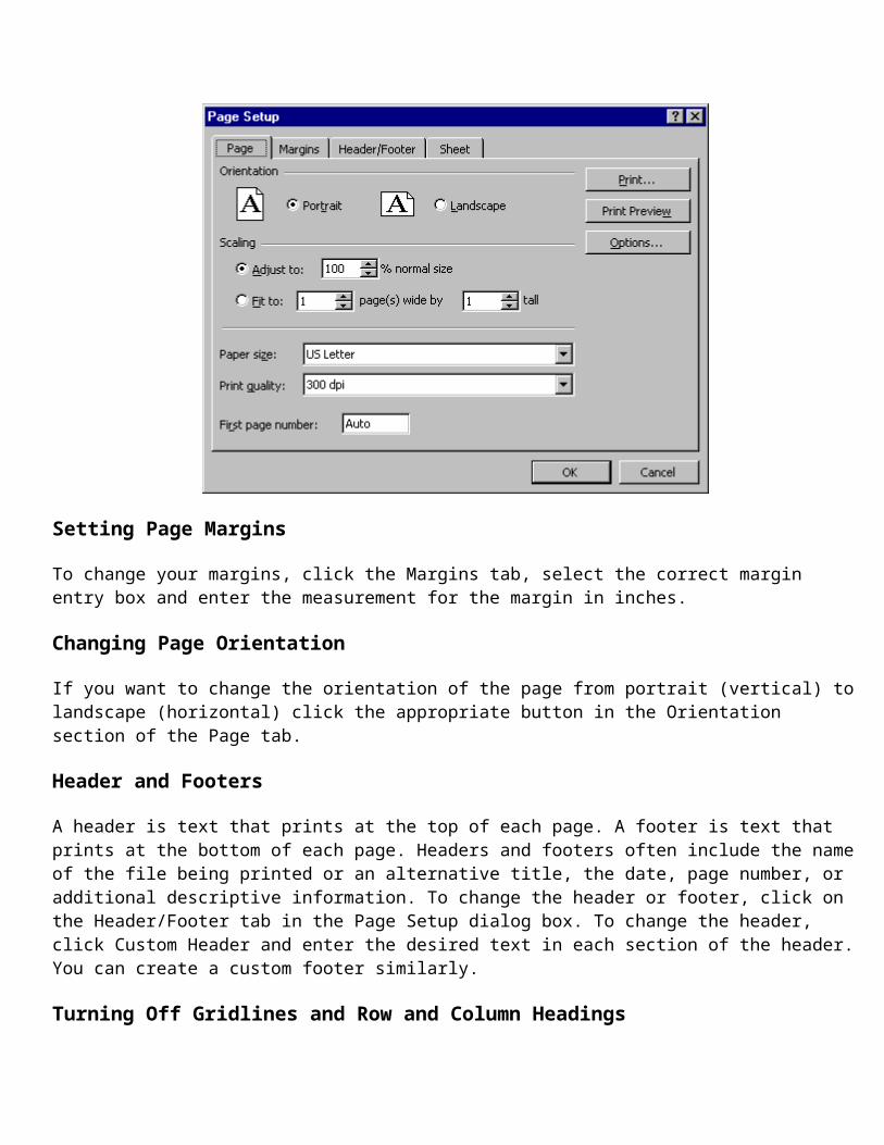
Page Setup

The Page Setup dialog box, shown below, has controls for margins, page orientation, headers and footers and whether gridlines and row and column headings should be printed.

Setting Page Margins

To change your margins, click the Margins tab, select the correct margin entry box and enter the measurement for the margin in inches.

Changing Page Orientation

If you want to change the orientation of the page from portrait (vertical) to landscape (horizontal) click the appropriate button in the Orientation section of the Page tab.

Header and Footers

A header is text that prints at the top of each page. A footer is text that prints at the bottom of each page. Headers and footers often include the name of the file being printed or an alternative title, the date, page number, or additional descriptive information. To change the header or footer, click on the Header/Footer tab in the Page Setup dialog box. To change the header, click Custom Header and enter the desired text in each section of the header. You can create a custom footer similarly.

Turning Off Gridlines and Row and Column Headings

Although row and column headings and gridlines are helpful on the screen, these additions are rarely necessary in printed output and may even detract from it. Choose the Sheet tab and click the check boxes for Row and Column Headings and Gridlines to turn these features off.

Previewing

Before printing, preview your output by selecting Print Preview from the File menu. When in Print Preview, Excel displays how the document will print on the page, but it is difficult to actually read the text. Notice that the mouse pointer takes the shape of a magnifying glass. You can enlarge the printed image by clicking the Zoom button or by using the magnifying glass. Simply click the magnifying glass on a part of the page you want to enlarge.

The Print Preview screen also has several buttons at the top of the screen that enable you to make adjustments. For example, the Setup button opens the Page Setup dialog box and the Margins button lets you change page margins and column widths to fit more information on one page.

If you are satisfied with the appearance of your document in the Print Preview screen, the Print button lets you send your output directly to the printer.

Excel also has Page Break Preview on the View menu that lets you see your page breaks and change them by dragging borders. Choose View and Page Break Preview to display this mode.

Printing

To print your worksheet, choose Print from the File menu, or click the Print button from the Print Preview screen. This displays a dialog box that lets you change print settings and specify the number of copies to print. You should also indicate whether you want to print the active worksheet, the selected cells only, or the whole workbook.

 

Review and Summary

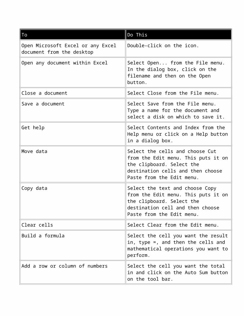
To Do This

Open Microsoft Excel or any Excel document from the desktop

Double-click on the icon.

Open any document within Excel Select Open... from the File menu. In the dialog box, click on the filename and then on the Open button.

Close a document Select Close from the File menu.

Save a document Select Save from the File menu. Type a name for the document and select a disk on which to save it.

Get help Select Contents and Index from the Help menu or click on a Help button in a dialog box.

Move data Select the cells and choose Cut from the Edit menu. This puts it on the clipboard. Select the destination cells and then choose Paste from the Edit menu.

Copy data Select the text and choose Copy from the Edit menu. This puts it on the clipboard. Select the destination cell and then choose Paste from the Edit menu.

Clear cells Select Clear from the Edit menu.

Build a formula Select the cell you want the result in, type =, and then the cells and mathematical operations you want to perform.

Add a row or column of numbers Select the cell you want the total in and click on the Auto Sum button on the tool bar.

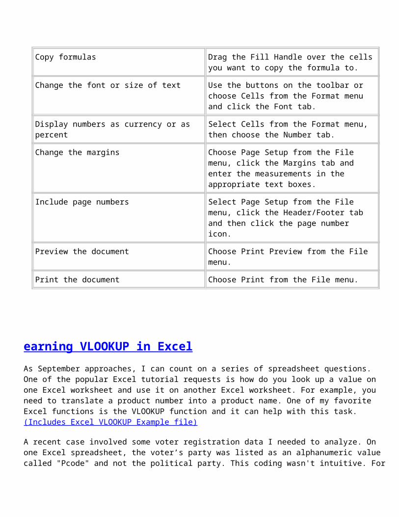
Copy formulas Drag the Fill Handle over the cells you want to copy the formula to.

Change the font or size of text Use the buttons on the toolbar or choose Cells from the Format menu and click the Font tab.

Display numbers as currency or as percent Select Cells from the Format menu, then choose the Number tab.

Change the margins Choose Page Setup from the File menu, click the Margins tab and enter the measurements in the appropriate text boxes.

Include page numbers Select Page Setup from the File menu, click the Header/Footer tab and then click the page number icon.

Preview the document Choose Print Preview from the File menu.

Print the document Choose Print from the File menu.

 

earning VLOOKUP in Excel

As September approaches, I can count on a series of spreadsheet questions. One of the popular Excel tutorial requests is how do you look up a value on one Excel worksheet and use it on another Excel worksheet. For example, you need to translate a product number into a product name. One of my favorite Excel functions is the VLOOKUP function and it can help with this task. (Includes Excel VLOOKUP Example file)

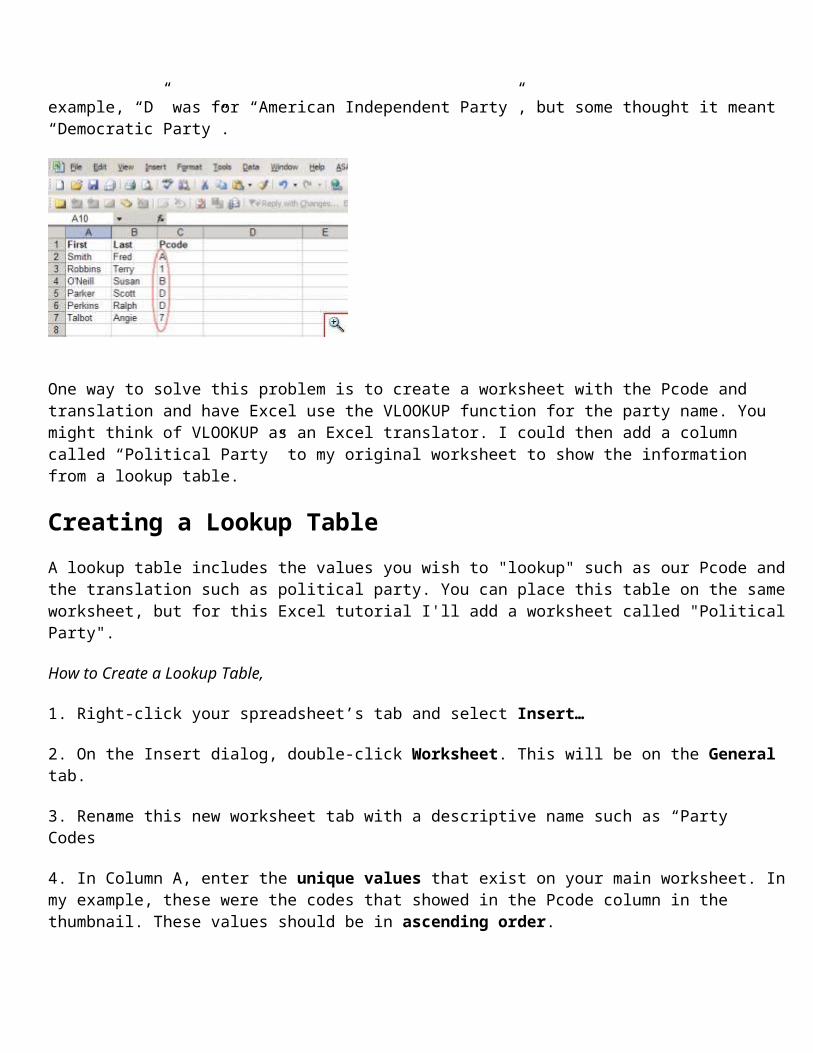
A recent case involved some voter registration data I needed to analyze. On one Excel spreadsheet, the voter’s party was listed as an alphanumeric value called "Pcode" and not the political party. This coding wasn't intuitive. For example, “D” was for “American Independent Party”, but some thought it meant “Democratic Party”.

One way to solve this problem is to create a worksheet with the Pcode and translation and have Excel use the VLOOKUP function for the party name. You might think of VLOOKUP as an Excel translator. I could then add a column called “Political Party” to my original worksheet to show the information from a lookup table.

Creating a Lookup Table

A lookup table includes the values you wish to "lookup" such as our Pcode and the translation such as political party. You can place this table on the same worksheet, but for this Excel tutorial I'll add a worksheet called "Political Party".

How to Create a Lookup Table,

1. Right-click your spreadsheet’s tab and select Insert…

2. On the Insert dialog, double-click Worksheet. This will be on the General tab.

3. Rename this new worksheet tab with a descriptive name such as “Party Codes”

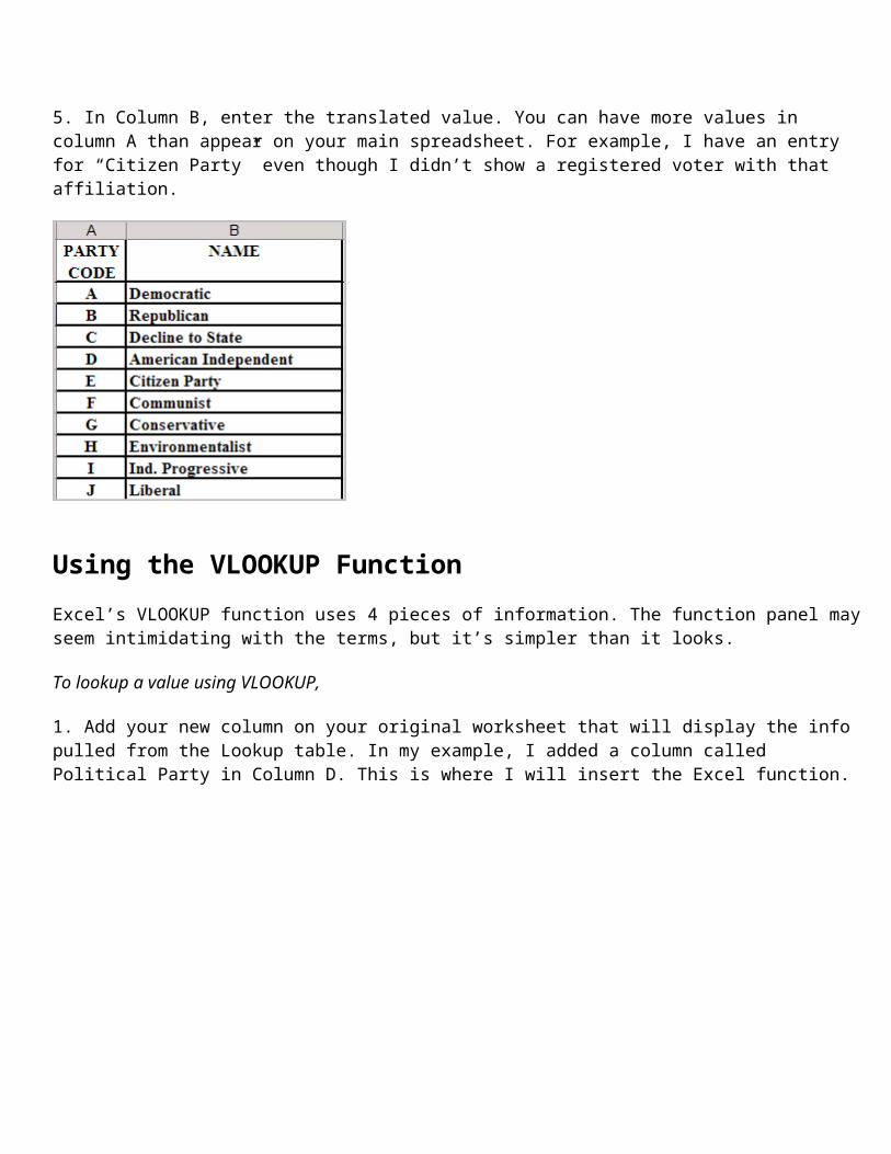
4. In Column A, enter the unique values that exist on your main worksheet. In my example, these were the codes that showed in the Pcode column in the thumbnail. These values should be in ascending order.

5. In Column B, enter the translated value. You can have more values in column A than appear on your main spreadsheet. For example, I have an entry for “Citizen Party” even though I didn’t show a registered voter with that affiliation.

Using the VLOOKUP Function

Excel’s VLOOKUP function uses 4 pieces of information. The function panel may seem intimidating with the terms, but it’s simpler than it looks.

To lookup a value using VLOOKUP,

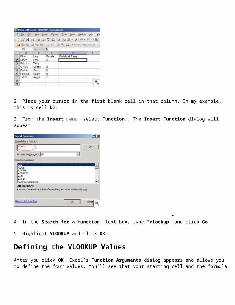
1. Add your new column on your original worksheet that will display the info pulled from the Lookup table. In my example, I added a column called Political Party in Column D. This is where I will insert the Excel function.

2. Place your cursor in the first blank cell in that column. In my example, this is cell D2.

3. From the Insert menu, select Function…. The Insert Function dialog will appear.

4. In the Search for a function: text box, type “vlookup” and click Go.

5. Highlight VLOOKUP and click OK.

Defining the VLOOKUP Values

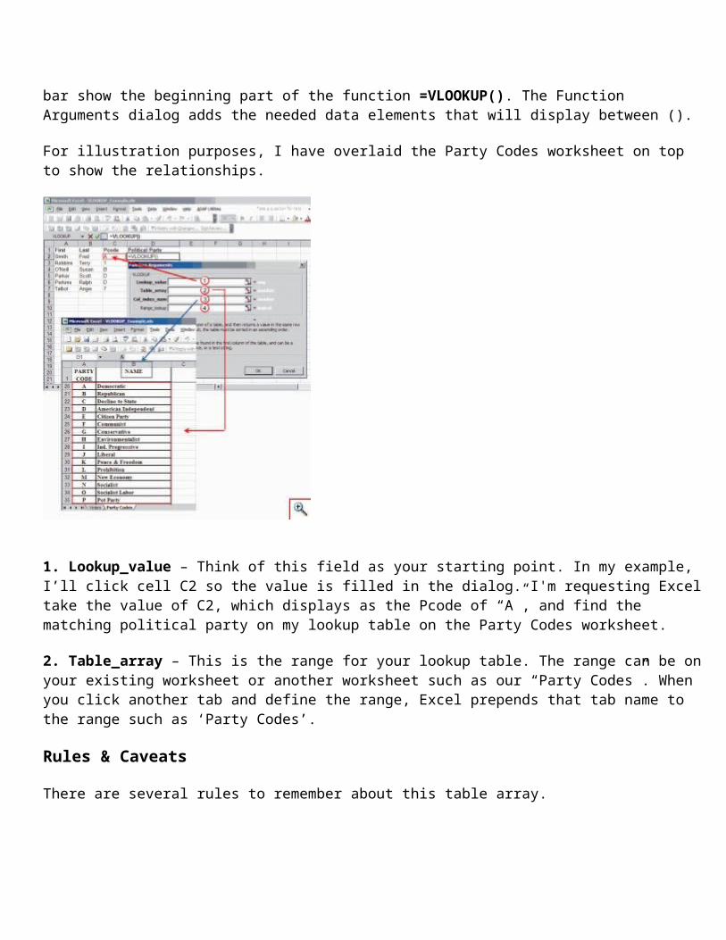
After you click OK, Excel’s Function Arguments dialog appears and allows you to define the four values. You’ll see that your starting cell and the formula bar show the beginning part of the function =VLOOKUP(). The Function Arguments dialog adds the needed data elements that will display between ().

For illustration purposes, I have overlaid the Party Codes worksheet on top to show the relationships.

1. Lookup_value – Think of this field as your starting point. In my example, I’ll click cell C2 so the value is filled in the dialog. I'm requesting Excel take the value of C2, which displays as the Pcode of “A”, and find the matching political party on my lookup table on the Party Codes worksheet.

2. Table_array – This is the range for your lookup table. The range can be on your existing worksheet or another worksheet such as our “Party Codes”. When you click another tab and define the range, Excel prepends that tab name to the range such as ‘Party Codes’.

Rules & Caveats

There are several rules to remember about this table array.

Rule 1 - The left column must contain the values being referenced. In other words, I couldn’t have our first column be Political Party.

Rule 2 - You can’t have duplicate values in the leftmost column of the lookup range. I couldn’t have two entries with the value “A” with one being “Democratic” party and another “A” for the “Humanist” party. Excel would complain.

Rule 3 - When referencing a lookup table, you don’t want your cell references to change when you drag and fill to populate the other cells with the VLOOKUP function. As example, if I want to use the same function in cells D3 through D7, I don’t want my lookup cell references to shift each time I move down to the next cell. I need the cell references to be the same. After you define your range, you need to press F4 which will cycle through

absolute and relative references. You want to select the option that includes a $ before your Column and Row. ( 'Party Codes'!$A$2:$B$45. ) You can get around this if you know how to use Excel name ranges.

Col_index_num – This is the number of the column on your lookup table that has the information you need. In our example, we want column 2 from the Party Codes worksheet which has the name of the political party.

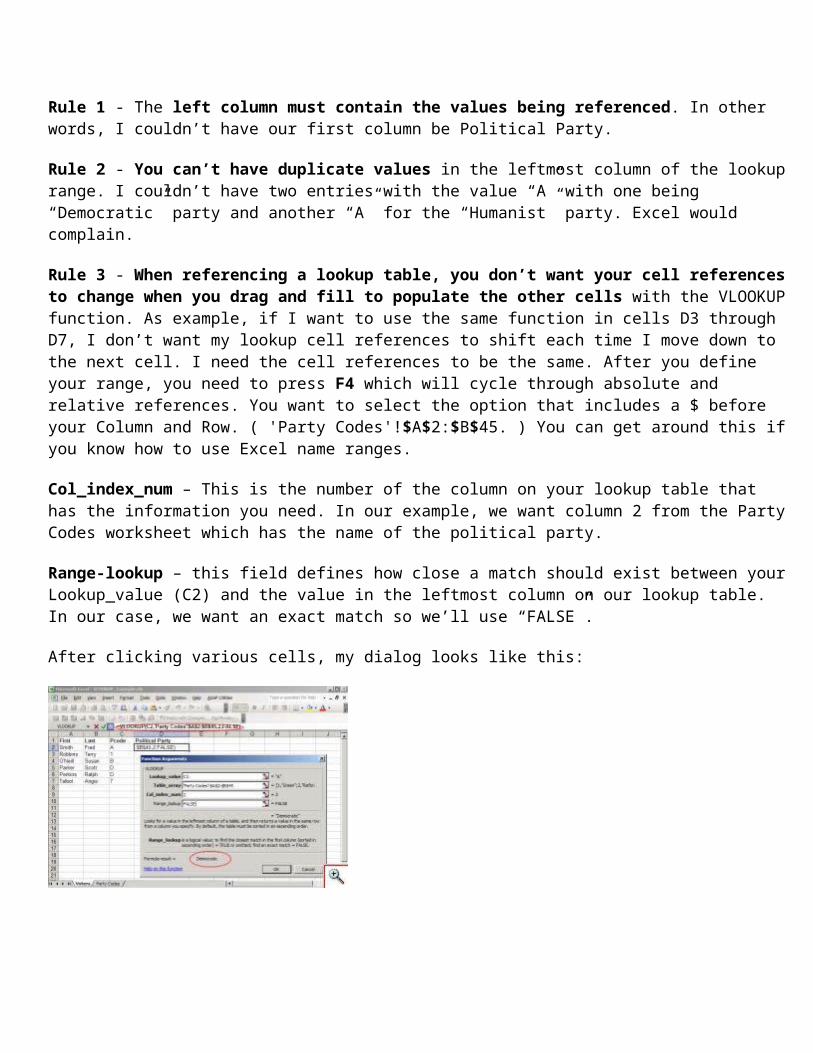
Range-lookup – this field defines how close a match should exist between your Lookup_value (C2) and the value in the leftmost column on our lookup table. In our case, we want an exact match so we’ll use “FALSE”.

After clicking various cells, my dialog looks like this:

You can see in the circled formula bar above, I now have more information based on my entries in the Function Arguments dialog box.

The other item of interest is that when you build these functions, Excel displays the result in the Formula result = text line. This is great feedback which can show if your function is on target. In our example, we can see Excel looked up the Pcode of “A” and returned the Political Party “Democratic”.

Copying the VLOOKUP Function to Other Cells

It doesn’t make sense to use VLOOKUP for one cell in your Excel spreadsheet. Instead, I want to copy the function to other cells in the same column.

To copy VLOOKUP to other column cells,

1. Click the cell containing the VLOOKUP arguments. In our example, this would be D2.

2. Grab the cell handle that displays in the lower right corner.

3. Left-click and drag down the cell handle to cover your column range.

Note: If I hadn’t changed to absolute reference as mentioned in Rule 3, I would’ve seen my table array entry shift by one cell as we dragged down through the other cells.

VLOOKUP is a powerful Excel function that can leverage spreadsheet data from other sources. There are many ways you can benefit from this function. In this example, I used a 1:1 code translation, but you could also use it for group assignments. For example, you could assign state codes to a region such as CT, VT, and MA to a region called “New England”. And for the adventurous, you can use VLOOKUP in your Excel formulas.

MS Excel: HLookup Function

In Excel, the HLookup function searches for value in the top row of table_array and returns the value in the same column based on the index_number.

The syntax for the HLookup function is:

HLookup( value, table_array, index_number, not_exact_match )

value is the value to search for in the first row of the table_array.

table_array is two or more rows of data that is sorted in ascending order.

index_number is the row number in table_array from which the matching value must be returned. The first row is 1.

not_exact_match determines if you are looking for an exact match based on value. Enter FALSE to find an exact match. Enter TRUE to find an approximate match, which means that if an exact match if not found, then the HLookup function will look for the next largest value that is less than value.

Note:

If index_number is less than 1, the HLookup function will return #VALUE!.

If index_number is greater than the number of columns in table_array, the HLookup function will return #REF!.

If you enter FALSE for the not_exact_match parameter and no exact match is found, then the HLookup function will return #N/A.

Applies To:

Excel 2007, Excel 2003, Excel XP, Excel 2000

For example:

Let's take a look at an example:

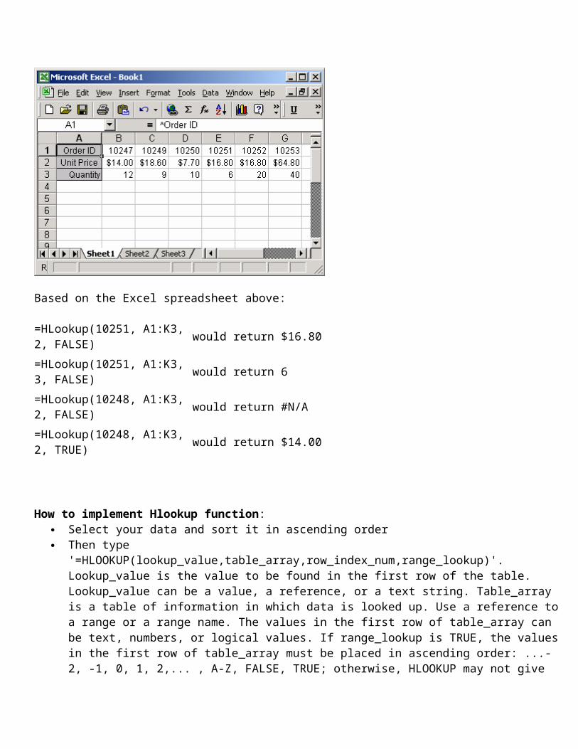
Based on the Excel spreadsheet above:

=HLookup(10251, A1:K3, 2, FALSE)

would return $16.80

=HLookup(10251, A1:K3, 3, FALSE)

would return 6

=HLookup(10248, A1:K3, 2, FALSE)

would return #N/A

=HLookup(10248, A1:K3, 2, TRUE)

would return $14.00

How to implement Hlookup function: Select your data and sort it in ascending order Then type '=HLOOKUP(lookup_value,table_array,row_index_num,range_lookup)'.

Lookup_value is the value to be found in the first row of the table. Lookup_value can be a value, a reference, or a text string. Table_array is a table of information in which data is looked up. Use a reference to a range or a range name. The values in the first row of table_array can be text, numbers, or logical values. If range_lookup is TRUE, the values in the first row of table_array must be placed in ascending order: ...-2, -1, 0, 1, 2,... , A-Z, FALSE, TRUE; otherwise, HLOOKUP may not give the correct value.If range_lookup is FALSE, table_array does not need to be sorted. Uppercase and lowercase text are

equivalent. You can put values in ascending order, left to right, by selecting the values and then clicking Sort on the Data menu. Click Options in the sort dialog box, click Sort left to right, and then click OK. Under Sort by, click the row in the list, and then click Ascending.Row_index_num is the row number in table_array from which the matching value will be returned. A row_index_num of 1 returns the first row value in table_array, a row_index_num of 2 returns the second row value in table_array, and so on. If row_index_num is less than 1, HLOOKUP returns the #VALUE! error value; if row_index_num is greater than the number of rows on table_array, HLOOKUP returns the #REF! error value.Range_lookup is a logical value that specifies whether you want HLOOKUP to find an exact match or an approximate match. If TRUE or omitted, an approximate match is returned. In other words, if an exact match is not found, the next largest value that is less than lookup_value is returned. If FALSE, HLOOKUP will find an exact match. If one is not found, the error value #N/A is returned.

If HLOOKUP can't find lookup_value, and range_lookup is TRUE, it uses the largest value that is less than lookup_value.

If lookup_value is smaller than the smallest value in the first row of table_array, HLOOKUP returns the #N/A error value.

If range_lookup is FALSE and lookup_value is text, you can use the wildcard characters, question mark (?) and asterisk (*), in lookup_value. A question mark matches any single character; an asterisk matches any sequence of characters. If you want to find an actual question mark or asterisk, type a tilde (~) before the character.

In the example in the Excel training video the sorted data represents the density of water at different temperatures. The left most column gives the temperature in degrees and the top column specifies the 'decimal' degrees

We looked up the density of water at 5.4 degrees celsius using the Hlookupfunction.

What is a Pivot Table?

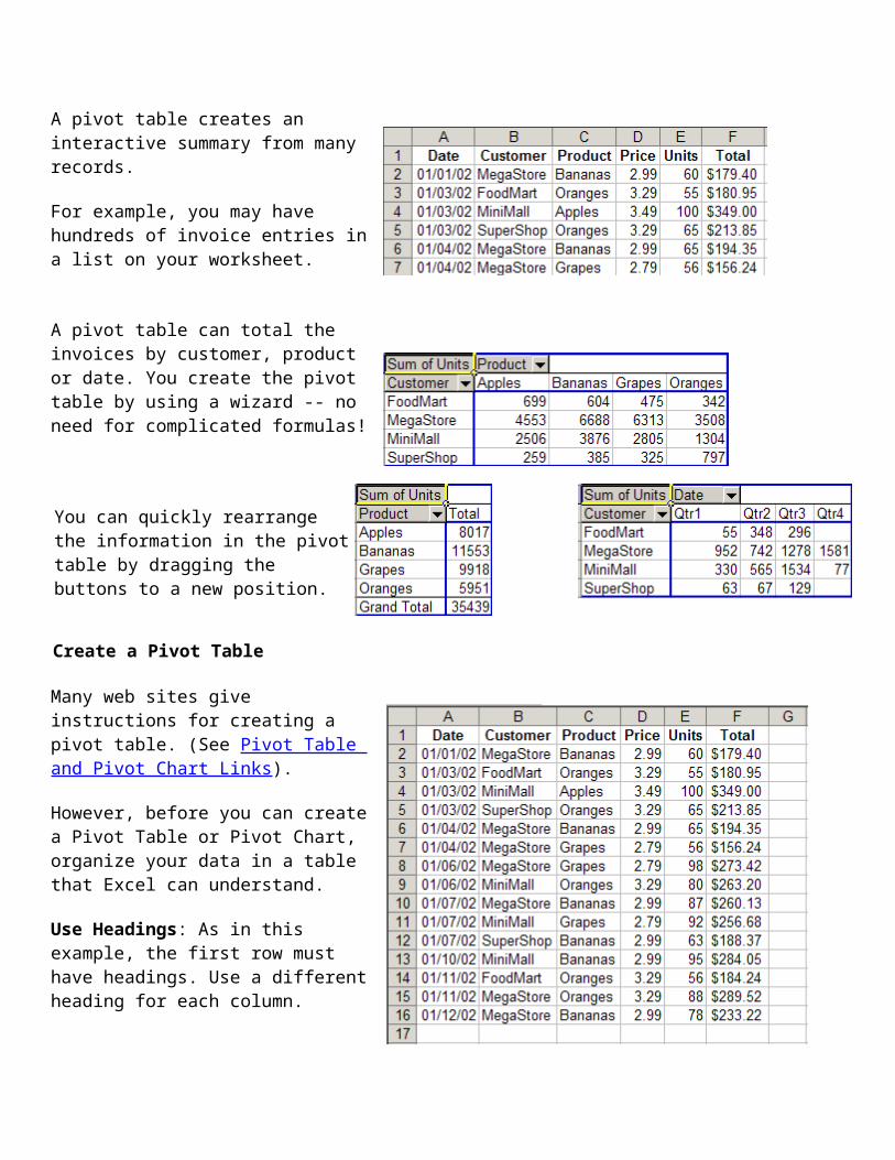
A pivot table creates an interactive summary from many records.

For example, you may have hundreds of invoice entries in a list on your worksheet.

 

A pivot table can total the invoices by customer, product or date. You create the pivot table by using a wizard -- no need for complicated formulas!

 

You can quickly rearrange the information in the pivot table by dragging the buttons to a new position.

Create a Pivot Table

Many web sites give instructions for creating a pivot table. (See Pivot Table and Pivot Chart Links).

However, before you can create a Pivot Table or Pivot Chart, organize your data in a table that Excel can understand.

Use Headings: As in this example, the first row must have headings. Use a different heading for each column.

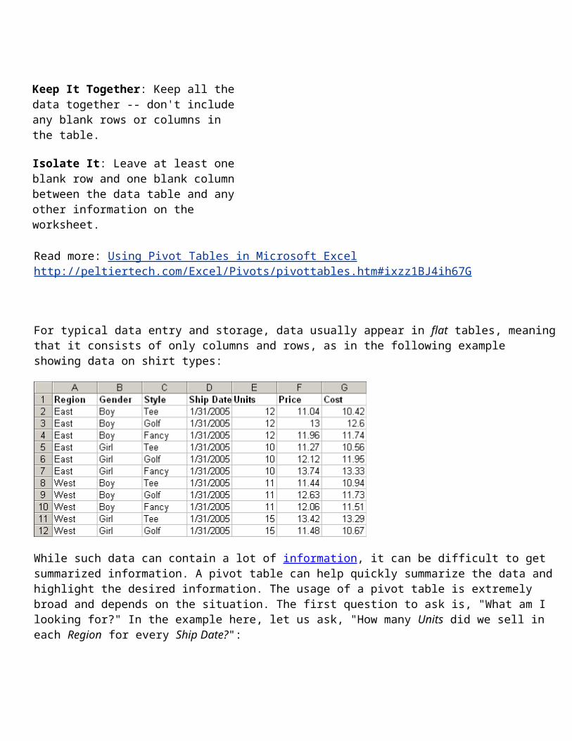
Keep It Together: Keep all the data together -- don't include any blank rows or columns in the table.

Isolate It: Leave at least one blank row and one blank column between the data table and any other information on the worksheet.

Read more: Using Pivot Tables in Microsoft Excel http://peltiertech.com/Excel/Pivots/pivottables.htm#ixzz1BJ4ih67G

For typical data entry and storage, data usually appear in flat tables, meaning that it consists of only columns and rows, as in the following example showing data on shirt types:

While such data can contain a lot of information, it can be difficult to get summarized information. A pivot table can help quickly summarize the data and highlight the desired information. The usage of a pivot table is extremely broad and depends on the situation. The first question to ask is, "What am I looking for?" In the example here, let us ask, "How many Units did we sell in each Region for every Ship Date?":

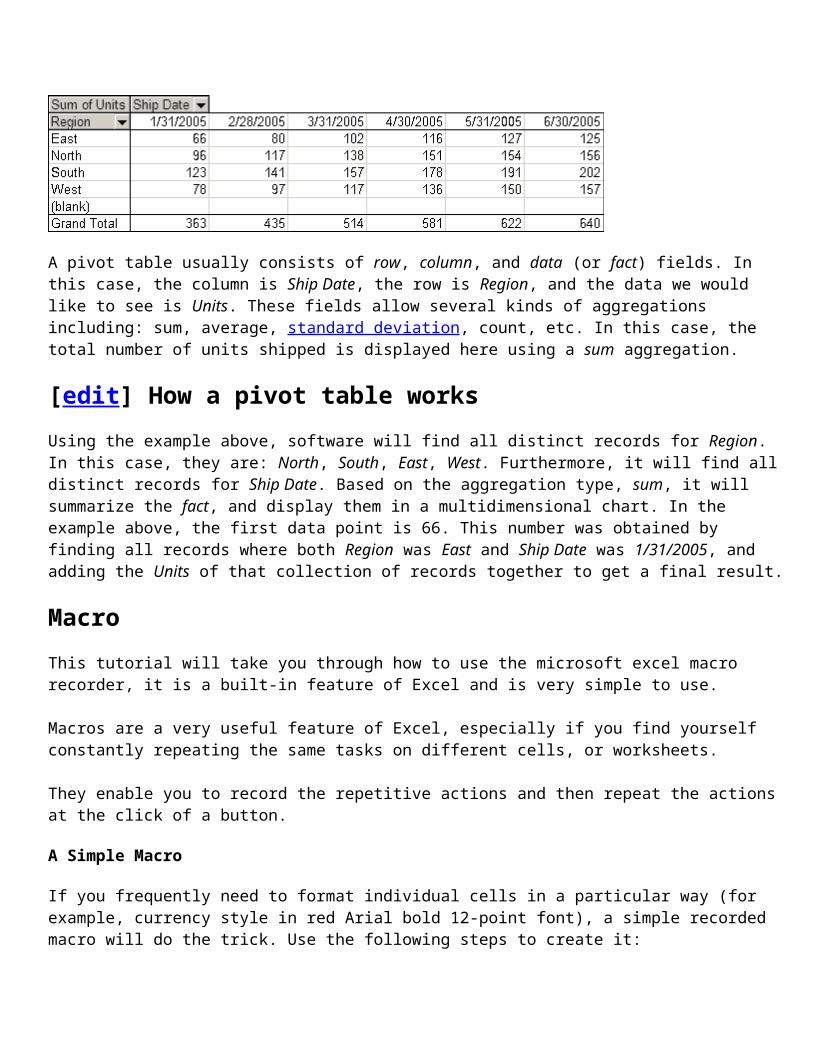
A pivot table usually consists of row, column, and data (or fact) fields. In this case, the column is Ship Date, the row is Region, and the data we would like to see is Units. These fields allow several kinds of aggregations including: sum, average, standard deviation, count, etc. In this case, the total number of units shipped is displayed here using a sum aggregation.

[edit] How a pivot table works

Using the example above, software will find all distinct records for Region. In this case, they are: North, South, East, West. Furthermore, it will find all distinct records for Ship Date. Based on the aggregation type, sum, it will summarize the fact, and display them in a multidimensional chart. In the example above, the first data point is 66. This number was obtained by finding all records where both Region was East and Ship Date was 1/31/2005, and adding the Units of that collection of records together to get a final result.

Macro

This tutorial will take you through how to use the microsoft excel macro recorder, it is a built-in feature of Excel and is very simple to use.

Macros are a very useful feature of Excel, especially if you find yourself constantly repeating the same tasks on

different cells, or worksheets.

They enable you to record the repetitive actions and then repeat the actions at the click of a button.

A Simple Macro

If you frequently need to format individual cells in a particular way (for example, currency style in red Arial bold 12-point font), a simple recorded macro will do the trick. Use the following steps to create it:

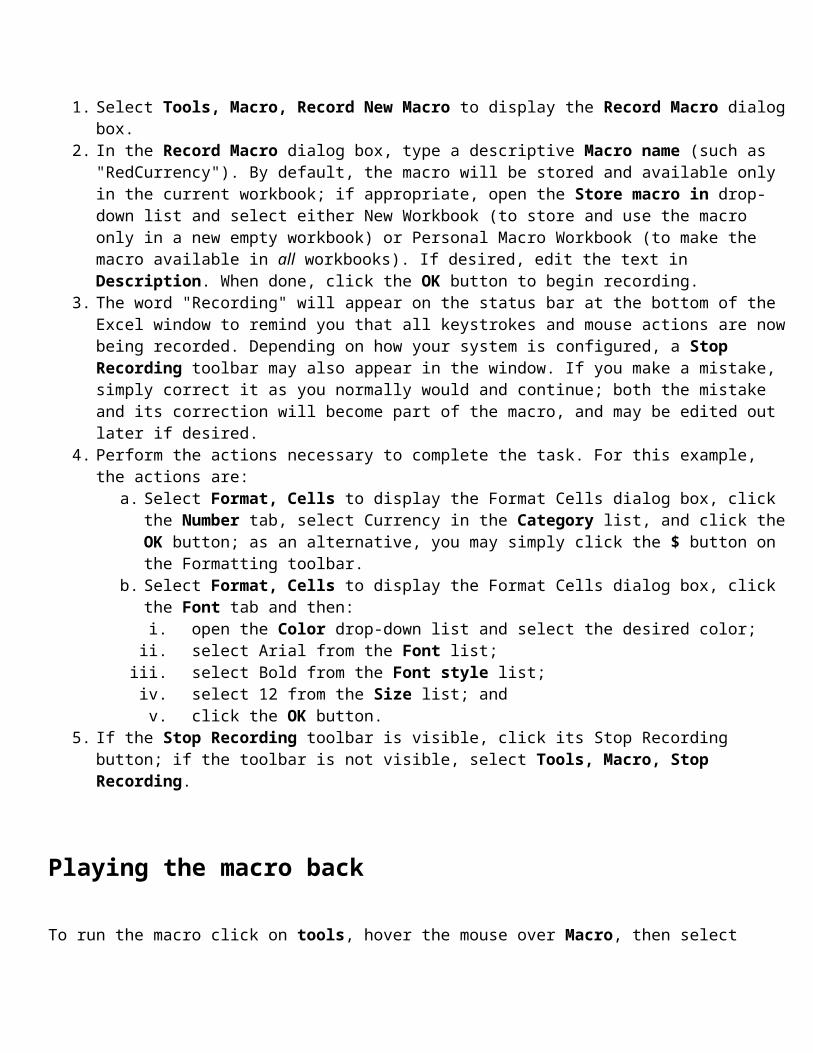
1. Select Tools, Macro, Record New Macro to display the Record Macro dialog box.2. In the Record Macro dialog box, type a descriptive Macro name (such as "RedCurrency"). By default, the

macro will be stored and available only in the current workbook; if appropriate, open the Store macro in drop-down list and select either New Workbook (to store and use the macro only in a new empty workbook) or Personal Macro Workbook (to make the macro available in all workbooks). If desired, edit the text in Description. When done, click the OK button to begin recording.

3. The word "Recording" will appear on the status bar at the bottom of the Excel window to remind you that all keystrokes and mouse actions are now being recorded. Depending on how your system is configured, a Stop Recording toolbar may also appear in the window. If you make a mistake, simply correct it as you normally would and continue; both the mistake and its correction will become part of the macro, and may be edited out later if desired.

4. Perform the actions necessary to complete the task. For this example, the actions are:a. Select Format, Cells to display the Format Cells dialog box, click the Number tab, select Currency

in the Category list, and click the OK button; as an alternative, you may simply click the $ button on the Formatting toolbar.

b. Select Format, Cells to display the Format Cells dialog box, click the Font tab and then:i. open the Color drop-down list and select the desired color;

ii. select Arial from the Font list;iii. select Bold from the Font style list;iv. select 12 from the Size list; andv. click the OK button.

5. If the Stop Recording toolbar is visible, click its Stop Recording button; if the toolbar is not visible, select Tools, Macro, Stop Recording.

Playing the macro back

To run the macro click on tools, hover the mouse over Macro, then select Macros.

You will see the Macro dialogue box similar to that shown in fig 1.3 below, your macro should be in there ready to use.

To use the macro simply select it and then click the Run button.

The macro dialogue box also allows you to delete and edit macros, for instance by clicking on the Options button you can assign or change the keyboard shortcut associated with each macro.

If you have assigned a keyboard shortcut to a macro then you can run it by holding down the CTRL key and pressing the associated letter.

Mail Merge in Excel faq68-4223Posted: 24 Sep 03 (Edited 21 Dec 10)

Mail Merge in Word has some limitations.

Here's a way to perform a Mail Merge in Excel.

A. Setting up the data.

 1. Make a separate sheet for your data table 2. If your data is in another application like Access, use Data/Get External data to query the columns and rows that you want.    If your data is already in Excel, if you have formatted your table properly (one table per sheet, headings in row 1 starting in column A, table is contiguous) then you can use the technique in step 2 as well.

B. Setting up the "form"

   The objective is to MAP data from selected columns in your Source Data Table to the Form, using Named Ranges.  If you do not know what a Named Range is, please refer to Excel HELP.

 1. Format the page(s) the way that you want your form to look 2. Each Merge Cell should have no other data in it. 3. Each Merge Cell should be named with the same name as the column heading on the data sheet.      NOTE: if any data column heading contains a space, then substitute an UNDERSCORE character for each space. For instance, a data heading like First Name should have a corresponding Merge Field name of First_Name.

C. Running Mail Merge

 1. Select the rows that you want from your data using the AutoFilter or Advanced Filter if you filter in place. 2. Run MergePrint from Tools/Macro/Macros or a button.  

D. The code that runs the Mail Merge

This page lists the current, built-in Excel Logical Functions. These functions are provided by Excel, to help you to work the logical values, TRUE and FALSE. They include boolean operators, conditional tests and functions to return the constant logical values.

The functions have been grouped into categories, to help you to find the function you need to perform a specific task. Selecting a function name will take you to a full description of the function, with examples of use.

Excel Logical Functions List

Boolean Operator Functions

AND Tests a number of user-defined conditions and returns TRUE if ALL of the conditions evaluate to TRUE, or FALSE otherwise

OR Tests a number of user-defined conditions and returns TRUE if ANY of the conditions evaluate to TRUE, or FALSE otherwise

NOT Returns a logical value that is the opposite of a user supplied logical value or expression(ie. returns FALSE is the supplied argument is TRUE and returns TRUE if

Conditional Functions

IF Tests a user-defined condition and returns one result if the condition is TRUE, and another result if the condition is FALSE

IFERROR Tests if an initial supplied value (or expression) returns an error, and if so the function returns a supplied value; Otherwise the function returns the initial value. (New in Excel 2007)

Functions Returning Constant Values

the supplied argument is FALSE) TRUE Simply returns the logical value TRUE

FALSE Simply returns the logical value FALSE

A logical function is one that can return a true value or a false value. They are usually used in doing comparisons and seeing if things are equal to each other or not, or which is higher or lower. The logical functions that Excel provides are:

TRUE FALSE AND OR NOT

Read more: http://wiki.answers.com/Q/Define_logical_function_in_excel#ixzz1BJ8TBJ5z

MS Excel: Transpose FunctionExcel: Transpose Data

If you have data in columns and you wish that data were in rows (or if you have data in rows that you wish were in columns), you do not need to retype it.

1. Simply select the data and hit the Copy button. 2. Next, select the cell that you want to become the upper left corner of the new range of data. 3. Go to the menu bar and choose Edit | Paste Special. In the Paste Special dialog box, choose Transpose.

In Excel, the Transpose function returns a transposed range of cells. For example, a horizontal range of cells is returned if a vertical range is entered as a parameter. Or a vertical range of cells is returned if a horizontal range of cells is entered as a parameter.

The syntax for the Transpose function is:

Transpose( range )

range is the range of cells that you want to transpose.

Note:

The range value in the Transpose function must be entered as an array. To enter an array, enter the value and then press Ctrl-Shift-Enter. This will place {} brackets around the formula, indicating that it is an array.

Applies To:

Excel 2007, Excel 2003, Excel XP, Excel 2000

For example:

Let's take a look at an example:

Based on the Excel spreadsheet above:

We've placed values in cells A1, A2, and A3, and we'd like to view these values in cells C1, D1, and E1 (transposed). To do this, you highlight cells C1, D1, and E1, then enter the following formula:

=TRANSPOSE(A1:A3)

Then press Ctrl-Shift-Enter to create an array formula. You will notice that {} brackets will appear around the formula and the values in cells A1, A2, and A3 should now appear in cells C1, D1, and E1.

Frequently Asked Questions

Question:  In Excel, isn't it easier to use the Paste Special transpose option to do the same?

Answer: Yes, if you ONLY want to perform a one-time paste of the values, you can do the following:

Highlight the cells that you want to copy. In this example, we've highlighted cells A1:A3. Then right-click and select Copy from the popup menu.

Then right-click on the cell where you'd like to paste the values and select Paste Special from the popup menu.

Then select the Transpose checkbox and click on the OK button.

Now when you return to your spreadsheet, you'll see that the values have been copied and transposed.