Gestion de la production - lamsade.dauphine.frfurini/lib/exe/fetch.php?media=wiki:notes... ·...

Gestion de la production

• Book: Linear Programming, Vasek Chvatal, McGill University, W.H. Freeman and Com-pany, New York, USA

1

Contents

1 Integer Linear Programming 31.1 Definitions and notations . . . . . . . . . . . . . . . . . . . . . . . . . . . . . . . . . . . . . . 31.2 Solvers . . . . . . . . . . . . . . . . . . . . . . . . . . . . . . . . . . . . . . . . . . . . . . . . . 51.3 Example . . . . . . . . . . . . . . . . . . . . . . . . . . . . . . . . . . . . . . . . . . . . . . . . 61.4 LibreOffice Solver . . . . . . . . . . . . . . . . . . . . . . . . . . . . . . . . . . . . . . . . . 81.5 Branch-And-Bound Algorithm . . . . . . . . . . . . . . . . . . . . . . . . . . . . . . . . . . . 111.6 Minimization of concave piece-wise affine functions . . . . . . . . . . . . . . . . . . . . . . . . 191.7 Minimization of convex piece-wise affine functions . . . . . . . . . . . . . . . . . . . . . . . . 231.8 Constraints with absolute value expressions . . . . . . . . . . . . . . . . . . . . . . . . . . . . 251.9 Minimization of objective functions with absolute values . . . . . . . . . . . . . . . . . . . . . 261.10 Soft Constraints, Big-M constraints, Alldiff constraints . . . . . . . . . . . . . . . . . . . . . 271.11 Boolean expressions using binary variables . . . . . . . . . . . . . . . . . . . . . . . . . . . . . 291.12 Lagrangian Relaxations . . . . . . . . . . . . . . . . . . . . . . . . . . . . . . . . . . . . . . . 31

2 Capacitated Lot-Sizing problems 342.1 Capacitated Lot-Sizing problems with setups . . . . . . . . . . . . . . . . . . . . . . . . . . . 38

2.1.1 Formulation 1 . . . . . . . . . . . . . . . . . . . . . . . . . . . . . . . . . . . . . . . . . 392.1.2 Formulation 2 . . . . . . . . . . . . . . . . . . . . . . . . . . . . . . . . . . . . . . . . . 39

3 Scheduling of jobs 413.1 Solution techniques . . . . . . . . . . . . . . . . . . . . . . . . . . . . . . . . . . . . . . . . . . 433.2 Dispatching rules . . . . . . . . . . . . . . . . . . . . . . . . . . . . . . . . . . . . . . . . . . . 433.3 Classification of Scheduling problems . . . . . . . . . . . . . . . . . . . . . . . . . . . . . . . . 443.4 Problems on a single machine . . . . . . . . . . . . . . . . . . . . . . . . . . . . . . . . . . . . 453.5 Problems on parallel machines . . . . . . . . . . . . . . . . . . . . . . . . . . . . . . . . . . . 453.6 Shop Problems . . . . . . . . . . . . . . . . . . . . . . . . . . . . . . . . . . . . . . . . . . . . 46

4 Job assignment to machines with ILP models 484.1 Production plans with precedence constraints . . . . . . . . . . . . . . . . . . . . . . . . . . . 484.2 Load balancing between different machines . . . . . . . . . . . . . . . . . . . . . . . . . . . . 494.3 Sequencing of jobs on a single machine . . . . . . . . . . . . . . . . . . . . . . . . . . . . . . . 51

5 Heuristic Algorithms 545.1 Genetic Algorithms . . . . . . . . . . . . . . . . . . . . . . . . . . . . . . . . . . . . . . . . . . 57

2

1 Integer Linear Programming

1.1 Definitions and notations

An integer linear program is a linear program with the additional constraint that the variables are requiredto be integer.

Z(ILP)= min c>x (1)

Ax ≥ b (2)

x ∈ Z+ (3)

where A ∈ Rm·n , b ∈ Rm, c ∈ Rn.

INPUT DATA : A =

a11 a12 . . . a1na21 a22 . . . a2n. . . . . . . . . . . .am1 am2 . . . amn

b =

b1b2. . .bm

c =

c1c2. . .. . .. . .cn

VARIABLES : x =

x1x2. . .. . .. . .xn

Equivalent way an writing an ILP:

Z(ILP)= min

n∑j=1

cjxj (4)

n∑j=1

aijxj ≥ bi i = 1, . . . ,m (5)

xj ∈ Z+ j = 1, . . . , n (6)

• Z(LP) is a valid bound for Z(ILP):

– lower bound in case of minimization

– upper bound in case of maximization

• Definition: ∀y ∈ R, the integer part of y is byc =max integer q : q ≤ y

• if cj ∈ Z (∀j = 1, . . . , n):

– for minimization bZ(LP )c+ 1 is a valid lower bound for Z(ILP)

– for maximization bZ(LP )c is a valid upper bound for Z(ILP)

Example:

A =

[50 31−3 2

]b =

[2504

]c =

[1

0.64

]x =

[x1x2

] Z(ILP) = max x1 + 0.64x250x1 + 31x2 ≤ 250−3x1 + 2x2 ≤ 4x1, x2 ∈ Z+

• the optimal LP solution value is Z(LP)= 984193 ≈ 5.09

• Z(LP) is an upper bound for Z(ILP) −→ upper bound = 984193 ≈ 5.09

3

x1

x2

(0, 2)

x∗2 = 950193 ≈ 4.92

x∗1 = 376193 ≈ 1.94

Z(LP)= 984193 ≈ 5.09

∇f(x) =[1 0.64

](5, 0)

(0, 25031 ≈ 8.064)

Z(ILP)=5

• the optimal LP solution x∗LP =

[376193

950193

]−→ very far from the optimal integer solution

• the optimal solution value is Z(ILP)=5

• the optimal solution x∗ =

[5

0

]

Definition – Mixed Integer Linear Program (MILP)An ILP when some variables are restricted to be integer and some are not, the problem is called: mixedinteger linear program.

Z(MILP)= min c>x (7)

Ax ≥ b (8)

x ≥ 0 (9)

xj ∈ Z+ j = 1, . . . , p (10)

Definition – Binary program (BP)An ILP where the integer variables are restricted to be 0 or 1 (it comes up surprisingly often). Such problemsare called pure (mixed) 0–1 linear programs or pure (mixed) binary integer linear programs.

Z(BP)= min c>x (11)

Ax ≥ b (12)

x ∈ {0, 1} (13)

4

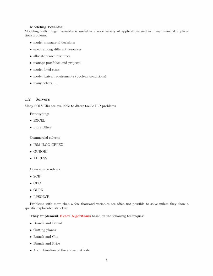
Modeling PotentialModeling with integer variables is useful in a wide variety of applications and in many financial applica-tion/problems:

• model managerial decisions

• select among different resources

• allocate scarce resources

• manage portfolios and projects

• model fixed costs

• model logical requirements (boolean conditions)

• many others . . .

1.2 Solvers

Many SOLVERs are available to direct tackle ILP problems.

Prototyping:

• EXCEL

• Libre Office

Commercial solvers:

• IBM ILOG CPLEX

• GUROBI

• XPRESS

Open source solvers:

• SCIP

• CBC

• GLPK

• LPSOLVE

Problems with more than a few thousand variables are often not possible to solve unless they show aspecific exploitable structure.

They implement Exact Algorithms based on the following techniques:

• Branch and Bound

• Cutting planes

• Branch and Cut

• Branch and Price

• A combination of the above methods

5

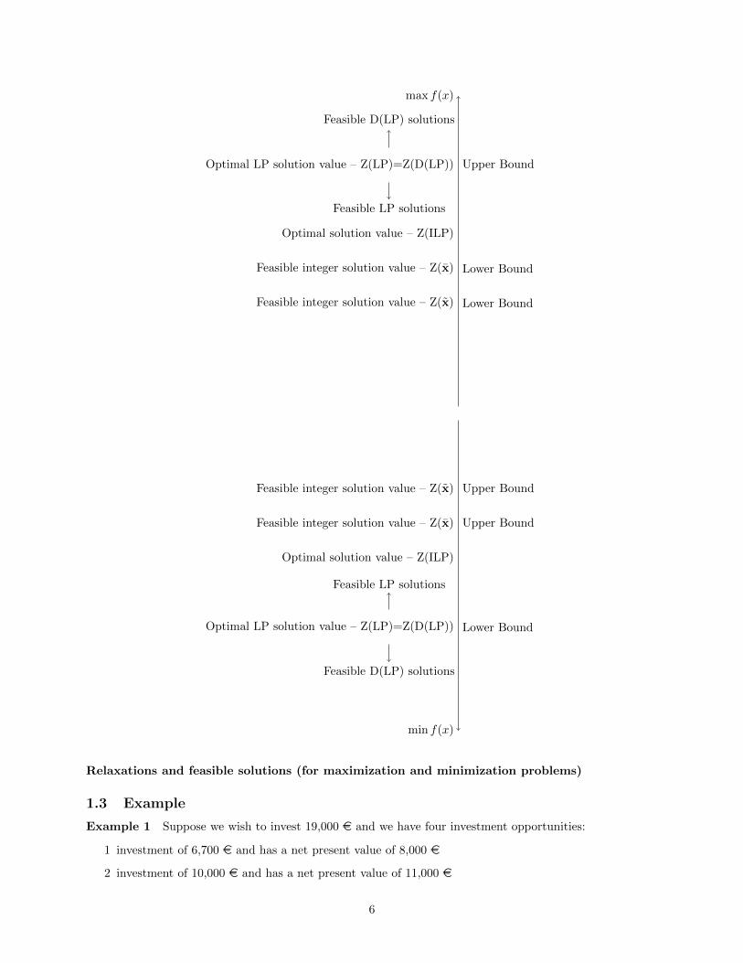
max f(x)

Feasible D(LP) solutions

Feasible LP solutions

Optimal solution value – Z(ILP)

Optimal LP solution value – Z(LP)=Z(D(LP)) Upper Bound

Feasible integer solution value – Z(x) Lower Bound

Feasible integer solution value – Z(x) Lower Bound

min f(x)

Feasible LP solutions

Feasible D(LP) solutions

Optimal solution value – Z(ILP)

Optimal LP solution value – Z(LP)=Z(D(LP)) Lower Bound

Feasible integer solution value – Z(x) Upper Bound

Feasible integer solution value – Z(x) Upper Bound

Relaxations and feasible solutions (for maximization and minimization problems)

1.3 Example

Example 1 Suppose we wish to invest 19,000 e and we have four investment opportunities:

1 investment of 6,700 e and has a net present value of 8,000 e


6



Into which investments should we place our money so as to maximize our total present value? Suchproblems are called capital budgeting problems.

Decision variables:

xj =

{1 if investment j is made (j = 1, . . . , 4)0 otherwise

max 8, 000x1 + 11, 000x2 + 6, 000x3 + 4, 000x4 (14)

6, 700x1 + 10, 000x2 + 5.500x3 + 3, 400x4 ≤ 19, 000 (15)

xi ∈ {0, 1} i = 1, 2, 3, 4 (16)

Ignoring integrality constraints: the optimal linear programming solution is:

• the optimal linear programming solution is: x1=1, x2=0.89, x3= 0, x4 = 1

• the optimal LP solution value is 21,790 e

• this solution is not integral

• rounding x2 down to 0 gives a feasible integer solution of value of 12,000 e

• the optimal solution is: x1=0, x2=1, x3= 1, x4 = 1

• the optimal solution value is 21,000 e

There are a number of additional constraints we can add:

• Only a maximum of two investments can be made

x1 + x2 + x3 + x4 ≤ 2

• If investment 2 is made, then investment 4 must also be made (if investment 4 is not made then either2 is made)

x2 − x4 ≤ 0

x2 x40 0 OK1 1 OK0 1 OK1 0 NOT OK

• If investment 1 is made, then investment 3 cannot be made (if investment 3 is made then 1 cannot bemade)

x1 + x3 ≤ 1

x1 x30 0 OK0 1 OK1 0 OK1 1 NOT OK

• the optimal solution is: x1=0, x2=1, x3= 0, x4 = 1

• the optimal solution value is 15,000 e

7

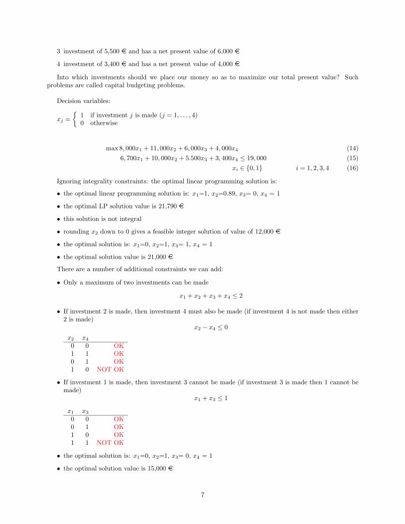
1.4 LibreOffice Solver

• Step-by-step description of the solution of Example 1 using the solver provided by LibreOffice

• the spreadsheet of the model is presented by the following figure

• the blue cells represent the input data of the model

The model is composed by three parts

• the variables represented by cells E13,F13,G13,H13

• the objective function represented by cell D5

• the constraints represented by rows 17,19,21, 23.

• the first two constraints are represented in the figures

• the solution of the model is computed using the solver

8

• the variables are constraint to have binary values as shown in the figure

• before solving the model is it necessary to set the options

• pressing the bottom solve you get the optimal solution and the optimal solution value

9

1.5 Branch-And-Bound Algorithm

• Branch and bound has been the most effective technique for solving MILPs in the following forty yearsor so (it was proposed in 1960 by Land and Dong).

• It is based on dividing the problem into a number of smaller problems (branching) and evaluating theirquality based on solving the underlying linear programs (bounding).

• However, in the last ten years, cutting planes have made a resurgence and are now efficiently combinedwith branch and bound into an overall procedure called branch and cut (this term was coined by in1987 by Padberg and Rinaldi).

The goal is to solve an integer linear program (ILP):

Z(ILP)= min

n∑j=1

cjxj (17)

n∑j=1

aijxj ≥ bi i = 1, . . . ,m (18)

xj ∈ Z+ j = 1, . . . , n (19)

• where matrix A ∈ Rm·n , m-vector b ∈ Rm, n-vector c ∈ Rn.

• The technique can be extended to MILP.

Bounding : the engine of the branch and bound algorithm is the solution of the Linear ProgrammingRelaxation of the ILP:

Z(LP)= min

n∑j=1

cjxj (20)

n∑j=1

aijxj ≥ bi i = 1, . . . ,m (21)

xj ≥ 0 j = 1, . . . , n (22)

11

• The best known (and most successful) methods for solving LPs is the simplex algorithm.

• Rounding the solution of the LP will not in general give the optimal solution of the ILP.

• Since the the LP is less constrained than an ILP, the following are immediate:

– The optimal objective value for the LP is less than or equal to the optimal objective for the ILP

– If the LP is infeasible, then so is ILP

– If the optimal solution x∗ of the LP satisfies x∗i integer for i = 1, ..., n, then x∗ is also optimal forthe ILP

– Otherwise, it gives a bound on the optimal value of the ILP

Notation and data structure

• The branch-and-bound algorithm keeps a list of linear programming problems obtained by relaxing theintegrality requirements on the variables and imposing constraints such as:

– xj ≤ uj– xj ≥ lj

• Each such linear program corresponds to a node of the branch-and-bound tree.

• For a node Ni , let Z(Ni) denote the optimal solution value of the corresponding linear program.

• Let L denote the list of nodes that must still be solved.

• Let ZB denote a valid bound on the optimum value (initially, the bound ZB can be derived from aheuristic ILP solution, or it can be set to +∞ (-∞) in case of maximization).

Pseudo code of the algorithm (minimization)

Step 0 Initialize L = LP, ZB = +∞, x∗ = ∅.

Step 1 Terminate? If L = ∅, the solution x∗ is optimal.

Step 2 Select node Choose and delete a problem Ni from L.

Step 3 Bound Solve Ni . If it is infeasible, go to Step 1. Else, let xi be its solution and Z(Ni) its objectivevalue.

Step 4 Prune

– If Z(Ni) ≥ ZB , go to Step 1.

– If xi is not feasible for ILP, go to Step 5.

– If xi is feasible for ILP, let ZB = Z(Ni) , x∗ = xi. Delete from L all problems with Z(Nj) ≥ ZB .Go to Step 1.

Step 5 Branch From Ni , construct linear programs N1i , . . . , N

ki with smaller feasible regions whose union

contains all the feasible solutions of (MILP) in Ni . Add N1i , . . . , N

ki to L and go to Step 1.

12

Pseudo code of the algorithm (maximization)

• All the steps remains unchanged except:

Step 0 Initialize L = ILP, ZB = -∞, x∗ = ∅.

Step 4 Prune

– If Z(Ni)≤ZB , go to Step 1.

– If xi is not feasible for MILP, go to Step 5.

– If xi is feasible for ILP, let ZB = Z(Ni) , x∗ = xi. Delete from L all problems with Z(Nj)≤ZB .Go to Step 1.

We can stop the enumeration at a node of the branch-and-bound tree for three different reasons (whenthey occur, the node is said to be pruned).

• Pruning by integrality occurs when the corresponding linear program has an optimum solution thatis integral.

• Pruning by bounds occurs when the objective value of the linear program at that node is worse thanthe value of the best feasible solution found so far.

• Pruning by infeasibility occurs when the linear program at that node is infeasible.

• Optimal LP solutions are at the intersections of linear constraints (or on one of them)

• Point of intersection (α, β) = ( c·s−b·tb·r−a·s ,

a·t−c·rb·r−a·s ) among two lines:{

a · x1 + b · x2 + c = 0r · x1 + s · x2 + t = 0

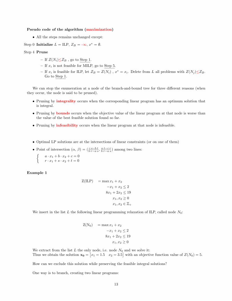
Example 1

Z(ILP) = maxx1 + x2

−x1 + x2 ≤ 2

8x1 + 2x2 ≤ 19

x1, x2 ≥ 0

x1, x2 ∈ Z+

We insert in the list L the following linear programming relaxation of ILP, called node N0:

Z(N0) = maxx1 + x2

−x1 + x2 ≤ 2

8x1 + 2x2 ≤ 19

x1, x2 ≥ 0

We extract from the list L the only node, i.e. node N0 and we solve it:Thus we obtain the solution x0 =

[x1 = 1.5 x2 = 3.5

]with an objective function value of Z(N0) = 5.

How can we exclude this solution while preserving the feasible integral solutions?

One way is to branch, creating two linear programs:

13

x1

x2

Z(N0)=53.5

2

1.5 2.375∇f(x) =

[1 1

]

• left children node (N1) adding the constraints x1 ≤ 1

• right children node (N2) adding the constraints x1 ≥ 2

• Clearly, any solution to the integer program (of their father node) must be feasible in one or the otherof these two problems.

• Then we add the two node to the list L (binary branching).

We extract from the list L the node N1 and we solve it:

maxx1 + x2

−x1 + x2 ≤ 2

8x1 + 2x2 ≤ 19

x1 ≤ 1

x1, x2 ≥ 0

Z(N1)=4

x1

x2

3

1∇f(x) =

[1 1

]Thus we obtain the solution x1 =

[x1 = 1 x2 = 3


This is a feasible integral solution (feasible for ILP). So we now update the lower bound on the value ofan optimum solution of ILP (ZB = 4).


14

maxx1 + x2

−x1 + x2 ≤ 2

8x1 + 2x2 ≤ 19

x1 ≥ 2

x1, x2 ≥ 0

Z(N2)=3.5

x1

x2

1.5

2∇f(x) =

[1 1

]2.375

Thus we obtain the solution x2 =[x1 = 2 x2 = 1.5

]with an objective function value of Z(N2) = 3.5.

Because this value is worse that the lower bound of 4 that we already have, we do not need any furtherbranching (Z(N2)≤ZB).

We conclude that the feasible integral solution of value 4 found earlier is optimal (empty list L).

These problems can be arranged in a branch-and-bound tree. Each node of the tree corresponds toone of the problems that were solved:

Figure 1: B&B tree of example 1

Example 2

Z(ILP) = max 3x1 + x2

−x1 + x2 ≤ 2

8x1 + 2x2 ≤ 19

x1, x2 ≥ 0

x1, x2 ∈ Z+

We insert in the list L the following linear programming relaxation of ILP, called node N0:

15

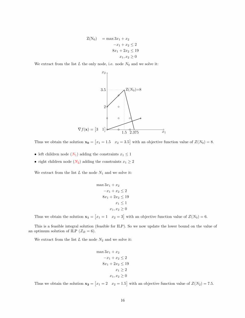
Z(N0) = max 3x1 + x2

−x1 + x2 ≤ 2

8x1 + 2x2 ≤ 19

x1, x2 ≥ 0

We extract from the list L the only node, i.e. node N0 and we solve it:

x1

x2

Z(N0)=83.5

2

1.5 2.375∇f(x) =

[3 1

]Thus we obtain the solution x0 =

[x1 = 1.5 x2 = 3.5





max 3x1 + x2

−x1 + x2 ≤ 2

8x1 + 2x2 ≤ 19

x1 ≤ 1

x1, x2 ≥ 0

Thus we obtain the solution x1 =[x1 = 1 x2 = 3




max 3x1 + x2

−x1 + x2 ≤ 2

8x1 + 2x2 ≤ 19

x1 ≥ 2

x1, x2 ≥ 0

Thus we obtain the solution x2 =[x1 = 2 x2 = 1.5


16

Z(N1)=6

x1

x2

3

1∇f(x) =

[3 1

]

Z(N2)=7.5

x1

x2

1.5

2∇f(x) =

[3 1

]2.375




max 3x1 + x2

−x1 + x2 ≤ 2

8x1 + 2x2 ≤ 19

x1 ≥ 2

x2 ≤ 1

x1, x2 ≥ 0

Z(N3)=7.375

x1

x2

1

∇f(x) =[3 1

]2.3752.125

Thus we obtain the solution x3 =[x1 = 2.125 x2 = 1





17

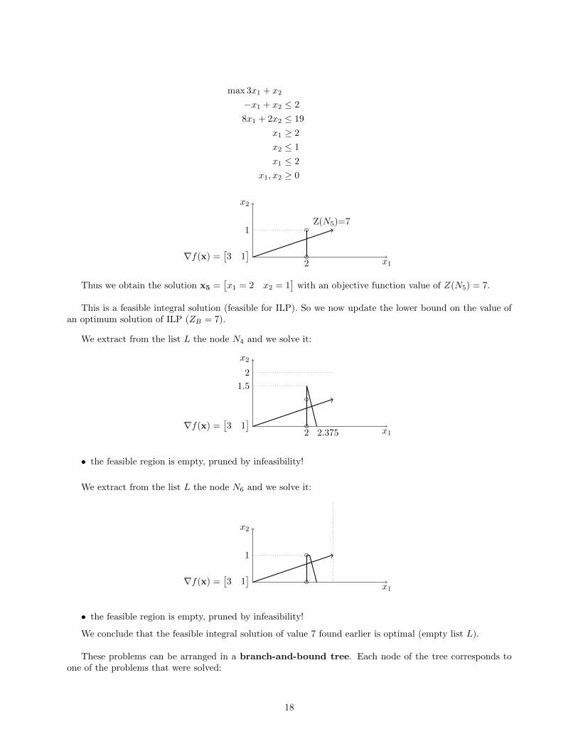
max 3x1 + x2

−x1 + x2 ≤ 2

8x1 + 2x2 ≤ 19

x1 ≥ 2

x2 ≤ 1

x1 ≤ 2

x1, x2 ≥ 0

Z(N5)=7

x1

x2

1

∇f(x) =[3 1

]2

Thus we obtain the solution x5 =[x1 = 2 x2 = 1




x1

x2

2

1.5

2∇f(x) =

[3 1

]2.375

• the feasible region is empty, pruned by infeasibility!


x1

x2

1

∇f(x) =[3 1

]• the feasible region is empty, pruned by infeasibility!

We conclude that the feasible integral solution of value 7 found earlier is optimal (empty list L).

These problems can be arranged in a branch-and-bound tree. Each node of the tree corresponds toone of the problems that were solved:

18

Figure 2: B&B tree of example 2

1.6 Minimization of concave piece-wise affine functions

• Consider an minimization model with an objective function given by the sum of concave piece wiseaffine functions

∑nj=1 f

j(xj), where each f j(xj) has a kj-piecewise description

• Similar results can be derived for a maximization of a convex piece-wise affine functions

f j(xj) = f ji (xj) if αji−1 ≤ xj ≤ α

ji i = 1, . . . , kj

Example: consider the variable x1 and k = 3, α0 = 0, α1 = 20, α2 = 40, α3 = 50

f1(x1) =

54x1 if 0 ≤ x1 ≤ 20

0.5x1 + 15 if 20 ≤ x1 ≤ 40

0.125x1 + 30 if 40 ≤ x1 ≤ 50

19

x

f(x)

25

3536.25

20 40 50

the optimization model reads as follows:

Z(LP)= min

n∑j=1

f j(xj)

n∑j=1

aijxj ≥ bi i = 1, . . . ,m

xj ≥ 0 j = 1, . . . , n

Transformation into an ILP

• for each of the original variable and for each piece of its concave piece-wise affine function, we canintroduce a binary variable

vji ∈ {0, 1} (j = 1, . . . , n, i = 1, . . . , kj)

• we then add the following constrains to impose that only one piece of the piece-wise affine function isselected:

kj∑i=1

vji = 1 (j = 1, . . . , n)

• for each variable we can now introduce a set of continuous variables pji (i = 0, 1, . . . , kj) representing the

weights of the convex linear combination of the value αji (i = 0, 1, . . . , kj), then we add the constraints:

kj∑i=0

αjip

ji = xj j = 1, . . . , n

kj∑i=0

pji = 1 j = 1, . . . , n

20

• for each variable xj (j = 1, . . . , n) only a variable vji (j = 1, . . . , n, i = 1, . . . , kj) takes the value of 1and accordingly we should impose:

vj1 = 1⇒ pj0 + pj1 = 1

vj2 = 1⇒ pj1 + pj2 = 1

vj3 = 1⇒ pj2 + pj3 = 1

. . .

we then should add the constraints:

pji−1 + pji ≥ vji j = 1, . . . , n, i = 1, . . . , kj

• we can now rewrite the function f j(xj) (j = 1, . . . , n)

f j(xj) =

kj∑i=0

(f j(αji ))p

ji

• the equivalent ILP reads as follows:

Z(LP)= min

n∑j=1

kj∑i=0

(f j(αji ))p

ji

n∑j=1

aijxj ≥ bi i = 1, . . . ,m

kj∑i=1

vji = 1 j = 1, . . . , n

kj∑i=0

αjip

ji = xj j = 1, . . . , n

kj∑i=0

pji = 1 j = 1, . . . , n

pji−1 + pji ≥ vji j = 1, . . . , n, i = 1, . . . , kj

xj ≥ 0 j = 1, . . . , n

vji ∈ {0, 1} j = 1, . . . , n, i = 1, . . . , kj

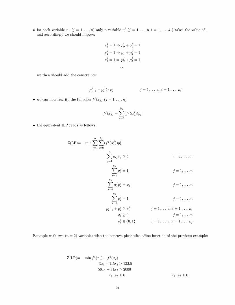
Example with two (n = 2) variables with the concave piece wise affine function of the previous example:

Z(LP)= min f1(x1) + f2(x2)

3x1 + 1.5x2 ≥ 132.5

50x1 + 31x2 ≥ 2000

x1, x2 ≥ 0 x1, x2 ≥ 0

21

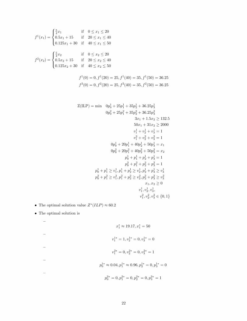
f1(x1) =

54x1 if 0 ≤ x1 ≤ 20

0.5x1 + 15 if 20 ≤ x1 ≤ 40

0.125x1 + 30 if 40 ≤ x1 ≤ 50

f2(x2) =

54x2 if 0 ≤ x2 ≤ 20

0.5x2 + 15 if 20 ≤ x2 ≤ 40

0.125x2 + 30 if 40 ≤ x2 ≤ 50

f1(0) = 0, f1(20) = 25, f1(40) = 35, f1(50) = 36.25

f2(0) = 0, f2(20) = 25, f2(40) = 35, f2(50) = 36.25

Z(ILP) = min 0p10 + 25p11 + 35p12 + 36.25p13

0p20 + 25p21 + 35p22 + 36.25p23

3x1 + 1.5x2 ≥ 132.5

50x1 + 31x2 ≥ 2000

v11 + v12 + v13 = 1

v21 + v22 + v23 = 1

0p10 + 20p11 + 40p12 + 50p13 = x1

0p20 + 20p21 + 40p22 + 50p23 = x2

p10 + p11 + p12 + p13 = 1

p20 + p21 + p22 + p23 = 1

p10 + p11 ≥ v11 , p11 + p12 ≥ v12 , p12 + p13 ≥ v13p20 + p21 ≥ v21 , p21 + p22 ≥ v22 , p22 + p23 ≥ v23

x1, x2 ≥ 0

v11 , v12 , v

13 ,

v21 , v22 , v

23 ∈ {0, 1}

• The optimal solution value Z∗(ILP ) ≈ 60.2

• The optimal solution is

–x∗1 ≈ 19.17, x∗1 = 50

–v1∗1 = 1, v1∗2 = 0, v1∗3 = 0

–v2∗1 = 0, v2∗2 = 0, v2∗3 = 1

–p1∗0 ≈ 0.04, p1∗1 ≈ 0.96, p1∗2 = 0, p1∗3 = 0

–p2∗0 = 0, p2∗1 = 0, p2∗2 = 0, p2∗3 = 1

22

1.7 Minimization of convex piece-wise affine functions

Let f(x) be a generic convex piece-wise affine function with a k-piecewise description

f(x) = fi(x) if αi−1 ≤ x ≤ αi i = 1, . . . , k

Affine Functions : fi(x) = ax+ b (fi(x+ y) = ax+ ay + b)

Example: k = 3, α0 = 0, α1 = 20, α2 = 40, α3 = 50, f2(20) = 10, f3(40) = 30

f(x) =

0.5x if 0 ≤ x ≤ 20

x− 10 if 20 ≤ x ≤ 40

2x− 50 if 40 ≤ x ≤ 50

x

f(x)

10

30

50

20 40 50

• Consider an minimization model with an objective function given by the sum of convex piece wise affinefunctions

∑nj=1 f

j(xj), where each f j(xj) has a kj-piecewise description

Consider the following LP optimization model (the variables can also be integer):

Z(LP)= min

n∑j=1

f j(xj)

n∑j=1

aijxj ≥ bi i = 1, . . . ,m

xj ≥ 0 j = 1, . . . , n

23

Transformation into an LP

for each original variable we can introduce a new variable yj (j = 1, ,n) and modify the objectivefunction and the constraints as follows:

Z(LP)= min

n∑j=1

yj

yj ≥ f ji (xj) j = 1, . . . , n, i = 1, . . . , kjn∑

j=1

aijxj ≥ bi i = 1, . . . ,m

xj ≥ 0 j = 1, . . . , n

Example with two (n = 2) variables with the convex piece wise affine function of the previous example:

Z(LP) = min f1(x1) + f2(x1)50x1 + 31x2 ≥ 250−3x1 + 2x2 ≥ 4x1, x2 ≥ 0

f1(x1) =

f11 (x1) = 0.5x1 if 0 ≤ x1 ≤ 20

f12 (x1) = x1 − 10 if 20 ≤ x1 ≤ 40

f13 (x1) = 2x1 − 50 if 40 ≤ x1 ≤ 50

f2(x2) =

f21 (x2) = 0.5x2 if 0 ≤ x2 ≤ 20

f22 (x2) = x2 − 10 if 20 ≤ x2 ≤ 40

f23 (x2) = 2x2 − 50 if 40 ≤ x2 ≤ 50

Z(LP) = min y1 + y2

y1 ≥ 0.5x1

y1 ≥ x1 − 10

y1 ≥ 2x1 − 50

y2 ≥ 0.5x2

y2 ≥ x2 − 10

y2 ≥ 2x2 − 50

50x1 + 31x2 ≥ 250

−3x1 + 2x2 ≥ 4

x1, x2, y1, y2 ≥ 0

– the optimal solution value is Z(LP)=≈ 3.4352

– the optimal solution is: x∗ =

[≈ 1.95

≈ 4.92

]y∗ =

[≈ 0.97

≈ 2.46

]

24

1.8 Constraints with absolute value expressions

• consider the following constraint

|n∑

j=1

ajxj | ≥ b

(where b > 0)

{∑nj=1 ajxj ≥ b if

∑nj=1 ajxj ≥ 0∑n

j=1 ajxj ≤ −b if∑n

j=1 ajxj < 0

• The feasible regions of the two constraint are disjointed. We can then linearize this constraint intro-ducing a binary variable v. We then get:

n∑j=1

ajxj ≥ b−Mv (23)

n∑j=1

ajxj ≤ −b+M(1− v) (24)

xj ≥ 0 j = 1, . . . , n (25)

v ∈ {0, 1} (26)

• M is called Big-M value and it is a “very” large constant

example:

| − 2x1 + x2| ≥ 2

x1

x2

−4

2

4

−2

−2x1 + x2 = 0

x1

x2

−2x1 + x2 = −1−2x1 + x2 = 1

25

x1

x2

1

2

32

6

4

−2x1 + x2 ≥ 2

−2x1 + x2 ≤ −2

We linearize the constraint as follow:

−2x1 + x2 ≥ 2−Mv

−2x1 + x2 ≤ −2 +M(1− v)

x1, x2 ≥ 0

v ∈ {0, 1}

• consider the following constraint

|n∑

j=1

ajxj | ≤ b

(where b > 0); then it is sufficient to impose two linear constraints:

n∑j=1

ajxj ≤ b (27)

n∑j=1

ajxj ≥ −b (28)

1.9 Minimization of objective functions with absolute values

• consider the following objective function in form of minimization with absolute values:

min

n∑j=1

|cjxj − dj | (29)

n∑j=1

aijxj ≥ bi i = 1, . . . ,m (30)

xj ≥ 0 j = 1, . . . , n (31)

• for each of the variable we introduce an addition continuous variable zj and we obtain:

26

min

n∑j=1

zj (32)

zj ≥ cjxj − dj j = 1, . . . , n (33)

zj ≥ −cjxj + dj j = 1, . . . , n (34)n∑

j=1

aijxj ≥ bi i = 1, . . . ,m (35)

xj ≥ 0 j = 1, . . . , n (36)

• the same transformation works in case of integer variables xj

1.10 Soft Constraints, Big-M constraints, Alldiff constraints

Soft Constraints

• Consider the following “hard” constraint

n∑j=1

ajxj ≥ b

• All the solutions∑n

j=1 ajxj < b are discarded.

• In addition this constraint can lead to an empty feasible region, for example:

2x1 + 4x2 ≥ 10

x1, x2 ∈ {0, 1}

• the constraint can be relaxed adding a continuous non-negative variable u:

n∑j=1

aixj + u ≥ b

• then the variable u, which represents the violation of the constraint, can be minimized in the objectivefunction

• in case of equality constraints the corresponding soft constraint is:

n∑j=1

ajxj + u+ − u− = b

• where u+ and u− are two additional continuous variables.

Big-M constraints

• Consider a constraint:n∑

j=1

ajxj ≥ b

• this constraint has to be activated iff

27

– a binary variable u take the value of 1

n∑j=1

ajxj ≥ b−M(1− u)

– a binary variable u take the value of 0

n∑j=1

ajxj ≥ b−Mu

• the value of the binary variable u is driven by the other constraints of the model

• M is called Big-M and it is a constant large enough to relax the constraint

Alldiff constraints

• Let x and y two integer variables that must take different values. The ranges of the two variables are:{x ∈ [0,Mx]

y ∈ [0,My]

• the logical constraint is the following:

x 6= y ⇔ x ≥ y + 1 OR y ≥ x+ 1

• introducing a binary variable z we can write the following two Big-M linear constraints:

⇔

x ≥ y + 1− (My + 1)z

y ≥ x+ 1− (Mx + 1)(1− z)0 ≤ x ≤Mx

0 ≤ y ≤My

z ∈ {0, 1}

• in this case the Big-M values can be set to Mx + 1 and My + 1 respectively.

28

1.11 Boolean expressions using binary variables

• A Boolean expression, also called propositional logic formula, is built from

1) boolean-valued functions (also called proposition)

∗ functions f : X −→ B

∗ X is an arbitrary set

∗ B is a boolean domain B ∈ {TRUE, FALSE}– example: a function that returns TRUE if a number is even and FALSE otherwise, X ≡ Z+ andB ∈ {TRUE, FALSE}

– a boolean-valued functions can be represented by a binary variable:

x ∈ {0, 1}, if TRUE −→ x = 1, else (if FALSE) −→ x = 0

2) boolean operators:

∗ AND – conjunction – denoted also by ∧∗ OR – disjunction – denoted also by ∨

– the negation of a boolean-valued functions represented by a binary variable is NOT f , it correspondsto the binary variable (1− x)

3) parentheses

• A Boolean expression is said to be satisfiable if it can be made TRUE by assigning appropriate logicalvalues (i.e., TRUE, FALSE) to its binary variables

• Example of Boolean expression:

(xa OR xb) AND (xc OR xd) AND ( NOT xe)

• Conjunction:

xa AND xb ⇔

{xa ≥ 1

xb ≥ 1

• Disjunction:xa OR xb ⇔ xa + xb ≥ 1

• Remarque : the boolean operator AND come first than OR. xa OR xb AND xc is equivalent to xa OR (xb AND xc)

Conjunctive Normal Form (CNF)

• A Boolean expression is said to in Conjunctive Normal Form if it is expressed as conjunctions ofdisjunctions

• examples:

– xa AND xb

– (xa OR xb) AND xc

• Equivalences:

– NOT ( NOT xa) = xa

– NOT (xa OR xb) = ( NOT xa) AND ( NOT xb)

– NOT (xa AND xb) = ( NOT xa) OR ( NOT xb)

– xa AND (xb OR xc) = (xa AND xb) OR (xa AND xc)

– xa OR (xb AND xc) = (xa OR xb) AND (xa OR xc)

29

Transforming CNF into linear equations

• for each disjunction ( OR ) we have an inequality constraint ≥ 1

• for each conjunction ( AND ) the left hand side of the inequality is written replacing:

– OR with +

– each ( NOT xa) with (1− xa)

Logical Implications between binary variables

• xa ⇒ xb = ( NOT xa) OR xb

• this can be written using binary variables as follow:

(1− xa) + xb ≥ 1 (xb ≥ xa)

• Attention that xa ⇒ xb implies also NOT xb ⇒ NOT xa = ( NOT ( NOT xb)) OR NOT xa = ( NOT xa) OR xb

examples

(1) (xa AND xb)⇒ xc

NOT (xa AND xb) OR xc

( NOT xa) OR ( NOT xb) OR xc

(1− xa) + (1− xb) + xc ≥ 1

(xa + xb − xc ≤ 1)

(2) (xa OR xb)⇒ xc

NOT (xa OR xb) OR xc

(( NOT xa) AND ( NOT xb)) OR xc

(( NOT xa) OR (xc)) AND (( NOT xb) OR (xc)){1− xa + xc ≥ 1

1− xb + xc ≥ 1

(3) xa ⇒ (xb AND xc)

NOT (xa) OR (xb AND xc)

(( NOT xa) OR (xb)) AND (( NOT xa) OR (xc)){1− xa + xb ≥ 1

1− xa + xc ≥ 1

(4) xa ⇒ (xb OR xc)

NOT (xa) OR (xb OR xc)

1− xa + xb + xc ≥ 1

(xb + xc ≥ xa)

(5) xa AND ( NOT xb) AND xc ⇒ NOT xd

NOT (xa AND ( NOT xb) AND xc) OR ( NOT xd)

( NOT xa) OR xb OR ( NOT xc) OR ( NOT xd)

1− xa + xb + 1− xc + 1− xd ≥ 1

(xa − xb + xc + xd ≤ 2)

30

1.12 Lagrangian Relaxations

Problem P to relax: (purely binary problem, but results extend to ILP)

Z(P ) = max

n∑j=1

vjxj (37)

n∑j=1

aijxj ≤ bi i = 1, . . . ,m (38)

n∑j=1

dkjxj = ek k = 1, . . . , l (39)

xj ∈ {0, 1} j = 1, . . . , n (40)

or equivalently

Z(P ) = max v>x (41)

Ax ≤ b (42)

Dx = e (43)

x ∈ {0,1} (44)

(A) Inequalities

1. Select a set of inequalities constraints and add a non-negative term to the objective function:

max

n∑j=1

vjxj +

m∑i=1

ui(bi −n∑

j=1

aijxj) (45)

with ui ≥ 0, ∀i. Lagrangian multiplier (valid upper bound).

2. Eliminate the selected constraints. Lagrangian Relaxation:

Z(L(P,u)) =m∑i=1

uibi + maxn∑

j=1

vjxj (46)

n∑j=1

dkjxj = ek k = 1, . . . , l (47)

xj ∈ {0, 1} j = 1, . . . , n (48)

where vj = vj −∑m

i=1 uiaij (j = 1, ..., n).

• If the optimal solution x∗ to L(P ) is feasible for P then it is not necessarily optimal for P : it is optimalif the two objective functions have the same value, i.e., if

m∑i=1

ui(bi −n∑

j=1

aijxj) = 0

(⇐⇒ if, ∀ i, either ui is 0 or constraint i is tight)

31

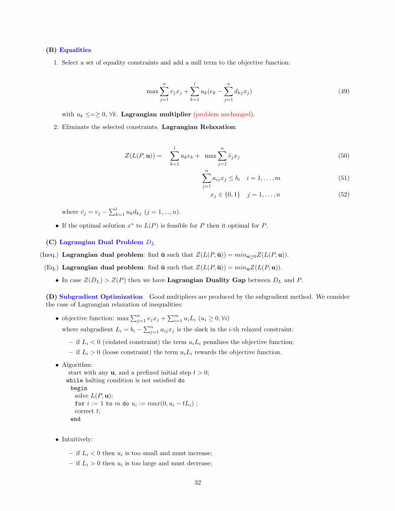
(B) Equalities

1. Select a set of equality constraints and add a null term to the objective function:

max

n∑j=1

vjxj +

l∑k=1

uk(ek −n∑

j=1

dkjxj) (49)

with uk ≤=≥ 0, ∀k. Lagrangian multiplier (problem unchanged).

2. Eliminate the selected constraints. Lagrangian Relaxation:

Z(L(P,u)) =

l∑k=1

ukek + max

n∑j=1

vjxj (50)

n∑j=1

aijxj ≤ bi i = 1, . . . ,m (51)

xj ∈ {0, 1} j = 1, . . . , n (52)

where vj = vj −∑l

k=1 ukdkj (j = 1, ..., n).

• If the optimal solution x∗ to L(P ) is feasible for P then it optimal for P .

(C) Lagrangian Dual Problem DL

(Ineq.) Lagrangian dual problem: find u such that Z(L(P, u)) = minu≥0Z(L(P,u)).

(Eq.) Lagrangian dual problem: find u such that Z(L(P, u)) = minuZ(L(P,u)).

• In case Z(DL) > Z(P ) then we have Lagrangian Duality Gap between DL and P .

(D) Subgradient Optimization Good multipliers are produced by the subgradient method. We considerthe case of Lagrangian relaxation of inequalities:

• objective function: max∑n

j=1 vjxj +∑m

i=1 uiLi (ui ≥ 0,∀i)

where subgradient Li = bi −∑n

j=1 aijxj is the slack in the i-th relaxed constraint:

– if Li < 0 (violated constraint) the term uiLi penalizes the objective function;

– if Li > 0 (loose constraint) the term uiLi rewards the objective function.

• Algorithm:start with any u, and a prefixed initial step t > 0;while halting condition is not satisfied do

begin

solve L(P,u);for i := 1 to m do ui := max(0, ui − tLi) ;correct t;

end

• Intuitively:

– if Li < 0 then ui is too small and must increase;

– if Li > 0 then ui is too large and must decrease;

32

– if Li = 0 then ui is fine (optimality condition).

• Standard formula for the step updating:

t = ϑZ(L(P,u))− Z∑m

i=1 L2i

where

– Z = incumbent solution value;

– ϑ decreases with the number of iterations, e.g.,: start with ϑ = 2; halve ϑ after some iterationswith no improvement.

• Two halting conditions:

– ∀ i, either (Li = 0) or (Li > 0 and ui = 0) (optimal multipliers);

– maximum number of iterations reached.

• Non-monotone method: the best u value is stored.

Different possible kinds of relaxation

• F (P ) = feasible region of P

• Fr(P ) = feasible region of the relaxation r of P

Figure 3: unfeasible solution Figure 4: feasible and optimal solution

Figure 5: Lagrangian Relaxation of Equalities

•

•

33

Figure 6: unfeasible solution

Figure 7: feasible non optimal solution

Figure 8: feasible and optimal solution

Figure 9: Lagrangian Relaxation of Inequalities

2 Capacitated Lot-Sizing problems

• One resource

• P products (i = 1, 2, . . . , n = |P |)

• T time periods (t = 1, 2, . . . ,m = |T |)

• dit demand of product i ∈ P in period t ∈ T

• capt capacity (time) in period t ∈ T

• capacity consumption

– vtit variable production time for product i ∈ P at t ∈ T

• costs

– hcit holding cost of product i ∈ P in t ∈ T

34

– fci cost for initial inventory for product i ∈ P– vcit variable production cost of product of i ∈ P in t ∈ T

Decision Variables (continuous variables) For each product i ∈ N and time period t ∈ T :

• xit = amount of production of product i in period t

• sit = inventory quantity of product i at the end of period t

• sii = amount of initial inventory of product i

min∑i∈P

fcisii +∑i∈P

∑t∈T

(vcitxit + hcitsit) (53)

sii + xi1 = di1 + si1 i ∈ P (54)

sit−1 + xit = dit + sit i ∈ P, t ∈ T \ {1} (55)∑i∈P

vtitxit ≤ capt t ∈ T (56)

xit, sit ≥ 0 i ∈ N, t ∈ T (57)

sii ≥ 0 i ∈ N (58)

• Constraints (55) are product flow balancing constraints. They impose to satisfy the demand of producti in period t using:

– production in period t

– the inventory at the end of period t− 1

– if sit−1 + xit ≥ dit, this extra quantity becomes the inventory at the end of period t

• Constraints (54) balance the flow of the first period using the initial inventory

• Constraints (56) are machine capacity constraints. They impose that the production time does notexceed the maximum time capacity of the resource for each period.

Example

• 2 products n = 2, i = 1, i = 2

• for product 1

period 1 2 3d1t 100 200 10vt1t 20 10 10hc1t 110 100 100vc1t 1100 1000 1000

• for product 2

• 3 time periods m = 3, t = 1, t = 2, t = 3

• available capacities cap1 = 2500, cap2 = 2100, cap3 = 2500:

• initial cost fc1 = 3000, fc2 = 3000

35

period 1 2 3d2t 10 100 150vt2t 10 5 5hc2t 105 105 105vc2t 900 800 800

min 1100x11 + 1000x12 + 1000x13+

900x21 + 800x22 + 800x23+

110s11 + 100s12 + 100s13+

120s21 + 110s22 + 110s23+

3000si1 + 3000si2

x11 + si1 = 100 + s11

x21 + si2 = 10 + s21

x12 + s11 = 200 + s12

x13 + s12 = 10 + s13

x22 + s21 = 100 + s22

x23 + s22 = 150 + s23

20x11 + 10x21≤2500

10x12 + 5x22≤2100

10x13 + 5x23≤2500

si1, si2,

x11, x12, x13,

x21, x22, x23,

s11, s12, s13,

s21, s22, s23 ≥ 0

• The optimal solution value Z∗(LP ) = 575400.00

• The optimal solution is

x∗11 = 120, x∗12 = 160, x∗13 = 10

x∗21 = 10, x∗22 = 100, x∗23 = 150

s∗11 = 40, s∗12 = 0, s∗13 = 0

s∗21 = 0, s∗22 = 0, s∗23 = 0

si∗1 = 20, si∗2 = 0

36

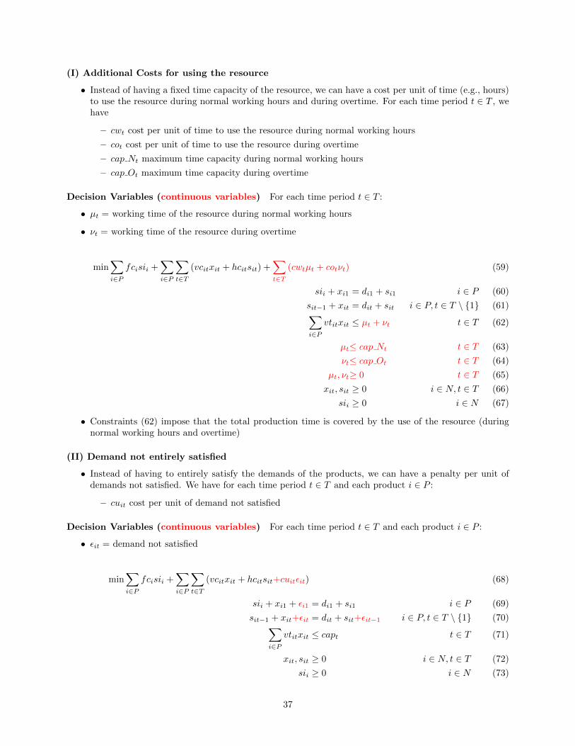
(I) Additional Costs for using the resource

• Instead of having a fixed time capacity of the resource, we can have a cost per unit of time (e.g., hours)to use the resource during normal working hours and during overtime. For each time period t ∈ T , wehave

– cwt cost per unit of time to use the resource during normal working hours

– cot cost per unit of time to use the resource during overtime

– cap Nt maximum time capacity during normal working hours

– cap Ot maximum time capacity during overtime

Decision Variables (continuous variables) For each time period t ∈ T :

• µt = working time of the resource during normal working hours

• νt = working time of the resource during overtime

min∑i∈P

fcisii +∑i∈P

∑t∈T

(vcitxit + hcitsit) +∑t∈T

(cwtµt + cotνt) (59)

sii + xi1 = di1 + si1 i ∈ P (60)

sit−1 + xit = dit + sit i ∈ P, t ∈ T \ {1} (61)∑i∈P

vtitxit ≤ µt + νt t ∈ T (62)

µt≤ cap Nt t ∈ T (63)

νt≤ cap Ot t ∈ T (64)

µt, νt≥ 0 t ∈ T (65)

xit, sit ≥ 0 i ∈ N, t ∈ T (66)

sii ≥ 0 i ∈ N (67)

• Constraints (62) impose that the total production time is covered by the use of the resource (duringnormal working hours and overtime)

(II) Demand not entirely satisfied

• Instead of having to entirely satisfy the demands of the products, we can have a penalty per unit ofdemands not satisfied. We have for each time period t ∈ T and each product i ∈ P :

– cuit cost per unit of demand not satisfied

Decision Variables (continuous variables) For each time period t ∈ T and each product i ∈ P :

• εit = demand not satisfied

min∑i∈P

fcisii +∑i∈P

∑t∈T

(vcitxit + hcitsit+cuitεit) (68)

sii + xi1 + εi1 = di1 + si1 i ∈ P (69)

sit−1 + xit+εit = dit + sit+εit−1 i ∈ P, t ∈ T \ {1} (70)∑i∈P

vtitxit ≤ capt t ∈ T (71)

xit, sit ≥ 0 i ∈ N, t ∈ T (72)

sii ≥ 0 i ∈ N (73)

37

• Constraints (70) are an extension of the previous flow constraints. They impose that the demand ofperiod t and the unsatisfied demand of period t − 1 (i.e., εit−1) should be satisfied. The request forproduction can be then decreased by the unsatisfied demand of period t (i.e., εit)

2.1 Capacitated Lot-Sizing problems with setups

• In case of production of a product i ∈ P in period t ∈ T typically a setup time and a setup cost arerequired.

• capacity consumption

– stit setup time of product i ∈ P in period t ∈ T

• costs

– scit setup cost of product i ∈ P in period t ∈ T

Decision Variables (binary variables) For each product i ∈ N and time period t ∈ T :

• yit =

{1 if there is a setup for product i in t0 otherwise

• A link is necessary between the decision variable of production quantities (xit – continuous variables)and the variables modelling the setup (yit – binary variables)

Big-M values

• we need a upper bound on the maximum production of a specific product i considering the time periodsfrom t to k (k ≥ t):

sditk =

k∑j=t

dij

this quantity represents the sum of the demand of product i from period t to period k

• a first Big-M value is then sditm

• small Big-M value better model the link between the variables and increases the quality of the linearprogramming relaxation of the model.

• an other possible upper bound on the maximum production is given by

(capt − stit)vtit

where capt − stit represents an upper bound of the maximum time which can be used to produce aproduct i. Once divided by vtit (the production time per unit of product), we obtain an other validupper bound on the production quantity of i.

• the best Big-M is then the minimum among the two:

Big Mit = min{(capt − stit)/vtit, sditm}

38

2.1.1 Formulation 1

min∑i∈P

fcisii +∑i∈P

∑t∈T

(scityit + vcitxit + hcitsit) (74)

sii + xi1 = di1 + si1 i ∈ P (75)

sit−1 + xit = dit + sit i ∈ P, t ∈ T \ {1} (76)

Big Mit · yit≥ xit i ∈ P, t ∈ T (77)∑i∈P

(stityit + vtitxit) ≤ capt t ∈ T (78)

xit, sit ≥ 0 i ∈ P, t ∈ T (79)

sii ≥ 0 i ∈ P (80)

yit∈ {0, 1} i ∈ P, t ∈ T (81)

Example of linking constraints

• the setup times are

period 1 2 3st1t 100 100 100st2t 110 110 110

• The Big-M values for the previous examples are:

• sd113 = 310, sd123 = 210, sd133 = 10

• sd213 = 260, sd223 = 250, sd233 = 150

• (cap1 − st11)/vt11) = 120, (cap2 − st12)/vt12) = 200, (cap3 − st13)/vt13) = 240

• (cap1 − st21)/vt21) = 239, (cap2 − st22)/vt22) = 398, (cap3 − st23)/vt23) = 478

• these are the additional constraints:

x11 ≤ 120y11, x12 ≤ 200y12, x13 ≤ 10y13

x21 ≤ 239y21, x22 ≤ 250y22, x23 ≤ 150y23

2.1.2 Formulation 2

Decision Variables (continuous variables)

• For each product i ∈ P and time periods t ∈ T and k ∈ T, k ≥ t:

• zvitk = fraction of production plan for product i where production in period t satisfies demand fromperiod t to period k

• For each product i ∈ P and time periods t ∈ T :

• wit = fraction of the initial inventory plan for product i where demand is satisfied for the first t periods

• To build the model we compute the following quantities:

cvitk = vcit · sditk +

k∑s=t+1

s−1∑u=t

hciudis

total production and holding cost for producing product i in period t to satisfy demand for the periodst until k. Attention: only summation with k ≥ t+ 1 and s− 1 ≥ t are considered.

39

•

ciit = fcisdi1t +

t∑s=2

s−1∑u=1

hciudis

total production and holding cost for initial inventory for product i to satisfy demand from period 1up to period t. Attention: only summation with t ≥ 2 and s− 1 ≥ 1 are considered.

min∑i∈P

∑t∈T

(scityit + ciitwit) +∑i∈P

∑t∈T

m∑k=t

cvitkzvitk (82)∑k∈T

(wik + zvi1k) = 1 i ∈ P (83)

wit−1 +

t−1∑k=1

zvikt−1 =

m∑k=t

zvitk ∀i ∈ N, t ∈ T \ {1} (84)

m∑k=t

zvitk ≤ yit i ∈ P, t ∈ T (85)

∑i∈P

stityit +∑i∈P

m∑k=t

vtitsditkzvitk ≤ capt t ∈ T (86)

wit ≥ 0 i ∈ P, t ∈ T (87)

zvitk ≥ 0 i ∈ P, t, k ∈ T, k ≥ t (88)

yit ∈ {0, 1} i ∈ P, t ∈ T (89)

• Constraints (83) and (84) allow to satisfy the demands.

• Constraints (83) impose that a flow of 1 unit is set out of the first node.

• Take the example and consider that the initial inventory is not used, i.e., all w variables are set to 0.Examples of feasible solutions for the product 1 are:

* zv111 = 1, it means that all the demand of the product 1 in period 1 is satisfied by the productionin period 1 and the associated cost is cv111 = vc11 · sd111 = 100 · 1100 = 110000

* zv113 = 1, it means that all the demands of the product 1 in periods 1, 2 and 3 are satisfied bythe production in period 1 and the associated cost is cv113 = vc11 · sd113 + d12 · hc11 + d12 · hc12 =310 · 1100 + 200 · 110 + 10 · 100 = 341000 + 24100 = 365100

* combinations that sum up to 1, e.g., zv111 = 0.5 and zv113 = 0.5. This means that only half ofthe demands of the product 1 in periods 2 and 3 are satisfied by the production in period 1 (andthe corresponding cost is paid).

• Constraints (84) assure that the demands of nodes t ∈ T \{1} are also satisfied. They force that if partof the flow ends before a specific node than it must be compensated by additional flow emanating fromit. Remember that the part of the flow which overtakes a node contribute to the demand of the nodeas well (see the definition of the variable). For example:

* if zv111 = 1, then zv122 + zv123 = 1

• Constraints (85) forces the setups in case of production.

• Constraints (86) makes sure that the capacity is respected.

40

t = 1start t = 2 t = 3

w12

w13

w11

zv111

zv112

zv113zv122

zv123

zv133

Figure 10: Network for the example and product i = 1.

3 Scheduling of jobs

Notation

• Scheduling systems are characterized by different elements:

- machines (processors) or resources

- configurations and features of the machines

- level of automation

- handling systems

- . . .

• We denote generically a machine a resource (e.g., a computer, an operator, a department, a productiondivision . . . )

• The machines executes jobs which can consist in a single operation or in a series of operations thatcompose a productive process (cycle of production).

• The specific characteristics of the machines, of jobs and the objective function determine the nature ofthe the scheduling problems (a large family of optimization problems).

1) Principal Input Data

• Processing time (pij): execution time of job j on machine i.

* pj if the execution time does not depend on the machine

* if a job is composed by multiple operations, we denote by pzj the execution time of operation z ofjob j

• Release date (rj): earlies time in which a job j can start

• Due date (dj): time in which job j is expected to end. Sub-cases:

* sometime this corresponds to a maximum deadline which must be respected.

* in some other cases a job can end with a delay with respect to the due date.

• Setup time (sjk): time to prepare the machine to change from job j to job k (in general it depends toa couple of job but it can be fixed, i.e. it can linked to the machine only: si)

• Precedences k ≺ j (k precedes j): this indicates that the job j can start only after the job k is finished

41

2) Scheduling Decisions

• Completion time (Czj): instant of time in which the operation z of job j terminates (Cj in case of asingle operation)

• Starting time (Szj): instant of time in which the operation z of job j starts (Sj in case of a singleoperation)

• In general Szj = Czj − pzj , so only one of the two decisions is indeed necessary

3) Different objective functions

Objective functions based on the completions time of the jobs (Cj)

• Makespan: Cmax = maxj(Cj)

– completion time of the last job

– it determines the total time necessary for the execution of all jobs

– it is one of the most common objective function

• Transit time∑n

j=1 Cj

– it is used as an indicator of the Work-in-Process costs (since it measure the jobs waiting to beprocessed)

• Weighted Transit time∑n

j=1 wjCj

– Like the Transit time but the each job has a different monetary value

Other objective functions based on delays

• these quantities measure the delay of the jobs

Lj = Cj − dj Lateness (it can be positive or negative)Tj = max(0, Cj − dj) Tardiness (delay in delivery)Ej = max(0, dj − Cj) Earliness (advance in delivery)

• As for the completion time, we can minimize the maximum or the sum or the weighted sum

Lmax = maxj(Lj)∑n

j=1 Lj

∑nj=1 wjLj

Tmax = maxj(Tj)∑n

j=1 Tj∑n

j=1 wjTjEmax = maxj(Ej)

∑nj=1Ej

∑nj=1 wjEj

• for Just in Time, you can minimize both the delay and the advance in delivery:

Jj = Ej + TjJmax = maxj(Jj)

∑nj=1 Jj

∑nj=1 wjJj

42

3.1 Solution techniques

• principal methods (heuristic and exact):

– Dispatching rule (constructive heuristics)

– Metaheuristic

– Branch-and-Bound

– Dynamic Programming

– Constraint programming

– Mathematical Programming

– . . .

3.2 Dispatching rules

• The idea is to order the jobs (ordering rules)

• Two are the main categories of Dispatching rules in function of the ordering of jobs

– static rules: the priority of the jobs is defined only once at the beginning of the algorithm

– dynamic rules : the priority of the jobs changes during the execution of the algorithm

• In function of the way the solution is built, we have two typologies of algorithms

– Sequential algorithm : assign one job at a time

– Parallel algorithm : select a subset of jobs and try to assign them altogether

Principal Ordering rules

ERD Earliest Release Date, equivalent to F.I.F.O. (first in first out)

LPT Longest Processing Time, decreasing order of processing time

SPT Shortest Processing Time, increasing order of processing time

WSPT Weighted Shortest Processing Time, increasing order of ratio between processing time and priorityof the job

EDD Earliest Due Date, increasing order of due-date (or deadline)

SST Shortest Setup Time, increasing order of setup

Rule data objective of the ruleERD rj makespanEDD dj Lmax

LPT pj balancing of identical machines,makespan

SPT pj average completion timeWSPT pj , wj weighted completion timeSST setup average completion time,

makespan

• These rules normally produce heuristic solutions

43

3.3 Classification of Scheduling problems

• A three field classification is used:α|β|γ

α = (α1α2) features of the machines

α1 ∈ {∅, P,Q,R, PMPM,QMPM,G,X,O, F, J}α2 ∈ {∅,numero}

β = features of the jobs (β1, β2, β3, β4, β5, β6)

β1 : preemption

β2 : precedences

β3 : release time

β4 : features of processing times

β5 : deadline

β6 : batch

γ = objective function

given a function fj , γ is of the kind fmax,∑fj , or

∑wjfj

• a batch refers to multiple operations which can be executed on different machines

– P ||Cmax = parallel machine, makespan minimization

– P |prec|Cmax = identical parallel machines, generic precedence between jobs, makespan minimiza-tion

– 1|rj |Lmax = single machine, release time, minimization of the maximum lateness

– J ||Cmax = Job shop, makespan minimization

– . . .

• more details on the classification can be found here http://www.informatik.uni-osnabrueck.de/

knust/class/

• For some special cases dispatching according to specific orderings computes optimal solutions:

1. 1||∑Cj for SPT (Smith’s rule)

2. 1||∑wjCj for WSPT (Smith’s ratio rule)

3. 1||Lmax for EDD (Jackson’s rule)

Main Scheduling problems categories

• The scheduling problems can be subdivided in two main categories

– problems on a single machine

– problems on parallel machines

44

http://www.informatik.uni-osnabrueck.de/knust/class/

http://www.informatik.uni-osnabrueck.de/knust/class/

3.4 Problems on a single machine

• Often complex production systems are modelled as a single machine

– for example when we have a machine which is the slowest one and it determines the performanceof the entire system

– to have a first approximation of the system (aggregation of different machines)

– . . .

• Specialized algorithms for single machine problems can be then used to solve more complex schedulingproblems.

• There are subclasses of scheduling problems on a single machine which can be easily solved in polynomialtime (they belong to the class P of problems)

• There are also subclasses of scheduling problems on a single machine which cannot be easily solvedin polynomial time (they belong to the class NP-hard of problems). For these problems, branch-and-bound algorithms or mathematical models are necessary to find optimal solutions.

Example.

– Assign the jobs to the machine in order to minimize the makespan, i.e. the total execution time(end of the last job). Each job j as a processing time (pj) and there are setup times sjk betweeneach couple of jobs (j and k).

– This problem requires to find the optimal permutation of jobs and it belongs to the class NP-hard(reduction from the TSP)

3.5 Problems on parallel machines

• For this class of problems, m machines are given to execute the jobs. Jobs consist normally of a singleoperation.

• The goal is to assign the jobs to the machines and to determine the starting time and the ending timeof each job.

-

0 50 100

M3

M2

M1

J4 J7 J8

J1 J5

J2 J3 J6

Typology of machines

• Identical machines (in this case the processing time is independent on the the machine, i.e., pj )

• Uniform machines (in this case the processing time of a job is given by the ratio between the standardprocessing time a job and the speed of the machine. The machine are similar but they have differentspeed).

• Uncorrelated machines (in this case the machines are completely different and the processing timedepend on the couple job-machine: i.e.: pij .)

45

3.6 Shop Problems

• The jobs are constituted by multiple operation to be executed on different machines.

• Noramally each operation of a job is assigned to a given machine.

• This is the most generic class of scheduling problem which allows to model complex production systems.

• There are three main classes of Shop Problems:

1) Open shop (no precedence among the operations)

M3

M2

M1

J1 J3 J2

J2 J4 J1

J3 J2 J4

Solution 1

M3

M2

M1

J2 J1 J3

J1 J2 J4

J2 J3 J4

Solution 2

2) Flow shop (each job has a sequence of m operations to be executed on the machines 1, 2, . . . ,m)

M3

M2

M1 J1 J3 J2 J4

J1 J3 J2 J4

J1 J3 J2 J4

3) Job shop (each job j has nj operations to be executed on the machines µ1, µ2, . . . , µnj)

Job nj µ1 µ2 µ3 µ4

J1 3 1 2 4J2 4 2 1 3 4J3 3 3 2 4J4 2 3 1

M4

M3

M2

M1 J1 J2 J4

J1J2 J3

J3 J4 J2

J1J3 J2

46

Example: P |prec|Cmax

• Ordering: LPT (Longest Processing Time)

• 6 jobs, 2 identical parallel machines

• processing time pj = (40, 40, 30, 40, 70, 20)

• precedences:

• Sequential algorithm:Order: J5 J1 J2 J4 J3 J6

-

0 50 100

M2

M1 J5 J4

J1 J2 J3 J6

47

4 Job assignment to machines with ILP models

4.1 Production plans with precedence constraints

• We study the production plan of a machine available C hours a day

• We are given n jobs, each of which requires an processing time of pj hours (j = 1, . . . , n)

• We are given an upper bound m on the maximum number of days necessary to execute all the jobs (seethe exercise to find good upper bounds)

• We problem asks for determining the minimum number of days necessary to execute all the jobs.

Decision Variables (binary variables) For each job j = 1, . . . , n and for each day t = 1, . . . ,m:

• xtj =

{1 if the machine executes job j in day t0 otherwise

• yt =

{1 if the machine is used during day t0 otherwise

min

m∑t=1

yi (90)

m∑t=1

xtj = 1 j = 1 . . . , n (91)

n∑j=1

pjxtj ≤ Cyt t = 1 . . . ,m (92)

xtj ∈ {0, 1} j = 1 . . . , n, t = 1 . . . ,m (93)

yt ∈ {0, 1} t = 1 . . . ,m (94)

• The upper bound m can also be determined by a feasible assignment of the jobs, i.e. the number ofdays in a heuristic solutions. The smaller the value of m is the smaller is the size of the model, sinceit determines the number of decision variables.

Precedence constraints among jobs

• If the jobs have to be executed all of one piece, usually we have to respect a series of precedence betweenthe jobs.

• We study the case of assembly lines.

• We use the notation k ≺ j (k precedes j) in case the job j can start only after the end of job k

• The complete set of precedences is then provided as a assembly scheme and it is mathematicallyrepresented by a directed acyclic graph G = (V,A), where the vertices represent the jobs and the arcsrepresent the precedences:

A = {(k, j) : k ≺ j}

(A) simple precedences:

48

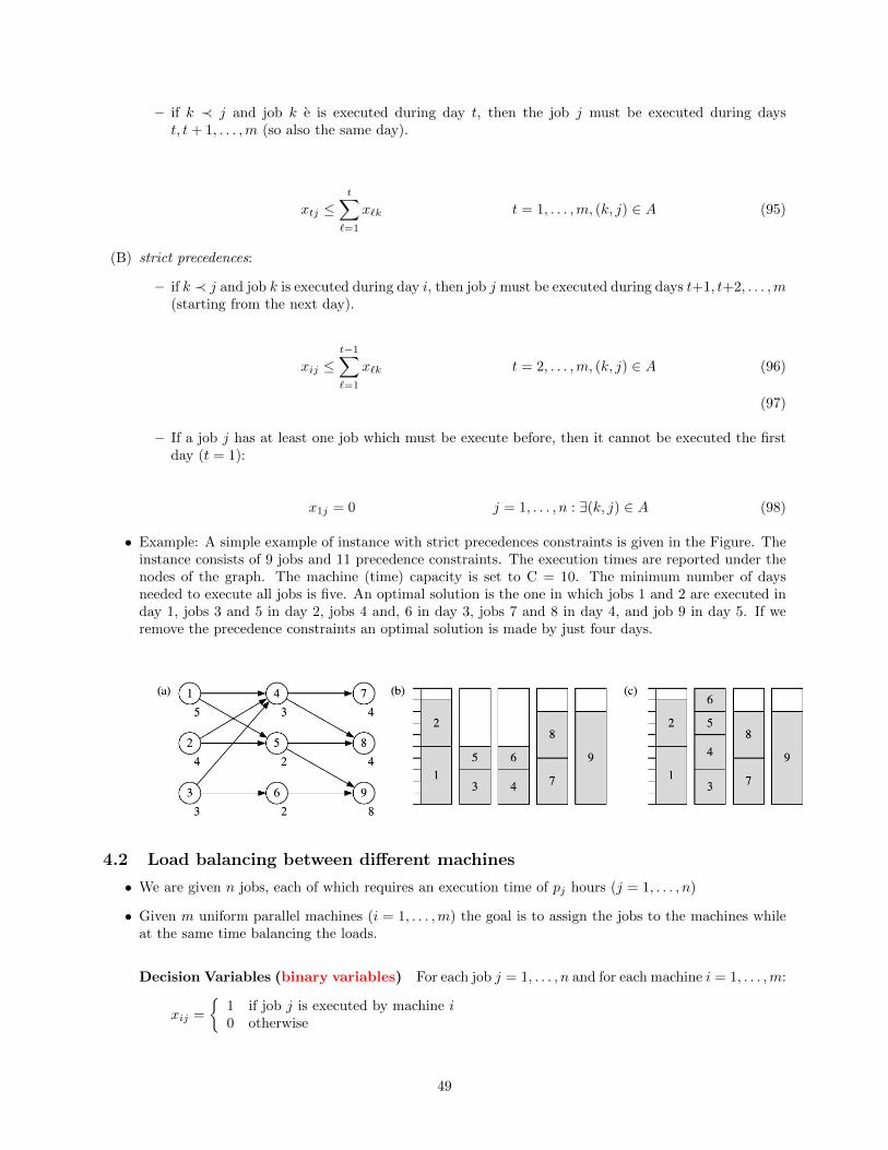
– if k ≺ j and job k e is executed during day t, then the job j must be executed during dayst, t+ 1, . . . ,m (so also the same day).

xtj ≤t∑

`=1

x`k t = 1, . . . ,m, (k, j) ∈ A (95)

(B) strict precedences:

– if k ≺ j and job k is executed during day i, then job j must be executed during days t+1, t+2, . . . ,m(starting from the next day).

xij ≤t−1∑`=1

x`k t = 2, . . . ,m, (k, j) ∈ A (96)

(97)

– If a job j has at least one job which must be execute before, then it cannot be executed the firstday (t = 1):

x1j = 0 j = 1, . . . , n : ∃(k, j) ∈ A (98)

• Example: A simple example of instance with strict precedences constraints is given in the Figure. Theinstance consists of 9 jobs and 11 precedence constraints. The execution times are reported under thenodes of the graph. The machine (time) capacity is set to C = 10. The minimum number of daysneeded to execute all jobs is five. An optimal solution is the one in which jobs 1 and 2 are executed inday 1, jobs 3 and 5 in day 2, jobs 4 and, 6 in day 3, jobs 7 and 8 in day 4, and job 9 in day 5. If weremove the precedence constraints an optimal solution is made by just four days.

4.2 Load balancing between different machines

• We are given n jobs, each of which requires an execution time of pj hours (j = 1, . . . , n)

• Given m uniform parallel machines (i = 1, . . . ,m) the goal is to assign the jobs to the machines whileat the same time balancing the loads.

Decision Variables (binary variables) For each job j = 1, . . . , n and for each machine i = 1, . . . ,m:

xij =

{1 if job j is executed by machine i0 otherwise

49

(A) The first possible objective function is to minimize the deviation from the mean value of the workloadcalled in the following:

µ =

∑nj=1 pj

m

• The load a of a machine i can be computed as follows:

Ci =

n∑j=1

pjxij

.

• Accordingly the objective function becomes:

min

m∑i=1

|Ci − µ|

• Since the objective function is expressed by an absolute value it is necessary to linearize it, obtainingthe following ILP model:

min

q∑i=1

zi (99)

zi ≥ Ci − µ i = 1, . . . ,m (100)

zi ≥ µ− Ci i = 1, . . . ,m (101)q∑

i=1

xij = 1 j = 1 . . . , n (102)

zi ≥ 0 i = 1, . . . ,m (103)

xij ∈ {0, 1} i = 1 . . . ,m, j = 1 . . . , n (104)

(B) The second possible objective function is to minimize the makespan Cmax, i.e., the total length of theschedule or, equivalently, the end of the the last job.

• This problem is called in the literature parallel processor scheduling problem (P ||Cmax) and the corre-sponding ILP model reads as follows:

min zn∑

j=1

pjxij ≤ z i = 1 . . . ,m

m∑i=1

xij = 1 j = 1 . . . , n

xij ∈ {0, 1} i = 1 . . . ,m; j = 1 . . . , n

• To these model one can add several constraints which are typical operational constraint in productionplanning. For example:

50

• Additional Constraints 1. Given a set S of couple of jobs (k, j) that must be executed on the samemachine, we add the following constraints:

xik = xij i = 1, . . . ,m, (k, j) ∈ S

• Additional Constraints 2. Given a set D of couple of jobs (k, j) that must be executed differentmachines, we add the following constraints:

xik + xij ≤ 1 i = 1, . . . ,m, (k, j) ∈ D

4.3 Sequencing of jobs on a single machine

• On input we are given the set J = {1, 2, . . . , n} of jobs to be processed by a single machine.

• For each job j ∈ J , we have:

– rj the realise date

– dj the maximum acceptable delay

– wj the cost associated with one time unit of delay between the release date and starting time ofthe job

• For each ordered pair of jobs (j, k) ∈ J × J a set up time of sjk time units has to separate the startingtime of j and k

Decision Variables (continuous variables) For each job j ∈ J :

• zj = starting time of job j

• One possible gaol is to find a sequence of jobs, together with their starting times times zj for eachj ∈ J , so as to minimize the global weighted delay with respect to their release date, i.e. to minimizethe cost function: ∑

j∈Jwj(zj − rj)

• A job cannot start before its realize date, so zj − rj ≥ 0

First ILP formulation

Decision Variables (binary variables) For each couple of jobs (j, k) ∈ J × J :

• δjk =

{1 if job j is scheduled before job k in the sequence0 otherwise

min∑j∈J

wj(zj − rj) (105)

rj ≤ zj ≤ rj + dj j ∈ J (106)

δjk + δkj = 1 j, k ∈ J, j 6= k (107)

zk ≥ zj + sjk −M(1− δjk) j, k ∈ J, j 6= k (108)

δjk ∈ {0, 1} j, k ∈ J, j 6= k (109)

zj ≥ 0 j ∈ J (110)

51

• The objective function (105) aims at minimizing the total cost due to the weighted delay of the job inthe sequence.

• Constraints (106) ensure that the delay of each job j respects its lower and upper bounds,

• Constraints (107) ensure that either job j start before job k, or vice versa, for any two jobs j and k.

• Constraints (108) ensure that the minimum separation constraints between jobs are satisfied, where M(which denotes a large positive constant) may be replaced by sjk + dj .

Valid Inequalities: Constraints (108) may be strengthened by defining the sets

•S = {(j, k) | rj + dj < rk, j, k ∈ J, j 6= k}

The set S of jobs denotes the set of ordered pairs of jobs (j, k) where j cannot start after k withoutviolating the feasible time windows

•S′ = {(j, k) | rj + dj + Sjk > rk, (j, k) ∈ S}

The set S′ denotes the set of ordered pairs of jobs (j, k) ∈ S such that k may be delayed by j due tothe separation constraints.

•T = {(j, k) | rj + dj ≥ rk, rk + dk ≥ rj , j, k ∈ J, j 6= k}

The set T denotes the set of ordered pairs of jobs (j, k) for which there is the possibility of either jobstar before the other.

Constraints (108) may be replaced by constraints (111)–(113):

δjk = 1 (j, k) ∈ S (111)

zk ≥ zj + sjk (j, k) ∈ S′ (112)

zk ≥ zj + sjk −M(1− δjk) (j, k) ∈ T (113)

Second ILP formulation

Decision Variables (binary variables) For each couple of jobs (j, k) ∈ J × J :

• xjk =

{1 if job j is scheduled in position k in the sequence0 otherwise

Decision Variables (continuous variables) For each position k ∈ J :

• yk = starting time of job in position k

52

min∑j∈J

wj(zj − rj) (114)

∑k∈J

xjk = 1 j ∈ J (115)∑i∈J

xjk = 1 k ∈ J (116)

zj ≤ rj + dj j ∈ J (117)

zj ≥ yk +M(xjk − 1) k ∈ J, i ∈ J (118)

yk ≥∑j∈J

rjxjk k ∈ J (119)

yk ≥ yk−1 + suv(xuk−1 + xvk − 1) k ∈ J, u, v ∈ J, k 6= 1, u 6= v (120)

xjk ∈ {0, 1} j ∈ J, k ∈ J (121)

zj ≥ 0 j ∈ J (122)

yk ≥ 0 k ∈ J (123)

• the objective function (114) aims at minimizing the total cost due to the weighted delay of the jobs inthe sequence.

• Constraints (115) and (116) ensure, respectively, that each job is assigned to one position in the sequenceand that to each position in the sequence one job is assigned.

• Constraints (117) ensure that the delay of each job j respects its upper bound

• Constraints (118) impose that the starting time of a job is equal to the the starting time correspondingto a position if and only if the job is assigned to that specific position.

• Constraints (119) ensure that no jobs starts before its release date.

• Constraints (120) ensure that the minimum separation constraints between jobs are satisfied, whiletogether they ensure that zj ≥ rj .

Valid Inequalities: The formulation may be further strengthened by including the following inequalities:

yk ≥ yk−1 + minu,v∈J,u 6=v

suv k ∈ I, k 6= 1. (124)

53

5 Heuristic Algorithms

Families of heuristic algorithms

• Simulated Annealing (Kirkpatrik, Gelatt e Vecchi 1983)

• Tabu Search (Glover, 1986)

• Variable Neighborhood Search (Mladenovic, Labbe e Hansen 1990s)

• Ant Colony Optimization − ACO (Colorni, Dorigo e Maniezzo 1992)

• Algoritmi Genetici (Rechenberg 1973, Holland 1975)

• Scatter Search (Glover 1965)

• Path Relinking (Glover 1965)

• Greedy Randomized Adaptive Search Procedure − GRASP (Feo e Resende 1989)

• Guided Local Search − GLS (Voudouris and Tsang 1990s)

• Artificial Neural Networks (Hopfield e Tank 1985, Mc Culloch and Pitts 1922)

• Memetic Algorithms (Moscato 1989)

• . . .

Case study problem

• Traveling Salesman Problem (TSP): given a graph G = (V,A) with costs cij on the arcs (i, j) ∈ A, findan Hamiltonian Circuit (a circuit that visits every vertex exactly once) of minimum cost.

• Example: consider 4 cities represented by the following graph:

• the distance matrix is represented by the costs cij , i.e, the following symmetric matrix:

A B C DA 0 20 42 35B 20 0 30 34C 42 30 0 12D 35 34 12 0

• Possible solutions:

– the sequence ABCD has a cost of 97

– the sequence ABDC has a cost of 106

54

• Encoding of a solution using a vector of size |V |:

each cell can represent the vertex in the sequence

For example a tour which starts in A, then visit C and then visit B and finally D before going back toA can be encoded by:

–A C B D

• The TSP corresponds to the scheduling problem of jobs for a machine minimizing the makespan (endof the last job) where each job j as a processing time (pj) and there are setup times sjk between eachcouple of jobs (j and k). The total processing time is a constants, i.e., it does not depend on the orderof job.

Typical philosophy of the heuristic algorithms

• Many heuristic algorithms are based on iterative calls of:

– a constructive algorithm

– a local search algorithm

Constructive algorithms

• Constructive algorithm are ”good sense” rules to quickly make a solution to the problem. Oftenthe rule is construct a solution with a sequence of ”locally optimal” decisions based on some criteria(greedy algorithms).

• Example: the classical greedy algorithm for the TSP is to start from the a node and go to the nearestvertex and repeating until all vertices have been visited (Closest Neighbor).

• Such algorithms are very fast and typically they can be executed in polynomial time. Unfortunatelytheir performance (difference between the value of the solution obtained and the optimal solution value)varies greatly depending on the instance.

Local Search algorithms

• Local Search algorithms seek to improve the solutions produced by the a Constructive algorithm byperforming small changes that lead to “ local ” improvements, and reiterating as long as an improvementis possible.

• Example: the classical local search algorithm for the TSP is to try to exchange all pair of vertices of agiven sequence (Swap)

• For each solution x ∈ X, it is possible to define neighborhood N(x) ⊆ X as the set of the solutionsclose to x.

Example of neighborhoods for the TSP

• Swap: given a heuristic TSP solution, choose two non adjacent vertices and swap them:

55

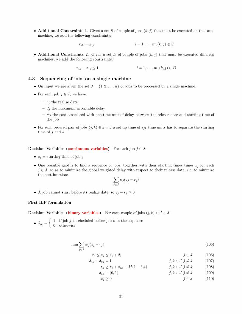
• 2-opt: given a heuristic TSP solution, choose two arcs, delete them and complete the circuit (only onepossible way).

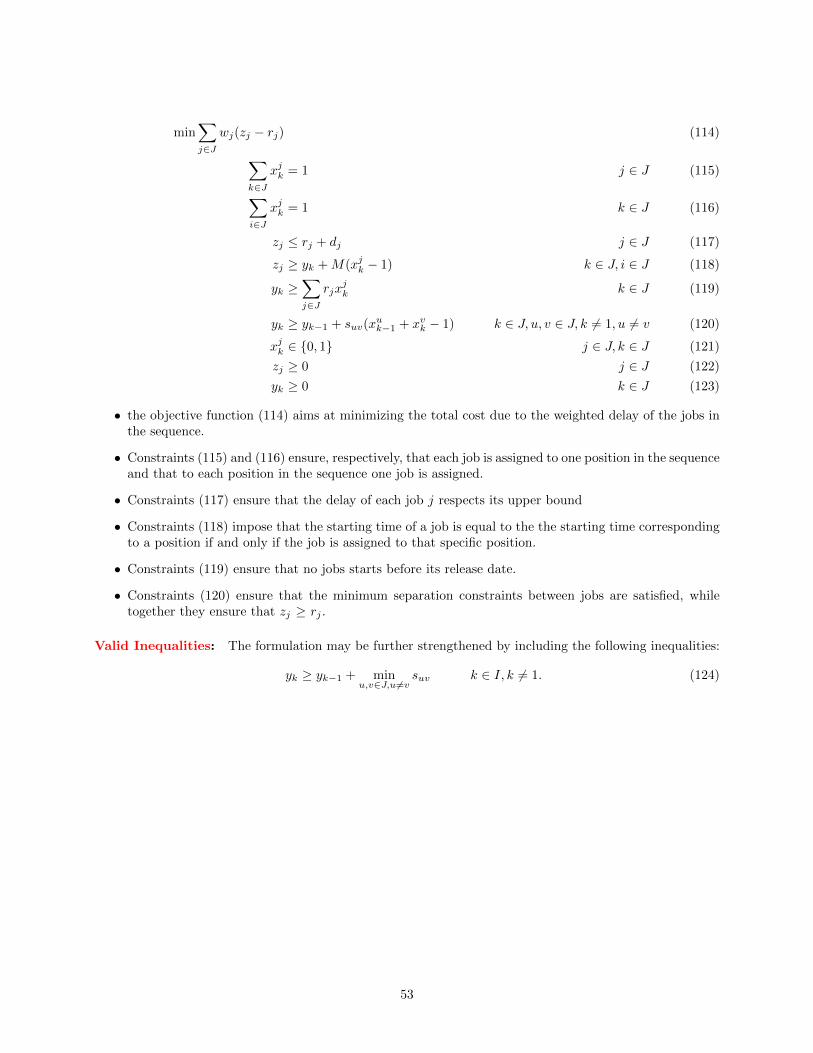
• 3-opt: given a heuristic TSP solution, choose three arcs, delete them and complete the circuit (differentpossible ways).

• Or-opt: given a heuristic TSP solution, choose a sequence of 3 vertices and try to insert it in all otherpossible positions. Then close the circuit (only one possible way).

Size of the neighborhoods for the TSP

• Swap: for each vertex (' n) consider all the other vertices (' n): n× n = O(n2) moves.

56

• 2-Opt: for each arc (' n) consider all the other arcs (' n): n× n = O(n2) moves.

• 3-Opt: for each arc (' n) consider all the other arcs (' n), and for each of them consider all the otherarcs (' n): n× n× n = O(n3) moves.

• For a graph of of 100 vertices (small) the complete exploration of the 3-Opt neighborhood requires' 1.000.000 attempts.

• The larger the neighborhood e the more effective is the local search but the computing time increasesaccordingly.

Multi start

• A search algorithm can be easily improved by applying it and different initial solutions.

• In addition Local Search algorithm can be applied recursively to the improved solutions found:

– first improvement: restart the local search on the first solution improved solution

– best improvement: completely explore the neighborhoods and restart the local search on the bestsolution found.

5.1 Genetic Algorithms

• The genetic algorithms (Holland 1975) are inspired by the evolution process of organisms in nature.

• These algorithms keep at each iteration a set of Solutions (or textitgenes), called population, which isupdated during the various iterations.

• The update consists of recombining different genes of the population, called parent set (typically pairsof individuals) to generate new solutions. The operation that, given a parent set, allows you to createa new gene is called crossover.

• In some cases a Repair Method is necessary to restore feasibility of a newly created gene

• A mutation is probabilistically performed on new genes of the population in order to diversify theprocess.

• The genes are coded as vectors. Typically two are the main encodings:

- Binary encoding 0/1

- Encoding as a permutation of values

Pseudocode

• Built an initial population P of initial genes P ;

• Evaluate the cost of each gene f(x),∀x ∈ P (f : fitness function);

• repeat

– Parent Selection: in function of the genes and their fitness, select a subset G of genes in P ;

– Crossover: built a set PG of genes combining the parents in G ;

– Mutation: random modification of a subset of genes of PG;

57

– Randomization: generate new genes;

– Let PG be the new set of genes;

– Perform a local search on each gene in PG

– Evaluate the fitness for the new gene in PG;

– Population selection: build a new population P by substituting all or some of the genes in P using

the set PG;

– Let P = P ;

• until <halting conditions>.

• Example: binary encoding of a gene

Single Crossover

(0 0 0 0 1 1 1)

(0 1 0 1 0 1 0)⇒

(0 0 0 0 0 1 0)

(0 1 0 1 1 1 1)

Double Crossover(0 0 0 0 1 1 1)

(0 1 0 1 0 1 0)⇒

(0 0 0 1 1 1 1)

(0 1 0 0 0 1 0)

Mutation(0 1 0 0 0 1 0)

↓(0 1 1 0 0 1 0)

58

Gestion de la production - lamsade.dauphine.frfurini/lib/exe/fetch.php?media=wiki:notes... ·...

Documents

Transcript of Gestion de la production - lamsade.dauphine.frfurini/lib/exe/fetch.php?media=wiki:notes... ·...