Geometer's Sketchpad Workshop - Salisbury...

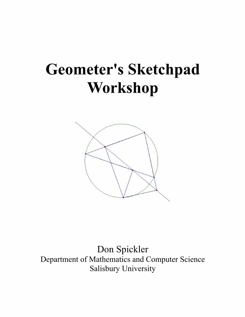
Geometer's Sketchpad Workshop

Don SpicklerDepartment of Mathematics and Computer Science

Salisbury University

Geometer's Sketchpad Workshop Outline 1. Basic Construction, Measurement and Transformation Features

(a) Program Layout and Free Play i. Toolbar Tools – Hold for other tool options. ii. Menus iii. Plotting and dragging points and lines. iv. Help System

(b) Basic Constructions and Hiding i. Construction of an equilateral triangle. ii. Construction of an isosceles triangle. iii. Construction of the isosceles triangle using the perpendicular bisector command. iv. Construction of an isosceles triangle, yet another way.

(c) Constructions i. Construct a square: The Geometer’s Sketchpad Workshop Guide: Tour 1:

Constructing a Square ii. Centers of Circles - Custom Tools - Extending GSP

A. Circumcenter and circumcircle. B. Median or Centriod. C. The Orthocenter. D. The Euler Line

iii. A Few More Examples A. Incenter and Incircle B. 9-Point Circle C. Simpson's Line D. Other Construction Options We Did Not Cover Above

(d) Measurements, Calculations and Captions i. Ratio of the Midpoint Segment of a Triangle. ii. Alternating Interior Angles iii. Internal Angles of a Triangle iv. The Geometer’s Sketchpad Workshop Guide: Tour 2: A Theorem About Quadrilaterals v. Pythagorean Theorem vi. Napoleon's Theorem vii. Other Measurement Exercises

A. Center verses Outside Angle of a Circle. B. Minimal Cost Experiment C. Opposite Angles of a Quadrilateral Inscribed Inside a Circle. D. Construction for Taking the Square Root of a Length. E. Ceva's Theorem F. The Fermat Point G. Radian Measure Exercise H. A Couple Measurements We Did not Do Above.

(e) Transformations i. Simple Translations, Reflections Rotations and Dilations.

A. Several Ways to Translate• Translating by a Fixed Amount:• Translating by a Distance:• Translating by a Vector:

B. Reflections C. Several Ways to Rotate

• Rotation by a Fixed Amount.• Rotation by an Angle.

D. Several Ways to Dilate• Dilation by a Fixed Amount.• Dilation by a Ratio.

ii. Name Writing Exercise. 2. Extending Beyond Basic Geometry

(a) Animation of Objects i. Add an animation to the Simpson line construction.

(b) Tracing i. Focus Directrix Construction of a Parabola using the Trace ii. Focus Directrix Construction of a Parabola using the Locus

(c) Action Buttons i. Show/Hide ii. Start/Stop Animations.

A. Spirograph Example iii. Multiple Documents and links to them.

(d) Slider Construction and Locking Objects to the Sketch. i. Sliders as Points on the x-axis ii. General Slider Construction

(e) Split/Merge option.(f) Tessellations:

i. Glide Example. ii. Rotation Example

(g) Constructions on Images Golden Ratio example. (h) Functions

i. Plotting Simple Functions. ii. Integrating Sliders with Functions iii. Derivatives and Tangent lines

(i) Iteration: Spiral Example(j) Tables: Circle Area verses Radius and an Approximation of π.(k) JavaSketchpad (JSP)

3. GeoGebra: Similarities and Differences with GSP.

Construction Examples

Construction of an Equilateral Triangle in GSP

Recall that an equilateral triangle is a triangle with all three of its sides equal in length. This is one of the first constructions we do since it is quick and so many more compensated constructions rely on it. In fact, it is the first proposition in the first book of Euclid's Elements (I.1). The way we would construct this with a straightedge and compass is to

1. Construct a generic line segment. 2. Construct a circle with center at one endpoint and radius the segment 3. Construct another circle with center at the other endpoint and radius the segment. 4. Connect one of the intersection points to each of the endpoints of the line segment.

With GSP you do the construction the same way.

1. Open up a new sketch. 2. Select the line segment tool and plot a line segment. 3. Select the circle tool. 4. Click on one endpoint and move the mouse to the other endpoint and click the other endpoint. 5. Now is a good time to do the “drag test”. Select the pointer/movement tool and click and drag

the endpoints of the segment. If the circle does not seem to be attached you need to back up and redo the construction. If it is attached go on to the next step. If you need to redo the circle construction simply click outside all of the objects, this will unselect everything. Now click on the circle and press the delete key. At this point the circle should disappear. You can now go back redo the first circle construction.

6. Select the circle tool. 7. Click on the other endpoint and move the mouse to the

first and click the endpoint. At this point you should have the image to the right.

8. Now select the point tool. 9. Move the mouse over one point of intersection, notice

the two circles will be highlighted, and click the mouse. 10. Click on the line segment tool. 11. Connect the point of intersections to the endpoints. At

this point we have our triangle. 12. Let's do another drag test. If you drag the vertices of the

triangle you will see that the triangle is always isosceles, 13. Clean-up: Click on the selection arrow tool and then right-

click on each circle and select Hide Circle from the context (popup) menu. Do not select the Delete option! When you delete an object it removes it from the sketch along with any construction that relies on it. When you are done you should see just the triangle.

14. Save your work to a file by selecting File > Save from the main menu. Call the file something like EquilateralTriangle.gsp. Note that the program will put the “.gsp” extension on automatically.

Construction of an Isosceles Triangle in GSP

Recall that an isosceles triangle is a triangle with two of its sides equal in length. The way we would construct this with a straightedge and compass is to

1. Construct a generic line segment. 2. Construct a perpendicular bisector to that segment.

(a) Construct a circle with center at one endpoint and radius the segment (b) Construct another circle with center at the other endpoint and radius the segment.(c) The line connecting the intersections of the two circles is the perpendicular bisector.

3. Plot a point on that bisector 4. Connect the new point to the two endpoints of the original line segment.

With GSP you do the construction the same way. There are some shortcuts that can be made, which we will look at later, but for now we will do it the same way we would with a straightedge and compass.

1. Open up a new sketch. 2. Select the line segment tool and plot a line segment. 3. Select the circle tool. 4. Click on one endpoint and move the mouse to the other endpoint and click the other endpoint. 5. Now is a good time to do the “drag test”. Select the pointer/movement tool and click and drag

the endpoints of the segment. If the circle does not seem to be attached you need to back up and redo the construction. If it is attached go on to the next step. If you need to redo the circle construction simply click outside all of the objects, this will unselect everything. Now click on the circle and press the delete key. At this point the circle should disappear. You can now go back redo the first circle construction.

6. Select the circle tool. 7. Click on the other endpoint and move the mouse to the

first and click the endpoint. At this point you should have the image to the right.

8. Now select the point tool. We need to put points on the intersections so that we can plot a line between them.

9. Move the mouse over one point of intersection, notice the two circles will be highlighted, and click the mouse.

10. Do the same for the other point of intersection. 11. Do a drag test. 12. Select the line tool, remember you need to click and hold the line button to get the sub-toolbar

and then select the infinite line. 13. Click on one point of intersection and then click on the

other. This should produce the perpendicular bisector to the segment.

14. Click on the point tool. 15. Click on the perpendicular bisector. This will lock the

point to the perpendicular bisector. 16. Click on the line segment tool. 17. Connect the point on the perpendicular bisector to one

of the endpoints. Then do the same to the other endpoint. At this point we have our triangle.

18. Let's do another drag test. If you drag the vertices of the triangle you will see that the triangle is always isosceles,

19. Clean-up: Click on the selection arrow tool and then right-click on each circle and select Hide Circle from the context (popup) menu. Do not select the Delete option! When you delete an object it removes it from the sketch along with any construction that relies on it. Do the same for the perpendicular bisector and the intersection points. When you are done you should see just the triangle.

20. Save your work to a file by selecting File > Save from the main menu. Call the file something like IsoscelesTriangle.gsp. Note that the program will put the “.gsp” extension on automatically.

Construction of an Isosceles Triangle in GSP (a little quicker)

The above method is good pedagogically since it uses only the straightedge and compass tools. From a mathematical standpoint this verifies that the ability to construct an isosceles triangle and a perpendicular bisector follows from the axioms of Euclidean geometry. Once the student knows that the perpendicular bisector can be constructed and how to do it they can use the construction menu in GSP to take a shortcut. Here is how we would proceed with creating the isosceles triangle.

1. Open up a new sketch. 2. Select the line segment tool and plot a line segment. 3. Click somewhere outside the object to unselect everything. 4. Click on the line segment (but not the endpoints) 5. Select Construct > Midpoint from the menu. At this point the midpoint to the segment will

appear. 6. Click on the line segment again, so that both the line segment and the midpoint are selected. 7. Select Construct > Perpendicular Line from the menu. At this point a line perpendicular to the

segment and passing through the midpoint will appear. 8. Click on the point tool. 9. Click on the perpendicular bisector. This will lock the point to the perpendicular bisector. 10. Click on the line segment tool. 11. Connect the point on the perpendicular bisector to

one of the endpoints. Then do the same to the other endpoint. At this point we have our triangle.

12. Let's do a drag test. 13. Clean-up: Click on the selection arrow tool and

then right-click on the perpendicular bisector and select the hide option. Do the same with the midpoint.

14. Save your work to a file by selecting File > Save from the main menu. Call the file something like IsoscelesTriangle2.gsp. Note that the program will put the “.gsp” extension on automatically.

Construction of an Isosceles Triangle in GSP (YAW – Yet Another Way)

Another way to construct an isosceles triangle is to simply construct a circle put two radii on it and connect the cord of the radii.

1. Open up a new sketch. 2. Select the circle tool and plot a circle. Notice that there is a

point at the center and a point on the circle itself. 3. Select the line segment tool. 4. Plot a line segment from the center of the circle to the point on

the circle. 5. Plot another line segment from the center of the circle to the

circle. Here you will start at the center and when you get close to the circle itself it will be highlighted, simply click on the circle when it is highlighted and GSP will place a new point there.

6. Now connect the two points on the circle with a line segment. 7. Do a drag test. 8. Clean it up by hiding the circle and make sure you save your work.

Personally, I like the other methods for constructing an isosceles triangle. Even though they are a little more complicated the way the triangle acts under the drag test seems more natural.

Centers of Triangles and The Euler Line

Now that we have got some practice with constructions in GSP let's look at something a bit longer. There are several types of centers to a given triangle. In this exercise we will construct three of them: the circumcenter, the median (or centroid), orthocenter. We will also use these constructions to create new tools for the toolbar and then find an interesting relationship between them.

The Circumcenter

As its name implies, the circumcenter is the center of the circumcircle, which is the center of the unique circle that passes through the vertices of the triangle. The circumcenter is the point of intersection of the perpendicular bisectors to the sides of the triangle. Doing all of the constructions using the straightedge and compass tools would be lengthy and create a messy construction. Since we know that these can all be done with the straightedge and compass we will use the shortcut construction tools from the menu..

1. Open a new sketch.2. Create a triangle with the Line Segment tool.3. Select all of the sides of the triangle and select Construct > Midpoints from the menu.4. Click outside the construction to unselect everything.5. Select one segment and its midpoint. Select Construct > Perpendicular Line from the menu.6. Do the same for the other two sides.7. Do a drag test. Notice that the three perpendicular lines always intersect at the same point.

This is the circumcenter of the triangle.8. Select the point tool and click on the point of intersection of the three lines. Before you click,

notice that as you hover the mouse over the intersection point you can only get two of the three lines to highlight at the same time. This is because GSP will only find the intersection between two lines at one time.

9. (Optional) There is another way to construct an intersection point (or points) between two objects. Sometimes it is difficult to move the mouse over two objects at the same time and even if you do get the mouse in the correct position when you click the button it is very easy to move the mouse off the intersection point at the same time. So instead you can select the two objects and then select Construct > Intersection from the menu.

10. Now that we have the circumcenter lets construct the circumcircle. Select the circle tool and create a circle with center at the intersection point (the circumcenter) and place the other point on any one of the vertices.

11. Do a drag test. Note that the circle always goes through the three vertices.

12. Now we are going to create a custom tool for finding the circumcenter. When you create a custom tool you must select the objects that create the thing of interest, in this case the three vertices to the triangle, and the thing that is the result you want. We could simply select everything by then all we want is the circumcenter, we don't want to see the circle, perpendicular lines, midpoints and even the sides of the triangle. Select the selection pointer from the toolbar, click outside the construction to unselect everything, and select the three vertices of the triangle along with the circumcenter point.

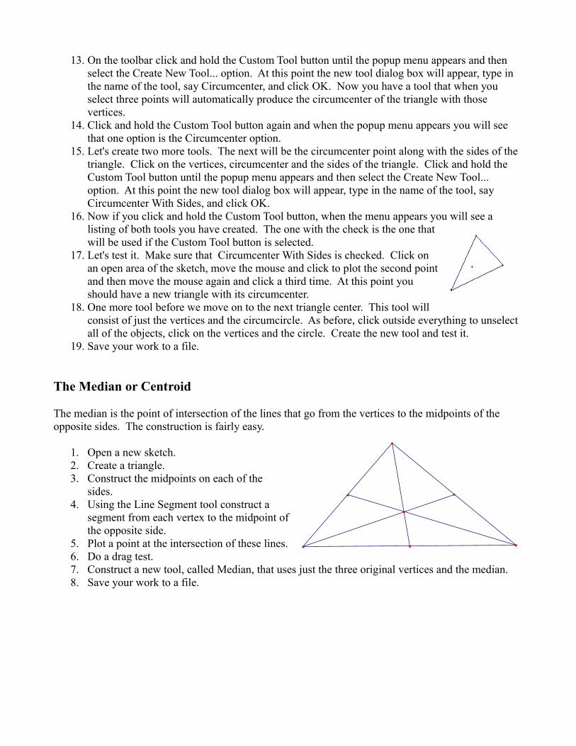
13. On the toolbar click and hold the Custom Tool button until the popup menu appears and then select the Create New Tool... option. At this point the new tool dialog box will appear, type in the name of the tool, say Circumcenter, and click OK. Now you have a tool that when you select three points will automatically produce the circumcenter of the triangle with those vertices.

14. Click and hold the Custom Tool button again and when the popup menu appears you will see that one option is the Circumcenter option.

15. Let's create two more tools. The next will be the circumcenter point along with the sides of the triangle. Click on the vertices, circumcenter and the sides of the triangle. Click and hold the Custom Tool button until the popup menu appears and then select the Create New Tool... option. At this point the new tool dialog box will appear, type in the name of the tool, say Circumcenter With Sides, and click OK.

16. Now if you click and hold the Custom Tool button, when the menu appears you will see a listing of both tools you have created. The one with the check is the one that will be used if the Custom Tool button is selected.

17. Let's test it. Make sure that Circumcenter With Sides is checked. Click on an open area of the sketch, move the mouse and click to plot the second point and then move the mouse again and click a third time. At this point you should have a new triangle with its circumcenter.

18. One more tool before we move on to the next triangle center. This tool will consist of just the vertices and the circumcircle. As before, click outside everything to unselect all of the objects, click on the vertices and the circle. Create the new tool and test it.

19. Save your work to a file.

The Median or Centroid

The median is the point of intersection of the lines that go from the vertices to the midpoints of the opposite sides. The construction is fairly easy.

1. Open a new sketch. 2. Create a triangle.3. Construct the midpoints on each of the

sides.4. Using the Line Segment tool construct a

segment from each vertex to the midpoint of the opposite side.

5. Plot a point at the intersection of these lines.6. Do a drag test.7. Construct a new tool, called Median, that uses just the three original vertices and the median.8. Save your work to a file.

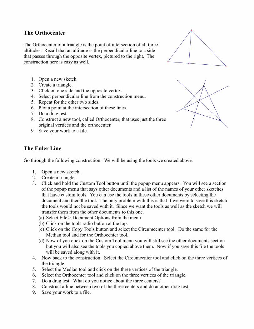
The Orthocenter

The Orthocenter of a triangle is the point of intersection of all three altitudes. Recall that an altitude is the perpendicular line to a side that passes through the opposite vertex, pictured to the right. The construction here is easy as well.

1. Open a new sketch. 2. Create a triangle.3. Click on one side and the opposite vertex. 4. Select perpendicular line from the construction menu. 5. Repeat for the other two sides. 6. Plot a point at the intersection of these lines.7. Do a drag test.8. Construct a new tool, called Orthocenter, that uses just the three

original vertices and the orthocenter.9. Save your work to a file.

The Euler Line

Go through the following construction. We will be using the tools we created above.

1. Open a new sketch. 2. Create a triangle. 3. Click and hold the Custom Tool button until the popup menu appears. You will see a section

of the popup menu that says other documents and a list of the names of your other sketches that have custom tools. You can use the tools in these other documents by selecting the document and then the tool. The only problem with this is that if we were to save this sketch the tools would not be saved with it. Since we want the tools as well as the sketch we will transfer them from the other documents to this one.

(a) Select File > Document Options from the menu. (b) Click on the tools radio button at the top.(c) Click on the Copy Tools button and select the Circumcenter tool. Do the same for the

Median tool and for the Orthocenter tool. (d) Now of you click on the Custom Tool menu you will still see the other documents section

but you will also see the tools you copied above them. Now if you save this file the tools will be saved along with it.

4. Now back to the construction. Select the Circumcenter tool and click on the three vertices of the triangle.

5. Select the Median tool and click on the three vertices of the triangle. 6. Select the Orthocenter tool and click on the three vertices of the triangle. 7. Do a drag test. What do you notice about the three centers? 8. Construct a line between two of the three centers and do another drag test. 9. Save your work to a file.

A Few More Construction Examples

The Incenter and Incircle

The incircle is the unique circle that is inscribed inside a triangle. The center of this circle is at the intersection point of the three angle bisectors of the triangle. So to construct the incircle we need to first construct the incenter and then drop a perpendicular from the incenter to a side, this gives the radius and then finally construct a circle with center at the incenter and radius out to the point of intersection between the side and perpendicular.

1. Open a new sketch. 2. Create a triangle. 3. GSP also has the ability to label any of its

objects. To turn on a label simply right-click on an object and select to turn on the labeling. Do so for the three vertices. You can change the label by right clicking on the object and selecting properties. You can also change the font of the label. The properties dialog has other information in it, such as the parents and children of the object.

4. At this point we are going to construct the angle bisectors. As before we could go through the straightedge and compass construction of them but there is a construction option for these as well. When constructing an angle bisector you first need to select the angle by clicking on the vertices in order.

5. Select the vertices A, B, and C in that order. Then select Construct > Angle Bisector. 6. Select the vertices B, C, and A in that order. Then select Construct > Angle Bisector. 7. Select the vertices C, A, and B in that order. Then select Construct > Angle Bisector. 8. Plot the intersection point. This gives us the incenter. 9. Plot the perpendicular to one side passing through the incenter. 10. Plot the point of intersection between the side and perpendicular. 11. Finally construct the circle with center of the incenter and edge at the intersection point. 12. Do a drag test and save your work.

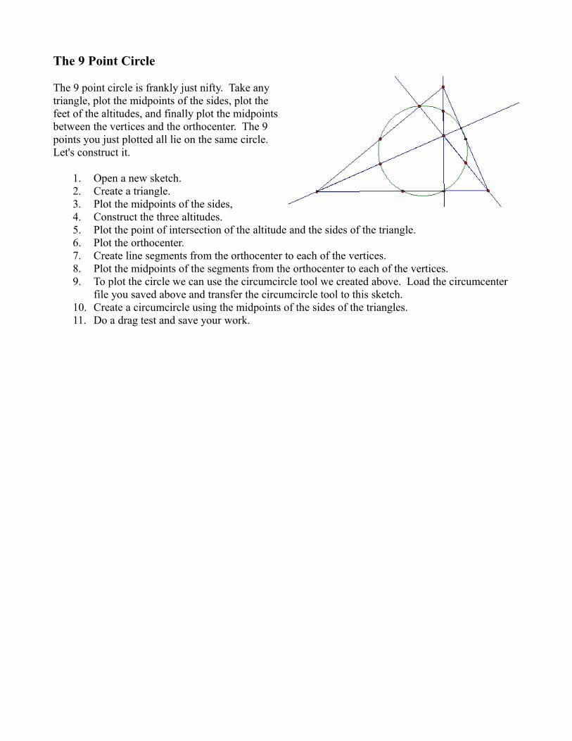
The 9 Point Circle

The 9 point circle is frankly just nifty. Take any triangle, plot the midpoints of the sides, plot the feet of the altitudes, and finally plot the midpoints between the vertices and the orthocenter. The 9 points you just plotted all lie on the same circle. Let's construct it.

1. Open a new sketch. 2. Create a triangle. 3. Plot the midpoints of the sides, 4. Construct the three altitudes. 5. Plot the point of intersection of the altitude and the sides of the triangle. 6. Plot the orthocenter. 7. Create line segments from the orthocenter to each of the vertices. 8. Plot the midpoints of the segments from the orthocenter to each of the vertices. 9. To plot the circle we can use the circumcircle tool we created above. Load the circumcenter

file you saved above and transfer the circumcircle tool to this sketch. 10. Create a circumcircle using the midpoints of the sides of the triangles. 11. Do a drag test and save your work.

The Simpson Line

The Simpson Line is another nifty relationship between a triangle and a circle. Take a triangle and construct its circumcircle. Place a point on the circumcircle and drop a perpendicular line from that point to the three sides of the triangle. If you look at the three points of intersection you will see that they lie on a straight line. Although this construction is similar to the ones we did above it does show a situation where the initial triangle construction and the cleanup stage takes a little more care so that the reader can better visualize the construction.

1. Open a new sketch. 2. Create a triangle using the infinite line tool. We will see

later why we are using the infinite line tool instead of the line segment tool. 3. Load in the circumcircle example we did above and transfer the circumcircle tool to this

sketch. Use it to construct the circumcircle to this triangle. 4. Plot a point on the circle. 5. Now we will construct the perpendicular lines. GSP allows to do several constructions at the

same time as long as you set them up correctly. Here we will construct all three perpendicular lines at the same time. Select just the point on the circle and the three sides of the triangle. Select Construct > Perpendicular Lines from the menu and all three perpendiculars should appear.

6. Plot the points of intersection between each perpendicular and its respective side. 7. Construct an infinite line between two of the three points of intersection you plotted above. 8. Do a drag test. Can you see why we chose to use the infinite lines in place of the line

segments for this construction? 9. Time to clean up the construction.

(a) First, all of the infinite lines in the sketch are distracting. Hide all of the infinite lines except for the Simpson Line.

(b) Now this will remove the original triangle, which we want, so put line segments in for the sides of the triangle.

(c) We also want to see the perpendicular lines but it is sufficient for them to stop at the triangle, so put in line segments for these.

(d) Do a drag test. Does anything happen that might be a little strange for the person using this sketch?

(e) Construct a line segment from each point of intersection (the ones on the Simpson Line) to one of the endpoints of the side of the triangle that the point lies.

(f) Do another drag test and save your work.

Other Construction Options We Did Not Cover Above

In this exercise we will simply look at at some other construction options.

Circle By Center+Point

1. Open a new sketch. 2. Plot two points. 3. Select the two points. 4. Select Construct > Circle By Center+Point. This will create a circle in much the same way as

the compass tool. 5. Do a drag test.

Circle By Center+Radius

1. Open a new sketch. 2. Plot a line segment and a point not on that segment. 3. Select Construct > Circle By Center+Radius. 4. Do a drag test. Notice what happens when you change the length of the line segment.

Arc On Circle

1. Open a new sketch. 2. Construct a circle. 3. Plot two points on the circle and label them A and B. 4. Plot segments from the points and center of the circle. 5. Select the two points on the circle in a counter clockwise order and

select the circle itself. 6. Select Construct > Arc On Circle. This creates an arc from A to B. 7. Hide the original circle and you should have the sector pictured to the

right.

Arc Through 3 Points

1. Open a new sketch. 2. Plot three points. 3. Select the three points. 4. Select Construct > Arc Through 3 Points. Notice that it almost does

what our circumcircle tool does.

BA

Locus

A locus of points is the set of points that a driven object maps out as a driver object moves along a path. As an easy example consider the diagram to the right. It is simply a circle with one point on the circle and one point off the circle. We then construct the segment between these two and construct the midpoint of the segment. Now the point on the circle is the driver object and the midpoint is the driven object. As the point on the circle moves around the circle the midpoint will map out a smaller circle to the right. This smaller circle is the locus of points created by the smaller circle. Here is one way to graph this with GSP.

1. Open a new sketch. 2. Construct a circle. 3. Plot a point on the circle and a point off to the

right of the circle. 4. Construct the line segment between them. 5. Plot the midpoint to the segment. 6. Select the point on the circle and the midpoint. 7. Select Construct < Locus from the menu. You

should see the image to the right. 8. Do a drag test. Notice what happens when you drag the point on the circle around the circle.

Measurement Examples

Ratio of the Midpoint Segment of a Triangle.

This example is a very simple one that uses some basic measurement and calculation facilities of GSP. The goal is to find the ratio of the lengths of a side of a triangle and the segment joining the midpoints of the other two sides. The result is, of course, 0.5 but it will get us acclimated to GSP measurements.

1. Open a new sketch. 2. Create a triangle. 3. Plot the midpoints of two of the sides. 4. Join the midpoints with a line segment. 5. Select the segment you just drew along with the side of the triangle that is parallel to it. 6. Select Measure > Length from the menu. Notice that several things

happened. First, GSP labeled all of the points that it needed in the length calculations. Second the lengths are not in the upper left corner of the sketch. Calculation boxes can be selected and moved just like a free point.

7. Do a drag test. Notice that values of the lengths change as you move the vertices of the original triangle.

8. Now we could simply notice that the side length was always twice that of the midpoint segment but we will go one step further with the example.

9. Select Measure > Calculate from the menu. At this point the calculator dialog box will appear.

10. We wish to take a ratio of the two lengths. Click on the length calculation of the midpoint segment. Notice that it was transferred to the calculator. Also notice that some of the keys of the calculator changed from enabled to disabled and disabled to enabled. The GSP calculator is set up so that making a syntax error in your calculation is not possible. Click the division symbol and then the other length measurement. Click the OK button. The calculation should now be in the sketch.

11. Do another drag test and save your work.

m AB

m CD = 0.50

m CD = 6.50 cm

m AB = 3.25 cm

BA

DC

Alternating Interior Angles

Alternating interior angles between two parallel lines are equal. Here is a quick measurement exercise to verify this.

1. Open a new sketch. 2. Draw an infinite line. 3. Plot a point not on that line and label it A. 4. Construct a line through A parallel to the first line. 5. Plot a point on the original line and one on the

constructed parallel line. Label the point on the parallel line as B and the one on the original line as C.

6. Label the far right point on the original line as D. 7. To measure an angle in GSP you need to select the three points that make the angle. Click

outside the construction to make sure that nothing is selected. Now click on the points A, B and C in that order. Now select Measure > Angle from the menu and you should see the angle measurement in the upper left. Do the same with the other angle, make sure that you select B, C and D in that order.

8. Do a drag test and save your work.

Internal Angles of a Triangle

This example is to simply verify that the sum of the interior angles of a triangle is 180 degrees.

1. Open a new sketch. 2. Create a triangle. 3. Measure each of the interior angles of the triangle. 4. Calculate the sum of the three angles. 5. Do a drag test and save your work.

m ∠ CAB = 62.86 °

m ∠ BCA = 44.11 °

m ∠ ABC = 73.03 °

B

CA

The Pythagorean Theorem

This clearly needs no introduction. We will do the famed windmill construction. As we all know this theorem is usually remembered as a2 + b2 = c2, which seems to be a relationship with lengths. Although the original intent of the Pythagoreans was to establish a relationship with areas. We will take the Pythagorean point of view here. We will need to first construct a right triangle and then place squares on each of the sides. This could be a lot of constructions but we will take a shortcut. In Tour 1: Creating the Square we went through the construction of the square. In that example we did not create a new tool from the construction but we will do so now.

1. Open up the file that had the Creating the Square example. 2. Create a new tool, called Square, from the construction. 3. Open a new sketch for the Pythagorean Theorem construction. 4. Copy the Square Tool to the new sketch.

The Pythagorean Theorem Construction

1. The first step is to construct a generic right triangle. As usual this is done as you would on paper with the usual GSP shortcuts. (a) Construct a line segment. (b) Construct a perpendicular line to the segment passing through one of the endpoints. (c) Plot a point on the perpendicular line.(d) Draw a segment from the point on the perpendicular to the other endpoint of the line

segment.(e) Hide the perpendicular line and construct a line segment to finish out the right triangle.(f) Do a drag test.

2. Now we are ready to construct the squares. Select the Square tool you constructed and place squares on the sides of the triangle by selecting the two endpoints for the side. One thing you will notice is that the square might be outside the triangle or inside the triangle. This all depends on the order in which you select the endpoints. If the square is going the wrong way step back (with Ctrl+Z) and select the endpoints in a different order.

3. Now we need to create areas. Click on the vertices of one of the squares and select Construct > Quadrilateral Area. Do the same for the other two squares.

4. When you construct the areas the regions will all be yellow. Change the colors so that each square is a different color.

5. To get the measurements of the areas select an area and then select Measure > Area from the menu. Do this for all of the squares and change the colors of the measurements to correspond with the colors of the squares they measure.

6. Finally calculate the sum of the two smaller squares. 7. Do a drag test and save your work.

Area BEFG( ) + Area CGHI( ) = 12.35 cm 2

Area CGHI = 8.66 cm 2

Area BEFG = 3.69 cm 2

Area ABCD = 12.35 cm 2

I H

F

E

A

D

C G

B

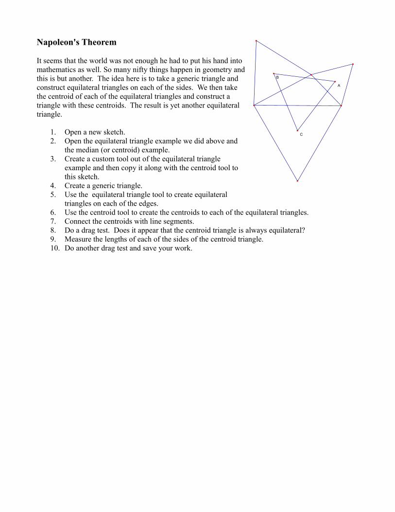
Napoleon's Theorem

It seems that the world was not enough he had to put his hand into mathematics as well. So many nifty things happen in geometry and this is but another. The idea here is to take a generic triangle and construct equilateral triangles on each of the sides. We then take the centroid of each of the equilateral triangles and construct a triangle with these centroids. The result is yet another equilateral triangle.

1. Open a new sketch. 2. Open the equilateral triangle example we did above and

the median (or centroid) example. 3. Create a custom tool out of the equilateral triangle

example and then copy it along with the centroid tool to this sketch.

4. Create a generic triangle. 5. Use the equilateral triangle tool to create equilateral

triangles on each of the edges. 6. Use the centroid tool to create the centroids to each of the equilateral triangles. 7. Connect the centroids with line segments. 8. Do a drag test. Does it appear that the centroid triangle is always equilateral? 9. Measure the lengths of each of the sides of the centroid triangle. 10. Do another drag test and save your work.

C

A

B

Other Measurement Exercises

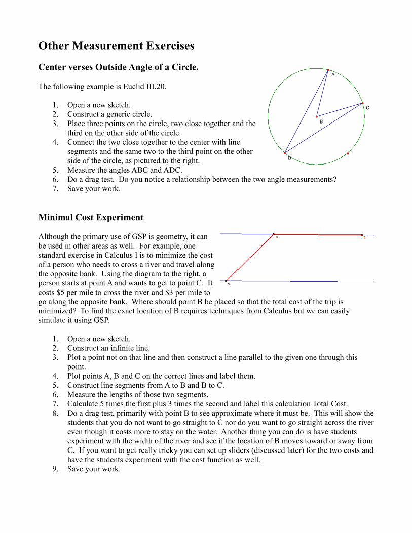
Center verses Outside Angle of a Circle.

The following example is Euclid III.20.

1. Open a new sketch. 2. Construct a generic circle. 3. Place three points on the circle, two close together and the

third on the other side of the circle. 4. Connect the two close together to the center with line

segments and the same two to the third point on the other side of the circle, as pictured to the right.

5. Measure the angles ABC and ADC. 6. Do a drag test. Do you notice a relationship between the two angle measurements? 7. Save your work.

Minimal Cost Experiment

Although the primary use of GSP is geometry, it can be used in other areas as well. For example, one standard exercise in Calculus I is to minimize the cost of a person who needs to cross a river and travel along the opposite bank. Using the diagram to the right, a person starts at point A and wants to get to point C. It costs $5 per mile to cross the river and $3 per mile to go along the opposite bank. Where should point B be placed so that the total cost of the trip is minimized? To find the exact location of B requires techniques from Calculus but we can easily simulate it using GSP.

1. Open a new sketch. 2. Construct an infinite line. 3. Plot a point not on that line and then construct a line parallel to the given one through this

point. 4. Plot points A, B and C on the correct lines and label them. 5. Construct line segments from A to B and B to C. 6. Measure the lengths of those two segments. 7. Calculate 5 times the first plus 3 times the second and label this calculation Total Cost. 8. Do a drag test, primarily with point B to see approximate where it must be. This will show the

students that you do not want to go straight to C nor do you want to go straight across the river even though it costs more to stay on the water. Another thing you can do is have students experiment with the width of the river and see if the location of B moves toward or away from C. If you want to get really tricky you can set up sliders (discussed later) for the two costs and have the students experiment with the cost function as well.

9. Save your work.

B

A

C

D

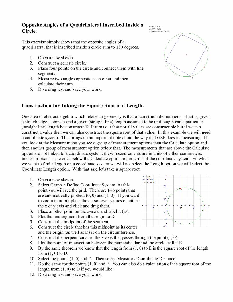
Opposite Angles of a Quadrilateral Inscribed Inside a Circle.

This exercise simply shows that the opposite angles of a quadrilateral that is inscribed inside a circle sum to 180 degrees.

1. Open a new sketch. 2. Construct a generic circle. 3. Place four points on the circle and connect them with line

segments. 4. Measure two angles opposite each other and then

calculate their sum. 5. Do a drag test and save your work.

Construction for Taking the Square Root of a Length.

One area of abstract algebra which relates to geometry is that of constructible numbers. That is, given a straightedge, compass and a given (straight line) length assumed to be unit length can a particular (straight line) length be constructed? It turns out that not all values are constructible but if we can construct a value then we can also construct the square root of that value. In this example we will need a coordinate system. This brings up an important note about the way that GSP does its measuring. If you look at the Measure menu you see a group of measurement options then the Calculate option and then another group of measurement option below that. The measurements that are above the Calculate option are not linked to a coordinate system, these measurements are in units of either centimeters, inches or pixels. The ones below the Calculate option are in terms of the coordinate system. So when we want to find a length on a coordinate system we will not select the Length option we will select the Coordinate Length option. With that said let's take a square root.

1. Open a new sketch. 2. Select Graph > Define Coordinate System. At this

point you will see the grid. There are two points that are automatically plotted, (0, 0) and (1, 0). If you want to zoom in or out place the cursor over values on either the x or y axis and click and drag them.

3. Place another point on the x-axis, and label it (D). 4. Plot the line segment from the origin to D. 5. Construct the midpoint of the segment. 6. Construct the circle that has this midpoint as its center

and the origin (as well as D) is on the circumference. 7. Construct the perpendicular to the x-axis that passes through the point (1, 0). 8. Plot the point of intersection between the perpendicular and the circle, call it E. 9. By the same theorem we know that the length from (1, 0) to E is the square root of the length

from (1, 0) to D. 10. Select the points (1, 0) and D. Then select Measure > Coordinate Distance. 11. Do the same for the points (1, 0) and E. You can also do a calculation of the square root of the

length from (1, 0) to D if you would like. 12. Do a drag test and save your work.

m ∠ BAD+m ∠ BCD = 180.00°

m ∠ BCD = 88.89°

m ∠ BAD = 91.11°

B

C

D

A

Ceva's Theorem

Ceva's Theorem is a theorem on the relationships of ratios of lengths in a generic triangle. Given any triangle and any point in the interior of the triangle if you construct lines through each vertex and the interior point and take the intersection of that line with the side of the triangle, as pictured to the right, you wind up with the following relation.

1. Open a new sketch. 2. Create a triangle. 3. Plot a point inside the triangle. 4. Select either the ray tool or the infinite line tool. 5. Plot lines from each vertex to the interior point. 6. Plot the intersection points of these lines and the sides of the triangle. 7. Hide the lines or rays and replace each with a line segment as shown in the sketch above. 8. Turn the labels on for all of the points, remember the quick way to do this is to select all of the

pints at one time and then select Display > Show Labels from the menu. 9. Select the points A and F and then select Measure > Distance from the menu. 10. Do the same for the other 5 lengths. 11. Create the calculation above. 12. Do a drag test and save your work.

F

DG

A

B

C

E

FA

FC( ) ⋅DC

BD( ) ⋅GB

AG( ) = 1.00

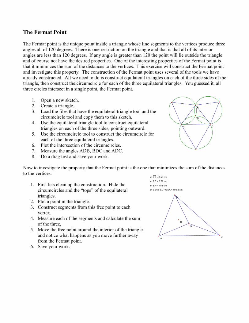
The Fermat Point

The Fermat point is the unique point inside a triangle whose line segments to the vertices produce three angles all of 120 degrees. There is one restriction on the triangle and that is that all of its interior angles are less than 120 degrees. If any angle is greater than 120 the point will lie outside the triangle and of course not have the desired properties. One of the interesting properties of the Fermat point is that it minimizes the sum of the distances to the vertices. This exercise will construct the Fermat point and investigate this property. The construction of the Fermat point uses several of the tools we have already constructed. All we need to do is construct equilateral triangles on each of the three sides of the triangle, then construct the circumcircle for each of the three equilateral triangles. You guessed it, all three circles intersect in a single point, the Fermat point.

1. Open a new sketch. 2. Create a triangle. 3. Load the files that have the equilateral triangle tool and the

circumcircle tool and copy them to this sketch. 4. Use the equilateral triangle tool to construct equilateral

triangles on each of the three sides, pointing outward. 5. Use the circumcircle tool to construct the circumcircle for

each of the three equilateral triangles. 6. Plot the intersection of the circumcircles. 7. Measure the angles ADB, BDC and ADC. 8. Do a drag test and save your work.

Now to investigate the property that the Fermat point is the one that minimizes the sum of the distances to the vertices.

1. First lets clean up the construction. Hide the circumcircles and the “tops” of the equilateral triangles.

2. Plot a point in the triangle.3. Construct segments from this free point to each

vertex.4. Measure each of the segments and calculate the sum

of the three,5. Move the free point around the interior of the triangle

and notice what happens as you move further away from the Fermat point.

6. Save your work.

D

A

B

C

m EB+m EC+m EA = 10.68 cm

m EA = 3.58 cm

m EC = 3.60 cm

m EB = 3.50 cm

D

A

B

C

E

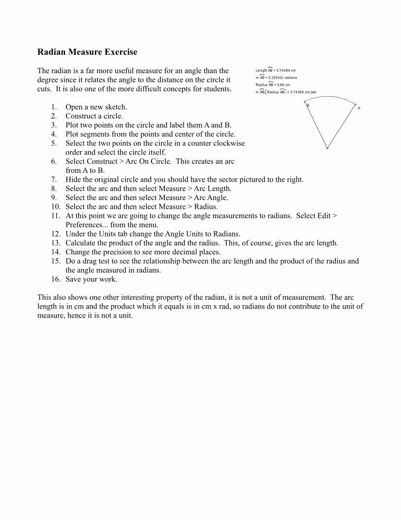
Radian Measure Exercise

The radian is a far more useful measure for an angle than the degree since it relates the angle to the distance on the circle it cuts. It is also one of the more difficult concepts for students.

1. Open a new sketch. 2. Construct a circle. 3. Plot two points on the circle and label them A and B. 4. Plot segments from the points and center of the circle. 5. Select the two points on the circle in a counter clockwise

order and select the circle itself. 6. Select Construct > Arc On Circle. This creates an arc

from A to B. 7. Hide the original circle and you should have the sector pictured to the right. 8. Select the arc and then select Measure > Arc Length. 9. Select the arc and then select Measure > Arc Angle. 10. Select the arc and then select Measure > Radius. 11. At this point we are going to change the angle measurements to radians. Select Edit >

Preferences... from the menu. 12. Under the Units tab change the Angle Units to Radians. 13. Calculate the product of the angle and the radius. This, of course, gives the arc length. 14. Change the precision to see more decimal places. 15. Do a drag test to see the relationship between the arc length and the product of the radius and

the angle measured in radians. 16. Save your work.

This also shows one other interesting property of the radian, it is not a unit of measurement. The arc length is in cm and the product which it equals is in cm x rad, so radians do not contribute to the unit of measure, hence it is not a unit.

m AB⋅ Radius AB( ) = 3.74384 cm ⋅ rad

Radius AB = 3.66 cm

m AB = 0.32542π radians

Length AB = 3.74384 cm

BA

A Couple Measurements We Did not Do Above.

We did most of the possible measurements the GSP can do above but there are two others in the coordinate system area Slope and Equation that we did not discuss. Now the names imply that they will measure the slope of a line and display the equation of a line or curve, which is precisely what they do but you need to be careful with the equation option when you alter the coordinate system.

Slope

1. Open a new sketch. 2. Construct a line, ray or line segment. 3. Select the line. 4. Select Measure > Slope from the menu and you will see the slope in the upper left of the

sketch. Notice that the grid is automatically shown when you do this. That is because GSP needs the grid to do the calculation. You could have selected to define the coordinate system first but it was not necessary.

5. Do a drag test. Note how the slope changes.

Equation

1. Open a new sketch. 2. Construct a line, ray or line segment. 3. Construct a circle. 4. Select the line. 5. Select Measure > Equation from the menu. Again the coordinate system will appear. 6. Select the circle. 7. Select Measure > Equation from the menu. 8. Do a drag test. Note how the equations change as you drag the objects.

Now lets see how this could lead to confusion. If you did not alter the grid at all it is probably in rectangular coordinates with the scale in the x direction the same as the scale in the y direction, in other words a square grid. Just to make sure select Graph > Grid Form from the menu and see if Square grid is checked. If not, Select it. Now go back to the sketch, place the mouse over a number, notice the pointer change then click and drag the number and notice what happens. Now go back to the Graph > Grid Form menu and select Rectangular Grid. Now click on a number on the x-axis and drag it. Notice that the y-axis is not locked to the x-axis anymore and more importantly look at the equation of the circle. Notice that the fractions on the left are divided by different values this means that the “circle” equation is now of the form a(x-h)2+b(y-k)2 = s where a and b are different. That is, this is now the equation of an ellipse. On the one hand this is fine, circle plotted on different axes scales is an ellipse but on the other hand your students are looking at a circle on the screen that is not really a circle.

Transformation Exercises

Simple Translations, Reflections Rotations and Dilations.

This example is simply to show you how to set up and use the Transformation menu options. We will look at all of the options in this menu except for Iterate, which we will deal with in the Advanced portion of this workshop.

Several Ways to Translate

Translating by a Fixed Amount:

1. Open a new sketch. 2. Construct a circle. 3. Select the circle. 4. Select Transform > Translate... from the menu. At this

point a translation dialog box will appear, pictured to the right. At the top is the transformation type. The options are a polar vector, a rectangular vector and marked, which is grayed out at this point and will be discussed below. The polar option will allow you to select a distance and angle for translation and the rectangular option will allow you select a horizontal and vertical shift.

5. Make sure that Rectangular is selected and lets make the horizontal distance 1 cm and the vertical distance 2 cm.

6. Click Translate. At this point you will see your original circle and the translation by (1, 2).


Translating by a Distance:

1. Open a new sketch. 2. Construct a circle. 3. Construct a line segment. 4. Select the line segment and measure its length. 5. Select the length calculation and then select Transform

> Mark Distance. 6. Select the circle. 7. Select Transform > Translate... from the menu. At this

point a translation dialog box will appear, pictured to the right. Since we marked a distance we now have the option of translating by this distance.

8. Make sure that all of the options are selected as we have in the example to the right.

9. Click Translate. At this point you will see your original circle and the translation. 10. Do a drag test (make sure to drag the line segment) and save your work.

Translating by a Vector:

1. Open a new sketch. 2. Construct a circle. 3. Construct two points, not on the circle. 4. Label the two points A and B. 5. Select the points in the order A then B and then select

Transform > Mark Vector. 6. Select the circle. 7. Select Transform > Translate... from the menu. At this point

a translation dialog box will appear again, this time the Marked option is selectable and when it is selected the from and to areas have point A and point B in them.

8. Click Translate. At this point you will see your original circle and the translation.

9. Do a drag test (make sure to drag point B) and save your work.

Reflections

1. Open a new sketch. 2. Construct a circle. 3. Construct a line, ray or line segment on one side of the circle. 4. Select the line and then select Transform > Mark Mirror. You can

also double-click the line to mark it. 5. Select the circle. 6. Select Transform > Reflect from the menu. At this point you will

see your original circle and its reflection in the line. 7. Do a drag test and save your work.

A

B

Several Ways to Rotate

Rotation by a Fixed Amount

1. Open a new sketch. 2. Construct a circle. 3. Plot a point not on the circle. 4. Select the point and then select Transform > Mark

Center. You could also double-click the point to mark it.

5. Select the circle. 6. Select Transform > Rotate from the menu. At this

point you will see the Rotate dialog box, to the right. Since we did not mark an angle the only option is to rotate by a fixed angle, around the marked center point. Select an angle, other than 0, and click Rotate. At this point you will see the original circle and the rotated one.


Rotation by an Angle

1. Open a new sketch. 2. Construct a circle. 3. Plot a point not on the circle. 4. Plot two line segments that meet at a point. You can

do this with just three points but the segments look better.

5. Select the point and then select Transform > Mark Center. You could also double-click the point to mark it.

6. Select the three points on the line segments with the shared point second. Select Transform > Mark Angle.

7. Select the circle. 8. Select Transform > Rotate from the menu. At this

point you will see the Rotate dialog box, to the right. Since we selected an angle there is an option to rotate by it. Click Rotate.


Several Ways to Dilate

Dilation by a Fixed Amount

1. Open a new sketch. 2. Construct a circle. 3. Plot a point not on the circle. 4. Select the point and then select Transform > Mark

Center. You could also double-click the point to mark it.

5. Select the circle. 6. Select Transform > Dilate from the menu. At this

point you will see the Dilate dialog box, to the right. Since we did not mark a ratio the only option is to dilate by a fixed amount, toward the marked point. Select a ratio click Dilate. At this point you will see the original circle and the dilated one.


Dilation by a Ratio

1. Open a new sketch. 2. Construct a circle. 3. Plot a point not on the circle. 4. Construct two line segments. 5. Select the point and then select Transform > Mark

Center. 6. Select both line segments. 7. Select Transform > Mark Ratio. 8. Select the circle. 9. Select Transform > Dilate from the menu. At this

point you will see the Dilate dialog box, to the right. Since we marked a ratio we now have the option to dilate by it, toward the marked point. Click Dilate. At this point you will see the original circle and the dilated one.


Name Writing Exercise.

This is simply an easy exercise to help students visualize transformations. We can do this exercise with any one of the transformations we have looked at above but we will consider only reflection here.

1. Open a new sketch. 2. Plot a line or line segment. 3. Plot a point not on the line. 4. Select the line and then select Transform > Mark Mirror. You can also double-click the line to

mark it. 5. Select the point. 6. Select Transform > Reflect from the menu.

At this point you will see your original point and its reflection in the line.

7. Select both the original point and the reflected point. Now select Display > Trace Points from the menu.

8. Now move the original point around, or write your name with it and see what happens on the other side. Note that you can clear out the trace marks by selecting Display > Erase Traces from the menu.

9. Do a drag test and save your work. Note that with the drag test if you change the position of the reflection line the reflection point will change accordingly but the traces will not move. This is because the traces are simply marks on the sketch and are not objects like points or circles that ate linked to the geometry of the sketch.

Animation of Objects

GSP has the ability to animate objects. How an object is animated depends on what the object is and what it is attached to. For example if we animate a point that is on a circle the point will travel around the circle. On the other hand if the point is attached to a line the point will travel along the line and if the point is not attached to anything then it will move about randomly.

1. Open up the Simpson line example we did before.2. Select the point that is on the circle but not on the original triangle. 3. Select Display > Animate Point. At this point the point should start moving around the circle in

a counter-clockwise direction. You will also see a Motion Controller dialog appear which allows you to set the speed, pause and stop the animation.

Tracing

In some situations you may want the student to see a path that a point or line takes as other objects are changing. An easy way to do this is to have the object trace itself.

Focus Directrix Construction of a Parabola using the Trace

A geometric construction of a parabola can be defined by the focus and directrix. That is, it is the set of all points equidistant from a fixed point called the focus and a fixed line not containing the focus called the directrix. We will use this definition to construct the parabola.

1. Open a new sketch. 2. Plot an infinite line. 3. Plot a point not on the line. 4. Plot a point on the line. 5. Construct the perpendicular to the line through the point on the line. You

should have something close to the image to the right. 6. Construct the line segment from the point on the line to the point not on

the line. 7. Construct the midpoint to that segment. 8. Construct a perpendicular to that segment through the midpoint. 9. Plot the point of intersection between the two perpendiculars. Now you

should have the image to the right. Notice that the triangle formed by the point on the line, the point off the line and the point of intersection of the perpendiculars forms an isosceles triangle. That is, the distance between the intersection point and the focus is the same distance from the intersection point and the directrix. Thus this intersection point is on the parabola.

10. Before we do the trace, hide the two perpendiculars, the line segment and its midpoint.

11. Select the intersection point and then select Display > Trace Intersection.

12. Now move the point on the line. 13. Save your work.

Focus Directrix Construction of a Parabola using the Locus

We can obtain the final result by using the locus command since a parabola is a locus of points defined by a driving point, the one on the line.

1. Finish the above construction if you have not already done so. 2. Turn off the point trace (Display > Trace Intersection to

uncheck it.) and erase the trace already done (Display > Erase Traces).

3. Select the intersection point and the point on the line and select Construct > Locus. One advantage to the locus option is that a locus is an object so if you do a drag test the locus will change accordingly, whereas a trace will not.

Action Buttons

Action buttons are buttons you can place on your sketch that have the ability to show or hide parts of the construction, start and stop multiple animations, move the sketch to certain locations, execute other action buttons and link to other sketches in the current document or even to the Internet. We will discuss the three most used functions for action buttons, to show or hide parts of the construction, start and stop multiple animations, and linking to other sketches in the current document.

Show/Hide Constructions

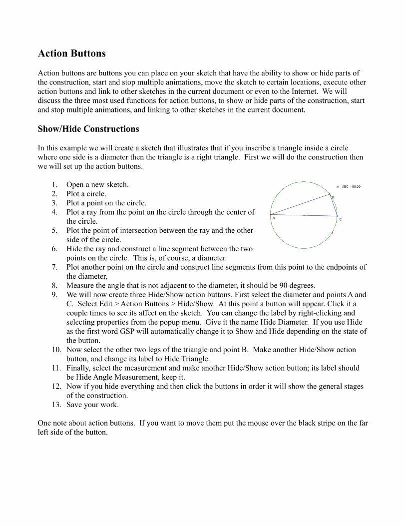
In this example we will create a sketch that illustrates that if you inscribe a triangle inside a circle where one side is a diameter then the triangle is a right triangle. First we will do the construction then we will set up the action buttons.

1. Open a new sketch. 2. Plot a circle. 3. Plot a point on the circle. 4. Plot a ray from the point on the circle through the center of

the circle. 5. Plot the point of intersection between the ray and the other

side of the circle. 6. Hide the ray and construct a line segment between the two

points on the circle. This is, of course, a diameter. 7. Plot another point on the circle and construct line segments from this point to the endpoints of

the diameter, 8. Measure the angle that is not adjacent to the diameter, it should be 90 degrees. 9. We will now create three Hide/Show action buttons. First select the diameter and points A and

C. Select Edit > Action Buttons > Hide/Show. At this point a button will appear. Click it a couple times to see its affect on the sketch. You can change the label by right-clicking and selecting properties from the popup menu. Give it the name Hide Diameter. If you use Hide as the first word GSP will automatically change it to Show and Hide depending on the state of the button.

10. Now select the other two legs of the triangle and point B. Make another Hide/Show action button, and change its label to Hide Triangle.

11. Finally, select the measurement and make another Hide/Show action button; its label should be Hide Angle Measurement, keep it.

12. Now if you hide everything and then click the buttons in order it will show the general stages of the construction.

13. Save your work.

One note about action buttons. If you want to move them put the mouse over the black stripe on the far left side of the button.

m ∠ ABC = 90.00 °

CA

B

Start/Stop Animations

We will first do a simple example of an animation action button and then we will do a nifty example which will simulate the old spirograph.

1. Load in the Simpson Line sketch.2. Select the point on the circle which is not part of the

inscribed triangle.3. Select Edit > Action Buttons > Animation... At this point

the animation dialog will appear with one item in the animate display, which is to animate the point moving around the circle. Change the speed to fast and click OK. At this point an animate action button will appear.

4. Click the animation button several times to see it turn the animation off and on.

Spirograph Example

This example will simulate those old spirograph games we all know and love from childhood. It is similar to the above example but will animate two points with a single animate button. The construction is really not very complicated..

1. Open a new sketch. 2. Plot a circle. 3. Plot a point on that circle, label it as A. 4. Construct a ray from the center of the circle through A. 5. Plot a point on the ray that is outside the circle. 6. Construct another circle with this last point as its center and its

circumference point is A. 7. Plot a point on this second circle, label it as B. 8. Select A and B then select Edit > Action Buttons > Animation...

At this point the animation dialog will appear with two items in the animate display. Change the speed to fast for both of them by selecting one of them in the list and selecting fast and then selecting the other and selecting fast, then click OK. At this point an animate action button will appear.

9. Click the animation button several times to see it turn the animation off and on. 10. This is nice but it does not give the spirograph image we were expecting. Select B and turn on

tracing for that point. Then turn on the animation.

A

B

Multiple Documents and Links to Them.

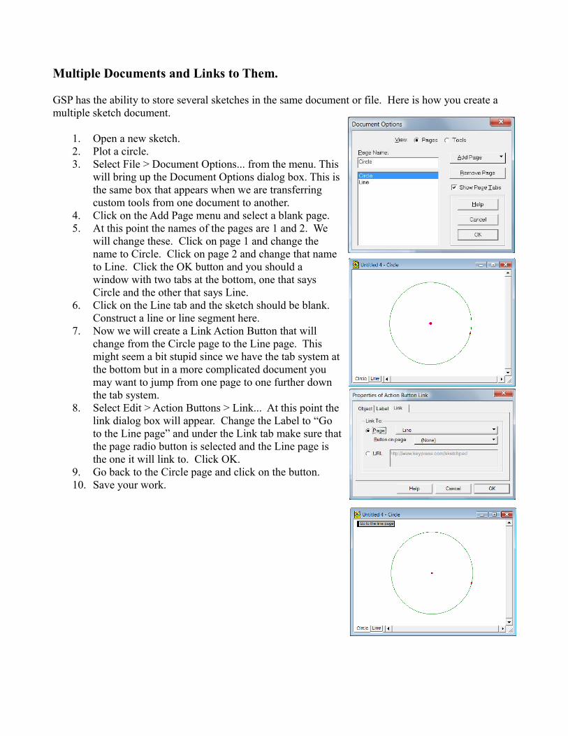
GSP has the ability to store several sketches in the same document or file. Here is how you create a multiple sketch document.

1. Open a new sketch. 2. Plot a circle. 3. Select File > Document Options... from the menu. This

will bring up the Document Options dialog box. This is the same box that appears when we are transferring custom tools from one document to another.

4. Click on the Add Page menu and select a blank page. 5. At this point the names of the pages are 1 and 2. We

will change these. Click on page 1 and change the name to Circle. Click on page 2 and change that name to Line. Click the OK button and you should a window with two tabs at the bottom, one that says Circle and the other that says Line.

6. Click on the Line tab and the sketch should be blank. Construct a line or line segment here.

7. Now we will create a Link Action Button that will change from the Circle page to the Line page. This might seem a bit stupid since we have the tab system at the bottom but in a more complicated document you may want to jump from one page to one further down the tab system.

8. Select Edit > Action Buttons > Link... At this point the link dialog box will appear. Change the Label to “Go to the Line page” and under the Link tab make sure that the page radio button is selected and the Line page is the one it will link to. Click OK.

9. Go back to the Circle page and click on the button. 10. Save your work.

Slider Construction and Locking Objects to the Sketch.

A slider is simply a “tool” that allows you to select a value by sliding a pointer along a line and link this value to other parts of the sketch. Sliders are not built-in objects in BSP so you need to create them yourself. There are several ways you can create a slider but we will look at only two. The first way is to simply place a point on the x-axis and use the x coordinate as the slider value and the second (which will not need a coordinate system) is to put a point on a line segment and do a short calculation to create a slider that starts at a value a and ends at a value b.

Sliders as Points on the x-axis

1. Open a new sketch. 2. Select Graph > Define Coordinate System to put the grid on the sketch. 3. Select Graph > Grid Form > Square Grid if it is not already checked. 4. Plot two points on the x-axis. Label one of them M and the other B. 5. Select the points and select Measure > Abscissa (x) from the menu. This puts the x value of

the points in the upper left as measurements we can use. 6. We will discuss plotting functions in more detail later but for now simply select Graph > Plot

New Function from the menu. At this point the calculation dialog box will appear. Click the xM measurement, then the *, then x, then + then the xB measurement and finally click OK. This will plot the line y = mx+b where m and b are the points on the x-axis.

7. Do a drag test with the M and B points to see the result. 8. Save your work/

6

5

4

3

2

1

-1

-2

-3

-4

-5

-6

-12 -10 -8 -6 -4 -2 2 4 6 8 10 12

f x( ) = xM ⋅ x+xB

xB = 2.52

xM = -1.69

M B

General Slider Construction

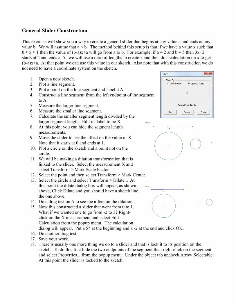
This exercise will show you a way to create a general slider that begins at any value a and ends at any value b. We will assume that a < b. The method behind this setup is that if we have a value x suck that 0 ≤ x ≤ 1 then the value of (b-a)x+a will go from a to b. For example, if a = 2 and b = 5 then 3x+2 starts at 2 and ends at 5. we will use a ratio of lengths to create x and then do a calculation on x to get (b-a)x+a. At that point we can use this value in our sketch. Also note that with this construction we do not need to have a coordinate system on the sketch.

1. Open a new sketch. 2. Plot a line segment. 3. Plot a point on the line segment and label it A. 4. Construct a line segment from the left endpoint of the segment

to A. 5. Measure the larger line segment. 6. Measure the smaller line segment. 7. Calculate the smaller segment length divided by the

larger segment length. Edit its label to be X. 8. At this point you can hide the segment length

measurements. 9. Move the slider to see the affect on the value of X.

Note that it starts at 0 and ends at 1. 10. Plot a circle on the sketch and a point not on the

circle. 11. We will be making a dilation transformation that is

linked to the slider. Select the measurement X and select Transform > Mark Scale Factor.

12. Select the point and then select Transform > Mark Center. 13. Select the circle and select Transform > Dilate... At

this point the dilate dialog box will appear, as shown above, Click Dilate and you should have a sketch line the one above.

14. Do a drag test on A to see the affect on the dilation. 15. Now this constructed a slider that went from 0 to 1.

What if we wanted one to go from -2 to 3? Right-click on the X measurement and select Edit Calculation from the popup menu. The calculation dialog will appear. Put a 5* at the beginning and a -2 at the end and click OK.

16. Do another drag test. 17. Save your work. 18. There is usually one more thing we do to a slider and that is lock it to its position on the

sketch. To do this first hide the two endpoints of the segment then right-click on the segment and select Properties... from the popup menu. Under the object tab uncheck Arrow Selectable. At this point the slider is locked to the sketch.

X = 0.37

A

X = -0.26

A

Split/Merge Option

The Split/Merge option allows you to combine objects and split objects that are linked in some way. It is useful if you are creating a complicated sketch and notice that you needed two segment to have a point in common, instead of starting over or backtracking you might be able to simply combine two points.

1. Open a new sketch. 2. Plot two line segments. 3. Select the left endpoints of each of the segments. 4. Select Edit > Merge Points from the menu and the two

points will merge into one. 5. Do a drag test. 6. Now select the common point you just merged and select

Edit > Split Point and the two line segments will no longer be connected.

Tessellations

Loosely speaking, a tessellation of the plane is a covering of the plane by a finite number of non-overlapping congruent shapes. Some of the most famous tessellations were produced by the artist M. C. Escher. We will not be producing anything close to his work but we will use GSP to create a couple tessellations that can be dynamically changed.

Glide Example

In a glide (or translation) tessellation we start with a single shape and repeatedly translate it by the same amount infinitely often. So it seems that the object that we are translating will need to have one side fit perfectly into the opposite side. The way we are going to construct this is by starting with a parallelogram, manipulate one side of it and then copy that manipulation (with a translation) to the opposite side. Once this has been done for all sides we will paste copies of them together.

1. Open a new sketch. 2. Construct two line segments that meet at a point. Label the points

A, B, and C. 3. Click on A followed by B. 4. Select Transform > Mark Vector 5. Select the AC segment and C, but not A. 6. Select Transform > Translate, when the dialog box appears make

sure it says to translate from Point A to Point B and click the Translate button. This will create a line segment BC' that is the same length and parallel to AC.

7. Construct a segment from C to C'. At this point you have a parallelogram.

8. Do a drag test to make sure it always stays a parallelogram. 9. Now construct a series of three or four line segments from A to C. None of the points need to

A

C

B

C'

A

C

B

be on the segment AC. 10. Select the segments you just created along with their endpoints, except for A and C. 11. Select Transform > Translate, when the dialog box appears make sure it says to translate from

Point A to Point B and click the Translate button. This will create a copy of the segments on the line segment BC'.

12. Do a drag test. 13. Now construct a series of three or four line segments from A to B. None of the points need to

be on the segment AB. 14. Select A followed by C and then select Transform > Mark Vector. 15. Select the segments you just created along with their

endpoints, except for A and B. 16. Select Transform > Translate, when the dialog box appears

make sure it says to translate from Point A to Point C and click the Translate button. This will create a copy of the segments on the line segment CC'. You should have something similar to the image at the right.

17. Do a drag test. 18. What we intend to do is use the jagged edged object above to

tile the plane. Since we made the opposite sides identical the pieces should fit exactly into each other.

19. Select all of the points in the sketch in a counter-clockwise manner.

20. Select Construct > Polygon Interior. 21. Now we start copying and pasting, so to speak. Select the

interior and nothing else. Since we still have the AC vector marked, select Transform > Translate, when the dialog box appears make sure it says to translate from Point A to Point C and click the Translate button. At this point another copy of the interior will appear above the original. Unfortunately it is the same color, change the color of the new area.

22. Now select the new area and select Transform > Translate again. Change the color of the new area.

23. Do the same with the new areas until most of the vertical distance of your sketch is filled.

24. Now we copy horizontally. Select the points A followed by B and then select Transform > Mark Vector.

25. Select all of the areas in the sketch and then select Transformation > Translate. Make sure it says to translate from Point A to Point B and click the Translate button. This will create another column of things.

26. Select the new column and do another translation. Repeat until most of the horizontal distance of your sketch is filled. Note that the colors of the areas do not alternate, change the coloring to make the tiling more readable.


C'

A

C

B

C'

A

C

B

C'

A

C

B

C'

A

C

B

Rotation Example

In a rotation tessellation we use rotations to tile the plane instead (or in addition to) translations.

1. Open a new sketch. 2. Construct an equilateral triangle and label the points A, B and C. 3. Now construct a series of three or four line segments from A to B.

None of the points need to be on the segment AB. 4. Select A and then select Transform > Mark Center. 5. Select the segments and ponts you created from A to B but do not

select A or B. 6. Select Transform > Rotate and rotate by the fixed angle of 60 degrees.

At this point the sketch should look something like the one to the right. 7. Do a drag test. 8. Construct the midpoint of BC and call it D. 9. Construct two line segments from C to D with one common point. As

in the image to the right. 10. Construct a circle with center D and edge point the one just created. 11. Construct a ray from the edge point through D. 12. Construct the point of intersection of the ray and the other side of the

circle. As in the image to the right. 13. Hide the circle and the ray. 14. Construct segments from D to the intersection point and the

intersection point to B. 15. Do a drag test. 16. Select all of the points in counter-clockwise order. 17. Select Construct > Polygon Interior from the menu. 18. Now it is time to tessellate. Select the area you just created and then

select Transform > Rotate... The point A should still be the one that is marked and rotate by 60 degrees.

19. Rotate the new area by 60 degrees and so on until you are finished with one revolution. As with the last example recolor the alternate areas to make the tiling more visible.

20. Do a drag test. 21. Now mark D as a rotation center. Select all six areas and then rotate

around D by 180 degrees. 22. Now rotate the six new areas around C by 120 degrees and those same

six by -120 degrees around B. we could continue to fill the plane but we will stop here.

23. Save your work and do a drag test.

C

A B

D

C

A B

D

C

A B

D

C

A B

D

C

A B

Constructions on Images: Golden Ratio Example.

GSP has the ability to place an image on a sketch which allows you to do geometric constructions on real-life objects. What we are going to do is measure the ratio of the height of the Parthenon verses its width.

1. Open the gold05sm.jpg file in Paint or some other graphics program.

2. Select the entire image and copy it to the clipboard.3. Open a new sketch.4. Press Control+V to paste the image into GSP.5. Since the Parthenon is in not so good shape we need to first

reconstruct the roof. Construct an isosceles triangle for the roof where one side is along the top support structure and the other two sides are where the roof was centuries ago.

6. Create another line segment at the base of the building.7. Drop a perpendicular from the top of the roof to the base line. 8. Construct the point of intersection between the perpendicular

and the base.9. Hide the perpendicular and replace it with a line segment. 10. Measure the base length and the height and finally calculate

the base divided by the height. You should come out with about 1.62, give or take. This exercise is prone to error. This number is an approximation to the Golden Ratio which is

152

B

E

C D

A

Functions

GSP has facilities for exploring functions so GSP can easily be used for demonstrations and explorations in other areas of mathematics such as algebra, trigonometry and calculus.

Plotting Simple Functions.

In this example we will plot just a few simple functions.

1. Open a new sketch. 2. Select Graph > Plot New Function. At this point the New

Function dialog box will appear, pictured to the right. 3. Like the calculation dialog box GSP does not let you make a

syntax error by only allowing you to select the keys that would create valid syntax. There are a couple menus to the right. The Values menu lets you pick the variable x (which is also a key), e and π. The Functions menu contains a few standard functions like sine cosine and square root. The Equation menu allows you to select between y = f(x) or x = f(y) form for rectangular coordinates and r = f(θ) or θ = f(r) for polar coordinates. Input the function x*3-4*x^2+3*x-1 and click OK. You should see something similar to the following graph.

Functions in GSP are not as functional as geometric objects, that is, there are fewer options you have when working with functions. Although, you can plot points on them and link lines and circles to these points so from a pedagogical point of view there are many functional properties you can demonstrate and explore using GSP.

Integrating Sliders with Functions

One standard exercise many teachers like to do with dynamic software is to plot a general function, like ax^2+bx+c and alter the values of a, b, and c dynamically to see the affect each parameter has on the graph of the function. If you have not done the slider exercise above you should complete this before continuing with this exercise.

1. Open a new sketch. 2. Create three general sliders that range between -5 and 5 and label the final result calculation as

a, b and c. 3. Select Graph > Plot New Function. Input the function a*x^2+b*x+c. When you want a, b and

c you simply need to click on the calculation displayed on the sketch. Click OK when you are finished. You should get the image below.


6

5

4

3

2

1

-1

-2

-3

-4

-5

-6

-12 -10 -8 -6 -4 -2 2 4 6 8 10 12

f x( ) = a ⋅x2+b ⋅ x+c

c = 1.14

b = -2.22

a = -0.42A

B

C

Derivatives and Tangent lines

For this exercise we will plot a tangent line to the cubic function we graphed above.

1. Open up the file you saved the cubic function plot to and resave it under a different name. 2. We wish to plot a tangent line to the curve. So we will need a point of tangency. Plot a point on

the function. 3. Do a drag test to make sure the point is attached to the function. 4. We will also need the derivative of the function. Select the function definition and not the

graph. The function definition is in the upper left corner of the sketch, like a measurement. Then select Graph > Derivative. The derivative will appear in the upper left as well.

5. We will also need the x coordinate of the point of tangency. Select the point and then select Measure > Abscissa (x) from the menu. This will also appear in the upper left as xA.

6. Now we are ready for the tangent line. In GSP the tangent line is really not a line it is the plot of a function. As we know from calculus, the equation of a tangent line is f'(a)(x-a)+f(a) where a is the x coordinate of the point of tangency. Select Graph > Plot New Function and input the following.(a) Click on the derivative definition.(b) Click on xA.(c) Move the cursor to the end.(d) Click on the *(e) Click on the ((f) Click on the x(g) Click on the -(h) Click on xA.(i) Click on the )(j) Click on the +(k) Click on the function definition.(l) Click on xA.(m)Click OK

7. At this point you should have a tangent line to the curve through the point you plotted on the curve. Do a drag test.

8. One result of the fact that the tangent line is a GSP function is that we cannot do some simple measurements on it like we can with a line. For example if you select the tangent line and then try to measure its slope you will not be able to. So if you want the students to see a slope relationship then they would need to do the f'(a) calculation.

Iteration

GSP has the ability to iterate transformations. To set up an iteration you first create a single instance of the transformation then to iterate the process you tell GSP what the initial object is, what the first iteration should be and how many iterations to do. We will do a simple example of constructing a set of points that spiral around a fixed point. To create a spiral (specifically a logarithmic spiral) we start with a point, we then rotate it by a fixed amount about a fixed point and increase its distance from the same fixed point by a fixed factor. The way we can do this in GSP is to do two transformations on a point and then iterate that composition of transformations. Here is the construction.

1. Open a new sketch. 2. Plot two points and label them as A and B. 3. Select A and then select Transform > Mark Center. This will

be the point that the spiral will spin around. 4. Select A and then B in that order. Then select Transform >

Mark Vector. This will be the vector that we increase so that the spiral is not a circle.

5. Select B and select Transform > Rotate... put 5 in the degrees box and click the Rotate button. This will create a point rotated 5 degrees around A from B. This is actually just an intermediate step and will be hidden later.

6. Select this new point and select Transform > Dilate... put 1.05 in the numerator of the ratio and 1.0 in the denominator of the ratio. As in the image in the upper right. At this point your sketch should look like the image to the right. If the points around B are difficult to distinguish move B away from A and the points should separate slightly.

7. Hide the point that was produced by the intermediate step of just the rotation.

8. Select B. 9. Select Transform > Iterate. At this point the Iterate dialog box

will appear, pictured to the right. To fill in the First Image box simply click on the point that resulted from both the rotation and the dilation. It will probably be called B' and that will appear in the First Image box. Now hold down the + key until the number of iterations is 100 and then click Iterate.

10. Since B was far from A the spiral probably does not look very good. Move B closer to A for a better picture.

A

B

A B

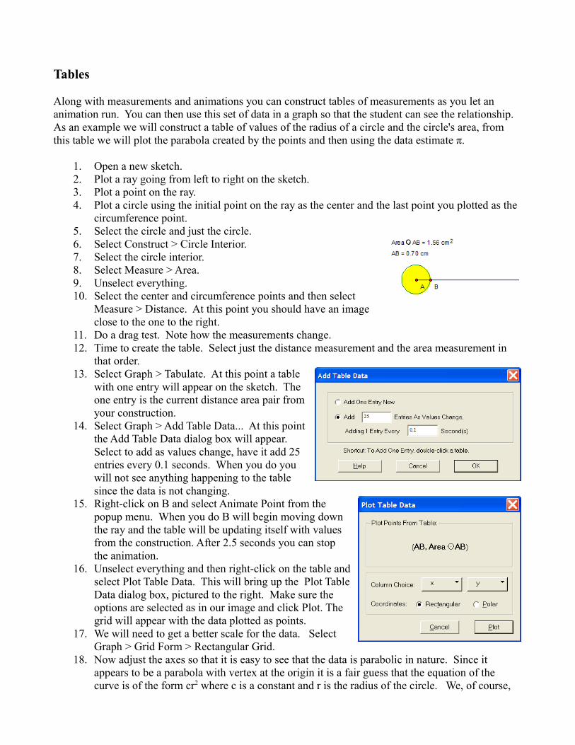
Tables

Along with measurements and animations you can construct tables of measurements as you let an animation run. You can then use this set of data in a graph so that the student can see the relationship. As an example we will construct a table of values of the radius of a circle and the circle's area, from this table we will plot the parabola created by the points and then using the data estimate π.

1. Open a new sketch. 2. Plot a ray going from left to right on the sketch. 3. Plot a point on the ray. 4. Plot a circle using the initial point on the ray as the center and the last point you plotted as the

circumference point. 5. Select the circle and just the circle. 6. Select Construct > Circle Interior. 7. Select the circle interior. 8. Select Measure > Area. 9. Unselect everything. 10. Select the center and circumference points and then select

Measure > Distance. At this point you should have an image close to the one to the right.

11. Do a drag test. Note how the measurements change. 12. Time to create the table. Select just the distance measurement and the area measurement in

that order. 13. Select Graph > Tabulate. At this point a table

with one entry will appear on the sketch. The one entry is the current distance area pair from your construction.

14. Select Graph > Add Table Data... At this point the Add Table Data dialog box will appear. Select to add as values change, have it add 25 entries every 0.1 seconds. When you do you will not see anything happening to the table since the data is not changing.

15. Right-click on B and select Animate Point from the popup menu. When you do B will begin moving down the ray and the table will be updating itself with values from the construction. After 2.5 seconds you can stop the animation.

16. Unselect everything and then right-click on the table and select Plot Table Data. This will bring up the Plot Table Data dialog box, pictured to the right. Make sure the options are selected as in our image and click Plot. The grid will appear with the data plotted as points.

17. We will need to get a better scale for the data. Select Graph > Grid Form > Rectangular Grid.

18. Now adjust the axes so that it is easy to see that the data is parabolic in nature. Since it appears to be a parabola with vertex at the origin it is a fair guess that the equation of the curve is of the form cr2 where c is a constant and r is the radius of the circle. We, of course,

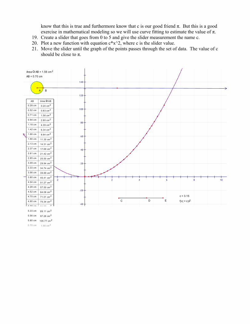
know that this is true and furthermore know that c is our good friend π. But this is a good exercise in mathematical modeling so we will use curve fitting to estimate the value of π.

19. Create a slider that goes from 0 to 5 and give the slider measurement the name c. 20. Plot a new function with equation c*x^2, where c is the slider value. 21. Move the slider until the graph of the points passes through the set of data. The value of c

should be close to π.

140

120

100

80

60

40

20

-2 0

-4 0

-4 -2 2 4 6 8 10

AB Area AB

0.28 cm 0.24 cm 2

0.52 cm 0.83 cm 2

0.71 cm 1.56 cm 2

0.94 cm 2.80 cm 2

1.18 cm 4.39 cm 2

1.42 cm 6.34 cm 2

1.66 cm 8.64 cm 2

1.90 cm 11.30 cm 2

2.13 cm 14.31 cm 2

2.37 cm 17.69 cm 2

2.61 cm 21.42 cm 2

2.85 cm 25.50 cm 2

3.09 cm 29.94 cm 2

3.33 cm 34.74 cm 2

3.56 cm 39.89 cm 2

3.80 cm 45.41 cm 2

4.04 cm 51.27 cm 2

4.28 cm 57.50 cm 2

4.52 cm 64.08 cm 2

4.75 cm 71.01 cm 2

4.90 cm 75.34 cm 2

5.09 cm 81.32 cm 2

5.33 cm 89.11 cm 2

5.56 cm 97.26 cm 2

5.80 cm 105.77 cm 2

0.70 cm 1.56 cm 2

f x( ) = c⋅ x2

c = 3.15

AB = 0.70 cm

Area AB = 1.56 cm 2

A

C E

B

D

JavaSketchpad (JSP)

JavaSketchpad (JSP) is software that lets you interact with — or publish — sketches from The Geometer's Sketchpad on the Internet. The Geometer's Sketchpad is a Dynamic Geometry exploration environment available for Macintosh and PC computers from Key Curriculum Press. You can use JavaSketchpad to share your geometry work (or your students' work) with people who may not have desktop Sketchpad or who use computers that can't access desktop Sketchpad (like most UNIX machines). You can use JavaSketchpad to distribute interactive, Dynamic Geometry activities and curricula over the Internet. Advanced users, programmers, and mathematical researchers can even use JavaSketchpad to add Dynamic Geometry visualization to other software or problem contexts.

JavaSketchpad and Geometer's Sketchpad have their differences. There are items that can be placed on a Geometer's Sketchpad sketch (such as function graphs) which will not be displayed in JSP. There are also some things in JSP that cannot be done in GSP and these require a little more technical skill with HTML. If you try to save a JSP (that is HTML) file that uses components that JSP will not understand GSP will give you a warning to that affect.

In general, when your GSP sketch contains just the elements that JSP can understand you only need to save your GSP sketch as an HTML page and you now have a web page that will let the user dynamically use the sketch (just like they can with GSP). We will go over a simple example shortly but if you are interested in investigating this further you can start with the JSP web site at

http://www.dynamicgeometry.com/JavaSketchpad/About_JavaSketchpad.html

1. Open the Simpson Line file you created above.2. Select File > Save As from the menu.3. In the Save As Type area select HTML/Java Sketchpad Document.4. Change the filename to SimpsonLine.htm (if it is not already input as that).5. Click Save.6. Now copy the entire jsp folder to the same folder that you saved SimpsonLine.htm to.7. Open the SimpsonLine.htm file in your favorite web browser. 8. Do a drag test on the sketch.

Note that you can open the SimpsonLine.htm file in HTML editing programs like MS Frontpage and add commentary to the sketch.

GeoGebra: Similarities and Differences with GSP.

GeoGebra is dynamic mathematics software that joins geometry, algebra and calculus. It is developed for learning and teaching mathematics in schools by Markus Hohenwarter and an international team of programmers.

Both GeoGebra and GSP are dynamic and they both offer geometric construction tools, measurement tools and transformation tools. While GSP places many of these as menu option GeoGebra has them as special tools in the toolbar. GeoGebra is freeware unlike GSP,

The main advantages of GSP over GeoGebra are

1. GSP has a nice calculation dialog box interface.2. GSP has the ability to create action buttons.3. GSP has a cleaner interface for simple animations. 4. GSP has the ability to iterate transformations.

The main advantages of GeoGebra over GSP, besides being free, are

1. GeoGebra has a better algebraic interface for explorations concerning trigonometry and calculus.

2. GeoGebra has a built-in slider tool which easily integrates with other objects.3. GeoGebra is able to do transformations on graphic images.4. GeoGebra has more built-in geometric and algebraic functions.5. GeoGebra has an easier show/hide interface through their algebra window.6. GeoGebra has customizable toolbars.7. GeoGebra has more specific tools for conic sections, tangent lines, circles, sectors and arcs

between points, best fit lines, ...8. GeoGebra has a fully functional web interface, including adding objects as well as clipboard

and file transfer. It does not have the limitations that JSP has with GSP files.9. GeoGebra has a spreadsheet interface for easy data collection, data transfer and graphing.10. GeoGebra has a construction protocol interface to view the entire construction process.

In general, and in my opinion, GeoGebra has more functionality that makes more advanced constructions and its integration into higher level courses much easier. GSP on the other hand is marginally easier to use and has a much nicer interface for animations.

Links of Interest

• http://www.keypress.com/ – Key Curriculum Press• http://www.dynamicgeometry.com/ – Geometer's Sketchpad® Resource Center• http://www.dynamicgeometry.com/JavaSketchpad.html – JavaSketchpad• http://elearning.phiman.ac.th/~e_data/sketchpad/keypress/www.keypress.com/sketchpad/genera

l_resources/classroom_activities/index.html – Classroom Activities from key press.• http://whistleralley.com/GSP/sketchpad.htm – The Geometer's Sketchpad Workshop by Paul

Kunkel • http://mathforum.org/sketchpad/intro/gsp.introlab.html – The Geometer's Sketchpad

Introductory Lab• http://mathforum.org/sketchpad/sketchpad.html – The Geometer's Sketchpad Math Forum

Classroom Resources• http://www.geom.uiuc.edu/~demo5337/Group6/ – The Geometer's Sketchpad: A workshop

developed for the Saint Paul Public Schools at The Geometry Center, University of Minnesota• http://connectedmath.msu.edu/ – Connected Mathematics Project (CMP) at Michigan State

University.• http://humboldtsr.spps.org/Sketchpad.html – Geometer Sketchpad Tutorials and Resources • http://illuminations.nctm.org/Lessons.aspx – Illuminations: Resources for Teaching

Mathematics – NCTM• http://www.wpunj.edu/icip/itm/Lessonpl/sketch/sketch.html – Lesson Plans for the Geometer's

Sketchpad• http://www.mste.uiuc.edu/courses/ci407su01/students/south/ychen17/termproject/geometer.html

– Dynamic Geometer's Sketchpad• http://mathforum.org/library/selected_sites/collection.geometry.html – The Math Forum Drexel

University.• http://www.ettc.net/techfellow/sketch.htm – Geometer's Sketchpad, at The Virtual Institute for

teachers.• http://www.wiley.com/college/musser/CL_0471263796_S/sketchpad/sketchpad_tutorial/ –

Using Geometer's Sketchpad ® Tutorial Prepared by Armando Martinez-Cruz, California State University, Fullerton

• http://www.mathbits.com/MathBits/GSP/Gsp.htm – MathBits• http://www.joelduffin.com/wiki/index.php/Geometer's_Sketchpad – A personal wiki.• http://en.wikipedia.org/wiki/The_Geometer's_Sketchpad – GSP wiki.• http://en.wikipedia.org/wiki/Interactive_geometry_software – Interactive geometry software

wiki• http://faculty.kutztown.edu/schaeffe/GSP/GSP.html – Geometer's Sketchpad Lessons: Prepared

by students in R.S. Scheffer's Methods of Teaching Secondary Mathematics class over the past few semesters at Kutztown University, PA.

• http://highered.mcgraw-hill.com/sites/0073022845/student_view0/geometer_s_sketchpad.html – Bennett-Burton-Nelson package from McGraw-Hill Higher Education

• http://jwilson.coe.uga.edu/GSP.Lesson.Folder/GSP.Lesson.html – Jim WilsonDepartment of Mathematics Education University of Georgia

• http://www.teacherlink.org/content/math/activities/sketchpad.html – The Geometer's Sketchpad Activities Center for technology in teacher education University of Virginia.

http://www.keypress.com/

http://www.teacherlink.org/content/math/activities/sketchpad.html

http://jwilson.coe.uga.edu/GSP.Lesson.Folder/GSP.Lesson.html

http://highered.mcgraw-hill.com/sites/0073022845/student_view0/geometer_s_sketchpad.html

http://faculty.kutztown.edu/schaeffe/GSP/GSP.html

http://en.wikipedia.org/wiki/Interactive_geometry_software

http://en.wikipedia.org/wiki/The_Geometer's_Sketchpad

http://www.joelduffin.com/wiki/index.php/Geometer's_Sketchpad

http://www.mathbits.com/MathBits/GSP/Gsp.htm

http://www.wiley.com/college/musser/CL_0471263796_S/sketchpad/sketchpad_tutorial/

http://www.ettc.net/techfellow/sketch.htm

http://mathforum.org/library/selected_sites/collection.geometry.html

http://www.mste.uiuc.edu/courses/ci407su01/students/south/ychen17/termproject/geometer.html

http://www.wpunj.edu/icip/itm/Lessonpl/sketch/sketch.html

http://illuminations.nctm.org/Lessons.aspx

http://humboldtsr.spps.org/Sketchpad.html

http://connectedmath.msu.edu/

http://www.geom.uiuc.edu/~demo5337/Group6/

http://mathforum.org/sketchpad/sketchpad.html

http://mathforum.org/sketchpad/intro/gsp.introlab.html

http://whistleralley.com/GSP/sketchpad.htm

http://elearning.phiman.ac.th/~e_data/sketchpad/keypress/www.keypress.com/sketchpad/general_resources/classroom_activities/index.html

http://elearning.phiman.ac.th/~e_data/sketchpad/keypress/www.keypress.com/sketchpad/general_resources/classroom_activities/index.html

http://www.dynamicgeometry.com/JavaSketchpad.html

http://www.dynamicgeometry.com/

• http://www.mrhayden.com/gsp.php – Geometer's Sketchpad Activities for middle school students.

Similar Freeware Packages

• http://www.geogebra.org/cms/ – GeoGebra homepage.• http://www.geogebra.org/en/wiki/index.php/Main_Page – GeoGebra wiki • http://www.geogebra.org/forum/index.php – GeoGebra User Forum • http://math.exeter.edu/rparris/ – Peanut Software packages

http://math.exeter.edu/rparris/

http://www.geogebra.org/forum/index.php

http://www.geogebra.org/en/wiki/index.php/Main_Page

http://www.geogebra.org/cms/

http://www.mrhayden.com/gsp.php

Geometer's Sketchpad Workshop - Salisbury...

Documents

Transcript of Geometer's Sketchpad Workshop - Salisbury...