1

Drawing Logarithmic Curves with

Geometer's Sketchpad: A Method Inspired by Historical Sources

David Dennis

&

Jere Confrey

Mailing Address: Dr. David Dennis 4249 Cedar Dr. San Bernardino, CA 92407 Tel: 909-883-0848 e-mail: david.dennis@earthlink.net

Originally published in J. King & D. Schattschneider (Eds.),

Geometry Turned On: Dynamic Software in Learning, Teaching and Research. Washington D.C.: Mathematical Association of America.

This research was funded by a grant from the National Science Foundation.

(Grant #9053590)

2

Drawing Logarithmic Curves with Geometer's Sketchpad: A Method Inspired by Historical Sources

David Dennis

& Jere Confrey

Abstract: We start by describing a mechanical linkage device from Descartes' Geometry which draws a series of curves which can locate an arbitrary number of geometric means between any two lengths. Using this linkage combined with Napier's original conception of logarithms as covariation between geometric and arithmetic sequences, one can then construct arbitrarily dense sets of points on any log curve. When this construction is created on Geometer's Sketchpad one obtains a family of curves with two physically adjustable parameters, which allow any geometric sequence to be mapped against any arithmetic sequence. The derivative of any logarithm is then obtained using only similar triangles, and other geometric properties are investigated, such as the constant subtangent of exponential curves. Related educational issues are discussed.

Introduction:

In this article we first describe a mechanical linkage device from Descartes’ Geometry

(1637), for finding any number of geometric means. This linkage device draws a family

of curves which we will discuss briefly. We then employ Descartes' device as part of a

construction that will find any number of points, as densely as desired, on any

logarithmic or exponential curve. This second construction uses the dynamic

geometry software, Geometer's Sketchpad, in a modern adaptation of several historical

ideas, combined in ways that provide useful and enlightening curricular suggestions,

including an elementary approach to tangent slopes. Several important educational

and epistemological questions are raised by our approach, and we conclude by

discussing these.

Descartes' Construction of Geometric Means:

In the Geometry (1637), Descartes considered the problem of finding n mean

proportionals (i.e. geometric means) between any two lengths a and b (with a<b). To

do this one must find a sequence of lengths beginning with a and ending with b such

3

that the ratio of any two consecutive terms is constant. In modern algebraic language,

this means finding a sequence xo, x1 , . . . , xn+1 such that for some fixed ratio r, xk =

a.rk and xn+1 = b. Hence the terms of the sequence have a constant ratio of r, and form a

geometric sequence beginning with a and ending with b.

Descartes began, as always, with a geometric construction. He imagined a

series of rulers with square ends sliding along and pushing each other creating a series

of similar right triangles (see Figure 1, which is reproduced from an original 1637

edition of the Geometry). Let Y be the origin with A and B on a circle of radius a

centered at Y. The tangent to the circle at B intersects the line XY (the x-axis) at the

point C. As angle XYZ increases, C moves further to the right on the x-axis. The

vertical from C then intersects the line XY at D which is still further from the origin.

The triangles YBC, YCD, YDE, YEF, etc. are all similar, since they are all right triangles

that contain the angle XYZ. Hence we have YBYC = YC

YD = YDYE = YE

YF = . . .

Therefore the sequence of lengths a=YB, YC, YD, YE, YF, . . . form a geometric

sequence.

Figure 1

4

If we let a=1 and angle XYZ=60°, we form the sequence: 1,2,4,8,16,32,.....

If angle XYZ=45°, the sequence of lengths is: 1, 2 , 2, 2 2 , 4, 4 2 , 8, . . . which is a

refinement of the previous sequence. As angle XYZ decreases, we obtain increasingly

dense geometric sequences. In modern terms the relationship between the constant

ratio r and angle XYZ is given by the equation: sec(angle XYZ)= r. This relationship is

never mentioned in the Geometry. Descartes instead emphasized the curves traced by

the points D, F, and H as the angle XYZ is varied (shown in Figure 1 by the dotted

lines). These curves all have algebraic equations, as opposed to the secant which can

only be computed with some infinite process.

To solve the original problem of finding n mean proportionals between a and b,

Descartes suggested using the curves drawn by the device. For example, if two mean

proportionals are sought between a and b, mark off length b=YE on the line YZ (recall

a=YA). Next construct the circle having diameter YE, and find its intersection (D) with

the first of these curves (see Figure 1). Then drop the vertical line from that point (D)

to YZ, to locate the point C. YC and YD will then be the desired mean proportionals.

This method uses the curve drawn by D to determine the appropriate angle of the

device so that the point E will fall on any specified length.

The equations of the curves traced by D, F, H, . . . can all be found by

successively substituting into the similarity relations upon which the device was built.

To find these equations one can proceed as follows. Let Y=(0,0), D=(x,y), and let YD=z.

Now z2= x2+y2, but one also knows that zx = xa . Hence z= x2

a , and therefore by

substitution one obtains, for the path of point D, the equation: x4 = a2 (x2 + y2).

Now let F=(x,y), and let YF=z. Now zx = xYD , hence YD = x

2z . One also knows

that xYD = YD

YC , so substituting and solving for YC one gets: YC = x3

z2 . Lastly one

knows that YDYC = YC

a , and hence: ax2z = x

6

z4 . Solving for z one obtains: z = 3 x4

a .

5

As before z2=x2+y2, so 3 x8

a2 = x2 + y2 . Cubing both sides one obtains, for the path of

point F, the equation: x8 = a2 ( x2 + y2 )3 .

In a similar fashion, one can find that an equation of the curve traced by the

point H is: x12 = a2 ( x2 + y2 )5 . Note that all of these curves pass through the point

A=(a,0), and that as one moves from one of these curves to the next the degree of the

equation always increases by four (on both sides of the equation). In the Geometry,

Descartes proposed a system which classified curves according to pairs of algebraic

degree, i.e. lines and conics form the first "genre" of curves; those with third and fourth

degree equations form the second "genre" of curves; and so on.1 In many examples,

Descartes found that iterating various forms of mechanical linkages tended to jack up

by twos the degrees of the equations of the curves. The curve traced by D is of his

second genre; the curve traced by F is of the fourth genre; etc. To get from any one of

these curves to the next one involves two perpendicular projections, each of which

raises by one the Cartesian genre of the curve.

Descartes, after stating that, "there is, I believe, no easier method of finding any

number of mean proportionals, nor one whose demonstration is clearer," (1637, p. 155)

goes on to criticize his own construction for using curves of a higher genre than is

necessary. Finding two mean proportionals, for example, is equivalent to solving a

cubic equation and can be accomplished by using only conic sections (first genre) while

the curve traced by D is of the second genre. The solution of cubics by intersecting

conics had been achieved in the thirteenth century by Omar Khayyam and was well

known in seventeenth century Europe (Joseph, 1991). Descartes spent much of the

latter part of the Geometry discussing the issue of finding curves of minimal genre

which will solve various geometry problems (1637).

1 This same classification by pairs of degrees is used in modern topology in the definition of the "genus" of a surface. Classification by pairs of algebraic degrees often makes more sense geometrically.

6

Descartes expounded an epistemological theory which sought a universal

structural science of measure which he called "mathesis universalis" (Lenoir, 1979).

Fundamental to his program was his classification of curves in geometry. He wanted

to expand the repertoire of curves that were allowed in geometry beyond the classical

restrictions to lines and circles, but he only wanted to include curves whose

construction he considered to be "clear and distinct" (Descartes, 1637). For him this

meant curves which could be drawn by linkages (i.e. devices employing only hinged

rods and pivots). Such curves could all be classified by his system according to pairs

of algebraic degrees, since the class of curves that can be drawn by linkages is exactly

those which have algebraic equations (Artobolevski, 1964). Algebraic curves were

called "geometrical” by Descartes because he wanted to expand the constructions

allowed in geometry to include those curves. All other curves he called "mechanical."

This distinction is equivalent to what Leibniz would latter call "algebraic" and

"transcendental" curves. Descartes viewed "mechanical" (i.e. transcendental) curves as

involving some combination of incommensurable actions. Examples that he

specifically mentioned are the spiral, quadratrix, and cycloid. These curves all involve

a combination of rotation and linear motion that cannot be connected and regulated by

some linkage. The drawing of such curves involves rolling a wheel or the unwinding

of string from a circle. Descartes was aware that such curves could not be classified by

his system. This is not to say that Descartes did not address himself to problems

concerning transcendental curves (see Dennis, 1995, for some of his thoughts on the

cycloid).

A Dynamic Construction of Logarithmic Curves:

In order to construct logarithmic curves, we must first define the term

"subtangent." Given a smooth curve and an axis line, for each point P on the curve let

T be the intersection of the tangent line to the curve at P and the axis, and let O be the

foot of the perpendicular from P to the axis (i.e. PO is the ordinate, see Figure 2). For

7

each point P the subtangent is then defined as the line segment TO. Throughout the

seventeenth century, such geometric entities were studied for symmetry and

invariance as the point P moved along the curve. Such investigations played a very

important role both in the study of curves and in the development of the concept of

functions (Arnol'd, 1990; Dennis & Confrey, 1995).

Figure 2

Two years after the publication of the Geometry Descartes addressed a problem

that was sent to him by De Beaune which asked for the construction of a curve in a

skewed coordinate system where the ratios of the subtangents to the ordinates are

everywhere equal to the ratio of the ordinates to a fixed segment, i.e. a type of

logarithmic curve, the requirement being equivalent to a first order differential

equation (Lenoir, 1979). Descartes generated a method for pointwise approximation of

this curve and also provided a detailed study of how the curve could be drawn by a

combination of motions with particular progressions of speeds. He then stated:

I suspect that these two movements are incommensurable to such an extent that it will never be possible for one to regulate the other exactly, and thus this curve is one of those which I excluded from my Geometry as being mechanical; hence I am not surprised that I

8

have not been able to solve the problem in any way other than I have given here, for it is not a geometrical line. (Descartes, quoted in Lenoir, 1979, p. 362)2

We will now proceed to construct pointwise approximations of logarithmic

curves, but we will not follow the particular example discussed in Descartes' letters to

De Beaune. That example turns out to have been a transformation of a logarithm

added to a linear function. We will instead construct standard logarithmic curves

using Descartes' device shown in Figure 1, together with the original conception of

logarithms by Napier as pairings of geometric and arithmetic sequences (Smith &

Confrey, 1994; Edwards, 1979).

This construction connects curve drawing with a covariational view of

functions. Covariation is essentially a viewing of tables of data that looks for methods

to simultaneously extend or interpolate values in both columns separately, rather than

looking for a rule which relates values in the first column to those in the second. This

approach to functions was central in the thinking of Leibniz (Leibniz, 1712) and has

been shown to be important in the thinking of students (Rizzuti, 1991; Confrey &

Smith, 1995).

Napier and others in the early seventeenth century made tables of logarithms by

placing arithmetic sequence alongside geometric sequences. They devised various

ways to make these tables dense (Edwards, 1979). These early approaches to

logarithms were entirely tabular and calculational and did not involve curves or

graphs. When Descartes constructed a curve as a solution to De Beaune's problem he

did not view the curve as a "logarithm." A fully flexible view that could go back and

forth between curves, tables and equations did not evolve until the end of the

2 For a fascinating social and philosophical analysis of why Descartes would adopt such an attitude see the article by Lenoir (1979). It certainly had nothing to do with his ability to contend with such problems.

9

seventeenth century, especially with respect to transcendental curves whose general

coordinates could only be found by using series expansions (Dennis & Confrey, 1993).

Our aim here is to provide modern students with a hands-on way to build

logarithmic and exponential curves through a series of simple geometric constructions

using Geometer's Sketchpad. From the standpoint of covariation there is little difference

between exponentials and logs. The pair of actions which builds one also builds the

other. We have constructed the following curves as logarithms, but the same

constructions could be viewed as exponentials, by simply repositioning the

constructive actions.

We start by building a computer simulation of Descartes' device for the

construction of geometric sequences with a=1 (see Figure 3). Let O be the origin and

let H be any point on the unit circle. By moving H around the circle the distances of

the labeled points from the origin will form geometric sequences with any common

ratio. That is if r = OG1, then r2=OH2, r3=OG3, r4=OH4, etc.

Figure 3

10

This construction can also be extended to the interior of the unit circle to obtain

segments whose lengths are the negative powers of r. Once again, as with the

preceding construction, the odd powers of r are on the horizontal while the even

powers of r are on the line OH. This can be seen, as before, by considering the series of

similar triangles with common vertex O (see Figure 4).

Figure 4

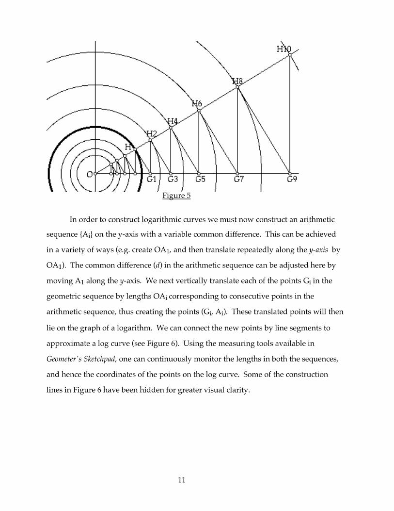
In order to get the entire geometric sequence on one line, we will now transfer

the lengths marked on the line OH onto the x-axis by using circles centered at O (see

Figure 5). Thus we now have a geometric sequence laid out on the x-axis whose

common ratio, or density, can be varied as the point H is rotated. The point where the

circle through H2 intersects the x-axis, we will name G2, likewise for H4, H6, etc. The

points on the x-axis that are inside the unit circle we will call G-1, G-2, . . . etc. where

the subscripts correspond to the powers of r that represent their distances from O.

11

Figure 5

In order to construct logarithmic curves we must now construct an arithmetic

sequence {Ai} on the y-axis with a variable common difference. This can be achieved

in a variety of ways (e.g. create OA1, and then translate repeatedly along the y-axis by

OA1). The common difference (d) in the arithmetic sequence can be adjusted here by

moving A1 along the y-axis. We next vertically translate each of the points Gi in the

geometric sequence by lengths OAi corresponding to consecutive points in the

arithmetic sequence, thus creating the points (Gi, Ai). These translated points will then

lie on the graph of a logarithm. We can connect the new points by line segments to

approximate a log curve (see Figure 6). Using the measuring tools available in

Geometer's Sketchpad, one can continuously monitor the lengths in both the sequences,

and hence the coordinates of the points on the log curve. Some of the construction

lines in Figure 6 have been hidden for greater visual clarity.

12

A1

A2

A3

A5

A6

A7

A8

A9

A-1

A-2

A-3

Figure 6

We now have an adjustable curve. By moving H around the unit circle or A1

along the y-axis, one can map any geometric sequence against any arithmetic sequence.

In Figure 6 the point H is adjusted so that G4=2, and the point A1 is adjusted so that

A4=1. Hence this curve is a graph of the log base 2.

13

By readjusting A1 so that A8=1 the curve shifts dynamically to become a graph

of the log base 4 (see Figure 7).

Figure 7

By readjusting the point H so that G8=3, one obtains a graph of the log base 3

(see Figure 8). Since the monitors are measuring to the hundredth of an inch, which is

smaller than a pixel, it is not always possible to get exactly the desired numbers by

simple direct actions (e.g. G8 reads 2.96 in Fig. 7). One can get around the pixel

problem by using the appropriate rescaling window commands, but for a first

experience this would decrease the sense of a direct physical approach, which we feel

is important for students.

14

Figure 8

It is fascinating to watch these curves flex and bend as the arithmetic and

geometric sequences are manipulated. Even when the points are quite broadly spaced,

as in Figure 6, the graphs look very smoothly curved, though they are all made up of

line segments. When the angle of H is increased, the geometric sequence spreads out

rapidly off of the screen. By scanning far to the right, it is instructive to see just how

incredibly flat log curves become.

When the arithmetic and geometric sequences are both spread out, the graphs

can eventually become "chunky" since the points are being connected with line

segments. However, by manipulating both sequences it is possible to increase the

density of points on any particular log graph without changing the base. For example,

we could create another graph of the log base 2 by setting A8=1, and G8=2 (see Figure

9). This is the same curve as the one in Figure 6, but with a much higher density of

15

constructed points. Descartes' device allows us to geometrically carry out the

calculational aims of Napier and other seventeenth century table makers. Geometric

sequences can be built as densely as one desires, and paired against any arithmetic

sequence.

Figure 9 An Investigation of the Slopes of Logarithmic Curves:

After looking at these log curves shift and bend dynamically, one can begin to

look carefully at the slopes of segments that join points on the curves. Several

interesting patterns come to light. If the slopes of segments that join consecutive

constructed points are used to approximate the tangent slope at a point, say for

example at (1,0), it is visually apparent that this calculation is not the best thing to use.

The slope between the nearest points to the right and left of a point gives a better

approximation of the tangent slope at that point. This is true for most curves, not just

16

the logarithm.3 Here, at (1,0), the best approach to the tangent slope is to calculate the

secant slope between G-1, and G1. Letting r equal the common ratio of the geometric

sequence, and d equal the common difference of the arithmetic sequence, we calculate

this slope as:

tangent slope at (1,0) ≈ 2d

r - 1r = 2rd

r2 -1

We will use k for this approximate slope at (1,0). Suppose we now approximate

in the same way the slope at any other point on the constructed curve. The

approximate tangent slope at (Gn, An)=(rn, nd) is found by computing the secant slope

between Gn-1, and Gn+1. The calculation yields:

tangent slope at (Gn, An) ≈ 2drn+1 - rn-1 = 1

rn . 2rdr2 -1 = k

rn

Here one has the approximate tangent slope at a point on a logarithmic curve written

as the function 1x times a constant k that is the slope of the curve at (1,0). Of course

these slopes are all approximations, but once the slope at (1,0) is approximated it can

be divided by the x-coordinate at any other point to get the corresponding slope

approximation at that point. By making the constructed points on the curve denser,

the approximations all improve by the same factor. Thus the essential derivative

property of logarithms is revealed without recourse to the usual formalisms of

calculus. In fact, even more is being displayed here than the usual derivative of a

logarithm. One sees that the all the slope approximations converge uniformly, as the

density of the constructed points is increased.

3 It is strange that when the derivative is developed in calculus classes, it is defined using secant slopes from the point in question, rather than around the point. It would seem that nobody is directly interested in secant slope approximations, except as an algebraic device from which to define a limit. The practical geometry of using secant slopes is ignored.

17

This constant k (=the slope at (1,0)) can be seen geometrically in another way. If

we view these curves and tangent constructions using the vertical axis (i.e. as

exponential functions), then we find that the subtangent is constant for all points along

the curve, and is always equal to k. This can be established algebraically from the

previous discussion, but it is nice to see it geometrically on the curve, and verify it

using the measurement capability of Geometer's Sketchpad. This is shown in Figure 10

for two different points on the log base three curve. The tangent lines and slope are

approximated by using the points adjacent to the one under consideration and the

accuracy is quite good (a calculator gives k=.910).

Figure 10

This constant subtangent property was at the heart of Descartes' discussion of

De Beaune's curve. The constant subtangent was the hallmark by which logarithmic

and exponential curves were recognized during the seventeenth century (Lenoir, 1979;

Arnol'd 1990). One way to think of this property is to imagine using Newton's method

to search for a root of an exponential curve. The method will march off to infinity at a

constant arithmetical rate, where the size of the steps will be the constant k.

In order to construct the natural logarithm, we want the slope k at (1,0) to be

equal to 1. This is the property from which Euler first derived the number "e" (Euler,

1748). Returning to the construction, with a measure that monitors the secant slope k

between G-1, and G1, we now rotate H until the slope measurement reads as close to 1

18

as possible. We have now constructed a close approximation to the graph of the

natural logarithm. The approximate slope at any point on the curve is the inverse of its

x-coordinate. Note that since A5 = 1, the value of G5 is approximately the number "e"

(see Figure 11).

Figure 11

This geometric construction of points on log curves achieves the goals set out by

Napier. It allows one to construct logarithms (and also exponents) as densely as one

desires. Of course Napier achieved these goals through interpolation schemes

(Edwards, 1979), and throughout the seventeenth century increasingly subtle methods

of table interpolation were developed, e.g. those of John Wallis (Dennis & Confrey,

1996). The story of these calculational techniques is a very important one leading

eventually to Newton's development of binomial expansions for fractional powers.

Euler routinely used Newton's binomial expansion techniques to calculate log tables to

19

over 20 decimal places (Euler, 1748). Theoretically the geometric construction has

unlimited accuracy, and this can be achieved through appropriate rescalings, but

directly using measuring capability of Geometer's Sketchpad, one is limited to at most

three decimal places.

Conclusions:

Our approach raises several general educational and epistemological questions:

1) How are tools and their actions related to mathematical language and symbols?

2) What notion of functions arises from constructions made with particular tools?

3) What are the educational and epistemic roles of mathematical history?

The first question is addressed in theoretical detail by Confrey (1993). She

suggests that effective education in mathematics must be approached as a balanced

dialogue between "grounded activity" and "systematic inquiry." New technological

tools, such as dynamic geometry software, help to populate the dialogue between

physical investigations and symbolic language, allowing it to flow with greater ease.

Confrey stresses the need for balance in this dialogue. All too often in our

mathematics curriculum, symbolic language is given a preeminent role, de-

emphasizing visual and physical activity, especially at more advanced levels. The

examples discussed in this paper demonstrate the value of striking a balance.

The most common notion of a function that is taught in mathematics is to see it

as a rule or process which computes or predicts one quantity from another, i.e. a

correspondence notion. These quantities are most often real numbers, and functions

can then be represented by graphing these quantities in the plane. Our investigations

employed two different conceptions of functions, which have both played important

historical roles. The first conception involved creating a curve as a primary object

through some kind of physical of geometric action, and only afterwards analyzing it by

means of the geometric properties of particular magnitudes, such as abscissas,

ordinates, and subtangents (Dennis, 1995). Algebra and equations then become

20

secondary representations of curves, rather than primary generators. The second

conception of functions that came into play in our constructions is "covariation"

(Confrey & Smith, 1995). This view sees functions as a pair of independent operations

on columns in a table, where one finds ways to simultaneously extend or interpolate

values on both sides of a table thus generating a correspondence when the columns are

paired in a given position.

Both of these conceptions of functions have played important roles in the

genesis of analytic geometry and calculus. Neither one is entirely reducible to the

current "definition" of a function. For example, in Descartes' Geometry, never once is a

curve created by plotting points from an equation. Descartes always began with a

physical or geometric way of generating a curve, and then by analyzing the actions

which produced the curve, he obtained equations. Curves were primary and gave rise

to equations only as a secondary representation. Equations allowed him to create a

taxonomy of curves (Lenoir, 1979). Furthermore, Leibniz originally created his

calculus notation from his many experiments with tables, where a covariational

approach was his fundamental form of generation (Leibniz, 1712).

These alternative conceptions of functions are not just awkward phases of

historical development which should be abandoned in light of more modern

developments. Quite the contrary, they provide ways of working which give

mathematicians a powerful flexibility. They can help to balance the dialogue between

the physical world and our attempts to represent it symbolically, especially when

combined with newly available tools, such as Geometer's Sketchpad.

We ask the reader to compare this investigation of logarithms with the

approaches more frequently taken in classrooms. Many students are introduced to

logarithms in a formal algebraic way, with no references to geometry or to table

construction. Such students often have no method for geometrically or numerically

constructing, even a square root. Such an approach leads, at best, only to a superficial

21

understanding of the grammar of logarithmic notation. There is no dialogue at all

between geometrical, numerical and algebraic experience.

Another approach that is frequently taken is to see logarithms as the

accumulated area under a hyperbola (usually y=1/x). This approach can provide

many fascinating insights that connect logarithms to both geometry and to the

numerical construction of tables. The study of hyperbolic area accumulation was

fundamental in the early work of Newton, but was always linked in his work to

extensions of the table interpolations of John Wallis. It was in this setting that Newton

created his first infinite binomial expansions (Dennis & Confrey, 1993; Edwards, 1979).

Although the hyperbolic area approach can create a fascinating and balanced dialogue,

it is not usually taken with students until they are already involved with calculus. The

fundamental theorem of calculus, for example, is usually invoked to show that the

hyperbolic area function must have a derivative of 1/x.

The approach that we have described here is strictly pre-calculus. It involves

only a systematic use of similar triangles, in a hands-on setting that is both visual,

physical, and geometric. It provides a specific form of grounded activity that allows

students to manipulate, extend, and interpolate both logarithms and continuous

exponents. Rather than using calculus to create a balanced dialogue, this approach

uses the dialogue to achieve some of the results of calculus in a very simple setting. It

highlights the power of iterated geometric similarity (Confrey, 1994).

Reading this paper cannot truly convey the feeling one gets while physically

manipulating the curves. The investigation of the slopes of log curves depends

logically only on the properties of a table which maps a geometric sequence against an

arithmetic sequence, but we did not notice this piece of algebra until many fluctuating

examples of log curves had appeared on the screen. The geometry can heighten the

intuition so that fruitful conjectures emerge. The power of suggestion should not be

underestimated. The association of rotation around the unit circle with the building of

22

logarithms is a wonderful foreshadowing of the connections between these functions

and the trigonometric functions, when extended to the complex numbers (Euler, 1748).

References: Arnol'd, V. I. (1990). Huygens & Barrow, Newton & Hooke. Boston: Birkhäuser Verlag Artobolevskii, I. I. (1964). Mechanisms for the Generation of Plane Curves. New York:

Macmillan Co. Confrey, J. (1993). The role of technology in reconceptualizing functions and algebra.

In Joanne Rossi Becker and Barbara J. Pence (eds.) Proceedings of the Fifteenth Annual Meeting of the North American Chapter of the International Group for the Psychology of Mathematics Education, Pacific Grove, CA, October 17-20. Vol. 1 pp. 47-74. San José, CA: The Center for Mathematics and Computer Science Education at San José State University.

Confrey, J. (1994). Splitting, Similarity, and Rate of Change: New Approaches to

Multiplication and Exponential Functions. In Harel, G. and Confrey, J. (Eds.), The Development of Multiplicative Reasoning in the Learning of Mathematics. Albany N.Y. : State University of New York Press, pp. 293 - 332.

Confrey, J. & Smith, E. (1995). Splitting, covariation, and their role in the development

of exponential functions. Journal for Research in Mathematics Education. Vol. 26, No. 1.

Dennis, D. (1995). Historical Perspectives for the Reform of Mathematics Curriculum:

Geometric Curve Drawing Devices and their Role in the Transition to an Algebraic Description of Functions. Unpublished Doctoral Dissertation, Cornell University, Ithaca, New York.

Dennis, D. & Confrey, J. (1993). The Creation of Binomial Series: A Study of the

Methods and Epistemology of Wallis, Newton, and Euler. Presented at the Joint Mathematics Meetings (AMS - CMS - MAA) Vancouver, August 1993. Manuscript available from the authors.

Dennis, D. & Confrey, J. (1995). Functions of a curve: Leibniz's original notion of

functions and its meaning for the parabola. The College Mathematics Journal. Vol. 26, No. 2, March 1995, pp 124-130.

Dennis, D. & Confrey, J. (1996). The Creation of Continuous Exponents: A Study of

the Methods and Epistemology of Alhazen, and Wallis. In J. Kaput & E. Dubinsky (Eds.), Research in Collegiate Mathematics II. CBMS Vol. 6, pp. 33-60. Providence, RI: American Mathematical Society.

Descartes, R. (1637). The Geometry. From a facsimile edition with translation by D.E.

Smith and M.L. Latham. (1952) LaSalle, Ill. : Open Court.

23

Edwards, C. H. (1979). The Historical Development of Calculus. New York: Springer-Verlag.

Euler, L. (1748). Introduction to Analysis of the Infinite Book One. Translation by J. D.

Blanton, (1988) New York: Springer- Verlag. Jackiw, Nicholas (1994). Geometer's Sketchpad ™ (version 2.1), [Computer Program].

Berkeley, CA.: Key Curriculum Press. Joseph, G. G. (1991). The Crest of the Peacock, Non-European Roots of Mathematics. New

York: Penguin Books. Leibniz, G. W. (1712). History and origin of the differential calculus. In J. M. Child

(Ed.) (1920) The Early Mathematical Manuscripts of Leibniz. Chicago: Open Court. Lenoir, T. (1979). Descartes and the geometrization of thought: The methodological

background of Descartes' geometry. Historia Mathematica, 6, pp. 355-379. Rizzuti, J. (1991). Students Conceptualizations of Mathematical Functions: The Effects of a

Pedagogical Approach Involving Multiple Representations. Unpublished Doctoral Dissertation, Cornell University, Ithaca, New York.

Smith, E. & Confrey, J. (1994). Multiplicative Structures and the Development of

Logarithms: What was Lost by the Invention of Functions? In G. Harel & J. Confrey (eds.), The Development of Multiplicative Reasoning in the Learning of Mathematics. Albany N.Y. : State University of New York Press, pp. 331 - 360.

Acknowledgments: The authors wish to thank David Henderson and Paul Pedersen for their probing questions and comments during the conduct of this research. This research was funded by a grant from the National Science Foundation. (Grant #9053590). The views and opinions expressed are those of the authors and not necessarily those of the Foundation.