Geological Structures - University of Saskatchewan · Earth is an active planet shaped by dynamic...

GEOLOGICAL STRUCTURES

P a g e | 8 - 1

Introductory Physical Geology Lab Manual, First Canadian Edition

Geological Structures Adapted by Joyce M. McBeth, Tim C. Prokopiuk, Karla Panchuk, Lyndsay R. Hauber, Sean W. Lacey, & Michael Cuggy (2018) University of Saskatchewan from Deline B, Harris R & Tefend K. (2015) "Laboratory Manual for Introductory Geology". First Edition. Chapter 12 "Crustal Deformation" by Randa Harris and Bradley Deline, CC BY-SA 4.0. View source.

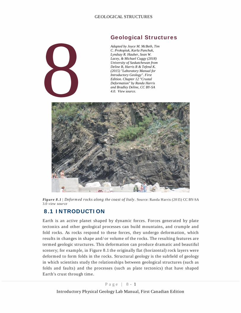
Figure 8.1 | Deformed rocks along the coast of Italy. Source: Randa Harris (2015) CC BY-SA 3.0 view source

8.1 INTRODUCTION Earth is an active planet shaped by dynamic forces. Forces generated by plate tectonics and other geological processes can build mountains, and crumple and fold rocks. As rocks respond to these forces, they undergo deformation, which results in changes in shape and/or volume of the rocks. The resulting features are termed geologic structures. This deformation can produce dramatic and beautiful scenery; for example, in Figure 8.1 the originally flat (horizontal) rock layers were deformed to form folds in the rocks. Structural geology is the subfield of geology in which scientists study the relationships between geological structures (such as folds and faults) and the processes (such as plate tectonics) that have shaped Earth's crust through time.

8

https://ung.edu/university-press/books/laboratory-manual-for-introductory-geology.php


P a g e | 8 - 2


Why is it important to study structures and deformation within the crust? These studies can provide us with a record of the geologic history in a region, and also give us clues to the broader geological processes happening globally through time. This information can be critical when searching for valuable mineral resources. The correct interpretation of features created during deformation helps geologists find oil and valuable metal ores in the petroleum and mining industry, respectively. It is also essential for engineers to understand the behavior of deformed rocks to create and maintain safely engineered structures (e.g., in open and underground mines, and for roads).

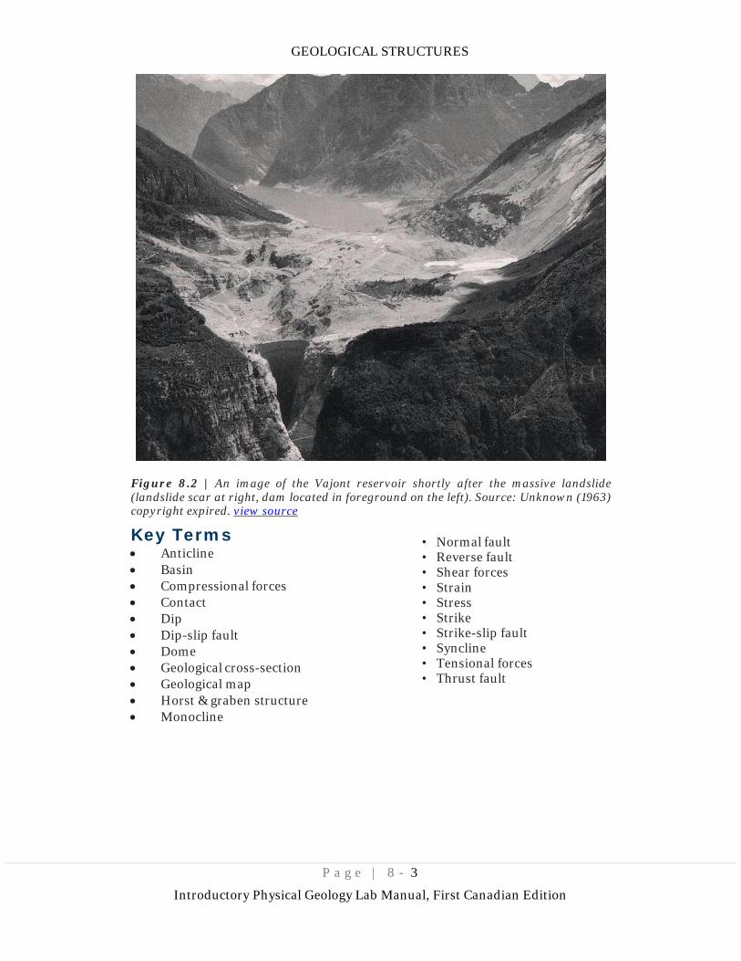
When engineers do not adequately consider geology in their planning - for example by excluding consideration of geological structures - disaster can strike. An example of this is the disaster that occurred at the Vajont Dam, Monte Toc, Italy in the early 1960s. The location was a poor choice for a dam: the valley was steep and narrow with undercut riverbanks at the base and the area surrounding the dam was prone to large landslides due to solution cavities in the limestone canyon walls which could fill with water and interbedded claystones that generated zones of structural weakness in the rocks. Thorough geological tests were not performed prior to construction. Shifting and fracturing of rock that occurred during the filling of the reservoir and faster downhill movement of surface geological deposits were warning signs that went unheeded. In 1963, a massive landslide in the area displaced much of the water in the dam, causing it to override the top of the dam and flood the many villages downstream, resulting in the deaths of almost 2,000 people (Figure 8.2).

There are two parts to this chapter overviewing geological structures:

Part I - strike, dip, and structural cross-sections: overview of the methods geologists use to describe geological structures, including strike and dip measurements, representations of geological structures on maps, how to construct geological cross-sections and measure the thicknesses of geologic units; and

Part II - folds, faults, and unconformities: overview of how to interpret and draw more complex geological structures on geological maps and cross-sections.

8.1.1 Learning Outcomes After completing this chapter, you should be able to: • Demonstrate an understanding of the concepts of strike and dip • Use block diagrams to display geologic features • Interpret a geologic map • Create a geologic cross-section from a geologic map • Understand the types of stress that rocks undergo, and their responses to

stress • Recognize different types of folds and faults, and the forces that create them


P a g e | 8 - 3


Figure 8.2 | An image of the Vajont reservoir shortly after the massive landslide (landslide scar at right, dam located in foreground on the left). Source: Unknown (1963) copyright expired. view source

Key Terms • Anticline • Basin • Compressional forces • Contact • Dip • Dip-slip fault • Dome • Geological cross-section • Geological map • Horst & graben structure • Monocline

• Normal fault • Reverse fault • Shear forces • Strain • Stress • Strike • Strike-slip fault • Syncline • Tensional forces • Thrust fault

https://commons.wikimedia.org/wiki/File:Disastro_Vajont.jpg


P a g e | 8 - 4


Overview of Geological Structures Part I: Strike, Dip, and Structural Cross-Sections

In Part I of geological structures, students will learn how to interpret strike and dip information from a geological map, prepare a geological cross-section from a plan-view geological map, and measure the thicknesses of geological units.

8.2 STRIKE AND DIP To learn many of the concepts associated with structural geology, it is useful to look at block diagrams and block models. Block diagrams are images based on three-dimensional (3-D) block models, which are blocks of wood or paper with geological structures marked on them. Block models and block diagrams assist in visualizing how 3-D geological structures in the real world can be represented in two dimensions on a map or in a geological cross-section.

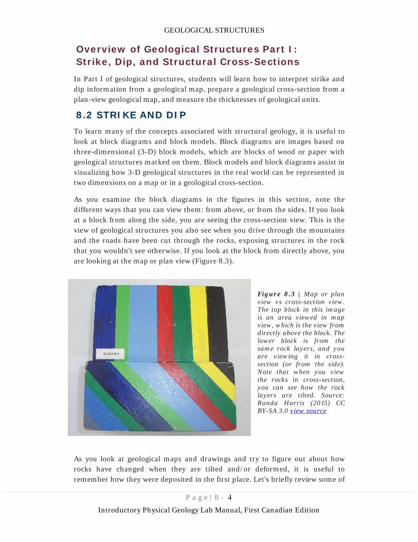
As you examine the block diagrams in the figures in this section, note the different ways that you can view them: from above, or from the sides. If you look at a block from along the side, you are seeing the cross-section view. This is the view of geological structures you also see when you drive through the mountains and the roads have been cut through the rocks, exposing structures in the rock that you wouldn't see otherwise. If you look at the block from directly above, you are looking at the map or plan view (Figure 8.3).

Figure 8.3 | Map or plan view vs cross-section view. The top block in this image is an area viewed in map view, which is the view from directly above the block. The lower block is from the same rock layers, and you are viewing it in cross-section (or from the side). Note that when you view the rocks in cross-section, you can see how the rock layers are tilted. Source: Randa Harris (2015) CC BY-SA 3.0 view source

As you look at geological maps and drawings and try to figure out about how rocks have changed when they are tilted and/or deformed, it is useful to remember how they were deposited in the first place. Let's briefly review some of



P a g e | 8 - 5


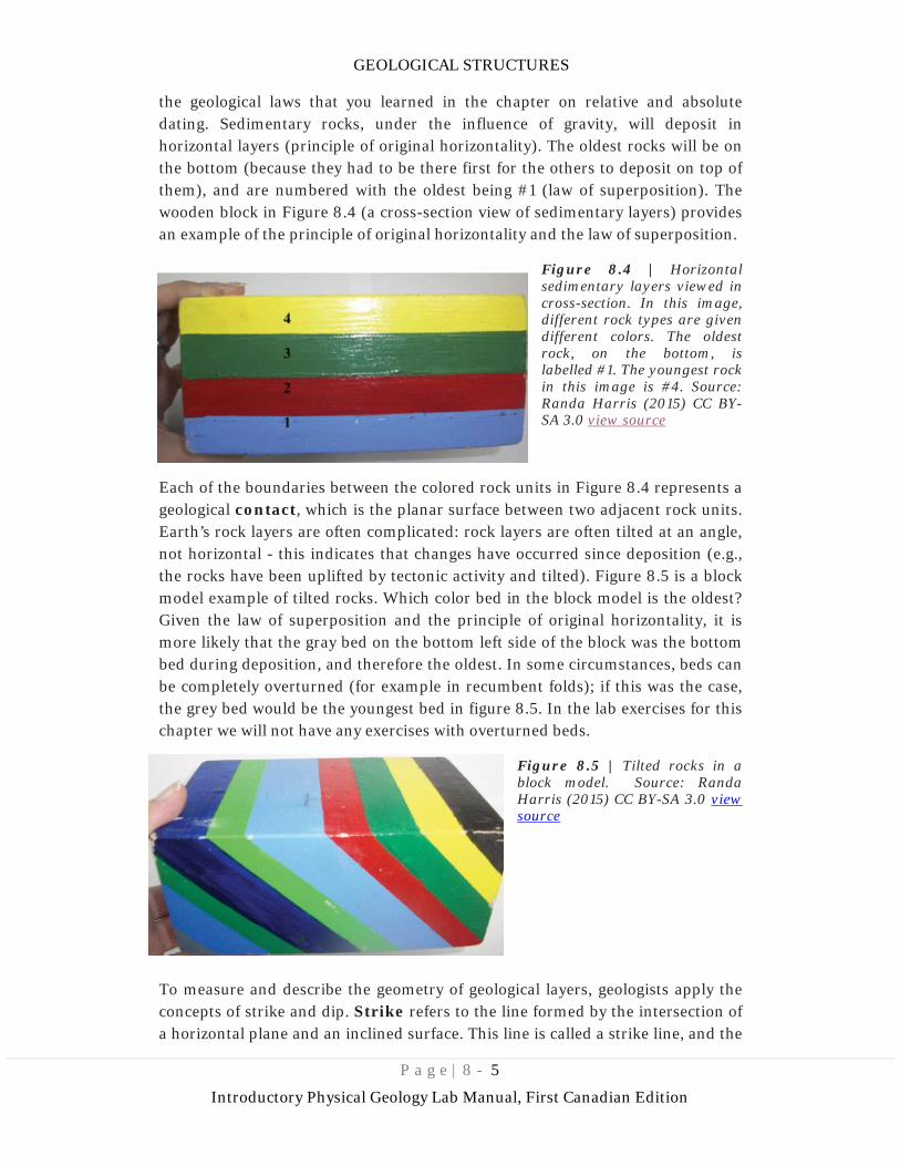
the geological laws that you learned in the chapter on relative and absolute dating. Sedimentary rocks, under the influence of gravity, will deposit in horizontal layers (principle of original horizontality). The oldest rocks will be on the bottom (because they had to be there first for the others to deposit on top of them), and are numbered with the oldest being #1 (law of superposition). The wooden block in Figure 8.4 (a cross-section view of sedimentary layers) provides an example of the principle of original horizontality and the law of superposition.

Figure 8.4 | Horizontal sedimentary layers viewed in cross-section. In this image, different rock types are given different colors. The oldest rock, on the bottom, is labelled #1. The youngest rock in this image is #4. Source: Randa Harris (2015) CC BY-SA 3.0 view source

Each of the boundaries between the colored rock units in Figure 8.4 represents a geological contact, which is the planar surface between two adjacent rock units. Earth’s rock layers are often complicated: rock layers are often tilted at an angle, not horizontal - this indicates that changes have occurred since deposition (e.g., the rocks have been uplifted by tectonic activity and tilted). Figure 8.5 is a block model example of tilted rocks. Which color bed in the block model is the oldest? Given the law of superposition and the principle of original horizontality, it is more likely that the gray bed on the bottom left side of the block was the bottom bed during deposition, and therefore the oldest. In some circumstances, beds can be completely overturned (for example in recumbent folds); if this was the case, the grey bed would be the youngest bed in figure 8.5. In the lab exercises for this chapter we will not have any exercises with overturned beds.

Figure 8.5 | Tilted rocks in a block model. Source: Randa Harris (2015) CC BY-SA 3.0 view source

To measure and describe the geometry of geological layers, geologists apply the concepts of strike and dip. Strike refers to the line formed by the intersection of a horizontal plane and an inclined surface. This line is called a strike line, and the





P a g e | 8 - 6


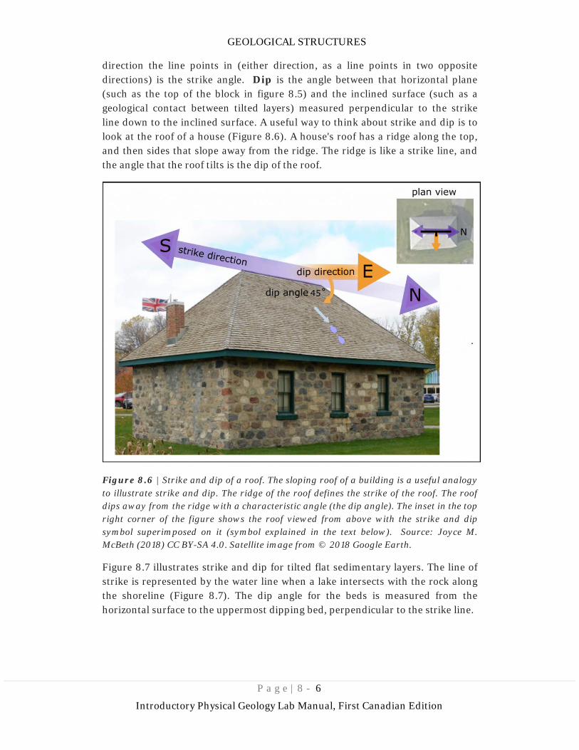
direction the line points in (either direction, as a line points in two opposite directions) is the strike angle. Dip is the angle between that horizontal plane (such as the top of the block in figure 8.5) and the inclined surface (such as a geological contact between tilted layers) measured perpendicular to the strike line down to the inclined surface. A useful way to think about strike and dip is to look at the roof of a house (Figure 8.6). A house's roof has a ridge along the top, and then sides that slope away from the ridge. The ridge is like a strike line, and the angle that the roof tilts is the dip of the roof.

Figure 8.6 | Strike and dip of a roof. The sloping roof of a building is a useful analogy to illustrate strike and dip. The ridge of the roof defines the strike of the roof. The roof dips away from the ridge with a characteristic angle (the dip angle). The inset in the top right corner of the figure shows the roof viewed from above with the strike and dip symbol superimposed on it (symbol explained in the text below). Source: Joyce M. McBeth (2018) CC BY-SA 4.0. Satellite image from © 2018 Google Earth.

Figure 8.7 illustrates strike and dip for tilted flat sedimentary layers. The line of strike is represented by the water line when a lake intersects with the rock along the shoreline (Figure 8.7). The dip angle for the beds is measured from the horizontal surface to the uppermost dipping bed, perpendicular to the strike line.

https://openpress.usask.ca/geolmanual/chapter/overview-of-strike-dip-and-structural-cross-sections/strikediphouse/


P a g e | 8 - 7


Figure 8.7 | Strike and dip for tilted sedimentary beds. Water provides a horizontal surface. The strike and dip symbol is a T with the long horizontal bar representing the strike direction, and the small tick mark indicating the dip direction. The dip angle is written next to the tick mark. Source: Karla Panchuk (2018) CC BY 4.0. Modified after Steven Earle (2015) CC BY 4.0 view source

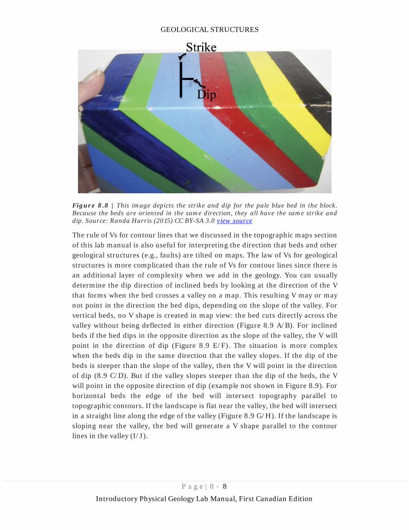
Now, let’s apply this concept to the block of dipping beds in Figure 8.5. To find a strike line, find where a contact intersects the horizontal surface. Each dipping contact intersects the horizontal surface in a horizontal line, so there are many strike lines to choose from. To determine dip, pretend that there is a drop of water between one bed and the next, for example, along the intersection of the pale blue bed and the red bed. In which direction would the water roll if it followed that contact? That is the direction of dip — here, it is towards the right side of the figure. Note that the dip symbol (shorter line) should be drawn perpendicular to the strike symbol, whatever the angle of dip (Figure 8.8).

https://openpress.usask.ca/physicalgeology/chapter/13-5-measuring-geological-structures/


P a g e | 8 - 8


Figure 8.8 | This image depicts the strike and dip for the pale blue bed in the block. Because the beds are oriented in the same direction, they all have the same strike and dip. Source: Randa Harris (2015) CC BY-SA 3.0 view source

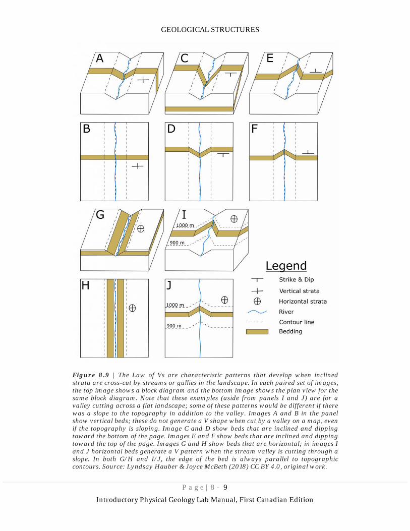
The rule of Vs for contour lines that we discussed in the topographic maps section of this lab manual is also useful for interpreting the direction that beds and other geological structures (e.g., faults) are tilted on maps. The law of Vs for geological structures is more complicated than the rule of Vs for contour lines since there is an additional layer of complexity when we add in the geology. You can usually determine the dip direction of inclined beds by looking at the direction of the V that forms when the bed crosses a valley on a map. This resulting V may or may not point in the direction the bed dips, depending on the slope of the valley. For vertical beds, no V shape is created in map view: the bed cuts directly across the valley without being deflected in either direction (Figure 8.9 A/B). For inclined beds if the bed dips in the opposite direction as the slope of the valley, the V will point in the direction of dip (Figure 8.9 E/F). The situation is more complex when the beds dip in the same direction that the valley slopes. If the dip of the beds is steeper than the slope of the valley, then the V will point in the direction of dip (8.9 C/D). But if the valley slopes steeper than the dip of the beds, the V will point in the opposite direction of dip (example not shown in Figure 8.9). For horizontal beds the edge of the bed will intersect topography parallel to topographic contours. If the landscape is flat near the valley, the bed will intersect in a straight line along the edge of the valley (Figure 8.9 G/H). If the landscape is sloping near the valley, the bed will generate a V shape parallel to the contour lines in the valley (I/J).



P a g e | 8 - 9


Figure 8.9 | The Law of Vs are characteristic patterns that develop when inclined strata are cross-cut by streams or gullies in the landscape. In each paired set of images, the top image shows a block diagram and the bottom image shows the plan view for the same block diagram. Note that these examples (aside from panels I and J) are for a valley cutting across a flat landscape; some of these patterns would be different if there was a slope to the topography in addition to the valley. Images A and B in the panel show vertical beds; these do not generate a V shape when cut by a valley on a map, even if the topography is sloping. Image C and D show beds that are inclined and dipping toward the bottom of the page. Images E and F show beds that are inclined and dipping toward the top of the page. Images G and H show beds that are horizontal; in images I and J horizontal beds generate a V pattern when the stream valley is cutting through a slope. In both G/H and I/J, the edge of the bed is always parallel to topographic contours. Source: Lyndsay Hauber & Joyce McBeth (2018) CC BY 4.0, original work.

https://openpress.usask.ca/geolmanual/chapter/overview-of-strike-dip-and-structural-cross-sections/figure_8-8-2/


P a g e | 8 - 10


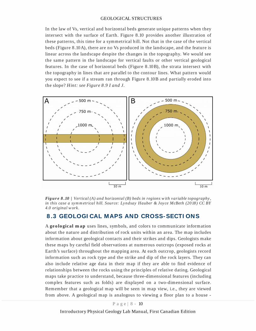
In the law of Vs, vertical and horizontal beds generate unique patterns when they intersect with the surface of Earth. Figure 8.10 provides another illustration of these patterns, this time for a symmetrical hill. Not that in the case of the vertical beds (Figure 8.10A), there are no Vs produced in the landscape, and the feature is linear across the landscape despite the changes in the topography. We would see the same pattern in the landscape for vertical faults or other vertical geological features. In the case of horizontal beds (Figure 8.10B), the strata intersect with the topography in lines that are parallel to the contour lines. What pattern would you expect to see if a stream ran through Figure 8.10B and partially eroded into the slope? Hint: see Figure 8.9 I and J.

Figure 8.10 | Vertical (A) and horizontal (B) beds in regions with variable topography, in this case a symmetrical hill. Source: Lyndsay Hauber & Joyce McBeth (2018) CC BY 4.0 original work.

8.3 GEOLOGICAL MAPS AND CROSS-SECTIONS A geological map uses lines, symbols, and colors to communicate information about the nature and distribution of rock units within an area. The map includes information about geological contacts and their strikes and dips. Geologists make these maps by careful field observations at numerous outcrops (exposed rocks at Earth’s surface) throughout the mapping area. At each outcrop, geologists record information such as rock type and the strike and dip of the rock layers. They can also include relative age data in their map if they are able to find evidence of relationships between the rocks using the principles of relative dating. Geological maps take practice to understand, because three-dimensional features (including complex features such as folds) are displayed on a two-dimensional surface. Remember that a geological map will be seen in map view, i.e., they are viewed from above. A geological map is analogous to viewing a floor plan to a house -


P a g e | 8 - 11


there are many things you can represent in plan view (e.g., doors, appliances, stairs) that will help you visualize what the interior will look like if you were to visit the house in real life.

Geologists use information about rocks that are exposed to visualize how the unseen rocks beneath the surface are oriented. This allows geologists to prepare their best interpretation of the cross-sectional view of the geology below the surface, similar to what we observed in the blocks above.

A geological cross-section shows geologic features from the side view (the side views of the block diagrams in Figures 8.3-8.5 are cross-sections). They are similar to the topographic profiles that you created in the topographic maps chapter, but they also show the rock types and geologic structures present beneath Earth’s surface.

There are four things to include on every geological cross-section: a legend, the orientation of the line the cross-section represents on the map, a title, and a scale (e.g., Figure 8.11C). To help us remember, we abbreviate these four key parts with the acronym L.O.T.S.

Legend – the legend is a key to the patterns used to identify each unit on the cross-section. The units are ordered from oldest formation at the bottom of the legend to youngest unit at the top of the legend.

Orientation – the orientation of the cross-section is the direction that the cross-section line makes on Earth (the “strike” direction of the cross-section line on the geological map). You can indicate the orientation by writing the corresponding direction at each end of the cross-section (e.g., west and east on Figure 8.11C).

Title – a descriptive title for the cross-section. You can include the letters used to identify the line on the original geological map in the title (e.g., Cross-Section along Line X-Y in Figure 8.11C).

Scale – include a ratio scale and/or a bar scale to show the scale of the cross-section. The vertical and horizonal scales should be the same, so you only need to include one scale on the cross-section.


P a g e | 8 - 12


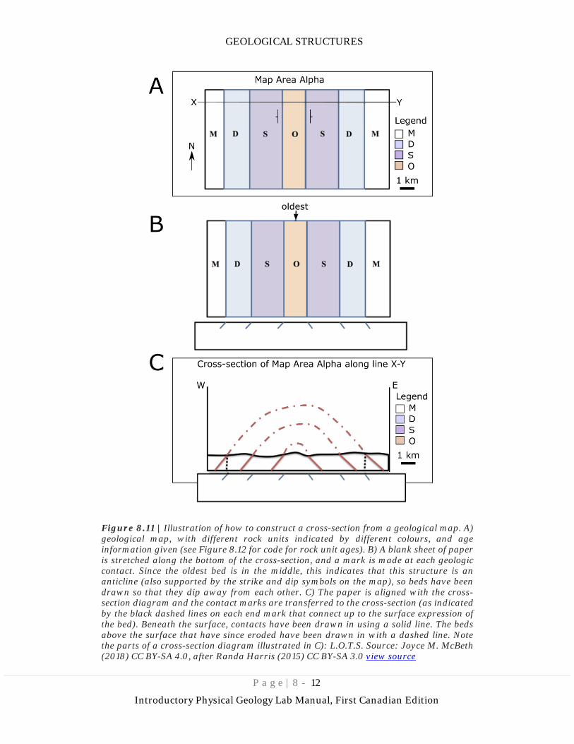
Figure 8.11 | Illustration of how to construct a cross-section from a geological map. A) geological map, with different rock units indicated by different colours, and age information given (see Figure 8.12 for code for rock unit ages). B) A blank sheet of paper is stretched along the bottom of the cross-section, and a mark is made at each geologic contact. Since the oldest bed is in the middle, this indicates that this structure is an anticline (also supported by the strike and dip symbols on the map), so beds have been drawn so that they dip away from each other. C) The paper is aligned with the cross-section diagram and the contact marks are transferred to the cross-section (as indicated by the black dashed lines on each end mark that connect up to the surface expression of the bed). Beneath the surface, contacts have been drawn in using a solid line. The beds above the surface that have since eroded have been drawn in with a dashed line. Note the parts of a cross-section diagram illustrated in C): L.O.T.S. Source: Joyce M. McBeth (2018) CC BY-SA 4.0, after Randa Harris (2015) CC BY-SA 3.0 view source



P a g e | 8 - 13


Figure 8.11 provides an example of a simple geological cross-section. To construct a geological cross-section, follow these steps:

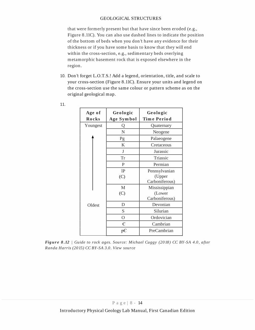
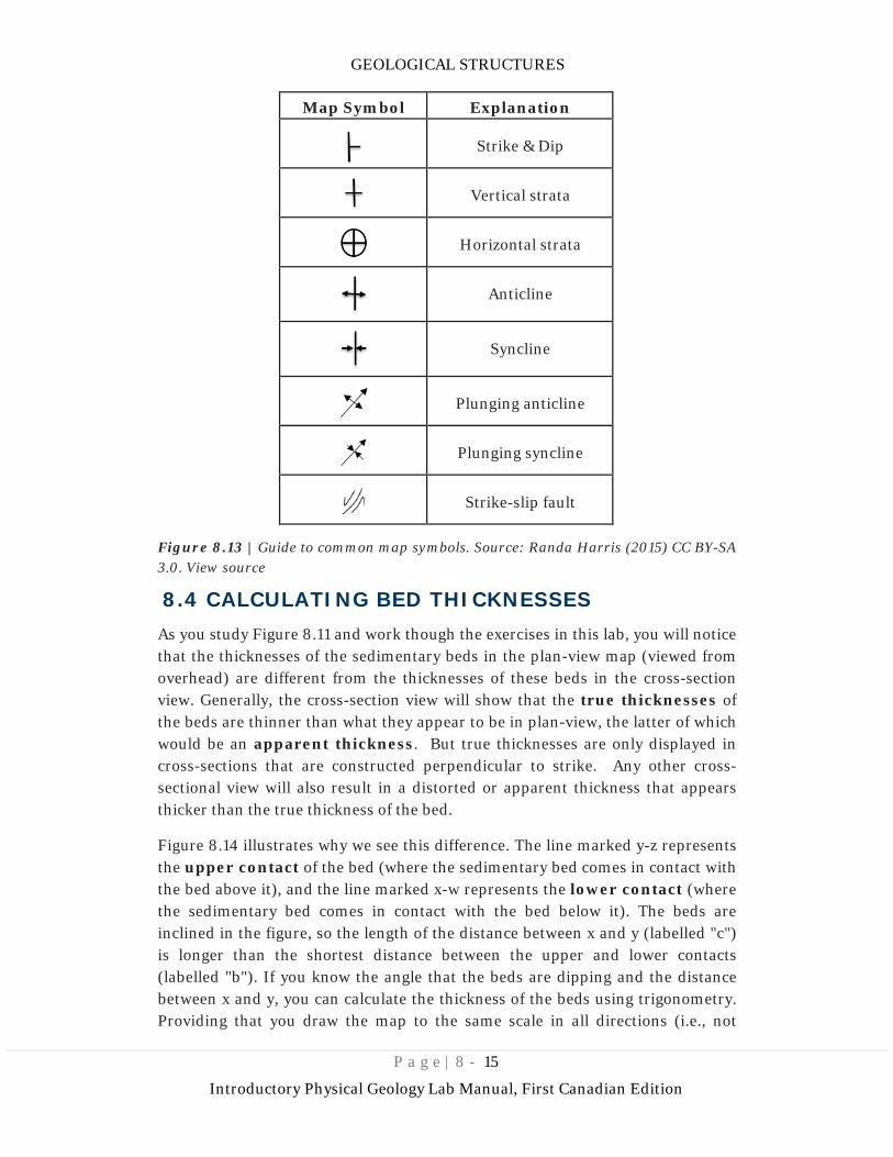
1. Carefully look at the geological map that you are using to construct your cross-section (e.g., Figure 8.11A). Pay close attention to any strike and dip symbols, geological contacts, and ages of the rock types (Figures 8.12 and 8.13 have examples of rock age abbreviations and common structural symbols used on geological maps).

2. Identify the position on the map designated for the cross-section. The line will be indicated by an actual line, or with positions labelled with letters on the edges of the map, e.g., “X” and “Y”.

3. Take a clean sheet of paper, and line it up along the line on the plan view map (Figure 8.11B). At each geological contact, make a mark on the edge of the paper.

4. Using any strike and dip symbols on the map, add the dip onto the marks on your piece of paper, showing the direction the rocks are dipping, and note the angle of dip for each position.

5. If strike and dip symbols are not provided but based on the Law of Vs or the ages of the beds you are able to determine that there are dipping or vertical structures present, include these as corresponding marks on your paper. Use your best interpretation of the dip direction if dips are not given on the geological map.

6. Transfer the marks from your paper to the bottom of the cross-section diagram provided (Figure 8.11C). You can prepare your own cross-section diagram based on the example in the exercises section of this chapter. The x-axis of the diagram will be the distance along the line on the map, and the z-axis will be the elevation of the rocks (usually measured relative to sea level or another benchmark).

7. Draw the topography on the cross-section (just as you did in the exercises in the topographic maps chapter). Note that in the example in figure 8.11 the map area is flat.

8. Transfer the marks from along the edge of your piece of paper to the points along the line where they intersect with the topography. These are the points where the geological structures are exposed at the surface.

9. Sketch the structures into your cross-section, starting at the points where the structures meet the topographic surface. Pay careful attention to dip angles (if they were provided). Structures may be drawn in with a dotted line above Earth’s surface to indicate rocks


P a g e | 8 - 14


that were formerly present but that have since been eroded (e.g., Figure 8.11C). You can also use dashed lines to indicate the position of the bottom of beds when you don’t have any evidence for their thickness or if you have some basis to know that they will end within the cross-section, e.g., sedimentary beds overlying metamorphic basement rock that is exposed elsewhere in the region.

10. Don’t forget L.O.T.S.! Add a legend, orientation, title, and scale to your cross-section (Figure 8.11C). Ensure your units and legend on the cross-section use the same colour or pattern scheme as on the original geological map.

11.

Age of Rocks

Geologic Age Symbol

Geologic Time Period

Youngest

Oldest

Q Quaternary N Neogene

Pg Palaeogene K Cretaceous J Jurassic

Tr Triassic P Permian lP

(C) Pennsylvanian

(Upper Carboniferous)

M (C)

Mississippian (Lower

Carboniferous) D Devonian S Silurian O Ordovician Є Cambrian pЄ PreCambrian

Figure 8.12 | Guide to rock ages. Source: Michael Cuggy (2018) CC BY-SA 4.0, after Randa Harris (2015) CC BY-SA 3.0. View source


P a g e | 8 - 15


Map Symbol Explanation

Strike & Dip

Vertical strata

Horizontal strata

Anticline

Syncline

Plunging anticline

Plunging syncline

Strike-slip fault

Figure 8.13 | Guide to common map symbols. Source: Randa Harris (2015) CC BY-SA 3.0. View source

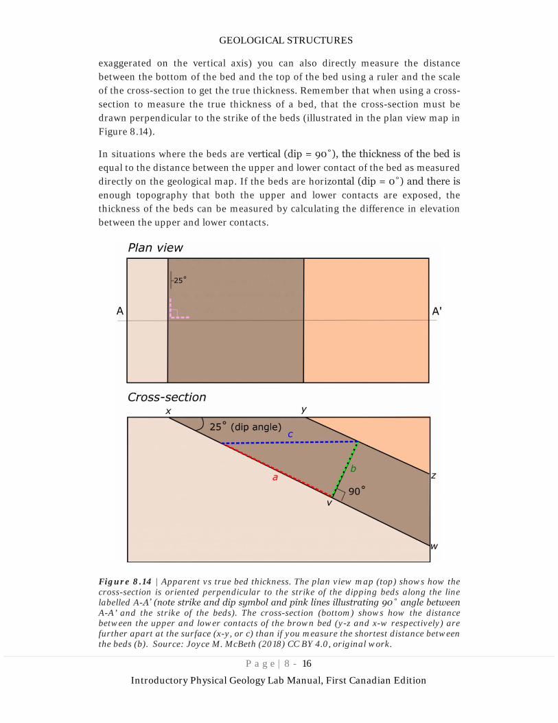
8.4 CALCULATING BED THICKNESSES As you study Figure 8.11 and work though the exercises in this lab, you will notice that the thicknesses of the sedimentary beds in the plan-view map (viewed from overhead) are different from the thicknesses of these beds in the cross-section view. Generally, the cross-section view will show that the true thicknesses of the beds are thinner than what they appear to be in plan-view, the latter of which would be an apparent thickness. But true thicknesses are only displayed in cross-sections that are constructed perpendicular to strike. Any other cross-sectional view will also result in a distorted or apparent thickness that appears thicker than the true thickness of the bed.

Figure 8.14 illustrates why we see this difference. The line marked y-z represents the upper contact of the bed (where the sedimentary bed comes in contact with the bed above it), and the line marked x-w represents the lower contact (where the sedimentary bed comes in contact with the bed below it). The beds are inclined in the figure, so the length of the distance between x and y (labelled "c") is longer than the shortest distance between the upper and lower contacts (labelled "b"). If you know the angle that the beds are dipping and the distance between x and y, you can calculate the thickness of the beds using trigonometry. Providing that you draw the map to the same scale in all directions (i.e., not


P a g e | 8 - 16


exaggerated on the vertical axis) you can also directly measure the distance between the bottom of the bed and the top of the bed using a ruler and the scale of the cross-section to get the true thickness. Remember that when using a cross-section to measure the true thickness of a bed, that the cross-section must be drawn perpendicular to the strike of the beds (illustrated in the plan view map in Figure 8.14).

In situations where the beds are vertical (dip = 90˚), the thickness of the bed is equal to the distance between the upper and lower contact of the bed as measured directly on the geological map. If the beds are horizontal (dip = 0˚) and there is enough topography that both the upper and lower contacts are exposed, the thickness of the beds can be measured by calculating the difference in elevation between the upper and lower contacts.

Figure 8.14 | Apparent vs true bed thickness. The plan view map (top) shows how the cross-section is oriented perpendicular to the strike of the dipping beds along the line labelled A-A’ (note strike and dip symbol and pink lines illustrating 90˚ angle between A-A’ and the strike of the beds). The cross-section (bottom) shows how the distance between the upper and lower contacts of the brown bed (y-z and x-w respectively) are further apart at the surface (x-y, or c) than if you measure the shortest distance between the beds (b). Source: Joyce M. McBeth (2018) CC BY 4.0, original work.


P a g e | 8 - 17


Overview of Geological Structures Part II: Stress and Strain, Folds, Faults, and Unconformities

In Part II of geological structures, students will learn how stress and strain create more complex geological structures, and also how to interpret geological maps that display folded and faulted structures, as well as unconformities.

8.5 STRESS AND STRAIN

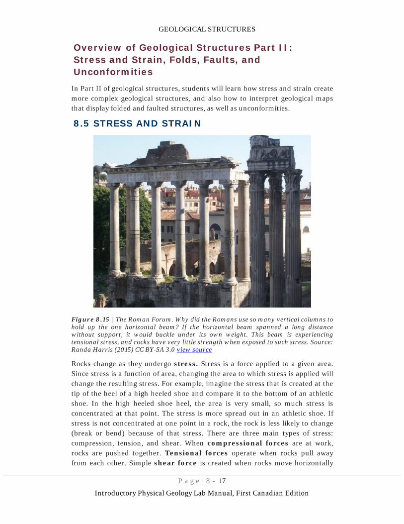
Figure 8.15 | The Roman Forum. Why did the Romans use so many vertical columns to hold up the one horizontal beam? If the horizontal beam spanned a long distance without support, it would buckle under its own weight. This beam is experiencing tensional stress, and rocks have very little strength when exposed to such stress. Source: Randa Harris (2015) CC BY-SA 3.0 view source

Rocks change as they undergo stress. Stress is a force applied to a given area. Since stress is a function of area, changing the area to which stress is applied will change the resulting stress. For example, imagine the stress that is created at the tip of the heel of a high heeled shoe and compare it to the bottom of an athletic shoe. In the high heeled shoe heel, the area is very small, so much stress is concentrated at that point. The stress is more spread out in an athletic shoe. If stress is not concentrated at one point in a rock, the rock is less likely to change (break or bend) because of that stress. There are three main types of stress: compression, tension, and shear. When compressional forces are at work, rocks are pushed together. Tensional forces operate when rocks pull away from each other. Simple shear force is created when rocks move horizontally



P a g e | 8 - 18


past each other in opposite directions. Rocks can withstand much more compressional stress than tensional stress (e.g., Figure 8.15).

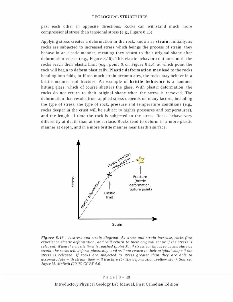
Applying stress creates a deformation in the rock, known as strain. Initially, as rocks are subjected to increased stress which beings the process of strain, they behave in an elastic manner, meaning they return to their original shape after deformation ceases (e.g., Figure 8.16). This elastic behavior continues until the rocks reach their elastic limit (e.g., point X on Figure 8.16), at which point the rock will begin to deform plastically. Plastic deformation may lead to the rocks bending into folds, or if too much strain accumulates, the rocks may behave in a brittle manner and fracture. An example of brittle behavior is a hammer hitting glass, which of course shatters the glass. With plastic deformation, the rocks do not return to their original shape when the stress is removed. The deformation that results from applied stress depends on many factors, including the type of stress, the type of rock, pressure and temperature conditions (e.g., rocks deeper in the crust will be subject to higher pressures and temperatures), and the length of time the rock is subjected to the stress. Rocks behave very differently at depth than at the surface. Rocks tend to deform in a more plastic manner at depth, and in a more brittle manner near Earth’s surface.

Figure 8.16 | A stress and strain diagram. As stress and strain increase, rocks first experience elastic deformation, and will return to their original shape if the stress is released. When the elastic limit is reached (point X), if stress continues to accumulate as strain, the rocks will deform plastically, and will not return to their original shape if the stress is released. If rocks are subjected to stress greater than they are able to accommodate with strain, they will fracture (brittle deformation, yellow star). Source: Joyce M. McBeth (2018) CC BY 4.0.


P a g e | 8 - 19


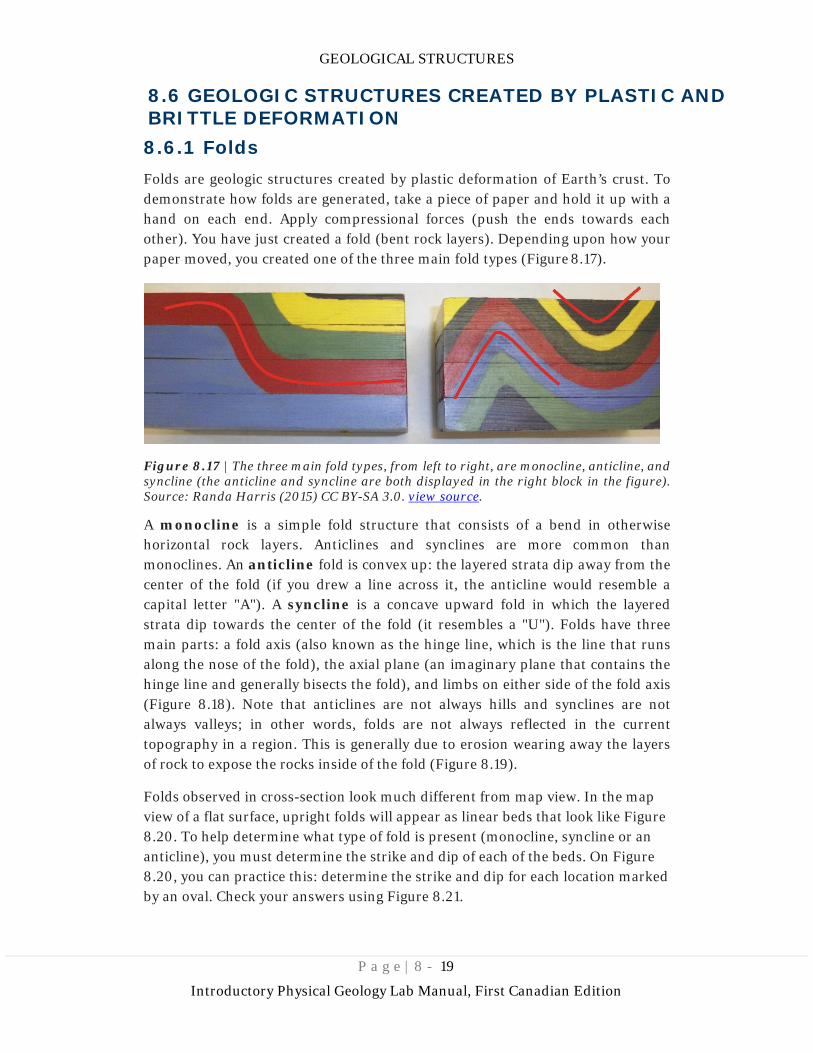
8.6 GEOLOGIC STRUCTURES CREATED BY PLASTIC AND BRITTLE DEFORMATION 8.6.1 Folds Folds are geologic structures created by plastic deformation of Earth’s crust. To demonstrate how folds are generated, take a piece of paper and hold it up with a hand on each end. Apply compressional forces (push the ends towards each other). You have just created a fold (bent rock layers). Depending upon how your paper moved, you created one of the three main fold types (Figure 8.17).

Figure 8.17 | The three main fold types, from left to right, are monocline, anticline, and syncline (the anticline and syncline are both displayed in the right block in the figure). Source: Randa Harris (2015) CC BY-SA 3.0. view source.

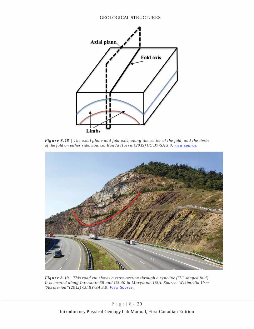
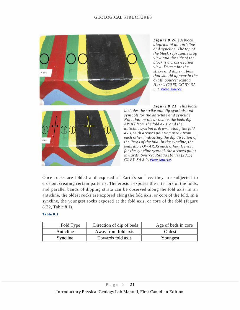
A monocline is a simple fold structure that consists of a bend in otherwise horizontal rock layers. Anticlines and synclines are more common than monoclines. An anticline fold is convex up: the layered strata dip away from the center of the fold (if you drew a line across it, the anticline would resemble a capital letter "A"). A syncline is a concave upward fold in which the layered strata dip towards the center of the fold (it resembles a "U"). Folds have three main parts: a fold axis (also known as the hinge line, which is the line that runs along the nose of the fold), the axial plane (an imaginary plane that contains the hinge line and generally bisects the fold), and limbs on either side of the fold axis (Figure 8.18). Note that anticlines are not always hills and synclines are not always valleys; in other words, folds are not always reflected in the current topography in a region. This is generally due to erosion wearing away the layers of rock to expose the rocks inside of the fold (Figure 8.19).

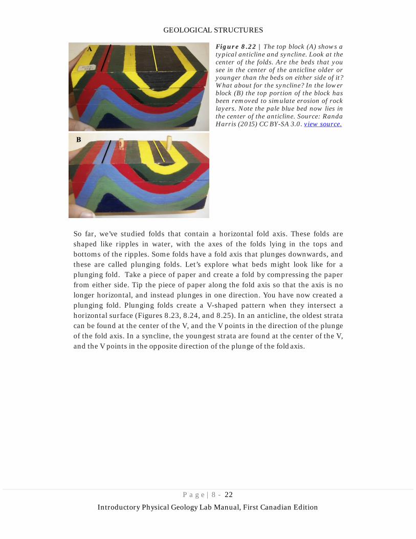
Folds observed in cross-section look much different from map view. In the map view of a flat surface, upright folds will appear as linear beds that look like Figure 8.20. To help determine what type of fold is present (monocline, syncline or an anticline), you must determine the strike and dip of each of the beds. On Figure 8.20, you can practice this: determine the strike and dip for each location marked by an oval. Check your answers using Figure 8.21.



P a g e | 8 - 20


Figure 8.18 | The axial plane and fold axis, along the center of the fold, and the limbs of the fold on either side. Source: Randa Harris (2015) CC BY-SA 3.0. view source.

Figure 8.19 | This road cut shows a cross-section through a syncline ("U" shaped fold). It is located along Interstate 68 and US 40 in Maryland, USA. Source: Wikimedia User “Acroterion” (2012) CC BY-SA 3.0. View Source.


https://commons.wikimedia.org/wiki/File:Sideling_Hill_cut_MD1.jpg


P a g e | 8 - 21


Figure 8.20 | A block diagram of an anticline and syncline. The top of the block represents map view and the side of the block is a cross-section view. Determine the strike and dip symbols that should appear in the ovals. Source: Randa Harris (2015) CC BY-SA 3.0. view source.

Figure 8.21 | This block includes the strike and dip symbols and symbols for the anticline and syncline. Note that on the anticline, the beds dip AWAY from the fold axis, and the anticline symbol is drawn along the fold axis, with arrows pointing away from each other, indicating the dip direction of the limbs of the fold. In the syncline, the beds dip TOWARDS each other. Hence, for the syncline symbol, the arrows point inwards. Source: Randa Harris (2015) CC BY-SA 3.0. view source.

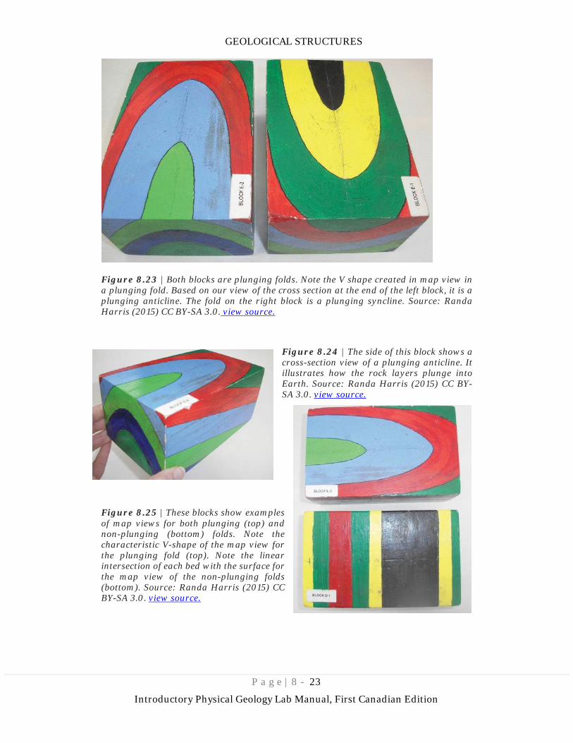
Once rocks are folded and exposed at Earth’s surface, they are subjected to erosion, creating certain patterns. The erosion exposes the interiors of the folds, and parallel bands of dipping strata can be observed along the fold axis. In an anticline, the oldest rocks are exposed along the fold axis, or core of the fold. In a syncline, the youngest rocks exposed at the fold axis, or core of the fold (Figure 8.22, Table 8.1).

Table 8.1

Fold Type Direction of dip of beds Age of beds in core Anticline Away from fold axis Oldest Syncline Towards fold axis Youngest




P a g e | 8 - 22


Figure 8.22 | The top block (A) shows a typical anticline and syncline. Look at the center of the folds. Are the beds that you see in the center of the anticline older or younger than the beds on either side of it? What about for the syncline? In the lower block (B) the top portion of the block has been removed to simulate erosion of rock layers. Note the pale blue bed now lies in the center of the anticline. Source: Randa Harris (2015) CC BY-SA 3.0. view source.

So far, we’ve studied folds that contain a horizontal fold axis. These folds are shaped like ripples in water, with the axes of the folds lying in the tops and bottoms of the ripples. Some folds have a fold axis that plunges downwards, and these are called plunging folds. Let’s explore what beds might look like for a plunging fold. Take a piece of paper and create a fold by compressing the paper from either side. Tip the piece of paper along the fold axis so that the axis is no longer horizontal, and instead plunges in one direction. You have now created a plunging fold. Plunging folds create a V-shaped pattern when they intersect a horizontal surface (Figures 8.23, 8.24, and 8.25). In an anticline, the oldest strata can be found at the center of the V, and the V points in the direction of the plunge of the fold axis. In a syncline, the youngest strata are found at the center of the V, and the V points in the opposite direction of the plunge of the fold axis.



P a g e | 8 - 23


Figure 8.23 | Both blocks are plunging folds. Note the V shape created in map view in a plunging fold. Based on our view of the cross section at the end of the left block, it is a plunging anticline. The fold on the right block is a plunging syncline. Source: Randa Harris (2015) CC BY-SA 3.0. view source.

Figure 8.24 | The side of this block shows a cross-section view of a plunging anticline. It illustrates how the rock layers plunge into Earth. Source: Randa Harris (2015) CC BY-SA 3.0. view source.

Figure 8.25 | These blocks show examples of map views for both plunging (top) and non-plunging (bottom) folds. Note the characteristic V-shape of the map view for the plunging fold (top). Note the linear intersection of each bed with the surface for the map view of the non-plunging folds (bottom). Source: Randa Harris (2015) CC BY-SA 3.0. view source.





P a g e | 8 - 24


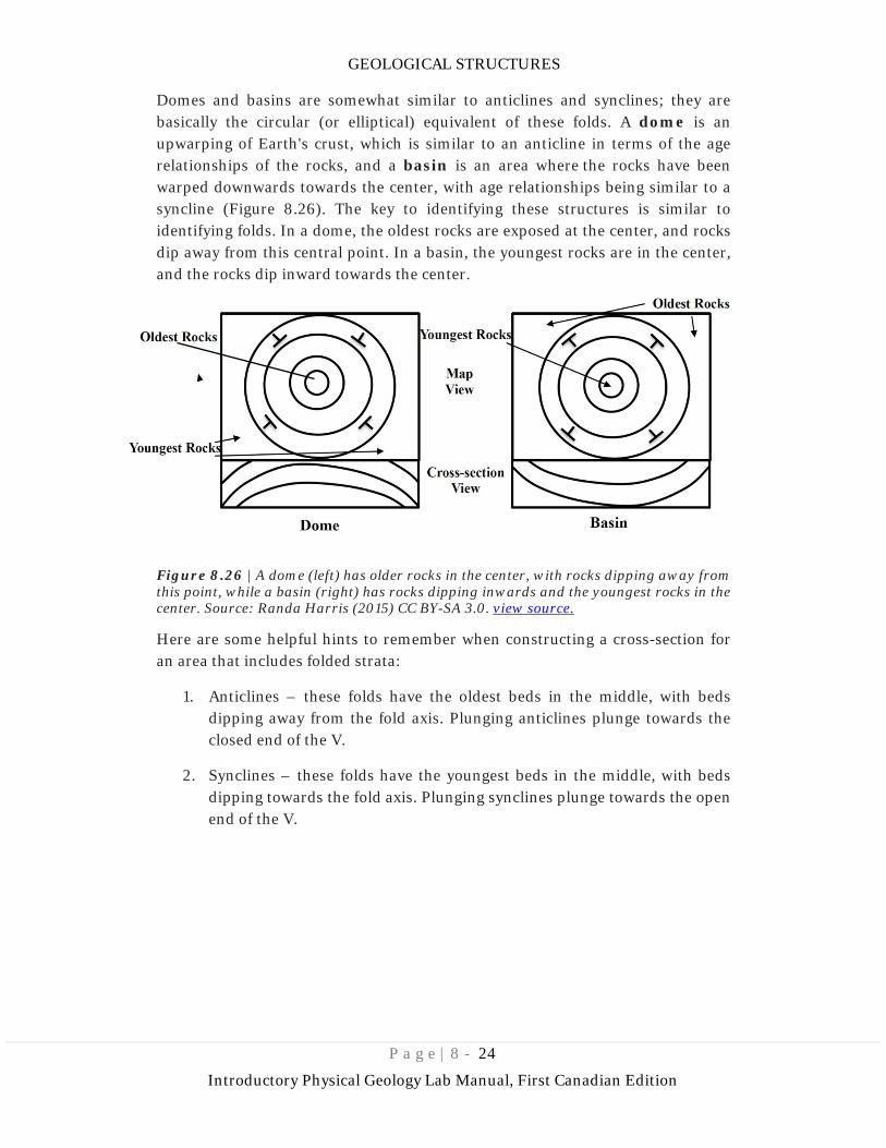
Domes and basins are somewhat similar to anticlines and synclines; they are basically the circular (or elliptical) equivalent of these folds. A dome is an upwarping of Earth's crust, which is similar to an anticline in terms of the age relationships of the rocks, and a basin is an area where the rocks have been warped downwards towards the center, with age relationships being similar to a syncline (Figure 8.26). The key to identifying these structures is similar to identifying folds. In a dome, the oldest rocks are exposed at the center, and rocks dip away from this central point. In a basin, the youngest rocks are in the center, and the rocks dip inward towards the center.

Figure 8.26 | A dome (left) has older rocks in the center, with rocks dipping away from this point, while a basin (right) has rocks dipping inwards and the youngest rocks in the center. Source: Randa Harris (2015) CC BY-SA 3.0. view source.

Here are some helpful hints to remember when constructing a cross-section for an area that includes folded strata:

1. Anticlines – these folds have the oldest beds in the middle, with beds dipping away from the fold axis. Plunging anticlines plunge towards the closed end of the V.

2. Synclines – these folds have the youngest beds in the middle, with beds dipping towards the fold axis. Plunging synclines plunge towards the open end of the V.



P a g e | 8 - 25


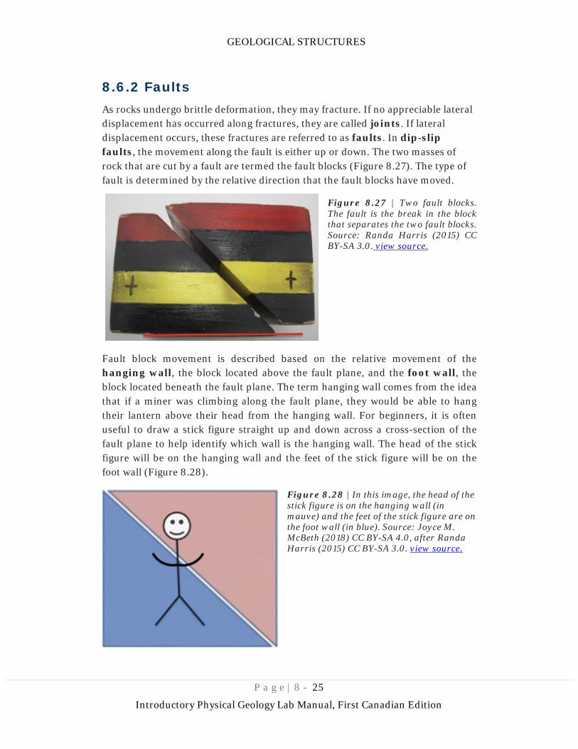
8.6.2 Faults As rocks undergo brittle deformation, they may fracture. If no appreciable lateral displacement has occurred along fractures, they are called joints. If lateral displacement occurs, these fractures are referred to as faults. In dip-slip faults, the movement along the fault is either up or down. The two masses of rock that are cut by a fault are termed the fault blocks (Figure 8.27). The type of fault is determined by the relative direction that the fault blocks have moved.

Figure 8.27 | Two fault blocks. The fault is the break in the block that separates the two fault blocks. Source: Randa Harris (2015) CC BY-SA 3.0. view source.

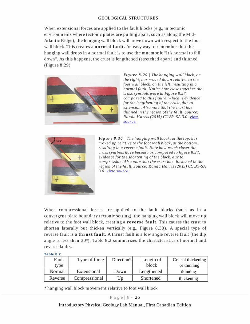
Fault block movement is described based on the relative movement of the hanging wall, the block located above the fault plane, and the foot wall, the block located beneath the fault plane. The term hanging wall comes from the idea that if a miner was climbing along the fault plane, they would be able to hang their lantern above their head from the hanging wall. For beginners, it is often useful to draw a stick figure straight up and down across a cross-section of the fault plane to help identify which wall is the hanging wall. The head of the stick figure will be on the hanging wall and the feet of the stick figure will be on the foot wall (Figure 8.28).

Figure 8.28 | In this image, the head of the stick figure is on the hanging wall (in mauve) and the feet of the stick figure are on the foot wall (in blue). Source: Joyce M. McBeth (2018) CC BY-SA 4.0, after Randa Harris (2015) CC BY-SA 3.0. view source.




P a g e | 8 - 26


When extensional forces are applied to the fault blocks (e.g., in tectonic environments where tectonic plates are pulling apart, such as along the Mid-Atlantic Ridge), the hanging wall block will move down with respect to the foot wall block. This creates a normal fault. An easy way to remember that the hanging wall drops in a normal fault is to use the mnemonic “It’s normal to fall down”. As this happens, the crust is lengthened (stretched apart) and thinned (Figure 8.29).

Figure 8.29 | The hanging wall block, on the right, has moved down relative to the foot wall block, on the left, resulting in a normal fault. Notice how close together the cross symbols were in Figure 8.27, compared to this figure, which is evidence for the lengthening of the crust, due to extension. Also note that the crust has thinned in the region of the fault. Source: Randa Harris (2015) CC BY-SA 3.0. view source.

Figure 8.30 | The hanging wall block, at the top, has moved up relative to the foot wall block, at the bottom, resulting in a reverse fault. Note how much closer the cross symbols have become as compared to figure 8.27, evidence for the shortening of the block, due to compression. Also note that the crust has thickened in the region of the fault. Source: Randa Harris (2015) CC BY-SA 3.0. view source.

When compressional forces are applied to the fault blocks (such as in a convergent plate boundary tectonic setting), the hanging wall block will move up relative to the foot wall block, creating a reverse fault. This causes the crust to shorten laterally but thicken vertically (e.g., Figure 8.30). A special type of reverse fault is a thrust fault. A thrust fault is a low angle reverse fault (the dip angle is less than 30o). Table 8.2 summarizes the characteristics of normal and reverse faults.

Table 8.2

Fault type

Type of force Direction* Length of block

Crustal thickening or thinning

Normal Extensional Down Lengthened thinning Reverse Compressional Up Shortened thickening

* hanging wall block movement relative to foot wall block





P a g e | 8 - 27


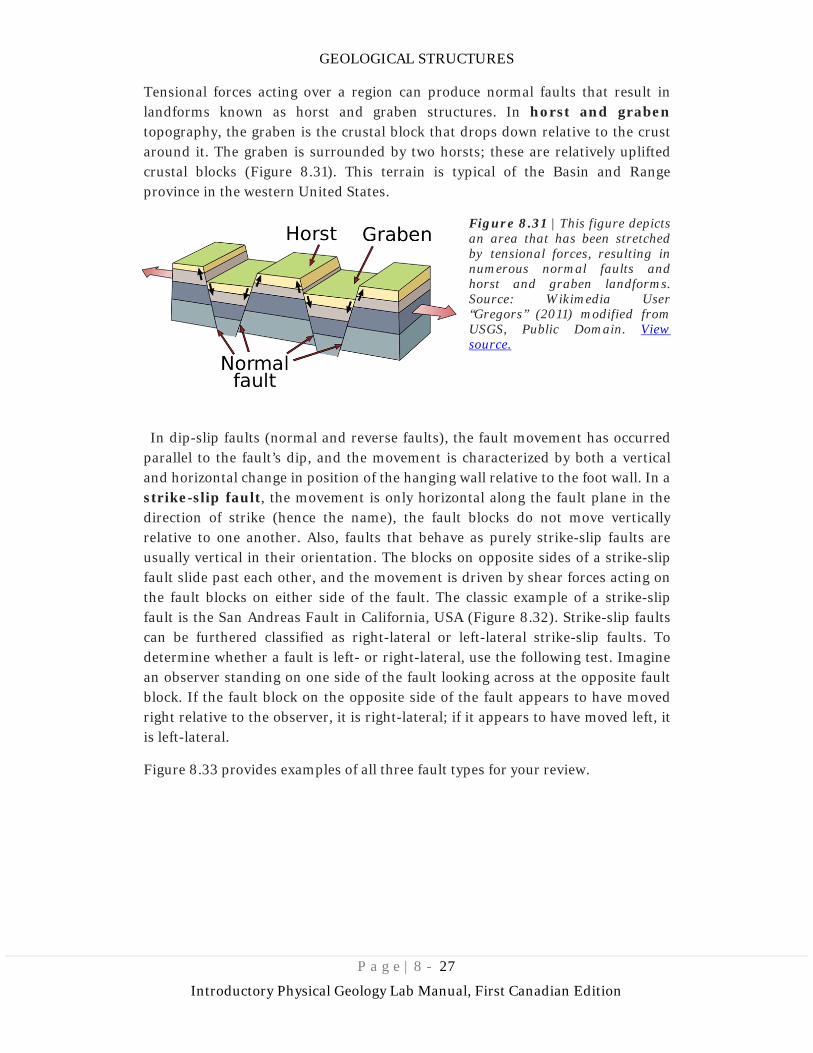
Tensional forces acting over a region can produce normal faults that result in landforms known as horst and graben structures. In horst and graben topography, the graben is the crustal block that drops down relative to the crust around it. The graben is surrounded by two horsts; these are relatively uplifted crustal blocks (Figure 8.31). This terrain is typical of the Basin and Range province in the western United States.

Figure 8.31 | This figure depicts an area that has been stretched by tensional forces, resulting in numerous normal faults and horst and graben landforms. Source: Wikimedia User “Gregors” (2011) modified from USGS, Public Domain. View source.

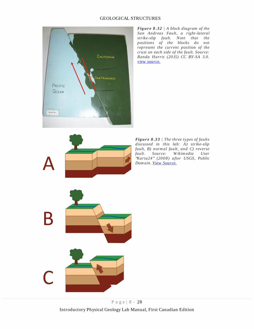
In dip-slip faults (normal and reverse faults), the fault movement has occurred parallel to the fault’s dip, and the movement is characterized by both a vertical and horizontal change in position of the hanging wall relative to the foot wall. In a strike-slip fault, the movement is only horizontal along the fault plane in the direction of strike (hence the name), the fault blocks do not move vertically relative to one another. Also, faults that behave as purely strike-slip faults are usually vertical in their orientation. The blocks on opposite sides of a strike-slip fault slide past each other, and the movement is driven by shear forces acting on the fault blocks on either side of the fault. The classic example of a strike-slip fault is the San Andreas Fault in California, USA (Figure 8.32). Strike-slip faults can be furthered classified as right-lateral or left-lateral strike-slip faults. To determine whether a fault is left- or right-lateral, use the following test. Imagine an observer standing on one side of the fault looking across at the opposite fault block. If the fault block on the opposite side of the fault appears to have moved right relative to the observer, it is right-lateral; if it appears to have moved left, it is left-lateral.

Figure 8.33 provides examples of all three fault types for your review.

https://commons.wikimedia.org/wiki/File:Fault-Horst-Graben.svg

https://commons.wikimedia.org/wiki/File:Fault-Horst-Graben.svg


P a g e | 8 - 28


Figure 8.32 | A block diagram of the San Andreas Fault, a right-lateral strike-slip fault. Note that the positions of the blocks do not represent the current position of the crust on each side of the fault. Source: Randa Harris (2015) CC BY-SA 3.0. view source.

Figure 8.33 | The three types of faults discussed in this lab: A) strike-slip fault, B) normal fault, and C) reverse fault. Source: Wikimedia User “Karta24” (2008) after USGS, Public Domain. View Source.


https://commons.wikimedia.org/wiki/File:Fault_types.svg


P a g e | 8 - 29


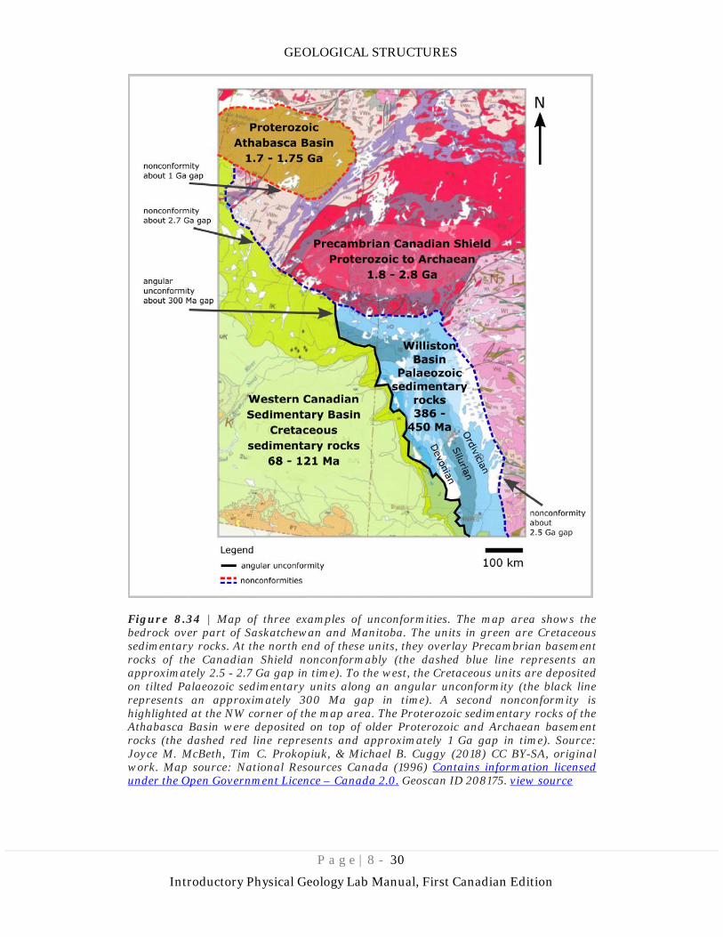
8.7 Unconformities on Geological Maps Unconformities have been discussed in a previous section of this lab manual. Recall the definition of an unconformity: a gap in the geological record where a rock unit is overlain by another rock unit which was deposited substantially later in time. The unconformity is the gap in time between the rocks above and below. Also recall the different types of unconformities: (1) disconformity: a gap in time between parallel sedimentary rocks caused by either erosion or nondeposition during the time period; (2) nonconformity: a gap in time between crystalline (i.e. igneous and metamorphic) basement rock and the sedimentary rocks located immediately upon the basement rock. Nonconformities commonly span vast amounts of time, up to billions of years; and (3) angular unconformity: a gap in time in which a sequence of sedimentary rocks lies upon an older sequence of sedimentary rocks, but these older rocks were tilted so lie in a different orientation than the rocks above.

Identifying unconformities on geological maps can be difficult. Disconformities are almost impossible to locate, unless you are told the ages of the different layers of rocks. In that case, look for the gaps in time and you will locate any disconformities.

Nonconformities can also be tricky, as intrusive contacts can be mistaken for them. But if you locate sedimentary rocks that are located next to large swaths of igneous and metamorphic rocks, you have likely located a nonconformity. Figure 8.34 show examples of nonconformities: the sedimentary rocks of the Athabasca Basin, and the sedimentary rocks of the western Canadian Sedimentary Basin and Williston Basin all rest nonconformably on the metamorphic basement rocks of the Canadian Shield, with gaps in the rock record ranging from 1 – 2.7 Ga.

Angular unconformities can be very simple to locate on geological maps. Since overlying sedimentary rocks were deposited upon lower tilted units, these overlying rocks will drape on top of the lower units. If you follow along the contacts of the lower units, you will find that they all truncate against the angular unconformity. The boundary between the sedimentary rocks of the Western Canadian Sedimentary Basin and the Williston Basin are an example of an angular unconformity (Figure 8.34) that represents a gap in the rock record of 300 Ma.


P a g e | 8 - 30


Figure 8.34 | Map of three examples of unconformities. The map area shows the bedrock over part of Saskatchewan and Manitoba. The units in green are Cretaceous sedimentary rocks. At the north end of these units, they overlay Precambrian basement rocks of the Canadian Shield nonconformably (the dashed blue line represents an approximately 2.5 - 2.7 Ga gap in time). To the west, the Cretaceous units are deposited on tilted Palaeozoic sedimentary units along an angular unconformity (the black line represents an approximately 300 Ma gap in time). A second nonconformity is highlighted at the NW corner of the map area. The Proterozoic sedimentary rocks of the Athabasca Basin were deposited on top of older Proterozoic and Archaean basement rocks (the dashed red line represents and approximately 1 Ga gap in time). Source: Joyce M. McBeth, Tim C. Prokopiuk, & Michael B. Cuggy (2018) CC BY-SA, original work. Map source: National Resources Canada (1996) Contains information licensed under the Open Government Licence – Canada 2.0. Geoscan ID 208175. view source

https://open.canada.ca/en/open-government-licence-canada

https://open.canada.ca/en/open-government-licence-canada

https://doi.org/10.4095/208175

Geological Structures - University of Saskatchewan · Earth is an active planet shaped by dynamic...

Documents

Transcript of Geological Structures - University of Saskatchewan · Earth is an active planet shaped by dynamic...