Geographic Routing for Wireless Networks
118
Geographic Routing for Wireless Networks A thesis presented by Brad Nelson Karp to The Division of Engineering and Applied Sciences in partial fulfillment of the requirements for the degree of Doctor of Philosophy in the subject of Computer Science Harvard University Cambridge, Massachusetts October 2000
Transcript of Geographic Routing for Wireless Networks
Geographic Routing for Wireless Networks
A thesis presented
by
Brad Nelson Karp
to
The Division of Engineering and Applied Sciences
in partial fulfillment of the requirements
for the degree of
Doctor of Philosophy
in the subject of
Computer Science
Harvard University
Cambridge, Massachusetts
October 2000

c 2000 Brad Nelson KarpAll rights reserved.
Advisor: H. T. Kung Author: Brad Nelson Karp
Geographic Routing for Wireless Networks
Distributed shortest-path routing protocols for wired networks either describe the entire
topology of a network or provide a digest of the topology to every router. They continu-
ally update the state describing the topology at all routersas the topology changes to find
correct routes for all destinations. Hence, to find routes robustly, they generate routing pro-
tocol message traffic proportional to the product of the number of routers in the network
and the rate of topological change in the network. Current ad-hoc routing protocols, de-
signed specifically for mobile, wireless networks, exhibitsimilar scaling properties. It is
the reliance of these routing protocols on state concerningall links in the network, or all
links on a path between a source and destination, that is responsible for their poor scaling.
We present Greedy Perimeter Stateless Routing (GPSR), a novel routing protocol for
wireless datagram networks that uses thepositionsof routers and a packet’s destination to
make packet forwarding decisions. GPSR makesgreedyforwarding decisions using only
information about a router’s immediate neighbors in the network topology. When a packet
reaches a region where greedy forwarding is impossible, thealgorithm recovers by routing
around theperimeterof the region. By keeping state only about the local topology, GPSR
scales better in per-router state than shortest-path and ad-hoc routing protocols as the num-
ber of network destinations increases. Under mobility’s frequent topology changes, GPSR
can use local topology information to find correct new routesquickly. We describe the
GPSR protocol, and use extensive simulation of mobile wireless networks to compare its
performance with that of Dynamic Source Routing. Our simulations demonstrate GPSR’s
iii

scalability on densely deployed wireless networks.
iv
Contents
1 Introduction 1
1.1 Metrics for Evaluating Routing Scalability . . . . . . . . . .. . . . . . . . 3
1.2 Traditional Shortest-Path Algorithms . . . . . . . . . . . . . .. . . . . . . 4
1.3 Ad-Hoc Routing Algorithms . . . . . . . . . . . . . . . . . . . . . . . . .5
1.4 Techniques for Routing Scalability . . . . . . . . . . . . . . . . .. . . . . 7
1.5 Applicability of Scalable Wireless Routing . . . . . . . . . .. . . . . . . . 8
1.6 Assumptions . . . . . . . . . . . . . . . . . . . . . . . . . . . . . . . . . 10
1.7 Thesis Contents . . . . . . . . . . . . . . . . . . . . . . . . . . . . . . . . 11
2 Greedy Forwarding 13
2.1 Greedy Forwarding Rule . . . . . . . . . . . . . . . . . . . . . . . . . . . 13
2.2 Beaconing Protocol . . . . . . . . . . . . . . . . . . . . . . . . . . . . . . 14
2.3 Advantages of Greedy Forwarding . . . . . . . . . . . . . . . . . . . .. . 17
2.4 Limits to Greedy Forwarding’s Applicability: Voids . . .. . . . . . . . . . 18
2.5 Simulations: The Role of Density . . . . . . . . . . . . . . . . . . . .. . 20
3 The Right-Hand Rule: Perimeters 24
v
3.1 The Right-Hand Rule . . . . . . . . . . . . . . . . . . . . . . . . . . . . . 25
3.2 Perimeter Probing . . . . . . . . . . . . . . . . . . . . . . . . . . . . . . . 28
3.2.1 Greedy Perimeter Probing (GPP) Algorithm . . . . . . . . . .. . . 28
3.2.2 Simulation and Evaluation of GPP . . . . . . . . . . . . . . . . . .30
3.2.3 Routing Failures in GPP . . . . . . . . . . . . . . . . . . . . . . . 35
3.3 Planarized Graphs . . . . . . . . . . . . . . . . . . . . . . . . . . . . . . . 39
3.4 GPSR: Combining Greedy and Planar Perimeters . . . . . . . . .. . . . . 44
3.5 Robustness and Efficiency on Mobile Networks . . . . . . . . . .. . . . . 52
3.5.1 Use of MAC-Layer Failure Feedback . . . . . . . . . . . . . . . . 53
3.5.2 Interface Queue Traversal . . . . . . . . . . . . . . . . . . . . . . 53
3.5.3 Promiscuous Use of the Network Interface . . . . . . . . . . .. . 54
3.5.4 Planarization Triggers . . . . . . . . . . . . . . . . . . . . . . . . 55
4 Simulation Results and Evaluation 56
4.1 Simulation Environment . . . . . . . . . . . . . . . . . . . . . . . . . . .56
4.2 Packet Delivery Success Rate . . . . . . . . . . . . . . . . . . . . . . .. . 61
4.3 Routing Protocol Overhead . . . . . . . . . . . . . . . . . . . . . . . . .. 62
4.4 Path Length . . . . . . . . . . . . . . . . . . . . . . . . . . . . . . . . . . 63
4.5 Effect of Network Diameter . . . . . . . . . . . . . . . . . . . . . . . . .66
4.6 Effect of Node Density . . . . . . . . . . . . . . . . . . . . . . . . . . . . 71
4.7 State per Router . . . . . . . . . . . . . . . . . . . . . . . . . . . . . . . . 79
5 Discussion and Future Work 81
vi
5.1 GPSR’s Properties . . . . . . . . . . . . . . . . . . . . . . . . . . . . . . 81
5.2 System Design for GPSR Networks . . . . . . . . . . . . . . . . . . . . .85
5.3 Future Work . . . . . . . . . . . . . . . . . . . . . . . . . . . . . . . . . . 87
6 Related Work 92
7 Conclusion 97
vii
List of Figures
2.1 Greedy forwarding example.y is x’s closest neighbor toD. . . . . . . . . . 14
2.2 Greedy forwarding rule pseudocode. . . . . . . . . . . . . . . . . .. . . . 15
2.3 Greedy forwarding failure. . . . . . . . . . . . . . . . . . . . . . . . .. . 19
2.4 Nodex’s void with respect to destinationD. . . . . . . . . . . . . . . . . . 19
2.5 Existing paths and greedy paths, 1500 m by 300 m region. 10–300 nodes,
in increments of 5. Radio range is 250 m. . . . . . . . . . . . . . . . . . .20
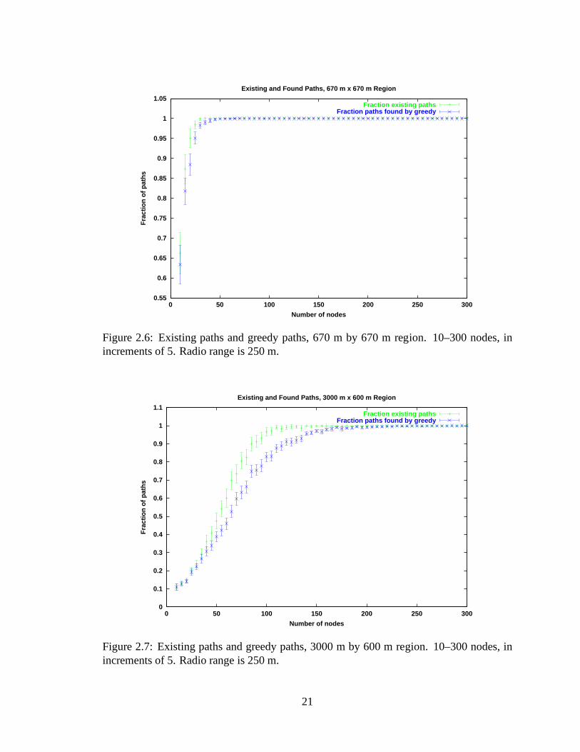
2.6 Existing paths and greedy paths, 670 m by 670 m region. 10–300 nodes, in
increments of 5. Radio range is 250 m. . . . . . . . . . . . . . . . . . . . .21
2.7 Existing paths and greedy paths, 3000 m by 600 m region. 10–300 nodes,
in increments of 5. Radio range is 250 m. . . . . . . . . . . . . . . . . . .21
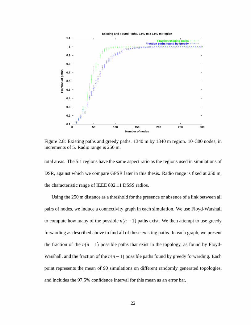
2.8 Existing paths and greedy paths. 1340 m by 1340 m region. 10–300 nodes,
in increments of 5. Radio range is 250 m. . . . . . . . . . . . . . . . . . .22
3.1 The right-hand rule. . . . . . . . . . . . . . . . . . . . . . . . . . . . . . .25
3.2 Right-hand rule forwarding pseudocode. . . . . . . . . . . . . .. . . . . . 26
3.3 A network with crossing edges. . . . . . . . . . . . . . . . . . . . . . .. . 27
viii
3.4 The GPP (Greedy Perimeter Probing) algorithm:PERI-CLOSER-LOOKUP
andGPP-FORWARD. . . . . . . . . . . . . . . . . . . . . . . . . . . . . . . 31
3.5 Mixed forwarding. . . . . . . . . . . . . . . . . . . . . . . . . . . . . . . 32
3.6 Percentage of alln2 routesnot found, GPP. . . . . . . . . . . . . . . . . . . 33
3.7 State per router, GPPvs.Distance-Vector. . . . . . . . . . . . . . . . . . . 34
3.8 Failure of the no-crossing rule. . . . . . . . . . . . . . . . . . . . .. . . . 37
3.9 Perimeter with no closer node, but with an edge containing a closer point. . 37
3.10 The RNG graph. . . . . . . . . . . . . . . . . . . . . . . . . . . . . . . . . 40
3.11 The GG graph. . . . . . . . . . . . . . . . . . . . . . . . . . . . . . . . . 42
3.12 Full, GG subset, and RNG subset radio graphs. . . . . . . . . .. . . . . . 43
3.13 Perimeter forwarding example. . . . . . . . . . . . . . . . . . . . .. . . . 46
3.14 Pseudocode for GPSR. . . . . . . . . . . . . . . . . . . . . . . . . . . . . 49
4.1 Packet Delivery Success Rate. GPSR with varying beacon intervals,B,
compared with DSR. 50 nodes. . . . . . . . . . . . . . . . . . . . . . . . . 62
4.2 Routing Protocol Overhead. Total routing protocol packets sent network-
wide during the simulation for GPSR with varying beacon intervals, B,
compared with DSR. 50 nodes. . . . . . . . . . . . . . . . . . . . . . . . . 64
4.3 Path length beyond optimal for GPSR’s and DSR’s successfully delivered
packets. 50 nodes. . . . . . . . . . . . . . . . . . . . . . . . . . . . . . . . 65
4.4 Packet Delivery Success Rate. For GPSR withB = 1:5 compared with
DSR. 112 nodes. . . . . . . . . . . . . . . . . . . . . . . . . . . . . . . . 69
ix
4.5 Routing Protocol Overhead. Total routing protocol packets sent network-
wide during the simulation for GPSR withB = 1:5 compared with DSR.
112 nodes. . . . . . . . . . . . . . . . . . . . . . . . . . . . . . . . . . . . 70
4.6 Packet Delivery Success Rate. For GPSR withB = 1:5 compared with
DSR. 200 nodes. . . . . . . . . . . . . . . . . . . . . . . . . . . . . . . . 70
4.7 Routing Protocol Overhead. Total routing protocol packets sent network-
wide during the simulation for GPSR withB= 1:5 compared with DSR.y
axis log-scaled. 200 nodes. . . . . . . . . . . . . . . . . . . . . . . . . . . 71
4.8 Path length beyond optimal for GPSR’s and DSR’s successfully delivered
packets. 112 nodes. . . . . . . . . . . . . . . . . . . . . . . . . . . . . . . 72
4.9 Path length beyond optimal for GPSR’s and DSR’s successfully delivered
packets. 200 nodes. . . . . . . . . . . . . . . . . . . . . . . . . . . . . . . 73
4.10 Packet Delivery Success Rate. For GPSR withB = 1:5 compared with
DSR. 50 nodes, sparse topology. . . . . . . . . . . . . . . . . . . . . . . . 75
4.11 Routing Protocol Overhead. Total routing protocol packets sent network-
wide during the simulation for GPSR withB = 1:5 compared with DSR.
50 nodes, sparse topology. . . . . . . . . . . . . . . . . . . . . . . . . . . 77
4.12 Path length beyond optimal for GPSR’s and DSR’s successfully delivered
packets. 50 nodes, sparse topology. . . . . . . . . . . . . . . . . . . . .. . 78
4.13 Average state size stored, 200-node, pause-time-0 simulations, DSRvs.GPSR.
Left: nodes stored; right: bytes stored. . . . . . . . . . . . . . . . .. . . . 80
5.1 An inner perimeter closing around a packet. . . . . . . . . . . .. . . . . . 83
x
There is nothing better for a man,than that he should eat and drink,and that he should make his soul
enjoy good in his labor.Ecclesiastes, 2:24
And further, by these, my son, be admonished:of making many books there is no end;
and much study is a weariness of the flesh.Ecclesiastes, 12:12
Der Mannuberlegt und fragt dann,ob er also spater werde eintreten durfen.
“Es ist moglich,” sagt der Turhuter, “jetzt aber nicht.”. . .
“Wenn es so dich lockt, versuche es doch,trotz meines Verbotes hineinzugehn.
Merke aber: ich bin machtig.Und ich bin nur der unterste Turhuter.
Von Saal zu Saal ist stehn aber Turhuter,einer machtiger als der andere.
Schon den Anblick des dritten kannnicht einmal ich mehr ertragen.”
Franz Kafka,Vor dem Gesetz, in Der Prozeß
Acknowledgements
H. T. Kung, my thesis advisor, taught me the lesson I needed most to learn: that research
requires a sometimes paradoxical combination of critical,truly long-term thinking when
evaluating and directing one’s own work, with an inner confidence that one can, with suffi-
cient dedication over time, contribute. Would that I could learn to duplicate his boundless
energy. The high standards he has imparted to me will benefit my research efforts my whole
life long.
Michael Mitzenmacher, my thesis committee member, made himself available for many
chats, often precipitated by my dropping by his office unexpectedly, about the content and
xi
presentation of this thesis. I always left these chats with aclearer understanding—and a
more clearly and precisely written thesis—than I’d had whenI arrived. Mike Smith, my
other committee member, has unstintingly offered sound advice over the years. His calm,
wisdom, and focus are a potent instance of advising by example.
I have been incredibly fortunate to have had labmates who arenot merely stellar com-
puter scientists—they are also wonderful friends. The hours of creative discussion, arguing,
meals, and pure hilarity I’ve shared with Robert Morris, Dong Lin, Trevor Blackwell, and
Koling Chang have been priceless, and seem entirely too few.May the Bonehed Consor-
tium never fall!
I am especially grateful for the friendship of Robert Morris. Since our first year in lab,
on the day I introduced myself to him, and to break the ice rendered into English the most
shocking joke I’d heard just days before in France, I’ve enjoyed so many discussions that
have shaped and enriched my view of systems and networks. Hisinsight benefitted this
thesis, as well.
Allison Mankin generously supported my research efforts for two years. But beyond
that, the support she provided in the way of technical discussions, advice, and friendship
were invaluable.
I profited immensely from my ten-month visit to ACIRI, endingin May 2000, during
which I developed much of the latter part of this thesis. MarkHandley made my visit
possible initially, and Scott Shenker gave me the chance to stay much longer thereafter.
Dick Karp first suggested I investigate planar graphs, and this thesis benefitted generally
from many discussions with Mark Handley, Scott Shenker, andthe rest of ACIRI.
xii
Chapter 1
Introduction
In networks comprised entirely of wireless stations, communication between source and
destination nodes may require traversal of multiple hops, as radio ranges are limited. Tra-
ditional approaches to therouting problemof finding a sequence of hops between the orig-
inator of a packet and the packet’s destination work by modeling the network as a graph,
and computing all-pairs shortest paths on the edge weights of this graph. These distributed
shortest-path routing algorithms describe the entire topology of the network, or a digest
of it, to all routers on the network to find correct routes. On wired networks, such a re-
quirement is intuitive, in the sense that wired links may be of arbitrary length, and may be
placed in any arbitrary configuration among nodes, independently of the physical distance
between nodes. Thus, one must search over the entire topological description of the net-
work to be certain to find a path that exists. However, this communication of the network’s
topology to all nodes comes at the cost of routing protocol traffic. Moreover, routers need
up-to-date topological information to find correct routes,so in the worst case, changes in
1
topology must be promptly described to all nodes in the network. On a properly function-
ing wired network, changes in the topology are infrequent; they are caused by node or link
failures, or by decommissioning of old links or instatementof new ones. On wireless net-
works, however, the network topology varies frequently in the course of normal operation;
mobility of nodes results in a constantly changing network topology, as nodes move into
and out of one another’s radio ranges.
A community of ad-hoc network researchers has proposed, implemented, and mea-
sured a variety of routing algorithms for such mobile, wireless networks. While these
ad-hoc routing algorithms are designed to generate less routing protocol traffic than the
above-mentioned shortest-path routing protocols in the face of a changing topology, they
nevertheless compute shortest-path routes using either topological information concerning
the entire network, or topological information concerningthe entire set of currently used
paths between sources and destinations. Thus, their ability to find routes depends similarly
on describing the current wide-area topology of the networkto routers.
We propose a different strategy for routing on wireless networks than these traditional
routing algorithms and ad-hoc routing algorithms use. The central approach in this thesis
is to make routing decisions using thegeographic positionsof nodes in the network, as
first suggested by Nelson and Kleinrock [31], Hou and Li [15],and Finn [10]. By using
geographic forwarding, we exploit the facts that:� As the density of nodes on a wireless network increases, shortest paths between
sources and destinations correspond increasingly closelyto the Euclidean straight
line between them.
2
� On wireless networks, the positions ofgeographically nearbynodes determine which
links exist.
Intuitively, leveraging this inherent structure in wireless networks can localize the por-
tion of the network topology that must be described to routers in a routing protocol. Local-
izing the topological information that must be communicated among routers in a routing
protocol improves the scaling of routing in three ways: it reduces the absolute volume of
routing protocol message traffic, reduces the size of the state that must be stored at routers,
and reduces the risk that state stored at a router concerninga far-away portion of the topol-
ogy will become stale. We propose Greedy Perimeter Stateless Routing (GPSR), a routing
protocol for wireless networks, which makes geographic forwarding decisions, and finds
routes using knowledge at each node ofonly that node’s immediate single-hop neighbors
in the topology.
1.1 Metrics for Evaluating Routing Scalability
Our aim is to show that GPSR is a highlyscalablerouting protocol. We aim for scalability
under increasing numbers of nodes in the network, and increasing mobility rate. As these
factors increase, our measures of scalability are:� Routing protocol message cost: How many routing protocol packets does a routing
algorithm send? This metric represents the overhead of routing—the reduction in
network capacity for user data surrendered to maintenance of correct routes.� Application packet delivery success rate: What fraction ofapplications’ packets are
3
delivered successfully by a routing algorithm? This metricrepresents the useful work
done by a routing algorithm.� Path length: How long are the routes found by a routing algorithm, in comparison
with the optimal shortest paths in the network graph? This metric represents how the
latency experienced by applications’ packets compares with the shortest possible.
On wireless networks with fixed transmitter power (e.g., today’s commodity IEEE
802.11 (WaveLAN) radios), this metric also reveals the radio power consumed to
deliver a packet from the source to the destination. In the case of GPSR, where we
use topological information concerning only a node’s immediate neighbors to make
packet forwarding decisions, measuring path length reveals how much optimality is
sacrificed to avoid routing protocol overhead.� Per-node state: How much storage does a routing algorithm require at each node?
This metric is somewhat untraditional in the routing protocol literature. However, on
wireless networks comprised of resource-impoverished devices, such as low-power
sensors, keeping small state at each node is essential, evenwhen the number of de-
ployed sensors in a network is vast.
1.2 Traditional Shortest-Path Algorithms
The two main categories of shortest-path routing algorithms, Distance-Vector (DV, also
known as Distributed Bellman-Ford, DBF) [14] and Link-State (LS) [28] algorithms, re-
quire continual distribution of a current map of the entire network’s topology to all routers.
4
DV’s Bellman-Ford approach constructs this global picturetransitively; each router in-
cludes its distance (the sum of the edge weights between it and the destination) from all
network destinations in each of its periodic beacons. Receipt of a beacon containing a rout-
ing table entry for a destination implies that the receiver can route to that destination via the
neighbor from whom that beacon was received, at a cost equal to the sum of the distance in
the routing table entry and cost of the link over which the beacon was received. Over time,
the route for a destination propagates outward by one hop each time a router sends its next
beacon after learning a route for that new destination. After enough beaconing rounds, all
nodes learn routes for all destinations they can reach.
LS’s Dijkstra approach directly floods announcements of thechange in any link’s status
to every router in the network. Each router keeps a map of the entire network graph, and
runs Dijkstra’s algorithm on this graph map.
Small inaccuracies in the state at a router under both DV and LS can cause routing
loops or disconnection [42]. When the topology is in constant flux, as under mobility,
LS generates torrents of link status change messages, and DVeither suffers from out-of-
date state [7], or generates torrents of triggered updates—messages sent upon change of a
metric for a destination, before the full inter-beacon interval has passed.
1.3 Ad-Hoc Routing Algorithms
A wide variety of ad-hoc routing algorithms have been proposed in the literature. By way
of introduction, we focus on Dynamic Source Routing (DSR) [18]; we compare GPSR
with DSR later in the thesis, because DSR has been shown to perform better than many
5
other published routing algorithms [7]. In DSR, packets arerouted usingsource routes;
each packet contains the full sequence of hops it is to take from the source node to the
destination node. Forwarding such a packet amounts to finding the next hop in the list
of hops, and sending the packet to the appropriate neighbor.The task of writing the full
route into the packet falls to the packet’s originator. If a node originates a packet, and does
not already know a route to the destination, it floods aroute requestpacket to all nodes in
the network. As a route request propagates, it records all hops it traverses. When a route
request reaches the destination, the destination node replies to the request’s originator with
the reversed list of hops accumulated by the request. This reversed list is the source route
from the source to the destination. Note that DSR only generates routing protocol traffic in
response to demand for forwarding to an unknown destination. Thus, DSR is anon-demand
routing protocol, whereas traditional DV and LS algorithmsarepro-active, and continually
describe the topology to all nodes the network.
When a source route to a destination breaks, because two adjacent nodes in the source
route cease to be neighbors, the node who no longer has the next-hop neighbor sends a
route error to the packet’s originator. In response, the packet’s originator re-queries to
learn up-to-date source routes for the destination.
To reduce the traffic load of route queries, all nodes aggressively cacheall routes they
overhear. When a route request arrives for a destination in the route cache, a route re-
ply is sent to the requestor without propagating the route request further. We discuss the
implications of this caching behavior in the next section.
6
1.4 Techniques for Routing Scalability
The two dominant factors in the scaling of both traditional shortest-path routing algorithms
and ad-hoc routing algorithms like DSR are:� The rate of change of the topology.� The number of routers in the routing domain.
Both factors affect the message complexity of DV and LS routing algorithms: intu-
itively, pushing current state globally costs packets proportional to the product of the rate
of state change and number of destinations for the updated state. In the case of DSR, source
routes break more frequently as mobility increases, and theprobability that a source route
breaks increases as the network diameter increases.
Two main approaches are used in an attempt to mitigate the influence of these two
factors in limiting the scalability of routing protocols:� Hierarchy is the most widely deployed approach to scale routing as the number of
network destinations increases. Without hierarchy, Internet routing could not scale to
support today’s number of Internet leaf networks. An Autonomous System runs an
intra-domain routing protocol inside its borders, and appears as a single entity in the
backbone inter-domain routing protocol, BGP. This hierarchy is built on well-defined
and rarely changing administrative and topological boundaries.The assumptions that
such static boundaries exist, and that a common administrative authority can set
them, are incorrect on freely moving ad-hoc wireless networks.
7
� Cachinghas come to prominence as a strategy for scaling ad-hoc routing protocols.
Dynamic Source Routing (DSR) [18], Ad-Hoc On-Demand Distance Vector Routing
(AODV) [33], and the Zone Routing Protocol (ZRP) [13] all eschew constantly push-
ing current topology information network-wide. Instead, routers running these pro-
tocols request topological information in anon-demandfashion as required by their
packet forwarding load, and cache it aggressively. When their cached topological
information becomes out-of-date, these routers must obtain more current topological
information to continue routing successfully. Caching reduces the routing protocols’
message load in two ways: it avoids pushing topological information where the for-
warding load does not require it (e.g.,at idle routers), and it often reduces the number
of hops between the router that has the needed topological information and the router
that requires it (i.e., a node closer than a changed link may already have cached the
new status of that link).Caching in computer systems is predicated on the assump-
tion that cached values remain valid long enough to be reusedbefore becoming stale.
This assumption becomes invalid as mobility and the length of a route increase in the
limit; the probability that a cached route remains correct is inversely proportional to
the product of the mobility rate and path length.
1.5 Applicability of Scalable Wireless Routing
Wireless networks that push on mobility, number of nodes, orboth include:� Ad-hoc networks: Perhaps the most investigated category, these mobile networks
have no fixed infrastructure, and support applications for military users, post-disaster
8
rescuers, and temporary collaborations among temporary associates, as at a business
conference or lecture [13], [18], [32], [33], [34].� Sensor networks: Comprised of small sensors, these mobile networks can be de-
ployed with very large numbers of nodes, and have very impoverished per-node re-
sources [9], [19]. Minimization of state per node in a network of tens of thousands
of memory-poor sensors is crucial.� “Rooftop” networks: Proposed by Shepard [37], these wireless networks are not
mobile, but are deployed very densely in metropolitan areas(the name refers to an
antenna on each building’s roof, for line-of-sight with neighbors) as an alternative
to wired networking offered by traditional telecommunications providers. Such a
network also provides an alternate infrastructure in the event of failure of the con-
ventional one, as after a disaster. A routing system that self-configures (without a
trusted authority to configure a routing hierarchy) for hundreds of thousands of such
nodes in a metropolitan area represents a significant scaling challenge.� Vehicular networks: These networks consist of moving vehicles equipped with ra-
dios [29]. Both peer-to-peer communication, as for music sharing and driver-to-
driver communication, and Internet access infrastructureuses, in which vehicles
reach base stations connected to the Internet via routes through other vehicles, are
useful applications on such networks. The availability of the vehicle battery as a
power source, recharged by generation of current from the vehicle’s propulsion sys-
tem, eliminates the need for concern about battery life limitations at nodes.
9
1.6 Assumptions
We assume in this work that all wireless routers know their own positions, either from a
GPS device, if outdoors, or through other means. Practical solutions include surveying,
for stationary wireless routers; inertial sensors, on vehicles, as are commonly deployed in
car mapping and navigation systems; and acoustic range-finding using ultrasonic “chirps”
indoors [41], [35]. We further assume bidirectional radio reachability. The widely used
IEEE 802.11 wireless network MAC [17] sends link-level acknowledgements for all uni-
cast packets, so that all links in an 802.11 network must be bidirectional. We simulate a
network that uses 802.11 radios to evaluate our routing protocol. We consider topologies
where the wireless nodes are roughly in a plane. We assume that the distance between
nodes determines whether a link exists between them; below acertain distance threshold,
two nodes are within range of one another. Finally, we assumethat packet sources can
determine the approximate locations (to within a radio range) of packet destinations, to
mark packets they originate with their destination’s location. Thus, we assume a location
registration and lookup service that maps node addresses tolocations [25]. Queries to this
system use thesamegeographic routing system as data packets; the querier geographically
addresses his request to a location server. The scope of thisthesis is limited to geographic
routing. We discuss interaction with the location service briefly in Section 5.2. A technique
for correcting for inaccuracy in the position of the destination is presented in Section 5.3.
We adopt IP terminology throughout, though GPSR can be applied to any datagram net-
work.
10
1.7 Thesis Contents
We will show that geographic routing allows routers to be nearly stateless, and requires
propagation of topology information for only asingle hop: each node need only know
its neighbors’ positions. The self-describing nature of position is the key to geography’s
usefulness in routing. The position of a packet’s destination and positions of the candidate
next hops are sufficient to make correct forwarding decisions, without any other topological
information. This self-describing property of geographicaddresses is in contrast with usual
flat network addresses (as in the “default-free” core of the Internet), the internal structure
of which does not assist in making forwarding decisions, such that routers must make table
lookups to choose a next hop.
In Chapter 2, we describe a simple greedy geographic forwarding algorithm, discuss
the scalability implications of its design, and evaluate the algorithm’s degree of success
in finding routes on static, non-mobile wireless networks. This greedy algorithm does not
always find paths successfully; we characterize the topologies on which this is the case.
In Chapter 3, motivated by the failures of greedy forwarding, we propose two meth-
ods for recovering from greedy forwarding failure. The firstmethod, perimeter probing,
uses a heuristic to remove crossing links from the wireless network, and finds most routes
successfully, but not all. We characterize the topologies where perimeter probing fails to
find routes. The second method, planarization of the graph, finds all routes successfully
on static networks. We then present the full GPSR algorithm,which combines greedy for-
warding where topology allows, with forwarding along perimeters of the planarized graph,
where greedy forwarding is impossible.
11
In Chapter 4, we evaluate GPSR in simulation on dense mobile wireless networks of
50, 112, and 200 nodes, at varying degrees of motion, including simulation of the full
IEEE 802.11 physical and MAC layers, using the scalability metrics proposed in this in-
troduction. We also simulate a sparser configuration of nodes. We show that GPSR keeps
tiny state per node, delivers user packets robustly, generates small routing protocol over-
head, and delivers the vast majority of packets in the numberof hops equal to that along
the shortest path. We simulate DSR for comparison on the samenetworks, and show that
GPSR outperforms DSR by these metrics.
In Chapter 5, we discuss the properties of GPSR, and describeavenues for further
extension of the work in this thesis.
We review related work in Chapter 6.
Finally, we conclude in Chapter 7, by reviewing the design ofGPSR, summarizing the
results of our evaluation of GPSR, and stating the contributions of this thesis.
12
Chapter 2
Greedy Forwarding
We now describe the first part of the Greedy Perimeter Stateless Routing algorithm:greedy
forwarding. In this chapter, we define the greedy forwarding rule; definea simple beacon-
ing protocol for nodes to learn their neighbors’ positions;identify the desirable properties
of greedy forwarding; define the topologies on which greedy forwarding fails; and charac-
terize the frequency of greedy forwarding failure by thedensityof nodes in a network.
2.1 Greedy Forwarding Rule
As alluded to in the introduction, under GPSR, packets are marked by their originator with
their destinations’ locations. As a result, a forwarding node can make a locally optimal,
greedy choice in choosing a packet’s next hop. Specifically,if a node knows its radio
neighbors’ positions, the locally optimal choice of next hop is the neighbor geographically
closest to the packet’s destination. Forwarding in this regime follows successively closer
geographic hops, until the destination is reached. An example of greedy next-hop choice
13
y
x
D
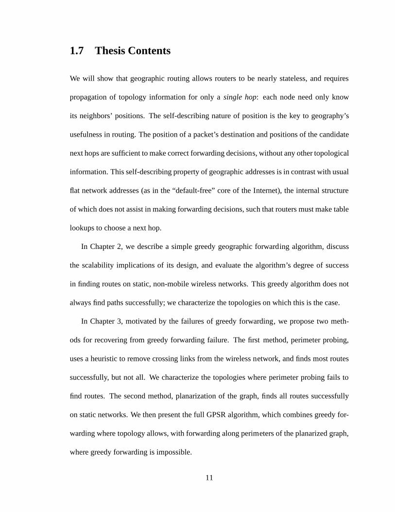
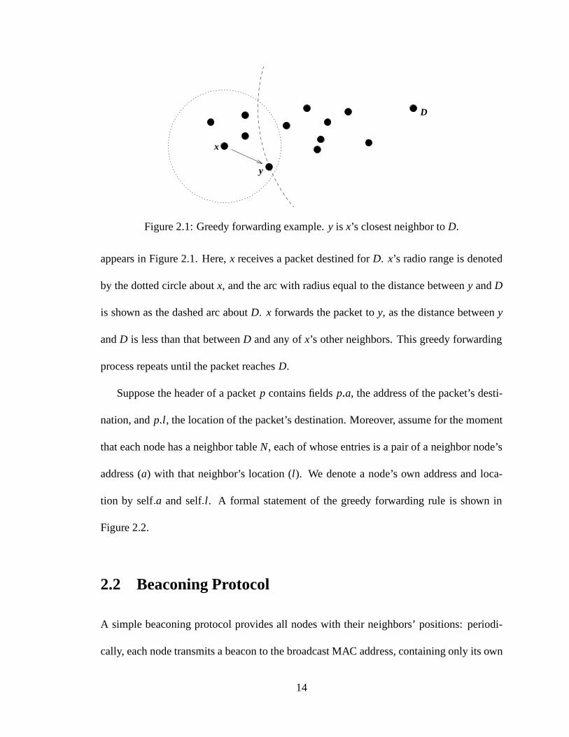
Figure 2.1: Greedy forwarding example.y is x’s closest neighbor toD.
appears in Figure 2.1. Here,x receives a packet destined forD. x’s radio range is denoted
by the dotted circle aboutx, and the arc with radius equal to the distance betweeny andD
is shown as the dashed arc aboutD. x forwards the packet toy, as the distance betweeny
andD is less than that betweenD and any ofx’s other neighbors. This greedy forwarding
process repeats until the packet reachesD.
Suppose the header of a packetp contains fieldsp:a, the address of the packet’s desti-
nation, andp:l , the location of the packet’s destination. Moreover, assume for the moment
that each node has a neighbor tableN, each of whose entries is a pair of a neighbor node’s
address (a) with that neighbor’s location (l ). We denote a node’s own address and loca-
tion by self:a and self:l . A formal statement of the greedy forwarding rule is shown in
Figure 2.2.
2.2 Beaconing Protocol
A simple beaconing protocol provides all nodes with their neighbors’ positions: periodi-
cally, each node transmits a beacon to the broadcast MAC address, containing only its own
14

GREEDY-FORWARD(p)1 nbest= self:a2 dbest= DISTANCE(self:l ; p:l)3 for each (a; l) in N4 do d = DISTANCE(l ; p:l)5 if a== p:a or d < dbest6 then nbest= a7 dbest= d8 if a== p:a9 then break
10 if nbest== self:a11 then return greedy forwarding failure12 else forward p to nbest
13 return greedy forwarding success
Figure 2.2: Greedy forwarding rule pseudocode.DISTANCE(e; f ) computes the Euclideandistance between nodeseand f —in two dimensions,
p(xe�xf )2+(ye�yf )2.
identifier (e.g.,IP address) and position. We encode position as two four-byte floating-point
quantities, forx andy coordinate values. To avoid synchronization of neighbors’beacons,
as observed by Floyd and Jacobson [11], we jitter each beacon’s transmission by 50% of
the intervalB between beacons, such that the mean inter-beacon transmission interval isB,
uniformly distributed in[0:5B;1:5B℄.Upon not receiving a beacon from a neighbor for longer than timeout intervalT, a
GPSR router assumes that the neighbor has failed or gone out-of-range, and deletes the
neighbor from its table. The 802.11 MAC layer also gives direct indications of link-level
retransmission failures to neighbors; we interpret these indications identically. We have
usedT = 4:5B, three times the maximum jittered beacon interval, in this work.
The position a node associates with a neighbor becomes less current between beacons
as that neighbor moves. The accuracy of the set of neighbors also decreases; old neighbors
may leave and new neighbors may enter radio range. For these reasons, the correct choice
15
of beaconing interval to keep nodes’ neighbor tables current depends on the rate of mobility
in the network and range of nodes’ radios. We show the effect of this interval on GPSR’s
performance in our simulation results. We note that keepingcurrent topological state for
a one-hop radius about a router is the minimum required to doany routing; no useful
forwarding decision can be made without knowledge of the topology one or more hops
away.
This beaconing mechanism does represent pro-active routing protocol traffic, avoided
by DSR and AODV. To minimize the cost of beaconing, GPSR piggybacks the local send-
ing node’s position onall data packets it forwards, and runs all nodes’ network interfaces in
promiscuous mode, so that each station receives a copy of allpackets for all stations within
radio range. At a small cost in bytes (twelve bytes per packet), this scheme allows all pack-
ets to serve as beacons. When any node sends a data packet, it can then reset its inter-beacon
timer. This optimization reduces beacon traffic in regions of the network actively forward-
ing data packets. Running network interfaces in promiscuous mode consumes power; we
do not measure power consumption in this work.
In fact, we could make GPSR’s beacon mechanism fully reactive by having nodes solicit
beacons with a broadcast “neighbor request” only when they have data traffic to forward.
We have not felt it necessary to take this step, however, as the one-hop beacon overhead
does not congest our simulated networks.
16
2.3 Advantages of Greedy Forwarding
Greedy forwarding’s great advantage is its reliance only onknowledge of the forwarding
node’s immediate neighbors. The state required is negligible, and dependent on the density
of nodes in the wireless network, not the total number of destinations in the network.1 On
networks where multi-hop routing is useful, the number of neighbors within a node’s radio
range must be substantially less than the total number of nodes in the network.
As mentioned in the Introduction, as the density in space of the nodes deployed on a
wireless network increases, greedy forwarding approximates shortest paths progressively
more closely; the shortest path between two nodes tends toward the Euclidean straight line
between them, as the minimum possible number of hops is bounded below by the number
of radio ranges between source and destination, laid end-to-end.
Traditional shortest-path routing algorithms cannot exploit structure in IP addresses to
make forwarding decisions; they must treat IP addresses as flat identifiers, and resort to a
table lookup among all destinations in the routing domain. It is the self-describing nature of
geographic coordinates that allows forwarding routers to interpret the destination location
in a packet to make a purely local forwarding decision.
Note that the only routing protocol traffic required for greedy forwarding is that of the
beaconing protocol. Because the beaconing protocol pushesstate only a single hop in the
network, intuitively it should consume considerably less bandwidth than protocols which
distribute state globally throughout the routing domain (e.g.,DV and LS routing protocols),
or accumulate state along an entire source route (e.g.,DSR).
1The word “stateless” in GPSR’s name is not meant literally, but refers to this small, purely local state.
17

Because greedy forwarding makes purely local decisions, itshould be robust under
topological changes; a node can make correct forwarding decisions without requiring up-
to-date state (or indeed, any state) concerning nodes beyond a single hop away.
2.4 Limits to Greedy Forwarding’s Applicability: Voids
The power of greedy forwarding to route using only neighbor nodes’ positions comes
with one attendant drawback: there are topologies in which the only route to a destina-
tion requires a packet move temporarilyfarther in geometric distance from the destina-
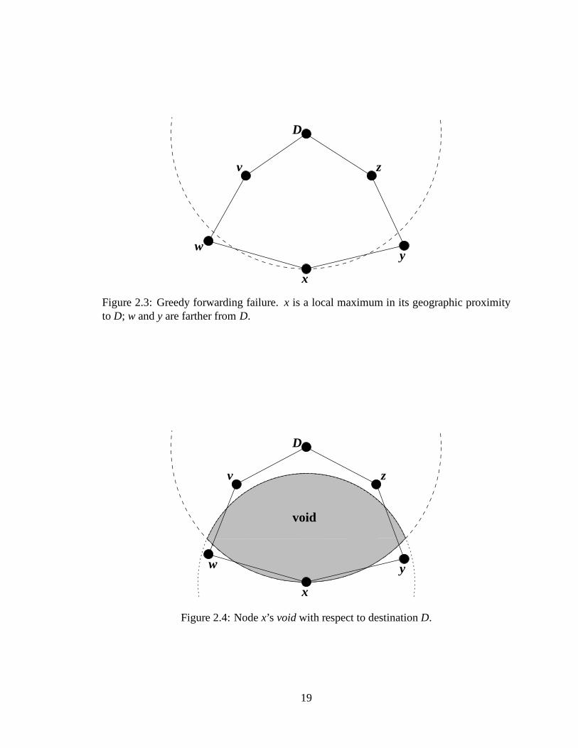
tion [10], [22]. A simple example of such a topology is shown in Figure 2.3. Here,x is
closer toD than its neighborsw andy. Again, the dashed arc aboutD has a radius equal to
the distance betweenx andD. Although two paths,(x! y! z!D) and(x!w! v!D),exist toD, x will not choose to forward tow or y using greedy forwarding.x is a local max-
imum in its proximity toD. Some other mechanism must be used to forward packets in
these situations.
Motivated by Figure 2.3, we note that theintersectionof x’s circular radio range and
the circle aboutD of radiusjxDj (that is, of the length of line segmentxD) is empty of
neighbors. We show this region clearly in Figure 2.4. From nodex’s perspective, we term
the shaded region without nodes avoid. x seeks to forward a packet to destinationD beyond
the edge of this void. Intuitively,x seeks to routearoundthe void; if a path toD exists from
x, it doesn’t include nodes located within the void (orx would have forwarded to them
greedily).
18
x
wy
D
zv
Figure 2.3: Greedy forwarding failure.x is a local maximum in its geographic proximityto D; w andy are farther fromD.
D
v z
w
x
y
void
Figure 2.4: Nodex’s voidwith respect to destinationD.
19
0.4
0.5
0.6
0.7
0.8
0.9
1
1.1
0 50 100 150 200 250 300
Fra
ctio
n o
f p
ath
s
Number of nodes
Existing and Found Paths, 1500 m x 300 m Region
Fraction existing pathsFraction paths found by greedy
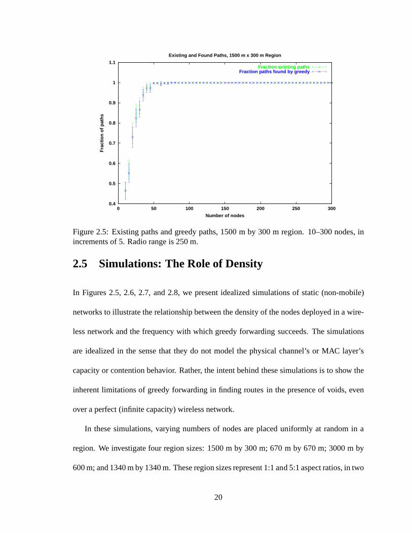
Figure 2.5: Existing paths and greedy paths, 1500 m by 300 m region. 10–300 nodes, inincrements of 5. Radio range is 250 m.
2.5 Simulations: The Role of Density
In Figures 2.5, 2.6, 2.7, and 2.8, we present idealized simulations of static (non-mobile)
networks to illustrate the relationship between the density of the nodes deployed in a wire-
less network and the frequency with which greedy forwardingsucceeds. The simulations
are idealized in the sense that they do not model the physicalchannel’s or MAC layer’s
capacity or contention behavior. Rather, the intent behindthese simulations is to show the
inherent limitations of greedy forwarding in finding routesin the presence of voids, even
over a perfect (infinite capacity) wireless network.
In these simulations, varying numbers of nodes are placed uniformly at random in a
region. We investigate four region sizes: 1500 m by 300 m; 670m by 670 m; 3000 m by
600 m; and 1340 m by 1340 m. These region sizes represent 1:1 and 5:1 aspect ratios, in two
20
0.55
0.6
0.65
0.7
0.75
0.8
0.85
0.9
0.95
1
1.05
0 50 100 150 200 250 300
Fra
ctio
n o
f p
ath
s
Number of nodes
Existing and Found Paths, 670 m x 670 m Region
Fraction existing pathsFraction paths found by greedy
Figure 2.6: Existing paths and greedy paths, 670 m by 670 m region. 10–300 nodes, inincrements of 5. Radio range is 250 m.
0
0.1
0.2
0.3
0.4
0.5
0.6
0.7
0.8
0.9
1
1.1
0 50 100 150 200 250 300
Fra
ctio
n o
f p
ath
s
Number of nodes
Existing and Found Paths, 3000 m x 600 m Region
Fraction existing pathsFraction paths found by greedy
Figure 2.7: Existing paths and greedy paths, 3000 m by 600 m region. 10–300 nodes, inincrements of 5. Radio range is 250 m.
21
0.1
0.2
0.3
0.4
0.5
0.6
0.7
0.8
0.9
1
1.1
0 50 100 150 200 250 300
Fra
ctio
n o
f p
ath
s
Number of nodes
Existing and Found Paths, 1340 m x 1340 m Region
Fraction existing pathsFraction paths found by greedy
Figure 2.8: Existing paths and greedy paths. 1340 m by 1340 m region. 10–300 nodes, inincrements of 5. Radio range is 250 m.
total areas. The 5:1 regions have the same aspect ratio as theregions used in simulations of
DSR, against which we compare GPSR later in this thesis. Radio range is fixed at 250 m,
the characteristic range of IEEE 802.11 DSSS radios.
Using the 250 m distance as a threshold for the presence or absence of a link between all
pairs of nodes, we induce a connectivity graph in each simulation. We use Floyd-Warshall
to compute how many of the possiblen(n�1) paths exist. We then attempt to use greedy
forwarding as described above to find all of these existing paths. In each graph, we present
the fraction of then(n� 1) possible paths that exist in the topology, as found by Floyd-
Warshall, and the fraction of then(n�1) possible paths found by greedy forwarding. Each
point represents the mean of 90 simulations on different randomly generated topologies,
and includes the 97.5% confidence interval for this mean as anerror bar.
22
All four region sizes demonstrate the same trend: greedy forwarding tends to find all
routes on the sparsest networks and the densest networks, but fails to find some routes
in a middle range of node densities. On very sparse networks,there are so few nodes,
and hence routes on average consist of so few hops, that voidsare very rarely on a path
between a source and a destination. Note from the previous section that voids occur when
two overlapping circles are empty of nodes. The probabilitythat this overlapping region is
empty decreases as nodes become thicker on the ground. Hence, greedy forwarding tends
toward finding all routes as the density of nodes increases.
The aspect ratio of the region has an effect on the success rate of greedy forwarding in
finding routes. In the 1500-m-by-300-m simulations (Figure2.5), the vertical dimension
of the simulated region is not much longer than the 250 m radiorange. Very few voids can
exist in such a region, where one node’s radio range covers nearly the entirey dimension
of the region. Hence, greedy forwarding finds a greater proportion of the existing routes in
this region than in the others measured.
23
Chapter 3
The Right-Hand Rule: Perimeters
In this chapter, we address the failure of pure greedy routing to find paths in the presence
of voids, by introducing twoperimeter traversalalgorithms for forwarding packetsaround
voids. After describing theright-hand rulefor traversing a graph, we characterize the be-
havior of the right-hand rule on wireless network graphs, and observe the role played by
crossing edges in the graph in interfering with the right-hand-rule traversal. We then in-
troduceperimeter probing, an algorithm that probes and maps the positions of nodes that
border voids, while employing ano-crossing heuristicto eliminate crossing edges from
the graph, and uses the resulting state to forward around voids. Drawing on existing re-
sults from computational geometry, we describe theGabriel GraphandRelative Neigh-
borhood Graphplanar graphs, and introduce distributed algorithms for identifying these
graphs as subsets of a wireless network graph. Finally, after describing the topologies on
which perimeter probing fails to find routes, we introduce a superior algorithm,planar face
traversal, that findsall routes on a static network by forwarding only on planar subsets of
24
y
3.1.
2.x z
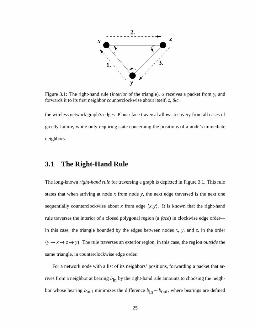
Figure 3.1: The right-hand rule (interior of the triangle).x receives a packet fromy, andforwards it to its first neighbor counterclockwise about itself, z, &c.
the wireless network graph’s edges. Planar face traversal allows recovery from all cases of
greedy failure, while only requiring state concerning the positions of a node’s immediate
neighbors.
3.1 The Right-Hand Rule
The long-knownright-hand rulefor traversing a graph is depicted in Figure 3.1. This rule
states that when arriving at nodex from nodey, the next edge traversed is the next one
sequentially counterclockwise aboutx from edge(x;y). It is known that the right-hand
rule traverses the interior of a closed polygonal region (aface) in clockwise edge order—
in this case, the triangle bounded by the edges between nodesx, y, andz, in the order(y! x! z! y). The rule traverses an exterior region, in this case, the region outsidethe
same triangle, in counterclockwise edge order.
For a network node with a list of its neighbors’ positions, forwarding a packet that ar-
rives from a neighbor at bearingbin by the right-hand rule amounts to choosing the neigh-
bor whose bearingbout minimizes the differencebin�bout, where bearings are defined
25
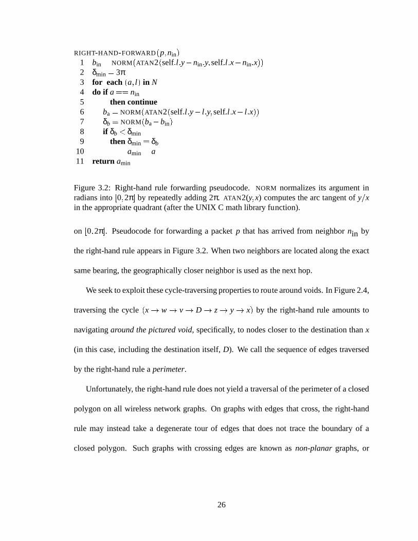
RIGHT-HAND-FORWARD(p;nin)1 bin = NORM(ATAN 2(self:l :y�nin:y;self:l :x�nin:x))2 δmin = 3π3 for each (a; l) in N4 do if a== nin
5 then continue6 ba = NORM(ATAN 2(self:l :y� l :y;self:l :x� l :x))7 δb = NORM(ba�bin)8 if δb < δmin9 then δmin = δb
10 amin = a11 return amin
Figure 3.2: Right-hand rule forwarding pseudocode.NORM normalizes its argument inradians into[0;2π℄ by repeatedly adding 2π. ATAN 2(y;x) computes the arc tangent ofy=xin the appropriate quadrant (after the UNIX C math library function).
on [0;2π℄. Pseudocode for forwarding a packetp that has arrived from neighbornin by
the right-hand rule appears in Figure 3.2. When two neighbors are located along the exact
same bearing, the geographically closer neighbor is used asthe next hop.
We seek to exploit these cycle-traversing properties to route around voids. In Figure 2.4,
traversing the cycle(x! w! v! D ! z! y! x) by the right-hand rule amounts to
navigatingaround the pictured void, specifically, to nodes closer to the destination thanx
(in this case, including the destination itself,D). We call the sequence of edges traversed
by the right-hand rule aperimeter.
Unfortunately, the right-hand rule does not yield a traversal of the perimeter of a closed
polygon on all wireless network graphs. On graphs with edgesthat cross, the right-hand
rule may instead take a degenerate tour of edges that does nottrace the boundary of a
closed polygon. Such graphs with crossing edges are known asnon-planargraphs, or
26
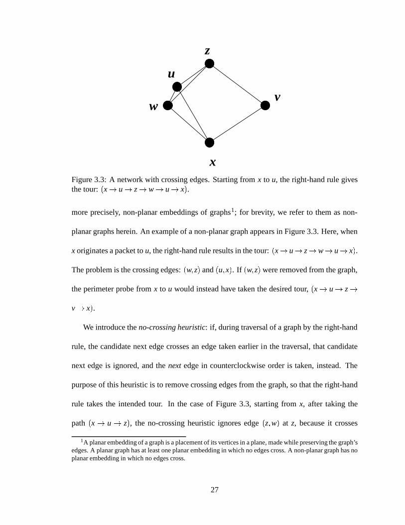
z
x
u
vw
Figure 3.3: A network with crossing edges. Starting fromx to u, the right-hand rule givesthe tour:(x! u! z! w! u! x).more precisely, non-planar embeddings of graphs1; for brevity, we refer to them as non-
planar graphs herein. An example of a non-planar graph appears in Figure 3.3. Here, when
x originates a packet tou, the right-hand rule results in the tour:(x! u! z!w! u! x).The problem is the crossing edges:(w;z) and(u;x). If (w;z) were removed from the graph,
the perimeter probe fromx to u would instead have taken the desired tour,(x! u! z!v! x).
We introduce theno-crossing heuristic: if, during traversal of a graph by the right-hand
rule, the candidate next edge crosses an edge taken earlier in the traversal, that candidate
next edge is ignored, and thenextedge in counterclockwise order is taken, instead. The
purpose of this heuristic is to remove crossing edges from the graph, so that the right-hand
rule takes the intended tour. In the case of Figure 3.3, starting from x, after taking the
path (x! u! z), the no-crossing heuristic ignores edge(z;w) at z, because it crosses
1A planar embedding of a graph is a placement of its vertices ina plane, made while preserving the graph’sedges. A planar graph has at least one planar embedding in which no edges cross. A non-planar graph has noplanar embedding in which no edges cross.
27
the previously taken edge(x;u). Here, the heuristic has the desired effect: the complete
clockwise outer edge tour(x! u! z! v! x) is taken. The implementation of this
heuristic is straightforward: each node appends its location to packets it forwards by the
right-hand rule, and checks whether a candidate next edge crosses one already taken in the
packet’s path history using simple simultaneous equationsfor the two edges in question.
We omit these details in Figure 3.2.
3.2 Perimeter Probing
Building on the right-hand rule and no-crossing heuristic,we now describeperimeter prob-
ing, through which nodes pro-actively map the perimeters they border, and use this knowl-
edge of the local topology to attempt to recover from greedy forwarding failure by routing
around voids.
3.2.1 Greedy Perimeter Probing (GPP) Algorithm
In the topology in Figure 2.4, supposex sends aperimeter probepacket tow. At each hop,
the packet is forwarded using the right-hand rule with the no-crossing heuristic, and each
forwarding router appends its address and position to the packet. When the packet returns
to x, it will contain a list of the positions and addresses of all nodes on the perimeter. Nodex
consumes the packet and caches this state. A proof that perimeter probe packets forwarded
in this fashion on static network topologiesalwaysreturn to their originator can be found
in [30].
Thereafter, should a packet arrive atx for greedy forwarding toD, x can “fail-over” to
28
use the perimeter it has learned, which includes nodesv, D, andz, all of which are closer to
D thanx. Nodex can either source-route the packet to any node closer toD on the cached
perimeter, or mark the packet for forwarding by the right-hand rule, so that it takes the
same path as the earlier perimeter probe packet. In this way,the packet will reach a node
closer toD thanx, where greedy forwarding can resume.
More generally, we can augment greedy forwarding with perimeter probing, in an ef-
fort to recover from greedy forwarding failure by forwarding along perimeters. All nodes
periodically originate a perimeter probe packet (markedperimeter probein a packetp’s
packet mode field,p:M, as in Table 3.1) to each of their neighbors, and cache the perime-
ters stored in these packets when they return to their originators. Greedy forwarding is
used for all data packets where possible—that is, by all nodes where there exists a neighbor
closer to the destination. When no such neighbor exists, a node searches its cached list of
perimeters for any node closer than itself to the destination. If there is no closer node on
any perimeter, no route is known, and the node drops the packet. If such a closer nodenc
exists along perimeterpc, the packet’s mode fieldp:M is changed toperimeter data, and
the packet is marked inp:i with the location where this mode transition occurred. It isthen
forwarded to the next node alongpc. Each successive node that receives a perimeter-mode
packet forwards the packet by the right-hand rule, until thepacket reaches a node closer to
the destinationp:D than that where it entered perimeter mode (atp:i). At that closer node,
the packet is returned togreedy mode, and greedy forwarding continues thereafter. Thus,
the sequence of hops a packet takes in perimeter mode in the aggregate acts as a single
greedy hop, as the packet reaches a node closer to the destination than the one where it en-
29
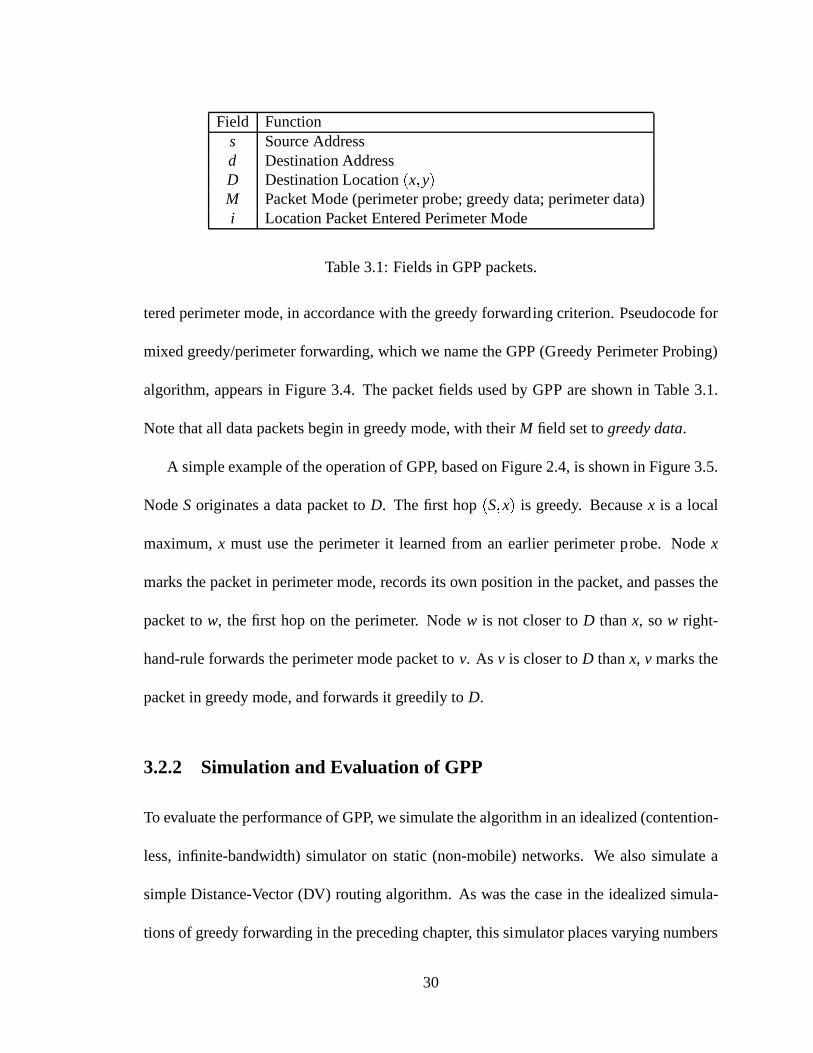
Field Functions Source Addressd Destination AddressD Destination Location(x;y)M Packet Mode (perimeter probe; greedy data; perimeter data)i Location Packet Entered Perimeter Mode
Table 3.1: Fields in GPP packets.
tered perimeter mode, in accordance with the greedy forwarding criterion. Pseudocode for
mixed greedy/perimeter forwarding, which we name the GPP (Greedy Perimeter Probing)
algorithm, appears in Figure 3.4. The packet fields used by GPP are shown in Table 3.1.
Note that all data packets begin in greedy mode, with theirM field set togreedy data.
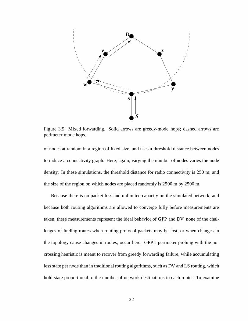
A simple example of the operation of GPP, based on Figure 2.4,is shown in Figure 3.5.
NodeS originates a data packet toD. The first hop(S;x) is greedy. Becausex is a local
maximum,x must use the perimeter it learned from an earlier perimeter probe. Nodex
marks the packet in perimeter mode, records its own positionin the packet, and passes the
packet tow, the first hop on the perimeter. Nodew is not closer toD thanx, sow right-
hand-rule forwards the perimeter mode packet tov. As v is closer toD thanx, v marks the
packet in greedy mode, and forwards it greedily toD.
3.2.2 Simulation and Evaluation of GPP
To evaluate the performance of GPP, we simulate the algorithm in an idealized (contention-
less, infinite-bandwidth) simulator on static (non-mobile) networks. We also simulate a
simple Distance-Vector (DV) routing algorithm. As was the case in the idealized simula-
tions of greedy forwarding in the preceding chapter, this simulator places varying numbers
30
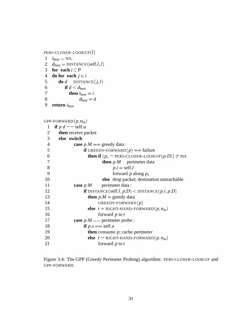
PERI-CLOSER-LOOKUP(l)1 ibest= NIL
2 dbest= DISTANCE(self:l ; l)3 for each i 2 P4 do for each j 2 i5 do d = DISTANCE( j; l)6 if d < dbest7 then ibest= i8 dbest= d9 return ibest
GPP-FORWARD(p;nin)1 if p:d == self:a2 then receive packet3 else switch4 casep:M == greedy data :5 if GREEDY-FORWARD(p) == failure6 then if (pc = PERI-CLOSER-LOOKUP(p:D)) 6= NIL
7 then p:M = perimeter data8 p:i = self:l9 forwardp alongpc
10 else drop packet; destination unreachable11 casep:M == perimeter data :12 if DISTANCE(self:l ; p:D)< DISTANCE(p:i; p:D)13 then p:M = greedy data14 GREEDY-FORWARD(p)15 else t = RIGHT-HAND-FORWARD(p;nin)16 forwardp to t17 casep:M == perimeter probe :18 if p:s== self:a19 then consumep; cache perimeter20 else t = RIGHT-HAND-FORWARD(p;nin)21 forwardp to t
Figure 3.4: The GPP (Greedy Perimeter Probing) algorithm:PERI-CLOSER-LOOKUP andGPP-FORWARD.
31
wy
D
zv
x
S
Figure 3.5: Mixed forwarding. Solid arrows are greedy-modehops; dashed arrows areperimeter-mode hops.
of nodes at random in a region of fixed size, and uses a threshold distance between nodes
to induce a connectivity graph. Here, again, varying the number of nodes varies the node
density. In these simulations, the threshold distance for radio connectivity is 250 m, and
the size of the region on which nodes are placed randomly is 2500 m by 2500 m.
Because there is no packet loss and unlimited capacity on thesimulated network, and
because both routing algorithms are allowed to converge fully before measurements are
taken, these measurements represent the ideal behavior of GPP and DV: none of the chal-
lenges of finding routes when routing protocol packets may belost, or when changes in
the topology cause changes in routes, occur here. GPP’s perimeter probing with the no-
crossing heuristic is meant to recover from greedy forwarding failure, while accumulating
less state per node than in traditional routing algorithms,such as DV and LS routing, which
hold state proportional to the number of network destinations in each router. To examine
32
0
0.001
0.002
0.003
0.004
0.005
0.006
0 50 100 150 200 250 300 350
Fra
ctio
n o
f ro
ute
s n
ot
fou
nd
Number of nodes
GPP
Figure 3.6: Percentage of alln2 routesnot found, GPP.
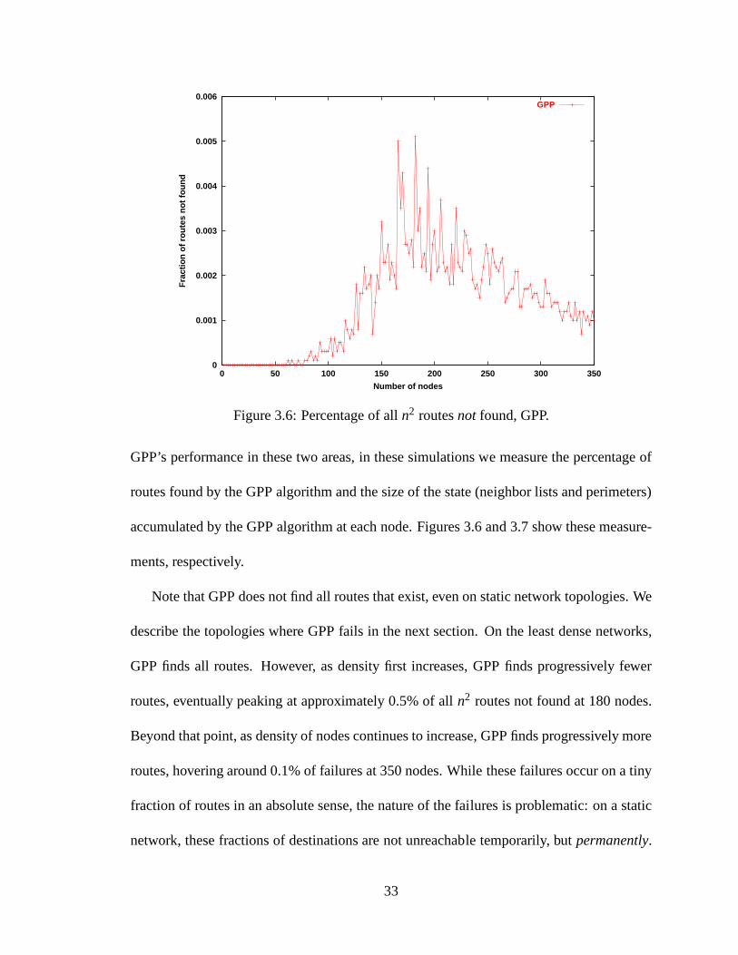
GPP’s performance in these two areas, in these simulations we measure the percentage of
routes found by the GPP algorithm and the size of the state (neighbor lists and perimeters)
accumulated by the GPP algorithm at each node. Figures 3.6 and 3.7 show these measure-
ments, respectively.
Note that GPP does not find all routes that exist, even on static network topologies. We
describe the topologies where GPP fails in the next section.On the least dense networks,
GPP finds all routes. However, as density first increases, GPPfinds progressively fewer
routes, eventually peaking at approximately 0.5% of alln2 routes not found at 180 nodes.
Beyond that point, as density of nodes continues to increase, GPP finds progressively more
routes, hovering around 0.1% of failures at 350 nodes. Whilethese failures occur on a tiny
fraction of routes in an absolute sense, the nature of the failures is problematic: on a static
network, these fractions of destinations are not unreachable temporarily, butpermanently.
33
0
50
100
150
200
250
300
350
0 50 100 150 200 250 300 350
Mea
n s
tate
per
no
de
(in
oth
er n
od
es k
no
wn
)
Number of nodes
GPPDistance-Vector
Figure 3.7: State per router, GPPvs.Distance-Vector.
When allowed to converge fully on an idealized network, DV finds all routes; hence it is
not shown in Figure 3.6. Note that this 100% success rate of DVapplies only to static,
idealized networks; it has been shown that DV routing algorithms find significantly smaller
fractions of the existing routes on mobile, finite-capacitywireless networks [7].
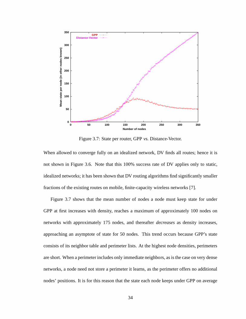
Figure 3.7 shows that the mean number of nodes a node must keepstate for under
GPP at first increases with density, reaches a maximum of approximately 100 nodes on
networks with approximately 175 nodes, and thereafterdecreasesas density increases,
approaching an asymptote of state for 50 nodes. This trend occurs because GPP’s state
consists of its neighbor table and perimeter lists. At the highest node densities, perimeters
are short. When a perimeter includes only immediate neighbors, as is the case on very dense
networks, a node need not store a perimeter it learns, as the perimeter offers no additional
nodes’ positions. It is for this reason that the state each node keeps under GPP on average
34
levels off as the number of nodes increases. In the middle range of densities measured,
perimeters are longer. At the lowest densities measured, perimeters are short because the
number of nodes in the network constrains the number of perimeters a node borders and
the length of those perimeters. DV routing stores state for amean number of nodes less
than the total number of destinations on the sparsest networks, because so many routes are
partitioned on those networks. As density increases, DV routing approaches the expected
state size of the number of network destinations. Note that only after density increases
enough to connect most of the network graph, at approximately 150 nodes total, does GPP
keep less state on average per node than DV, though the two keep similar quantities of
state at lower densities. As density increases beyond 150 nodes in the region, GPP stores
progressively less state per node relative to DV.
3.2.3 Routing Failures in GPP
We have identified two reasons GPP fails to find routes that exist:� The no-crossing heuristic removes whichever of two crossing edges in the network
graph it reaches second. Removal of this edge may partition the network graph. In
these cases, GPP fails to map perimeters that would have crossed the partition.� Perimeters may not contain anodecloser to the destination than the point of greedy
forwarding failure, but may contain anedgecontaining a point closer to the destina-
tion. GPP does not consider such perimeters useful, but theymay be.
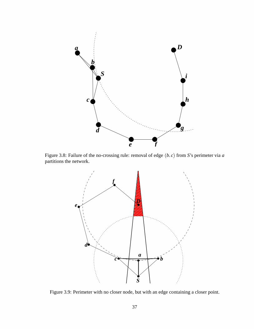
In Figure 3.8, we see an example of the first type, in which GPP’s no-crossing heuristic
ignores an edge that effectively partitions the network. Node S originates a packet toD,
35
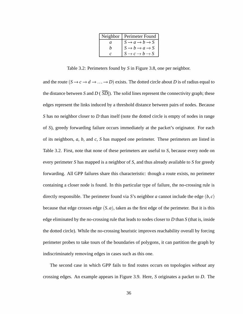
Neighbor Perimeter Founda S! a! b! Sb S! b! a! Sc S! c! b! S
Table 3.2: Perimeters found byS in Figure 3.8, one per neighbor.
and the route(S! c! d! : : :!D) exists. The dotted circle aboutD is of radius equal to
the distance betweenSandD (jSDj). The solid lines represent the connectivity graph; these
edges represent the links induced by a threshold distance between pairs of nodes. Because
Shas no neighbor closer toD than itself (note the dotted circle is empty of nodes in range
of S), greedy forwarding failure occurs immediately at the packet’s originator. For each
of its neighbors,a, b, andc, S has mapped one perimeter. These perimeters are listed in
Table 3.2. First, note that none of these perimeters are useful to S, because every node on
every perimeterShas mapped is a neighbor ofS, and thus already available toSfor greedy
forwarding. All GPP failures share this characteristic: though a route exists, no perimeter
containing a closer node is found. In this particular type offailure, the no-crossing rule is
directly responsible. The perimeter found viaS’s neighbora cannot include the edge(b;c)because that edge crosses edge(S;a), taken as the first edge of the perimeter. But it is this
edge eliminated by the no-crossing rule that leads to nodes closer toD thanS(that is, inside
the dotted circle). While the no-crossing heuristic improves reachability overall by forcing
perimeter probes to take tours of the boundaries of polygons, it can partition the graph by
indiscriminately removing edges in cases such as this one.
The second case in which GPP fails to find routes occurs on topologieswithout any
crossing edges. An example appears in Figure 3.9. Here,Soriginates a packet toD. The
36
Da
b
S
c
d
e f
h
g
i
Figure 3.8: Failure of the no-crossing rule: removal of edge(b;c) from S’s perimeter viaapartitions the network.
e
f
S
������������������������������
������������������������������
D
abc
d
Figure 3.9: Perimeter with no closer node, but with an edge containing a closer point.
37
Neighbor Perimeter FoundS a! S! c! ab a! b! S! ac a! c! b! a
Table 3.3: Perimeters found bya in Figure 3.9, one per neighbor.
path(S! c! d! e! f ! D) clearly exists. Initially,S forwards the packet greedily to
a. The dotted circle representsS’s radio range, and the dashed circle is the circle centered
atD with radiusjaDj, inside which nodes are closer toD thana. At a, greedy forwarding is
impossible (note the empty intersection of the dotted and dashed circles), buta has learned
no perimeter containing a node inside the dotted circle, andso GPP drops the packet for
D. The perimeters learned bya are shown in Table 3.3. Note that while the perimeter
learned bya via c, (a! c! b! a), includes edge(c;b), which includes points closer to
the destinationD. GPP only examines locations of nodes (vertices), not links(edges). In
fact, GPP will fail to forward any packet to a destination in the shaded region that reachesa
successfully. The two heavy lines, which are the perpendicular bisectors of edges(c;S) and(b;S), bound the regiona is closer to than bothc andb. Eliminating the portion ofa’s radio
range that overlaps this region leaves the shaded region. Both b andc will forward packets
bound for destinations in the shaded region toa greedily, althougha has no perimeter to
help it forward toward these destinations, and bothb andc do learn perimeters that will
help them forward toward these destinations.
38
3.3 Planarized Graphs
While measurements taken in simulations show that GPP with the no-crossing heuristic
finds the vast majority of routes (over 99.5% of then2 routes amongn nodes) in randomly
generated networks, it is unacceptable for a routing algorithm persistently to fail to find
a route to a reachable node in a static, unchanging network topology. Motivated by the
insufficiency of GPP’s no-crossing heuristic, we present alternative methods for eliminating
crossing links from the network.
A graph in which no two edges cross is known asplanar. As has been done in the
idealized simulations presented so far in this thesis, a setof nodes with radios, where all
radios have identical, circular radio ranger, can be seen as a graph: each node is a vertex,
and edge(n;m) exists between nodesn andm if the distance betweenn andm, d(n;m)�r. Graphs whose edges are dictated by a threshold distance between vertices are termed
unit graphs. In the sense that network radio hardware is traditionally viewed as having a
nominal open-space range (e.g., 250 meters for 900 MHz DSSS WaveLAN), this model is
reasonable. We additionally assume that the nodes in the network have negligible difference
in altitude, so that they can be considered roughly in a plane. We discuss these assumptions
further in Section 5.3.
The Relative Neighborhood Graph (RNG)and Gabriel Graph (GG)are two planar
graphs long-known in varied disciplines [12], [40]. An algorithm for removing edges from
the graph that are not part of the RNG or GG would yield a network with no crossing links.
For our application, the algorithm should be run in a distributed fashion by each node in the
network, where a node needs information only about the localtopology as the algorithm’s
39
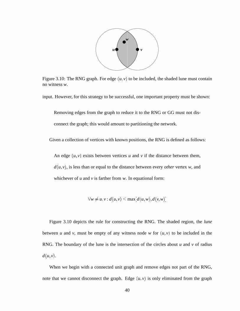
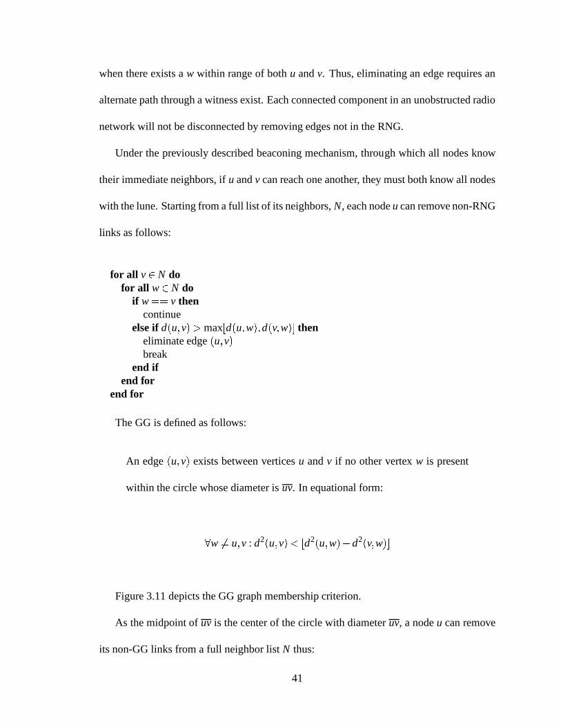
u v
w
Figure 3.10: The RNG graph. For edge(u;v) to be included, the shaded lune must containno witnessw.
input. However, for this strategy to be successful, one important property must be shown:
Removing edges from the graph to reduce it to the RNG or GG mustnot dis-
connect the graph; this would amount to partitioning the network.
Given a collection of vertices with known positions, the RNGis defined as follows:
An edge(u;v) exists between verticesu andv if the distance between them,
d(u;v), is less than or equal to the distance between everyothervertexw, and
whichever ofu andv is farther fromw. In equational form:8w 6= u;v : d(u;v)�max[d(u;w);d(v;w)℄Figure 3.10 depicts the rule for constructing the RNG. The shaded region, thelune
betweenu andv, must be empty of any witness nodew for (u;v) to be included in the
RNG. The boundary of the lune is the intersection of the circles aboutu andv of radius
d(u;v).When we begin with a connected unit graph and remove edges notpart of the RNG,
note that we cannot disconnect the graph. Edge(u;v) is only eliminated from the graph
40
when there exists aw within range of bothu andv. Thus, eliminating an edge requires an
alternate path through a witness exist. Each connected component in an unobstructed radio
network will not be disconnected by removing edges not in theRNG.
Under the previously described beaconing mechanism, through which all nodes know
their immediate neighbors, ifu andv can reach one another, they must both know all nodes
with the lune. Starting from a full list of its neighbors,N, each nodeu can remove non-RNG
links as follows:
for all v2 N dofor all w2 N do
if w== v thencontinue
else ifd(u;v)> max[d(u;w);d(v;w)℄ theneliminate edge(u;v)break
end ifend for
end for
The GG is defined as follows:
An edge(u;v) exists between verticesu andv if no other vertexw is present
within the circle whose diameter isuv. In equational form:
8w 6= u;v : d2(u;v)< [d2(u;w)+d2(v;w)℄Figure 3.11 depicts the GG graph membership criterion.
As the midpoint ofuv is the center of the circle with diameteruv, a nodeu can remove
its non-GG links from a full neighbor listN thus:
41
u v
w
Figure 3.11: The GG graph. For edge(u;v) to be included, the shaded circle must containno witnessw.
m = midpoint ofuvfor all v2 N do
for all w2 N doif w== v then
continueelse ifd(m;w)< d(u;m) then
eliminate edge(u;v)break
end ifend for
end for
Eliminating edges in the GG cannot disconnect a connected unit graph, for the same
reason as was the case for the RNG. Both these algorithms for rendering the graph of the
radio network planar take timeO(deg2) at each node, where deg is the node’s degree in the
full radio graph.
The RNG is a subset of the GG. This is consistent with the smaller shaded region
searched for a witness in the GG, as compared with in the RNG. Figure 3.12 shows a full
unit graph corresponding to 200 nodes randomly placed on a 2000-by-2000-meter region,
with radio ranges of 250 meters; the GG subset of the full graph; and the RNG subset of
the full graph. Note that the RNG and GG offer different densities of connectivity by elim-
inating different numbers of links. Many MAC layers exhibitdrastically reduced efficiency
42
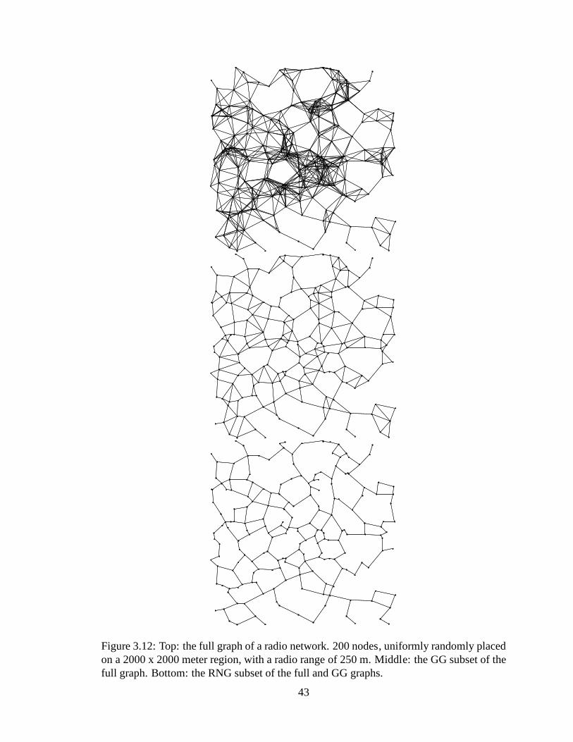
Figure 3.12: Top: the full graph of a radio network. 200 nodes, uniformly randomly placedon a 2000 x 2000 meter region, with a radio range of 250 m. Middle: the GG subset of thefull graph. Bottom: the RNG subset of the full and GG graphs.
43
as the number of mutually reachable sending stations increases [1], [8]. Moreover, while
any packet a node transmits monopolizes the shared channel within its radio range, MAC
protocols that address the hidden terminal problem, including 802.11 [17],MACA [21],
andMACAW [4], deliberately spread contention to the full radio ranges of bothsender and
receiver. On some Frequency Hopping Spread Spectrum MACs, such as Metricom’s [3],
collisions occur when more than one of a node’s neighbors send to it simultaneously. Un-
der such regimes, using fewer links in routing can alleviatecontention, and thus increase
efficiency.
3.4 GPSR: Combining Greedy and Planar Perimeters
We now present the full Greedy Perimeter Stateless Routing algorithm, which combines
greedy forwarding (Section 2.1) on the full network graph with perimeter forwarding on
the planarized network graph where greedy forwarding is notpossible [23]. Recall that all
nodes maintain a neighbor table, which stores the addressesand locations of their single-
hop radio neighbors. This table provides all state requiredfor GPSR’s forwarding deci-
sions, beyond the state in the packets themselves.
The packet header fields GPSR uses in perimeter-mode forwarding are shown in Ta-
ble 3.4. GPSR packet headers include a flag field indicating whether the packet is in
greedy mode or perimeter mode. All data packets are marked initially at their origina-
tors as greedy-mode. Packet sources also include the geographic location of the destination
in packets. Only a packet’s source sets the location destination field; it is left unchanged as
the packet is forwarded through the network.
44
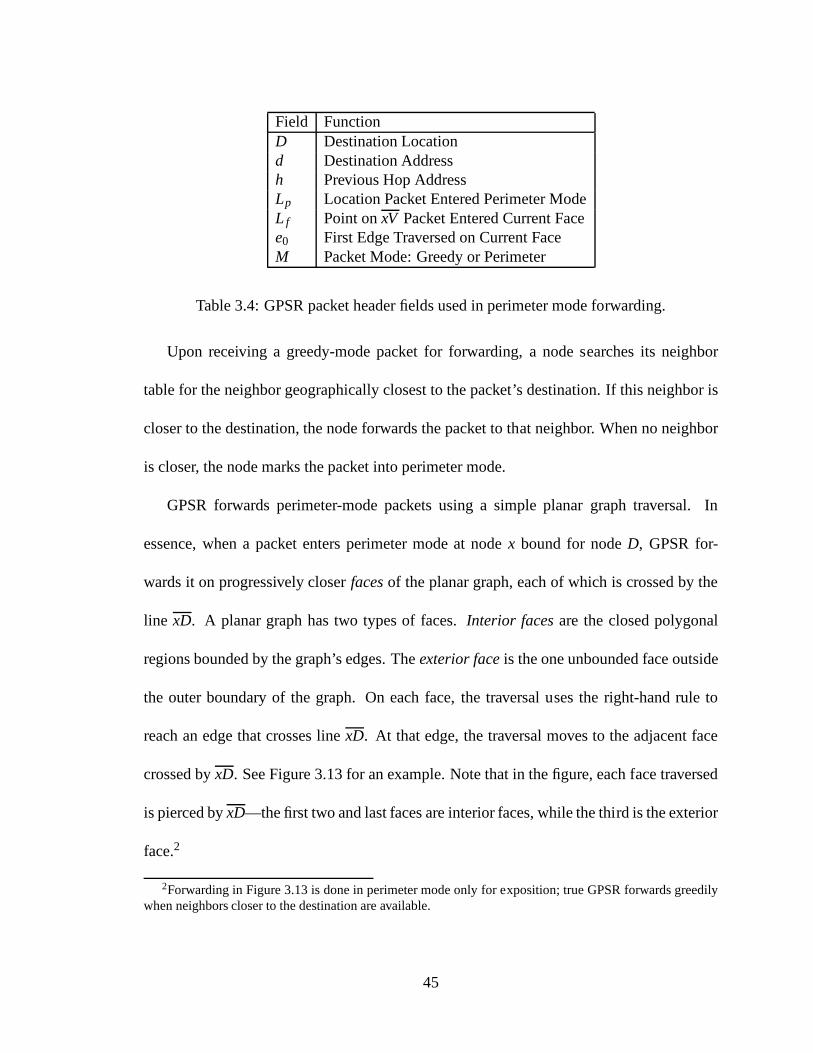
Field FunctionD Destination Locationd Destination Addressh Previous Hop AddressLp Location Packet Entered Perimeter ModeL f Point onxV Packet Entered Current Facee0 First Edge Traversed on Current FaceM Packet Mode: Greedy or Perimeter
Table 3.4: GPSR packet header fields used in perimeter mode forwarding.
Upon receiving a greedy-mode packet for forwarding, a node searches its neighbor
table for the neighbor geographically closest to the packet’s destination. If this neighbor is
closer to the destination, the node forwards the packet to that neighbor. When no neighbor
is closer, the node marks the packet into perimeter mode.
GPSR forwards perimeter-mode packets using a simple planargraph traversal. In
essence, when a packet enters perimeter mode at nodex bound for nodeD, GPSR for-
wards it on progressively closerfacesof the planar graph, each of which is crossed by the
line xD. A planar graph has two types of faces.Interior facesare the closed polygonal
regions bounded by the graph’s edges. Theexterior faceis the one unbounded face outside
the outer boundary of the graph. On each face, the traversal uses the right-hand rule to
reach an edge that crosses linexD. At that edge, the traversal moves to the adjacent face
crossed byxD. See Figure 3.13 for an example. Note that in the figure, each face traversed
is pierced byxD—the first two and last faces are interior faces, while the third is the exterior
face.2
2Forwarding in Figure 3.13 is done in perimeter mode only for exposition; true GPSR forwards greedilywhen neighbors closer to the destination are available.
45
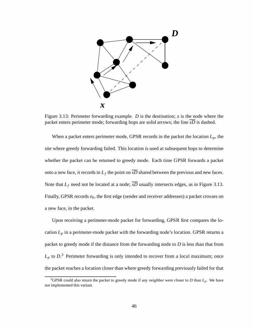
D
xFigure 3.13: Perimeter forwarding example.D is the destination;x is the node where thepacket enters perimeter mode; forwarding hops are solid arrows; the linexD is dashed.
When a packet enters perimeter mode, GPSR records in the packet the locationLp, the
site where greedy forwarding failed. This location is used at subsequent hops to determine
whether the packet can be returned to greedy mode. Each time GPSR forwards a packet
onto a new face, it records inL f the point onxD shared between the previous and new faces.
Note thatL f need not be located at a node;xD usually intersects edges, as in Figure 3.13.
Finally, GPSR recordse0, the first edge (sender and receiver addresses) a packet crosses on
a new face, in the packet.
Upon receiving a perimeter-mode packet for forwarding, GPSR first compares the lo-
cationLp in a perimeter-mode packet with the forwarding node’s location. GPSR returns a
packet to greedy mode if the distance from the forwarding node toD is less than that from
Lp to D.3 Perimeter forwarding is only intended to recover from a local maximum; once
the packet reaches a location closer than where greedy forwarding previously failed for that
3GPSR could also return the packet to greedy mode if anyneighborwere closer toD thanLp. We havenot implemented this variant.
46
packet, the packet can continue greedy progress toward the destination without danger of
returning to the prior local maximum.
When a packet enters perimeter mode atx, GPSR forwards it along the face intersected
by the linexD. Nodex forwards the packet to the first edge counterclockwise aboutx from
the linexD. This determines the first face over which to forward the packet. Thereafter,
GPSR forwards the packet around that face using the right-hand rule. There are two cases
to consider: eitherx andD are connected by the graph, or they are not.
When x andD are connected by the graph, traversing the face borderingx in either
direction (we use the previously described right-hand rule) must lead to a pointy at which
xD intersects the far side of the face. This is the case whether the traversed face is inte-
rior or exterior. Aty, GPSR has clearly reduced the distance between the packet and its
destination, in comparison with the packet’s start in perimeter mode atx.
While forwarding around a face, GPSR determines whether theedge to the chosen next
hopn intersectsxD. GPSR has the information required to make this determination, asLp
andD are recorded in the packet, and a GPSR node stores its own position and those of its
neighbors. If a node borders the edge where this intersection pointy lies, GPSR sets the
packet’sL f to y. At this point, the packet is forwarded along thenextface bordering point
y that is intersected byxD. The node forwards the packet along the first edge of this next
face—by the right-hand rule, the next edge counterclockwise about itself fromn. This first
edge on the new face is recorded in the packet’se0 field.
This process repeats at successively closer faces toD. At each face, the packet pro-
gresses by the right-hand rule until reaching the edge that interesects withxD at a pointy
47
closer than the packet’sL f field to D. Finally, the face containingD is reached, and the
right-hand-rule leads toD along that face.
WhenD is not reachable (i.e., it is disconnected from the graph), two cases exist: the
disconnected node lies either inside an interior face, or outside the exterior face. GPSR will
forward a perimeter-mode packet until the packet reaches the corresponding face. Upon
reaching this interior or exterior face, the packet will tour unsuccessfully around the entirety
of the face, without finding an edge intersectingxD at a point closer toD thanL f . When
the packet traverses the first edge it took on this face for thesecond time, GPSR notices
the repetition of forwarding on the edgee0 stored in the packet, and correctly drops the
packet, as the destination is unreachable; the perimeter-mode graph traversal to a reachable
destination never sends a packet across the same link in the same direction twice.
Figure 3.14 shows pseudocode for the GPSR forwarding algorithm. Note that we
assume throughout this pseudocode thatRIGHT-HAND-FORWARD, FACE-CHANGE, and
PERI-INIT-FORWARD operate on a pre-planarized graph, with crossing edges already re-
moved; we omit this detail in the pseudocode.GPSR-FORWARD is the top-level forwarding
function called for all arriving packets, with argumentsp, the packet being forwarded, and
nin, the neighbor from which the packet arrived.4 If p is a greedy data packet, and greedy
forwarding fails,GPSR-FORWARD sets the locations where the packet entered perimeter
mode (p:Lp) and where the line to the destination intersected the current face (p:L f ) to
the router’s own position.PERI-INIT-FORWARD finds the next routert counterclockwise
from the line to the destination, using the same algorithm asRIGHT-HAND-FORWARD. Fi-
4If the packet originated at the local node,nin is unused.
48
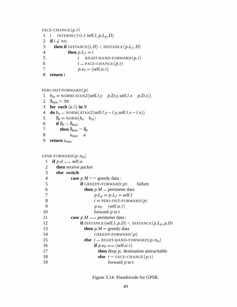
FACE-CHANGE(p; t)1 i = INTERSECT(t:l ;self:l ; p:Lp;D)2 if i 6= NIL
3 then if DISTANCE(i;D)< DISTANCE(p:L f ;D)4 then p:L f = i5 t = RIGHT-HAND-FORWARD(p; t)6 t = FACE-CHANGE(p; t)7 p:e0 = (self:a; t)8 return t
PERI-INIT-FORWARD(p)1 bin = NORM(ATAN 2(self:l :y� p:D:y;self:l :x� p:D:x))2 δmin = 3π3 for each (a; l) in N4 do ba = NORM(ATAN 2(self:l :y� l :y;self:l :x� l :x))5 δb = NORM(ba�bin)6 if δb < δmin7 then δmin = δb
8 amin = a9 return amin
GPSR-FORWARD(p;nin)1 if p:d == self:a2 then receive packet3 else switch4 casep:M == greedy data :5 if GREEDY-FORWARD(p) == failure6 then p:M = perimeter data7 p:Lp = p:L f = self:l8 t = PERI-INIT-FORWARD(p)9 p:e0 = (self:a; t)
10 forwardp to t11 casep:M == perimeter data :12 if DISTANCE(self:l ; p:D)< DISTANCE(p:Lp; p:D)13 then p:M = greedy data14 GREEDY-FORWARD(p)15 else t = RIGHT-HAND-FORWARD(p;nin)16 if p:e0 == (self:a; t)17 then drop p; destination unreachable18 else t = FACE-CHANGE(p; t)19 forwardp to t
Figure 3.14: Pseudocode for GPSR.
49
nally, GPSR-FORWARD sets the first edge taken on the perimeter in the packet (p:e0), and
forwards the packet tot.
Upon receiving a perimeter-mode packet,GPSR-FORWARD first determines whether the
packet has reached a node closer to the destination than the point where it entered perimeter
mode; if so, it returns the packet to greedy mode, and forwards it greedily. Otherwise,
GPSR-FORWARD calls RIGHT-HAND-FORWARD to determine the next hop router dictated
by the right-hand rule. If this next edge is the same as the first edge the packet traversed
on the current face (p:e0), the packet has toured the entire face, and the destinationis
unreachable, so the packet is dropped. If the packet hasn’t toured the entire face,GPSR-
FORWARD calls FACE-CHANGE to determine whether the packet has reached an edge that
crosses the line to the destination.FACE-CHANGE returns the appropriate next hop for the
first edge on the next face if such a crossing edge has been reached, or the unchanged next
hop found by the right-hand rule if no crossing of the line to the destination is found. Note
that changing faces amounts to treating the next hop on the current face as theprevious
hop, and applying the right-hand rule.FACE-CHANGE calls itself recursively, because it
is possible that a single node bordersmultipleedges that cross the line to the destination.
The recursion terminates upon reaching the edge that crosses the line at theclosestpoint to
the destination; it must terminate because there is always an edge that crosses the line at a
point farther than this closest point.
GPSR will greedily forward a packet to an unreachable destination for potentially many
hops before the packet loops on an exterior or interior face and is recognized as undeliver-
able. If the majority of unreachable destinations lie beyond the boundary of a single face,
50
undeliverable packets may concentrate at that face of the network graph. This behavior is
a direct consequence of GPSR’s avoidance of transitive routing protocol traffic across the
many hops from a destination to a forwarding router. Other techniques for scaling routing
have similar effects, however: the hierarchy used to scale routing on wired networks ob-
scures intra-domain link failures from the backbone in the interest of scaling. Thus, the
inter-domain routing system will push a packet a great distance, with the potential result
that the packet will be dropped inside the destination AS.
By the end-to-end argument [36], the most logical place for routing unreachability to
be determined, and the load on the network from undeliverable packets to be reduced, is at
the sending end-system. Mechanisms from inside the network, like ICMP Unreachable, are
hard to interpret at senders; it is hard to know on what timescale they indicate unreachabil-
ity, for example. Applications running over a GPSR-routed network, or any other network,
should offer a conforming load; senders should cut their transmission rate absent feedback
from receivers.
On a static network, GPSR finds all existing routes (that is, on network graphs where
the destination is connected). This fact is clear by inspection: greedy forwarding moves a
packet closer to the destination at each hop. Between when a packet enters perimeter mode
and leaves perimeter mode, the packet similarlymustmove closer to the destination. If the
packet reaches the destination while still in perimeter mode, GPSR clearly finds the route.
GPSR only returns a packet to greedy mode from perimeter modewhen the packet reaches
a point closer to the destination than that where it entered perimeter mode,Lp. If there
exists a path to the destination, then the line from the pointof entry to perimeter mode to
51
the destinationmustcut a sequence of adjacent faces on the planarized graph. Theright-
hand rule visits all edges on a face, until reaching the destination if it is on that face, or the
border of the next face cut by the line betweenLp and the destination.
Moreover, GPSR never causes a packet to loop forever on a static network. Greedy
mode cannot cause a packet to loop, because each greedy hop must move the packet strictly
closer to the destination. As stated just above, GPSR never returns a packet to greedy mode
from perimeter mode unless the packet has reached a point closer than that where it entered
perimeter mode. What remains to be shown is that an invocation of perimeter mode does
not loop a packet forever. Perimeter mode traverses a seriesof adjacent faces, each by the
right-hand rule. Because the graph is planar, traversal of aface by the right-hand rulemust
visit each edge on the face. If the destination is connected,theremustexist a sequence
of adjacent faces along the line betweenLp and the destination, and the right-hand rule
mustvisit the border edge between each pair of these adjacent faces. If the destination is
disconnected, then GPSR drops the packet when it visits the first edge taken on a face (e0)
for the second time. Thus, GPSR never loops packets on staticnetworks.
3.5 Robustness and Efficiency on Mobile Networks
To make GPSR robust and efficient on a mobile, wireless IEEE 802.11 network, we made
several significant design decisions in and embellishmentsto the GPSR algorithm.
52

3.5.1 Use of MAC-Layer Failure Feedback
As done in DSR [7], GPSR receives notification from the 802.11MAC layer when a
packet exceeds its maximum number of retransmit retries. Barring congestive collapse, a
retransmit-retry-exceeded failure indicates that the intended recipient has left radio range,
either because the recipient failed, or because of motion ofthe recipient and/or sender.
GPSR responds to these notifications by eliminating the destination of the failed packet
from its neighbor table. The data packet that elicits such a notification is passed back to
the GPSR forwarding logic, for re-forwarding using the newly reduced neighbor table. Use
of this feedback often informs GPSR far earlier than otherwise possible through expiration
of the neighbor timeout interval (4:5B). This technique allows GPSR nodes to keep more
accurate neighbor tables, and therefore make forwarding decisions that more often reflect
the current local topology, rather than a stale version of the local topology.
3.5.2 Interface Queue Traversal
Related to MAC-layer feedback, this technique has a profound effect on our results. While
an IEEE 802.11 interface repeatedly retransmits the packetat the head of its queue, backing
off exponentially between retransmit attempts, it head-of-line blocks, waiting for a link-
level acknowledgement from the receiver. This head-of-line blocking reduces the available
transmit duty cycle of the interface significantly. For thisreason, upon notification of a
MAC retransmit retry failure, we traverse the queue of packets for the interface, and re-
move all packets addressed to the failed transmission’s recipient. We pass these packets
back to the routing protocol for re-forwarding to a different next hop. This change virtually
53
eliminated what we’d previously thought to be MAC contention in high-mobility simula-
tions where neighbors were lost frequently; the timeouts and head-of-line blocking were
what really had been causing the drops at the interface queue. The implementation of DSR
for ns-2 [38] implements this useful optimization, though we don’t see it mentioned in the
published work on DSR.
3.5.3 Promiscuous Use of the Network Interface
Also as used in DSR [7], GPSR disables MAC address filtering onthe IEEE 802.11 ra-
dio hardware to receive copies of all packets for all stations within its radio range. As
described in Section 2.1, all packets carry their local sender’s position, to reduce the rate
at which beacon packets must be sent, and to keep positions inneighbor lists maximally
current in regions under data traffic load. When a node forwards a data packet, it resets the
timer for transmitting the next beacon, since data packets carry beacon-equivalent (address,
position) reports. While this technique lengthens data packets by twelve bytes, on shared-
medium wireless MACs that use collision avoidance, including IEEE 802.11, the overhead
of acquiring the channel for transmitting a packet is much larger than that of lengthening a
packet by a dozen bytes. Thus, this optimization also results in use of less of the channel ca-
pacity. There is, of course, a power cost in running the IEEE 802.11 radio receive hardware
for all packets, regardless of their destination address. But IEEE 802.11 radio hardware im-
plementations expend significantly less power while receiving packets than they do while
transmitting packets. We have not performed power consumption measurements of GPSR.
54
3.5.4 Planarization Triggers
Both the RNG and GG planarizations depend on having current position information for
a node’s current set of neighbors. We have implemented both planarizations, though the
results we present in this thesis use only the RNG. As nodes move, a planarization becomes
stale, and less useful for accurate perimeter-mode packet forwarding. In our current imple-
mentation, we re-planarize the graph upon every acquisition of a new neighbor, and every
loss of a former neighbor, as distinguishable by receipt of abeacon or data packet (promis-
cuously) from a previously unknown neighbor, and by a beacontimeout for a neighbor,
or MAC transmit failure indication. However, this choice will not keep the planarization
current if nodes only movewithin a node’s radio range, but no nodes move into or out of
it. In future, we will incrementally update the planarization upon receipt of every beacon
(or promiscuous data packet) from a neighbor, to keep the planarized graph maximally
up-to-date.
55
Chapter 4
Simulation Results and Evaluation
To measure our success in meeting the design goals for GPSR, we simulate the algorithm
on a variety of static and mobile network topologies [23]. Wefocus mainly on the mobile
simulation results in this thesis, as that part of the designspace is more demanding of a
routing protocol—link additions and removals are far more frequent under mobility. To
compare the performance of GPSR with prior work in wireless routing, we also simulate
Johnsonet al.’s Dynamic Source Routing, DSR [18], [27], which has been shown to offer
higher packet delivery ratios and lower routing protocol overhead than several other ad-hoc
routing protocols [7].
4.1 Simulation Environment
We simulated GPSR in ns-2 [39], using the wireless extensions developed at Carnegie
Mellon [38]. This simulation environment offers high fidelity, as it includes full simulation
of the IEEE 802.11 physical and MAC layers. Moreover, by using the same simulation
56
code base as the measurement study used to evaluate DSR [7], we ensure our results are
directly comparable to those published previously.
The ns-2 wireless simulation model simulates nodes moving in an unobstructed plane.
Motion follows therandom waypointmodel [7]: a node chooses a destination uniformly
at random in the simulated region, chooses a velocity uniformly at random from a config-
urable range, and then moves to that destination at the chosen velocity. Upon arriving at the
chosen waypoint, the node pauses for a configurable period before repeating the same pro-
cess. In this model, the pause time acts as a proxy for the degree of mobility in a simulation;
longer pause time amounts to more nodes being stationary formore of the simulation.
Our simulations are for networks of 50, 112, and 200 nodes with 802.11 WaveLAN
radios, with a nominal 250-meter range. In the simulations where we compare GPSR with
DSR, we use simulation parameters identical to a subset of those used by Brochet al. [7];
only the number of nodes, in the case of the 112- and 200-node simulations, differs. The
nodes are initially placed uniformly at random in a rectangular region. All nodes move
according to the random waypoint model, with a velocity chosen uniformly in[1;20℄ m/s.
We simulate pause times of 0, 30, 60, and 120 seconds, the highest mobility cases, as they
are the most demanding of a routing algorithm. Brochat al. also simulated 300-, 600-,
and 900-second pause times, perhaps in large part because two of the routing algorithms
they evaluated (DSDV and TORA) performed well in these cases. We simulate 30 CBR
traffic flows, originated by 22 sending nodes. Each CBR flow sends at 2 Kbps, and uses
64-byte packets. The flows are low-bitrate because the IEEE 802.11 MAC is prone to
congestion, and these simulations are meant to measure routing protocol behavior, not the
57
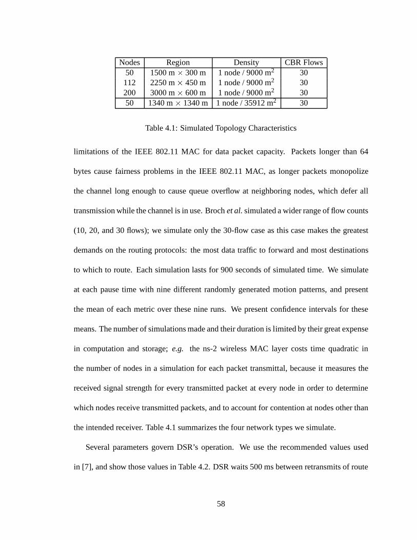
Nodes Region Density CBR Flows50 1500 m� 300 m 1 node / 9000 m2 30112 2250 m� 450 m 1 node / 9000 m2 30200 3000 m� 600 m 1 node / 9000 m2 3050 1340 m� 1340 m 1 node / 35912 m2 30
Table 4.1: Simulated Topology Characteristics
limitations of the IEEE 802.11 MAC for data packet capacity.Packets longer than 64
bytes cause fairness problems in the IEEE 802.11 MAC, as longer packets monopolize
the channel long enough to cause queue overflow at neighboring nodes, which defer all
transmission while the channel is in use. Brochet al.simulated a wider range of flow counts
(10, 20, and 30 flows); we simulate only the 30-flow case as thiscase makes the greatest
demands on the routing protocols: the most data traffic to forward and most destinations
to which to route. Each simulation lasts for 900 seconds of simulated time. We simulate
at each pause time with nine different randomly generated motion patterns, and present
the mean of each metric over these nine runs. We present confidence intervals for these
means. The number of simulations made and their duration is limited by their great expense
in computation and storage;e.g. the ns-2 wireless MAC layer costs time quadratic in
the number of nodes in a simulation for each packet transmittal, because it measures the
received signal strength for every transmitted packet at every node in order to determine
which nodes receive transmitted packets, and to account forcontention at nodes other than
the intended receiver. Table 4.1 summarizes the four network types we simulate.
Several parameters govern DSR’s operation. We use the recommended values used
in [7], and show those values in Table 4.2. DSR waits 500 ms between retransmits of route
58
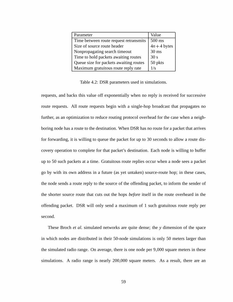
Parameter ValueTime between route request retransmits500 msSize of source route header 4n+4 bytesNonpropagating search timeout 30 msTime to hold packets awaiting routes 30 sQueue size for packets awaiting routes50 pktsMaximum gratuitous route reply rate 1/s
Table 4.2: DSR parameters used in simulations.
requests, and backs this value off exponentially when no reply is received for successive
route requests. All route requests begin with a single-hop broadcast that propagates no
further, as an optimization to reduce routing protocol overhead for the case when a neigh-
boring node has a route to the destination. When DSR has no route for a packet that arrives
for forwarding, it is willing to queue the packet for up to 30 seconds to allow a route dis-
covery operation to complete for that packet’s destination. Each node is willing to buffer
up to 50 such packets at a time. Gratuitous route replies occur when a node sees a packet
go by with its own address in a future (as yet untaken) source-route hop; in these cases,
the node sends a route reply to the source of the offending packet, to inform the sender of
the shorter source route that cuts out the hopsbeforeitself in the route overheard in the
offending packet. DSR will only send a maximum of 1 such gratuitous route reply per
second.
These Brochet al. simulated networks are quite dense; they dimension of the space
in which nodes are distributed in their 50-node simulationsis only 50 meters larger than
the simulated radio range. On average, there is one node per 9,000 square meters in these
simulations. A radio range is nearly 200,000 square meters.As a result, there are an
59
average of approximately 20 neighbors within range of the average node in these networks.
DSR’s caching of overheard routes gives great benefit in suchdense topologies. And GPSR
can use greedy mode to forward the vast majority of packets.
The last line in Table 4.1 shows a much sparser network configuration that we simulate.
In these simulations, the node density is one quarter that inthe Broch simulations, and we
use a region with a square aspect ratio. The purpose of this last group of measurements is to
evaluate the effect of node density on GPSR’s performance; recall that greedy forwarding
is used less frequently on sparser networks, as shown in Section 2.5.
Our simulations do not include a distributed location database for annotating packets
with destinations’ positions. Our results here argue that the GPSR approach to routing
warrants investigation into efficient location databases,and related work is already under-
way in this area [25]. In these simulation results, we use an idealized location database:
each source annotates packets it originates with the true location of the destination. In this
sense, our results represent the lowest control packet loadthat can be expected from GPSR.
Section 5.2 discusses GPSR’s interaction with a location database further.
Before gathering the measurement results we present here, we validated the GPSR im-
plementation extensively by running it on hundreds ofnon-mobiletopologies, over an ideal
MAC layer (the Null MAC [38]), a 2 Mbps, contention-free network. Our goal in these
tests is to achieve 100% delivery success to demonstrate that the GPSR code makes correct
forwarding decisions. After reaching this 100% goal on the Null MAC, we validated the
GPSR implementation on these non-mobile topologies atop the ns 802.11 MAC layer, to
verify GPSR’s response to MAC transmit failure callbacks.
60
We evaluate GPSR and DSR using four metrics: packet deliverysuccess rate, routing
protocol overhead, optimality of path lengths taken by datapackets, and state per router.
The first measurements we present are for 50-node topologiesand mobility characteris-
tics identical to those simulated in [7], for clearest comparison with prior published results
on DSR. Thereafter, we present and discuss measurements on networks with 112 and 200
nodes, and reveal the scaling properties of GPSR and DSR as network diameter increases.
Next, we investigate the effect of node density on GPSR’s performance. Finally, we con-
clude with measurements of the state used on average in each router by GPSR and DSR.
4.2 Packet Delivery Success Rate
Figure 4.1 shows how many application packets GPSR deliverssuccessfully for varying
values ofB, the beaconing interval, as a function of pause time. The same figure for DSR is
included for comparison. All data points are bracketed by their 97.7% confidence interval.1
Note the narrow range of values on they axis; all algorithms on this graph deliver over
97% of user packets on average. Only packets for which a pathexiststo the destination are
included in the graph; delivery failure to a truly disconnected destination does not represent
failure of a routing algorithm. However, as mentioned above, disconnection of a node is
extremely rare in these simulations, as connectivity is dense. As one would expect, the
decrease in precision of neighbor lists caused by the longerbeaconing interval of 3 seconds
results in a slightly reduced delivery success rate. But it appears that there is little added
1The use of 97.7% as the confidence interval is purely to allow use of 2, an easily remembered integer, asthe quantile of the unit normal distribution in the confidence interval calculation.
61
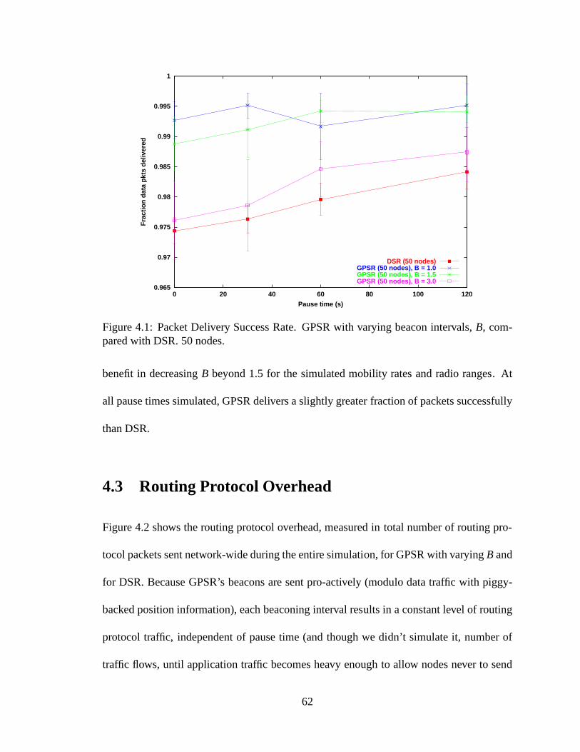
0.965
0.97
0.975
0.98
0.985
0.99
0.995
1
0 20 40 60 80 100 120
Fra
ctio
n d
ata
pkt
s d
eliv
ered
Pause time (s)
DSR (50 nodes)GPSR (50 nodes), B = 1.0GPSR (50 nodes), B = 1.5GPSR (50 nodes), B = 3.0
Figure 4.1: Packet Delivery Success Rate. GPSR with varyingbeacon intervals,B, com-pared with DSR. 50 nodes.
benefit in decreasingB beyond 1.5 for the simulated mobility rates and radio ranges. At
all pause times simulated, GPSR delivers a slightly greaterfraction of packets successfully
than DSR.
4.3 Routing Protocol Overhead
Figure 4.2 shows the routing protocol overhead, measured intotal number of routing pro-
tocol packets sent network-wide during the entire simulation, for GPSR with varyingB and
for DSR. Because GPSR’s beacons are sent pro-actively (modulo data traffic with piggy-
backed position information), each beaconing interval results in a constant level of routing
protocol traffic, independent of pause time (and though we didn’t simulate it, number of
traffic flows, until application traffic becomes heavy enoughto allow nodes never to send
62
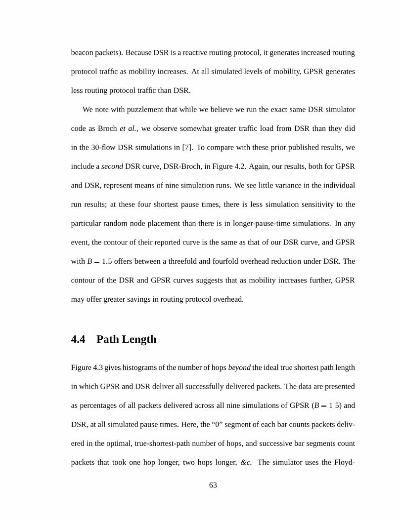
beacon packets). Because DSR is a reactive routing protocol, it generates increased routing
protocol traffic as mobility increases. At all simulated levels of mobility, GPSR generates
less routing protocol traffic than DSR.
We note with puzzlement that while we believe we run the exactsame DSR simulator
code as Brochet al., we observe somewhat greater traffic load from DSR than they did
in the 30-flow DSR simulations in [7]. To compare with these prior published results, we
include asecondDSR curve, DSR-Broch, in Figure 4.2. Again, our results, both for GPSR
and DSR, represent means of nine simulation runs. We see little variance in the individual
run results; at these four shortest pause times, there is less simulation sensitivity to the
particular random node placement than there is in longer-pause-time simulations. In any
event, the contour of their reported curve is the same as thatof our DSR curve, and GPSR
with B= 1:5 offers between a threefold and fourfold overhead reduction under DSR. The
contour of the DSR and GPSR curves suggests that as mobility increases further, GPSR
may offer greater savings in routing protocol overhead.
4.4 Path Length
Figure 4.3 gives histograms of the number of hopsbeyondthe ideal true shortest path length
in which GPSR and DSR deliver all successfully delivered packets. The data are presented
as percentages of all packets delivered across all nine simulations of GPSR (B= 1:5) and
DSR, at all simulated pause times. Here, the “0” segment of each bar counts packets deliv-
ered in the optimal, true-shortest-path number of hops, andsuccessive bar segments count
packets that took one hop longer, two hops longer,&c. The simulator uses the Floyd-
63
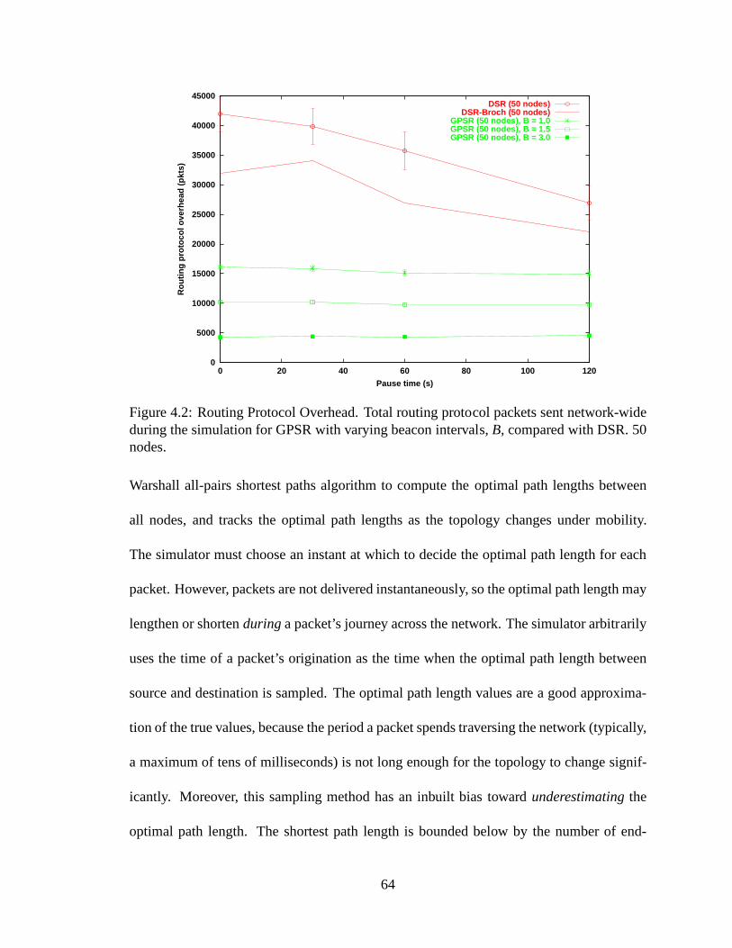
0
5000
10000
15000
20000
25000
30000
35000
40000
45000
0 20 40 60 80 100 120
Ro
uti
ng
pro
toco
l ove
rhea
d (
pkt
s)
Pause time (s)
DSR (50 nodes)DSR-Broch (50 nodes)
GPSR (50 nodes), B = 1.0GPSR (50 nodes), B = 1.5GPSR (50 nodes), B = 3.0
Figure 4.2: Routing Protocol Overhead. Total routing protocol packets sent network-wideduring the simulation for GPSR with varying beacon intervals,B, compared with DSR. 50nodes.
Warshall all-pairs shortest paths algorithm to compute theoptimal path lengths between
all nodes, and tracks the optimal path lengths as the topology changes under mobility.
The simulator must choose an instant at which to decide the optimal path length for each
packet. However, packets are not delivered instantaneously, so the optimal path length may
lengthen or shortenduringa packet’s journey across the network. The simulator arbitrarily
uses the time of a packet’s origination as the time when the optimal path length between
source and destination is sampled. The optimal path length values are a good approxima-
tion of the true values, because the period a packet spends traversing the network (typically,
a maximum of tens of milliseconds) is not long enough for the topology to change signif-
icantly. Moreover, this sampling method has an inbuilt biastowardunderestimatingthe
optimal path length. The shortest path length is bounded below by the number of end-
64
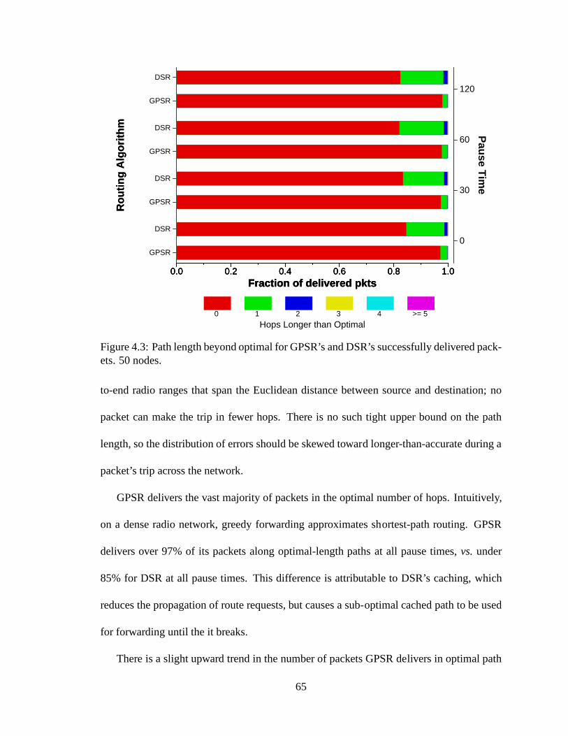
0.0 0.2 0.4 0.6 0.8 1.0Fraction of delivered pkts
GPSR
DSR
GPSR
DSR
GPSR
DSR
GPSR
DSR
0.0 0.2 0.4 0.6 0.8 1.0Fraction of delivered pkts
0
30
60
120P
ause T
ime
0.0 0.2 0.4 0.6 0.8 1.0Fraction of delivered pkts
Ro
uti
ng
Alg
ori
thm
Hops Longer than Optimal
Ro
uti
ng
Alg
ori
thm
0 1 2 3 4 >= 5
Figure 4.3: Path length beyond optimal for GPSR’s and DSR’s successfully delivered pack-ets. 50 nodes.
to-end radio ranges that span the Euclidean distance between source and destination; no
packet can make the trip in fewer hops. There is no such tight upper bound on the path
length, so the distribution of errors should be skewed toward longer-than-accurate during a
packet’s trip across the network.
GPSR delivers the vast majority of packets in the optimal number of hops. Intuitively,
on a dense radio network, greedy forwarding approximates shortest-path routing. GPSR
delivers over 97% of its packets along optimal-length pathsat all pause times,vs.under
85% for DSR at all pause times. This difference is attributable to DSR’s caching, which
reduces the propagation of route requests, but causes a sub-optimal cached path to be used
for forwarding until the it breaks.
There is a slight upward trend in the number of packets GPSR delivers in optimal path
65
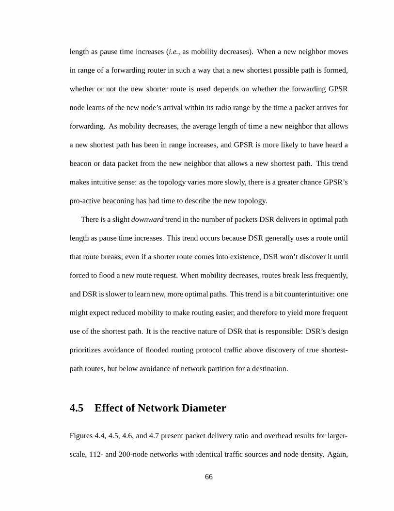
length as pause time increases (i.e., as mobility decreases). When a new neighbor moves
in range of a forwarding router in such a way that a new shortest possible path is formed,
whether or not the new shorter route is used depends on whether the forwarding GPSR
node learns of the new node’s arrival within its radio range by the time a packet arrives for
forwarding. As mobility decreases, the average length of time a new neighbor that allows
a new shortest path has been in range increases, and GPSR is more likely to have heard a
beacon or data packet from the new neighbor that allows a new shortest path. This trend
makes intuitive sense: as the topology varies more slowly, there is a greater chance GPSR’s
pro-active beaconing has had time to describe the new topology.
There is a slightdownwardtrend in the number of packets DSR delivers in optimal path
length as pause time increases. This trend occurs because DSR generally uses a route until
that route breaks; even if a shorter route comes into existence, DSR won’t discover it until
forced to flood a new route request. When mobility decreases,routes break less frequently,
and DSR is slower to learn new, more optimal paths. This trendis a bit counterintuitive: one
might expect reduced mobility to make routing easier, and therefore to yield more frequent
use of the shortest path. It is the reactive nature of DSR thatis responsible: DSR’s design
prioritizes avoidance of flooded routing protocol traffic above discovery of true shortest-
path routes, but below avoidance of network partition for a destination.
4.5 Effect of Network Diameter
Figures 4.4, 4.5, 4.6, and 4.7 present packet delivery ratioand overhead results for larger-
scale, 112- and 200-node networks with identical traffic sources and node density. Again,
66
all results represent the mean and 97.7% confidence intervals across 9 simulations. In these
measurements, the regions on which nodes move are 2250 by 450meters and 3000 by
600 meters, respectively, such that the number of square meters per node (9000 m2/node)
remains the same as that in the 50-node simulations. The intent in these simulations is to
evaluate the scaling of DSR and GPSR as network diameter increases. When routes are
longer, the probability of a route’s breaking increases. The traffic sources are the same as
in the smaller network simulations: 30 CBR sources of 2 Kbps each, transmitting 64-byte
packets. We do not increase the number of flows despite the increased number of nodes
in the network because DSR generates routing protocol packets reactively, and we seek to
measure DSR’s behavioronly on networks of wider diameter, not under workloads with
more destinations.
Note that in Figure 4.7, they axis is log-scaled. For each number of nodes, GPSR’s
traffic overhead once again remains flat, as it is a non-reactive protocol. At a constant
node density, network diameter has no effect on GPSR’slocal routing protocol message
traffic, since GPSR never sends routing packets beyond a single hop. This particular met-
ric, network-widecount of routing protocol packets, shows the GPSR beacon traffic to be
linear in node count, as compared with the 50-node simulations. DSR’s traffic overhead
is significantly larger on the wider-diameter, 112- and 200-node networks, as the protocol
must propagate source route information along the full length of a route, and longer routes
break more frequently. DSR’s caching of routes does not avoid this significant message
complexity increase. Note that comparing total numbers of routing protocol packets across
the entire network for varying number of nodes unfairly penalizes GPSR, in the sense that
67
GPSR generates a uniform routing protocol traffic distribution across nodes, because it is
purely pro-active and generates beacons at a fixed rate (modulo piggybacked position in-
formation on data packets). Because wireless network capacity increases with the spatial
diversity of transmitters, GPSR’s beacons offer the samelocal network load so long as
thedensityof nodes remains fixed. In contrast, DSR’s routing protocol overhead is decid-
edly non-linear in the number of nodes, such that the local network load caused by routing
protocol packets clearly increases significantly in the number of nodes.
GPSR’s traffic delivery ratio remains high at all pause timeson these larger-scale net-
works. It is GPSR’s use of only local topology information that allows the protocol to
maintain this delivery ratio; there is little penalty for GPSR as the path length from source
to destination lengthens. Moreover, GPSR recovers from loss of a neighbor by greedily
forwarding to another appropriate neighbor; this failoveris instantaneous. DSR’s delivery
ratio decreases considerably in the wider-diameter network, owing to DSR’s need to main-
tain full, end-to-end source routes, and re-query them increasingly frequently as diameter
and mobility increase.
Note that the maximum shortest path lengths between nodes inthese wider-diameter
simulations are still under 16 nodes. We mention this fact asthe DSR simulator code uses
a compile-time constant for the maximum length of a route it will discover, and maximum
propagation distance for route requests.
In these 112- and 200-node runs, DSR’s 64-route cache is fullat virtually every node.
While the number of destinations in the network is only 30 in our simulations, DSR caches
multiple routes per destination, and might profit from beingable to cache more routes,
68
0.8
0.82
0.84
0.86
0.88
0.9
0.92
0.94
0.96
0.98
1
0 20 40 60 80 100 120
Fra
ctio
n d
ata
pkt
s d
eliv
ered
Pause time (s)
DSR (112 nodes)GPSR (112 nodes), B = 1.5
Figure 4.4: Packet Delivery Success Rate. For GPSR withB = 1:5 compared with DSR.112 nodes.
though at the expense of increased per-router state (see thenext section).
Figures 4.8 and 4.9 show path length histograms for 112- and 200-node networks across
all pause times for DSR and GPSR, as presented before for 50-node networks. Here again,
as was the case in the 50-node path length data, GPSR consistently finds shorter paths
for a greater fraction of packets than DSR. However, as the network diameter increases,
both GPSR and DSR deliver fewer packets in the optimal path length. In the case of
GPSR, the longer the shortest path between two nodes, the greater the chance that the path
includes a node which has just arrived in range of its predecessor, and isn’t yet known to
the predecessor at the time the packet reaches the predecessor, resulting in a longer-than-
optimal path.2 Similarly, the longer a path between two nodes is, the greater the chance
2Of course, GPSR will always learn if the shortest path has become longer, because this situation cor-responds to loss of a neighbor, which will be indicated by a MAC layer retransmission retry failure for thatneighbor.
69
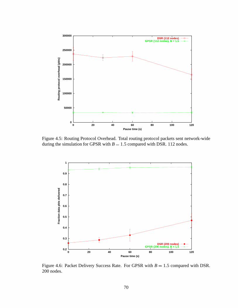
0
50000
100000
150000
200000
250000
300000
0 20 40 60 80 100 120
Ro
uti
ng
pro
toco
l ove
rhea
d (
pkt
s)
Pause time (s)
DSR (112 nodes)GPSR (112 nodes), B = 1.5
Figure 4.5: Routing Protocol Overhead. Total routing protocol packets sent network-wideduring the simulation for GPSR withB= 1:5 compared with DSR. 112 nodes.
0.2
0.3
0.4
0.5
0.6
0.7
0.8
0.9
1
0 20 40 60 80 100 120
Fra
ctio
n d
ata
pkt
s d
eliv
ered
Pause time (s)
DSR (200 nodes)GPSR (200 nodes), B = 1.5
Figure 4.6: Packet Delivery Success Rate. For GPSR withB = 1:5 compared with DSR.200 nodes.
70
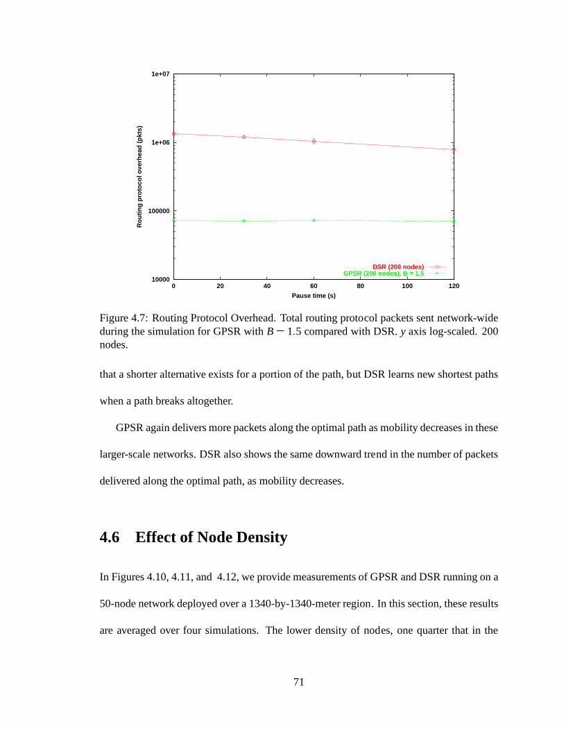
10000
100000
1e+06
1e+07
0 20 40 60 80 100 120
Ro
uti
ng
pro
toco
l ove
rhea
d (
pkt
s)
Pause time (s)
DSR (200 nodes)GPSR (200 nodes), B = 1.5
Figure 4.7: Routing Protocol Overhead. Total routing protocol packets sent network-wideduring the simulation for GPSR withB= 1:5 compared with DSR.y axis log-scaled. 200nodes.
that a shorter alternative exists for a portion of the path, but DSR learns new shortest paths
when a path breaks altogether.
GPSR again delivers more packets along the optimal path as mobility decreases in these
larger-scale networks. DSR also shows the same downward trend in the number of packets
delivered along the optimal path, as mobility decreases.
4.6 Effect of Node Density
In Figures 4.10, 4.11, and 4.12, we provide measurements of GPSR and DSR running on a
50-node network deployed over a 1340-by-1340-meter region. In this section, these results
are averaged over four simulations. The lower density of nodes, one quarter that in the
71

0.0 0.2 0.4 0.6 0.8 1.0Fraction of delivered pkts
GPSR
DSR
GPSR
DSR
GPSR
DSR
GPSR
DSR
0.0 0.2 0.4 0.6 0.8 1.0Fraction of delivered pkts
0
30
60
120
Pau
se Tim
e
0.0 0.2 0.4 0.6 0.8 1.0Fraction of delivered pkts
Ro
uti
ng
Alg
ori
thm
Hops Longer than Optimal
Ro
uti
ng
Alg
ori
thm
0 1 2 3 4 >= 5
Figure 4.8: Path length beyond optimal for GPSR’s and DSR’s successfully delivered pack-ets. 112 nodes.
72

0.0 0.2 0.4 0.6 0.8 1.0Fraction of delivered pkts
GPSR
DSR
GPSR
DSR
GPSR
DSR
GPSR
DSR
0.0 0.2 0.4 0.6 0.8 1.0Fraction of delivered pkts
0
30
60
120
Pau
se Tim
e
0.0 0.2 0.4 0.6 0.8 1.0Fraction of delivered pkts
Ro
uti
ng
Alg
ori
thm
Hops Longer than Optimal
Ro
uti
ng
Alg
ori
thm
0 1 2 3 4 >= 5
Figure 4.9: Path length beyond optimal for GPSR’s and DSR’s successfully delivered pack-ets. 200 nodes.
73
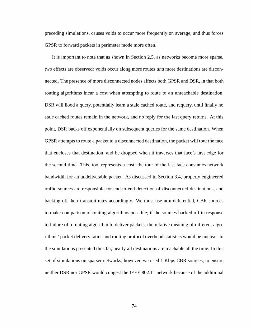
preceding simulations, causes voids to occur more frequently on average, and thus forces
GPSR to forward packets in perimeter mode more often.
It is important to note that as shown in Section 2.5, as networks become more sparse,
two effects are observed: voids occur along more routesandmore destinations are discon-
nected. The presence of more disconnected nodes affects both GPSR and DSR, in that both
routing algorithms incur a cost when attempting to route to an unreachable destination.
DSR will flood a query, potentially learn a stale cached route, and requery, until finally no
stale cached routes remain in the network, and no reply for the last query returns. At this
point, DSR backs off exponentially on subsequent queries for the same destination. When
GPSR attempts to route a packet to a disconnected destination, the packet will tour the face
that encloses that destination, and be dropped when it traverses that face’s first edge for
the second time. This, too, represents a cost; the tour of thelast face consumes network
bandwidth for an undeliverable packet. As discussed in Section 3.4, properly engineered
traffic sources are responsible for end-to-end detection ofdisconnected destinations, and
backing off their transmit rates accordingly. We must use non-deferential, CBR sources
to make comparison of routing algorithms possible; if the sources backed off in response
to failure of a routing algorithm to deliver packets, the relative meaning of different algo-
rithms’ packet delivery ratios and routing protocol overhead statistics would be unclear. In
the simulations presented thus far, nearly all destinations are reachable all the time. In this
set of simulations on sparser networks, however, we used 1 Kbps CBR sources, to ensure
neither DSR nor GPSR would congest the IEEE 802.11 network because of the additional
74
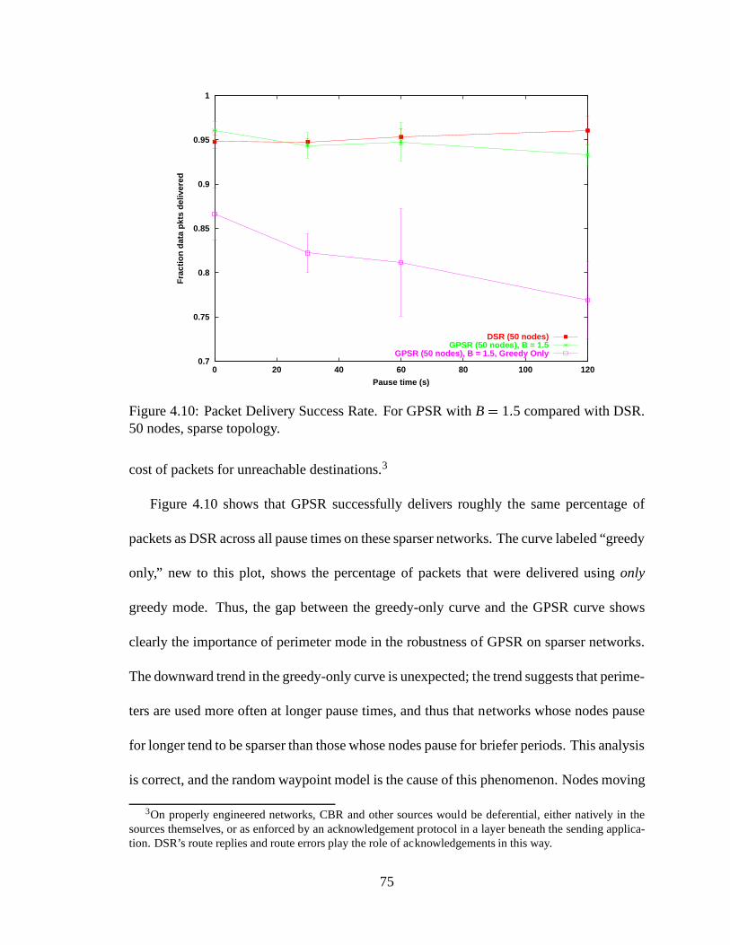
0.7
0.75
0.8
0.85
0.9
0.95
1
0 20 40 60 80 100 120
Fra
ctio
n d
ata
pkt
s d
eliv
ered
Pause time (s)
DSR (50 nodes)GPSR (50 nodes), B = 1.5
GPSR (50 nodes), B = 1.5, Greedy Only
Figure 4.10: Packet Delivery Success Rate. For GPSR withB= 1:5 compared with DSR.50 nodes, sparse topology.
cost of packets for unreachable destinations.3
Figure 4.10 shows that GPSR successfully delivers roughly the same percentage of
packets as DSR across all pause times on these sparser networks. The curve labeled “greedy
only,” new to this plot, shows the percentage of packets thatwere delivered usingonly
greedy mode. Thus, the gap between the greedy-only curve andthe GPSR curve shows
clearly the importance of perimeter mode in the robustness of GPSR on sparser networks.
The downward trend in the greedy-only curve is unexpected; the trend suggests that perime-
ters are used more often at longer pause times, and thus that networks whose nodes pause
for longer tend to be sparser than those whose nodes pause forbriefer periods. This analysis
is correct, and the random waypoint model is the cause of thisphenomenon. Nodes moving
3On properly engineered networks, CBR and other sources would be deferential, either natively in thesources themselves, or as enforced by an acknowledgement protocol in a layer beneath the sending applica-tion. DSR’s route replies and route errors play the role of acknowledgements in this way.
75

under the random waypoint model are in one of two states: moving, or paused. Because
destinations are chosen uniformly at random, a paused node is equally likely to be toward
the periphery of the simulated region or toward the center ofit. However, moving nodes
aremore likely to be toward the center of the region, because on average, a node moving
from one uniformly randomly selected position to another will tend to cross the center of
the region rather than remain in the outer periphery of the region. Thus, the greater the
fraction of nodes that are in the moving state, the more clustered the topology is toward the
center of the region, and the greater the fraction of nodes that are paused, the more rela-
tively dispersed the nodes are. We verified this effect empirically by measuring the number
of nodes in the circle of diameter 670 meters, centered in the1340-by-1340-meter region,
over time, for each pause time. This property of the random waypoint model may mirror
reality in some applications, in the sense that in a metropolitan area, mobile users may tend
to cross the center of the area during the work day, but be moredispersed on average while
stationary in the evening.
Figure 4.11 reveals that GPSR exhibits lower routing protocol overhead than DSR on
these sparser networks. The number of packets sent for disconnected destinations is re-
sponsible for DSR’s increased routing protocol overhead beyond that in the dense 50-node
simulations. Moreover, DSR’s caching is likely less effective in sparser topologies than in
denser ones, because nodes promiscuously overhear source routes less often.
Figure 4.12 shows the cost GPSR pays on sparse networks: non-shortest-path packet
delivery. In these simulations, GPSR delivers more packetsalong longer-than-optimal
routes than in the ones of denser networks. While GPSR still delivers more packets than
76
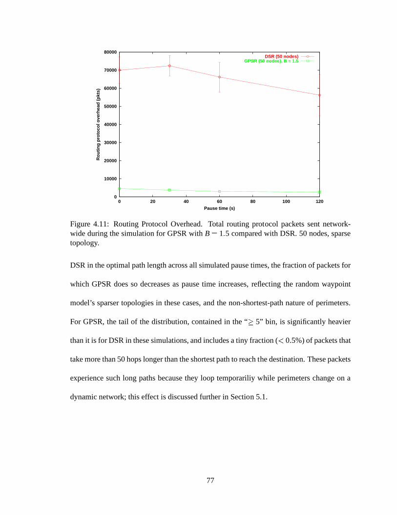
0
10000
20000
30000
40000
50000
60000
70000
80000
0 20 40 60 80 100 120
Ro
uti
ng
pro
toco
l ove
rhea
d (
pkt
s)
Pause time (s)
DSR (50 nodes)GPSR (50 nodes), B = 1.5
Figure 4.11: Routing Protocol Overhead. Total routing protocol packets sent network-wide during the simulation for GPSR withB= 1:5 compared with DSR. 50 nodes, sparsetopology.
DSR in the optimal path length across all simulated pause times, the fraction of packets for
which GPSR does so decreases as pause time increases, reflecting the random waypoint
model’s sparser topologies in these cases, and the non-shortest-path nature of perimeters.
For GPSR, the tail of the distribution, contained in the “� 5” bin, is significantly heavier
than it is for DSR in these simulations, and includes a tiny fraction (< 0.5%) of packets that
take more than 50 hops longer than the shortest path to reach the destination. These packets
experience such long paths because they loop temporariliy while perimeters change on a
dynamic network; this effect is discussed further in Section 5.1.
77
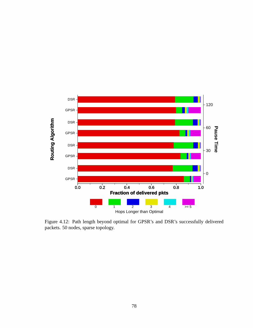
0.0 0.2 0.4 0.6 0.8 1.0Fraction of delivered pkts
GPSR
DSR
GPSR
DSR
GPSR
DSR
GPSR
DSR
0.0 0.2 0.4 0.6 0.8 1.0Fraction of delivered pkts
0
30
60
120
Pau
se Tim
e
0.0 0.2 0.4 0.6 0.8 1.0Fraction of delivered pkts
Ro
uti
ng
Alg
ori
thm
Hops Longer than Optimal
Ro
uti
ng
Alg
ori
thm
0 1 2 3 4 >= 5
Figure 4.12: Path length beyond optimal for GPSR’s and DSR’ssuccessfully deliveredpackets. 50 nodes, sparse topology.
78
4.7 State per Router
When measuring state per router, the relevant metric is the number ofnodesin a router’s
tables—not the number of routes. Because DSR uses source routes, each route stored by a
DSR router requires storage for each node along the route.
We measure both GPSR’s and DSR’s average per-node state for the set of 200-node
simulations with pause time 0. Because the state maintainedby a node in these networks
changes constantly, we take a snapshot at time 300.0 secondsin each of our 900-second
simulations, and measure the state in use by each node at thatinstant. A GPSR node
stores state for 26 nodes on average in the pause-time-0, 200-node simulations. This figure
depends on node density, as the only state a GPSR router keepsis an entry for each of its
single-hop radio neighbors. Note that as number of nodes andnetwork diameter increase
in the 50-, 112-, and 200-node simulations, GPSR stores the same quantity of state, as the
density of nodes remains fixed.
In comparison, the average DSR node in our 200-node, pause-time-0 simulation stores
state for 266 nodes—more than the total number of destinations in the network. It should
be noted that this value for DSR is clamped by the fixed-size route cache in the DSR
simulator’s implementation; this cache is limited to 64 routes. While DSR might profit
in robustness from a larger route cache, the state cost per node will increase dramatically
as the network size increases, and increasingly many more diverse routes are discovered.
A larger DSR route cache will also store more broken routes, as mobility and network
diameter increase. Figure 4.13 compares the state size stored on average by DSR and
GPSR, in both nodes and bytes.
79
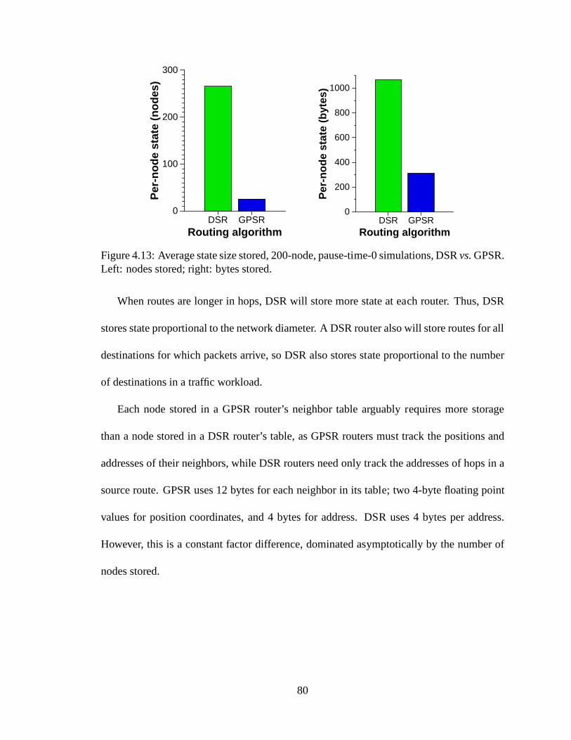
DSR GPSRRouting algorithm
0
100
200
300
Per
-no
de
stat
e (n
od
es)
DSR GPSRRouting algorithm
0
200
400
600
800
1000
Per
-no
de
stat
e (b
ytes
)
Figure 4.13: Average state size stored, 200-node, pause-time-0 simulations, DSRvs.GPSR.Left: nodes stored; right: bytes stored.
When routes are longer in hops, DSR will store more state at each router. Thus, DSR
stores state proportional to the network diameter. A DSR router also will store routes for all
destinations for which packets arrive, so DSR also stores state proportional to the number
of destinations in a traffic workload.
Each node stored in a GPSR router’s neighbor table arguably requires more storage
than a node stored in a DSR router’s table, as GPSR routers must track the positions and
addresses of their neighbors, while DSR routers need only track the addresses of hops in a
source route. GPSR uses 12 bytes for each neighbor in its table; two 4-byte floating point
values for position coordinates, and 4 bytes for address. DSR uses 4 bytes per address.
However, this is a constant factor difference, dominated asymptotically by the number of
nodes stored.
80
Chapter 5
Discussion and Future Work
In this chapter, we describe the characteristics of networks where we expect GPSR to work
best and worst; discuss system design choices for GPSR networks; and suggest future
directions for extending and enhancing GPSR.
5.1 GPSR’s Properties
The mobile simulation results presented in Chapter 4 show that GPSR remains robust on
networks of increasing diameter and node count, while continuing to exhibit small routing
protocol overhead. The simulated networks were all of equaldensity to those simulated by
Brochet al. in [7]. The density of these networks has an important implication for GPSR:
it means that greedy forwarding can be used for the vast majority of packet forwarding de-
cisions. This relationship between density and the successof greedy forwarding alone was
shown in Chapter 2. Greedy forwarding approximates shortest paths well on these dense
networks, and its use of only local topological informationallows it to recover quickly from
81
the loss of a neighbor, and benefit quickly from the acquisition of a neighbor.
On sparser networks, perimeter mode will be used more frequently. Packets that use
perimeter mode tend to be delivered in longer than the shortest-path number of hops for two
reasons. First, a packet may greedily traverse hops that take it on a “blind alley” toward the
destination, that must effectively be retraced in perimeter mode. Second, perimeter mode,
is by nature circuitous in the paths it traces around planar faces, which only use a subset of
the full radio graph’s edges.
In addition, perimeters are less robust than greedy forwarding under mobility. While
a packet tours the interior of a planar face, the topology canchange such that an inner
face, that shares its boundary with the outer face the packetwas touring, but is narrower in
diameter than the outer face, closes around the packet. Thisinner face may not cross the
line between the packet’s point of entry into perimeter modeand the packet’s destination.
If it does not, the packet will endlessly loop around the inner face, until the inner face
reopens or moves to cross the line to the destination, or until the packet is dropped when its
time-to-live maximum hop counter reaches zero. An example of this phenomenon appears
in Figure 5.1. Here,S sends a packet toD, and while the packet traverses the perimeter
of the large void by the right-hand rule, nodex moves such that the two dashed edges are
newly created. Because the new inner perimeter involvingx does not cross the line from the
point of entry into perimeter mode toD, the packet will loop on the inner perimeter until
its TTL is decremented to zero. Note that the first edge of the outer perimeter recorded in
the packet by GPSR is not useful in detecting this inner loop.
It is important to note that the described inner-face phenomenon occurs less frequently
82
x
S
D
Figure 5.1: An inner perimeter closing around a packet.
as density decreases; the closing of an inner face requires nodes to be placed to form an
entire face within the outer one. This relationship is virtuous, in that perimeters are used
for forwarding more often as density decreases. Perimeter mode is sufficiently robust on
sparse, mobile networks to contribute significantly to the percentage of packets delivered
successfully by GPSR, as shown in the sparse network resultsin the previous chapter.
Few routing protocols are loop-free on dynamic topologies.The small class that are
trade off routing protocol overhead for loop freedom—they send protocol messages in an
attempt to force consistency on the routes chosen at nodes. If the topology changes more
quickly than they respond, these protocols suffer unreachability of destinations. This phe-
nomenon is clearly demonstrated in [7]: the DSDV protocol uses sequence numbers to
force consistency on routes. When the protocol doesn’t aggressively push sequence num-
ber changes (caused by route changes) throughout the network, it fails to route to many
destinations. When it does push sequence number changes aggressively, it generates large
83
routing protocol overhead. DSR is immune to looping traffic,because it uses source routes,
which can be constructed so as not to contain cycles. However, it suffers similarly as DSDV
does under mobility: as shown in Chapter 4, DSR must generatelarge volumes of routing
protocol traffic to relearn working, loop-free routes on mobile networks of wide diameter.
The majority of routing protocols, which are non-loop-freeunder dynamic topologies,
exhibit transient looping behavior after topology changes. The inner face behavior is tran-
sient in this way: once the inner face forms, it only traps packets inside it, and subsequent
packets between the same source and destination pair will beforwarded without looping.
An adversary can always move nodes so as to provoke looping behavior by these protocols,
and can do so in GPSR by endlessly creating new inner faces.
Synthesizing the above, we take the view that perimeters area recovery mechanismfor
greedy forwarding. They allow greedy forwarding to reach 100% of connected destinations
on static networks, and improve the robustness of greedy forwarding on mobile networks,
as well. The classic challenges for routing protocols are routing on dynamic topologies,
topologies with numerous nodes, or topologies with both these characteristics. GPSR has
been shown to scale well on dense, large-scale mobile networks and on sparser mobile
networks. It also will scale well on relatively static topologies with large numbers of nodes
(e.g., rooftop networks [37]), where pushing global state, even infrequently, is prohibitively
expensive because of the number of destinations in the network.
We expect that for any fixed node density, as the diameter of the network increases,
there exists a threshold diameter beyond which GPSR will deliver a greater fraction of
packets successfully than DSR. The measurements in Section4.5 show this trend on dense
84
networks. On sparser networks, GPSR will use perimeters more frequently. Perimeter-
mode forwarding is less robust than greedy-mode forwardingunder mobility. Starting from
a 50-node sparse network of the type simulated in Section 4.6, let us build a wider-diameter
network of equal density, by tiling several such 50-node sparse networks adjacent to each
other, in ann-tile-by-n-tile grid. The average end-to-end route length in the wider-diameter
network increases withn. And the frequency with which a DSR source route breaks on
average will also increase withn. Thus, as network diameter increases, under mobility, the
routes learned by a source node under DSR will be valid for progressively shorter intervals,
and in the limit, a DSR source will not succeed in learning routes that are still valid by
the time they return, if they return at all. In contrast, GPSRdoes not use end-to-end state
in forwarding. Thus, the chance that GPSR succeeds in forwarding a packet at each hop,
whether in greedy mode or perimeter mode, depends only on thelocal topology, which
depends on the density of nodes and mobility rate, and not thenetwork diameter. On
average, GPSR should succeed in routing a packet across eachof the n2 tiles with equal
probability. This argument suggests that GPSR will offer lower delivery success rates as
network diameter increases, as is borne out in the results inChapter 4. In summary, each
GPSR forwarding decision uses only local state, whose accuracy isindependent of network
diameter, while DSR uses end-to-end state, whose accuracydepends on network diameter.
5.2 System Design for GPSR Networks
The addition of location registration and lookup traffic fora location database will increase
GPSR’s overhead. For bidirectional traffic flows between endnodes, a location database
85
lookup will often need only be performed by the connection initiator at the start of a con-
nection; thereafter, both connection endpoints keep one another apprised of their changing
locations by stamping their current locations in each data packet they transmit. In this case,
the actual location database lookup is a one-time, DNS-likelookup.
It is important to note that GPSR decouples participation inrouting as a forwarder from
participation in the location database. Only nodes that aretraffic destinations need send
location updates to the database, and only nodes that originate traffic need send location
queries to it. In a dense sensor network [19], it is easy to imagine configuring only a small
subset of sensor nodes to take measurements at only the current points of interest, by flood-
ing a few configuration packets through the network. The remainder of the sensor network
can provide a robust transit network for the collection of measurements from sensors to the
measurement point, with GPSR’s beacons as their only routing protocol traffic—without
generating any traffic to and from the location database.
In some networks, a destination may inherently have a well-known location. For exam-
ple, the position of one or more fixed data collection points for a sensor network may be
known to all sensors, in which case no location database is needed.
It is also important to note that queries and registrations for the location database are
routable using GPSR itself; the queries and registrations are geographically addressed.
GRID [25] is an instance of just such a location database system, whose packets are all
generated with native geographical addresses.
Storing nodes’ velocity vector information in the locationdatabase, besides their in-
stantaneous positions, would allow extrapolation of nodes’ positions without additional
86
queries to the location database. This technique is promising because the predictability of
an object’s motion tends to be correlated with the object’s velocity (e.g.,passenger jets, au-
tomobiles on Interstate highways), though there are of course exceptions, such as military
fighter jets.
5.3 Future Work
One assumption in the use of planar perimeters we would like to investigate further is that a
node can reach all other nodes within its radio range. The GG and RNG planarizations both
rely on a node’s ability to accurately know if there is a witnessw within radio range, when
considering elimination of an edge to a known neighbor. Our use of the GG and RNG can
disconnect a graph with particular patterns of obstacles between nodes. This disconnection
is easily avoided by forcing the pair of nodes bordering an edge to agree on the edge’s fate,
with two rules:� Both nodes must decide to eliminate the edge, or neither willdo so.� If both nodes decide to eliminate the edge, they must agree ona commonw (i.e.,
there must be a transitive path through a witness they canbothreach).
However, this modification to the planarization algorithmswill make the RNG and GG
planarizations leave one or more crossing edges in these regions with obstacles. We intend
to study these cases further. One promising approach in dealing with such obstacles may
be to have obstructed nodes choose a reachablepartner node elsewhere in the network,
and route via the partner for destinations that are unreachable because of local failure of
87

the planarization. One engineering choice that can assist in avoiding difficulties caused
by barriers to radio propagation is to choose a conservativethreshold distance for the ra-
dios, and to ignore links to neighbors who are reachable but located beyond this threshold.
Such a choice allows one to deploy nodes more densely to engineer away barriers to radio
propagation. For example, 900 MHz battery-powered radios,such as Metricom Ricochet
radios, which transmit at 1 W, propagate their signal so wellindoors that a single radio on
the top floor of a large building can reach other radios at any point in the building. Thus,
it is possible to build radios where barriers such as multiple walls and floors still allow a
reasonable conservative threshold distance under which connectivity is assured.
Hybridizing GPSR with Distance-Vector routing may both improve GPSR’s robustness
in the presence of obstacles, and allow GPSR to recover from imprecision in the destination
location stamped in a packet, caused by the continuing motion of the destination between
the time it reported its location to the location database and when a packet is forwarded
using that imprecise location. First, we note that the beaconing protocol conducted by
GPSRis a kind of Distance-Vector routing, where the propagation ofnodes’ information is
limited to a single hop. Ak-hop Distance-Vector protocol propagates nodes’ positionand
transitive reachability information fork hops. Increasingk in GPSR’s beaconing protocol
would provide information to nodes about the entire set of reachable destinations within
k hops of them. Obstacles are most often local phenomena. Localized shortest-path (k-
hop DV) routing would assist nodes in forwarding around local obstacleswithout using
perimeters. Moreover, a packet only needs to reach a node withink hops of the destination’s
current position to be forwarded successfully to the destination. So increasingk would
88
increase GPSR’s tolerance for imprecision in packets’ destination location fields. Of course
increasingk will increase GPSR’s routing protocol overhead, both because the number of
nodes mentioned in a beacon packet will increase, and because more frequent beacons will
be necessary to keep consistent topological state at all nodes.
While we have shown herein the benefits of geography as a tool for scalable routing
systems, measuring the combined behavior of GPSR and a location database system will
reveal more about the costs of using geography for routing. An efficient distributed location
database would provide a network service useful in many other location-aware computing
applications.
A comparison of the behavior of GPSR using the RNG and GG planarizations would
reveal the performance effects of the tradeoff between the greater traffic concentration that
occurs in perimeter forwarding on the sparser RNG,vs.the increased spatial diversity that
the RNG offers by virtue of its sparsity. Even outside the context of GPSR, it may be the
case that limiting edges used for forwarding in a radio network to those on the RNG or GG
may reduce contention and improve efficiency on MAC protocols sensitive to the number
of sending stations in mutual range.
Provisioning of bandwidth for geographically routed networks is an open problem. On
wired networks, low capacity links exist at the edges of the network, which aggregate into
higher capacity links, and so on; capacity is provisioned hierarchically, and hierarchical
routing (BGP over an intra-domain routing protocol) matches the hierarchical capacity. On
a naive rooftop network in a metropolitan area, where all radios have equal capacity, “hot
spots” of traffic concentration can cause congestion. Thesehot spots will occur when con-
89
nections are geographically routed through the same region. We believe that geographic
routing is naturally suited to a new kind of traffic provisioning that is not hierarchical, but
geographic. Specifically, at flow setup time between a sourceand destination, a random
geographic waypoint (or set of waypoints) can be chosen, andthe flow forced to traverse
those waypoint(s). The effect of such a scheme would be to spread the traffic spatially
across the network. Routes would become non-shortest-path, but that effect exists in to-
day’s hierarchically provisioned networks. In fact, the operational definition of provision-
ing is elevation of capacity’s importance above hop count’sin making routing decisions.
The fundamental reason that this scheme can work is that on a wireless network,capacity
is correlated with geography, since spatial diversity increases capacity.
Hierarchy, useful in improving the scalability of wired Internet routing systems, should
enhance GPSR’s scalability as well, in networks where thereare static boundaries for rout-
ing sub-domains. In networks whose nodes have heterogeneous radio ranges, and which
are therefore not unit graphs, GPSR may not be able to make useof the longest links. A
campus comprised of intra-campus links up to 250 m in length may have a 2 km point-
to-point link to another site that terminates in the center of the local campus. If the entire
network is a single geographic routing domain, nodes located between the center of the
local campus and the remote site will forward greedily toward the boundary of the local
campus, and the path to the remote site from this boundary will not consist of faces that are
progressively closer to the destination, as is the case in networks that are unit graphs. Hi-
erarchy can salvage this situation: nodes inside the local campus can geographically route
packets destined for outside the campus to position of the campus gateway. Intra-campus
90
links comprise a unit graph with one threshold, and inter-campus links comprise a separate
unit graph, the upper level in the hierarchy, with a greater threshold. Finn [10] touches on
the potential utility of hierarchy in greedy geographic routing.
We hope to extend GPSR for hosts placed in three-dimensionalspace, beyond the flat
topologies explored in this thesis. Greedy forwarding extends simply to three dimensions.
However, a three-dimensional analog for planar perimeter forwarding is harder to achieve.
A promising approach is to implement perimeter forwarding for 3-D volumesrather than
2-D faces. There exists an algorithm for computing the Relative Neighborhood Graph for
a set of points placed in three dimensions [40] (the result isa graph in which no plane
cutting the 3-D space contains two crossing edges—a lattice-like structure). However, this
algorithm is not distributed in the way the two-dimensionalone is; it requires the entire
topology be known to a single entity computing the RNG. Traversing the surfaces of these
volumes will be more akin to search than to the straightforward, cycle-traversing right-hand
rule.
91
Chapter 6
Related Work
Finn [10] is the earliest we know to propose greedy routing using the locations of nodes. He
recognizes the small forwarding state greedy forwarding requires, and observes the failure
of greedy forwarding upon reaching a local maximum. He proposes flooding search for a
closer node as a strategy for recovering from local maxima.
We first propose greedy forwarding and perimeter traversal in [22], as briefly discussed
in Section 3.1. This work simulates this older algorithm on static networks, in a very
idealized (contentionless, infinite bandwidth) simulator, and presents the state per node
(including perimeter node lists, notably absent from the current work), message cost from
cold start to convergence, and frequency with which routes are not found, because of the
imperfect no-crossing heuristic. This prior work does not offer any mobile simulation re-
sults, and the earlier algorithm suffers in many ways from its maintenance of state beyond
neighbor lists at all routers: increased state size for perimeter lists at all nodes, periodic
pro-active routing protocol traffic that perimeter probes generate, and staleness of perime-
92
ter lists that would occur under mobility. The unreachability of even a small fraction of
destinations onstatic networks because of the failure of the no-crossing heuristic is also
problematic; such routing failures are permanent, not transitory.
Johnson and Maltz [18] propose the Dynamic Source Routing (DSR) protocol. DSR
generates routing traffic reactively: a router floods a routerequest packet throughout the
network. When the request reaches the destination, the destination returns a route reply
to the request’s originator. Nodes aggressively cache routes that they learn, so that inter-
mediate nodes between a querier and destination may subsequently reply on behalf of the
destination, and limit the propagation of requests. More recently, Hu and Johnson [16]
evaluate a variety of caching schemes for DSR under several mobility models, and present
measurements of their relative performance taken on 50-node networks.
Brochet al. [7] compare the performance of the DSDV, TORA, DSR, and AODV rout-
ing protocols on a simulated mobile IEEE 802.11 network. They simulate networks of
50 nodes, under a range of mobility rates and traffic loads. Their measurements show the
effectiveness of DSR’s caching in minimizing DSR’s routingprotocol traffic on these 50-
node networks. DSR and AODV deliver by far more packets successfully with by far less
routing protocol overhead than the other algorithms measured when mobility is most rapid.
In the interest of comparability of results, we use this work’s ns simulation environment for
IEEE 802.11, a two-ray ground reflection model, and DSR.
Ko and Vaidya [24] describe Location Aided Routing (LAR), anoptimization to DSR
in which nodes limit the propagation of route request packets to the geographic region
where it is most probable the destination is located. LAR uses base DSR to establish first
93
connectivity with a destination; thereafter, a route querier learns the destination’s location
directly from the destination node, and uses this information to mark route requests for
propagation only within a region of some size about the destination’s last known posi-
tion. Like DSR’s caching, LAR is a strategy for limiting the propagation of route requests.
When a circuitous path, outside the region LAR limits route request propagation within,
becomes the only path to a destination, LAR reverts to DSR’s flooding-with-caching base
case. Under LAR, DSR’s routes are still end-to-end source routes. Geography is not used
for data packet forwarding decisions under LAR; only to scope routing protocol packet
propagation.
Basagniet al.[2] present DREAM, an integrated location dissemination and geographic
routing system. In DREAM, all nodes store a location table mapping every node’s address
to its position. Every node originates position reports periodically, at a rate proportional
to its own mobility rate. Position reports are flooded, but they are propagated varying
distances. Nodes originate position reports most frequently with short distance propagation
limits, and most rarely with long (i.e., network-wide) propagation limits. In this regime, the
precision of a location table entry for a destination is greatest in nodes near that destination,
and progressively less in nodes increasingly farther away.This strategy avoids flooding
position reports network-wide as frequently as a naive flooding protocol, and exploits the
fact that the direction of the destination is less sensitiveto error in the destination’s position,
the farther one is from the destination. Packets are marked only with the destination’s
address. To forward a packet, a node looks up the location of the destination in its local
location table, and forwards the packet to all its neighborsin the direction of the destination,
94
where “in the direction of” is defined as within an arc centered on the destination. DREAM
uses the estimated movement rate of the destination to boundthe destination’s position
within a circular region. The arc inside which the packet is forwarded is bounded by the two
lines from the forwarding node that are tangent to this circle about the destination. When
the forwarding node has no neighbors within this arc, it drops the packet. DREAM forces
all packets to be sent reliably by their originator, and the originator falls back on flooding
(or other techniques, unspecified by Basagniet al.) to discover a route to the destination
when no acknowledgement returns for a packet. DREAM can deliver exponentially many
copies of a packet to the destination; at each hop, the packetis forwarded toall neighbors
within the arc in the appropriate direction, and those duplicates are in turn duplicated at
subsequent hops. The authors argue that this packet duplication is a robustness feature, but
it is unnecessarily wasteful of the network’s capacity. Linand Stojmenovic [26] present an
example in which DREAM will loop traffic, even on astaticnetwork, assuming a relatively
large forwarding arc. However, because the choice of arc when the destination has afixed
position is not explained in [2], this example may or may not be relevant.1
Li et al. [25] propose GLS, a scalable and robust location database that geographically
addresses queries and registrations. Their system dynamically selects multiple database
servers to store each node’s location, for robustness against server failure. This property
also ensures that a cluster of nodes partitioned from the remainder of the network con-
tinues to have location database service, provided by nodesinside the cluster. GLS uses a
geographic hierarchy to serve queries at a server topologically close to the querier. The sys-
1As specified in [2], one would expect the arc to be zero degreeswhen the position of the destination isfixed. But this would mean the forwarder would forward only tonodes exactlyon the line to the destination.
95

tem spreads the work of the location database evenly across all nodes, by usingConsistent
Hashing[20] to induce separate caching hierarchies for each node’sposition information.
Boseet al. [5] independently investigated the graph algorithms for rendering a radio
network’s graph planar. They suggest the Gabriel Graph, andanalyze the increase in path
length over shortest paths when traversing a graph usingonlyperimeters. Motivated by the
longer-than-optimal paths perimeter traversal alone finds, they suggest combining planar
graph traversal with greedy forwarding, and verify that this combination produces path
lengths closer to true shortest paths. They present these algorithms at an abstract level.
They do not present a routing protocol, do not simulate a network at the packet level, and
assume that all nodes are stationary and reachable. In a revised version of this work [6],
Boseet al. state that the extension of their static graph traversal algorithms to dynamic,
changing networks is an open problem, and that they are unsure of how to evaluate the
mobile versions of their algorithms in simulation.
96
Chapter 7
Conclusion
We have presented Greedy Perimeter Stateless Routing, GPSR, a routing algorithm that
uses geography to achieve small per-node routing state, small routing protocol message
complexity, and extremely robust packet delivery on densely deployed wireless networks.
GPSR forwards greedily where topology allows, and benefits from the robustness and ten-
dency toward shortest paths of greedy forwarding. Where greedy forwarding is impossi-
ble, GPSR uses perimeter forwarding to recover, and reach a region of the network where
greedy forwarding can resume. Perimeter forwarding diverges from shortest paths, and is
sometimes transitorily less robust for packets in mid-traversal on a perimeter that changes.
GPSR scales well as the number of nodes and mobility rate increase. Our simulations on
dense mobile networks with up to 200 nodes over a full IEEE 802.11 MAC demonstrate
GPSR’s scalability: GPSR consistently delivers upwards of94% of data packets success-
fully; it is competitive with DSR in this respect on 50-node networks at all pause times,
and increasingly more successful than DSR as the number of nodes increases, as demon-
97
strated on 112-node and 200-node networks. GPSR generates routing protocol traffic in a
quantity independent of the length of the routes through thenetwork, and therefore gener-
ates a constant, low volume of routing protocol messages as mobility increases, yet doesn’t
suffer from decreased robustness in finding routes. DSR mustquery longer routes as the
network diameter increases, and must do so more often as mobility increases, and caching
becomes less effective. Thus, DSR generates drastically more routing protocol traffic in our
200-node and 112-node simulations than it does in our 50-node ones. Finally, GPSR keeps
state proportional to the number of its neighbors, while both traffic sources and intermedi-
ate DSR routers cache state proportional to the product of the number of routes learned and
route length in hops.
We note that DSR by design does not make use of geographic information. This point,
while far from subtle, is worth mentioning explicitly because GPSR benefits greatly from
using information beyond that available to DSR.
In this thesis, we contribute:� An architectural description of geographic forwarding as ascaling strategy for rout-
ing, and its relationship to hierarchy and caching, two other routing scaling strategies.� A description of application areas where routing faces scaling challenges in number
of nodes and rate of motion of nodes.� The application of planar graphs to routing for wireless networks, to allow recovery
from greedy forwarding failure on all static networks.� The GPSR routing algorithm, which performs all forwarding decisions at a node
98
usingonly information concerning that node’s immediate, single-hopneighbors.� The full, dynamic GPSR routing protocol, designed for robustness on mobile net-
works, including integration with feedback from the MAC layer, dynamic triggering
of the planarization algorithm, and support for detecting and dropping packets for
disconnected destinations.� A detailed, simulation-based performance evaluation of the GPSR and DSR mobile
routing protocols on mobile networks, that shows GPSR scales well in increasing
number of nodes and mobility by keeping small state, and shows that DSR-style
source routing with caching does not scale, because caching’s effectiveness declines
with mobility and network diameter.
GPSR’s benefits all stem from geographic routing’s use of only immediate-neighbor in-
formation in forwarding decisions. Routing protocols thatrely on end-to-end state concern-
ing the path between a forwarding router and a packet’s destination, as do source-routed,
DV, and LS algorithms, face a scaling challenge as network diameter in hops and mobil-
ity increase because the product of these two factors determines the rate that end-to-end
paths change. Hierarchy and caching have proven successfulin scaling these algorithms.
Geography, as exemplified in GPSR, represents another powerful lever for scaling routing.
99
Bibliography
[1] A BRAMSON, N. The ALOHA system - another alternative for computer communi-
cations.AFIPS 37(1970), 281–285.
[2] BASAGNI, S., CHLAMTAC , I., SYROTIUK, V., AND WOODWARD, B. A distance
routing effect algorithm for mobility (DREAM). InProceedings of the Fourth Annual
ACM/IEEE International Conference on Mobile Computing andNetworking (Mobi-
Com ’98)(Dallas, Texas, USA, Aug. 1998), pp. 76–84.
[3] BETTENDORFF, J. Personal communication. Metricom, Inc., Sept. 1997.
[4] BHARGHAVAN , A., DEMERS, S., SHENKER, S., AND ZHANG, L. MACAW: A
media access protocol for wireless LANs. InProceedings of the SIGCOMM ’94
Conference on Communications, Architectures, Protocols,and Applications(Sept.
1994), pp. 212–225.
[5] BOSE, P., MORIN, P., STOJMENOVIC, I., AND URRUTIA, J. Routing with guar-
anteed delivery inad hocwireless networks. Workshop on Discrete Algorithms and
Methods for Mobile Computing and Communications (DialM ’99), Aug. 1999.
100
[6] BOSE, P., MORIN, P., STOJMENOVIC, I., AND URRUTIA, J.
Routing with guaranteed delivery in ad hoc wireless networks.
http://www.site.uottawa.ca/ ivan/unitgraphs.ps, Dec. 1999.
[7] BROCH, J., MALTZ , D., JOHNSON, D., HU, Y., , AND JETCHEVA, J. A performance
comparison of multi-hop wireless ad hoc network routing protocols. InProceedings
of the Fourth Annual ACM/IEEE International Conference on Mobile Computing and
Networking (MobiCom ’98)(Dallas, Texas, USA, Aug. 1998).
[8] CALI , F., CONTI, M., AND GREGORI, E. IEEE 802.11 wireless LAN: capacity
analysis and protocol enhancement. InProceedings of IEEE INFOCOM 1998(San
Francisco, California, March/April 1998), p. 142.
[9] CHANDRAKASAN , A., AMIRTHARAJAH, R., CHO, S., GOODMAN, J., KONDURI,
G., KULIK , J., RABINER, W., AND WANG, A. Design considerations for distributed
microsensor systems. InProceedings of the IEEE 1999 Custom Integrated Circuits
Conference (CICC ’99)(May 1999), pp. 279–286.
[10] FINN , G. G. Routing and addressing problems in large metropolitan-scale internet-
works. Tech. Rep. ISI/RR-87-180, Information Sciences Institute, Mar. 1987.
[11] FLOYD , S.,AND JACOBOSON, V. The synchronization of periodic routing messages.
IEEE/ACM Transactions on Networking 2, 2 (April 1994), 122–136.
[12] GABRIEL, K., AND SOKAL , R. A new statistical approach to geographic variation
analysis.Systematic Zoology 18(1969), 259–278.
101

[13] HAAS, Z., AND PEARLMAN , M. The performance of query control schemes for the
zone routing protocol. InProceedings of the SIGCOMM ’98 Conference on Commu-
nications Architectures, Protocols and Applications(Sept. 1998).
[14] HEDRICK, C. E. Routing information protocol. Internet Request for Comments RFC
1058, June 1988.
[15] HOU, T., AND L I , V. Performance analysis of routing strategies in multihoppacket
radio networks. InProceedings of IEEE GLOBECOM 1984(1984), pp. 487–492.
[16] HU, Y., AND JOHNSON, D. Caching strategies in on-demand routing protocols for
wireless ad hoc networks. InProceedings of the Sixth Annual ACM/IEEE Interna-
tional Conference on Mobile Computing and Networking (MobiCom 2000)(Boston,
Massachusetts, USA, Aug. 2000).
[17] IEEE COMPUTER SOCIETY LAN MAN S TANDARDS COMMITTEE. Wireless LAN
Medium Access Control (MAC) and Physical Layer (PHY) Specifications. IEEE
Std. 802.11-1997, 1997.
[18] JOHNSON, D. B., AND MALTZ , D. B. Dynamic source routing in ad hoc wireless
networks. InMobile Computing, T. Imielinski and H. Korth, Eds. Kluwer Academic
Publishers, 1996, ch. 5, pp. 153–181.
[19] KAHN, J. M., KATZ , R. H., AND PISTER, K. S. J. Mobile networking for smart
dust. InProceedings of the Fifth Annual ACM/IEEE International Conference on
Mobile Computing and Networking (MobiCom ’99)(Seattle, WA, USA, Aug. 1999).
102
[20] KARGER, D., LEHMAN, E., LEIGHTON, T., LEVINE, M., LEWIN, D., AND PANI -
GRAHY, R. Consistent hashing and random trees: Distributed caching protocols for
relieving hot spots on the world wide web. InProceedings of the 29th ACM Sympo-
sium on Theory of Computing(May 1997), pp. 654–663.
[21] KARN, P. MACA—a new channel access method for packet radio. InProceedings
of the 9th Computer Networking Conference(Sept. 1990), pp. 134–140.
[22] KARP, B. Greedy perimeter state routing. Invited Seminar at the USC/Information
Sciences Institute, July 1998.
[23] KARP, B., AND KUNG, H. GPSR: greedy perimeter stateless routing for wireless
networks. InProceedings of the Sixth Annual ACM/IEEE International Conference on
Mobile Computing and Networking (MobiCom 2000)(Boston, Massachusetts, USA,
Aug. 2000).
[24] KO, Y., AND VAIDYA , N. Location-aided routing in mobile ad hoc networks. In
Proceedings of the Fourth Annual ACM/IEEE International Conference on Mobile
Computing and Networking (MobiCom ’98)(Dallas, Texas, USA, Aug. 1998).
[25] L I , J., JANNOTTI , J., DECOUTO, D., KARGER, D., AND MORRIS, R. A scalable
location service for geographic ad-hoc routing. InProceedings of the Sixth Annual
ACM/IEEE International Conference on Mobile Computing andNetworking (Mobi-
Com 2000)(Boston, MA, USA, Aug. 2000).
[26] L IN , X., AND STOJMENOVIC, I. Gps-based routing algorithms for wireless net-
works. Tech. Rep. TR-98-10, SITE, University of Ottawa, Dec. 1998.
103
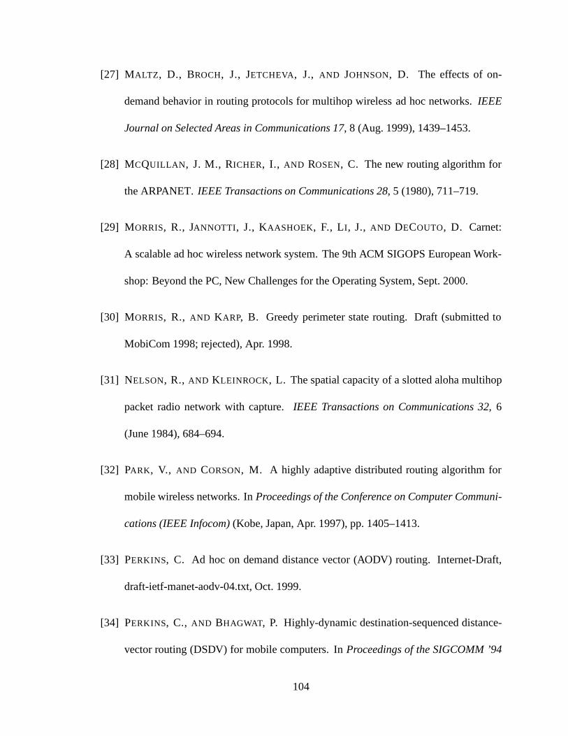
[27] MALTZ , D., BROCH, J., JETCHEVA, J., AND JOHNSON, D. The effects of on-
demand behavior in routing protocols for multihop wirelessad hoc networks.IEEE
Journal on Selected Areas in Communications 17, 8 (Aug. 1999), 1439–1453.
[28] MCQUILLAN , J. M., RICHER, I., AND ROSEN, C. The new routing algorithm for
the ARPANET.IEEE Transactions on Communications 28, 5 (1980), 711–719.
[29] MORRIS, R., JANNOTTI , J., KAASHOEK, F., LI , J., AND DECOUTO, D. Carnet:
A scalable ad hoc wireless network system. The 9th ACM SIGOPSEuropean Work-
shop: Beyond the PC, New Challenges for the Operating System, Sept. 2000.
[30] MORRIS, R., AND KARP, B. Greedy perimeter state routing. Draft (submitted to
MobiCom 1998; rejected), Apr. 1998.
[31] NELSON, R., AND KLEINROCK, L. The spatial capacity of a slotted aloha multihop
packet radio network with capture.IEEE Transactions on Communications 32, 6
(June 1984), 684–694.
[32] PARK , V., AND CORSON, M. A highly adaptive distributed routing algorithm for
mobile wireless networks. InProceedings of the Conference on Computer Communi-
cations (IEEE Infocom)(Kobe, Japan, Apr. 1997), pp. 1405–1413.
[33] PERKINS, C. Ad hoc on demand distance vector (AODV) routing. Internet-Draft,
draft-ietf-manet-aodv-04.txt, Oct. 1999.
[34] PERKINS, C., AND BHAGWAT, P. Highly-dynamic destination-sequenced distance-
vector routing (DSDV) for mobile computers. InProceedings of the SIGCOMM ’94
104
Conference on Communications, Architectures, Protocols,and Applications(London,
UK, Sept. 1994), pp. 234–244.
[35] PRIYANTHA , N., CHAKRABORTY, A., AND BALAKRISHNAN , H. The cricket
location-support system. InProceedings of the Sixth Annual ACM/IEEE Interna-
tional Conference on Mobile Computing and Networking (MobiCom 2000)(Boston,
Massachusetts, USA, Aug. 2000).
[36] SALTZER, J., REED, D. P.,AND CLARK , D. End-to-end arguments in system design.
ACM Transactions on Computer Systems 2, 4 (Nov. 1984), 277–288.
[37] SHEPARD, T. A channel access scheme for large dense packet radio networks. In
Proceedings of the SIGCOMM ’96 Conference on Communications Architectures,
Protocols and Applications(Aug. 1996).
[38] THE CMU MONARCH GROUP. Wireless and Mobility Extensions to ns-2.
http://www.monarch.cs.cmu.edu/cmu-ns.html, Oct. 1999.
[39] THE VINT PROJECT. The UCB/LBNL/VINT Network Simulator—ns (version 2).
http://mash.cs.berkeley.edu/ns.
[40] TOUSSAINT, G. The relative neighborhood graph of a finite planar set,.Pattern
Recognition 12, 4 (1980), 261–268.
[41] WARD, A., JONES, A., AND HOPPER, A. A new location technique for the active
office. IEEE Personal Communications 4, 5 (Oct. 1997), 42–47.
105
[42] ZAUMEN , W., AND GARCIA-LUNA ACEVES, J. Dynamics of distributed shortest-
path routing algorithms. InProceedings of the SIGCOMM ’91 Conference on Com-
munications Architectures, Protocols and Applications(Sept. 1991), pp. 31–42.
106